Munich Personal RePEc Archive

Estimating Difference-in-Differences in

the Presence of Spillovers

Clarke, Damian

Universidad de Santiago de Chile

September 2017

Online at https://mpra.ub.uni-muenchen.de/81604/

MPRA Paper No. 81604, posted 27 Sep 2017 05:06 UTC

Estimating Difference-in-Differences in the Presence ofSpillovers∗

Damian Clarke

September 14, 2017

Abstract

I propose a method for difference-in-differences (DD) estimation in situations where the stable

unit treatment value assumption is violated locally. �is is relevant for a wide variety of cases where

spillovers may occur between quasi-treatment and quasi-control areas in a (natural) experiment. A

flexible methodology is described to test for such spillovers, and to consistently estimate treatment

effects in their presence. �is spillover-robust DD method results in two classes of estimands: treat-

ment effects, and “close” to treatment effects. �e methodology outlined describes a versatile and

non-arbitrary procedure to determine the distance over which treatments propagate, where distance

can be defined in many ways, including as a multi-dimensional measure. �is methodology is illus-

trated by simulation, and by its application to estimates of the impact of state-level text-messaging

bans on fatal vehicle accidents. Extending existing DD estimates, I document that reforms travel

over roads, and have spillover effects in neighbouring non-affected counties. Text messaging laws

appear to continue to alter driving behaviour as much as 30 km outside of affected jurisdictions.

JEL codes: C13, C21, D04, R23, K42.

Keywords: Policy evaluation, difference-in-differences, spillovers, natural experiments, SUTVA

∗I thank Serafima Chirkova, Paul Devereux, James Fenske, Rossa O’Keeffe-O’Donovan, Rudi Rocha, Chris Roth andMar-garet Stevens for comments and suggestions which have improved this paper. I am also grateful to audiences at PUC Chile,Universidad de la Republica Uruguay, and participants in the Impact Evaluation Meeting at the Inter-American Develop-ment Bank for their comments. I gratefully acknowledge the financial support of FONDECYT (grant number 11160200)of the Government of Chile. Any remaining errors are my own. Full source code, including programs to implement theestimator in Stata, Matlab and R are available for download and use at h�ps://github.com/damiancclarke/cdifdif. Affiliation:Department of Economics, Universidad de Santiago de Chile. Contact email: damian.clarke@usach.cl.

1

1 Introduction

Natural experiments o�en rely on territorial borders to estimate treatment effects. �ese borders sepa-

rate quasi-treatment from quasi-control groups with individuals in one area having access to a program

or treatment while those in another do not. In cases such as these where geographic location is used

to motivate identification, the stable unit treatment value assumption (SUTVA) is, either explicitly or

implicitly, invoked.1

However, o�en territorial borders are porous. Generally state, regional, municipal, and village

boundaries can be easily, if not costlessly, crossed. Given this, researchers interested in using natu-

ral experiments in this way may be concerned that the effects of a program in a treatment cluster may

spillover into non-treatment clusters—at least locally.

Such a situation is in clear violation of the SUTVA’s requirement that the treatment status of any

one unit must not affect the outcomes of any other unit. In this paper I propose a methodology to deal

with such spillover effects. I discuss how to test for local spillovers, and if such spillovers exist, how

to estimate unbiased treatment effects in their presence. It is shown that this estimation requires a

weaker condition than SUTVA: namely that SUTVA holds between some units, as determined by their

distance from the treatment cluster. I discuss how to estimate treatment and spillover effects, and then

propose a method to generalise the proposed estimator to a higher dimensional case where spillovers

may depend in a flexible way on an arbitrary number of factors.

I show that this methodology recovers unbiased treatment estimates under quite general violations

of SUTVA. While it is assumed that the distance of an individual to the nearest treatment cluster deter-

mineswhether stable unit treatment type assumptions hold for that individual, ‘distance’ is defined very

broadly. It is envisioned that this will allow for phenomena such as information flowing from treated

to untreated areas, or of untreated individuals violating their treatment status by travelling from un-

treated to treated areas. In each case distance plays a clear role in the propagation of treatment; either

information must travel out, or beneficiaries must travel in. Similarly, this framework allows for local

general equilibrium-type spillovers, where a tightly applied program may have an economic effect on

nearby markets, but where this effect dissipates as distance to treatment increases.

�ismethodology has two particular features that make it suitable for application to empirical work.

Firstly, it places no strict restriction on the way in which spillovers propagate between individual ob-

servations and between treatment clusters. A range of other methods of estimating indirect policy

1�e SUTVA has a long and interesting history, under various guises. Cox (1958) refers to “no interference betweendifferent units”, before Rubin (1978) introduced the concept of SUTVA (the name SUTVA did not appear until Rubin (1980)).Recent work of Manski (2013), refers to this assumption as Individualistic Treatment Response (ITR). I provide additionaldiscussion of related literature in Appendix A of this paper.

2

effects have been proposed which are based on a hierarchical treatment assignment, where treatment

receipt is allowed to occur within a particular geographic cluster, but not to neighbouring clusters (see

for example Hudgens and Halloran (2008); Liu and Hudgens (2014); Baird et al. (forthcoming) for some

such cases). However, the spillover-robust difference-in-differences (DD) method laid out here allows

spillovers of treatments from treated clusters to non-treated clusters, with the only restriction being a

quite flexible geographical dependence of propagation. Secondly, the area over which spillovers occur

is determined in an optimising (non ad-hoc) way. A cross-validation method is proposed to determine

the size of distance bins to be considered, with some similarities to bandwidth search in regression dis-

continuity models. �is optimising procedure provides a simple automated rule to determine spillover

distances, which removes any parameter choices from a researcher’s control, allowing for the avoidance

of concerns that parameters may have been chosen in order to support a particular hypothesis. �is

procedure allows for spillovers to be determined endogenously from data. A data-snooping procedure

is illustrated, alongwith refinements for use with large datasets. �is described procedure is well-suited

to difference-in-difference applications which previously have based the estimation of externalities or

geographic spillovers on researcher-defined distance cut-offs (a number of important empirical exam-

ples of this type include Miguel and Kremer (2004) and Almond et al. (2009)).

In this paper, I first derive a simple closed form solution for the bias in DD models where spillovers

are present. I show that the bias in naive DD models depends only on (a) the magnitude and direction

of spillover effects on untreated observations, and (b) the proportion of the population impacted by

spillovers. A generalised bias formula is proven, allowing for the exact derivation of biases even in

cases where an arbitrary number of included and excluded treatment and “close to treatment” groups

are present in a regression model. �e performance of the proposed estimator is then examined, firstly,

by simulation, and secondly by application to a particular empirical example. Under simulation I show

that the proposed estimator recovers estimates of the treatment effect of interest, and has good size

properties, even in cases where spillovers occur to a large proportion of control units. �e estimator

is documented to perform well, even under model mis-specification of the precise nature of spillovers,

given the flexible modeling procedure employed.

In turning to empirics, thismethodology is illustrated by considering the case of the passage of state-

level text messaging bans for vehicle operators in the US. I return to the data and specifications of Abouk

and Adams (2013), who document the impacts of these text-messaging bans on fatal vehicle accidents

using single-vehicle single-occupant accidents, due to the increased likelihood that these accidents owe

to the use of mobile telephones. I revisit their estimates using the precise geographic location of each

accident, and county-level mortality figures for the US. Following their specifications and augmenting

with the spillover-robust DD method proposed here, I find that allowing for spillovers suggests that

counties which were not directly treated by the reform but which are located close to treated areas

3

are impacted in a similar way as those which were directly treated. �is is a relevant result for policy

evaluation, as it suggests that the reforms may have wider impacts than originally determined, and,

importantly, that drivers did not simply delay the sending of text messages until they were travelling

on roads in nearby areas without text messaging bans. �e optimal spillover procedure finds, however,

that changes in driver behaviour are perceptible over relatively short distances, of anywhere from 0-30

kilometres, depending on the reform type examined.

Although the empirical example uses a geographic measure of distance, this methodology should

not be considered as limited to only spatial spillovers. Univariate measures of distance including propa-

gation through nodes in a network, ethnic distance, ideological distance, or other quantifiable measures

of difference between units can be used in precisely the same manner with the results and techniques

described in this paper. I also show how multivariate measures of distance, or interactions between

distance and other variables, can be similarly employed. �is is particularly useful for cases where the

effects of spillovers may be expected to vary by individual characteristics such as age, socioeconomic

status, access to transport or access to information.

�is paper joins recent literature which aims to loosen the strong structure imposed by the SUTVA.

Perhaps most notably, it is (in broad terms) an application of Manski’s (2013) social interactions frame-

work, and Aronow and Samii (forthcoming)’s general interference framework, focusing on the case

where spillovers are restricted to areas local to treatment clusters. However, as discussed above, un-

like recent developments focusing on spillovers between treated and control units within a treatment

cluster (notable examples in the economics literature include McIntosh (2008); Baird et al. (forthcom-

ing); Angelucci and Giorgi (2009); Angelucci and Maro (2010)), this paper focuses on situations where

entire clusters are treated, and the status of the cluster may affect nearby non-treated clusters. �is is

likely the case for quasi-experimental studies common in DD models, where ‘experiments’ are defined

based on geographic boundaries, such as administrative political regions which set different policies.2

A further discussion of the similarity and differences between the method described in this paper and

other methodologies from the economic and statistical literature is provided in Appendix A.

While being of direct relevance for the estimation of both treatment and spillover tests in a difference-

in-difference se�ing, the spillover-robust DD procedure described in this paper is also a generally useful

specification test which can be applied by authors wishing to partially test the assumptions underlying

DD estimates. Empirical papers using DD estimates o�en estimate event-study specifications as a way

to examine whether dependence over time is observed in changes between treatment and control areas

around the reform date. �e tests outlined in this paper provide a similar specification test, however

2A very different case is that of (for example) PROGRESA/Oportunidades, where treatment clusters (ie localities or local-idades) contained both treatment and control individuals, and the literature is concerned with spillovers between treatmentand control individuals within this treatment cluster.

4

rather than considering temporal spillovers holding geography constant, we consider spatial spillovers

holding time constant. �us, as event studies can be considered as partial tests of the parallel trend as-

sumption in difference-in-differences, the spillover-robust DD model can be considered as a partial test

of the SUTVA, both of which fundamentally underlie the unbiasedness of DD estimates. �e parallels

between event studies and spillover-robust DD estimates are also drawn in that both can be considered

necessary, but not sufficient to motivate the unbiased estimation of DD models.

2 Methodology

Define Y (i, t ) as the outcome for individual i and time t . �e population of interest is observed at two

time periods, t ∈ {0, 1}. Assume that between t = 0 and t = 1, some fraction of the population is

exposed to a quasi-experimental treatment. As per Abadie (2005), I will denote treatment for individual

i in time t as D(i, t ), where D(i, 1) = 1 implies that the individual was treated, and D(i, 1) = 0 implies

that the individual was not directly treated. Given that treatment only exists between periods 0 and 1,

D(i, 0) = 0 ∀ i .

It is shown by Ashenfelter and Card (1985) that if the outcome is generated by a component of

variance process:

Y (i, t ) = δ (t ) + αD(i, t ) + η(i) + ν (i, t ) (1)

where δ (t ) refers to a time-specific component, α as the impact of treatment, η(i) a component specific

to each individual, and ν (i, t ) as a time-varying individual (mean zero) shock, then a sufficient condition

for identification (a complete derivation is provided by Abadie (2005)) is:

P (D(i, 1) = 1|ν (i, t )) = P (D(i, 1) = 1) ∀ t ∈ {0, 1}. (2)

In other words, identification requires that selection into treatment does not rely on the unobserved

time-varying component ν (i, t ). If this condition holds, then the classical DD estimator provides an

unbiased estimate of the treatment effect:

α = {E[Y (i, 1)|D(i, 1) = 1] − E[Y (i, 1)|D(i, 1) = 0]}

− {E[Y (i, 0)|D(i, 1) = 1] − E[Y (i, 0)|D(i, 1) = 0]}(3)

where E is the expectations operator.

Assume now, however, that treatment is not precisely geographically bounded. Specifically, I pro-

pose that those living in control areas ‘close to’ treatment areas are able to access treatment, either

partially or completely. Such a case allows for a situation where individuals ‘defy’ their treatment

5

status, by travelling or moving to treated areas, or where spillovers from treatment areas are diffused

through general equilibrium processes. Define R(i, t ) as a binary variable which takes the value of 1 if

an individual resides close to, but not in, a treatment area, and 0 otherwise. As treatment occurs only

in period 1, R(i, 0) = 0 for all i . Similarly, as living in a treatment area itself excludes individuals from

living ‘close to’ the same treatment area, R(i, t ) = 0 for all i for whom D(i, t ) = 1. In section 3 we return

to the definition of R(i, t ) to discuss the determination of “close” as well as to loosen the constant linear

effect impositions that this binary variable places on the model.

Generalising from (1), now I assume that Y (i, t ) is generated by:

Y (i, t ) = δ (t ) + αD(i, t ) + βR(i, t ) + η(i) + ν (i, t ) (4)

If we observe only Y (i, t ), D(i, t ) and R(i, t ), a sufficient condition for estimation now consists of (2) and

the following assumption:

P (R(i, 1) = 1|ν (i, t )) = P (R(i, 1) = 1) ∀ t ∈ {0, 1}. (5)

�is requires that both treatment, and being close to treatment cannot depend upon individual-specific

time-variant components. To see this, write (4), adding and subtracting the individual-specific compo-

nent E[η(i)|D(i, 1),R(i, 1)]:

Y (i, t ) = δ (t ) + αD(i, t ) + βR(i, t ) + E[η(i)|D(i, 1),R(i, 1)] + ε(i, t ) (6)

where, following Abadie (2005), ε(i, t ) = η(i) − E[η(i)|D(i, 1),R(i, 1)] + ν (i, t ). We can write δ (t ) = δ (0) +

[δ (1) − δ (0)]t , and write E[η(i)|D(i, 1),R(i, 1)] as the sum of the expectation of the individual-specific

component η(i) over treatment status and ‘close’ status3. Finally define µ (the intercept at time 0) as:

µ = E[η(i)|D(i, 1) = 0,R(i, 1) = 0] + δ0,

τ , a fixed effect for treated individuals, as

τ = E[η(i)|D(i, 1) = 1,R(i, 1) = 0] − E[η(i)|D(i, 1) = 0,R(i, 1) = 0],

γ , a similar fixed effect for individuals close to treatment, as

γ = E[η(i)|D(i, 1) = 0,R(i, 1) 6= 0] − E[η(i)|D(i, 1) = 0,R(i, 1) = 0]

3E[η(i)|D(i, 1),R(i, 1)] = E[η(i)|D(i, 1) = 0,R(i, 1) = 0] + (E[η(i)|D(i, 1) = 1,R(i, 1) = 0] − E[η(i)|D(i, 1) = 0,R(i, 1) =0]) · D(i, 1) + (E[η(i)|D(i, 1) = 0,R(i, 1) 6= 0] − E[η(i)|D(i, 1) = 0,R(i, 1) = 0]) · R(i, 1).

6

and δ , a time trend, as δ = δ (1) − δ (0). �en from the above and (6) we have:

Y (i, t ) = µ + τD(i, 1) + γR(i, 1) + δt + αD(i, t ) + βR(i, t ) + ε(i, t ). (7)

Notice that this (estimable) equation now includes the typical DD fixed effects τ and δ and the double

difference term α . However it also includes ‘close’ analogues γ (an initial fixed effect), and β : the effect

of being ‘close to’ a treatment area.

From the assumptions in (2) and (5) it holds that E[(1,D(i, 1),R(i, 1),D(i, t ), R(i, t )) · ε(i, t )] = 0,

which implies that all parameters from (7) are consistently estimable by OLS. Importantly, this includes

consistent estimates of α and β : the effect of the program treatment and spillover effects on outcome

variable Y (i, t ). �en, from (7), a our coefficients of interest α and β are:

α = {E[Y (i, 1)|D(i, 1) = 1,R(i, 1) = 0] − E[Y (i, 1)|D(i, 1) = 0,R(i, 1) = 0]}

− {E[Y (i, 0)|D(i, 1) = 1,R(i, 1) = 0] − E[Y (i, 0)|D(i, 1) = 0,R(i, 1) = 0]},

and

β = {E[Y (i, 1)|D(i, 1) = 0,R(i, 1) = 1] − E[Y (i, 1)|D(i, 1) = 0,R(i, 1) = 0]}

− {E[Y (i, 0)|D(i, 1) = 0,R(i, 1) = 1] − E[Y (i, 0)|D(i, 1) = 0,R(i, 1) = 0]}.

where the sample estimate of each parameter is generated by a least squares regression of (7) using a

random sample of {Y (i, t ),D(i, t ),R(i, t ) : i = 1, . . . ,N , t = 0, 1}.

3 A Spillover-Robust Double Differences Estimator

�esimple structure laid out in section 2 suggests that parameters are consistently estimable by difference-

in-differences in the presence of spillovers if any geographic dependence is captured in the estimating

equation. However, no discussion is provided related to actually estimating spillovers and treatment

effects of interest. We are interested in estimating difference-in-difference parameters α and β from (7).

I will refer to these estimators respectively as the average treatment effect on the treated (ATT), and

the average treatment effect on the close to treated (ATC). Average treatment effects are cast in terms

of the Rubin (1974) Causal Model.

Following a potential outcome framework, I denote Y 1(i, t ) as the potential outcome for some ob-

servation i at time t if they were to receive treatment, and Y 0(i, t ) if the observation were not to receive

7

treatment. Our ATT and ATC are thus:

ATT = E[Y 1(i, 1) − Y 0(i, 1)|D(i, 1) = 1] (8)

ATC = E[Y 1(i, 1) − Y 0(i, 1)|R(i, 1) = 1], (9)

Given that for nowwe are interested in the average effect on those close to treatment we condition only

on R(i, t ), however in the sections which follow extend to a more general form of R(i, t ) to examine the

rate of decay or propagations of spillovers over space.

As is typical in the potential outcomes literature, estimation is hindered by the reality that only

one of Y 1(i, t ) or Y 0(i, t ) is observed for a given individual i at time t . �e realised outcome can thus be

expressed asY (i, t ) = Y 0(i, t ) · (1−D(i, t ))(1−R(i, t ))+Y 1(i, t ) ·D(i, t )+Y 1(i, t ) ·R(i, t ), where, depending on

an individual’s time varying treatment and close status, we observe either Y 0(i, t ) (untreated) or Y 1(i, t )

(treated or close). �us, in order to be able to estimate the quantities of interest, we rely on averages over

the entire population, rather than average of individual treatment effects. As is typical in difference-in-

differences identification strategies, consistent estimation requires parallel trends assumptions. In the

case of treatment and local spillovers, this relies on:

Assumption 1. Parallel trends in treatment and control:

E[Y 0(i, 1) − Y 0(i, 0)|D(i, 1) = 1,R(i, 1) = 0] = E[Y 0(i, 1) − Y 0(i, 0)|D(i, 1) = 0,R(i, 1) = 0],

Assumption 2. Parallel trends in close and control:

E[Y 0(i, 1) − Y 0(i, 0)|D(i, 1) = 0,R(i, 1) = 1] = E[Y 0(i, 1) − Y 0(i, 0)|D(i, 1) = 0,R(i, 1) = 0].

In other words, assumption 1 and 2 state that in the absence of treatment, the evolution of outcomes

for treated units and for units close to treatment would have been parallel to the evolution of entirely

untreated units. �is is the fundamental DD identifying assumption of parallel trends, generalised to

hold for treatment and close to treatment status. Note that in the above, we no longer need to make any

assumptions regarding how the impacts of treatment in treated and in close to treated areas are related

(or unrelated), allowing for direct interactions between those living in treatment areas, and those living

close by.4

However, as a ma�er of course, in order to consistently estimate any pure treatment effect, some

form of the SUTVA must be invoked.5 Typically, this requires that each individual’s treatment status

4From Assumptions 1 and 2 we know that E[Y 0(i, 1) − Y 0(i, 0)|D(i, 1) = 1,R(i, 1) = 0] = E[Y 0(i, 1) − Y 0(i, 0)|D(i, 1) =0,R(i, 1) = 1], or that the trends between treated and close to treated would have been constant in the case that no treatmentwere received anywhere, but we do not require that changes in outcomes are identical for treated and close to treatedfollowing the reform, ie E[Y 1(i, 1)−Y 0(i, 0)|D(i, 1) = 1,R(i, 1) = 0] = E[Y 1(i, 1)−Y 0(i, 0)|D(i, 1) = 0,R(i, 1) = 1] need not hold.

5�is is an identifying assumption. If all ‘non-treatment’ units are affected by spillovers from the treatment area, a con-sistent treatment effect cannot be estimated using this methodology. �is is a general rule and can be couched in Heckman

8

does not affect each other individual’s potential outcome. Here, I loosen SUTVA. In the remainder of

this article, it will be assumed that:

Assumption 3. SUTVA holds for some units:

�ere is some subset of individuals j ∈ J of the total population i ∈ N for whom potential outcomes (Y 0j ,Y

1j )

are independent of the treatment status D = {0, 1} ∀i 6=j ∈ N .

Fundamentally, this assumption implies that SUTVA need not hold among all units. Now, rather than

identification relying on each unit not affecting each other unit, it relies on there existing at least some

subset of units which are not affected by the treatment status of others.

Finally, I assume that spillovers, or violations of SUTVA, do not occur randomly in the population:

Assumption 4A. Assignment to close to treatment depends on observable X (i, t ):

�ere exists an assignment rule δ(X (i, t )

)= {0, 1} which maps individuals to close to treatment status

R(i, t ), where δ(X (i, t )

)= 1X (i,t )<d , X (i, t ) is an observed covariate, and d is a fixed scalar cutoff.

�is restriction is quite strong, and is loosened in coming sections. In other words, it simply states

that violations of SUTVA occur in an observable way. For example, if SUTVA does not hold locally to

the treatment area, assumption 4A implies that we are able to define what ‘local’ is. While this article

focuses on an Xi representing geographic distance, these derivations do not imply that this must be

the case. �e ‘close’ indicator R(i, t ) could depend on a range of phenomena including euclidean space,

ethnic distance, edges between nodes in a network, strength of messaging transmission, travel time,

or, as I return to discuss in section 3.3, multi-dimensional interactions between measures such as these

and economic variables.

Based on assumptions 1 to 4A, difference-in-difference models can be proposed which allow for

the consistent estimation of treatment parameters, even if spillovers occur. �is leads to the following

proposition:

Proposition 1. Under assumptions 1 to 4A, the ATT and ATC can be consistently estimated by least

squares when controlling, parametrically or non-parametrically, for R(i, t ) = 1X (i,t )≤d .

Proofs of propositions are offered in appendix B. �

In the following two subsections I examine these estimands in turn, discuss how to estimate them

practically, and then loosen assumption 4A.

and Vytlacil (2005)’s terms: ‘�e treatment effect literature investigates a class of policies that have partial participationat a point in time so there is a “treatment” group and a “comparison” group. It is not helpful in evaluating policies thathave universal participation’ (or in this case, universal participation and spillovers). Recent work by de Chaisemartin andD’Haultfoeuille (forthcoming) proposes FuzzyDifferences-in-Differences estimators, where treatment impacts are estimatedbased on variation in intensity of treatment, where all units receive treatment, but levels of treatment vary. �eir se�ing isdifferent to the se�ing here, as parallel-trend assumptions are still maintained between all high-intensity treatment areasand low-intensity treatment areas in Fuzzy Differences-in- Differences models.

9

3.1 Estimating the Treatment Effect in the Presence of Spillovers

From proposition 1, we can consistently estimate α and β , our estimands of interest, with information

on treatment status, and close to treatment status, along with outcomes Y (i, t ) at each point in time.

In a typical DD framework, we observe Y (i, t ) and D(i, t ), however, do not fully observe R(i, t ), an

individual’s close/non-close status.

We do however, assume thatX (i, t ), the variablemeasuring ‘distance’ to treatment is observed. From

assumption 4A, we could thus map X (i, t ) to R(i, t ) (and later to the heterogeneous function RM (i, t ))

using the indicator function, if we know the scalar value d , which represents the threshold of what

is considered ‘close to treatment’. Ex ante, in the absence some economic model, there is no reason

to believe that d will be observed by researchers.6 In the remainder of this section I discuss how to

determine R(i, t ) based on X (i, t ), in the absence of a known value for d .

Up until this point, the indicator R(i, t ) has been considered as a single variable, based on the assign-

ment rule δ (X (i, t )). However, using the same underlying distance variable X (i, t ), the R(i, t ) indicator

can be further unpacked as:

R(i, t ) = R1(i, t ) + R2(i, t ) + · · · + RK (i, t ), (10)

where:

Rk (i, t ) =

1 if Xi ≥ (k − 1) · h and Xi < k · h

0 otherwise∀k ∈ (1, 2, . . . ,K ). (11)

In the above expression, h refers to a bandwidth type parameter, which partitions the continuous dis-

tance variableXi into groups of distanceh.7 When going forward, wewill refer to this indicator function

as R(i, t ) when referring to the summation which results in a single binary vector, or RM (i, t ) if referring

to the matrix of Rk (i, t ) indicators themselves. Given the expansion of R(i, t ) in equation 10, I add a final

assumption:

6�at is not to say that economic intuition cannot play a role in suggesting what a reasonable value of d might be.For example, if treatment is the receipt of a program with a clear expected value and travel costs to access the programincrease with distance, there will exist a cut-off point beyond which individuals will be unwilling to travel. Similarly, iftreatment must be accessed in a fixed amount of time and propagation of treatment is not instantaneous, a limit for d maybe calculable. �is point is discussed in the comprehensive work on social interactions from Manski (2013), who states:

“response functions are not primitives but rather are quantities whose properties stem from the mechanismunder study.” (Manski, 2013, p. S14)

In the model laid out here, response functions can be considered as the degree that distance from treatment can have animpact on outcomes of interest.

7So, if for example Xi refers to physical distance to treatment and the minimum and maximum distances are 0 and100km respectively, h could be set as 5km, resulting in 20 different indicators Rk , of which each individual i in time t canhave at most one switched on.

10

Assumption 5. Monotonicity of Spillovers in Distance X (i, t ):

�e parameters on Rk (i, t ) indicators for all k ∈ 1, . . . ,K behave monotonely with distance when consider-

ing their impact on potential outcomes.

Beyond the assumptions made up to this point, we place no additional limits on how each Rk (i, t )

variable is related to the outcome of interest. We thus allow the parameters on Rk (i, t ), which we will

denote βk when included in the DD model of interest, to be of indeterminate sign (but fixed across

parameters due to monotonicity and assumption 3). As I document below, this assumption can be

further loosened, simply requiring that treatment spillovers do not fade out at a certain distance, and

then reappear at a greater distance. In terms of equation 7, this implies that the model can now be

re-wri�en as:

Y (i, t ) = µ +τD(i, 1) +γ1R1(i, 1) + · · · +γKR

K (i, 1) +δt +αD(i, t ) + β1R1(i, t ) + · · · + βKR

K (i, t ) + ε(i, t ), (12)

where βk terms capture and program spillovers, and γk terms are simply fixed effects.

From the above, we have partitioned Xi into K different groups. However, we are still unable to say

anything about the distanced above which spillovers no longer occur. From assumptions 2 and 3, we do

however know thatd < Kh, implying that there are at least some units for whom spillovers do not occur.

In order to motivate the estimation of d , I first layout the bias inherent in models where spillovers are

not fully captured, and then suggest an iterative procedure to recover d , and unbiased treatment effects,

under the maintained assumptions, while also considering how to optimally determine the definition

of RM (i, t ).

Biasedness of Baseline DD models Consider the estimation of the DD parameter α in equation 7

if the presence of spillovers is ignored entirely. In this simplified case, there are four included variables

(including a constant term), and a compound error term equal to γR(i, 1) + βR(i, t ) + ε(i, t ). Typically,

deriving the omi�ed variable bias in a regression with multiple omi�ed variables and multiple included

variables is challenging, as we must consider the conditional correlation between each included vari-

able and the omi�ed variables. However, in the current se�ing, I show that it is possible to derive a

convenient closed-form formula for the omi�ed variable bias, given that R(i, t ) is independent ofD(i, 1),

conditional on D(i, t ) and t , and similarly, D(i, t ) is conditionally independent of R(i, 1).8 �is allows for

a very convenient calculation of the omi�ed variable bias when failing to condition on spillovers, as

additional fixed effects can be ignored in our consideration of the bias in the estimate of interest α .

8In other words, R(i, t ) ⊥ {R(i, 1),D(i, 1)}|D(i, t ), t . To see why, consider that knowing the distribution of R(i, t ) andD(i, t ) ∀t ∈ 0, 1 then implies knowledge of the distribution of D(i, 1) and R(i, 1) when t=0. �us, if the distributions of R(i, t )and D(i, t ) are known for t = 1, knowledge of R(i, 1),D(i, 1), t provides no additional information related to these variables,and so we can conclude that R(i, t ) is conditionally independent of additional dummy variables when D(i, t ) is known.

11

To see this, consider the omi�ed variable bias formula for the estimated average treatment effect.

�e estimated parameter in a naive DD model results in the following expectation for α :

E[α |X] = α + βCov[D(i, t ),R(i, t )]|t

Var[D(i, t )]|t+Cov[D(i, t ), ε(i, t )]|t

Var[D(i, t )]|t

= α + βCov[D(i, t ),R(i, t )]|t

Var[D(i, t )]|t

= α + β

((NDTRT · N − NDT

NRT )/N2

NDT(N − NDT

)/N 2

���� t)

(13)

= α − β

(NRT

N − NDT

���� t). (14)

Here, the second line comes from (2), which implies that [Cov(D(i, t ), ε(i, t ))|t] = 0. �e remaining bias

term is then the typical omi�ed variable bias, which depends on the conditional correlation between

treatment and “close to treatment” status. While this conditional correlation can be estimated in a

regression model, it also has a simple closed form solution. �is closed form solution is based on the

covariance and variance of binary variables, which are given in lines three and four. Given that both

D(i, t ) and R(i, t ) are binary variables, their covariance and variance can be presented in terms of the

number of observations for each variable which take values of one. �ese formula are presented in

equation 13, where N refers to the total number of observations, and NDTand NRT the total number

of observations for which D(i, t ) and R(i, t ) are equal to one (respectively). Finally, NDTRT refers to the

number of observations for which bothD(i, t ) and R(i, t ) are simultaneously equal to one. Given that no

treated units are “close to treatment” and vice-versa, NDTRT = 0 which allows for further simplification

of the expectation of α in 14.

I demonstrate formally in Appendix B that the unconditional bias is:

Bias(α ) = E[α |X] − α = −β

(NRT

NT − NDT

)(15)

where NT refers to the total number of units when t = 1. �is simple calculation documents the bias

in any difference-in-difference model ignoring the presence of spillovers. It also has a logical link to

the underlying structure of DD estimates and the naive treatment and control groups. �e difference

between the estimated value of α and the true parameter owes to the contamination of the treatment

group. In total, of the full control group (NT −NDT), NR were exposed to treatment via spillover (where

0 ≤ NR < (NT − NDT) due to assumption 4A). For this proportion of the control group, the impact

of spillovers on the outcome of interest is equal to β . �us, the average comparison unit will have

outcomes which are β ×(

NRT

N−NDT

)higher than they would have had in the absence of the reform, and

so treatment effects will be underestimated by this value. �is formula also clearly suggests the cases

in which naive DD models will not be biased. �is will either occur in cases where NRT = 0—where

12

no units are “close” to treatment—or where β = 0—where there are no spillover effects associated with

being close to the treatment of interest. �is derivation of the bias due to spillovers also provides a

clear analysis of the costs, in terms of bias, of not correcting for spillovers in DD analyses. �e cost is

higher to the degree that spillovers propagate more widely, and to the degree that spillover impacts are

larger.

�e expectation of α can also be denoted in terms of 12, where the reparametrised close to treatment

indicators are used instead of the single measure:

E[α |X] = α − β1

(NR1T

NT − NDT

)− β2

(NR2T

NT − NDT

)− · · · − βK

(NRKT

NT − NDT

), (16)

whereNR1T refers to observations for whichR1(i, t ) = 1, and similarly for otherNRkT values. �is follows

from equation 14, and provides a characterisation of parameter bias. I demonstrate this formally in

Appendix B, equation A9, using the matricial formula for the omi�ed variable bias. �us, as above,

when separating distance from treatment into contiguous blocks, failing to control for the impact of

treatment on a particular block results in bias unless: (a) there is no unit in the block considered (ie

NR j = 0), or (b) there is no spillover effect for these units (βj = 0).

Now, finally, consider models in which distance to treatment spillovers are (at least partially) cap-

tured. We start by considering a specification in which one “close to treatment” indicator, R1(i, t ), is

included. In this case, we can once again take advantage of the regular structure of the X matrix to

derive the expectation of the estimated treatment effect, and hence the omi�ed variable bias. In Ap-

pendix B I demonstrate that the expectation of α (where I now add a superscript α1 to denote that 1

close to treatment indicator has been included) is:

E[α1 |X] = α − β2

(NR2T

NT − NDT− NR1T

)− · · · − βK

(NRKT

NT − NDT − NR1T

), (17)

where we nowmust condition on R1(i, t ) when considering the correlation betweenD(i, t ) and all omit-

ted distance to treatment indicators Rk (i, t ). A similar expression exists for the bias on the close to

treatment parameter β1. Full details are provided in Appendix B. �is suggests a general bias formula

for traditional treatment effects estimated using DD, as well as spillover effects, if spillovers are not

fully captured. �ese are, respectively:

Bias(αk ) = −βk+1

(NRk+1T

(NT − NDT−

∑kl=1

NRlT )

)− · · · − βK

(NRKT

(NT − NDT−

∑kl=1

NRlT )

)(18)

Bias(βkj ) = −βk+1

(NRk+1T

(NT − NDT−

∑kl=1

NRlT )

)− · · · − βK

(NRKT

(NT − NDT−

∑kl=1

NRlT )

)∀j ∈ 1, . . . ,k .(19)

13

As above, superscript k on estimates implies that k close to treatment indicators are included, and

the resulting bias depends on the vector of estimates [βk+1, . . . , βK ], as well as the proportion of the

remaining “control” group in each distance bin. Once again, these biases with multiple included and

multiple omi�ed variables are demonstrated in equations A17-A18 of Appendix B.

Determining Propagation of Spillovers In the above, we see that without knowing the degree

of spillovers, estimates of α and each βj will generally be biased. However, despite the derived bias in

parameters, we can still use this se�ing to determine the distance over which spillovers propagate based

on the maintained assumptions. �e assumptions of there being at least some units un-impacted by

spillovers, and non-monotonicity in treatment spillovers suggest an iterative procedure to determine

the extent of spillovers. In what remains of this section we will assume that the optimal bandwidth

search distance (h from equation 11) is known, however discuss the calculation of this parameter in a

deterministic optimising procedure in the following sub-section.

If spillovers exist below some distance d , then βj 6= 0 ∀ jh < d . If this is the case, and if spillovers

work in the same direction as treatment, then |E[α0]|< |α |, implying that the estimated treatment ef-

fect will be a�enuated by spillovers of treatment to the control group. On the other hand, if treatment

spillover has an opposite effect on outcomes as the impact of treatment, |E[α0]|> |α |, and the mag-

nitude of treatment will be over-estimated. Given that, by definition, spillovers are of the same sign

among themselves, |E[βkj ]|≤ |βj |, with the strict equality only holding once all spillovers have been

accounted for. Hence, if additional spillovers remain uncontrolled for, spillover estimates will be a�en-

uated. However, due to monotonicity of spillovers, 0 ≤ |E[βkj ]|≤ |βj |, where once again, strict equality

in both relations will only hold when no additional spillovers remain uncontrolled for.9

Identification of the maximum spillover distance can then be determined iteratively, where models

are tested in a step-wise process. First, the traditional DD model should be augmented with a single

close to treatment indicator, R1(i, t ) (as well as its corresponding fixed effect R1(i, 1)). Upon estimation

of this model, the following hypothesis test should be run,

H0 : β1 = 0 H1 : β1 6= 0,

9To see this, note that in equation 19, due to the monotonicity assumption, the coefficient on each excluded “closeto treatment” variable is less than or equal to the sign on the marginal included close to treatment variable. And due toAssumption 3, the proportion of the remaining control group with non-zero spillovers is strictly less than one, then:

|βj |>

�����βk+1(

NRk+1T

(N − NDT−

∑kl=1

NRlT )

)+ · · · + βK

(NRKT

(N − NDT−

∑kl=1

NRlT )

)�����∀j ∈ 1, . . . ,k,

unless βk = 0, βk+1 = 0, . . . , βK = 0, in which case, a strict equality is observed. �us, E[βkj ] will only converge on zero

when all spillovers are controlled for, and E[βkj ] = 0 ⇒ βj = 0.

14

where the test statistic tβ11= (β11 − β1)/s .e .(β

11 ) follows the t-distribution under the null hypothesis that

β1 = 0. Here, rejection of the null implies that spillovers occur at least up to distance h, while failure to

reject the null suggests that treatment spillovers are not observed.

If this regression results in rejection of the null, this suggests that additional spillovers may still be

present, and so the above model should be once again augmented with an additional close to treatment

indicator R2(i, t ), and corresponding fixed effect. �e test-procedure above should then be followed,

this time considering the estimate of β2. Rejection of the null that β2 = 0 suggests that spillovers occur

up to at least a distance of 2h from treatment, while failure to reject the null suggests that spillovers

only occur up to a distance of h from treatment.

�is process should be followed iteratively up until the point that themarginal estimate βk+1 is equal

to 0. At this point, we can conclude that units at a distance of at least kh from the nearest treatment unit

are not affected by spillovers, and hence, from this model, an unbiased estimate of each β1, . . . , βk can

be formed, as well as, fundamentally, the original treatment effect α . Finally, this leads to a conclusion

regarding d and the indicator function R(i, t ) = 1X (i,t )≤d . When controlling for the marginal distance-

to-treatment indicator no longer results in a spillover impact, we can conclude that d = kh, and thus

correctly identify R(i, t ) = 1X (i,t )≤kh in data.

�us far the iterative procedure described allows for the calculation of a series of spillover estimates

βj , which will produce (in some cases) a vector of average treatment effects on the close to treated. More

information regarding the precise manner of propagation can be observed by estimating with this re-

parametrized RM (i, t ) matrix from (10) instead of the indicator variable R(i, t ). Nevertheless, if a single

average treated effect on the close to treated (ATC) is desired (as laid out in equation 9), once the scalar

value d has been determined, and with data {Y (i, t ),D(i, t ),X (i, t ) : i = 1, . . . ,N , t = 0, 1} in hand,

we can use d to map X (i, t ) into R(i, t ). Given the above we can now estimate equation 7, and form

consistent estimates β and a single α using OLS, recovering the ATT and ATC. In general, it is likely

that the nature of spillovers over space is of interest in its own right, beyond simply unbiased estimates

of the treatment effect. However, if spillovers are simply nuisance parameters rather than estimands

of empirical interest, an alternative procedure can be applied for estimating the treatment effect in

an unbiased way, using a similar iterative procedure, however directly considering iterations on the

treatment effect of interest α . We lay out this alternative procedure in Appendix C.

3.2 Determining Optimal Distance Bins

Up to this point it is assumed that h, the distance partition parameter, is either known, or in some other

way exogenously given. However, the choice of h involves a well-known trade-off between precision

15

and bias. In the case that a very large value of h is chosen, very local spillovers may be concealed, and

hence parameter estimates will be biased, while very small values of h will lead to imprecise estimates

of spillover effects, and similarly, the iterative procedure will fail to produce unbiased estimates.

In order to optimally and non-arbitrarily determine the value of h used in spillover search, a data

snooping procedure is suggested which minimises the Root Mean Squared Error (RMSE) of estimation.

�is minimum RMSE technique is quite closely related to bandwidth search in regression discontinuity

models (see for example discussion in Ludwig and Miller (2007); Imbens and Lemieux (2008)). In order

to do this, we consider the following Cross-Validation (CV) function:

CV (h) =1

N

N∑i=1

(Yi − Y ∗(Xi (h);h, θ−i ))2. (20)

�is CV function calculates, for all i ∈ 1, . . . ,N , the predicted value Y based on i’s realizations of

X = Xi , a particular value of h, and regression parameters estimated using all observations with the

exception of i (θ−i ). �is “leave-one-out” procedure10 provides a measure of the prediction error for

each observation given a particular bandwidth h. In order to optimally choose h, we seek to minimize

the CV function:

h∗CV = argminh

CV (h),

where hereh∗CV is the optimal bandwidth as calculated from the leave-one-out CV procedure. We return

to consider the properties of this procedure under simulation in section 4.1. It is important to note that

in the above CV procedure, the quantity Y depends on the degree that spillovers are captured using a

particular bandwidthh. �us, prior to calculating Y , the spillover-robust procedure described in section

3.1 is followed, with the given value of h. �is is reflected in equation 20 where Xi (h), the matrix of

parameters used to predict Y , includes indicators for “close to treatment” areas, which depend explicitly

on the chosen h.

Interestingly, in the above procedure there is nothing which limits the value of h to be constant be-

tween iterations. One could envisage a situation in which all possible combinations of h were chosen

at each subsequent iteration, and hence rather than searching for a scalar h∗, the data snooping proce-

dure would search for a vector h∗CV . However, computational complexity in this case increases when

searching for the entire series of h∗CV . In particular, the algorithm complexity increases from O(N ) to

O(N 2), where N refers to the number of observations for which the leave-one-out CV procedure must

be performed. We return to examine these considerations, including in models where a constant h will

10Calculating CV (h) following the leave-one-out procedure may be computationally demanding when the number ofobservations N is large. We thus examine alternative cross-validation procedures, including k-fold cross-validation, andstratified k-fold cross-validation, which produce estimates for CV (h) in a less computationally-demanding way. We returnto these considerations in section 4.1.

16

result in a mis-specified model, in section 4.1.

3.3 Estimating with Multidimensional Spillovers

Previously it has been assumed that R(i, t ) is a function of a unidimensional distance measure X (i, t ).

We now generalise this to a multidimensional case where R(i, t ) may depend upon an arbitrary number

of variables X(i, t ). �is allows for cases where distance to treatment may interact with some other

variable, such as income, ownership of a vehicle or access to information (among other things). In order

to allow for spillovers to depend upon a range of observable variables, we must generalise assumption

4A. In order to do this, the following new terminology is introduced, following Zajonc (2012). An

assignment rule, δ , maps units with covariates X = x to close assignment r :

δ : X → {0, 1}.

�is leads to a close-to-treatment assignment set T defined as:

T ≡ {x ∈ X : δ (x) = 1}

whose complement Tc is known as the control assignment set. Finally then, we can write the treatment

assignment rule11:

δ (x ) ≡ 1x∈T. (21)

With this (multidimensional) treatment assignment rule in hand, a more general version of assumption

4A can now be provided:

Assumption 4B. Assignment to close to treatment depends on observable X(i, t ):

Amultidimensional assignment rule δ (x ) = 1x∈T exists which maps individuals to close to treatment status

R(i, t ), where X(i, t) are observed covariates, and T is a fixed function of X(i, t).

Proposition 2. Under assumptions 1–3 and 4B, the ATT and ATC can be consistently estimated by least

squares when controlling, parametrically or non-parametrically, for R(i, t ) = 1x∈T.

Refer to appendix B for proof. �

Now, in the same manner, as laid out previously, we can go about generating our estimands of

interest, replacing R(i, t ) = 1Xi≤d with R(i, t ) = 1x∈T. �e most computationally demanding step in this

estimation procedure is in forming a parametric or non-parametric version of the underlying function

11�e uni-dimensional case discussed up to this point is just a particular application of the treatment assignment rulewhere X(i, t ) = X (i, t ) and T ≡ {x < d : δ (x ) = 1}

17

R(i, t ) over which to search. In a unidimensional framework it is reasonably straightforward to form

local linear bins for R(i, t ). However, in the multidimensional framework this is no longer the case.

Additionally, as the dimensionality of X rises, the number of search dimensions for spillovers also

rises, leading to curse of dimensionality type considerations in the estimation of α .

�e particular functional form assigned to R(i, t ) will be context-specific, and ideally driven by

economic theory. Asmode of example, belowwe consider the casewhereR(i, t ) = f (X1,X2) is a function

of two variables, one binary and the other continuous. Such a case would be appropriate for a situation

in which spillovers depend upon distance to treatment and some indicator, such as having access to

a motor vehicle. Consider the case where X1 ∈ {0, 1} is binary, and X2 continuous. �en we can

parametrise R(i, t ) as:

R(i, t ) = f (X1,X2)

= X1 · [β0,1X12 (i, t ) + · · · + β0,KX

K2 (i, t )]

+ (1 − X1) · [β1,1X12 (i, t ) + · · · + β1,KX

K2 (i, t )].

where Xk2 (i, t )∀k ∈ 1 . . .K is defined as per (11). Estimation of α can then proceed iteratively as in

section 3.1. First a traditional DD parameter is estimated ignoring the possibility that spillovers exist,

leading to the proposed estimate α0. �en X1 · [β0,1X12 (i, t )] and (1 − X1) · [β1,1X

12 (i, t )] are included in

the regression, leading to an updated estimate α1, as well as two separate “spillover” estimates, β0,1

and β1,1. If the hypothesis H0 : β0,1 = 0 cannot be rejected this suggests that marginal spillovers are a

relevant phenomenon for this group, and a further iteration should proceed. Similarly, if H0 : β1,1 = 0

cannot be rejected, an additional “close to treatment” indicator should be included for units withX1 = 1.

Iteration proceeds in this fashion, until the marginal Xk2 (i, t ) indicators for X1 ∈ {0, 1} no longer result

in perceived spillovers. At this point, αk is accepted as the ATT, and the vector of βj,1, . . . , βj,k for

j ∈ {0, 1} estimates describe treatment effects on the close to treated.

4 Results

To examine the performance of the spillover-robust DD estimator proposed in section 3, we first exam-

ine recovered estimates under a range of (known) data generating processes (DGPs) via Monte Carlo

simulation in section 4.1. We then turn to an extended empirical example in section 4.2, where we ex-

amine whether state-level text messaging bans have local spillovers over roadways, given that driving

behaviour does not update immediately at state borders.

18

4.1 Monte Carlo Evidence

We conduct a series of estimates under simulation, where we are principally interested in two consider-

ations: the first, does the proposed estimation strategy adequately capture the nature of spillovers, and

secondly, does this procedure allow us to correctly recover good estimates of the impact of treatment

when naive control groups would otherwise be locally contaminated. In order to do so, we focus on a

number of alternative DGPs. �ese are chosen as they will allow us to examine the estimand’s perfor-

mance both when the spillover bins are correctly specified, and when the procedure suggested in the

spillover-robust DD methodology is unable to precisely capture the geographical nature of spillovers

(ie, in cases of model mis-specification).

We consider first amodel which is entirely amenable to estimation following the proposed spillover-

robust DD methodology. �is first model is:

yit = α + βTit +4∑j=1

γjcloseit ,((j−1)×5,j×5] + ϕt + λi + εit ,

where the outcome of interest is a function of treatment receipt (Tit ), as well as four spillover indicators,

which capture spillovers occurring in bins of 5 units of distance, and are indicated in each variable’s

subscript. �ese are defined to be mutually exclusive, and to refer to units between (0,5] units from

treatment, from (5,10], from (10,15] and from (15,20]. Treatment is a binary indicator, fixed to be equal

to 1 for 20% of the sample, and distance is simulated to allow for the examination of estimated param-

eters when spillovers occur to 5, 10 or 25% of the population. �e difference-in-difference structure of

the model is captured with the inclusion of a time fixed effect (ϕt ) and unit fixed effects (γi ), where we

consider two time periods, with treatment switched on for treated units in period 2. We define treat-

ment effects β and close to treatment effects γ to decrease as the distance from treatment increases.

Specifically θ = (β ,γ1,γ2,γ3,γ4) = (10, 5, 4, 3, 2), and, ε ∼ N (0,σ ), where σ is allowed to vary between

simulations, taking values of 1, 2 or 5.

Model 1, described above, is particularly suitable for estimation using the spillover-robust DDmodel

given that spillovers are linear in nature, and are demarcated in constant bins of 5 geographic units. We

thus consider two alternative models to examine the performance of the estimator where the spillover

indicators will be, by necessity, mis-specified. �e first consider spillovers which are linear, however

occur in irregular distance intervals. Specifically, the outcome is generated as:

yit = α + βTit +∑

j∈(0,2],(2,9],(9,16],(17,20]

γjcloseit j + ϕt + λi + εit

where now close to treatment effects are assigned in distances of (0,2],(2,9],(9,16] and (17,20] from

19

treatment, and where the remaining details, including parameter vector θ follow those from model 1.

Finally, we consider a specification where spillovers no longer follow a step-wise linear process, but do

occur monotonically with distance. In particular, the third model examined is generated according to

the following DGP:

yit =

α + βTit + γ exp (−dist ) + ϕt + λi + εit if 0 < dist ≤ 10

α + βTit + ϕt + λi + εit otherwise.

Once again, here the treatment effect β = 10, and in this case γ = 5.

In Figure 1, we consider the cross validation search for h∗ in each model following the LOOCV

procedure described in section 3.2. �ese figures correspond to cases where the stochastic error term

follows a normal distribution with mean zero and standard deviation of 1, and where spillovers occur

to 10% of the total sample. Full sets of figures corresponding to spillovers reaching a smaller and larger

portion of the sample are provided in Appendix Figure A1. �ese figures plot the Root Mean Squared

Error associated with a range of potential search bins for spillovers, h, where in each case, a givenh will

then result in inclusion of “close to treatment” indicators up until the marginal close to treatment unit

results in insignificant estimates. According to the procedure described above, the optimal spillover

bin h∗ to use in the spillover-robust DD procedure is that which minimises RMSE among all competing

options.

Figure 1 displays the RMSE for each of a range of values of h varying from 1 to 25 (displayed on

the x-axis). We stop searching at h = 25 in this case as RMSE only increases a�er this point. �e le�-

hand panel displays values associated with model 1, the centre panel displays values associated with

model 2, and the right-hand panel describes values for model 3. In each case, thin gray lines represent

a single simulation, while the thick green line represents averages over the full set of simulations.

We see that overwhelmingly, the RMSE procedure recovers “correct” search bins based on the DGPs

described previously. In model 1, optimal RMSE corresponds to distance of 5, in line with the 5 unit

spillover bins, model 2 results in a minima at h = 2, and model 3 (the non-linear specification) results in

optimally choosing a short search bandwidth to closest approximate the smooth decrease in spillovers

over distance from the exponential function. In Appendix Figure A1 similar figures are presented for

cases where spillovers reach larger (25%) or smaller (5%) portions of the population. Generally optimally

determined bandwidths agree with those discussed here, however in cases where spillovers occur to a

larger proportion of the population, greater power results in a smaller optimal bandwidth for model 2,

in which irregular spillovers occur. In the case where spillovers reach 25% of the population (Appendix

Figure A1f), h∗ is determined as 1, allowing for irregular spillovers to be perfectly captured.

More important than the determination of the optimal search bin h∗ is the estimation of treatment

20

effects themselves. In Table 1, I provide estimated treatment effects from the spillover-robust DD mod-

els, along with the size of tests when examining the null that β=10, at a 5% significance level. If the

spillover-robust DD model correctly recovers parameters in repeated simulations, the size of the test

should be approximately 0.05. Table 1 presents estimates associated with each of the 3 DGPs in separate

panels, varying the degree of spillovers in columns, and the noise due to the stochastic error term be-

tween rows. In each case, we first present the naive estimate for β when not considering any spillovers.

In each case, we observe that (unsurprisingly) naive models perform very poorly. Given that spillovers

are of the same direction as treatment itself, we see that in each case, failing to account for spillovers

results in a�enuation of estimated treatment effects, as well as considerable over-rejection of the null.

What’s more, naive DD models perform increasingly worse when spillovers propagate to a larger pro-

portion of the population. �is results is exactly as outlined in the bias calculation documented in

equation 16. Moving across columns, the proportion of the control group which is contaminated by

spillovers increases, and so the bias increases in magnitude.12

Turning now to models in which spillover-robust DD models are estimated, we see that unlike the

naive models, parameter estimates as well as the size of hypothesis tests perform correctly. For each

model simulated, and for each value of the stochastic error term and degree of spillovers in Table 1, the

size of the test is good, and estimated treatment effects are extremely close to β = 10. In considering

the size of tests, rates of rejection of the null are always within ±0.008 of the expected rate of 0.05, and

indeed are o�en exactly 0.05 (based on 2,500 simulations). It is important to note that this occurs even

when models are mis-specified in the spillover robust-DD search procedure. For model 2 and model 3,

determining spillovers with a constant h will generally fail to capture the true DGP, but as we see in

Monte Carlo tests, it does allows us to correctly estimate treatment effect, even when the simulation

process is noisy. Similarly, even though at times we observe that average h∗ across simulations are

not precisely as in the DGP (especially when more noise is introduced), we observe that the proposed

procedure results in good properties in testing.

12Indeed, we can also show that the bias formula holds as derived (subject to minor variation due to variation in simu-

lation). Considering equation 16 and model 1 with 10% spillovers from Table 1, the expectation for β is:

E[β] = 10 − 50.025

1 − 0.2− 4

0.025

1 − 0.2− 3

0.025

1 − 0.2− 2

0.025

1 − 0.2= 9.5625

which is identical to the second decimal point to the average estimated parameter in simulation.

21

Figure 1: Root Mean Squared Error and Bandwidth Search

1 3 5 7 9 11 13 15 17 19 21 23 25

0.9

0.95

1

1.05

1.1

1.15

1.2

1.25

Bandwidth (h)

RMSE

CV(h)

minh

RMSE CV (h) = 1.003

argminh

RMSE CV (h) = 5

Single Simulation

Average

(a) DGP 1

1 3 5 7 9 11 13 15 17 19 21 23 25

0.9

0.95

1

1.05

1.1

1.15

1.2

1.25

Bandwidth (h)

RMSE

CV(h)

minh

RMSE CV (h) = 1.0085

argminh

RMSE CV (h) = 2

Single Simulation

Average

(b) DGP 2

1 3 5 7 9 11 13 15 17 19 21 23 25

0.9

1

1.1

1.2

1.3

1.4

1.5

Bandwidth (h)

RMSE

CV(h)

minh

RMSE CV (h) = 1.0097

argminh

RMSE CV (h) = 1

Single Simulation

Average

(c) DGP 3

Notes to figure 1: Root mean squared error (RMSE) under various data generating processes is displayed, allowing for spillovers calculated using bandwidth h. Graysolid lines present alternative simulations (250 simulations shown here), and the solid green line with circles documents the average RMSE for each bandwidth over thefull set of simulations. DGPs are laid out fully in section 4.1. For each simulation, N = 1000 observations and ε ∼ N (0, 1). 20% of the sample are treated units, and 10% ofthe sample are “close to treated” in the original DGPs. Identical plots for alternative degrees of spillovers are displayed in Appendix Figure A1. �e RMSE calculated foreach bandwidth shown is based on the iterative procedure described in the text, with the optimal spillover-robust DD model corresponding to that estimated using thebandwidth which returns the lowest RMSE. �e minimum RMSE and the minimum bandwidth associated with this RMSE (ie the optimal model bandwidth) is displayedin each panel.

22

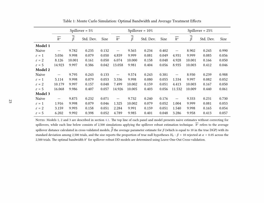
Table 1: Monte Carlo Simulation: Optimal Bandwidth and Average Treatment Effects

Spillover = 5% Spillover = 10% Spillover = 25%

h∗ β Std. Dev. Size h∗ β Std. Dev. Size h∗ β Std. Dev. Size

Model 1

Naive — 9.782 0.235 0.132 — 9.565 0.234 0.402 — 8.902 0.245 0.990ε = 1 5.036 9.998 0.079 0.050 4.859 9.999 0.081 0.049 4.931 9.999 0.085 0.056ε = 2 8.126 10.001 0.161 0.050 6.074 10.000 0.158 0.048 4.928 10.001 0.166 0.050ε = 5 14.923 9.997 0.386 0.042 13.058 9.981 0.404 0.056 8.935 10.003 0.412 0.046Model 2

Naive — 9.795 0.243 0.133 — 9.574 0.243 0.381 — 8.930 0.239 0.988ε = 1 5.114 9.998 0.079 0.053 3.336 9.998 0.080 0.055 1.534 9.997 0.082 0.052ε = 2 10.179 9.997 0.157 0.048 7.499 10.002 0.159 0.051 4.413 10.003 0.167 0.050ε = 5 16.068 9.986 0.407 0.057 14.926 10.005 0.403 0.056 11.532 10.009 0.440 0.061Model 3

Naive — 9.875 0.232 0.071 — 9.732 0.240 0.176 — 9.333 0.231 0.730ε = 1 1.916 9.998 0.079 0.046 1.325 10.002 0.079 0.052 1.004 9.999 0.081 0.053ε = 2 3.159 9.993 0.158 0.051 2.284 9.991 0.159 0.051 1.540 9.998 0.165 0.054ε = 5 6.202 9.992 0.398 0.052 4.789 9.985 0.401 0.048 3.286 9.958 0.413 0.057

Notes: Models 1, 2 and 3 are described in section 4.1. �e top line of each panel and model presents naive estimates without correcting for

spillovers, while each line below consists of 2,500 simulations applying the spillover robust estimation technique. h∗ refers to the average

spillover distance calculated in cross-validated models, β the average parameter estimate for β (which is equal to 10 in the true DGP) with its

standard deviation among 2,500 trials, and the size reports the proportion of true null hypotheses H0 : β = 10 rejected at α = 0.05 across the

2,500 trials. �e optimal bandwidth h∗ for spillover-robust DD models are determined using Leave-One-Out Cross-validation.

23

Finally, it is important to note that while RMSE calculated using LOOCV leads to (generally) cor-

rectly captured spillover bandwidths, and estimated treatment effects with good size properties, in

certain cases the use of LOOCV will be computationally infeasible, specifically as the number of ob-

servations grows. In these cases, k-fold CV offers a computationally convenient alternative manner to

calculate h∗. We document in Appendix Figure A2 and Appendix Table A1, that the use of k-fold CV

results in identical optimal spillover bins, even if calculations of the RMSE are generally higher when

generated using k-fold CV, given that predictions are made using fewer training observations. Further-

more, when considering the parameters estimated using k-fold, rather than LOO, CV we find largely

similar results in terms of size and estimated parameters. �ese are fully documented in Appendix

Table A1, where performance is qualitatively identical. We demonstrate a case where k-fold CV is of

considerable use below in an extended empirical example.

4.2 An Applied Example: Test Messaging Bans and Local Spillovers over

Roadways

In order to examine the performance of the spillover-robust DD strategy in an applied se�ing we con-

sider estimates from an existing DD study, in which only headline treatment are estimated, but in which

propagation of treatment over space may plausibly occur. To do this, we revisit the results of Abouk

and Adams (2013), who examine the passage of state-level laws in the US prohibiting the sending of text

messages while driving. While Abouk and Adams (2013) document a range of impacts of these laws

on rates of deaths in Single Vehicle Single Occupant (SVSO) accidents in a DD se�ing, they restricted

their a�ention only to the impacts on accidents occurring in the same states in which reforms were

implemented.

Nevertheless, there is reason to suspect that laws of this type will not be uniquely restricted to the

states where they are passed. If drivers do actually alter their behaviour in the presence of the law,

it is plausible that their behaviour may not immediately revert to be what it would have been in the

absence of the law when driving across state boundaries. In particular, there are various outcomes

which may be observed. Firstly, it is possible that drivers who are convinced by the state law to reduce

the usage of mobile phones when driving will maintain their improved behaviour when crossing into

nearby states, with perceptible reductions in mortality on roadways also in areas close to the borders of

treated states. Alternatively, an unintended behaviour may be observed, where the law simply causes

inter-state drivers to hold-off on using their mobile phone when driving until they cross into areas

without a law, meaning that any estimates of the reform’s impact using fatal accidents in-state actually

overstates the true impact. �ese two potential behaviours work in opposite directions, suggesting

that the actual impact of reforms may be either over or understated, implying that the estimation of

24

spillover robust DD models allows for the resolution of an empirically relevant policy and behavioural

question.

Abouk and Adams (2013) collect data on all text-messaging bans passed into state law between 2007

and 2010, and use data on all fatal accidents over this period from the Fatality Analysis Reporting System

(FARS) of the National Highway Traffic Safety Administration. �ey also classify text-messaging bans

into two broad classes: weak or strong, which depends on whether text-messaging is a primary (strong)

or secondary offense or restricted to young drivers (weak).13 In the original paper the authors collapse

accidents to state bymonth cells, for 48months (Jan 2007-Dec 2010) for 49 states (Alaska is removed due

to missing data). �e original paper estimates DDmodels focusing on the rate of accidents by state, and

the impact of the different text-messaging bans. In order to examine the occurrence of local spillovers,

we consider the impact on a county-by-county basis here. �is permits for a much finer analysis of the

distance to treatment. In Appendix Table A2 we provide the original (state-level) summary statistics

of dependent and independent variables from Abouk and Adams (2013), and below identical variables

collected at a county-level. Appendix Figure A3 documents the geographic distribution of all accidents

along with state and county boundaries. In Appendix Table A3 we replicate their full DD analysis at the

county-level, finding largely identical results, and in Appendix Table A4 we show simple DD models

without yet considering for the presence of spillovers at both the original (state) level in panel A, and

the new (county) level in panel B.

Figure 2 displays the states which at any point pass different types of text-messaging bans during the

period under study, as well as the distance to treatment from each (un-treated) county in the mainland

US.�ese distances refer to the average distance from each county to the nearest treated state border.14

Wepresent treatment status aswell as distance to treatment for each of the three types of textmessaging

bans considered in Abouk and Adams (2013): handheld bans in panel 2b, primarily-enforced bans in

panel 2c, and secondarily-enforced bans in panel 2d, as well as the distance to any type of ban in panel

2a. �e original list of states enacting test messaging bans along with the date of enactment, as well as

the type of ban enacted can be found in Table 1 of Abouk and Adams (2013). �e distance from each

county displayed in Figure 2 is calculated in kilometres, ranging from 0 km (treated) to greater than

500 km. While it seems extremely unlikely that any impact of the bans would propagate even as much

as 100 km from a treated state into nearby counties, we show distances up to 500 km to demonstrate

that even if spillovers travelled for as much as 500 km, then there would still be additional untreated

13Classification as a primary offense allows for suspected drivers to be pulled over even if no other crime has beencommi�ed, while secondary offenses do not allow this. Further discussion is provided in Abouk and Adams (2013, pp.183–184).

14In this case, the relevant distance is based on travelling over roads from the nearest treated state, and so closest stateborders are used as a manner to capture distance from the nearest area where drivers will be directly affected by laws, ratherthan mid-point to mid-point distances, or alternative distance measures. In code distributed along with this paper, we alsoprovide routines to find travel distance from point to point over roads, as well as average travel times in cars.

25

states for each case. �is is a fundamental assumption for the spillover-robust DD method, where we

require that SUTVA hold between at least some units.

Figure 2: Distances between Counties and Treatment States

>500.00

400.00 − 500.00

300.00 − 400.00

200.00 − 300.00

100.00 − 200.00

0.00 − 100.00

0.00 − 0.00

Distance

(a) All Texting Bans

>500.00

400.00 − 500.00

300.00 − 400.00

200.00 − 300.00

100.00 − 200.00

0.00 − 100.00

0.00 − 0.00

Distance

(b) Handheld Bans

>500.00

400.00 − 500.00

300.00 − 400.00

200.00 − 300.00

100.00 − 200.00

0.00 − 100.00

0.00 − 0.00

Distance

(c) Strong Bans

>500.00

400.00 − 500.00

300.00 − 400.00

200.00 − 300.00

100.00 − 200.00

0.00 − 100.00

0.00 − 0.00

Distance

(d) Weak Bans

Notes to figure 2: Each panel displays distances of each county to the nearest treatment state once all bans have beenenacted. States indicated in red are those treated in each case. Panel (a) displays distances to any types of bans, panel(b) displays cases with a universal concurrent hand-held ban, panel (c) displays only bans with primary enforcement, andpanel (d) displays bans only with secondary enforcement. Distances are displayed by county, based on the distance fromthe centre of each county to the closest point on the border of the closest treated state.

We extend the results of Abouk and Adams (2013) to consider spillovers, in each case following

precisely their variable measurement, controls, estimation sample, and probability weights, however at

the county level, rather than the state level. �us, the baseline DD specification for each type of ban is,

following their equation 1:

Yim = α + γi + δm +Ximβ + ωBim + εim (22)

where Yim refers to the log number of accidents + 1 for county i and monthm, γ a series of county fixed

effects (for the 3,111 counties of the 49 states used in the original analysis), and δm fixed effects for the 48

months of data. County by month cells are weighted by county population, and additional controlsXim

follow the original analysis. In column 1 of Table 2 we present estimates of ω from equation 22 with

naive models assuming that no spillovers occur. �ese estimates are presented for each of the three

26

different types of bans discussed above, and suggest, as in Abouk and Adams (2013), that strong bans

reduce the rate of fatalities occurring in SVSO accidents (in this case by approximately 6%), whereby

weak bans appear to be worse than having no ban in place at all (a significant 7% increase in fatalities

is observed following the introduction of weak bans). While Abouk and Adams (2013) focus largely on

the results of strong bans, they do suggest that the introduction of weak bans may be a result of higher

pre-ban rates of accidents. In the case of the introduction of handheld mobile telephone bans, baseline

DD models do not find statistically significant reductions in accidents following their introduction,

although the direction of the effect is negative, and the magnitude quite large, generally supporting

Abouk and Adams (2013)’s finding of a negative effect of handheld bans.

In turning to spillovers, we implement the spillover robust DD methodology in the remaining

columns of Table 2. In this table the distance bins over which spillovers are estimated is arbitrarily

set at h = 10. �is first approximation allows us to examine spillovers in a general way, before we turn

to the non-arbitrary optimising formula in Table 3. In this first take, we do observe that spillovers are

a relevant phenomenon in this case, and that spillovers are always of the same direction as the reform

itself. �is suggests that if drivers do alter behaviour in response to reforms, these behavioural changes

are not immediately undone at state borders, but rather, seem to perdure in neighbouring and nearby

counties.

In the case of weak bans and handheld bans, significant impacts of the text messaging bans are ob-

served in neighbouring areas, while for strong bans, we do not find evidence to suggest that spillovers

occur, at least when bandwidths are set at 10km. In general there is evidence that when these spillovers

exist, they fade out over a relatively short distance. For the case of weak bans, effects appear to be sig-

nificant from [0-10), [10,20), and [20,30) km, but then no longer remain distinguishable between [30,40)

km, while in the case of handheld bans, spillovers are observed up to 10km, but then not a�er, with the

exception of one coefficient above 30km. In each case, when spillovers are observed in nearby areas,

we observe that controlling for these spillovers increases the magnitude of the treatment effect itself, as

is demonstrated in the calculation of the bias in treatment effects derived in equation 18. Considering

spillovers for both weak and handheld bans increases the magnitude of point estimates, however in no

case are the estimated differences in treatment effects themselves statistically distinguishable across

models. �is points to an important result in the derived bias of spillover effects. Where spillovers

occur only very locally, even if the effect of spillovers is large, given that spillovers only reach a very

small pool of the full original control group, these do not result in large swings in the original treatment

effects estimator. Nonetheless, in both weak and handheld bans, naive models do fail to identify sig-

nificant treatment effects on the close to treated—a relevant consideration when determining the total

effect of a policy.

While se�ing the bandwidth at 10 km does suggest the spillovers are present, an advantage of the

27

Table 2: Reform and Spillover Effects: Bins in 10km

(1) (2) (3) (4) (5)

Panel A: Strong Ban

Strong Ban -0.062** -0.062** -0.061** -0.062** -0.062**

[0.027] [0.027] [0.027] [0.026] [0.026]

Close to strong ban [0-10)km -0.004 -0.003 -0.005 -0.005

[0.048] [0.049] [0.050] [0.051]

Close to strong ban [10-20)km 0.024 0.024 0.023

[0.036] [0.037] [0.037]

Close to strong ban [20-30)km -0.015 -0.016

[0.032] [0.033]

Close to strong ban [30-40)km -0.026

[0.049]

Panel B: Weak Ban

Weak Ban 0.073*** 0.073*** 0.075*** 0.076*** 0.075***

[0.019] [0.019] [0.019] [0.019] [0.020]

Close to weak ban [0-10)km 0.071*** 0.072*** 0.073*** 0.073***

[0.017] [0.017] [0.017] [0.018]

Close to weak ban [10-20)km 0.047* 0.048* 0.047*

[0.024] [0.024] [0.025]

Close to weak ban [20-30)km 0.061** 0.060**

[0.025] [0.026]

Close to weak ban [30-40)km -0.033

[0.070]

Panel C: Handheld Ban

Handheld Ban -0.073 -0.076 -0.076 -0.075 -0.075

[0.048] [0.047] [0.047] [0.048] [0.048]

Close to handheld ban [0-10)km -0.094** -0.094** -0.093** -0.093**

[0.044] [0.044] [0.045] [0.046]

Close to handheld ban [10-20)km 0.001 0.002 0.001

[0.038] [0.039] [0.039]

Close to handheld ban [20-30)km 0.030 0.029

[0.024] [0.024]

Close to handheld ban [30-40)km -0.099*

[0.058]

Observations 149328 149328 149328 149328 149328

Notes: Each panel presents a separate difference-in-differencesmodel with progressive controls capturing

time-varying distance to treatment. Distances are arbitrarily split into bands of 10km. Controls follow the

specifications described in Abouk and Adams (2013) exactly. Standard errors are clustered by state, and

observations are weighted by county population. Each specification includes county by state fixed effects

and month by year fixed effects. �e dependent variable is the natural logarithm of fatal accidents + 1.

28

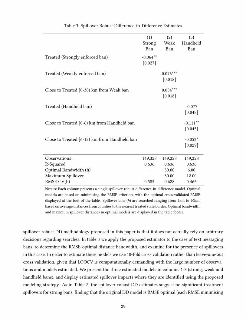
Table 3: Spillover Robust Difference-in-Difference Estimates

(1) (2) (3)Strong Weak HandheldBan Ban Ban

Treated (Strongly enforced ban) -0.064**

[0.027]

Treated (Weakly enforced ban) 0.076***

[0.018]

Close to Treated [0-30) km from Weak ban 0.054***

[0.018]

Treated (Handheld ban) -0.077

[0.048]

Close to Treated [0-6) km from Handheld ban -0.111**

[0.045]

Close to Treated [6-12) km from Handheld ban -0.053*

[0.029]

Observations 149,328 149,328 149,328

R-Squared 0.636 0.636 0.636

Optimal Bandwidth (h) — 30.00 6.00

Maximum Spillover — 30.00 12.00

RMSE CV(h) 0.585 0.628 0.465

Notes: Each column presents a single spillover-robust difference-in-difference model. Optimal

models are based on minimising the RMSE criterion, with the optimal cross-validated RMSE

displayed at the foot of the table. Spillover bins (h) are searched ranging from 2km to 40km,

based on average distances from counties to the nearest treated state border. Optimal bandwidth,

and maximum spillover distances in optimal models are displayed in the table footer.

spillover robust DD methodology proposed in this paper is that it does not actually rely on arbitrary

decisions regarding searches. In table 3 we apply the proposed estimator to the case of text messaging

bans, to determine the RMSE-optimal distance bandwidth, and examine for the presence of spillovers

in this case. In order to estimate these models we use 10-fold cross validation rather than leave-one-out

cross validation, given that LOOCV is computationally demanding with the large number of observa-

tions and models estimated. We present the three estimated models in columns 1-3 (strong, weak and

handheld bans), and display estimated spillover impacts where they are identified using the proposed

modeling strategy. As in Table 2, the spillover-robust DD estimates suggest no significant treatment

spillovers for strong bans, finding that the original DD model is RMSE optimal (each RMSE minimising

29

bandwidth, as well as the RMSE itself is displayed at the foot of the table). For weak bans and handheld

bans, optimal bandwidths are determined to be 30 km and 6 km respectively. When using a bandwidth

of 30 km for weak bans we observe a single close to treated group in which spillovers are estimated to

be significant, suggesting that the reform impacts propagated up to 30km from treatment. In the case

of handheld bans, the 6 km bandwidth results in two perceptible spillover bins with estimated impacts

of decreasing magnitude, suggesting that the impact of reforms may spread up to 12 km from the orig-

inally treated states. While the point estimate on handheld bans increases in magnitude and moves

in the direction of becoming statistically significant (p-value ≈ 0.11), it does not become significant at

frequently used significance levels. In considering only the point estimates on weak bans and handheld

bans, the estimated impact of the reform increases by 4.1 and 5.5% respectively, however, as discussed

above, given that spillovers occur to a relatively small proportion of the total original control group,

these differences are not statistically distinguishable between models.

5 Conclusion

Echoing Bertrand et al. (2004), “Differences-in-Differences (DD) estimation has become an increasingly

popular way to estimate causal relationships”. It is important to consider the assumptions underlying

these estimators. �ere is now a broad literature examining assumptions relating to inferencewhich can

account for the serial correlation in outcomes over time in DD se�ings (Bertrand et al., 2004; Cameron

et al., 2008; Cameron and Miller, 2015) as well as a necessary (but not sufficient) test for the valid-

ity of parallel trend assumptions (Borusyak and Jaravel, 2016), and manners to proceed when these

assumptions are not met (Abadie et al., 2010; Doudchenko and Imbens, 2016)

In this paper we turn to examine the performance of DD estimates when the stable unit treatment

value assumption does not hold locally. We document, firstly, how to determine if SUTVA is violated

by local spillovers (which depend monotonically on distance to treatment), and secondly provide a

convenient closed-form expression for determining the bias in models where treatment spillovers do

occur. We finally derive a set of conditions by which DD estimates can produce unbiased estimates

even in the absence of the SUTVA holding between all units. It is shown that under a weaker set of

conditions, both the average effect on the treated and the average effect on the ‘close to treated’ can be

estimated in a DD-type framework.

�e frequency of papers in the economics literature estimating difference-in-difference models

where treatment access varies within countries suggests that local spillovers may o�en be a relevant

consideration. Such a situation may be particularly common in estimates of the causal effect of policy

where compliance is imperfect. If policies entail a benefit to recipients, and if recipients living ‘close

30

to’ treatment areas who are themselves untreated can somehow cross regional boundaries to receive

treatment, we may be concerned that, locally at least, SUTVA is violated.

In this paper we examine a particular empirical example where geographic dependence of treatment

seems likely. Focusing on text messaging bans, it is suggested that if driving behaviour is altered in

the presence of state-level laws, it may not immediately revert when crossing into contiguous states

(and counties) where no bans are in place. We observe that such a behavioural response to laws occurs.

In particular, we observe that behavioural changes resulting from laws seem to perdure, rather than

observe that text messaging is simply delayed until traveling on roads in nearby untreated areas. �ese

estimates suggest that both consideration of average treatment effects on the treated, as well as average

treated effects on the close to treated, are relevant when determining the impacts of local policies.

What’s more, while we observe that correcting for spillovers does increase the magnitude of estimated

average treatment effects on the treated, in the case examined these differences are not large enough

to be statistically distinguishable from baseline estimates, in line with the intuition behind the nature

of biases in estimates in DD models. I show, both formally in derivations of the omi�ed variable bias,

and in a series of Monte Carlo simulations, that failure to account for spillovers in DD models becomes

increasingly expensive in terms of the performance of the estimator for two reasons. Firstly, estimates

suffer more when the impact of receiving spillover access to a policy on the outcome of interest is larger,

and, secondly as spillover effects propagate to a larger portion of the untreated population.

�is paper provides an optimising and deterministic way to estimate treatment effects as well as

spillover effects in DD models. �e proposed estimator does not require any ad-hoc or arbitrary speci-

fication decisions to be made by researchers. �ese tests are easy to run, and indeed a so�ware package

that automates this methodology in various languages is released with this paper. Given the nature of

the assumptions underlying identification in many DD models in the applied econometric literature,

tests of this nature should be included in a basic suite of falsification tests even if spillovers are not

likely to occur, though will clearly be most illustrative in policy analysis when treatment spillover is a

relevant phenomenon. While the example in this paper is illustrated using geographic spillovers over

roads, spillover-robust DD estimation is certainly not limited to only geographic cases, also occurring

in other family or social networks, such as contagion between peers in school, access to information in

a network, ideological distance to different media sources, and so forth. How (and whether) treatment

travels between units should be of fundamental concern to many applications in the economic and

policy evaluation literature.

31

References

A. Abadie. Semiparametric Difference-in-Differences Estimators. Review of Economic Studies, 72(1):

1–19, 2005.

A. Abadie, A. Diamond, and J. Hainmueller. Synthetic Control Methods for Comparative Case Studies:

Estimating the Effect of California’s Tobacco Control Program. Journal of the American Statistical

Association, 105(490):493–505, 2010.

R. Abouk and S. Adams. Texting Bans and Fatal Accidents on Roadways: Do�eyWork? Or Do Drivers

Just React to Announcements of Bans? American Economic Journal: Applied Economics, 5(2):179–199,

2013.

H. Allco� and D. Keniston. Dutch Disease or Agglomeration? �e Local Economic Effects of Natural

Resource Booms in Modern America. �e Review of Economic Studies, –(–):– – –, forthcoming.

D. Almond, L. Edlund, andM. Palme. Chernobyl’s Subclinical Legacy: Prenatal Exposure to Radioactive

Fallout and School Outcomes in Sweden. �e�arterly Journal of Economics, 124(4):1729–1772, 2009.

M. Angelucci and G. D. Giorgi. Indirect Effects of an Aid Program: How Do Cash Transfers Affect

Ineligibles’ Consumption? American Economic Review, 99(1):486–508, March 2009.

M. Angelucci and V. D. Maro. Program Evaluation and Spillover Effects. SPD Working Papers 1003,

Inter-American Development Bank, Office of Strategic Planning and Development Effectiveness

(SPD), May 2010.

P. M. Aronow and C. Samii. Estimating Average Causal effects under General Interference, with Ap-

plication to a Social Network Experiment. Annals of Applied Statistics, –(–):— – —, forthcoming.

O. Ashenfelter and D. Card. Using the Longitudinal Structure of Earnings to Estimate the Effects of

Training Programs. Review of Economics and Statistics, 67(4):648–660, November 1985.

S. Baird, A. Bohren, C. McIntosh, and B. Ozler. Optimal Design of Experiments in the Presence of

Interference. �e Review of Economics and Statistics, -(-):– – –, forthcoming.

R. Benabou. Workings of a City: Location, Education, and Production. �e �arterly Journal of Eco-

nomics, 108(3):619–652, 1993.

M. Bertrand, E. Duflo, and S. Mullainathan. How Much Should We Trust Differences-in-Differences

Estimates? �arterly Journal of Economics, 119(1):249–275, February 2004.

32

L. E. Blume, W. A. Brock, S. N. Durlauf, and Y. M. Ioannides. Identification of Social Interactions. In

J. Benhabib, A. Bisin, and M. Jackson, editors, Handbook of Social Economics, volume 1, chapter 18,

pages 853–964. Elsevier, June 2011.

K. Borusyak and X. Jaravel. Revisiting event study designs. Working paper, 2016. URL http://

papers.ssrn.com/sol3/papers.cfm?abstract id=2826228.

W. A. Brock and S. N. Durlauf. Discrete Choice with Social Interactions. �e Review of Economic Studies,

68(2):235–260, 2001.

A. C. Cameron and D. L. Miller. A practitioner’s guide to cluster-robust inference. �e Journal of Human

Resources, 50(2):317–72, 2015.

A. C. Cameron, J. B. Gelbach, and D. L. Miller. Bootstrap-based improvements for inference with clus-

tered errors. �e Review of Economics and Statistics, 90(3):414–427, August 2008.

D. R. Cox. Planning of Experiments. John Wiley & Sons Inc., New York, New York, 1958.

B. Crepon, E. Duflo, M. Gurgand, R. Rathelot, and P. Zamora. Do Labor Market Policies have Dis-

placement Effects? Evidence from a Clustered Randomized Experiment. �e �arterly Journal of

Economics, 128(2):531–580, 2013.

C. de Chaisemartin and X. D’Haultfoeuille. Fuzzy Differences-in-Differences. �e Review of Economic

Studies, –(-):– – –, forthcoming.

N. Doudchenko and G.W. Imbens. Balancing, Regression, Difference-In-Differences and Synthetic Con-

trol Methods: A Synthesis. Working Paper 22791, National Bureau of Economic Research, October

2016.

J. J. Heckman and E. Vytlacil. Structural Equations, Treatment Effects, and Econometric Policy Evalu-

ation. Econometrica, 73(3):669–738, 05 2005.

M. G. Hudgens and M. E. Halloran. Toward Causal Inference with Interference. Journal of the American

Statistical Association, 103(482):832–842, 2008.

G. Imbens and T. Lemieux. Regression discontinuity designs: A guide to practice. Journal of Economet-

rics, 142(2):615–635, 2008.

L. Liu and M. G. Hudgens. Large Sample Randomization Inference of Causal Effects in the Presence of

Interference. Journal of the American Statistical Association, 109(505):288–301, 2014.

T.-T. Lu and S.-H. Shiou. Inverses of 2 × 2 Block Matrices. Computers & Mathematics with Applications,

43(1–2):119–129, 2002.

33

J. Ludwig and D. Miller. Does head start improve children’s life chances? Evidence from a regression

discontinuity design. �arterly Journal of Economics, 122(1):159–208, 2007.

C. F. Manski. Identification of treatment response with social interactions. �e Econometrics Journal,

16(1):S1–S23, February 2013.

C. McIntosh. Estimating Treatment Effects from Spatial Policy Experiments: An Application to Ugan-

dan Microfinance. �e Review of Economics and Statistics, 90(1):15–28, February 2008.

E. Miguel and M. Kremer. Worms: Identifying Impacts on Education and Health in the Presence of

Treatment Externalities. Econometrica, 72(1):159–217, 01 2004.

H. S. Najafi, S. A. Edalatpanah, and G. A. Gravvanis. An efficient method for computing the inverse of

arrowhead matrices. Applied Mathematics Le�ers, 33(1):1–5, 2014.

P. R. Rosenbaum. Interference Between Units in Randomized Experiments. Journal of the American

Statistical Association, 102(477):191–200, 2007.

D. B. Rubin. Estimating Causal Effects of Treatments in Randomized and Nonrandomized Studies.

Journal of Educational Psychology, 66(5):688–701, 1974.

D. B. Rubin. Bayesian Inference for Causal Effects: �e Role of Randomization. �e Annals of Statistics,

6(1):34–58, January 1978.

D. B. Rubin. Randomization Analysis of Experimental Data: �e Fisher Randomization Test Comment.

Journal of the American Statistical Association, 75(371):591–593, September 1980.

M. E. Sobel. What Do Randomized Studies of Housing Mobility Demonstrate?: Causal Inference in the

Face of Interference. Journal of the American Statistical Association, 101(476):1398–1407, 2006.

E. J. Tchetgen Tchetgen and T. J. VanderWeele. On causal inference in the presence of interference.

Statistical Methods in Medical Research, 21(1):55–75, 2010.

T. Zajonc. Boundary Regression Discontinuity Design. Dissertation, Harvard University, May 2012.

A. Zellner. An efficient method of estimating seemingly unrelated regressions and tests for aggregation

bias. Journal of the American Statistical Association, 57(298):348–368, June 1962.

34

Appendix Figures and Tables

Figure A1: Root Mean Squared Error and Bandwidth Search Varying Degree of Spillovers

1 3 5 7 9 11 13 15 17 19 21 23 25

0.9

0.95

1

1.05

1.1

1.15

1.2

1.25

Bandwidth (h)

RMSECV(h)

minh

RMSE CV (h) = 1.0021

argminh

RMSE CV (h) = 5

Single Simulation

Average

(a) DGP 1 (5% Spillovers)

1 3 5 7 9 11 13 15 17 19 21 23 25

0.9

0.95

1

1.05

1.1

1.15

1.2

1.25

Bandwidth (h)

RMSECV(h)

minh

RMSE CV (h) = 1.003

argminh

RMSE CV (h) = 5

Single Simulation

Average

(b) DGP 1 (10% Spillovers)

1 3 5 7 9 11 13 15 17 19 21 23 25

0.9

1

1.1

1.2

1.3

1.4

1.5

Bandwidth (h)

RMSECV(h)

minh

RMSE CV (h) = 1.0042

argminh

RMSE CV (h) = 5

Single Simulation

Average

(c) DGP 1 (25% Spillovers)

1 3 5 7 9 11 13 15 17 19 21 23 25

0.95

1

1.05

1.1

1.15

1.2

1.25

Bandwidth (h)

RMSECV(h)

minh

RMSE CV (h) = 1.0093

argminh

RMSE CV (h) = 4

Single Simulation

Average

(d) DGP 2 (5% Spillovers)

1 3 5 7 9 11 13 15 17 19 21 23 25

0.9

0.95

1

1.05

1.1

1.15

1.2

1.25

Bandwidth (h)

RMSECV(h)

minh

RMSE CV (h) = 1.0085

argminh

RMSE CV (h) = 2

Single Simulation

Average

(e) DGP 2 (10% Spillovers)

1 3 5 7 9 11 13 15 17 19 21 23 25

0.9

1

1.1

1.2

1.3

1.4

1.5

Bandwidth (h)

RMSECV(h)

minh

RMSE CV (h) = 1.0111

argminh

RMSE CV (h) = 1

Single Simulation

Average

(f) DGP 2 (25% Spillovers)

1 3 5 7 9 11 13 15 17 19 21 23 25

0.9

0.95

1

1.05

1.1

1.15

1.2

1.25

1.3

Bandwidth (h)

RMSECV(h)

minh

RMSE CV (h) = 1.0106

argminh

RMSE CV (h) = 2

Single Simulation

Average

(g) DGP 3 (5% Spillovers)

1 3 5 7 9 11 13 15 17 19 21 23 25

0.9

1

1.1

1.2

1.3

1.4

1.5

Bandwidth (h)

RMSECV(h)

minh

RMSE CV (h) = 1.0097

argminh

RMSE CV (h) = 1

Single Simulation

Average

(h) DGP 3 (10% Spillovers)

1 3 5 7 9 11 13 15 17 19 21 23 25

0.9

1

1.1

1.2

1.3

1.4

1.5

1.6

1.7

1.8

1.9

Bandwidth (h)

RMSECV(h)

minh

RMSE CV (h) = 1.0114

argminh

RMSE CV (h) = 1

Single Simulation

Average

(i) DGP 3 (25% Spillovers)

Notes to figure A1: Refer to Figure 1 for full notes. Here we provide full RMSE plots for a range of degree of spillovers. �ethree figures in the le�-hand column are based on 5% of the sample being affected by spillovers (for each of the three DGPsexamined), the middle column are based on 10% spillovers (reproduced for comparison from Figure 1), and the right-handpanel are based on 25% of the sample being impacted by spillovers.

35

Figure A2: Root Mean Squared Error Criterion with k-fold versus Leave-One-Out Cross-Validation

1 3 5 7 9 11 13 15 17 19 21 23 25

1

1.05

1.1

1.15

1.2

1.25

1.3

1.35

1.4

Bandwidth (h)

RMSECV(h)

argminh

RMSE Leave-One-Out CV (h) = 5

argminh

RMSE k-fold CV (h) = 5

Leave−One−Out Cross Validation

k−fold Cross−Validation

(a) DGP 1

1 3 5 7 9 11 13 15 17 19 21 23 25

1

1.05

1.1

1.15

1.2

1.25

1.3

1.35

1.4

Bandwidth (h)

RMSECV(h)

argminh

RMSE Leave-One-Out CV (h) = 2

argminh

RMSE k-fold CV (h) = 2

Leave−One−Out Cross Validation

k−fold Cross−Validation

(b) DGP 2

1 3 5 7 9 11 13 15 17 19 21 23 25

1

1.1

1.2

1.3

1.4

1.5

1.6

1.7

1.8

1.9

Bandwidth (h)

RMSE

CV(h)

argminh

RMSE Leave-One-Out CV (h) = 1

argminh

RMSE k-fold CV (h) = 1

Leave−One−Out Cross Validation

k−fold Cross−Validation

(c) DGP 3

Notes to figure A2: Root Mean Squared Error (RMSE) by spillover bandwidth is plo�ed for Leave-One-Out (LOO) cross-validation (line with circles) and k-foldcross-validation (line with squares). �e k-fold cross validation is calculated using 10 folds, where folds are stratified by spillover bins, to allow approximate balance ofspillover variables in each of the k folds. �e optimal bandwidth distance (h∗) for each of the LOOCV and k-fold CV procedure are displayed in each panel of the figure,and DGPs are exactly as shown in identical panels of Figure 1.

36

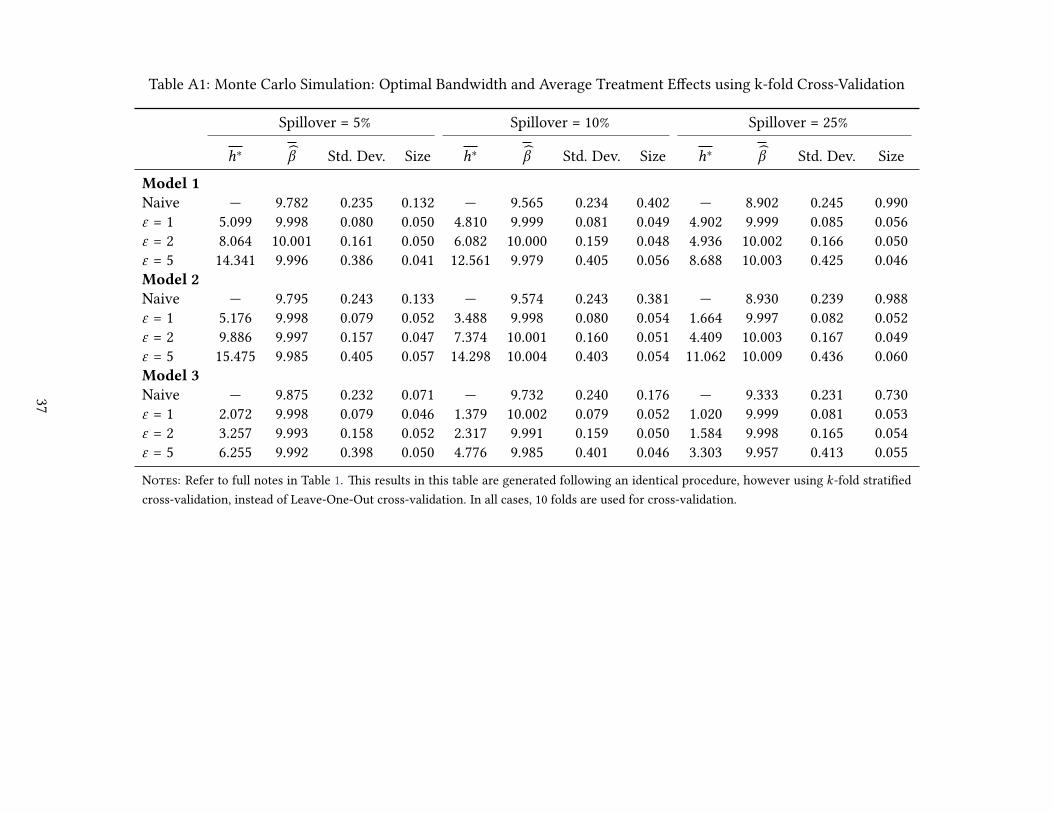
Table A1: Monte Carlo Simulation: Optimal Bandwidth and Average Treatment Effects using k-fold Cross-Validation

Spillover = 5% Spillover = 10% Spillover = 25%

h∗ β Std. Dev. Size h∗ β Std. Dev. Size h∗ β Std. Dev. Size

Model 1

Naive — 9.782 0.235 0.132 — 9.565 0.234 0.402 — 8.902 0.245 0.990ε = 1 5.099 9.998 0.080 0.050 4.810 9.999 0.081 0.049 4.902 9.999 0.085 0.056ε = 2 8.064 10.001 0.161 0.050 6.082 10.000 0.159 0.048 4.936 10.002 0.166 0.050ε = 5 14.341 9.996 0.386 0.041 12.561 9.979 0.405 0.056 8.688 10.003 0.425 0.046Model 2

Naive — 9.795 0.243 0.133 — 9.574 0.243 0.381 — 8.930 0.239 0.988ε = 1 5.176 9.998 0.079 0.052 3.488 9.998 0.080 0.054 1.664 9.997 0.082 0.052ε = 2 9.886 9.997 0.157 0.047 7.374 10.001 0.160 0.051 4.409 10.003 0.167 0.049ε = 5 15.475 9.985 0.405 0.057 14.298 10.004 0.403 0.054 11.062 10.009 0.436 0.060Model 3

Naive — 9.875 0.232 0.071 — 9.732 0.240 0.176 — 9.333 0.231 0.730ε = 1 2.072 9.998 0.079 0.046 1.379 10.002 0.079 0.052 1.020 9.999 0.081 0.053ε = 2 3.257 9.993 0.158 0.052 2.317 9.991 0.159 0.050 1.584 9.998 0.165 0.054ε = 5 6.255 9.992 0.398 0.050 4.776 9.985 0.401 0.046 3.303 9.957 0.413 0.055

Notes: Refer to full notes in Table 1. �is results in this table are generated following an identical procedure, however using k-fold stratified

cross-validation, instead of Leave-One-Out cross-validation. In all cases, 10 folds are used for cross-validation.

37

Table A2: Summary Statistics: State and Municipal-Level

Treatment Areas

Control Areas All months Pre-ban Post-ban

Panel A: State-level Data

Number of single-vehicle single- 16.84 16.13 16.12 16.16occupant accidentsPopulation (annual) 5,157,694 7,064,738.4 6,614,487.1 8,066,043.5Unemployment rate (monthly) 6.51 6.83 6.01 8.63Proportion male (monthly) 49.32 49.34 49.37 49.26Real gas tax in 1983 cents (monthly) 19.94 20.57 20.50 20.73Sample size 1,056 1,296 894 402Panel B: County-level Data

Number of single-vehicle single- 0.2583 0.2597 0.2594 0.2601occupant accidentsPopulation (annual) 79,198.5 113,713 106,437 129,901Unemployment rate (monthly) 6.49 6.99 6.19 8.76Proportion male (monthly) 49.33 49.33 49.39 49.21Real gas tax in 1983 cents (monthly) 19.43 20.27 20.13 20.58Sample size 68,832 80,496 55,533 24,963

Notes: Treatment and control states follow classifications provided in Abouk andAdams (2013). Panel A presents

original state-level data used in difference-in-differences estimates presented in Abouk and Adams (2013). Panel

B presents county-level data used in spillover robust diff-in-diff estimates examined in this paper. All variables

follow precisely the definitions from original analysis.

38

Figure A3: Geographical Distribution of Single Vehicle Single Occupant Accidents

Handheld Device Restriction

Yes

No

39

Table A3: Determinants of Fatal, Single-Vehicle, Single-Occupant Crashes (Municipal data)

(1) (2) (3) (4) (5)

Texting ban in place -0.0229(0.0283)

× universally applied, primarily enforced -0.0525 -0.0519 -0.0471 -0.0321(0.0274) (0.0273) (0.0296) (0.0242)

× limited coverage/enforcement 0.0541∗∗∗ 0.0538∗∗∗ 0.0264 0.0634∗∗

(0.0128) (0.0130) (0.0249) (0.0203)

Log of population 0.4603 0.5280 0.5267 -0.9411 0.6215(0.5645) (0.4889) (0.4880) (0.8854) (0.7593)

Log of unemployment -0.1787∗ -0.1669∗ -0.1623∗ -0.0916∗ 0.0636(0.0716) (0.0708) (0.0697) (0.0401) (0.0851)

Percent male -0.0059 -0.0093 -0.0092 0.0123 -0.0147(0.0191) (0.0109) (0.0109) (0.0155) (0.0155)

Log of gas tax -0.1169 -0.1044 -0.1023 -0.0681 -0.0137(0.0769) (0.0648) (0.0641) (0.0678) (0.0556)

Other accidents 0.0190∗ 0.0231∗ 0.0163∗

(0.0080) (0.0086) (0.0079)Including 48 month fixed effects Yes Yes Yes No YesIncluding differential monthly trend No No No Yes Yesfor all states

Notes to Table A3: Coefficients are reported from weighted least squares regressions, where weights are based on

county population for 3,111 counties over 48 months (following original specifications, Alaska and Hawaii are not

included). �e dependent variable is the natural logarithm of fatal accidents + 1. All specifications include county

by state fixed effects, and standard errors are clustered by state. Specifications follow precisely those of Abouk and

Adams (2013), however with county-level data in place of state-level data. *** Significant at the 1 percent level. **

Significant at the 5 percent level. * Significant at the 10 percent level.

40

Table A4: State and Municipal-Level Baseline Difference-in-Difference Model

(1) (2) (3)

Panel A: State-level Estimates

Strong Ban -0.090***

[0.028]

Weak Ban 0.103**

[0.043]

Handheld Ban -0.048

[0.061]

Observations 2352 2352 2352

R-Squared 0.902 0.902 0.902

Panel B: County-level Estimates

Strong Ban -0.062**

[0.027]

Weak Ban 0.073***

[0.019]

Handheld Ban -0.073

[0.048]

Observations 149328 149328 149328

R-Squared 0.636 0.636 0.636

Notes: Baseline difference-in-difference models with-

out spillover estimates are presented. Panel A presents

state-level models following Abouk and Adams (2013).

Panel B presents identical specifications however at the

county level, and weighted by county, rather than by

states. Both models cluster standard errors by state,

to allow arbitrary correlations among counties within

states across time and across space.

41

A Alternative Methodologies

�e present paper is interested in quantifying the impacts of some externally defined policy of interest,

on individuals in treated areas, and on individuals living in areas close to treatment. �e definition of

the policy itself is assumed to not be under the direct control of the treated and untreated individu-

als themselves. �e se�ing of this paper is thus different to analyses where externalities occur due to

coordination of individual behaviour, and spillovers from social interactions, such as conformation to

reference group behaviour (for example, as in Brock and Durlauf (2001); Benabou (1993)). Consider-

ably extended summaries of the state of the literature of spillover effects and treatment interference

are available in a number of review papers, including Tchetgen Tchetgen and VanderWeele (2010); An-

gelucci and Maro (2010); Blume et al. (2011). Work of Rosenbaum (2007) discusses a number of cases in

which interference between units is observed, and derives non-parametric methods for estimation in

cases in which no information regarding the degree of interference is known.

Generalised Methods �e work of Manski (2013); Aronow and Samii (forthcoming) provide the

most general considerations of social interactions in econometric models. Both of these provide models

allowing for arbitrary forms of interdependence in treatment assignment between individuals, and doc-

ument the identification requirements on treatment effects. When considering the nature of spillovers,

Aronow and Samii (forthcoming) refer to an “exposuremapping”, which describes individual treatments

and the propagation of treatment, while Manski (2013) refers to “effective treatment”, to describe the

same process. Importantly, neither model requires that spillovers are limited to an individual’s refer-

ence group, however such a circumstance is nested in their models. In this paper, I also do not require

spillovers to be isolated to an individual’s reference group, meaning that the method proposed can be

couched in bothManski (2013) or Aronow and Samii (forthcoming)’s terms. �e difference between this

paper and the work of Manski (2013); Aronow and Samii (forthcoming) is that I focus on a particular

type of spillovers, fully specify the manner in which interference occurs, and provide a systematic way

to estimate the degree of interference. �is can thus be considered an estimable application of these

theories to capture geographic spillovers in a difference-in-difference se�ing.

In Manski (2013)’s terms, the model laid out here allows for monotone metric interactions, which

can either be reinforcing (in the same direction as receipt of treatment) or opposing (in the oppo-

site direction of receipt of treatment). �is is generally known as a Semi-Monotone Treatment Re-

sponse model in Manski (2013). �e spillover-robust DD model defined here lays out restrictions to

the shape of the “response function” (the degree to which treatment propagates over space), without

distributional assumption or direction assumptions on this response function. In Aronow and Samii

(forthcoming)’s terms, the spillover-robust DD model proposes a non-parametric “exposure mapping”

42

determining the treatment (and close to treatment) assignment based on any original treatment as-

signment. While Aronow and Samii (forthcoming) propose an exposure mapping which is based on a

generalised propensity score for the likelihood of exposure with restrictions related to maximal prop-

agation based on sample size (their “Local dependence” condition), the exposure mapping described

in the spillover robust DD model proposes an exposure mapping based on distance to treatment (and

potential interactions).

Within but not between groups An alternative series of papers focus on cases where interference

is allowed within, but not between groups. A series of important theoretical results in this case are

given by Hudgens and Halloran (2008); Liu and Hudgens (2014). �ese strategies have a number of

names, such as “partial interference” (Sobel, 2006), “hierarchical treatment assignment”, or “randomised

saturation” designs (Baird et al., forthcoming). �e la�er case is frequently employed in experimental

applications where treatment is randomised first at the level of a cluster, and then to individuals within

the cluster, and individuals within each cluster are permi�ed to interact freely (consider for example

randomised treatment at the level of schools, such as inMiguel and Kremer (2004), local labour markets,

such as in Crepon et al. (2013) or localities, such as in PROGRESA). A comprehensive discussion of

randomised saturation designs and the resulting estimands is provided by Baird et al. (forthcoming).

�emethods discussed in this paper differ fundamentally from these hierarchical or partial interference

designs in that spillovers are assumed to occur between treatment clusters.

Applications Finally, it is important to note that a number of applied studies estimate difference-

in-difference models in which spillovers are posited (and identified). �ese include Miguel and Kre-

mer (2004)’s study on externalities between schools, Almond et al. (2009)’s examination of the spread

of radioactive fallout during a mother’s pregnancy on schooling outcomes, and Allco� and Keniston

(forthcoming) who consider economic spillovers of local natural resource booms. In each case, these

applied papers propose a structurally similar process to the one I lay out here. �e main difference

with these and the present study is that here we (a) document that such an estimation methodology

is unbiased, and (b) provide a non ad-hoc way to choose distance bins to search for spillovers. In the

past, these were chosen by researchers, likely in a way to best capture spillovers or explain modelled

outcomes, but without a formal optimising method. Applications such as these are precisely the sorts

of cases in which spillover-robust DD is likely to be most useful going forward.

43

B Proofs

Proof of Proposition 1. Y (i, t ) is generated according to (1), and from (7), a regression of Y (i, t ) on D(i, t ) and R(i, t ) can

be estimated. It is assumed that we have at a representative sample of size N consisting of {Y (i, t ),D(i, t ),X (i, t ) : i =

1, . . . ,N , t = 0, 1}. By assumption 4A, the assignment rule δ forms R(i, t ) allowing for the estimation of (7). By definition, α

in this regression is equal to:

α = {E[Y (i, 1)|D(i, 1) = 1,R(i, 1) = 0] − E[Y (i, 1)|D(i, 1) = 0,R(i, 1) = 0]}

− {E[Y (i, 0)|D(i, 1) = 1,R(i, 1) = 0] − E[Y (i, 0)|D(i, 1) = 0,R(i, 1) = 0]},

and from assumption 3, each of the expectation terms exists, as there are both fully treated and completely untreated units.

Using the potential outcomes framework, we are free to re-write the above expression as:

α = {E[Y 1(i, 1)|D(i, 1) = 1,R(i, 1) = 0] − E[Y 0(i, 1)|D(i, 1) = 0,R(i, 1) = 0]}

− {E[Y 0(i, 0)|D(i, 1) = 1,R(i, 1) = 0] − E[Y 0(i, 0)|D(i, 1) = 0,R(i, 1) = 0]},

given that only in the case where t = 1 and D(i, 1) = 1 we observe the potential outcome where the individual receives

treatment: Y 1(i). Using the linearity of the expectations operator, this can finally be re-wri�en as:

α = E[Y 1(i, 1) − Y 0(i, 0)|D(i, 1) = 1,R(i, 1) = 0] − E[Y 0(i, 1) − Y 0(i, 0)|D(i, 1) = 0,R(i, 1) = 0].

Now, from assumption 1, we can appeal to parallel trends, and replace the second expectation term in the above ex-

pression with E[Y 0(i, 1) − Y 0(i, 0)|D(i, 1) = 1,R(i, 1) = 0]:

α = E[Y 1(i, 1) − Y 0(i, 0)|D(i, 1) = 1,R(i, 1) = 0] − E[Y 0(i, 1) − Y 0(i, 0)|D(i, 1) = 1,R(i, 1) = 0].

Expanding the expectations operator and cancelling out the second term in each of the above items gives:

α = E[Y 1(i, 1)|D(i, 1) = 1,R(i, 1) = 0] − E[Y 0(i, 1)|D(i, 1) = 1,R(i, 1) = 0].

which finally, once again by the linearity of expectations, can be combined to give α = E[Y 1(i, 1)−Y 0(i, 1)|D(i, 1) = 1,R(i, 1) =

0], which can be rewri�en as α = E[Y 1(i, 1) − Y 0(i, 1)|D(i, 1) = 1] given that D(i, 1) = 1 =⇒ R(i, 1) = 0. Combining (8) and

α = E[Y 1(i, 1) − Y 0(i, 1)|D(i, 1) = 1] we thus have that α = ATT as required.

Turning to the ATC, the same set of steps can be followed for β on the coefficient R(i, t ), however now instead of

assumption 1 we must rely on parallel-trend assumption 2. �is leads to β = E[Y 1(i, 1) − Y 0(i, 1)|R(i, 1) = 0], and from (9)

and the previous expression it holds that that β = ATC . �

Proof of Proposition 2. With the representative sample {Y (i, t ),D(i, t ),X(i, t ) : i = 1, . . . ,N , t = 0, 1}, assumption 4B

implies that X(i, t ) can be R(i, t ) using assignment rule δ . �e remainder of the proof follows the same steps as the proof for

proposition 1. �

44

Derivation of Conditional Correlations for Bias Formula Consider a sample of size N , consisting of

{Y (i, t ),D(i, 1),R(i, 1),D(i, t ),R(i, t ) : i = 1, . . . ,N , t = 0, 1}. Define the number of observations for whom D(i, 1) = 1 as ND ,

and analogously define NR for those observations for whom R(i, 1) = 1. As D(i, 1) and R(i, 1) are mutually exclusive, no

observations can be counted in both ND and NR . Similarly, define NDTand NRT for the number of observations for whom

D(i, t ) = 1 and R(i, t ) = 1, where once again these are mutually exclusive, and mutually exclusive with each of D(i, 1) = 1

and R(i, 1) = 1. Finally, define as NT the quantity of observations in which t = 1. By definition, all observations for which

R(i, t ) = 1 and D(i, t ) = 1 will be counted in NT , but the inverse is not true (ie there are observations counted in NT who

have neither R(i, t ) = 1 nor D(i, t ) = 1.

In order to determine the bias outlined in the paper, we are interested in the correlation between D(i, t ) and R(i, t ),

conditional on D(i, 1), t and a constant term. �e omission of a control for the “close to treated” indicator R(i, t ) also implies

that a similar binary variable R(i, 1) is omi�ed from the model. �e well-known omi�ed variable bias formula gives that:

E[α |X] = α + (X ′X)−1X ′RβR (A1)

where the second term gives the bias in estimated parameters, R refers to the omi�ed {R(i, 1),R(i, t )} indicators, and βR

is the direct effect of these omi�ed factors on the outcome variable of interest. �e matrix X is an N × 4 matrix, with

X = [1 D(i, 1) D(i, t ) t].

Given that X is a Boolean matrix, and various columns are mutually exclusive, we can write X ′X and X ′R as:

(X ′X) =

N ND NDTNT

ND ND 0 0

NDT0 NDT

NDT

NT 0 NDTNT

X ′R = X ′[R(i, 1) R(i, t )] =

NR NRT

0 0

0 0

0 NRT

.

In the X ′R matrix above, only the constant term in X takes values of one when R(i, 1) = 1, hence the first column only

has one non-zero entry, while both the constant and the time dummy t in X take values of 1 when R(i, t ) = 1. Given that

all occurrences of R(i, t ) = 1 are when t = 1, both entries in the second column of X ′R are the sum of all observations for

which R(i, t ) = 1.

In order to calculate the omi�ed variable bias, (X ′X) must be inverted. �is matrix is a symmetric block matrix, and

so can be re-wri�en as:

A =

[A11 A12

A′12 A22

]A−1 =

[B11 B12

B′12 B22

]

where each ofA11, A12 andA22 are the 2× 2 matrices in each corner of (X ′X). Each element of the inverse has the formula

given below (see for example Lu and Shiou (2002)):

B11 = (A11 −A12A−122A

′12)

−1

=1

ND1 (N − NT − ND1 )

[ND −ND

−ND N − NT

](A2)

B22 = (A22 −A′12A

−111A12)

−1

=1

(NT − NDT)

[NTNDT

−1

−1N−ND−NDT

(N−ND−NT )

](A3)

45

B12 = −A−122A

′12(A11 −A12A

−122A

′12)

−1

=

[0 0

− 1N−NT −ND

1N−NT −ND

](A4)

B′12 = −A−1

11A12(A22 −A′12A

−111A12)

−1

=

[0 − 1

(N−ND−NT )

0 1(N−ND−NT )

]. (A5)

�e first line of each expression above is from the inverse formula for 2 × 2 block matrices, while the second line for each

sub-matrix is resolved by linear algebra.15

Based on the above, we combine A2-A5 to form (X ′X)−1, which gives that the inverse is:

1N−NT −ND

− 1N−NT −ND

0 0

− 1N−NT −ND

N−NTND (N−NT −ND ) − 1

N−NT −ND

1N−NT −ND

0 − 1(N−ND−NT )

NTNDT

(NT −NDT)

−1NT −NDT

0 1(N−ND−NT )

−1NT −NDT

N−ND−NDT

(N−ND−NT )(NT −NDT)

. (A6)

and, to complete the first part of the omi�ed variable bias, this is multiplied with (X ′RT ). �is gives (X ′X)−1(X ′R):

1N−NT −ND

− 1N−NT −ND

0 0

− 1N−NT −ND

N−NTND (N−NT −ND ) − 1

N−NT −ND

1N−NT −ND

0 − 1(N−ND−NT )

NTNDT

(NT −NDT)

−1NT −NDT

0 1(N−ND−NT )

−1NT −NDT

N−ND−NDT

(N−ND−NT )(NT −NDT)

NR NRT

0 0

0 0

0 NRT

=

NR

N−NT −ND

NRT

N−NT −ND

− NR

N−NT −ND0

0−NRT

NT −NDT

0NRT

(N−ND−NDT)

(N−ND−NT )(NT −NDT)

.

Here we are concerned with the bias on the parameter α , which corresponds to the third variable of the X matrix:

D(i, t ). Note from the first column of (X ′X)−1(X ′R), that D(i, t ) has no correlation with R(i, 1) conditional on the included

variables. It does, however, have a correlation with R(i, t ). �is bias is then equal to the direct impact of the omi�ed variable

R(i, t ) on y (β), multiplied by the conditional correlation:

β ×−NRT

NT − NDT

, (A7)

giving

E[α |X] = α − β

(NRT

NT − NDT

)(A8)

as stated in equation 15.

If, however, multiple “close to treatment” indicators (and corresponding baseline fixed effects) are included rather than

15Extended calculations are available from the author by request.

46

a single R indicator, all holds as above, however now the X ′R matrix becomes

NR1 · · · NR J NR1T · · · NR JT

0 · · · 0 0 · · · 0

0 · · · 0 0 · · · 0

0 · · · 0 NR1T · · · NR JT

whereR(i, 1) andR(i, t ) have been further split intomutually exclusiveR1(i, 1),R1(i, t ), . . . ,R J (i, 1),R J (i, t ) distance indicators

as in equation 10, and where analogous integers NR1 ,NR1T , . . . ,NR J ,NR JT refer to the number of observations which take

one for a given binary indicator. In this case, the omi�ed variable bias for the parameter α is given as:

E[α |X] = α − β1

(NR1T

NT − NDT

)− · · · − β J

(NR JT

NT − NDT

), (A9)

as stated in equation 16.

Now, if we include an arbitrary number of close controls (and corresponding fixed effects) in the regression model of

interest, forming

Y (i, t ) = µ + τD(i, 1) + γ1R1(i, 1) + · · · + γ JR

J (i, 1) + δt + αD(i, t ) + β1R1(i, t ) + · · · + β JR

J (i, t ) + ε(i, t ),

with omi�ed spillover variables R> J (i, 1),R> J (i, t ), we can write the relevant matrices as:

(X ′X) =

N ND1 NR1 . . . NR J NDTNR1T . . . NR JT NT

ND1 ND1 0 . . . 0 0 0 . . . 0 0

NR1 0 NR1 . . . 0 0 0 . . . 0 0...

......

. . ....

......

. . ....

...

NR J 0 0 . . . NR J 0 0 . . . 0 0

NDT0 0 . . . 0 NDT

0 . . . 0 NDT

NR1T 0 0 . . . 0 0 NR1T . . . 0 NR1T

......

.... . .

......

.... . .

......

NR JT 0 0 . . . 0 0 0 . . . NR JT NR JT

NT 0 0 . . . 0 NDTNR1T . . . NR JT NT

X ′R> J =

NR> JNR> JT

0 0

0 0

0...

0 0

0 0

0 0

0...

0 0

0 NR> JT

.

Here A11 and A22 are arrowhead matrices, and have a known inverse, and A12, A21 have values in the first row and column

respectively, and the remainder of entries are zeroes. �us, each required block of the 2(J + 2)× 2(J + 2) matrix is invertible,

and it is a symmetric 2 × 2 block matrix. We thus follow the procedure described above for calculating the inverse of 2 × 2

block matrices, giving:

B11 = (A11 −A12A−122A

′12)

−1 =

1θ0

1θ0

1θ0

. . . − 1θ0

1θ0

θ0+ND1

θ0ND1

1θ0

. . . − 1θ0

1θ0

1θ0

θ0+NR1

θ0NR1. . . − 1

θ0

......

.... . .

...

− 1θ0

− 1θ0

− 1θ0

. . .θ0+NRJ

θ0NRJ

(A10)

where θ0 = N − NT − ND1 − NR1 − · · · − NR J ,

47

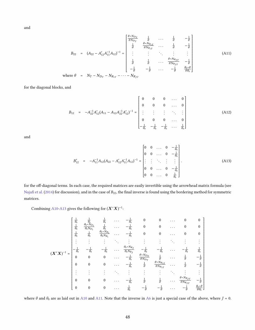
and

B22 = (A22 −A′12A

−111A12)

−1 =

θ+NDT

θNDT

1θ

. . . 1θ

− 1θ

1θ

θ+NR1T

θNR1T. . . 1

θ− 1θ

......

. . ....

...

1θ

1θ

. . .θ+NRJT

θNRJT

− 1θ

− 1θ

− 1θ

. . . − 1θ

θ0+θθθ0

(A11)

where θ = NT − NDT− NR1T − · · · − NR JT

for the diagonal blocks, and

B12 = −A−122A

′12(A11 −A12A

−122A

′12)

−1 =

0 0 0 . . . 0

0 0 0 . . . 0...

......

. . ....

0 0 0 . . . 0

− 1θ0

− 1θ0

− 1θ0. . . 1

θ0

(A12)

and

B′12 = −A−1

11A12(A22 −A′12A

−111A12)

−1 =

0 0 . . . 0 − 1θ0

0 0 . . . 0 − 1θ0

......

. . ....

...

0 0 . . . 0 − 1θ0

0 0 . . . 0 1θ0

. (A13)

for the off-diagonal terms. In each case, the required matrices are easily invertible using the arrowhead matrix formula (see

Najafi et al. (2014) for discussion), and in the case of B22, the final inverse is found using the bordering method for symmetric

matrices.

Combining A10-A13 gives the following for (X ′X)−1:

(X ′X)−1 =

1θ0

1θ0

1θ0

. . . − 1θ0

0 0 . . . 0 01θ0

θ0+ND1

θ0ND1

1θ0

. . . − 1θ0

0 0 . . . 0 0

1θ0

1θ0

θ0+NR1

θ0NR1. . . − 1

θ00 0 . . . 0 0

......

.... . .

......

.... . .

......

− 1θ0

− 1θ0

− 1θ0

. . .θ0+NRJ

θ0NRJ

− 1θ0

− 1θ0

. . . − 1θ0

1θ0

0 0 0 . . . − 1θ0

θ+NDT

θNDT

1θ

. . . 1θ

− 1θ

0 0 0 . . . − 1θ0

1θ

θ+NR1T

θNR1T. . . 1

θ− 1θ

......

.... . .

......

.... . .

......

0 0 0 . . . − 1θ0

1θ

1θ

. . .θ+NRJT

θNRJT

− 1θ

0 0 0 . . . 1θ0

− 1θ

− 1θ

. . . − 1θ

θ0+θθθ0

where θ and θ0 are as laid out in A10 and A11. Note that the inverse in A6 is just a special case of the above, where J = 0.

48

Now, to determine the omi�ed variable bias on each included variable where potentially multiple close to treatment variables

are included and multiple close to treatment variables are excluded, we follow equation A1 which gives the expectation of

α (the estimated average treatment effect), and similarly for each included “close to treatment” variable the expectation of

the estimate is:

E[βk |X] = βk + (X ′X)−1X ′RβR . (A14)

Considering the relevant columns of (X ′X)−1 andX ′R thus results in the following expectations:

E[α |X] = α − βRNR> JT

θ= α − βR

NR> JT

NT − NDT− NRT 1 − . . . − NRT J

(A15)

E[βk |X] = βk − βRNR> JT

θ= α − βR

NR> JT

NT − NDT− NRT 1 − . . . − NRT J

∀k ∈ 1, . . . , J . (A16)

if a single aggregate R> J (i, 1),R> J (i, t ) omi�ed dummy is excluded for additional marginal close to treatment areas, or:

E[α |X] = α − βR+1NR J +1T

θ− βR+2

NR J +2T

θ. . . (A17)

E[βk |X] = βk − βR+1NR J +1T

θ− βR+2

NR J +2T

θ. . .∀k ∈ 1, . . . , J . (A18)

if R> J (i, 1),R> J (i, t ) is further partitioned into multiple “close to treatment” dummies of the form R J+1(i, 1),R J+1(i, t ), . . . ,

RK (i, 1),RK (i, t ). �ese expectations from A17 and A18 are stated in equations 18 and 19 of the paper.

49

C Spillovers as a Nuisance Parameter and Treatment Effect Sta-

bility

If we start by estimating a typical DD specification without controlling for spillovers, our estimated

treatment effect α is given by 16. �is suggests that bias will exist if any spillovers occur beyond the

direct effect of the policy. If spillovers exist below some distance d , then βk 6= 0∀ kh < d , where h

refers to a bandwidth parameter discussed in section 3.1. If this is the case, and if spillovers work in

the same direction as treatment, then |E[α0]|< |α |, implying that the estimated treatment effect will be

a�enuated by treatment spillover to the control group, while if spillover effects work in the opposite

direction of treatment, estimated treatment effects will be over-estimated. In what follows we assume

w.l.o.g. that spillover effects are of the same direction as treatment effects. If the reverse is true, the

below holds simply reversing the direction of convergence of αk to α .

In order to determine the plausibility of spillovers, we can re-estimate our baseline DD model,

however now also condition on R1(i, t ) and R1(i, 1) when estimating α . We refer to this estimate as α1.

Our resulting estimate is displayed in equation 17, and once again, if spillovers exist and are of the

same sign as treatment, then the estimate α1 will be a�enuated, but not as badly as α0 given that we

now partially correct for spillovers up to a distance of h. In this case: |E[α0]|< |E[α1]|< |α |. If, on

the other hand, spillovers do not exist, then we will have that |E[α0]|= |E[α1]|= |α |. �is leads to the

following hypothesis test, where for efficiency reasons α0 and α1 are estimated by seemingly unrelated

regression:

H0 : α0 = α1 H1 : α

0 6= α1.

From Zellner (1962), the test statistic has a χ 21 distribution. If we reject H0 in favour of the alternative,

this indicates that partially correcting for spillovers affects the estimated coefficient α , implying that

spillovers occur at least up to distance h, and that further tests are required.

Rejection of the null suggests that another iteration should be performed, this time adding R1(i, t )

and R2(i, t ) (along with baseline fixed effects) to the model, and the corresponding parameter α2 be

estimated. If spillovers do occur at least up to distance 2h, we expect that |E[α0]|< |E[α1]|< |E[α2]|<

|α |, however if spillovers only occur up to distance h, we will have |E[α0]|< |E[α1]|= |E[α2]|= |α |. �is

leads to a new hypothesis test:

H0 : α1 = α2 H1 : α

1 6= α2,

where the test statistic is distributed as outlined above. Here, rejection of the null implies that spillovers

occur at least up to distance 2h, while failure to reject the null suggests that spillovers only occur up to

distance h.

50

�is process should be followed iteratively up until the point that the marginal estimate αk+1 is

equal to the preceding estimate αk . At this point, we can conclude that units at a distance of at least kh

from the nearest treatment unit are not affected by spillovers, and hence a consistent estimate of α can

be produced. Finally, this leads to a conclusion regarding d and the indicator function R(i, t ) = 1X (i,t )≤d .

When controlling for the marginal distance to treatment indicator no longer affects the estimate of the

treatment effect αk , we can conclude that d = kh, and thus correctly identify R(i, t ) = 1X (i,t )≤kh in data.

51