No 236 – June 2016

Estimating Development Resilience: A Conditional Moments-Based Approach

Jennifer Denno Cissé and Christopher B. Barrett

Editorial Committee

Shimeles, Abebe (Chair) Anyanwu, John C. Faye, Issa Ngaruko, Floribert Simpasa, Anthony Salami, Adeleke O. Verdier-Chouchane, Audrey

Coordinator

Salami, Adeleke O.

Copyright © 2016

African Development Bank

Headquarter Building

Rue Joseph Anoma

01 BP 1387, Abidjan 01

Côte d'Ivoire E-mail: afdb@afdb.org

Rights and Permissions

All rights reserved.

The text and data in this publication may be

reproduced as long as the source is cited.

Reproduction for commercial purposes is

forbidden.

The Working Paper Series (WPS) is produced by the

Development Research Department of the African

Development Bank. The WPS disseminates the

findings of work in progress, preliminary research

results, and development experience and lessons,

to encourage the exchange of ideas and innovative

thinking among researchers, development

practitioners, policy makers, and donors. The

findings, interpretations, and conclusions

expressed in the Bank’s WPS are entirely those of

the author(s) and do not necessarily represent the

view of the African Development Bank, its Board of

Directors, or the countries they represent.

Working Papers are available online at

http:/www.afdb.org/

Correct citation: Cissé, Jennifer Denno and Barrett, Christopher B. (2016), Estimating Development Resilience: A Conditional Moments-Based Approach Working Paper Series N° 236. African Development Bank, Abidjan, Côte d’Ivoire.

Estimating Development Resilience:

A Conditional Moments-Based Approach

Jennifer Denno Cissé* and Christopher B. Barrett

* Jennifer Denno Cissé (Corresponding author. Email: jdc358@cornell.edu) and Christopher B. Barrett are at Charles H. Dyson School of Applied Economics & Management, Cornell University

AFRICAN DEVELOPMENT BANK GROUP

Working Paper No. 236

June 2016

Office of the Chief Economist

Abstract: Despite significant spending on ‘resilience’ by international development agencies, no theory-based method for estimating or measuring development resilience has yet been developed. This paper introduces an econometric strategy for estimating individual or household-level development resilience from panel data. Estimation of multiple conditional moments of a welfare function—itself specified to permit potentially nonlinear path dynamics—enables the computation and forecasting of individual-specific conditional probabilities of satisfying a

normative minimum standard of living. We then develop a decomposable resilience measure that enables aggregation of the individual-specific estimates to targetable subpopulation- and population-level measures. We illustrate the method empirically using household panel data from pastoralist communities in northern Kenya. The results demonstrate not only the method and its potential for targeting resilience-building interventions, but also help explain the behavioral paradox of apparent herd overstocking.

Keywords: Panel data, Poverty dynamics, Resilience, Risk JEL Classification Numbers: C46, I32, O12

5

I. INTRODUCTION

Over the past several years, natural disasters, food price and macroeconomic shocks, and

conflict have prompted recurring humanitarian emergencies in many of the world’s lowest

income countries. In direct response, international development and relief agencies have

become preoccupied with the concept of resilience, committing increasingly large amounts

of funding, programming, and research toward “building resilience.” They struggle,

however, to develop methods to implement the concept empirically so as to guide policy

and project design, measure progress, and evaluate interventions. At the same time, the

concept of development resilience has the potential to draw together the strengths of several

distinct economics literatures on the estimation of stochastic well-being dynamics. The

opportunity is thus ripe for methodological contributions to help advance both operational

and research agendas.

In his seminal work on poverty measurement, Sen (1979) discusses the need for

both poverty “identification” (i.e., determining who is poor) and “aggregation” (i.e.,

establishing how characteristics of the poor can be combined into an aggregate indicator)

to guide policy. The emergent development resilience agenda has similar measurement

needs. Toward that end, we introduce an econometric strategy to estimate individual or

household-level development resilience, so as to identify the targetable characteristics of

those who are (and are not) resilient, and then demonstrate how to aggregate those micro-

level estimates into policy-relevant measures useful for targeting and impact evaluation

purposes. This approach usefully synthesizes the distinct poverty dynamics, risk, and

vulnerability literatures active within economics more broadly.

We follow the Barrett and Constas (2014, p.14626, hereafter BC) conceptualization

of development resilience1 as “the capacity over time of a person, household or other

aggregate unit to avoid poverty in the face of various stressors and in the wake of myriad

1 Although the term is the same, different fields employ different concepts of ‘resilience.’ See Folke (2006)

for a nice review of the concept in the ecology and engineering literatures and Barrett and Constas (2014)

for a discussion of why that concept must be adapted for international development or broader economic

applications.

6

shocks. If and only if that capacity is and remains high over time, then the unit is resilient.”

By couching resilience in terms of stochastic well-being dynamics, BC point towards a

definition that can be implemented empirically. To do so, we draw on the risk literature to

estimate multiple conditional moments of a welfare function specified, following the

poverty traps literature, to include potentially nonlinear path dynamics. Like the

vulnerability literature, the aim is a forward-looking, probabilistic measure of well-being

that can be used for targeting and program evaluation. Then, like the poverty measurement

literature, we demonstrate how the individual-specific estimates can be aggregated into a

decomposable measure useful for policy and operational purposes, such as targeting scarce

resources or evaluating the potentially-heterogeneous impacts of policies and programs on

different sub-populations.

We close by illustrating the method with an empirical example using household

panel data from pastoralist communities in northern Kenya. The results demonstrate the

method’s potential for identifying who is and is not resilient and when, as well as for

generating aggregate measures of development resilience. We also briefly discuss

prospective extensions of this approach to impact evaluation, multidimensional well-being

measures, more sophisticated estimation of the underlying conditional moments, and the

data needs to permit more widespread empirical implementation of such methods.

II. DEVELOPMENT RESILIENCE ESTIMATION

Despite a growing, primarily non-economic, recent literature on development resilience

(e.g., Cannon & Müller-Mahn 2010, Robinson & Berkes 2010, Davoudi 2012, BC, Béné

et al. 2014, Levine 2014), no peer-reviewed measures2 have been proposed and applied

empirically in the development context. The BC approach suggests a path forward based

on integration of several distinct empirical literatures in economics. BC explicitly motivate

their approach from the poverty dynamics and traps literatures that emphasize the

possibility of nonlinear well-being dynamics and asset-based poverty traps (Carter & May

2001; Lybbert et al. 2004; Carter & Barrett 2006; Barrett & Carter 2013; McKay & Perge

2 Several empirical papers have emerged in the grey literature, for example, Alinovi, Mane, & Romano

(2010), Smith et al. (2015), Vaitla et al. (2012), Alfani et al. (2015), and Vollenweider (2015).

7

2013). However, that literature focuses largely on ex post analysis of well-being. The

vulnerability literature (e.g., Christiaensen & Boisvert 2000; Chaudhuri, Jalan, &

Suryahadi 2002; Hoddinott & Quisumbing 2003), on the other hand, emphasizes

probabilistic ex ante measures, although it overlooks the prospective importance of

nonlinear path dynamics. But it is unnecessary to forsake dynamics in order to generate

forward-looking estimates. BC’s definition implies that an economic measure of

development resilience ought to be both probabilistic (building on the vulnerability

literature) and allow for the possibility of nonlinear well-being dynamics (as per the

poverty traps literature). By tapping established methods for estimating conditional

moment functions, as developed in the empirical risk literature (Just & Pope 1979, Antle

1983), we offer an approach to estimating probabilistic ex ante well-being dynamics. Then

by adapting the seminal work of Foster, Greer & Thorbecke (1984, hereafter FGT), we can

turn the individual estimates into aggregate measures decomposable into subgroups that

naturally lend themselves to targeting for policy and project interventions. We emphasize

that none of the component methods we use are original; the novelty of the method arises

from their integration into implementable, theory-based measures of development

resilience.

BC represent development resilience using a conditional moment function for well-

being, specifically 𝑚𝑖𝑘(𝑊𝑖,𝑡+𝑠|𝑊𝑖𝑡, 𝑿𝑖,𝑡+𝑠, 𝜖𝑖,𝑡+𝑠), where 𝑚𝑖

𝑘 is the kth moment of individual

i’s well-being, W, in period t+s (for s>0), a function of well-being in period 𝑡, a set of

individual-, household- and community-level covariates, X, and random disturbances, 𝜖.

An individual’s well-being is therefore considered a random variable, with its own

distribution in each period. One might use any of a host of well-being measures, depending

on the context, from stock measures such as asset holdings or anthropometric indicators of

health status to flow measures such as expenditures or income. The convention in the

empirical poverty traps literature is to estimate only the first moment, the expected path

dynamics of well-being, but to allow for potentially nonlinear path dynamics, as reflected

either in a high-order polynomial in 𝑊𝑡 (Lokshin & Ravallion 2004, Barrett et al. 2006,

Antman & McKenzie 2007) or nonparametric or semiparametric estimation of a first-order

Markov process (Lybbert et al., 2004; Adato, Carter, & May 2006; Naschold 2013). That

8

literature to date has largely ignored heteroscedasticity and other non-constant higher-order

central moments in the estimated path dynamics.

The standard approach in the vulnerability literature, by contrast, is to estimate both

the conditional mean and the conditional variance but to ignore prospective nonlinearity in

the path dynamics by assuming, at best, a linear first-order autoregressive process. The

development and humanitarian agencies’ current focus on resilience originates in the

intersection of vulnerability to shocks and the apparent existence of poverty traps among

the remote (commonly drylands pastoralist) populations on which much of the resilience

discourse focuses. So it seems sensible to take an approach to measurement that integrates

the distinct strengths of each of these two literatures, as BC’s theory allows.

We model the mean (indicated by the M subscript) stochastic well-being of

individual or household i (household hereafter because in our empirical illustration we use

a household-level indicator of well-being) in period t (𝑊𝑖𝑡) parametrically as a polynomial

function (𝑔) of lagged well-being (𝑊𝑖,𝑡−1), and a vector of household characteristics, 𝑿𝒊𝒕,

including shocks directly experienced by i or risks to which i is exposed:

(1) 𝑊𝑖𝑡 = 𝑔𝑀(𝑊𝑖,𝑡−1, 𝑿𝒊𝒕, 𝛽𝑀) + 𝜹𝐌𝑿𝒊𝒕 + 𝑢𝑀𝑖𝑡.

We assume a first-order Markov process for both conceptual and practical reasons.

Conceptually, a lag is necessary to allow for persistence in the impact of previous period

well-being on the future. At the same time, well-being (like wealth) is a state variable which

summarizes all prior states, meaning only one lag is necessary. Empirically, incorporating

a second lag would decrease the number of rounds of panel data available for analysis; the

use of a single lag is economical while also addressing possible autocorrelation in the errors

of the panel data. A cubic specification would be the most parsimonious parametric

specification that allows for the S-shaped dynamics typical of systems characterized by

multiple equilibria poverty traps (Barrett et al. 2006), although higher order polynomials

may be used.

Using 𝐸 to represent the expectation operator, a caret (^) to represent predicted

values, and assuming that the random error term 𝑢𝑀𝑖𝑡 is mean zero (𝐸[𝑢𝑀𝑖𝑡] = 0), the

conditional mean for household i at time t (𝜇1𝑖𝑡) can be written

9

(2) Conditional Mean: �̂�1𝑖𝑡 ≡ �̂�[𝑊𝑖𝑡|𝑊𝑖,𝑡−1, 𝑿𝒊𝒕] = 𝑔𝑀(𝑊𝑖,𝑡−1, 𝑿𝒊𝒕, �̂�𝑀) + �̂�𝐌𝑿𝒊𝒕.

Following Just & Pope (1979) and Antle (1983), and using a subscript V to indicate

variance, the population second central moment can be expressed:

(3) 𝜎𝑖𝑡2 = 𝑔𝑉(𝑊𝑖,𝑡−1, 𝑿𝒊𝒕, 𝛽𝑉) + 𝜹𝐕𝑿𝒊𝒕 + 𝑢𝑉𝑖𝑡.

We can then use the mean zero squared residuals from equation (1), �̂�𝑀𝑖𝑡, to estimate the

second central moment equation. Under the standard assumption that 𝐸[𝑢𝑉𝑖𝑡] = 0, we can

estimate the conditional variance for household i at time t (�̂�2𝑖𝑡) as:

(4) Conditional Variance: �̂�2𝑖𝑡 = �̂�𝑖𝑡2 = 𝑔𝑉(𝑊𝑖,𝑡−1, 𝑿𝒊𝒕, �̂�𝑉) + �̂�𝐕𝑿𝒊𝒕.

The empirical strategy, discussed below, should take into consideration that the conditional

variance must be non-negative. One can accommodate this either by using the log of �̂�𝑖𝑡2 as

the dependent variable in (4) or by making particular distributional assumptions that

impose non-negativity.

If one is prepared to make the strong assumption that 𝑊𝑖,𝑡−1 is distributed normally,

lognormally, or gamma, these two predicted conditional moment estimates,

{�̂�1𝑖𝑡, �̂�2𝑖𝑡} suffice to describe household i’s conditional well-being distribution at time t.

It would be relatively straightforward to relax the distributional assumption and compute

higher-order central conditional moments, such as skewness (𝜇3𝑖𝑡) or kurtosis (𝜇4𝑖𝑡), to

accommodate asymmetries or peakedness, respectively, in a more general distribution.

Accommodating more moments is somewhat more demanding computationally, but

tractable for a range of distributions. For example, a generalized (four-parameter) beta

distribution is a highly-flexible, unimodal distribution that could be estimated off of four

estimated conditional central moments. In order to identify the household-specific

distribution parameters, one could then use the method of moments, as described by Bury

(1999). In the interests of brevity we impose a gamma and a lognormal distribution in the

empirical illustration below and leave extension to higher-order moments to future work.

The assumed distribution functional form and the estimated moments jointly enable

estimation of the household-and-period-specific conditional well-being probability density

10

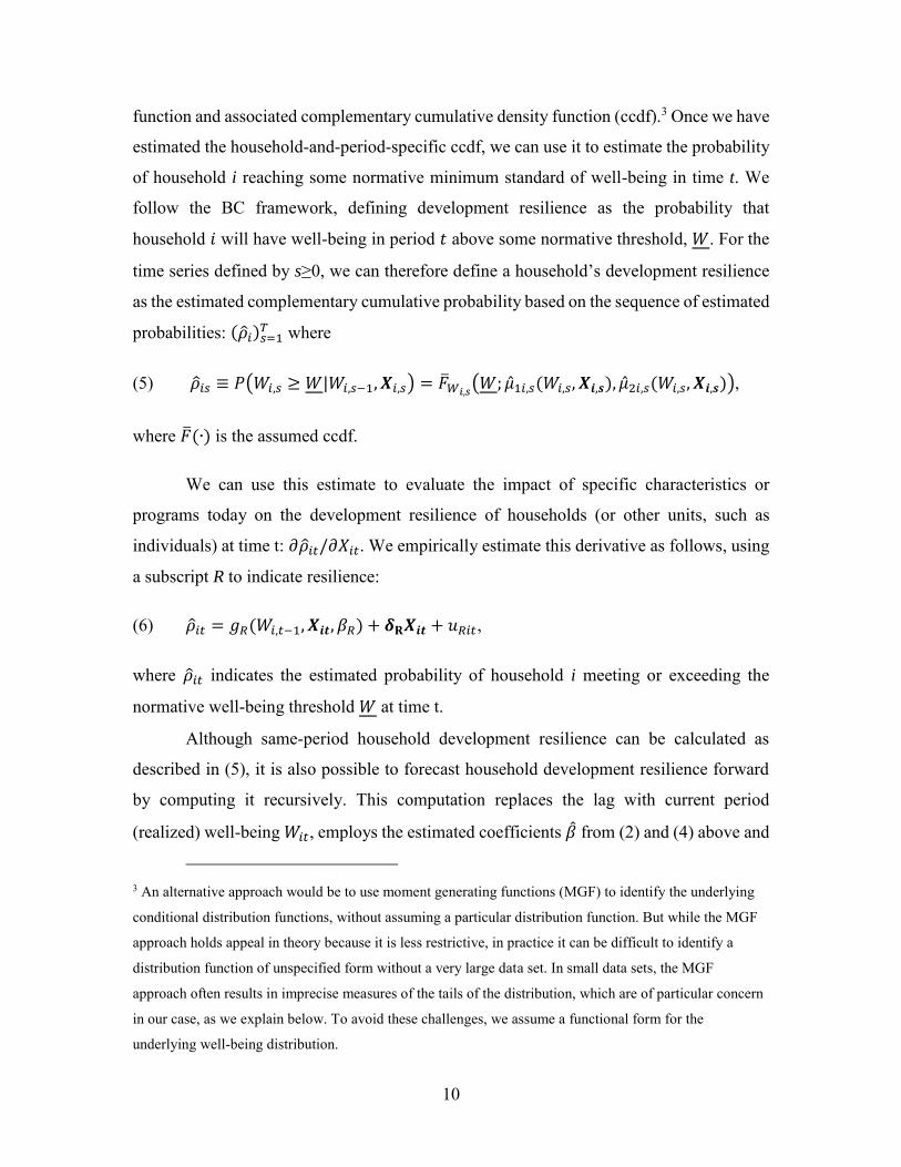
function and associated complementary cumulative density function (ccdf).3 Once we have

estimated the household-and-period-specific ccdf, we can use it to estimate the probability

of household i reaching some normative minimum standard of well-being in time t. We

follow the BC framework, defining development resilience as the probability that

household 𝑖 will have well-being in period 𝑡 above some normative threshold, 𝑊. For the

time series defined by s≥0, we can therefore define a household’s development resilience

as the estimated complementary cumulative probability based on the sequence of estimated

probabilities: (�̂�𝑖)𝑠=1𝑇 where

(5) �̂�𝑖𝑠 ≡ 𝑃(𝑊𝑖,𝑠 ≥ 𝑊|𝑊𝑖,𝑠−1, 𝑿𝑖,𝑠) = �̅�𝑊𝑖,𝑠(𝑊; �̂�1𝑖,𝑠(𝑊𝑖,𝑠, 𝑿𝒊,𝒔), �̂�2𝑖,𝑠(𝑊𝑖,𝑠, 𝑿𝒊,𝒔)),

where �̅�(∙) is the assumed ccdf.

We can use this estimate to evaluate the impact of specific characteristics or

programs today on the development resilience of households (or other units, such as

individuals) at time t: 𝜕�̂�𝑖𝑡/𝜕𝑋𝑖𝑡. We empirically estimate this derivative as follows, using

a subscript R to indicate resilience:

(6) �̂�𝑖𝑡 = 𝑔𝑅(𝑊𝑖,𝑡−1, 𝑿𝒊𝒕, 𝛽𝑅) + 𝜹𝐑𝑿𝒊𝒕 + 𝑢𝑅𝑖𝑡,

where �̂�𝑖𝑡 indicates the estimated probability of household i meeting or exceeding the

normative well-being threshold 𝑊 at time t.

Although same-period household development resilience can be calculated as

described in (5), it is also possible to forecast household development resilience forward

by computing it recursively. This computation replaces the lag with current period

(realized) well-being 𝑊𝑖𝑡, employs the estimated coefficients �̂� from (2) and (4) above and

3 An alternative approach would be to use moment generating functions (MGF) to identify the underlying

conditional distribution functions, without assuming a particular distribution function. But while the MGF

approach holds appeal in theory because it is less restrictive, in practice it can be difficult to identify a

distribution function of unspecified form without a very large data set. In small data sets, the MGF

approach often results in imprecise measures of the tails of the distribution, which are of particular concern

in our case, as we explain below. To avoid these challenges, we assume a functional form for the

underlying well-being distribution.

11

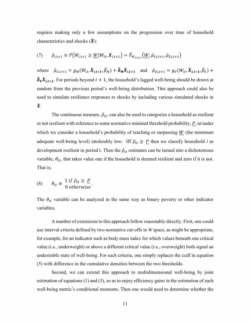
requires making only a few assumptions on the progression over time of household

characteristics and shocks (�̈�):

(7) �̂�𝑖,𝑡+1 ≡ 𝑃(𝑊𝑖,𝑡+1 ≥ 𝑊|𝑊𝑖𝑡, 𝑿𝑖,𝑡+1) = �̅�𝑊𝑖,𝑡+1(𝑊; �̂�1𝑖,𝑡+1, �̂�2𝑖,𝑡+1)

where �̂�1𝑖,𝑡+1 = 𝑔𝑀(𝑊𝑖𝑡, �̈�𝒊,𝒕+𝟏, �̂�𝑀) + �̂�𝐌�̈�𝒊,𝒕+𝟏 and �̂�2𝑖,𝑡+1 = 𝑔𝑉(𝑊𝑖𝑡, �̈�𝒊,𝒕+𝟏, �̂�𝑉) +

�̂�𝐕�̈�𝒊,𝒕+𝟏. For periods beyond 𝑡 + 1, the household’s lagged well-being should be drawn at

random from the previous period’s well-being distribution. This approach could also be

used to simulate resilience responses to shocks by including various simulated shocks in

�̈�.

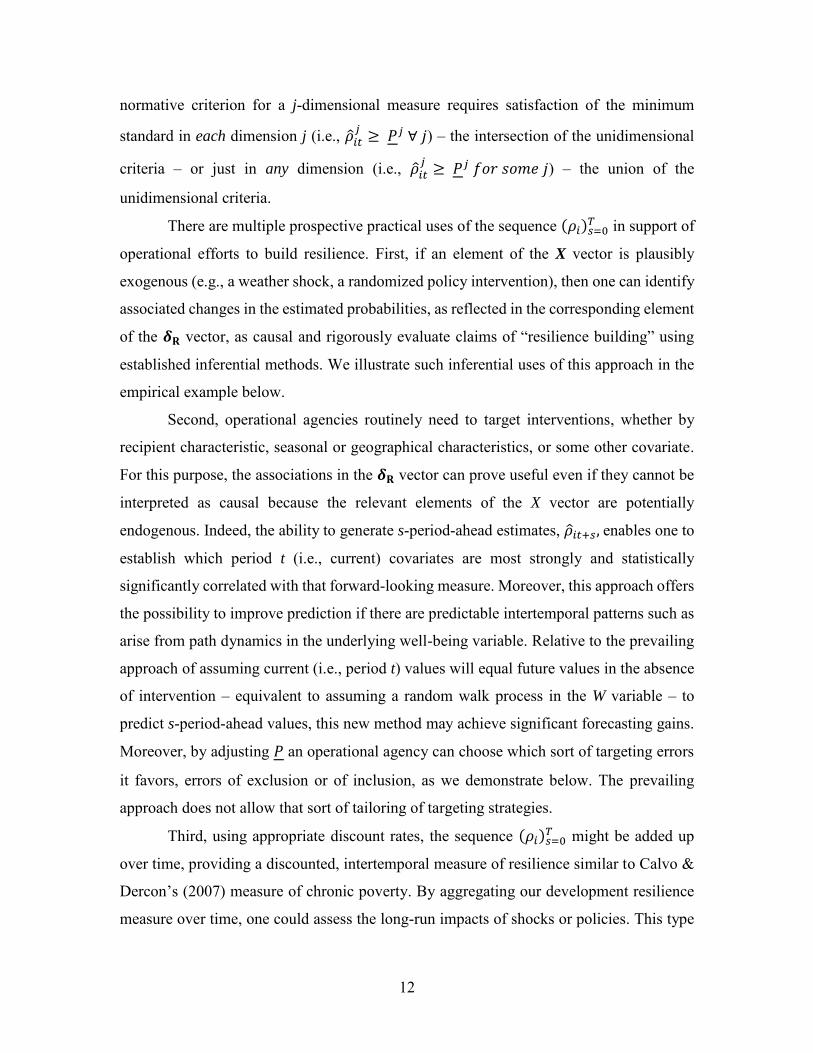
The continuous measure, �̂�𝑖𝑡, can also be used to categorize a household as resilient

or not resilient with reference to some normative minimal threshold probability, 𝑃, at/under

which we consider a household’s probability of reaching or surpassing 𝑊 (the minimum

adequate well-being level) intolerably low. Iff �̂�𝑖𝑡 ≥ 𝑃 then we classify household i as

development resilient in period t. Then the �̂�𝑖𝑡 estimates can be turned into a dichotomous

variable, 𝜃𝑖𝑡, that takes value one if the household is deemed resilient and zero if it is not.

That is,

(8) 𝜃𝑖𝑡 ≡ 1 𝑖𝑓 �̂�𝑖𝑡 ≥ 𝑃

0 𝑜𝑡ℎ𝑒𝑟𝑤𝑖𝑠𝑒.

The 𝜃𝑖𝑡 variable can be analyzed in the same way as binary poverty or other indicator

variables.

A number of extensions to this approach follow reasonably directly. First, one could

use interval criteria defined by two normative cut-offs in W space, as might be appropriate,

for example, for an indicator such as body mass index for which values beneath one critical

value (i.e., underweight) or above a different critical value (i.e., overweight) both signal an

undesirable state of well-being. For such criteria, one simply replaces the ccdf in equation

(5) with difference in the cumulative densities between the two thresholds.

Second, we can extend this approach to multidimensional well-being by joint

estimation of equations (1) and (3), so as to enjoy efficiency gains in the estimation of each

well-being metric’s conditional moments. Then one would need to determine whether the

12

normative criterion for a j-dimensional measure requires satisfaction of the minimum

standard in each dimension j (i.e., �̂�𝑖𝑡𝑗

≥ 𝑃𝑗 ∀ 𝑗) – the intersection of the unidimensional

criteria – or just in any dimension (i.e., �̂�𝑖𝑡𝑗

≥ 𝑃𝑗 𝑓𝑜𝑟 𝑠𝑜𝑚𝑒 𝑗) – the union of the

unidimensional criteria.

There are multiple prospective practical uses of the sequence (𝜌𝑖)𝑠=0𝑇 in support of

operational efforts to build resilience. First, if an element of the X vector is plausibly

exogenous (e.g., a weather shock, a randomized policy intervention), then one can identify

associated changes in the estimated probabilities, as reflected in the corresponding element

of the 𝜹𝐑 vector, as causal and rigorously evaluate claims of “resilience building” using

established inferential methods. We illustrate such inferential uses of this approach in the

empirical example below.

Second, operational agencies routinely need to target interventions, whether by

recipient characteristic, seasonal or geographical characteristics, or some other covariate.

For this purpose, the associations in the 𝜹𝐑 vector can prove useful even if they cannot be

interpreted as causal because the relevant elements of the X vector are potentially

endogenous. Indeed, the ability to generate s-period-ahead estimates, �̂�𝑖𝑡+𝑠, enables one to

establish which period t (i.e., current) covariates are most strongly and statistically

significantly correlated with that forward-looking measure. Moreover, this approach offers

the possibility to improve prediction if there are predictable intertemporal patterns such as

arise from path dynamics in the underlying well-being variable. Relative to the prevailing

approach of assuming current (i.e., period t) values will equal future values in the absence

of intervention – equivalent to assuming a random walk process in the W variable – to

predict s-period-ahead values, this new method may achieve significant forecasting gains.

Moreover, by adjusting 𝑃 an operational agency can choose which sort of targeting errors

it favors, errors of exclusion or of inclusion, as we demonstrate below. The prevailing

approach does not allow that sort of tailoring of targeting strategies.

Third, using appropriate discount rates, the sequence (𝜌𝑖)𝑠=0𝑇 might be added up

over time, providing a discounted, intertemporal measure of resilience similar to Calvo &

Dercon’s (2007) measure of chronic poverty. By aggregating our development resilience

measure over time, one could assess the long-run impacts of shocks or policies. This type

13

of intertemporal measure could also be used as a state variable in a dynamical system,

allowing for development resilience analysis in coupled human-natural systems.

Finally, these measures can be used to identify development resilience indicators at

more aggregated scales of analysis. We now turn to this task of development resilience

aggregation, to follow Sen’s (1979) term, which represents a straightforward adaptation of

today’s workhorse FGT class of decomposable poverty measures to the individual

measures just introduced.

III. DEVELOPMENT RESILIENCE AGGREGATION

Sen describes the aggregation process as “some method of combining deprivations of

different people into some over-all indicator” (Sen 1979, p.288). While the approach

discussed in Section II allows us to identify the level of development resilience of a specific

unit (such as an individual or household), we would also like to summarize the

development resilience of the micro units into one overall sub-population or population-

level resilience measure, the aggregate resilience index 𝑅.

Even before Foster, Greer, & Thorbecke (1984) proposed a class of decomposable

poverty measures, now known simply as the FGT poverty measures, certain desirable

attributes for poverty measures had been discussed in the literature. Sen (1976) highlights

some of the shortcomings of the headcount ratio, such as its violation of the monotonicity

and transfer axioms.4 Sen proposed a poverty measure that meets additional desirable

characteristics he sets out, including “relative equity,”5 and conveniently lies between 0

and 1. Sen also argues that a poverty measure would ideally combine “considerations of

absolute and relative deprivation even after a set of minimum needs and a poverty line have

been fixed” (Sen 1979, p.293).

4 The Monotonicity Axiom states: “Given other things, a reduction in income of a person below the poverty

line must increase the poverty measure” (Sen 1976, p.219). The Transfer Axiom states: “Given other

things, a pure transfer of income from a person below the poverty line to anyone who is richer must

increase the poverty measure” (Sen 1976, p.219). 5 Relative Equity requires “that if person i is accepted to be worse off than person j in a given income

configuration y, then the weight vi on the income short-fall gi of the worse-off person i should be greater

than the weight vj on the income short-fall gj” (Sen 1976, p. 221).

14

Another desirable feature of any aggregate measure is the ability to attribute shares

of the overall development resilience indicator to various subgroups. The population-

weighted sum of the subgroup measures would therefore equal the measure for the whole

group. While the measure proposed by Sen is not decomposable in this way, FGT (1984)

proposed an entire class of decomposable poverty measures and illustrated how the

measures meet Sen’s (1976, 1979) various axioms. The FGT (1984) poverty measures

serve as a logical jumping off point in the search for an additive development resilience

measure that meets Sen’s axiomatic requirements.

As a quick refresher, for a vector of household incomes, 𝑦, ordered from lowest to

highest, poverty line 𝑧 > 0, and income gap 𝑔𝑖 ≡ 𝑧 − 𝑦𝑖, there are 𝑞 households in a

population of size 𝑛 at or below the poverty line. FGT (1984) proposed the measure

𝑃𝛼(𝑦; 𝑧) =1

𝑛∑ (

𝑔𝑖

𝑧)

𝛼𝑞𝑖=1 , which meets the Sen criteria and is additively decomposable with

population share weights for different subpopulations of 𝑛. When 𝛼 = 0 this is equivalent

to the headcount ratio, when 𝛼 = 1 this is equivalent to the poverty gap index, and when

𝛼 = 2 it is the poverty severity index, also known as the squared poverty gap index

(Haughton & Khandker 2009). By weighting each household’s poverty gap by its

proportion of the gap, the squared index not only considers absolute deprivation (by

focusing on those below the poverty line 𝑧), but also relative deprivation (placing higher

weights on those further below the poverty line).

Following FGT (1984), we propose a decomposable development resilience

indicator that aggregates the individual- or household-specific development resilience

probabilities, �̂�𝑖𝑡, developed in Section II across the population into a single economy-wide

measure that is also decomposable to describe distinct sub-populations. Just as with the

FGT family of measures from which the development resilience index is adapted, this

measure meets the monotonicity, transfer, and relative equity axioms proposed by Sen in

addition to being additively decomposable among groups. A demonstration of how this

measure satisfies the various axioms set forth by Sen (1976, 1979) and FGT can be found

in Appendix A.

Assume a normative resilience probability threshold of 𝑃 (1 ≥ 𝑃 ≥ 0), as discussed

above, at/under which we consider a household’s probability of reaching or surpassing 𝑊

15

(the normative threshold well-being level discussed in Section II) to be intolerably low.

The resilience analyst must therefore select two normative thresholds, 𝑊 and 𝑃, which

may be context specific. Suppressing time period subscripts for now, we generate a vector

𝝆 of household development resilience measures in time period 𝑡 + 𝑠 ordered from lowest

to highest values, 𝝆 = (�̂�1, �̂�2, �̂�3, … , �̂�𝑛; 𝑊) for a total number of 𝑛 households. With this

information we can count the number of non-resilient households, 𝑞, for which the

household resilience probability falls at or below the resilience probability threshold 𝑞 =

𝑞(𝝆; 𝑃), as well as the resilience shortfall (measured in probabilities) for those households

𝑔𝑖 = 𝑃 − �̂�𝑖. In the index, this gap is then weighted by 𝛼, a distribution sensitivity

parameter that FGT refer to as the measure of poverty aversion.

The sum of the weighted gaps is subtracted from one to ensure that larger numbers

signify increased resilience. The decomposable resilience index is therefore defined for

period 𝑡 + 𝑠 as

(9) 𝑅𝛼,𝑡+𝑠(𝝆𝒕+𝒔; 𝑊, 𝑃) ≡ 1 − [1

𝑛∑ (

𝑔𝑖,𝑡+𝑠

𝑃)

𝛼𝑞𝑡+𝑠𝑖=1 ],

and the sequence of resilience indices, (𝑅𝛼,𝑡+𝑠)𝑠=0

𝑇, would represent aggregate resilience

over time to horizon period T. The measure necessarily lies on the closed interval [0,1],

with 𝑅 = 0 if each household in the population has a development resilience probability

estimate �̂�𝑖 < 𝑃 ∀ 𝑖 ∈ 𝑛, and 𝑅 = 1 if �̂�𝑖 ≥ 𝑃 ∀ 𝑖 ∈ 𝑛, implying 𝑞 = 0. This approach

allows us to calculate the population share deemed resilient (i.e., development resilience

headcount ratio) when 𝛼 = 0 (𝐻𝑅 ≡𝑛−𝑞

𝑛), mean development resilience of non-resilient

household (�̅�𝑞 =∑ �̂�𝑖

𝑞𝑖=1

𝑞), as well as the resilience-gap ratio (𝐺 ≡ ∑

𝑔𝑖

𝑞𝑃

𝑞𝑖=1 ). It is therefore

well suited for situations in which resilience indices would be useful for targeting or for

policy/project evaluation. Given that the poor are the least economically resilient by the

BC definition, and for any measure based on a poverty-related welfare indicator, 𝑊, the

measure is inherently pro-poor.

16

IV. AN EMPIRICAL EXAMPLE

To illustrate this method, we now employ the development resilience estimation and

aggregation techniques discussed above using household data from northern Kenya. The

Horn of Africa is a particularly relevant context for the implementation of a resilience

measure, as the 2011 drought in the region was one of the main drivers of governmental

and non-governmental organization interest in resilience. In northern Kenya, pastoralist

communities rely heavily on livestock to generate most or all of their income. Few other

livelihoods are viable given agroecological conditions and meager modern infrastructure

(McPeak, Little, & Doss 2012). These households are incredibly vulnerable to weather

shocks, such as drought, which can decimate herds. Prior research in the area has

established, in multiple data sets, that multiple equilibrium poverty traps exist in livestock

holdings, and that drought risk is a key driver of households’ collapse into persistent

poverty (Lybbert et al. 2004, Barrett et al. 2006, Santos and Barrett 2011). To help pastoral

and agro-pastoral populations manage drought-related livestock mortality, an index-based

livestock insurance (IBLI) product was piloted in northern Kenya beginning in January

2010 (Chantarat et al. 2013).

The data used in this example were collected by a consortium led by the

International Livestock Research Institute (ILRI), in collaboration with private insurance

providers, using a multi-year impact evaluation strategy (ILRI 2013). The household

surveys gathered information from 924 randomly selected households in Marsabit County,

including general demographic variables as well as data on livestock holdings and

production, risk and insurance, livelihood activities, expenditure and consumption, assets,

and savings and credit. Five rounds6 of the annual survey have been administered each

October-November, beginning in 2009.

The IBLI product uses normalized difference vegetation index (NDVI) estimates

derived from satellite data to predict livestock mortality. When predicted livestock

mortality due to drought, as reflected in low NDVI values, reaches catastrophic levels

6 Five rounds of the data are available and used in this analysis. Since we use lagged variables, the first

round of the data is not used (with the exception of the lagged well-being (livestock) data). A sixth round of

data has recently been collected but has not yet been included in this analysis.

17

(contractually defined as 15% estimated area average loss), the insurance policy pays out.

During the five rounds of data, a catastrophic drought occurred once, between rounds two

and three.

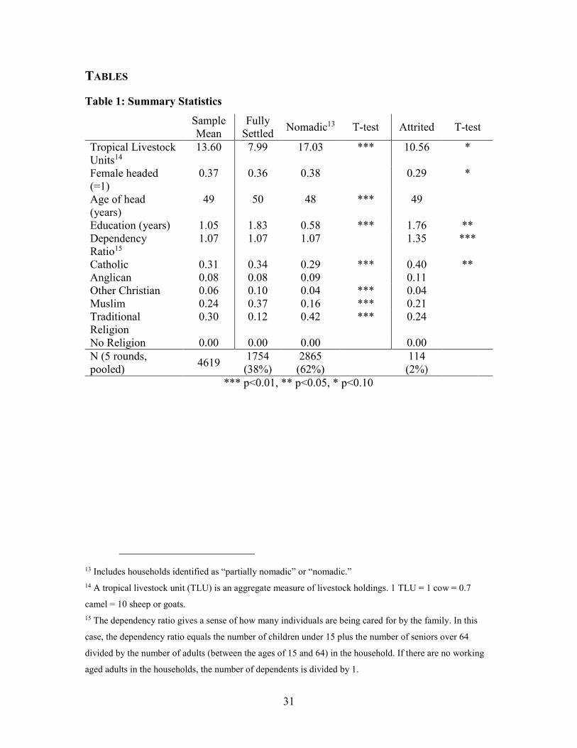
Table 1 presents summary statistics. We distinguish between fully settled

households that never relocated and those partially or fully nomadic households that

relocated, at least seasonally, as they migrated their herds over longer distances in search

of forage and water. Nearly two-thirds of the sample is (at least partly) nomadic.

Sedentarized households have significantly fewer livestock holdings, greater (albeit still

limited) educational attainment, and are much more likely to practice Islam. The pooled

sample attrition rate is approximately 2%. Of these, some households are absent for a given

round and then reappear in subsequent rounds.7 Attrited households are somewhat more

likely to be Catholic and have slightly fewer livestock holdings than the mean household.

The dependency ratio is higher for attrited households, which may partially explain why

no one was available to respond to the survey during a given round.

Development Resilience Estimation

Because most survey households hold a large share of their wealth in livestock and

depend heavily on livestock to generate income, livestock holdings offer a logical (and

commonplace) measure of well-being in pastoralist settings. The primary household well-

being variable of interest, therefore, is household aggregate livestock holdings, expressed

in tropical livestock units (1 TLU = 1 cow = 0.7 camel = 10 sheep or goats) in each survey

round.

TLU holdings are estimated via maximum likelihood, per equation (1), as a

polynomial function of lagged well-being (i.e., TLU from the previous period), a dummy

variable indicating a serious drought (i.e., area average predicted losses ≥ 15% per the IBLI

index), the sex of the household head, the age and squared age of the household head to

7 Due to the lagged variable in our estimation, the household that is not contacted in one round is actually

absent from the estimation for that round and the next, and the household is counted as attrited in both

rounds.

18

account for life cycle effects, the number of years of education for the household head, the

household dependency ratio, and controls for religious affiliation and nomadic status:

(10) 𝑊𝑖𝑡 = ∑ �̂�𝑀𝛾𝑊𝑖,𝑡−1𝛾4

𝛾=1 + 𝜹𝐌𝑿𝒊𝒕 + 𝑢𝑀𝑖𝑡.

As mentioned above, a third order polynomial in lagged TLU holdings is the most

parsimonious that can accommodate the S-shaped herd dynamics found in prior studies in

the region (Barrett et al. 2006). For this empirical example, tests of the various polynomial

specifications can be found in Table B1 in Appendix B. In this case, the Akaike information

criterion (AIC) values are decreasing in polynomial order, suggesting a higher order

specification would be preferred. However, the coefficient estimates on the higher order

lagged well-being terms are effectively zero. A t-test on the equality of means between the

predicted values of the higher-order specifications finds statistically insignificant

differences for everything above and including the fourth order. Therefore, the fourth order

specification is preferred in this case.

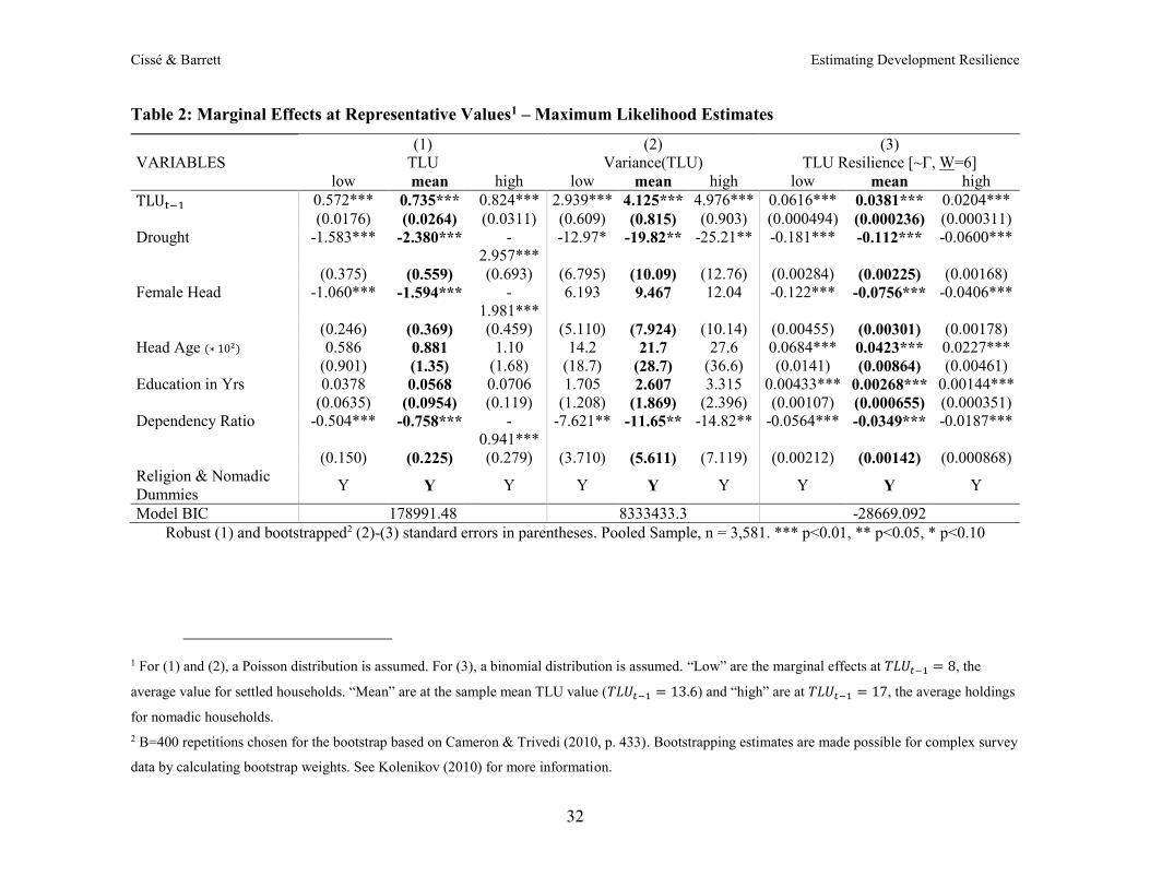
Given that physical livestock holdings must be non-negative, the dependent

variable is assumed to be distributed Poisson. The generalized linear model (GLM) log link

regression is fit using maximum likelihood and Table 2 column (1) displays the marginal

effects estimates for mean TLU well-being, as well as for low and high values of lagged

TLU holdings. Consistent with prior studies of east African livestock wealth dynamics,

herd dynamics are statistically significantly nonlinear, as evidenced by the difference

between the marginal effect at a low value of past period TLU holdings and at a high value.

Marginal effects at the mean of all covariates are presented in the bolded, middle column.

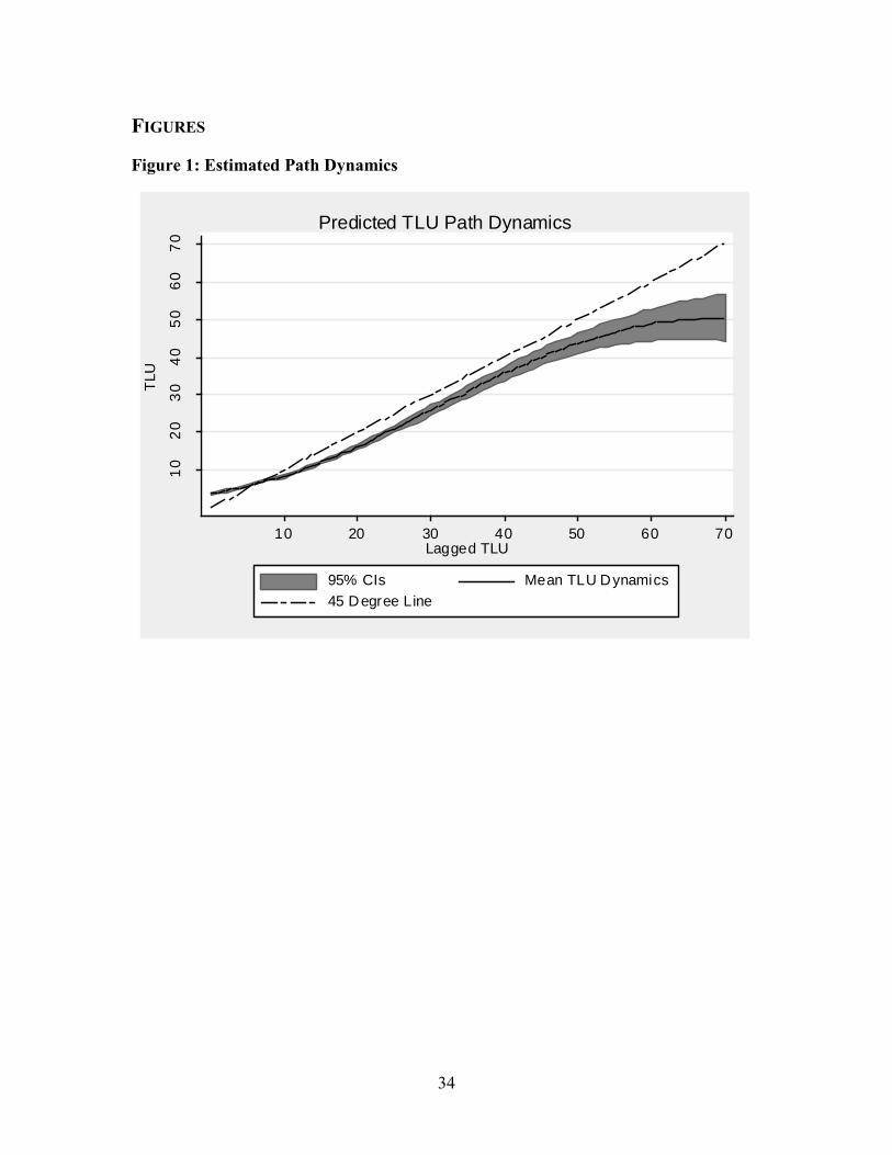
Figure 1 displays estimated herd dynamics based on the marginal effects calculated in

Table 2 column (1), valuing other covariates at sample means. Although there is evidence

of S-shaped TLU dynamics, unlike prior empirical studies of herd dynamics using earlier

datasets from the region, there is no evidence of multiple TLU equilibria, although this

could simply reflect limited recovery time from the catastrophic 2011 drought in a short

sample. Rather, this parametric estimation suggests a unique stable dynamic equilibrium

at approximately 6 TLU. The coefficient estimate on drought is, as expected, strongly and

statistically significantly negative, with an estimated average 2.4 TLU loss in a major

drought associated with a one unit increase in lagged TLU, representing an 18% average

19

loss relative to sample mean livestock holdings. For households with low past period

livestock holdings, the marginal effect of drought—while still statistically significantly

negative—is smaller in absolute terms, but actually represents a slightly larger proportion

of their livestock holdings (20%). Holding previous period herd size constant, female

headed households have statistically significantly smaller herds than male headed

households, as do households with more dependents. The coefficient estimates on the age

of the household head and on his/her education are not statistically significantly different

from zero.

Following equation (3), we capture the residuals from the mean well-being equation

just reported, square them, and use these values to estimate the conditional variance

equation, also via maximum likelihood,8

(11) �̂�𝑖𝑡2 = ∑ �̂�𝑉𝛾𝑊𝑖,𝑡−1

𝛾4𝛾=1 + 𝜹𝐕𝑿𝒊𝒕 + 𝑢𝑉𝑖𝑡.

The estimates for the TLU variance equation can be found in column (2) of Table

2, again displayed at various values of lagged TLU holdings. There is statistically

significant nonlinear autoregressive conditional heteroscedasticity as reflected in the

coefficient estimates of lagged herd size; the marginal effect of lagged TLU on conditional

variance is 60% larger for households with higher previous period TLU holdings. Drought

and the dependency ratio are also statistically significantly (and negatively) related to the

conditional variance of herd size, while the other covariates are not. This indicates that

there is less variance in times of drought, indicating that drought suppresses variation while

it also lowers mean well-being.

Using the estimates from columns (1) and (2) in Table 2, we can estimate each

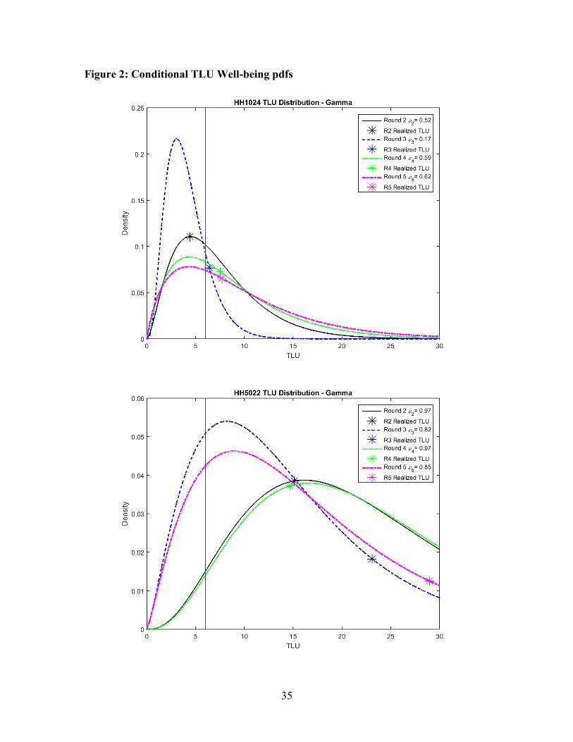
household’s TLU probability density function (pdf) for each period. Figure 2 shows how

the estimated TLU pdfs—in this case based on the gamma distribution9—vary, both over

time and across households: Household 1024 is a female-headed, fully settled household

8 As with the mean equation, the dependent variable (variance) must be non-negative. As such, once again

we assume the dependent variable is distributed Poisson and fit the GLM log link regression using

maximum likelihood.

9 Distribution parameters for the gamma distribution are: 𝑊𝑡|𝑊𝑡−1~Γ(𝜇2𝑡

𝜇1𝑡,

𝜇1𝑡2

𝜇2𝑡), based on Bury (1999).

20

fairly typical of that sub-group in terms of livestock holdings, education, and age, while

Household 5022 is a male-headed, nomadic household with TLU holdings near that sub-

group’s mean. The former household is markedly poorer in terms of livestock than the

latter, with lower expected TLU levels across all periods. Although the round following

the drought shock (Round 3) sees a marked decrease in resilience for the female headed

household, the household well-being improves markedly in the two post shock years, as

reflected in leftward and rightward shifts of the pdfs, respectively. In fact, the household is

able to achieve higher resilience in Rounds 4 and 5 than in the initial period. Although

household 5022 is relatively well-off in terms of TLU holdings, it is also dramatically

affected by the drought shock; household well-being falls to its lowest levels during Round

3. The household is able to fully recover in Round 4 before being impacted by an

idiosyncratic shock in the final round.

After calculating the household-specific pdfs, the next step is to estimate each

household’s probability of achieving the normative minimum well-being (𝑊) in each

period. We set the threshold level at 6 TLU (𝑊 = 6), which is the critical livestock

threshold previously identified in the literature for this region of northern Kenya (Barrett

et al. 2006). This threshold is represented in Figure 2 by the vertical line. The household-

specific development resilience estimate for each period, �̂�𝑖𝑡, is simply household i’s

complementary cumulative probability beyond the threshold value, 𝑊, in period t, per

equation (5). Each household-period-specific resilience score therefore lies in the interval

[0,1].

Following equation (6), we can regress these household-and-period-specific

resilience scores on the same regressors used in the mean and variance equations, as

follows:

(12) �̂�𝑖𝑡 = ∑ �̂�𝑅𝛾𝑊𝑖,𝑡−1𝛾4

𝛾=1 + 𝜹𝐑𝑿𝒊𝒕 + 𝑢𝑅𝑖𝑡.

We do this estimation because the resilience score is a nonlinear function of the (linear)

estimates of the conditional mean and conditional variance. The fractional response

21

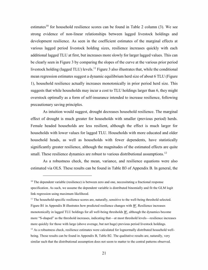
estimates10 for household resilience scores can be found in Table 2 column (3). We see

strong evidence of non-linear relationships between lagged livestock holdings and

development resilience. As seen in the coefficient estimates of the marginal effects at

various lagged period livestock holding sizes, resilience increases quickly with each

additional lagged TLU at first, but increases more slowly for larger lagged values. This can

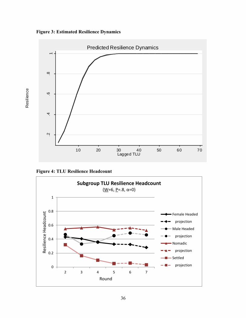
be clearly seen in Figure 3 by comparing the slopes of the curve at the various prior period

livestock holding (lagged TLU) levels.11 Figure 3 also illustrates that, while the conditional

mean regression estimates suggest a dynamic equilibrium herd size of about 6 TLU (Figure

1), household resilience actually increases monotonically in prior period herd size. This

suggests that while households may incur a cost to TLU holdings larger than 6, they might

overstock optimally as a form of self-insurance intended to increase resilience, following

precautionary saving principles.

As intuition would suggest, drought decreases household resilience. The marginal

effect of drought is much greater for households with smaller (previous period) herds.

Female headed households are less resilient, although the effect is much larger for

households with lower values for lagged TLU. Households with more educated and older

household heads, as well as households with fewer dependents, have statistically

significantly greater resilience, although the magnitudes of the estimated effects are quite

small. These resilience dynamics are robust to various distributional assumptions.12

As a robustness check, the mean, variance, and resilience equations were also

estimated via OLS. These results can be found in Table B3 of Appendix B. In general, the

10 The dependent variable (resilience) is between zero and one, necessitating a fractional response

specification. As such, we assume the dependent variable is distributed binomially and fit the GLM logit

link regression using maximum likelihood. 11 The household-specific resilience scores are, naturally, sensitive to the well-being threshold selected.

Figure B1 in Appendix B illustrates how predicted resilience changes with 𝑊. Resilience increases

monotonically in lagged TLU holdings for all well-being thresholds 𝑊, although the dynamics become

more “S-shaped” as the threshold increases, indicating that—at most threshold levels—resilience increases

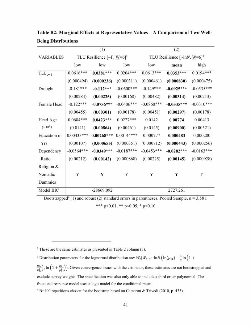
more quickly for those with large (above average, but not huge) previous period livestock holdings. 12 As a robustness check, resilience estimates were calculated for lognormally distributed household well-

being. Those results can be found in Appendix B, Table B2. The qualitative results are, naturally, very

similar such that the distributional assumption does not seem to matter to the central patterns observed.

22

two methods confirm the importance of path dynamics (in significance and magnitude) for

both the variance and resilience equations, as well as the negative impact of drought on

TLU well-being. The signs are not consistent, however, between the different

specifications. Surprisingly, the estimated coefficient on education in the OLS resilience

equation is negative, although the magnitude is negligible.

Development Resilience Aggregation

In order to generate aggregate development resilience measures for a population

from the set of household-specific estimates, we must first select a minimum probability

threshold, 𝑃, above which a household is deemed resilient and below which it is considered

not resilient. This second normative threshold is necessary because development resilience

is a probabilistic measure, unlike directly observable indicators such as expenditures,

income or livestock holdings. We set 𝑃 = 0.80, meaning that we only consider household

i resilient if it has at least an 80% probability of reaching the well-being threshold (i.e.,

�̂�𝑖𝑡 ≡ Pr(𝑊𝑖𝑡 ≥ 𝑊 = 6|𝑊𝑖,𝑡−1, 𝑿𝒊𝒕) ≥ 0.80). Setting the distribution sensitivity

parameter, 𝛼 = 0, so as to generate a headcount estimate of the population share who are

not resilient, for the entire sample, pooled across periods, we estimate

(13) 𝑅0(𝝆𝑻𝑳𝑼; 6, 0.8) ≡ 1 − [1

𝑛∑ (

𝑔𝑖

0.8)

0𝑞𝑖=1 ] = 0.394,

meaning that about forty percent of households in the pooled sample are development

resilient by this measure.

One of the appealing features of FGT-style measures like R is their

decomposability. The sample population can be broken down into various subgroups by

characteristics such as sex or education of the household head, nomadic status, geographic

area, etc. Another benefit of this new development resilience estimation approach is that

the built-in path dynamics facilitate development resilience forecasting, projecting how

resilience will evolve in future periods, given current and recently observed values. This

allows us to forecast development resilience estimates for each household, and therefore

the aggregate subgroup resilience measures, as well, under different scenarios. We can

23

simulate how, for example, development resilience will develop in the absence (or

presence) of another drought shock.

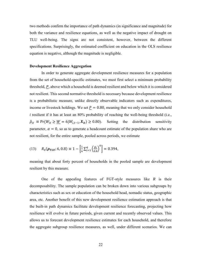
Given the perceived vulnerability of female headed and settled households in this

region, we calculate the headcount resilience index by sex and nomadic status per equation

(9) and project the measures out two years into the future based on a few reasonable

assumptions about the evolution of covariates, such as that the education of the household

head remains unchanged while his or her age increases by one year each year, as described

in equation (7). The dashed lines from periods 5 to 7 in Figure 4 show how development

resilience is predicted to evolve over the two years following the fifth survey round if

households in Marsabit do not suffer another catastrophic drought.

We calculate the sex-specific headcount measure for each round so as to observe

the evolution of development resilience over the course of a drought cycle. Although

headcount resilience is quite similar for male and female headed households in Round 2,

female headed households do not appear to be as substantially impacted by the drought as

male headed households at first. Although their initial headcount resilience drop is less

substantial, female headed households appear unable to recover. The headcount resilience

score continues to decline over the survey period and is projected to drop even further.

Male headed households, on the other hand, see a sharp drop in their headcount resilience

post-drought. Importantly, these households recover most of their lost resilience within

three years of the drought and were forecast to maintain that level of resilience in

subsequent years.

Given longstanding observations in the region that nomadic households are better-

off and seemingly more resilient to drought due to their mobility (Barrett et al. 2006, Little

et al. 2008), we also explore how this development resilience measure varies by nomadic

status. As depicted in Figure 4, nomadic households are indeed consistently more resilient

than are settled households. The difference in resilience among households also appears

far more pronounced in the mobility/nomadism dimension than based on gender of the

household head. Consistent with the aforementioned observations, the headcount resilience

score for nomadic households is seemingly unaffected by the drought, while settled

households see a sharp initial drop and, as with female headed households, seem unable to

recover in subsequent or project rounds.

24

Targeting

The resilience differences based on nomadic status suggest a targetable

characteristic for interventions aimed at boosting the resilience of vulnerable households.

This method and the estimates it generates can help to identify the key populations in need

of assistance in order to boost and/or buffer their resilience or for targeting specific types

of interventions estimated to have especially pronounced expected effects on household

resilience. Because good targeting necessarily involves forecasting where a household

would be in the absence of an intervention, the (potentially nonlinear) conditional path

dynamics built into this method of development resilience estimation offer a significant

opportunity to improve targeting. Conventional methods use the most recent observation

of a household as the best estimate of the future state in the absence of an intervention. But

that implicitly imposes a strong assumption of a random walk stochastic process. In the

empirical example above, we can reject the null hypothesis of a random walk, suggesting

that our method might enhance targeting accuracy.

The strength of the development resilience approach is that it allows us to look at

the probability of maintaining well-being over time, and leverage the inter-temporal

variation captured by the panel dataset to predict future outcomes. In order to assess the

targeting accuracy of this approach vis-à-vis conventional approaches, we could compare

targeting accuracy rates (both correctly targeted and correctly not targeted), Type I errors

(errors of inclusion, i.e., those targeted who nonetheless exceeded the threshold) and Type

II errors (i.e., errors of exclusion, those not targeted who nonetheless fell below the

threshold), for different probability thresholds (𝑃) for a standard targeting approach (based

on the most recently observed value) and a resilience-based targeting approach, as

described in Upton, Cissé, and Barrett (2016).

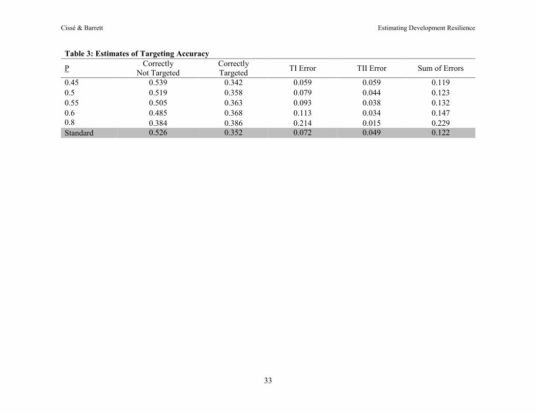
Table 3 presents the estimates of targeting accuracy for an intervention in Round 5,

based on the development resilience approach described above (using data from Rounds 1-

4) and compares it to a standard targeting regime based only on realized TLU holdings in

Round 4. While no probability threshold 𝑃 consistently outperforms the standard approach

on all measures, a probability threshold can be selected that outperforms the standard

model for each of the various measures. That is, while the standard approach does not allow

implementers to choose between inclusion and exclusion errors in targeting, the

25

development resilience approach explicitly allows policymakers to choose between

leakage and over-coverage depending on priorities and resource constraints. Importantly,

resilience-based targeting outperforms the standard approach on the measure of interest

given decision-makers’ priorities.

V. CONCLUSIONS AND POLICY IMPLICATIONS

Given the disastrous impacts of increasingly frequent natural disasters, cyclical food

assistance needs, and limited humanitarian budgets, international development and

humanitarian agencies have recently begun to focus heavily on resilience. The empirical

development resilience approach developed here provides an econometric strategy for

understanding potentially nonlinear well-being dynamics in shock-prone contexts,

bringing together relevant concepts from the poverty traps, risk, vulnerability, and poverty

measurement literatures.

As the empirical example demonstrates, it is important to understand mean well-

being dynamics in order to design appropriate interventions. As Barrett & Carter (2013)

explain, well-targeted transfers to individuals just below a poverty trap threshold may help

them escape poverty, but the same transfers would have negligible impacts in contexts such

as the one discussed in this paper, with unique, low-level well-being equilibria. But

understanding the mean well-being dynamics is not sufficient, as ignoring high-order

moments obscures the impact of risk and self-insurance on well-being. In Northern Kenya,

households (particularly nomadic households) acquire herds much larger than dynamic

equilibrium levels, and at considerable cost. The development resilience approach offers

insight into this seemingly costly and long-run futile behavior, by uncovering the

correlation between large herd sizes and higher probabilities of future well-being.

While the benefits of a rigorous empirical analysis of development resilience are

clear, the data are currently not available to allow this type of analysis at scale. We support

calls for a multi-country system of sentinel sites collecting high-quality, high-frequency

data over long periods of time, particularly in the most disaster-prone parts of the world

(Barrett & Headey 2014, Headey & Barrett 2015). Yet the absence of such data should not

prevent methodological contributions, but rather guide developments in data collection and

management systems. We hope that the methods introduced in this paper provide some

26

direction and impetus for increased data collection while also providing a template for

resilience estimation in contexts with adequate data availability, which are growing

increasingly common.

REFERENCES

Adato, Michelle, Michael R. Carter, and Julian May. 2006. “Exploring Poverty Traps and

Social Exclusion in South Africa Using Qualitative and Quantitative Data.” The

Journal of Development Studies 42(2): 226-47.

Alfani, Federica, Andrew Dabalen, Peter Fisker, and Vasco Molini. 2015. “Can We

Measure Resilience? A Proposed Method and Evidence from Countries in the

Sahel.” Policy Research Working Paper #7170, World Bank Group – Poverty

Global Practice Group.

Alinovi, Luca, Erdgin Mane, and Donato Romano. 2010. “Measuring Household

Resilience to Food Insecurity: Application to Palestinian Households.” In

Agricultural Survey Methods, edited by Roberto Benedetti, Marco Bee, Giuseppe

Espa, and Federica Piersimoni. Chichester, U.K.: John Wiley & Sons.

Antle, John M. 1983. “Testing the Stochastic Structure of Production: A Flexible Moment-

Based Approach.” Journal of Business & Economic Statistics 1(3): 192-201.

Antman, Francisca and David McKenzie. 2007.” Poverty traps and nonlinear income

dynamics with measurement error and individual heterogeneity.” Journal of

Development Studies 43(6): 1057-83.

Barrett, Christopher B. and Michael R. Carter. 2013. “The Economics of Poverty Traps

and Persistent Poverty: Empirical and Policy Implications.” Journal of

Development Studies 49(7): 976-990.

Barrett, Christopher B. and Mark A. Constas. 2014. “Toward a Theory of Resilience for

International Development Applications.” Proceedings of the National Academy of

Sciences 40(111): 14625–14630.

Barrett, Christopher B. and Derek Headey. 2014. “Measuring Resilience in a Volatile

World: A Proposal for a Multicountry System of Sentinel Sites.” Paper prepared

for the 2020 Vision Initiative. Washington: International Food Policy Research

Institute.

27

Barrett, Christopher B., Paswel Phiri Marenya, John McPeak, Bart Minten, Festus Murithi,

Willis Oluoch-Kosura, Frank Place, Jean Claude Randrianarisoa, Jhon

Rasambainarivo, and Justine Wangila. 2006. "Welfare Dynamics in Rural Kenya

and Madagascar." Journal of Development Studies 42(2): 248-77.

Béné, Christophe, Andrew Newsham, Mark Davies, Martina Ulrichs, and Rachel Godfrey-

Wood. 2014. “Review Article: Resilience, Poverty and Development.” Journal of

International Development 26: 598-623.

Bury, Karl. 1999. Statistical Distributions in Engineering. Cambridge, UK: Cambridge

University Press.

Calvo, Cesar and Stefan Dercon. 2007. “Chronic poverty and all that: the measurement of

poverty over time.” CPRC Working Paper 89, Chronic Poverty Research Centre.

Cameron, A. Colin and Pravin K. Trivedi. 2010. Microeconomics Using Stata: Revised

Edition. College Station, TX: Stata Press.

Cannon, Terry and Detkef Müller-Mahn. 2010. “Vulnerability, Resilience and

Development Discourses in the Context of Climate Change.” Natural Hazards

55(3): 621-635.

Carter, Michael R. and Christopher B. Barrett. 2006. “The economics of poverty traps and

persistent poverty: An asset-based approach.” Journal of Development Studies

42(2): 178-199.

Carter, Michael R. and Julian May. 2001. “One Kind of Freedom: Poverty Dynamics in

Post-apartheid South Africa.” World Development 29(12): 1987-2006.

Chantarat, Sommarat, Andrew G. Mude, Christopher B. Barrett, and Michael R. Carteret.

2013. “Designing Index-Based Livestock Insurance for Managing Asset Risk in

Northern Kenya.” Journal of Risk and Insurance 80: 205–237. doi: 10.1111/j.1539-

6975.2012.01463.x

Chaudhuri, Shubham, Jyotsna Jalan, and Asep Suryahadi. 2002. “Assessing Household

Vulnerability to Poverty from Cross-sectional Data: a Methodology and Estimates

for Indonesia.” Discussion Paper Series No. 0102-52, Department of Economics,

Columbia University, New York.

28

Christiaensen, Luc J. and Richard N. Boisvert. 2000. “On Measuring Household Food

Vulnerability: Case Evidence from Northern Mali.” Cornell University Department

of Economics Working Paper. WP 2000-05.

Constas, Mark A., Timothy R. Frankenberger, and John Hoddinott. 2014. “Resilience

Measurement Principles: Toward an Agenda for Measurement Design.” Food

Security Information Network, Resilience Measurement Technical Working

Group, Technical Series No. 1.

Davoudi, Simin. 2012. “Resilience: A Bridging Concept or a Dead End?” Planning Theory

& Practice 13(2): 299–333.

Folke, Carl. 2006. “Resilience: The Emergence of a Perspective for Social-Ecological

Systems Analyses.” Global Environmental Change 16 (2006): 253-67.

Foster, James, Joel Greer, and Erik Thorbecke. 1984. “A Class of Decomposable Poverty

Measures.” Econometrica 52(3): 761-66.

Haughton, Jonathan and Shahidur R. Khandker. 2009. Handbook on Poverty and

Inequality. Washington, DC: The World Bank.

Headey, Derek and Christopher B. Barrett. 2015. “Measuring Development Resilience in

the World’s Poorest Countries.” Proceedings of the National Academy of Sciences

112(37): 11423-5.

Hoddinott, John and Agnes Quisumbing. 2003. “Methods for Microeconometric Risk and

Vulnerability Assessments.” Social Protection Discussion Paper No 0324, Human

Development Network, the World Bank.

International Livestock Research Institute. 2013. “Index Based Livestock Insurance for

Northern Kenya’s Arid and Semi-Arid Lands: The Marsabit Project - Codebook for

IBLI Evaluation Survey (Round 1, Round 2, Round 3 and Round 4 Surveys).”

http://data.ilri.org/portal/dataset/ibli-marsabit-r1

Just, Richard E. and Rulon D. Pope. 1979. “Production Function Estimation and Related

Risk Considerations.” American Journal of Agricultural Economics 61(2): 276-84.

Kolenikov, Stanislav. 2010. Resampling Variance Estimation for Complex Survey Data.

The Stata Journal 10(2): 165-99.

Levine, Simon. 2014. “Assessing Resilience: Why Quantification Misses the Point.” HPG

Working Paper. London: Overseas Development Institute.

29

Little, Peter D., John McPeak, Christopher B. Barrett, and Patti Kristjanson. 2008.

“Challenging orthodoxies: understanding poverty in pastoral areas of East Africa.”

Development and Change 39(4): 587-611.

Lokshin, Michael and Martin Ravallion. 2004. “Household Income Dynamics in Two

Transition Economies.” Studies in Nonlinear Dynamics & Econometrics 8(3).

Lybbert, Travis J., Christopher B. Barrett, Solomon Desta, and D. Layne Coppock. 2004.

“Stochastic Wealth Dynamics and Risk Management among a Poor Population.”

Economic Journal 114: 750-77.

McKay, Andy and Emilie Perge. 2013. “How Strong is the Evidence for the Existence of

Poverty Traps? A Multicountry Assessment.” Journal of Development Studies

49(7): 877-97.

McPeak, John, Peter D. Little, and Cheryl R. Doss. 2012. Risk and Social Change in an

African Rural Economy: Livelihoods in Pastoralist Communities. London, UK:

Routledge.

Naschold, Felix. 2013. “Welfare Dynamics in Pakistan and Ethiopia – Does the Estimation

Method Matter?” Journal of Development Studies 49(7): 936-54.

Robinson Lance W. and Fikret Berkes. 2010. “Applying Resilience Thinking to Questions

of Policy for Pastoralist Systems: Lessons from the Gabra of Northern Kenya.”

Human Ecology 38: 335-50.

Santos, Paulo and Christopher B. Barrett. 2011. “Persistent Poverty and Informal Credit.”

Journal of Development Economics 96(2):337-47.

Sen, Amartya. 1976. “Poverty: An Ordinal Approach to Measurement.” Econometrica

44(2): 219-231.

------. 1979. “Issues in the Measurement of Poverty.” Scandinavian Journal of Economics

81(2): 285-307.

Smith, Lisa, Tim Frankenberger, Ben Langworthy, Stephanie Martin, Tom Spangler,

Suzanne Nelson, and Jeanne Downen. 2015. Ethiopia Pastoralist Areas Resilience

Improvement and Market Expansion (PRIME) Project Impact Evaluation: Baseline

Survey Report. Prepared for USAID’s Feed the Future FEEDBACK project.

Upton, Joanna B., Jennifer Denno Cissé, and Christopher B. Barrett. 2016. “Food Security

as Resilience: Reconciling Definition and Measurement.” Working Paper.

30

Vaitla, Bapu, Girmay Tesfay, Megan Rounseville, and Daniel Maxwell. 2012. “Resilience

and livelihoods change in Tigray, Ethiopia.” Somerville, MA: Tufts University,

Feinstein International Center.

Vollenweider, Xavier. 2015. “Measuring Climate Resilience and Vulnerability: A Case

Study from Ethiopia.” Final Report prepared for the Famine Early Warning

Systems Network (FEWS NET) Technical Support Contract (TSC), Kimetrica

LLC.

31

TABLES

Table 1: Summary Statistics

Sample Mean

Fully Settled Nomadic13 T-test Attrited T-test

Tropical Livestock Units14

13.60 7.99 17.03 *** 10.56 *

Female headed (=1)

0.37 0.36 0.38 0.29 *

Age of head (years)

49 50 48 *** 49

Education (years) 1.05 1.83 0.58 *** 1.76 ** Dependency Ratio15

1.07 1.07 1.07 1.35 ***

Catholic 0.31 0.34 0.29 *** 0.40 ** Anglican 0.08 0.08 0.09 0.11 Other Christian 0.06 0.10 0.04 *** 0.04 Muslim 0.24 0.37 0.16 *** 0.21 Traditional Religion

0.30 0.12 0.42 *** 0.24

No Religion 0.00 0.00 0.00 0.00 N (5 rounds, pooled) 4619 1754

(38%) 2865 (62%)

114 (2%)

*** p<0.01, ** p<0.05, * p<0.10

13 Includes households identified as “partially nomadic” or “nomadic.” 14 A tropical livestock unit (TLU) is an aggregate measure of livestock holdings. 1 TLU = 1 cow = 0.7

camel = 10 sheep or goats. 15 The dependency ratio gives a sense of how many individuals are being cared for by the family. In this

case, the dependency ratio equals the number of children under 15 plus the number of seniors over 64

divided by the number of adults (between the ages of 15 and 64) in the household. If there are no working

aged adults in the households, the number of dependents is divided by 1.

Cissé & Barrett Estimating Development Resilience

32

Table 2: Marginal Effects at Representative Values1 – Maximum Likelihood Estimates

(1) (2) (3) VARIABLES TLU Variance(TLU) TLU Resilience [~Γ, W=6] low mean high low mean high low mean high TLUt−1 0.572*** 0.735*** 0.824*** 2.939*** 4.125*** 4.976*** 0.0616*** 0.0381*** 0.0204*** (0.0176) (0.0264) (0.0311) (0.609) (0.815) (0.903) (0.000494) (0.000236) (0.000311) Drought -1.583*** -2.380*** -

2.957*** -12.97* -19.82** -25.21** -0.181*** -0.112*** -0.0600***

(0.375) (0.559) (0.693) (6.795) (10.09) (12.76) (0.00284) (0.00225) (0.00168) Female Head -1.060*** -1.594*** -

1.981*** 6.193 9.467 12.04 -0.122*** -0.0756*** -0.0406***

(0.246) (0.369) (0.459) (5.110) (7.924) (10.14) (0.00455) (0.00301) (0.00178) Head Age (∗ 102) 0.586 0.881 1.10 14.2 21.7 27.6 0.0684*** 0.0423*** 0.0227*** (0.901) (1.35) (1.68) (18.7) (28.7) (36.6) (0.0141) (0.00864) (0.00461) Education in Yrs 0.0378 0.0568 0.0706 1.705 2.607 3.315 0.00433*** 0.00268*** 0.00144*** (0.0635) (0.0954) (0.119) (1.208) (1.869) (2.396) (0.00107) (0.000655) (0.000351) Dependency Ratio -0.504*** -0.758*** -

0.941*** -7.621** -11.65** -14.82** -0.0564*** -0.0349*** -0.0187***

(0.150) (0.225) (0.279) (3.710) (5.611) (7.119) (0.00212) (0.00142) (0.000868) Religion & Nomadic Dummies Y Y Y Y Y Y Y Y Y

Model BIC 178991.48 8333433.3 -28669.092 Robust (1) and bootstrapped2 (2)-(3) standard errors in parentheses. Pooled Sample, n = 3,581. *** p<0.01, ** p<0.05, * p<0.10

1 For (1) and (2), a Poisson distribution is assumed. For (3), a binomial distribution is assumed. “Low” are the marginal effects at 𝑇𝐿𝑈𝑡−1 = 8, the

average value for settled households. “Mean” are at the sample mean TLU value (𝑇𝐿𝑈𝑡−1 = 13.6) and “high” are at 𝑇𝐿𝑈𝑡−1 = 17, the average holdings

for nomadic households. 2 B=400 repetitions chosen for the bootstrap based on Cameron & Trivedi (2010, p. 433). Bootstrapping estimates are made possible for complex survey

data by calculating bootstrap weights. See Kolenikov (2010) for more information.

Cissé & Barrett Estimating Development Resilience

33

Table 3: Estimates of Targeting Accuracy

P Correctly Not Targeted

Correctly Targeted TI Error TII Error Sum of Errors

0.45 0.539 0.342 0.059 0.059 0.119 0.5 0.519 0.358 0.079 0.044 0.123 0.55 0.505 0.363 0.093 0.038 0.132 0.6 0.485 0.368 0.113 0.034 0.147 0.8 0.384 0.386 0.214 0.015 0.229 Standard 0.526 0.352 0.072 0.049 0.122

34

FIGURES

Figure 1: Estimated Path Dynamics

10

20

30

40

50

60

70

TLU

10 20 30 40 50 60 70Lagged TLU

95% CIs Mean TLU Dynamics

45 Degree Line

Predicted TLU Path Dynamics

35

Figure 2: Conditional TLU Well-being pdfs

36

Figure 3: Estimated Resilience Dynamics

Figure 4: TLU Resilience Headcount

.2.4

.6.8

1

Resilie

nce

10 20 30 40 50 60 70Lagged TLU

Predicted Resilience Dynamics

0

0.2

0.4

0.6

0.8

1

2 3 4 5 6 7

Res

ilien

ce H

ead

cou

nt

Round

Subgroup TLU Resilience Headcount (W=6, P=.8, α=0)

Female Headed

projection

Male Headed

projection

Nomadic

projection

Settled

projection

37

APPENDIX

Appendix A: Satisfaction of Key Axioms by Resilience Index

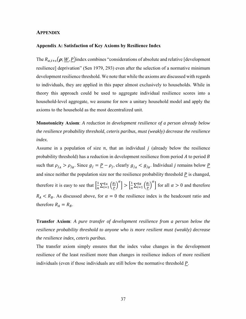
The 𝑅𝛼,𝑡+𝑠(𝝆; 𝑊, 𝑃)index combines “considerations of absolute and relative [development

resilience] deprivation” (Sen 1979, 293) even after the selection of a normative minimum

development resilience threshold. We note that while the axioms are discussed with regards

to individuals, they are applied in this paper almost exclusively to households. While in

theory this approach could be used to aggregate individual resilience scores into a

household-level aggregate, we assume for now a unitary household model and apply the

axioms to the household as the most decentralized unit.

Monotonicity Axiom: A reduction in development resilience of a person already below

the resilience probability threshold, ceteris paribus, must (weakly) decrease the resilience

index.

Assume in a population of size 𝑛, that an individual 𝑗 (already below the resilience

probability threshold) has a reduction in development resilience from period 𝐴 to period 𝐵

such that 𝜌𝑗𝐴> 𝜌𝑗𝐵

. Since 𝑔𝑗 = 𝑃 − 𝜌𝑗 , clearly 𝑔𝑗𝐴< 𝑔𝑗𝐵

. Individual 𝑗 remains below 𝑃

and since neither the population size nor the resilience probability threshold 𝑃 is changed,

therefore it is easy to see that [1

𝑛∑ (

𝑔𝑖

𝑃)

𝛼𝑞𝐴𝑖=1 ] > [

1

𝑛∑ (

𝑔𝑖

𝑃)

𝛼𝑞𝐵𝑖=1 ] for all 𝛼 > 0 and therefore

𝑅𝐴 < 𝑅𝐵. As discussed above, for 𝛼 = 0 the resilience index is the headcount ratio and

therefore 𝑅𝐴 = 𝑅𝐵.

Transfer Axiom: A pure transfer of development resilience from a person below the

resilience probability threshold to anyone who is more resilient must (weakly) decrease

the resilience index, ceteris paribus.

The transfer axiom simply ensures that the index value changes in the development

resilience of the least resilient more than changes in resilience indices of more resilient

individuals (even if those individuals are still below the normative threshold 𝑃.

38

Case 1: If the transfer is made to someone with resilience above 𝑃, this is effectively

equivalent to the monotonicity axiom above.

Case 2: Let two individuals 𝑗 and 𝑘 each have a level of development resilience below the

resilience probability threshold, such that 𝜌𝑗𝐴< 𝜌𝑘𝐴

≤ 𝑃 in period 𝐴. A pure resilience

transfer in the amount of 𝜋 reduces the development resilience of person 𝑗 to 𝜌𝑗𝐵= 𝜌𝑗𝐴

−

𝜋 in period 𝐵 and increases the resilience of person 𝑘 to 𝜌𝑘𝐵= 𝜌𝑘𝐴

+ 𝜋, which may or may

not be above 𝑃.

Case 2a: For this subcase let 𝜌𝑘𝐵= 𝜌𝑘𝐴

+ 𝜋 ≤ 𝑃, so individual 𝑗’s gap has increased

(𝑔𝑗𝐴< 𝑔𝑗𝐵

) and 𝑘’s gap has shrunken (𝑔𝑘𝐴> 𝑔𝑘𝐵

). It is immediately clear that 𝑅𝐴 = 𝑅𝐵

when 𝛼 = 0 or 𝛼 = 1 since neither the headcount nor the cumulative resilience gap is

altered by the transfer. For 𝛼 > 1, [1

𝑛∑ (

𝑔𝑖

𝑃)

𝛼𝑞𝐴𝑖=1 ] > [

1

𝑛∑ (

𝑔𝑖

𝑃)

𝛼𝑞𝐵𝑖=1 ] since greater weight is

placed on larger gaps and therefore it follows that 𝑅𝐴 < 𝑅𝐵.

Case 2b: Now let 𝜌𝑘𝐵= 𝜌𝑘𝐴

+ 𝜋 > 𝑃. Notice that for 𝛼 = 0, the headcount ratio, 𝑅𝐴 > 𝑅𝐵

since fewer individuals fall below the resilience probability threshold. However, for ≥ 1 ,

[1

𝑛∑ (

𝑔𝑖

𝑃)

𝛼𝑞𝐴𝑖=1 ] > [

1

𝑛∑ (

𝑔𝑖

𝑃)

𝛼𝑞𝐵𝑖=1 ] as individual 𝑗’s gap increases (𝑔𝑗𝐴

+ 𝜋 = 𝑔𝑗𝐵) and 𝑘

surpasses the threshold and is considered resilient (𝑔𝑘𝐵= 0), implying 𝑅𝐴 < 𝑅𝐵.

Relative Equity Axiom: If person 𝑗 is accepted to be less resilient than person 𝑘 in a given

resilience configuration 𝝆, then the weight on the resilience gap 𝑔𝑗 of the less resilient

person 𝑗 should be greater than the weight on the resilience gap 𝑔𝑘.

While the headcount ratio with 𝛼 = 0 ignores resilience gaps completely and gaps are

given equal weights when 𝛼 = 1, for all 𝛼 > 1 the resilience index 𝑅(𝝆; 𝑊, 𝑃) ≡ 1 −

[1

𝑛∑ (

𝑔𝑖

𝑃)

𝛼𝑞𝑖=1 ] weighs larger gaps more heavily than smaller gaps.

Decomposability: The resilience index is decomposable with population share weights.

39

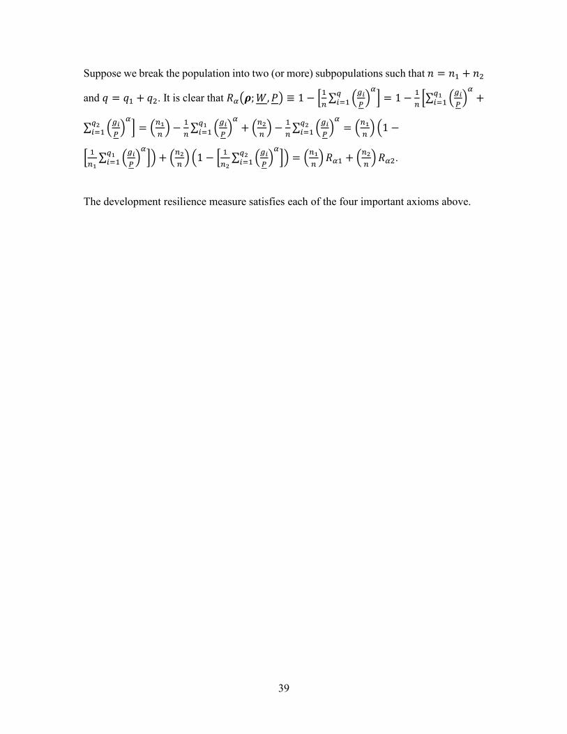
Suppose we break the population into two (or more) subpopulations such that 𝑛 = 𝑛1 + 𝑛2

and 𝑞 = 𝑞1 + 𝑞2. It is clear that 𝑅𝛼(𝝆; 𝑊, 𝑃) ≡ 1 − [1

𝑛∑ (

𝑔𝑖

𝑃)

𝛼𝑞𝑖=1 ] = 1 −

1

𝑛[∑ (

𝑔𝑖

𝑃)

𝛼𝑞1𝑖=1 +

∑ (𝑔𝑖

𝑃)

𝛼𝑞2𝑖=1 ] = (

𝑛1

𝑛) −

1

𝑛∑ (

𝑔𝑖

𝑃)

𝛼𝑞1𝑖=1 + (

𝑛2

𝑛) −

1

𝑛∑ (

𝑔𝑖

𝑃)

𝛼𝑞2𝑖=1 = (

𝑛1

𝑛) (1 −

[1

𝑛1∑ (

𝑔𝑖

𝑃)

𝛼𝑞1𝑖=1 ]) + (

𝑛2

𝑛) (1 − [

1

𝑛2∑ (

𝑔𝑖

𝑃)

𝛼𝑞2𝑖=1 ]) = (

𝑛1

𝑛) 𝑅𝛼1 + (

𝑛2

𝑛) 𝑅𝛼2.

The development resilience measure satisfies each of the four important axioms above.

40

Appendix B: Robustness

Table B1: Poisson Estimates of TLU Well-Being – Polynomial Specifications

VARIABLES (1) (2) (3) (4) (5) (6) (7) (8)

TLU TLU TLU TLU TLU TLU TLU TLU

TLUt−1 1.55*** 3.43*** 5.73*** 9.69*** 12.2*** 20.0*** 22.2*** 27.5***

(∗ 102) (-0. 145) (0. 606) (0.556) (0.396) (0.978) (1.14) (1.21) (1.47)

TLUt−12 -0.0864**

-0.

36***

-

1.21***

-

2.08***

-

5.82*** -7.28***

-

11.4***

(∗ 103) (0.0436) (0.0759) (0.0865) (0.343) (0.604) (0.717) (1.05)

TLUt−13 0.646*** 5.80*** 15.8*** 82.4*** 119*** 243***

(∗ 106) (0.167) (0.500) ( 4.06) (12.2) (16.6) (31.2)

TLUt−14

-

0.86***

-

5.19***

-

56.6*** -98.7***

-

280***

(∗ 108) (0.0810) (1.80) (10.7) ( 17.5) (44.7)

TLUt−15 1.00** 18.0*** 42.3*** 180***

(∗ 1010) (0.252) (3.98) (8.81) (33.7)

TLUt−16

-

2.08*** -8.81***

-

64.6***

(∗ 1012) (0.507) (2.06) (13.6)

TLUt−17 0.702*** 12.0***

(∗ 1014) (0.179) (2.74)

TLUt−18

-

8.97***

(∗ 1017) (2.17)

Controls Y Y Y Y Y Y Y Y

AIC 136.2 119.5 109.2 99.0 97.1 91.3 90.3 89.2

T-test1 0.0211** 0.0000*** 0.0143** 0.1244 0.575 0.3557 0.3369 -

Robust standard errors in parentheses. *** p<0.01, ** p<0.05, * p<0.10

1 P-value of the t-test on the equality of means between predicted values from the specific estimation and

the 8th order polynomial specification.

41

Table B2: Marginal Effects at Representative Values – A Comparison of Two Well-

Being Distributions

(1) (2)

VARIABLES TLU Resilience [~Γ, W=6]2 TLU Resilience [~lnN, W=6]3

low low low low mean high

TLUt−1 0.0616*** 0.0381*** 0.0204*** 0.0613*** 0.0353*** 0.0194***

(0.000494) (0.000236) (0.000311) (0.000461) (0.000830) (0.000475)

Drought -0.181*** -0.112*** -0.0600*** -0.149*** -0.0925*** -0.0535***

(0.00284) (0.00225) (0.00168) (0.00482) (0.00314) (0.00213)

Female Head -0.122*** -0.0756*** -0.0406*** -0.0860*** -0.0535*** -0.0310***

(0.00455) (0.00301) (0.00178) (0.00451) (0.00297) (0.00178)

Head Age 0.0684*** 0.0423*** 0.0227*** 0.0142 0.00774 0.00413 (∗ 102) (0.0141) (0.00864) (0.00461) (0.0145) (0.00900) (0.00521)

Education in 0.00433*** 0.00268*** 0.00144*** 0.000777 0.000483 0.000280

Yrs (0.00107) (0.000655) (0.000351) (0.000712) (0.000443) (0.000256)

Dependency -0.0564*** -0.0349*** -0.0187*** -0.0453*** -0.0282*** -0.0163***

Ratio (0.00212) (0.00142) (0.000868) (0.00225) (0.00145) (0.000928)

Religion &

Nomadic

Dummies

Y Y Y Y Y Y

Model BIC -28669.092 2727.261

Bootstrapped4 (1) and robust (2) standard errors in parentheses. Pooled Sample, n = 3,581.

*** p<0.01, ** p<0.05, * p<0.10

2 These are the same estimates as presented in Table 2 column (3).

3 Distribution parameters for the lognormal distribution are: 𝑊𝑡|𝑊𝑡−1~ln𝑁 (ln(𝜇1𝑡) −1

2ln (1 +

𝜇2𝑡

𝜇1𝑡2 ) , ln (1 +

𝜇2𝑡

𝜇1𝑡2 )). Given convergence issues with the estimator, these estimates are not bootstrapped and

exclude survey weights. The specification was also only able to include a third order polynomial. The

fractional response model uses a logit model for the conditional mean. 4 B=400 repetitions chosen for the bootstrap based on Cameron & Trivedi (2010, p. 433).

42

Table B3: OLS Estimates of TLU Well-Being

(1) (2) (3)

VARIABLES IHS5(TLU) Variance

(IHS(TLU))

Resilience

[~Γ, W=6]

TLUt−1 0.155*** -0.0160** 0.00626***

(0.00577) (0.00775) (0.00101)

TLUt−12 (∗ 1000) -2.40*** 0.395 -0.0994**

(0.172) (0.336) (0.0477)

TLUt−13 (∗ 106) 12.8*** -1.75 0.563

(1.35) (4.34) (0.647)

TLUt−14 (∗ 109) -20.1*** 2.17 -0.917

(2.54) (16.4) (2.55)

Drought -0.164*** 0.0551 -0.00529***

(0.0404) (0.0477) (0.000852)

Female Head (=1) -0.234*** 0.107** -0.0133***

(0.0460) (0.0452) (0.00149)

Head Age 0.0161** -0.00185 0.000787***

(0.00753) (0.00802) (0.000220)

Head Age2(∗ 105) -15.7** 3.33 -0.841***

(6.97) (7.32) (0.199)

Education in Yrs -0.00753 0.0145* -0.000463*

(0.00925) (0.00859) (0.000263)

Dependency Ratio 1.42 -0.0956 0.0111 (∗ 100) (2.29) (2.05) (0.0584)

Religion &

Settled

Dummies

Y Y Y

Constant 0.827*** 0.668*** 0.0278***

5 The inverse hyperbolic sine of TLU.

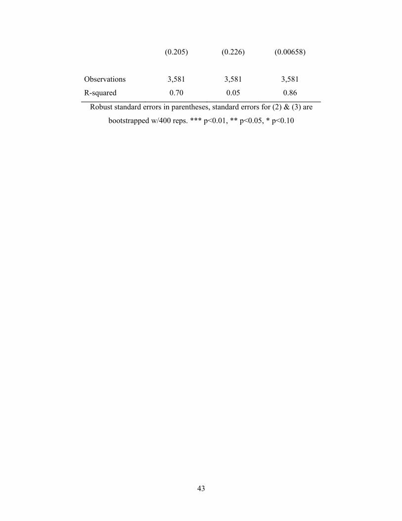
43

(0.205) (0.226) (0.00658)

Observations 3,581 3,581 3,581

R-squared 0.70 0.05 0.86

Robust standard errors in parentheses, standard errors for (2) & (3) are

bootstrapped w/400 reps. *** p<0.01, ** p<0.05, * p<0.10

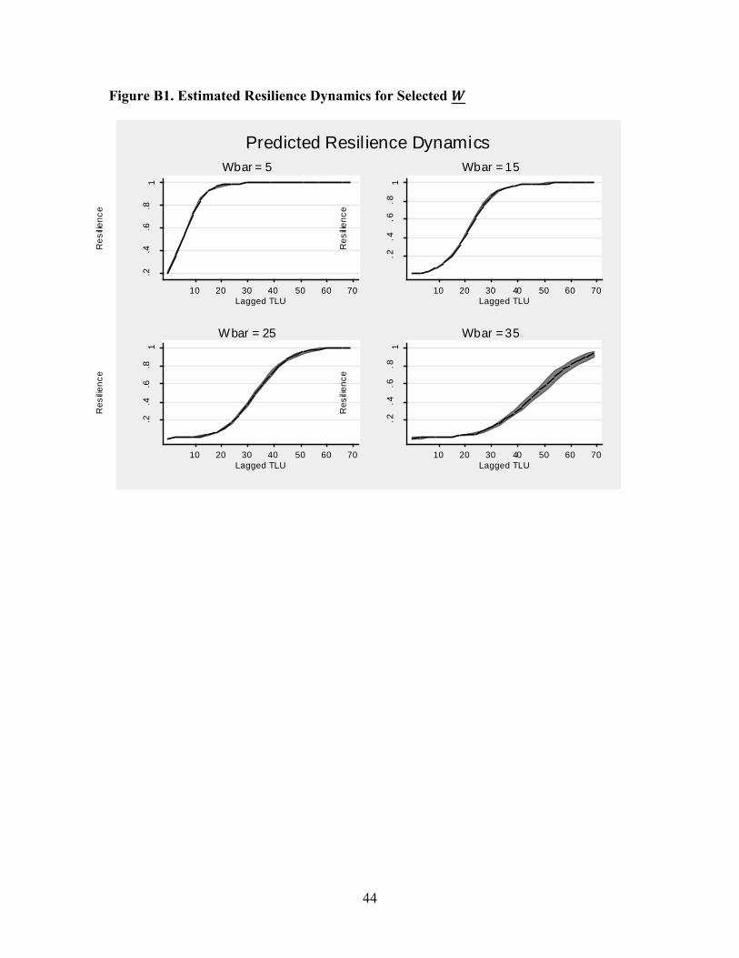
44

Figure B1. Estimated Resilience Dynamics for Selected 𝑾

.2.4

.6.8

1

Re

sili

en

ce

10 20 30 40 50 60 70

Lagged TLU

Wbar = 5

.2.4

.6.8

1

Re

sili

en

ce

10 20 30 40 50 60 70

Lagged TLU

Wbar = 15

.2.4

.6.8

1

Re

sili

en

ce

10 20 30 40 50 60 70

Lagged TLU

Wbar = 25

.2.4

.6.8

1

Re

sili

en

ce

10 20 30 40 50 60 70

Lagged TLU

Wbar = 35

Predicted Resilience Dynamics

Recent Publications in the Series

nº Year Author(s) Title

235 2016 las Gerber and Julia Anna Matz Social networks, agricultural innovations, and farm productivity

in Ethiopia

234 2016 Megan Sheahan, Christopher B. Barrett

and Casey Goldvale

The unintended consequences of agricultural input

intensification: Human health implications of agro-chemical use

in Sub-Saharan Africa

233 2015 Adamon N. Mukasa Technology Adoption and Risk Exposure among Smallholder

Farmers: Panel Data Evidence from Tanzania and Uganda

232 2015 Linguère Mously Mbaye Remittances and Access to Rural Credit Markets: Evidence from

Senegal

231 2015 Adamon N. Mukasa and Adeleke O. Salami Gender productivity differentials among smallholder farmers in

Africa: A cross-country comparison

230 2015 Valérie Bérenger and Audrey Verdier-

Chouchane

Child Labour and Schooling in South Sudan and Sudan:

Is There a Gender Preference?

229 2015 Luc Christiaensen and Jonathan Kaminski Structural change, economic growth and poverty reduction –

Micro-evidence from Uganda

228 2015 Mouhamadou Sy Overborrowing and Balance of Payments Imbalances in a

Monetary Union

227 2015 Mthuli Ncube and Zuzana Brixiová Public Debt Sustainability in Africa: Building Resilience and

Challenges Ahead

226 2015 Elphas Ojiambo, Jacob Oduor, Tom Mburu

and Nelson Wawire Aid Unpredictability and Economic Growth in Kenya