Embed Size (px)
Citation preview

ESTIMATING DESIGN-FLOOD DISCHARGES FOR STREAMS IN IOWA USING DRAINAGE-BASIN AND CHANNEL-GEOMETRY CHARACTERISTICS
By David A. Eash_______________________________
U.S. GEOLOGICAL SURVEY Water-Resources Investigations Report 93-4062
Prepared in cooperation with theIOWA HIGHWAY RESEARCH BOARDand the HIGHWAY DIVISION of theIOWA DEPARTMENT OF TRANSPORTATION(Iowa DOT Research Project HR-322)
Iowa City, Iowa 1993

U.S. DEPARTMENT OF THE INTERIOR
BRUCE BABBITT, Secretary
U.S. GEOLOGICAL SURVEY
Robert M. Hirsch, Acting Director
For additional information write to:
District Chief U.S. Geological Survey Rm. 269, Federal Building 400 South Clinton Street Iowa City, Iowa 52244
Copies of this report can be purchased from:
U.S. Geological Survey Books and Open-File Reports Federal Center, Bldg. 810 Box 25425 Denver, Colorado 80225
ii ESTIMATING DESIGN-FLOOD DISCHARGES FOR STREAMS IN IOWA

CONTENTS
Page
Abstract...........................................................................................................^^Introduction....................................................................................................................................!
Purpose and scope.............................................................................................................2Acknowledgments .............................................................................................................3
Flood-frequency analyses of streamflow-gaging stations in Iowa...............................................3Development of multiple-regression equations............................................................................6
Ordinary least-squares regression...................................................................................6Weighted least-squares regression..................................................................................8
Estimating design-flood discharges using drainage-basin characteristics................................^
Geographic-information-system procedure................................................................... 10Verification of drainage-basin characteristics............................................................... 13Drainage-basin characteristic equations....................................................................... 16Example of equation use-example 1 .............................................................................18
Estimating design-flood discharges using channel-geometry characteristics.......................... 19
Channel-geometry data collection.................................................................................. 19Channel-geometry characteristic equations.................................................................. 22
Analysis of channel-geometry data on a statewide basis................................. 22Analysis of channel-geometry data by selected regions................................... 22Comparison of regional and statewide channel-geometry equations.............. 24
Examples of equation use examples 2-4....................................................................... 27
Application and reliability of flood-estimation methods............................................................ 32
'" Limitations and accuracy of equations ..........................................................................32Weighting design-flood discharge estimates .................................................................34
Calculation of estimates ....................................................................................35Example of weighting example 5.....................................................................35
Weighting design-flood discharge estimates for gaged sites ........................................35
Calculation of estimates ....................................................................................36Examples of weighting-examples 6-7............................................................... 36
Estimating design-flood discharges for an ungaged site on a gaged stream...............37
Calculation of estimates ....................................................................................37Example of estimation method-example 8 ......................................................38
Summary and conclusions...........................................................................................................41References......................................................................................................:.......................... ....42
CONTENTS iii

CONTENTS-Continued
Page
Appendix A. Selected drainage-basin characteristics quantified using a geographic-information-system procedure..............................................................................45
Appendix B. Techniques for manual, topographic-map measurements of primarydrainage-basin characteristics used in the regression equations....................... 49
Appendix C. Procedure for conducting channel-geometry measurements ..............................53
ILLUSTRATIONS
Page
Figure 1. Map showing location of streamflow-gaging stations used to collectdrainage-basin data.............................................................................................4
2. Map showing location of streamflow-gaging stations used to collect channel-geometry data and regional transition zone......................................... 5
3. Graph showing example of a flood-frequency curve........................................... 7
4. Map showing four geographic-information-system maps that constitute a digital representation of selected aspects of a drainage basin........................ 11
5. Map showing distribution of 2-year, 24-hour precipitation intensity for Iowa and southern Minnesota........................................................................... 13
6. Block diagram of a typical stream channel ......................................................20
7. Photographs showing active-channel and bankfull reference levels at six streamflow-gaging stations in Iowa.................................................................. 21
8. Graphs showing relation between 2-year recurrence-interval discharge and channel width for bankfull and active-channel width regression equations ............................................................................................................28
9. Graphs showing relation between 100-year recurrence-interval discharge and channel width for bankfull and active-channel width regression equations ............................................................................................................29
10. Graph showing bankfull cross section for Black Hawk Creek at GrundyCenter.................................................................................................................31
iv ESTIMATING DESIGN-FLOOD DISCHARGES FOR STREAMS IN IOWA

TABLES
Page
Table 1. Comparisons of manual measurements and geographic-information- system-procedure measurements of selected drainage-basin characteristics at selected streamflow-gaging stations ................................... 14
2. Statewide drainage-basin characteristic equations for estimating design- flood discharges in Iowa..................................................................................... 17
3. Statewide channel-geometry characteristic equations for estimating design-flood discharges in Iowa.........................................................................23
4. Region I channel-geometry characteristic equations for estimating design- flood discharges in Iowa outside of the Des Moines Lobe landform region..................................................................................................................25
5. Region II channel-geometry characteristic equations for estimating design- flood discharges in Iowa within the Des Moines Lobe landform region .........26
6. Statistical summary for selected statewide drainage-basin and channel- geometry characteristics, and for selected regional channel-geometry characteristics at streamflow-gaging stations in Iowa.................................... 33
7. Comparisons of manual measurements made from different scales of topographic maps of primary drainage-basin characteristics used in the regression equations ..........................................................................................50
8. Flood-frequency data for streamflow-gaging stations in Iowa........................ 57
9. Selected drainage-basin and channel-geometry characteristics for streamflow-gaging stations in Iowa ..................................................................80
TABLES v

CONVERSION FACTORS, ABBREVIATIONS, AND VERTICAL DATUM
Multiply By To obtain
inch (in.) 25.4 millimeter
foot (ft) 0.3048 meter
mile (mi) 1.609 kilometer
square mile (mi2) - 2.590 square kilometer
foot per mile (ft/mi) 0.1894 meter per kilometer
mile per square mile (mi/mi2) 0.621 kilometer per square
kilometer
cubic foot per second (ft3/s) 0.02832 cubic meter per second
Sea level: In this report, "sea level" refers to the National Geodetic Vertical Datum of 1929
a geodetic datum derived from a general adjustment of the first-order level nets of the United States
and Canada, formerly called Sea Level Datum of 1929.
vi ESTIMATING DESIGN-FLOOD DISCHARGES FOR STREAMS IN IOWA

ESTIMATING DESIGN-FLOOD DISCHARGES FOR STREAMS IN IOWA USING DRAINAGE-BASIN AND CHANNEL-GEOMETRY
CHARACTERISTICS
By David A. Eash
ABSTRACT
Drainage-basin and channel-geometry multiple-regression equations are presented for estimating design-flood discharges having recurrence intervals of 2, 5, 10, 25, 50, and 100 years at stream sites on rural, unregulated streams in Iowa. Design-flood discharge estimates determined by Pearson Type-Ill analyses using data collected through the 1990 water year are reported for the 188 streamflow-gaging stations used in either the drainage-basin or channel-geometry regression analyses. Ordinary least-squares multiple-regression techniques were used to identify selected drainage-basin and channel-geometry characteristics and to delineate two channel-geometry regions. Weighted least- squares multiple-regression techniques, which account for differences in the variance of flows at different gaging stations and for variable lengths in station records, were used to estimate the regression parameters.
Statewide drainage-basin equations were developed from analyses of 164 streamflow- gaging stations. Drainage-basin characteristics were quantified using a geographic-information- system procedure to process topographic maps and digital cartographic data. The significant characteristics identified for the drainage-basin
^equations included contributing drainage area, relative relief, drainage frequency, and 2-year, 24-hour precipitation intensity. The average standard errors of prediction for the drainage- basin equations ranged from 38.6 to 50.2 percent. The geographic-information-system procedure expanded the capability to quantitatively relate drainage-basin characteristics to the magnitude and frequency of floods for stream sites in Iowa and provides a flood-estimation method that is independent of hydrologic regionalization.
Statewide and regional channel-geometry regression equations were developed from analyses of 157 streamflow-gaging stations. Channel-geometry characteristics were measured
onsite and on topographic maps. Statewide and regional channel-geometry regression equations that are dependent on whether a stream has been channelized were developed on the basis of bankfull and active-channel characteristics. The significant channel-geometry characteristics identified for the statewide and regional regression equations included bankfull width and bankfull depth for natural channels unaffected by channel ization, and active-channel width for stabilized channels affected by channelization. The average standard errors of prediction ranged from 41.0 to 68.4 percent for the statewide channel-geometry equations and from 30.3 to 70.0 percent for the regional channel-geometry equations.
Procedures provided for applying the drainage-basin and channel-geometry regression equations depend on whether the design-flood discharge estimate is for a site on an ungaged stream, an ungaged site on a gaged stream, or a gaged site. When both a drainage-basin and a channel-geometry regression-equation estimate are available for a stream site, a procedure is presented for determining a weighted average of the two flood estimates. The drainage-basin regression equations are applicable to unregu lated rural drainage areas less than 1,060 square miles, and the channel-geometry regression equations are applicable to unregulated rural streams in Iowa with stabilized channels.
INTRODUCTION
Knowledge of the magnitude and frequency of floods is essential for the effective manage ment of flood plains and for the economical planning and safe design of bridges, culverts, levees, and other structures located along streams. Long-term flood data collected from a network of streamflow-gaging stations operated in Iowa are available for hydrologic analysis to compute design-flood discharge estimates for the gaged sites as well as for ungaged sites on the gaged streams. Techniques are needed to estimate design-flood discharges for sites on all
INTRODUCTION 1

ungaged streams in Iowa because most such stream sites in the State have no flood data available, particularly sites on smaller streams.
Flood runoff is a function of many interrelated factors that include, but are not limited to climate, soils, land use, and the physiography of drainage basins. Previous investigations for Iowa (Schwob, 1953, 1966; Lara, 1973, 1987) have been limited to the types of basin characteristics that can be investigated as potential explanatory variables for the development of multiple-regression flood- estimation equations because many of the flood-runoff factors are difficult to measure. Previous investigations defined hydrologic regions to account for factors affecting flood runoff that were difficult to measure directly. The hydrologic regions were delineated on the basis of physiographic differences of broad geographic landform regions. However, two major limitations are encountered when using the hydrologic-region method to estimate flood discharges for ungaged sites. First, it is difficult to weight flood estimates for drainage basins located in more than one hydrologic region or located near the boundaries of hydrologic regions because the boundaries are not well defined. Regional boundaries are transitional zones where the physiographic characteristics of one hydrologic region gradually merge into another. Second, because large hydrologic regions may contain drainage basins with physiographies that are anomalous to the region in which they are located, it is difficult to correlate their physiographic differences to another hydrologic region, or to weight their flood estimates. Quantitative measurements of basin morphology to determine appropriate regional equations for drainage basins are not applicable for resolving these regional limitations. As a result, flood estimates for some ungaged sites become very subjective.
To address the need to minimize the subjectivity encountered in applying regional flood-estimation methods, a study using two different flood-estimation methods was made by the U.S. Geological Survey in cooperation with the Iowa Highway Research Board and the Highway Division of the Iowa Department of Transportation. Two new flood-estimation methods for Iowa, which are presumed to be independent from each other, were used in this
study. An advantage in developing flood- frequency equations using two independent flood-estimation methods is that each method can be used to verify the results of the other, and the estimates obtained from each method can be used to calculate a weighted average.
Methods are now available to more easily quantify selected morphologic and climatic characteristics for a large number of drainage basins. A geographic-information-system (GIS) procedure developed by the U.S. Geological Survey uses topographic maps and digital cartographic data to quantify several basin characteristics that typically were not quantified previously. This GIS procedure expands the capability to relate drainage-basin characteristics to the magnitude and frequency of floods for stream sites in Iowa and provides a flood-estimation method that is independent of hydrologic regionalization.
Measurements of channel-geometry characteristics have been used to estimate the magnitude and frequency of floods in investigations conducted by Fields (1975), Webber and Roberts (1981), Parrett and others (1987), Hedman and Kastner (1977), and Osterkamp and Hedman (1982). These investigations have shown that measurements of specific channel-geometry characteristics provide a reliable method £or estimating flood discharges because channel cross-sectional characteristics are assumed to be a function of flow volume and sediment-load transport (Pickup and Rieger, 1979, p. 41; Osterkamp, 1979, p. 2).
Purpose and Scope
The purpose of this report is to: (1) define equations for Iowa that relate measurable drainage-basin characteristics to design-flood discharges having recurrence intervals of 2, 5, 10, 25, 50, and 100 years that are independent of hydrologic regionalization; (2) define corroborative equations for Iowa that relate channel-geometry characteristics to the same design-flood recurrence intervals; and (3) define application and reliability of drainage-basin and channel-geometry flood-estimation methods.
Both the drainage-basin and channel- geometry flood-estimation methods described in
2 ESTIMATING DESIGN-FLOOD DISCHARGES FOR STREAMS IN IOWA

this report are applicable to unregulated rural streams located within the State. The drainage-basin flood-estimation method is limited to streams with drainage areas less than 1,060 mi2 . The channel-geometry flood- estimation method is applicable to stabilized stream channels in Iowa.
Acknowledgments
The U.S. Army Corps of Engineers, Omaha and Rock Island Districts, contributed to the funding of the sediment-sample analyses. James J. Majure, formerly with the U.S. Geological Survey, Iowa City, Iowa, and now with the Iowa State University, GIS Support and Research Facility, Ames, Iowa, developed the computer software used to quantify the drainage-basin characteristics and the software used to integrate the overall GIS procedure.
FLOOD-FREQUENCY ANALYSES OF STREAMFLOW-GAGING STATIONS IN IOWA
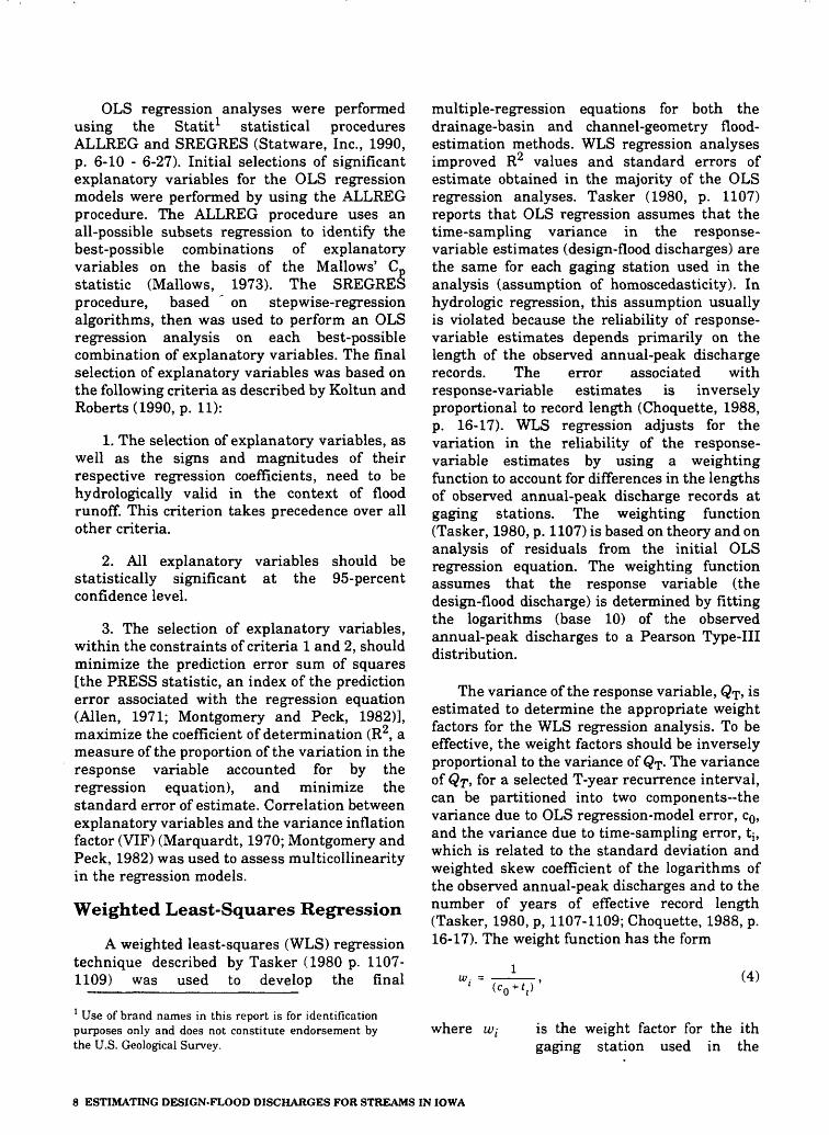
Flood-frequency curves were developed for 188 streamflow-gaging stations operated in Iowa by the U.S. Geological Survey. They were developed according to procedures outlined in Bulletin 17B of the Interagency Advisory Committee on Water Data (IACWD, 1982, p. 1-28). These flood-frequency curves include data collected through the 1990 water year for both active and discontinued continuous-record and crest-stage gaging stations having at least 10 years of gaged annual-peak discharges. A water year is the 12-month period from October 1 through September 30 and is designated by the calendar year in which it ends. The locations of the 164 gaging stations studied using the drainage-basin flood-estimation method are shown in figure 1, and the locations of the 157 gaging stations studied using the channel- geometry flood-estimation method are shown in figure 2. Map numbers for the gaging stations shown in figures 1 and 2 are referenced to gaging-station numbers and names in tables 8 and 9 (at end of this report). The observed annual-peak discharge record at each site includes water years during which the gaging station was operated, which is termed the systematic period of record. The observed annual-peak discharge record also may include historic-peak discharges that occurred during
water years outside the systematic period of record.
A flood-frequency curve relates observed annual-peak discharges to annual exceedance probability or recurrence interval. Annual exceedance probability is expressed as the chance that a given flood magnitude will be exceeded in any 1 year. Recurrence interval, which is the reciprocal of the annual exceedance probability, is the average number of years between exceedances of a given flood magnitude. For example, a flood with a magnitude that is expected to be exceeded once on the average during any 100-year period (recurrence interval) has a 1-percent chance (annual exceedance probability = 0.01) of being exceeded during any 1 year. This flood, commonly termed the 100-year flood, is generally used as a standard against which flood peaks are measured. Although the recurrence interval represents the long-term average period between floods of a specific magnitude, rare floods could occur at shorter intervals or even within the same year.
Flood-frequency curves were developed by fitting the logarithms (base 10) of the observed annual-peak discharges to a Pearson Type-Ill distribution using U.S. Geological Survey WATSTORE flood-frequency analysis programs (Kirby, 1981, p. C1-C57). Extremely small discharge, values (low outliers) were censored, adjustments were made for extremely large discharge values (high outliers), and the coefficient of skew was weighted for each gaging station with skew values obtained from a generalized skew-coefficient map (IACWD, 1982). Whenever possible, historically adjusted flood-frequency curves were developed to extend the flood record for gaging stations with historic peak-flood information.
The recommended equation (IACWD, 1982, p. 9) for fitting a Pearson Type-Ill distribution to the logarithms of observed annual-peak discharges of a gaging station is
log(QT , ffJ = x + ks, (1)
where QT(#) *s ^ne design-flood discharge for a gage, in cubic feet per second, for a selected T-year recurrence
FLOOD-FREQUENCY ANALYSES OF STREAMFLOW-GAGING STATIONS IN IOWA 3

^
- "
- -*
- - *i
i-u
zz:"
- LL
. .. _
/i _
_i_
_ J
T'T
* i"
_ _
_ _
- .
\ B
ase
from
U.S
. Geo
logi
cal S
urve
y di
gita
l dat
a,
MlS
SO
Uri
0
20
40
60 M
ILE
S
\ 1:
2,00
0,00
0.19
79
|
__
__
__
tZo
Se61
?ITr
anSV
efSe
Mef
Cal
0fPr
o|eC
tl0n
' °
20
40
60 K
ILO
ME
TER
S
EX
PL
AN
AT
ION
164A
U.S
. G
EO
LOG
ICA
L S
UR
VE
Y S
TR
EA
MF
LOW
-GA
GIN
GS
TA
TIO
N A
ND
DO
WN
ST
RE
AM
-OR
DE
R M
AP
NU
MB
ER
- m
ap n
umbe
rs a
re r
efer
ence
d in
tabl
es 8
and
9
Figu
re 1
. Lo
catio
n of
stre
amflo
w-g
agin
g st
atio
ns u
sed
to c
olle
ct d
rain
age-
basi
n da
ta.

DE
S M
OIN
ES
LO
BE
LA
ND
FO
RM
RE
GIO
N
\ B
ase
Irom
U.S
. G
eolo
gica
l Sur
vey
digi
tal d
ala.
M
isso
uri
0
\ 1:
2.00
0.00
0. 1
979
j_U
nive
rsal
Tra
nsve
rse
Mer
cato
r pro
ject
ion.
Q
20
40
60 K
ILO
ME
TE
RS
Zone
15
,
EX
PL
AN
AT
ION
'
K
RE
GIO
NA
L T
RA
NS
ITIO
N Z
ON
E
117A
U
.S.
GE
OLO
GIC
AL
SU
RV
EY
ST
RE
AM
FLO
W-G
AG
ING
ST
AT
ION
AN
D D
OW
NS
TR
EA
M-O
RD
ER
MA
P N
UM
BE
R--
M
ap n
umbe
rs a
re r
efer
ence
d in
tabl
es 8
and
9
II
CH
ANN
EL-G
EOM
ETR
Y, H
YDR
OLO
GIC
-REG
ION
NU
MBE
R
Fig
ure
2.
Loca
tion
of s
trea
mflo
w-g
agin
g st
atio
ns u
sed
to c
olle
ct c
hann
el-g
eom
etry
dat
a an
d re
gion
al t
rans
ition
zon
e.

interval;
x is the mean of the logarithms (base 10) of the observed annual-peak discharges;
k is the standardized Pearson Type-Ill deviate for a selected T-year recurrence interval and weighted skew coefficient; and
s is the standard deviation of the logarithms (base 10) of the observed annual-peak dis charges.
Results of the Pearson Type-Ill flood- frequency analyses are presented in table 8 (listed as method B17B, at end of this report) for the 188 streamflow-gaging stations analyzed using either the drainage-basin or channel- geometry flood-estimation techniques. Included in table 8 is information about the type of gage operated, the effective record length of the gage, whether a systematic or historical analysis was performed, the observed annual-peak discharge record (listed as flood period), and the maximum known flood-peak discharge and its recurrence interval. An example flood-frequency curve is shown in figure 3.
DEVELOPMENT OFMULTIPLE-REGRESSIONEQUATIONS
Multiple linear-regression techniques were used to independently relate selected drainage- basin and channel-geometry characteristics to design-flood discharges having recurrence intervals of 2, 5, 10, 25, 50, and 100 years. A general overview of the ordinary least-squares and weighted least-squares multiple linear- regression techniques used to develop the equations is presented in the following two sections. Specific information on the multiple- regression analyses for either flood-estimation method is presented in later sections entitled "Drainage-Basin Characteristic Equations" and "Channel-Geometry Characteristic Equations."
Ordinary Least-Squares Regression
Ordinary least-squares (OLS) multiple linear-regression techniques were used to
develop the initial multiple-regression equations, or models, for both the drainage- basin and channel-geometry flood-estimation methods. In OLS regression, a design-flood discharge (termed the response variable) is estimated on the basis of one or more significant drainage-basin or channel-geometry character istics (termed the explanatory variables) in which each observation is given an equal weight. The response variable is assumed to be a linear function of one or more of the explanatory variables. Logarithmic transforma tions (base 10) were performed for both the response and explanatory variables used in all of the OLS regression analyses. Data transformations were used to obtain a more constant variance of the residuals about the regression line and to linearize the relation between the response variable and explanatory variables. The general form of the OLS regres sion equations developed in these analyses is
log 10 (QT ) = log 10 (C) +
62log 10 (X2) + ... + 6p log
(2)
where Q? is the response variable, the estimated design-flood discharge, in cubic feet per second, for a selected T-year recurrence interval;
C is a constant;
6j is the regression coefficient for the ith explanatory variable (i =
is the value of the ith explanatory variable, a drainage-basin or channel-geometry characteristic (i = 1, ... ,p); and
is the total number of explanatory variables in the equation.
Equation 2, when untransformed, algebraically equivalent to
s
(3)
6 ESTIMATING DESIGN-FLOOD DISCHARGES FOR STREAMS IN IOWA

20,0
00
Q O
O UJ
CO cc LU
C
L
H
LU
UJ
U_ O
CQ ZD
O UJ o cc
< o CO
Q
10,0
00
1,00
0
200
Iv
21
AN
NU
AL
PE
AK
S
X/*
X/
>
/;/
r
^r
S
^r
xX
X
*-
. ^*
X
/
»
*x
s /
^^
X"
^^
J^
ME
AN
LO
GS
3.
411
ST
AN
DA
RD
DE
VIA
TIO
N
0.33
4 S
KE
WN
ES
S C
OE
FF
ICIE
NT
-0
.390
DIS
CH
AR
GE
R
EC
UR
RE
NC
E
(CU
BIC
FE
ET
INT
ER
VA
L P
ER
SE
CO
ND
)
100
YE
AR
12
,400
50
YE
AR
10
,600
25
YE
AR
8,
890
10 Y
EA
R
6,65
0 5
YE
AR
4,
970
2 Y
EA
R
2,71
0
99.0
95.0
90
.0
80.0
70
.0
60.0
50
.0
40.0
30
.0
20.0
EX
CE
ED
AN
CE
PR
OB
AB
ILIT
Y,
IN P
ER
CE
NT
10.0
5.
01.
0 0.
5 0.
2
Pea
rson
Typ
e-Ill
floo
d-fre
quen
cy e
stim
ate
for
stre
amflo
w-g
agin
g st
atio
n 05
4943
00 F
OX
RIV
ER
AT
BLO
OM
FIE
LD (
map
num
ber
133,
fig
ure
1)
Figu
re 3
. E
xam
ple
of a
floo
d-fre
quen
cy c
urve
.
OLS regression analyses were performed using the Statit1 statistical procedures ALLREG and SREGRES (Statware, Inc., 1990, p. 6-10 - 6-27). Initial selections of significant explanatory variables for the OLS regression models were performed by using the ALLREG procedure. The ALLREG procedure uses an all-possible subsets regression to identify the best-possible combinations of explanatory variables on the basis of the Mallows' Cp statistic (Mallows, 1973). The SREGRES procedure, based ' on stepwise-regression algorithms, then was used to perform an OLS regression analysis on each best-possible combination of explanatory variables. The final selection of explanatory variables was based on the following criteria as described by Koltun and Roberts (1990, p. 11):
1. The selection of explanatory variables, as well as the signs and magnitudes of their respective regression coefficients, need to be hydrologically valid in the context of flood runoff. This criterion takes precedence over all other criteria.
2. All explanatory variables should be statistically significant at the 95-percent confidence level.
3. The selection of explanatory variables, within the constraints of criteria 1 and 2, should minimize the prediction error sum of squares [the PRESS statistic, an index of the prediction error associated with the regression equation (Alien, 1971; Montgomery and Peck, 1982)], maximize the coefficient of determination (R2 , a measure of the proportion of the variation in the response variable accounted for by the regression equation), and minimize the standard error of estimate. Correlation between explanatory variables and the variance inflation factor (VIF) (Marquardt, 1970; Montgomery and Peck, 1982) was used to assess multicollinearity in the regression models.
Weighted Least-Squares Regression
A weighted least-squares (WLS) regression technique described by Tasker (1980 p. 1107- 1109) was used to develop the final
1 Use of brand names in this report is for identification purposes only and does not constitute endorsement by the U.S. Geological Survey.
multiple-regression equations for both the drainage-basin and channel-geometry flood- estimation methods. WLS regression analyses improved R2 values and standard errors of estimate obtained in the majority of the OLS regression analyses. Tasker (1980, p. 1107) reports that OLS regression assumes that the time-sampling variance in the response- variable estimates (design-flood discharges) are the same for each gaging station used in the analysis (assumption of homoscedasticity). In hydrologic regression, this assumption usually is violated because the reliability of response- variable estimates depends primarily on the length of the observed annual-peak discharge records. The error associated with response-variable estimates is inversely proportional to record length (Choquette, 1988, p. 16-17). WLS regression adjusts for the variation in the reliability of the response- variable estimates by using a weighting function to account for differences in the lengths of observed annual-peak discharge records at gaging stations. The weighting function (Tasker, 1980, p. 1107) is based on theory and on analysis of residuals from the initial OLS regression equation. The weighting function assumes that the response variable (the design-flood discharge) is determined by fitting the logarithms (base 10) of the observed annual-peak discharges to a Pearson Type-Ill distribution.
The variance of the response variable, QT, is estimated to determine the appropriate weight factors for the WLS regression analysis. To be effective, the weight factors should be inversely proportional to the variance of QT- The variance of Qf, for a selected T-year recurrence interval, can be partitioned into two components-the variance due to OLS regression-model error, c0 , and the variance due to time-sampling error, tj, which is related to the standard deviation and weighted skew coefficient of the logarithms of the observed annual-peak discharges and to the number of years of effective record length (Tasker, 1980, p, 1107-1109; Choquette, 1988, p. 16-17). The weight function has the form
(4)
where W{ is the weight factor for the ith gaging station used in the
8 ESTIMATING DESIGN-FLOOD DISCHARGES FOR STREAMS IN IOWA

analysis.
The model error (c0) is estimated by
cn = maximumERLU
(5)
where SE is the standard error of the estimate from the OLS equation;
GI is a constant; and
ERL is the mean effective record length, in years, for all gaging stations used in each respective regression-model data set.
The time-sampling error (tj) is estimated by
(6)
where ERL^-) is the effective record length, in years, for the ith gaging station used in each respective regression-model data set.
The constant, c^, is related to the recurrence interval of the response variable and to the weighted skew coefficient (g) of the observed annual-peak discharges. It is determined by
c, = maximum-2
If(7)
where s is the mean standard deviation of the logarithms (base 10) of the observed annual-peak dis charges;
k is the mean standardized Pearson Type-Ill deviate for selected T-year recurrence interval and mean weighted skew coefficient g (IACWD, 1982, p. 3-1 - 3-27); and
g is the mean weighted skew coefficient of the logarithms (base 10) of the observed annual-peak discharges (IACWD, 1982, p. 12-15).
The values s and g are statewide estimates determined by the averages of the 188
streamflow-gaging stations analyzed using either the drainage-basin or channel-geometry flood-estimation techniques. These estimation methods are based on the assumption that s and g are approximately constant for all the gaging stations in the State.
The effective record length (ERL) of a gaging station is based on an empirical analysis made by Gary D. Tasker (U.S. Geological Survey, written commun., March 1992) of results reported in Tasker and Thomas (1978) and Stedinger and Cohn (1986). It is determined by
ERL =LS+(HST-LS)a, (8)
where LS
HST
is the systematic record length of a gaging station, in years, the number of water years during which the gaging station was operated;
is the historic record length of a gaging station, in years, as used in a Pearson Type-Ill historical flood-frequency analysis; if a systematic flood-frequency analysis was performed, HST = LS; if (HST-LS) > 200, set
(9)
In the last equation, ph = 1.0 (np I HST), and np is the number of historic and extremely large discharge (high-outlier) peaks.
The ERL used in the weighted least-squares regression analyses for each gaging station is listed in table 8 (at end of this report).
ESTIMATING DESIGN-FLOOD DISCHARGES USING DRAINAGE-BASIN CHARACTERISTICS
The drainage-basin flood-estimation method uses selected drainage-basin characteristics to estimate the magnitude and frequency of floods for stream sites in Iowa. Multiple-regression equations were developed by relating significant drainage-basin characteristics to Pearson Type-Ill, design-flood discharges for 164
ESTIMATING DESIGN-FLOOD DISCHARGES USING DRAINAGE-BASIN CHARACTERISTICS 9

streamflow-gaging stations in Iowa (fig. 1). Drainage-basin characteristics were quantified using a GIS procedure to process topographic maps and digital cartographic data. An overview of the GIS procedure is provided in the following section.
Geographic-Information-System Procedure
The GIS procedure developed by the U.S. Geological Survey (USGS) quantifies for each drainage basin the 26 basin characteristics listed in Appendix A (at end of this report). These characteristics were selected for the GIS procedure on the basis of their hypothesized applicability in flood-estimation analysis and their general acceptability as measurements of drainage-basin morphology and climate. Techniques for making manual measurements of selected drainage-basin characteristics from topographic maps are outlined in Appendix B (at end of this report). The GIS procedure uses ARC/INFO computer software and other software developed specifically to integrate with ARC/INFO (Majure and Soenksen, 1991; Eash, 1993).
The GIS procedure entails four main steps: (1) creation of four GIS digital maps (ARC/INFO coverages) from three cartographic data sources, (2) assignment of attribute information to three of the four GIS digital maps, (3) quantification of 24 morphologic basin characteristics from the four GIS digital maps, and (4) quantification of two climatic basin characteristics from two precipitation data sources.
The first step creates four GIS digital maps representing selected aspects of a drainage basin. Examples of these maps are shown in figure 4. The drainage-divide digital map (fig. 4A) is created by delineating the surface-water drainage-divide boundary for a streamflow- gaging station on 1:250,000-scale U.S. Defense Mapping Agency (DMA) topographic maps. This drainage-divide delineation is manually digitized into a polygon digital map using GIS software. If noncontributing drainage areas are identified within the drainage-divide boundary, then each noncontributing drainage area also is delineated and digitized.
The drainage-network digital map (fig. 4B) is created by extracting the drainage network for the basin from l:100,000-scale USGS digital line graph (DLG) data. The extraction process uses GIS software to select and append together the DLG data contained within the drainage-divide polygon.
The elevation-contour digital map (fig. 4C) is created from l:250,000-scale DMA digital elevation model (DEM) data that are referenced to sea level (in meters). GIS software is used to convert the DEM data to a lattice file of point elevations for an area slightly larger than the drainage-divide polygon. This lattice file of point elevations is contoured with a 12-meter (39.372-ft) or smaller contour interval using ARC/INFO software. The contour interval is chosen to provide at least five contours for each drainage basin. GIS software selects the contours contained within the drainage-divide polygon to create the elevation-contour digital map. Elevation contours then are converted to units of feet.
The basin-length digital map (fig. 4D) is created by delineating and digitizing the basin length from l:250,000-scale DMA topographic maps. The basin length characteristic is delineated by first identifying the main channel for the drainage basin on l:100,000-scale topographic maps. The main channel is identified by starting at the basin outlet and proceeding upstream, repetitively selecting the channel that drains the greater area at each stream junction. The most upstream channel is extended to the drainage-divide boundary defined for the drainage-divide digital map. This main channel identified on l:100,000-scale topographic maps is used to define the main channel on l:250,000-scale topographic maps. The basin length is centered along the main-channel, flood-plain valley from basin outlet to basin divide and digitized with as straight a line as possible from the l:250,000-scale maps. When comparing the basin length shown in figure 4D to those stream segments corresponding to the main channel in figure 4.B, it can be seen that the basin length does not include all the sinuosity of the stream segments.
The second step assigns attributes to specific polygon, line-segment, and point
10 ESTIMATING DESIGN-FLOOD DISCHARGES FOR STREAMS IN IOWA

A. Drainage-divide digital map digitized from Waterloo topographic map.
Base from U.S. Defense Mapping Agency, 1:250,000, 1976Universal Transverse Mercator projection, Zone 15
B. Drainage-network digital map extracted from Marshalltown-West digital line graph data, with stream-order numbers.
Base from U.S. Geological Survey digital data, 1:100,000, 1984 Universal Transverse Mercator projection, Zone 15
C. Elevation-contour digital map created from Waterloo-East digital elevation model, sea-level data, with contour intervals at 39.372 feet.
Base from U.S. Defense Mapping Agency, 1:250,000, 1976Universal Transverse Mercator projection, Zone 15
984.300
D. Basin-length digital map digitized from Waterloo topographic map.
Base from U.S. Defense Mapping Agency, 1:250,000, 1976Universal Transverse Mercator projection, Zone 15
0 2.5 5 MILES
2.5 5 KILOMETERS
EXPLANATIONA STREAMFLOW-GAGING STATION
Figure 4. Four geographic-information-system maps that constitute a digital representation of selectedaspects of a drainage basin.
ESTIMATING DESIGN-FLOOD DISCHARGES USING DRAINAGE-BASIN CHARACTERISTICS 11

features in the first three of the four GIS digital maps shown in figure 4. As a prerequisite, the digital maps are edited to ensure that drainage-divide boundaries, stream segments, and the basin-length line segments are connected properly. If noncontributing drainage areas are identified, they are assigned attributes with separate polygon designations so that the basin-characteristic programs can distinguish between contributing and noncontributing areas. Each line segment in the drainage-network digital map is assigned a Strahler stream-order number (Strahler, 1952) and a code indicating whether the line segment represents part of the main channel or a secondary channel. Specific GIS programs have been developed to assign the proper stream- order number to each line segment and to code those line segments representing the main channel. Figure 45 shows the Strahler stream-order numbers for streams in the Black Hawk Creek at Grundy Center (station number 05463090; map number 73, fig. 1) drainage basin. A description on how to order streams using Strahler's method is included in Appendix B (at end of this report).
The line segments in the elevation-contour digital map were assigned elevations from the processing of the DEM data. Line segments overlain by noncontributing drainage-area polygons are assigned attributes designating noncontributing contour segments. Two point attributes are added to the elevation-contour digital map to represent the maximum and minimum elevations of the drainage basin. The maximum basin elevation is defined from the highest DEM-generated contour elevation within the contributing drainage area. The minimum basin elevation is defined at the basin outlet as an interpolated value between the first elevation contour crossing the main channel upstream of the basin outlet and the first elevation contour crossing the main channel downstream of the basin outlet.
The third step uses the four GIS digital maps shown in figure 4 and a set of programs developed by the USGS (Majure and Soenksen, 1991) to quantify the 24 morphologic basin characteristics listed in Appendix A (at end of this report). These basin characteristics include selected measurements of area, length, shape, and topographic relief that define selected
aspects of basin morphology, and several channel characteristics. The programs access the information automatically maintained by the GIS for each of the four digital maps, such as the length of line segments and the area of polygons, as well as the previously described attribute information assigned to the polygon, line-segment, and point features of three of the four GIS digital maps. The GIS programs then use this information to automatically quantify the 24 morphologic basin characteristics.
The fourth step uses a software program developed to quantify the remaining two basin characteristics listed in Appendix A (at end of this report). These two climatic characteristics are quantified using GIS digital maps representing the distributions of mean annual precipitation and 2-year, 24-hour precipitation intensity for the area contributing to all surface-water drainage in Iowa. This area includes a portion of southern Minnesota. The mean annual precipitation digital map was digitized from a contour map for Iowa, supplied by the Iowa Department of Agriculture and Land Stewardship, State Climatology Office (Des Moines), and from a contour map for Minnesota (Baker and Kuehnast, 1978). The 2-year, 24-hour precipitation intensity digital map was digitized from a contour map for Iowa (Waite, 1988, p. 31) and interpolated contours for southern Minnesota that were digitized from a United States contour map (Hershfield, 1961, p. 95). The digital map representing the distribution of 2-year, 24-hour precipitation intensity for Iowa and southern Minnesota is shown in figure 5. The weighted average for each climatic characteristic is computed for a drainage basin by calculating the mean of the area-weighted precipitation values that are within the drainage-divide polygon.
Of the 26 drainage-basin characteristics listed in Appendix A, 12 are referred to as primary drainage-basin characteristics because they constitute specific GIS procedure or manual topographic-map measurements. They are listed under headings containing the word "measurement." The remaining characteristics are calculated from the primary drainage-basin characteristics; they are listed in Appendix A under headings containing the word "computation." Each drainage-basin character istic listed in Appendix A is footnoted with a
12 ESTIMATING DESIGN-FLOOD DISCHARGES FOR STREAMS IN IOWA

2.55
44
93°
Base from U.S. Geological Survey digital data, Missouri \ 1:2.000,000,1979 IVIIOOWUH
Hjniveisal Transverse Mercator projection.Zone 15
3.35
20 40 60 KILOMETERS ,'
EXPLANATION
AREA OF EQUAL 2-YEAR, 24-HOUR PRECIPITATION INTENSITY-Number is precipitation intensity, in inches
Figure 5. Distribution of 2-year, 24-hour precipitation intensity for Iowa and southern Minnesota.
reference and the cartographic data source used for both GIS procedure and manual measurements.
Verification of Drainage-Basin Characteristics
To verify that the drainage-basin characteristics quantified using the GIS procedure are valid, manual topographic-map measurements of selected drainage-basin characteristics were made for 12 of the
streamflow-gaging stations used in the drainage-basin flood-estimation method. These comparison measurements were made for those primary drainage-basin characteristics identified as being significantly related to flood runoff in the multiple-regression equations presented in the following section entitled "Drainage-Basin Characteristic Equations." Comparison measurements were made from topographic maps of the same scales as were used in the GIS procedure. The results of the comparisons are shown in table 1.
ESTIMATING DESIGN-FLOOD DISCHARGES USING DRAINAGE-BASIN CHARACTERISTICS 13

Table 1. Comparisons of manual measurements and geographic-information-system-procedure measurements of selected drainage-basin characteristics at selected streamftow-gaging stations
[TDA, total drainage area, in square miles; BP, basin perimeter, in miles; BR, basin relief, in feet;FOS, number of first-order streams; TTF, 2-year, 24-hour precipitation intensity, in inches; MAN,
manual measurement; GIS, geographic-information-system procedure; % DIFF, percentage differencebetween MAN and GIS]
Station number
05411600
05414450
05414600
05462750
05463090
05470500
05481000
05489490
06483430
06609500
Measure ment technique
MANGIS%DIFF
MANGIS%DIFF
MANGIS%DIFF
MANGIS%DIFF
MANGIS%DIFF
MANGIS% DIFF
MANGIS%DIFF
MANGIS%DIFF
MANGIS%DIFF
MANGIS% DIFF
Selected drainage-basin characteristics
TDA1
111178+0.6
21.622.3+3.2
1.541.53
-0.6
11.611.9+2.6
56.957.0+0.2
204208+2.0
844852+0.9
22.922.2-3.1
29.930.0+0.3
871869
-0.2
BP
73.373.9+0.8
21.921.3-2.7
5.325.97
+12.2
15.015.5+3.3
33.533.1-1.2
69.867.7-3.0
139139
0
24.826.2+5.6
28.828.9+0.3
206210
+1.9
BR
297274
-7.7
444394-11.3
280291+3.9
160129-19.4
181160-11.6
318292
-8.2
303300
-1.0
280263
-6.1
198182
-8.1
582550
-5.5
FOS
8484
0
10100
110
660
2828
0
6051
-15.0
152155+2.0
10100
12120
477475
-0.4
TTF
3.053.050
3.053.050
3.053.050
3.053.050
3.153.150
3.153.150
3.053.050
3.253.250
2.852.850
3.053.050
14 ESTIMATING DESIGN-FLOOD DISCHARGES FOR STREAMS IN IOWA

Table 1. Comparisons of manual measurements and geographic-information-system-procedure measurements of selected drainage-basin characteristics at selected stream flow-gaging
stations Continued
Stationnumber
06807780
06903400
Measure menttechnique
MANGIS%DIFF
MANGIS%DIFF
Selected drainage-basin characteristics
TDA1
42.742.8+0.2
182184+1.1
BP
47.448.8+3.0
79.079.6+0.8
BR
268280+4.5
224256+14.3
FOS
1819+5.6
8080
0
TTF
3.053.050
3.253.250
WILCOXON SIGNED-RANKS TEST STATISTIC2 -1.726 p-VALUE STATISTIC 0.0844
-1.334 0.1823
-1.843 -0.365 NO TEST3 0.0653 0.7150
1 Manual TDA measurements are streamflow-gaging-station drainage areas published by the U.S. Greological Survey in annual streamflow reports. Noncontributing drainage areas (NCDA) are not listed because none were identified for these drainage basins.
2 Using a 95-percent level of significance, the T-value statistic = 2.2010 (Iman and Conover, 1983, p. 438).
3 All values for % DIFF = 0.
Comparison measurements for total drainage area (TDA) indicate that the GIS procedure was within about 1 percent of the drainage areas published by the USGS in annual streamflow reports for 8 of the 12 selected gaging stations. This comparison indicates that delineations of drainage areas used in the GIS procedure, made from l:250,000-scale topographic maps, were generally valid. The Wilcoxon signed-ranks test was applied to four of the five drainage-basin characteristics listed in table 1 using STATIT procedure SGNRNK (Statware, Inc., 1990, p. 3-25 - 3-26). Results (table 1) indicate that GIS procedure measurements of total drainage area, basin perimeter (BP), basin relief (BR), and number of first-order streams (FOS) were not significantly different from manual topographic-map measurements at the 95-percent level of significance. The greater
variation in measurement comparisons of basin relief are believed to be due to limitations in the l:250,000-scale DEM data. Results of the comparison tests (table 1) indicate that GIS procedure measurements are generally valid for the primary drainage-basin characteristics used in the regression equations presented in the following section.
Basin slope (BS) is another drainage-basin characteristic that was quantified using DEM data. It is hypothesized that basin slope may have a significant effect on surface-water runoff. Basin slope was indicated as being a significant characteristic in a few of the initial multiple-regression analyses. Comparison measurements indicated that the GIS procedure greatly underestimated basin slope. Measure ment differences for basin slope were between minus 9 and 66 percent, with an average
ESTIMATING DESIGN-FLOOD DISCHARGES USING DRAINAGE-BASIN CHARACTERISTICS 15

underestimation of 40 percent for the 10 drainage basins tested (Eash, 1993, p. 180-181). For this reason, the basin-slope characteristic was deleted from the drainage-basin characteristics data set during the initial multiple-regression analyses. Basin-slope comparisons appear to indicate that the l:250,000-scale DEM data used to create the elevation-contour digital maps are not capable of reproducing all the sinuosity of the elevation contours depicted on,the l:250,000-scale DMA topographic maps. The elevation contours generated using the GIS procedure are much more generalized than the topographic-map contours; thus, the total length of the elevation contours are undermeasured when using the "contour-band" method of calculating basin slope (BS) (Appendix A). A comparison of the elevation contours shown in figure 4C for the Black Hawk Creek at Grundy Center (station number 05463090; map number 73, fig. 1) drainage basin to those depicted on the DMA l:250,000-scale Waterloo topographic map showed a significant difference in the sinuosity of the elevation contours depicted.
Drainage-Basin Characteristic Equations
The 26 drainage-basin characteristics listed in Appendix A were quantified for 164 streamflow-gaging stations (fig. 1) and investigated as potential explanatory variables in the development of multiple-regression equations for the estimation of design-flood discharges. Because of the previously described problems concerning measurement verification of basin slope and because of the difficulty associated with manual measurements of total stream length, six basin characteristics were deleted from the regression data set. The excluded characteristics were basin slope IBS), total stream length (TSL\ stream density (SD\ constant of channel maintenance (CCAf), ruggedness number (RN), and slope ratio (SR).
Several other drainage-basin characteristics also were deleted from the data set because of multicollinearity. Multicollinearity is the condition where at least one explanatory variable is closely related to (that is, not independent of) one or more other explanatory variables. Regression models that include variables with multicollinearity may be
unreliable because coefficients in the models may be unstable. Output from the ALLREG analysis and a correlation matrix of Pearson product-moment correlation coefficients were used as guides in identifying the variables with multicollinearity. The hydrologic validity of variables with multicollinearity in the context of flood runoff was the principal criterion used in determining which drainage-basin character istics were deleted from the data set. Upon completion of the ALLREG analyses, any remaining multicollinearity problems were identified with the SREGRES procedure by checking each explanatory variable for variance inflation factors greater than 10.
Statewide flood-estimation equations were developed from analyses of the drainage-basin characteristics using the ordinary least-squares and weighted least-squares multiple-regression techniques previously described. The best equations developed in terms of PRESS statistics, coefficients of determination, and standard errors of estimate are listed in table 2. The characteristics identified as most significant in the drainage-basin equations are contributing drainage area (CDA), relative relief (RR), drainage frequency (Z)F), and 2-year, 24-hour precipitation intensity (TTF). Table 9 (at end of this report) lists these significant drainage-basin characteristics, as quantified by the GIS procedure, for 164 streamflow-gaging stations in Iowa.
Three of the four characteristics listed in the drainage-basin equations (table 2) are calculated from primary drainage-basin characteristics. The drainage-basin equations are comprised of six primary drainage-basin characteristics. Contributing drainage area (CDA) is a measure of the total area that contributes to surface-water runoff at the basin outlet. The primary drainage-basin characteristics used to calculate contributing drainage area are total drainage area (TDA) and noncontributing drainage area (NCDA). Relative relief (RR) is a ratio of two primary drainage-basin characteristics, basin relief (BR) and basin perimeter (BP). Drainage frequency (DF) is a measure of the average number of first-order streams per unit area and is an indication of the spacing of the drainage network. The primary drainage-basin characteristics used to calculate drainage
16 ESTIMATING DESIGN-FLOOD DISCHARGES FOR STREAMS IN IOWA

Table 2. Statewide drainage-basin characteristic equations for estimating design-flood discharges in Iowa
[Q, peak discharge, in cubic feet per second, for a given recurrence interval, in years; CDA,contributing drainage area, in square miles; RR, relative relief, in feet per mile; DF, drainage
frequency, in number of first-order streams per square mile; TTF, 2-year, 24-hour precipitationintensity, in inches]
Estimation equation
Average AverageStandard standard error equivalent
error of estimate of prediction years ofLogic Percent (percent) record
Number of streamflow-gaging stations = 164
Q2 =53.1 CDA0-799 flflO.6430^0.381 (TTf, .2.5)1-36 0 m 41 Q
Q5 = 98.8 CDA0-755 #fl0-652 DF°-380 (TTF -2.5)0-985 .156 37.2
Q10 = 136 CDA0-733 RR0-654 DF0-384 (TTF - 2.5)°-801
Q2s = 188 CDA0- 709 RR0-655 DF0-393 (TTF - 2.5)a61°
Qso =231CI>A0-694 ^?0-656 DF0-401 (TTF-2.5)0-491
Q100 = 277 CDA0-681 RRQM6 DF0-409 (TTF - 2.5)°-389
.160 38.2
.172 41.3
.185 44.5
.198 48.0
38.6
39.8
43.2
46.5
50.2
3.9
5.4
6.5
7.8
9.5
11.5
Note: Basin characteristics are map-scale dependent. See Appendix A and Appendix B for basin-characteristic descriptions, computations, and scales of maps to use for manual measurements.
frequency are the number of first-order streams (FOS) and contributing drainage area (CDA). The value of FOS is determined by using Strahler's method of ordering streams (Strahler, 1952). A description of Strahler's stream-ordering method is included in Appendix B. The 2-year, 24-hour precipitation intensity (TTF) is a primary drainage-basin- characteristic measurement of the maximum 24-hour precipitation expected to be exceeded on the average once every 2 years.
Additional information pertaining to the characteristics used in the drainage-basin equations (table 2) is included in Appendix A. Techniques on how to make manual measurements from topographic maps for the primary drainage-basin characteristics used in the equations are outlined in Appendix B. Several of the primary drainage-basin
characteristics are map-scale dependent. Use of maps of scales other than the scales used to develop the equations may produce results that do not conform to the range of estimation accuracies listed for the equations in table 2. The scale of map to use for manual measurements of each primary drainage-basin characteristic is outlined in Appendix A and Appendix B.
Examination of residuals, the difference between the Pearson Type-Ill and multiple- regression estimates of peak discharge for the drainage-basin equations, indicated no evidence of geographic bias. The drainage-basin equations thus were determined to be independent of hydrologic regionalization within the State.
ESTIMATING DESIGN-FLOOD DISCHARGES USING DRAINAGE-BASIN CHARACTERISTICS 17

The drainage-basin flood-estimation method developed in this study is similar to the regional flood-estimation method developed by Lara (1987) because both methods estimate flood discharges on the basis of morphologic relations. While the standard errors of estimate appear to be higher for the drainage-basin equations than for Lara's equations (Lara, 1987, p. 28), a direct comparison cannot be made because of the different methodologies used to develop the equations. Lara's method is based on the physiography of broad geographic landform regions defined for the State, whereas the drainage-basin method presented in this report is based on specific measurements of basin morphology. The drainage-basin equations are independent of hydrologic regionalization. The application of regional equations often requires that subjective judgments be made concerning basin anomalies and the weighting of regional discharge estimates. This subjectivity may introduce additional unmeasured error to the estimation accuracy of the regional discharge estimates. The drainage-basin regression equations presented in this report provide a flood-estimation method that minimizes the subjectivity in its application to the ability of the user to measure the characteristics.
Example of Equation Use- Example 1
Example 1. An application of the drainage- basin flood-estimation method can be illustrated by using the equation (listed in table 2) to estimate the 100-year peak discharge for the discontinued Black Hawk Creek at Grundy Center crest-stage gaging station (station number 05463090; map number 73, fig. 1), located in Grundy County, at a bridge crossing on State Highway 14, at the north edge of Grundy Center, in the NW1/4, sec. 7, T. 87 N., R. 16 W. Differences between manually computed values (table 1) and values computed using the GIS procedure (tables 1 and 9) are due to differences in applying the techniques.
Step 1. The characteristics used in the drainage-basin equation (table 2) are contributing drainage area (CDA), relative relief (RR), drainage frequency (DF), and 2-year, 24-hour precipitation intensity (TTF). The primary drainage-basin characteristics used in this equation are total drainage area (TDA),
noncontributing drainage area (NCDA), basin relief (BR), basin perimeter (BP), number of first-order streams (FOS), and 2-year, 24-hour precipitation intensity (TTF). These primary drainage-basin characteristic measurements and the scale of maps to use for each manual measurement are described in Appendix A and Appendix B.
Step 2. The topographic maps used to delineate the drainage-divide boundary for this gaging station are the DMA l:250,000-scale Waterloo topographic map and the USGS l:100,000-scale Grundy County map. Figure 4A shows the drainage-divide boundary that was delineated for this gaging station on the l:250,000-scale map. Contributing drainage area (CDA) is calculated from the primary drainage-basin characteristics total drainage area (TDA) and noncontributing drainage area (NCDA). The total drainage area published for this gaging station in the annual streamflow reports of the U.S. Geological Survey is 56.9 mi2 (table 9). Inspection of the l:100,000-scale map does not show any noncontributing drainage areas within the drainage-divide boundary of this basin. The contributing drainage area (CDA) is calculated as
CDA = TDA-NCDA,
= 56.9-0,
= 56.9 mi 2 .
(10)
Step 3. Relative relief (RR) is calculated from the primary drainage-basin characteristics basin relief (BR) and basin perimeter (BP). The difference between the highest elevation contour and the lowest interpolated elevation in the basin measured from the l:250,000-scale topographic map gives a basin relief of 181 ft (table I). Figure 4C shows an approximate representation of the topography for this drainage basin. The drainage-divide boundary delineated on the l:250,000-scale topographic map (fig. 4A) is used to measure the basin perimeter, which is 33.5 mi (table 1). Relative relief (RR) is calculated as
18 ESTIMATING DESIGN-FLOOD DISCHARGES FOR STREAMS IN IOWA

(ID
33.5'
= 5.40 ft/mi.
Step 4. Drainage frequency (DF) is calculated from the primary drainage-basin characteristics number of first-order streams (FOS) and contributing drainage area (CDA). A total of 28 first-order streams are counted within the drainage-divide delineation for this gaging station on the l:100,000-scale topographic map (table 1). These first-order streams are shown in figure 4B. Drainage frequency (DF) is calculated as
DF = FOS CDA'
28 56.9'
(12)
.2= 0.492 first-order streams/mi
Step 5. The 2-year, 24-hour precipitation intensity (TTF) for the drainage basin is determined from figure 5. Because the drainage-divide boundary for this gaging station is completely within the polygon labeled as 3.15 in., the 2-year, 24-hour precipitation
intensity is given a value of 3.15 in. (table 1).
Step 6. The 100-year flood estimate using the drainage-basin equation (table 2) is calculated as
Q100 = 277 (CDA)0- 681 (flfl)0-656 (DF)0 -409 (TTF - 2.5)°-389,
= 277 (56.9)0'681 (5.40)0-656 (0.492)0'409 (3.15- 2.5)0'389,
= 8,310 ft3/s.
Discharge estimates listed in this report are rounded to three significant figures. The difference between the above estimate of 8,310 ft3/s and the estimate of 7,740 ft3/s listed in table 8 (method GISDB) is due to measurement differences between manual measurement and GIS procedure techniques (table 1).
ESTIMATING DESIGN-FLOOD DISCHARGES USING CHANNEL-GEOMETRY CHARACTERISTICS
The channel-geometry flood-estimation method uses selected channel-geometry characteristics to estimate the magnitude and frequency of floods for stream sites in Iowa. The channel-geometry method is based on measure ments of channel morphology, which are assumed to be a function of streamflow discharges and sediment-load transport. Multiple-regression equations were developed by relating significant channel-geometry characteristics to Pearson Type-Ill, design-flood discharges for 157 streamflow-gaging stations in Iowa (fig. 2).
Channel-Geometry Data Collection
The channel-geometry parameters that were measured for each of the gaging stations are as follows:
ACW - average width of the active channel, in feet;
ACD - average depth of the active channel, in feet;
BFW - average width of the bankfull channel, in feet;
BFD - average depth of the bankfull channel, in feet;
- silt-clay content of channel-bed material, in percent;
bk - silt-clay content of left channel-bank material, in percent;
- silt-clay content of right channel-bank material, in percent;
£>50 - diameter size of channel-bed particles for which the total weight of all particles with diameters greater than D^Q is equal to the total weight of all particles with diameters less than or equal to D$Q, in millimeters; and
GRA - local gradient of channel, in feet per mile.
ESTIMATING DESIGN-FLOOD DISCHARGES USING CHANNEL-GEOMETRY CHARACTERISTICS 19

NOT TO SCALE
EXPLANATION
ACTIVE-CHANNEL REFERENCE LEVEL
BANKFULL REFERENCE LEVEL
LOW-FLOW WATER LEVEL
BANKFULL WIDTH
ACTIVE-CHANNEL WIDTH
Figure 6. Block diagram of a typical stream channel.
The active-channel and bankfull reference levels for a typical stream channel are illustrated in figure 6. Photographs of active-channel and bankfull reference levels at six gaging stations in Iowa are shown in figure 7.
A standard particle-size analysis (dry sieve, visual accumulation tube, and wet sieve) was performed for each of the composite sediment samples collected from the channel bed and the left and right channel banks (Guy, 1969). The local gradient (GRA) was measured from l:24,000-scale topographic maps and was calculated as the slope of the channel between
the nearest contour lines crossing the channel upstream and downstream of the gaging station.
Of the 157 gaging stations selected for study using the channel-geometry flood-estimation method, 46 were on stream channels that were or were suspected of being channelized. Bankfull width (BFW) and bankfull depth (BFD) measurements could not be made for these sites because channelization affects the long-term, stabilizing conditions of stream channels. Active-channel width (ACW) and active-channel depth (ACD) measurements were made at these 46 sites because channel conditions indicated that the active-channel portions of these
20 ESTIMATING DESIGN-FLOOD DISCHARGES FOR STREAMS IN IOWA

A. Willow Creek near Mason City (station number 05460100; map number 69, fig. 2)
B. Black Hawk Creek at Grundy Center (station number 05463090;
map number 73, fig. 2)
C. Keigley Branch near Story City (station number 05469990; map number 85, fig. 2)
E. Middle Raccoon River near Bayard (station number 05483450; map number 115, fig. 2)
D. Big Cedar Creek near Varina (station number 05482170;
map number 108, fig. 2)
F. West Branch Floyd River near Struble (station number 06600300;
map number 144, fig. 2)
Figure 7. Active-channel (B-B1) and bankful (C-C1 ) reference levels at six streamf low-gaging stations inIowa.
ESTIMATING DESIGN-FLOOD DISCHARGES USING CHANNEL-GEOMETRY CHARACTERISTICS 21

channels had stabilized. Commonly, the active-channel portion of the channel will adjust back to natural or stable conditions within approximately 5 to 10 years after channelization occurs (Waite Osterkamp, U.S. Geological Survey, oral commun., October 1992). Two data sets thus were compiled for the channel-geometry multiple-regression analyses: a 157-station data set that did not include bankfull measurements and a Ill-station data set (a subset of the 157-station data set) that included both the active-channel and bankfull measurements.
Channel-Geometry Characteristic Equations
Analysis of Channel-Geometry Data on a Statewide Basis
Multiple-regression analyses initially were performed on both data sets. Statewide equations were developed for each data set using the ordinary least-squares (OLS) and weighted least-squares (WLS) multiple- regression techniques previously described. The best equations developed in terms of PRESS statistics, coefficients of determination, and standard errors of estimate for each data set are listed in table 3. The channel-geometry characteristics identified as most significant for the Ill-station data set were bankfull width (BFW) and bankfull depth (BFD). The channel-geometry characteristic identified as most significant in the 157-station data set was active-channel width (ACW). Table 9 (at end of this report) lists the average values for BFW, BFD, and ACW for the streamflow-gaging stations analyzed in the 111- and 157-station data sets. Appendix C (at end of this report) outlines the procedure for conducting channel- geometry measurements of these characteristics.
Comparison of the average standard errors of prediction listed in table 3 indicate that the data set that included bankfull measurements provided better estimation accuracy for the design-flood discharges investigated in this study than did the active-channel measure ments in the other data set. The size and shape of the channel cross section is assumed to be a function of streamflow discharge and sediment- load transport. The bankfull channel is a longer
term geomorphic feature predominately sculptured by larger magnitude discharges, whereas the active channel is a shorter term geomorphic feature that is sculptured by continuous fluctuations in discharge. Because the design-flood discharge equations developed in this study estimate larger magnitude discharges, a multiple regression relation with better estimation accuracy was defined using bankfull characteristics.
In an attempt to further improve the estimation accuracy of the equations, each gaging station was classified into one of six channel types for which separate multiple- regression analyses were performed. Gaging stations were classified according to channel- type classifications described by Osterkamp and Hedman (1982, p. 8). This classification is based on the results of the sediment-sample analyses of percent silt-clay content (SC^) and diameter size (Z?5o) of the channel-bed particles, and the percent silt-clay content of the left (SQb^and right bank GSCrbk) material. The channel- geometry flood-estimation equations developed using this procedure were inconclusive because the estimation accuracy of some channel-type equations improved while the estimation accuracy of other equations decreased. An analysis of covariance procedure described by W.O. Thomas, Jr., (U.S. Geological Survey, written commun., 1982), wherein each channel- type classification was identified as a qualitative variable, was used to test whether there was a statistical difference due to channel-type classifications. Based on the results of this analysis, there was no significant difference between the channel-type equations and the equations developed without channel-type classification. Because of the results of these two channel-type analyses, statewide channel-geometry equations classi fied according to sediment-sample analyses were determined to not significantly improve the estimates of design-flood discharges for streams in Iowa.
Analysis of Channel-Geometry Data by Selected Regions
Examination of residuals for both sets of statewide channel-geometry equations listed in table 3 indicated evidence of geographic bias with respect to the Des Moines Lobe landform
22 ESTIMATING DESIGN-FLOOD DISCHARGES FOR STREAMS IN IOWA

Table 3. Statewide channel-geometry characteristic equations for estimating design-flood dischargesin Iowa
[Q, peak discharge, in cubic feet per second, for a given recurrence interval, in years; BFW, bankfull width, in feet; BFD, bankfull depth, in feet; ACW, active-channel width, in feet]
Standard error of estimate
Estimation equation Log1C) Percent
Average standard error
of prediction (percent)
Average equivalent years of
record
Bankfull equations
Number of streamflow-gaging stations = 111
Q2 = 4.56 BFW0- 982 BFDL02
Q5 - 14.7 BFW0-915 BFD0-899
Q 10 =26.7 BFW0-874 BFD0-846
Q25 =49.5 BFW0- 828 BFD0- 797
Q50 = 73.2 BFW0- 796 BFD0- 769
Qwo = 104 BFW0- 766 BFD0- 747
0.169
.173
.186
.206
.221
.236
40.4
41.5
44.9
50.2
54.4
58.7
41.0
42.2
45.8
51.4
55.8
60.4
4.2
4.6
5.1
5.8
7.0
8.5
Active-channel equations
Number of streamflow-gaging stations = 157
Q2 =38.5 ACW1-06Q5 =98.2 ACW0-980
Q10 =157 ACW0-937
Q25 =256 ACW0-891
Q50 =349 ACW0- 861
Q100 = 458ACW°-833
0.267
.247
.246
.251
.258
.267
67.8
61.9
61.5
63.0
65.1
67.7
68.3
62.3
61.9
63.6
65.8
68.4
1.6
2.1
2.8
3.6
4.8
6.3
Note: Bankfull equations may provide improved accuracies over active-channel equations for channels unaffected by channelization. For channels affected by channelization, the active-channel equations only are applicable when the active channels have stabilized (approximately 5 to 10 years after channelization). See Appendix C for a discussion of stabilized channels.
ESTIMATING DESIGN-FLOOD DISCHARGES USING CHANNEL-GEOMETRY CHARACTERISTICS 23

region (fig. 2). Consequently, both data sets were split into regional data sets, and additional multiple-regression analyses were performed for two regions in Iowa.
The State was divided into two hydrologic regions using information on areal trends of the residuals for the statewide regression equations, the Des Moines Lobe landform region, and topography as guides. The delineation of channel-geometry Regions I and II is shown in figure 2. The topography of the Des Moines Lobe landform region (Region II) is characteristic of a young, postglacial landscape that is unique with respect to the topography of the rest of the State (Region I) (Prior, 1991, p. 30-47). The region generally comprises low-relief terrain, accentuated by natural lakes, potholes, and marshes, where surface-water drainage typically is poorly defined and sluggish. The shaded area between hydrologic Regions I and II (fig. 2) represents a transitional zone where the channel morphology of one region gradually merges into the other. This regionalization process served to compensate for the geographic bias observed in the statewide residual plots, which was not accounted for otherwise in the 111- and 157-station channel- geometry regression equations listed in table 3.
Using the OLS and WLS multiple- regression techniques previously described, two sets of flood-estimation equations were developed for each channel-geometry region. Of the Ill-station data set, 78 stations were in Region I and 33 stations were in Region II. Of the 157-station data set, 120 stations were in Region I and 37 stations were in Region II. Gaging stations located within the regional transition zone (fig. 2) were compiled into either Region I or Region II data sets on the basis of residuals from the statewide regression equations and on the regional locations of their stream channels. The best equations developed in terms of PRESS statistics, coefficients of determination, and standard errors of estimate for the Region I data sets are listed in table 4 and the best equations developed for the Region II data sets are listed in table 5.
The channel-geometry characteristic that was identified as most significant in the Region I 78-station bankfull equations was bankfull width (BFW). The characteristic identified as
most significant in the Region I 120-station active-channel equations was active-channel width (ACW). The channel-geometry character istics that were identified as most significant in the Region II 33-station bankfull equations were bankfull width (BFW) and bankfull depth (BFD), and the most significant characteristic in the Region II 37-station active-channel equations was active-channel width (ACW), Appendix C (at end of this report) outlines the procedure for conducting channel-geometry measurements of these characteristics.
Comparison of Regional and Statewide Channel-Geometry Equations
Comparison of the Region I and II equations with the statewide equations shows an improvement in the average standard errors of prediction for all of the regional equations except the 25-, 50- and 100-year recurrence intervals of the Region II active-channel equations. The regional equations listed in tables 4 and 5 may provide improved accuracies for estimating design-flood discharges based on channel-geometry measurements. The statewide equations listed in table 3 also can be used to estimate design-flood discharges, although their accuracies may be less than for the regional equations. Comparison of the bankfull equations with the active-channel equations listed in tables 3-5 shows an improvement in the average standard errors of prediction for all of the bankfull equations. The bankfull equations may provide improved estimation accuracies in comparison to active- channel equations for estimating design-flood discharges for channels unaffected by channelization.
Bankfull depth (BFD) was identified as a significant channel-geometry characteristic in the statewide bankfull equations (table 3). It is also a significant channel-geometry character istic in the estimation of design-flood discharges for stream sites located within the Des Moines Lobe landform region (fig. 2, Region II). While bankfull depth was not identified as significant in estimating flood discharges in Region I, it appears to be a significant morphologic feature distinguishing stream channels in Regions I and II.
24 ESTIMATING DESIGN-FLOOD DISCHARGES FOR STREAMS IN IOWA

Table 4. Region I channel-geometry characteristic equations for estimating design-flood discharges inIowa outside of the Des Moines Lobe landform region^
[Q, peak discharge, in cubic feet per second, for a given recurrence interval, in years; BFW, bankfullwidth, in feet; ACW, active-channel width, in feet]
Standard error of estimate
Estimation equation Logjo Percent
Average standard error
of prediction (percent)
Average equivalent years of
record
Bankfull equations
Number of streamflow-gaging stations = 78
Q2
Q5QioQ25QsoQlOC
= 4.55 BFWIA5= 15.6 BFW1 -32
= 29.2 BFW1 -25
= 55.7 BFW1 - 18
= 84.2B/5WL13
) = 122B/5WL09
0.160
.140
.146
.162
.176
.192
38.1
33.1
34.5
38.5
42.3
46.4
38.9
33.8
35.4
39.8
43.9
48.3
4.8
7.4
8.8
9.8
12.6
16.1
Active-channel equations
Number of streamflow-gaging stations = 120
Q2 =45. Q5 =118 ACW0-982
Q10 =190 ACW0-937
Q25 =312 ACW0- 889
Q50 =427 ACW0- 858
= 566ACW°-828
0.213
.180
.175
.179
.188
.198
52.1
43.2
41.9
43.1
45.3
48.2
53.0
44.2
43.0
44.5
46.9
50.0
2.4
4.0
5.4
7.0
8.9
11.0
lrrhe Des Moines Lobe landform region is delineated as Region II in figure 2.Note: Bankfull equations may provide improved accuracies over active-channel
equations for channels unaffected by channelization. For channels affected by channelization, the active-channel equations only are applicable when the active channels have stabilized (approximately 5 to 10 years after channelization). See Appendix C for a discussion of stabilized channels.
ESTIMATING DESIGN-FLOOD DISCHARGES USING CHANNEL-GEOMETRY CHARACTERISTICS 25

Table 5. Region II channel-geometry characteristic equations for estimating design-flood dischargesin Iowa within the Des Moines Lobe landform region1
[Q, peak discharge, in cubic feet per second, for a given recurrence interval, in years; BFW, bankfull width, in feet; BFD, bankfull depth, in feet; ACW, active-channel width, in feet]
Estimation equation
Standard error of estimateLog10 Percent
Average standard error
of prediction (percent)
Average equivalent years of
record
Bankfull equations
Number of streamflow-gaging stations = 33
Q2 = 2.77 BFW0-844 BFDIAS
Q5 = 7.42 BFW0- 783 BFDL43
Q10 = 12.1 BFW0- 748 BFDL41
Q25 = 19.7 BFW0- 715 BFDL38
Q50 =26.7 BFW0-694 BFD1-37
Q IQO = 34.9 BFW0-675 BFD1'36
0.123
.131
.143
.162
.176
.190
28.8
30.8
33.9
38.6
42.3
45.9
30.3
33.6
37.7
43.4
47.8
52.1
6.5
6.1
6.3
6.6
7.9
9.3
Active-channel equations
Number of streamflow-gaging stations = 37
Q2 =7.80ACWL3°
Q5 = 19.1 AC W1 -23
Q10 =29.6ACWL19
Q25 =45.6ACWL16
Q50 =59.5ACWL14
Q 100 = 75.0ACW1- 12
0.236
.235
.240
.248
.255
.262
58.5
58.4
59.7
62.0
64.2
66.4
59.7
60.1
61.8
64.8
67.4
70.0
1.9
2.1
2.6
3.3
4.4
. 5.7
lrrhe Des Moines Lobe landform region is delineated as Region II in figure 2.
Note: Bankfull equations may provide improved accuracies over active-channel equations for channels unaffected by channelization. For channels affected by channelization, the active-channel equations only are applicable when the active channels have stabilized (approximately 5 to 10 years after channelization). See Appendix C for a discussion of stabilized channels.
26 ESTIMATING DESIGN-FLOOD DISCHARGES FOR STREAMS IN IOWA

The differences in peak-discharge estimation between regional and statewide active-channel width (ACW) equations are shown in figures 8B and 9B for the 2- and 100-year recurrence intervals, respectively. Figures 85 and 9B illustrate the higher estimated peak discharges obtained from the Region I equations relative to those obtained from the Region II equations for a specified active-channel width. The slopes of the Region I regression lines are parallel to those of the statewide regression lines at a higher estimated discharge. The Region II regression lines have steeper slopes relative to the Region I and statewide regression lines but at a lower estimated discharge. Figures 8A and 9A illustrate the relation of the Region I, bankfull regression equations for 2- and 100-year recurrence-interval discharges, respectively. Tests performed using STATIT procedure REGGRP (Statware, Inc., 1990, p. 6-32 - 6-36) indicated that there were statistically significant differences in the slopes and intercepts of the Region I and Region II regression lines for both the bankfull and active-channel equations.
The paired-t test was used to test whether design-flood discharge estimates obtained by both the bankfull and active-channel regression equations for the same gaging station were significantly different at the 95-percent level of significance. The paired-t test was applied using STATIT procedure HYPOTH (Statware, Inc., 1990, p. 3-21 - 3-23). For table 3, discharge estimates for 111 stations were not significantly different for all design-flood recurrence intervals. For table 4, discharge estimates for 78 stations were significantly different for the 2-year recurrence interval, but estimates were not significantly different for the 5-year to 100-year recurrence intervals. For table 5, discharge estimates for 33 stations were not significantly different for all design-flood recurrence intervals.
The application of the channel-geometry regression equations listed in tables 4 and 5 for a stream site are determined by two factors, and the application of the channel-geometry equations listed in table 3 are determined only by the second factor. First, the stream site is located in figure 2 to determine whether Region I or Region II equations apply. The user may be
faced with a dilemma if design-flood discharges are to be estimated for a stream site located within the shaded transitional zone or for a stream that crosses regional boundaries. The discharges could be estimated using both the Region I and II equations and hydrologic judgment used to select the most reasonable design-flood estimate, or a weighted average based on the proportion of drainage area within each region could be applied. The most reasonable alternative to resolving this dilemma may be to use the statewide equations listed in table 3 because they preclude regional subjectivity and the majority of statewide design-flood estimates calculate between Region I and Region II estimates.
Second, the stream site is inspected to determine whether the stream was channelized. If evidence of channelization is not found, then the bankfull equations are applicable (the first set of equations listed in tables 3, 4, and 5); if evidence of channelization is found, then the active-channel equations may be applicable for stabilized channels (the second set of equations listed in tables 3, 4, and 5). Appendix C (at end of this report) outlines a procedure for identifying channelized streams and describes the stabilization conditions for which channel- geometry measurements of channelized streams are applicable.
Examples of Equation Use-Examples 2-4
Example 2.--Use a regional, channel- geometry equation to estimate the 100-year peak discharge for the discontinued Black Hawk Creek at Grundy Center crest-stage gaging station (station number 05463090; map number 73, fig. 2), located in Grundy County, at a bridge crossing on State Highway 14, at the north edge of Grundy Center, in the NW1/4 sec. 7, T. 87 N., R. 16 W.
Step 1. The appropriate regional equation is determined on the basis of which hydrologic region the stream site is located in and whether the stream has been channelized. This gaging station is located in Region I, and an inspection of the USGS l:100,000-scale Grundy County map and a visit to the site show no evidence of channelization. Therefore the 100-year bankfull equation for Region I, listed in the first set of
ESTIMATING DESIGN-FLOOD DISCHARGES USING CHANNEL-GEOMETRY CHARACTERISTICS 27

100,000
10,000
1,000o
O
COccUJ Q.
tLUJ
CD
OzUJ
IoCOo
100
10
O = 2-year recurrence-interval discharge
BFW= Bankfull width
Region I O =455 8FVY1
.45
Region I streamflow-gaging stations, n - 78
10 100
BANKFULL WIDTH, IN FEET
1,000
< 100,000ccUJ
o
ccD O UJ CC CC
UJ
10,000
1 ,000
100
10
B.O = 2-year recurrence-interval discharge
ACW= Active-channel width
Statewide'Q =38.£
2
Region II . Q =7.QQACW
2
Region I streamflow-gaging stations, n - 120
+ Region II streamflow-gaging stations, n - 37
10 100
ACTIVE-CHANNEL WIDTH, IN FEET
1,000
Figure 8. Relation between 2-year recurrence-interval discharge and channel width for (A) bankfull and (B)active-channel width regression equations.
28 ESTIMATING DESIGN-FLOOD DISCHARGES FOR STREAMS IN IOWA

1,000,000
100,000
o
ouu(OIT LU 0.I- LU LU ULO CDD O
LU O IT
1 O
10,000
1,000
100
A.
Q = 100-year recurrence-interval discharge100 ' *
BFW= Bankfull width
Region I-Q =1228FW
100
Region I streamflow-gaging stations, n - 78
10 100
BANKFULL WIDTH. IN FEET
1,000
1,000,000ccLU
LUoLU
en 100,000D O LU ITCC< LU
6o 10,000
1,000
100
B.
Q = 100-year recurrence-interval discharge 100 7 *
ACW= Active channel width
RegionQ =566
100
StatewideQ =458
100
n
streamflow-gaging 120
Region II streamflow-gaging stations, n,37
10 100
ACTIVE-CHANNEL WIDTH, IN FEET
1,000
Figure 9. Relation between 100-year recurrence-interval discharge and channel width for (A) bankfull and(B) active-channel width regression equations.
ESTIMATING DESIGN-FLOOD DISCHARGES USING CHANNEL-GEOMETRY CHARACTERISTICS 29

equations in table 4, is determined to be the most applicable. The only channel-geometry characteristic used for the Region I bankfull equation is the bankfull width (BFW). Appendix C describes the procedure for conducting this channel-geometry measurement.
Step 2. Three bankfull widths measuring 52, 50, and 52 ft, measured along a straight channel reach about 0.75-1.0 mi downstream of the gaging station, were used to calculate an average bankfull width (BFW) of 51 ft. Figure IB shows the bankfull reference level at one of these channel measurement sections.
Step 3. The 100-year flood estimate for the Region I bankfull equation (table 4) is calculated as
Q100 = 122 (BFW)1-09, = 122 (51)1-09,
= 8,860 ft3/s.
Example 3.-Use a regional channel- geometry equation to estimate the 50-year peak discharge for the Big Cedar Creek near Varina continuous-record gaging station (station number 05482170; map number 108, fig. 2), located in Pocahontas County, at a bridge crossing on County Highway N33, 5.5 mi northeast of Varina, in the NE1/4 sec. 24, T. 91 N., R. 34 W.
Step 1. This gaging station is located in Region II, and an inspection of the USGS l:100,000-scale Pocahontas County map and a visit to the site show evidence of channelization. Therefore, the 50-year active-channel equation for Region II, listed in the second set of equations in table 5, is determined to be the most applicable. Features that are character istic of channelized streams are illustrated in figure ID, which shows the straightened and leveed channel reach downstream of the gage. The only channel-geometry characteristic used for the Region II active-channel equation is the active-channel width (ACW). Appendix C describes the procedure for conducting this channel-geometry measurement.
Step 2. Three active-channel widths measuring 25.6, 25.3, and 24.2 ft, measured along a straight channel reach about 0.25-0.5 mi downstream of the gaging station, were used to calculate an average active-channel width
(ACW) of 25.0 ft. Figure ID shows the approximate active-channel reference level for the channel reach measured to calculate an average active-channel width.
Step 3. The 50-year flood estimate for the Region II active-channel equation (table 5) is calculated as
Q50 = 59.5= 59.5 (25.0) 1' 14 , = 2,330 ft3/s.
Example 4.-Use a statewide channel- geometry equation in table 3 to estimate the 100-year peak discharge for the gaging station used in example 2.
Step .1. Because a statewide equation is to be used and no evidence of channelization is evident, as determined in example 2, the 100-year bankfull equation listed in the first set of equations in table 3 is applicable. Bankfull width (BFW) and bankfull depth (BFD) are the channel-geometry characteristics used for this equation. Appendix C describes the procedure for conducting these channel-geometry measurements.
Step 2. The average bankfull width (BFW) calculation of 51 ft for this stream channel is outlined in example 2.
Step 3. The average bankfull depth (BFD) for this stream channel was calculated to be 6.0 ft. The bankfull depth measurements used to determine this average are listed in the "Bankfull-Depth (BFD) Measurements" section of Appendix C, and they are illustrated in figure 10.
Step 4. The 100-year flood estimate for the statewide bankfull equation (table 3) is calculated as
Q100 = 104 (BFW)0-766 (BFD)0-747, = 104(51)°-766 (6.0)0-747,
= 8,060 ft3/s.
Examples 2 and 4 illustrate the use of bankfull measurements in computing 100-year flood estimates for this gaging station using regional and statewide multiple-regression equations. The regional estimate was determined to be 8,860 ft3/s, and the statewide estimate was determined to be 8,060 ft3/s.
30 ESTIMATING DESIGN-FLOOD DISCHARGES FOR STREAMS IN IOWA

CO"55
ICD
S2 «2
a ^CO
CD
(0 Q-r: oo -o
c c& S
LU
LUO _J "^ UJ
O
LUCCLU
in U.CO LLl
CC
CD
tLU _J
m 2N 8LL
LU
O ffiCM "-
in
CO
o
CVJ CO in oo o>
CM
CO
Q. 03
CD O)
8CO <frU5 Oi_ 0>^J
13C
0
U_ -S
_03C CD O
O*rf 03^ O£ O ^ $03I^O.2CD
2 o
ICD
CD
O)il
13A31 33N3H3d3H '133d Nl 'Hld3d
ESTIMATING DESIGN-FLOOD DISCHARGES USING CHANNEL-GEOMETRY CHARACTERISTICS 31

APPLICATION AND RELIABILITY OF FLOOD-ESTIMATION METHODS
The regression equations developed in this study for both the drainage-basin and channel-geometry flood-estimation methods apply only to streams in Iowa where peak streamflow is not affected substantially by stream regulation, diversion, or other human activities. The drainage-basin method does not apply to basins in urban areas unless the effects of urbanization on surface-water runoff are negligible. The channel-geometry method does not apply to channels that have been altered substantially from their stabilized conditions by human activities, as outlined in Appendix C.
Limitations and Accuracy of Equations
The applicability and accuracy of the drainage-basin and channel-geometry flood- estimation methods depend on whether the drainage-basin or channel-geometry character istics measured for a stream site are within the range of the characteristic values used to develop the regression equations. The acceptable range for each of the drainage-basin characteristics used to develop the statewide equations (table 2) are tabulated as maximum and minimum values in table 6. Likewise, the acceptable range for each of the channel- geometry characteristics used to develop the statewide and regional equations (tables 3-5) also are tabulated as maximum and minimum values in table 6. The applicability of the drainage-basin and channel-geometry equations is unknown when the characteristic values associated with a stream site are outside of the acceptable ranges.
The standard errors of estimate and average standard errors of prediction listed in tables 2-5 are indexes of the expected accuracy of the regression-equation estimates in that they provide measures of the difference between the regression estimate and the Pearson Type-Ill estimate for a design-flood recurrence interval. If all assumptions for applying regression techniques are met, the difference between the regression estimate and the Pearson Type-Ill estimate for a design-flood recurrence interval
will be within one standard error approximately two-thirds of the time.
The standard error of estimate is a measure of the distribution of the observed annual-peak discharges about the regression surface (Jacques and Lorenz, 1988, p. 17). The average standard error of prediction includes the error of the regression equation as well as the scatter about the equation (Hardison, 1971, p. C228). Although the standard error of estimate of the regression gives an approximation of the standard error of peak discharges, the average standard error of prediction provides more precision in the expected accuracy with which estimates of peak discharges can be made. The average standard error of prediction is estimated by taking the square root of the PRESS statistic mean. Because the standard errors of estimate and average standard errors of prediction are expressed as logarithms (base 10), they are converted to percentages by methods described by Hardison (1971, p. C230).
The average standard errors of prediction for the regression models ranged as follows: statewide drainage-basin equations, 38.6 to 50.2 percent (table 2); statewide channel-geometry bankfull equations, 41.0 to 60.4 percent (table 3); statewide channel-geometry active-channel equations, 61.9 to 68.4 percent (table 3); Region I channel-geometry bankfull equations, 33.8 to 48.3 percent (table 4); Region I channel- geometry active-channel equations, 43.0 to 53.0 percent (table 4); Region II channel-geometry bankfull equations, 30.3 to 52.1 percent (table 5); and Region II channel-geometry active- channel equations, 59.7 to 70.0 percent (table 5).
The average equivalent years of record represents an estimate of the number of years of actual streamflow record required at a stream site to achieve an accuracy equivalent to each respective drainage-basin or channel-geometry design-flood discharge estimate. The average equivalent years of record as described by Hardison (1971, p.C231-C233) is a function of the standard deviation and skew of the observed annual-peak discharges at the gaging stations analyzed for each respective regression equation, the accuracy of the regression equation, and the recurrence interval of the design flood. The average equivalent years of record for a design flood with a recurrence
32 ESTIMATING DESIGN-FLOOD DISCHARGES FOR STREAMS IN IOWA

Table 6. Statistical summary for selected statewide drainage-basin and channel-geometry characteristics, and for selected regional channel-geometry characteristics at streamflow-gaging
stations in Iowa
[CDA, contributing drainage area, in square miles; RR, relative relief, in feet per mile; DF, drainage frequency, in number of first-order streams per square mile; TTF, 2-year, 24-hour precipitation inten sity, in inches; BFW, bankfull width, in feet; BFD, bankfull depth, in feet; ACW, active-channel width,
in feet]
Statistic
Statistic
Statewide drainage-basin characteristics
CDA RR DF TTF
MaximumMinimumMeanMedianNo. of sites
1,060.338
20980.7
164
48.71.576.484.45
164
2.95.043.520.510
164
3.262.823.113.14
164
Statewide channel-geometry characteristics
BFW BFD ACW
MaximumMinimumMeanMedianNo. of sites
5239.6
11082.7
111
17.11.77.06.7
111
5104.2
77.049.8
157
Regional channel-geometry characteristics
Region I
Statistic
MaximumMinimumMeanMedianNo. of sites
BFW
5239.6
10671.078
ACW
5104.2
73.746.1
120
BFW
36119.3
12010633
Region IE
BFD
12.52.06.66.6
33
ACW
3396.9
87.473.337
interval of T-years is calculated as (Hardison, 1971, p. C231)
SE.(13)
where E is the average equivalent years of record, in years;
r is a factor that is a function of the
mean weighted skew coefficient of the logarithms (base 10) of the observed annual-peak discharges at the gaging stations used in each respective regression-model data set and the recurrence interval relating the standard error of a T-year peak discharge to the index of variability (s) and the number of observed annual-
APPUCATION AND RELIABILITY OF FLOOD-ESTIMATION METHODS 33

SEr
peak discharges;
is an index of variability equal to the mean standard deviation of the logarithms (base 10) of the observed annual-peak discharges at the gaging stations used in each respective regression-model data set; and
is the average standard error of prediction, in log units (base 10), estimated using the Press statistic.
Several of the primary drainage-basin characteristics used in the regression equations listed in table 2 are map-scale dependent. Use of maps of scales other than the scales used to develop the equations may produce results that do not conform to the range of estimation accuracies listed for the equations in table 2. The scale of map to use for manual measurements of each primary drainage-basin characteristic is outlined in Appendix A and Appendix B.
An additional constraint in the application and reliability of the channel-geometry characteristic equations is the requirement to obtain onsite measurements of bankfull or active-channel width, and possibly bankfull depth. Training and experience are required to properly identify the bankfull and active- channel features in order to make these measurements. The variability in making these measurements can be large, even among experienced individuals. As reported by Wahl (1976), based on a test conducted in northern Wyoming, the standard error in estimated discharge due to variation in width measure ments alone was about 30 percent (0.13 log unit). Variation in bankfull-depth measure ments probably would increase this standard error in estimated discharge. Wahl (1976) also noted an average bias with respect to the mean channel width of about 14 percent (0.06 log unit). A truer total standard error, in log units, for a channel-geometry discharge estimate is calculated by Wahl (1984, p. 63) as the square root of the sums of the squares of the errors of the regression equation and of the variation and average bias in width measurements. Using the standard error of estimate for the Region I,
100-year flood bankfull equation (table 4) and assuming the standard errors for measuring channel width reported by Wahl (1976), the
true standard error = [(0.192)2 + (0.13)2 + (0.06)2] ° 5 , = 0.240.
This yields an average standard error of 59.6 percent compared to 46.4 percent for the regression equation alone. Wahl (1984, p. 64) notes that the variability of the measurements collected in the Wyoming test probably is greater than normally would be encountered in applying channel-geometry measurements in a particular hydrologic area. Sites in the Wyoming test were chosen for their diversity, and they ranged from ephemeral streams in a nearly desert environment to perennial streams in a high mountain environment.
Despite the limitations associated with the channel-geometry method, the equations presented in this report are considered to be useful as a corroborative flood-estimation method with respect to the drainage-basin method. The channel-geometry equations are applicable to all unregulated, stabilized stream channels in the State, whereas the drainage- basin equations are applicable only to stream sites with drainage areas less than 1,060 mi2 . Although the error of measurement may be larger for channel-geometry characteristics than for drainage-basin characteristics, the variability of channel-geometry measurements made in Iowa are assumed to be not as great as reported by Wahl (1984) for the Wyoming test. An additional advantage in utilizing the channel-geometry method is that design-flood discharge estimates obtained from each flood-estimation method can be used to calculate a weighted average as described in the following section.
Weighting Design-Flood Discharge Estimates
Design-flood discharges determined using both the drainage-basin and channel-geometry flood-estimation methods are presumed to be independent from each other. Each flood- estimation method thus can be used to verify results from the other; when design-flood discharge estimates are independent, the independent estimates can be used to obtain a weighted average (IACWD, 1982, p. 8-1).
34 ESTIMATING DESIGN-FLOOD DISCHARGES FOR STREAMS IN IOWA

Calculation of Estimates Example of Weighting-Example 5
Design-flood discharge estimates calculated using both the drainage-basin and channel- geometry flood-estimation methods can be weighted inversely proportional to their variances to obtain a weighted average that has a smaller variance than either of their individual estimates. According to the Interagency Advisory Committee on Water Data (IACWD, 1982), the weighted average is calculated as
QT (dbcg),(14)
where QT(dbcg)is *-ne weighted average design-flood discharge, in cubic feet per second, for a selected T-year recurrence interval;
is the drainage-basin regression- equation design-flood discharge, in cubic feet per second;
is the standard error of estimate, in log units (base 10), of the channel-geometry regression equation (tables 3-5);
is the channel-geometry regression-equation design-flood discharge, in cubic feet per second; and
SE.(eg)
^T(cg)
SE,(db) is the standard error of estimate, in log units (base 10), of the drainage-basin regression equation (table 2).
The standard error of estimate log units (base 10), of the weighted average design-flood discharge estimate QT(dbcg) can calculated as
SE (dbcg)
0.5
(15)
Example 5.-Use the 100-year drainage- basin and channel-geometry regression estimates (table 8) to obtain a weighted average, 100-year peak-discharge estimate for the discontinued Black Hawk Creek at Grundy Center crest-stage gaging station (station number 05463090; map number 73, figs. 1 and 2).
The 100-year flood estimate calculated for this gaging station using the drainage-basin equation is 7,740 fl3/s (listed as method GISDB in table 8), and the standard error of estimate, in log units (base 10), for this equation is 0.198 (table 2). The 100-year flood estimate calculated for this gaging station using the Region I, bankfull channel-geometry equation is 8,860 fl3/s (listed as method BFRI in table 8), and the standard error of estimate, in log units, for this equation is 0.192 (listed in the first set of equations in table 4). The weighted average, 100-year flood estimate is calculated using equation 14 as
Q 100(db) (db)) 2
r 100(dbcg)
_ 7, 740 (0.192) 2 + 8.860 (0.198) 2
(0.198) 2 + (0.192) 2
= 8,320 ft3/s.
The standard error of estimate for this weighted average, 100-year peak-discharge estimate is calculated using equation 15 as
SE (dbcg)
(SE 0.5
(Q.198) 2 (Q.192) 2 "| 0- 5
.(0.198) 2 +(0.192) 2J = 0.138 log units or 32.6 percent.
Weighting Design-Flood Discharge Estimates for Gaged Sites
Weighted design-flood discharges are estimated for a gaged site based on either the Pearson Type-Ill estimate and regression- equation estimates from both the drainage-
APPLICATION AND RELIABILITY OF FLOOD-ESTIMATION METHODS 35

basin and channel-geometry flood-estimation methods or on the Pearson Type-Ill estimate and only one of the regression-equation estimates. The design-flood discharge estimate is a weighted average of these values in which the Pearson Type-Ill estimate for the gaged site is weighted by the effective record length (ERL) at the gaged site, and the regression-equation estimates are weighted by the average equivalent years of record associated with their respective regression equations.
Calculation of Estimates
The- weighted design-flood discharge estimate for a gaged site as outlined by the Interagency Advisory Committee on Water Data (IACWD, 1982, p. 8-1 - 8-2) is calculated as
Et(eg)
regression-equation design-flood discharge for a gaging station, in cubic feet per second, (listed as either method BFRI, ACRI, ACRII, or BFRII in table 8); and
is the average equivalent years of record for the channel-geometry regression equation used to determine Q-r(gcg) (table 4 or 5).
If both the drainage-basin regression- equation estimate QT(gdb) anc^ the channel- geometry regression-equation estimate QT(gcg) are not available for a gaged site, then equation 16 used to calculate the weighted design-flood discharge estimate QT(w) *s simplified to the
Q
where
ERL
is weighted design-flood discharge for a gaging station, in cubic feet per second, for a selected T-year interval;
recurrence
^T(gcg)
is the Pearson Type-Ill design-flood discharge for a gaging station, in cubic feet per second, as determined by the analysis of the observed annual-peak discharge record (listed as method B17B in table 8);
is the effective record length for a gaging station, in years, representing the Q-r(g) analysis (table 8);
*s the drainage-basin regression- equation design-flood discharge for a gaging station, in cubic feet per second, (listed as method GISDB in table 8);
is the average equivalent years of record for the drainage-basin regression equation used to determine QT(gdb) (table 2);
*s the channel-geometry
weighting of two estimates based on Qx(g) and ERL and either Qrtgdb) and E(db) or QT(gcg) an^ j£(cg). An example of weighting a gaged site with only one regression-equation estimate is illustrated in "Example 7."
By including both the drainage-basin and channel-geometry regression-equation esti mates, or only one of these estimates, with the computed Pearson Type-Ill estimate for a gaged site, design-flood histories for a relatively long period of time are incorporated into the weighted estimate for the gaged site and tend to decrease the time-sampling error (Choquette, 1988, p. 41). Climatic conditions during a short gaged period of record often are not indicative of the longer term climatic variability associated with a particular gaging station. Such time-sampling error may be particularly large when the observed gaged period of record represents an unusually wet or dry climatic cycle compared to the longer term average climatic conditions. Time-sampling error thus is minimized for a gaging station by weighting the design-flood discharge estimate
Examples of Weighting-Examples 6-7
Example 6. -Calculate a weighted 100-year peak-discharge estimate for the discontinued Black Hawk Creek at Grundy Center crest-stage gaging station (station number
36 ESTIMATING DESIGN-FLOOD DISCHARGES FOR STREAMS IN IOWA

05463090; map number 73, figs. 1 and 2). An inspection of table 8 lists regression-equation estimates for both the drainage-basin and channel-geometry flood-estimation methods. The 100-year Pearson Type-Ill estimate is 8,320 ft3/s, and the effective record length is 24
years (table 8). The 100-year drainage-basin regression estimate is 7,740 ft3/s (table 8), and the average equivalent years of record for this regression equation is 11.5 (table 2). The 100-year Region I, bankfull channel-geometry regression estimate is 8,860 ft3/s (table 8), and the average equivalent years of record for this regression equation is 16.1 (listed in the first set of equations in table 4). The weighted 100-year flood estimate for this gaging station is calculated using equation 16 as
Estimating Design-Flood Discharges for an Ungaged Site on a Gaged Stream
Design-flood discharges for an ungaged site on a gaged stream can be estimated if the total drainage area of the ungaged site is between 50 and 150 percent of the total drainage area of the gaged site by an adjustment procedure described by Choquette (1988, p. 42-45) and Koltun and Roberts (1990, p. 6-8). This procedure uses flood-frequency information from the Pearson Type-Ill and regression-equation estimates at the gaged site to adjust the regression-equation estimate at the ungaged site.
<«100(gdb)>
100(wg)
(8, 320) (24) + (7, 740) (11.5) + (8, 860) (16.1)
24+ 11.5 +16.1
= 8,360 ftS/s.
Example 7.-Calculate a weighted 50-year peak-discharge estimate for the discontinued Fox River at Bloomfield gaging station (station number 05494300; map number 133, fig. 1), located in Davis County, at a bridge crossing on a county highway, about 0.5 mi north of Bloomfield, in the SE1/4 sec. 13, T. 69 N., R. 14 W. Table 8 lists a regression-equation estimate for only the drainage-basin flood-estimation method. The 50-year Pearson Type-Ill estimate is 10,600 fl3/s, and the effective record length is 21 years (table 8). The flood-frequency curve developed from the Pearson Type-Ill analysis for this gaging station is shown in figure 3. The 50-year drainage-basin regression estimate is 7,600 fl3/s (table 8), and the average equivalent years of record for this regression equation is 9.5 (table 2). The weighted 50-year flood estimate for this gaging station is calculated using a simplified version of equation 16 as
Calculation of Estimates
The regression-equation estimate for the ungaged site is determined as one of the following: (1) the weighted average QT(dbcg) calculated from both the drainage-basin and channel-geometry regression-equation esti mates using equation 14 or (2) the regression- equation estimate of QT(db) or ^T(cg) calculated from either one of these flood-estimation methods. The calculation for this adjustment procedure is
where QT(au)
Q50(wg) ru)
(10,600) (21) + (7,600) (9.5)
21 + 9.5
< 9,670 ft3/s.
is the adjusted design-flood discharge for the ungaged site, in cubic feet per second, for a selected T-year recurrence interval;
is the regression design-flood discharge for the ungaged site, in cubic feet per second, determined as one of the following: (1) the weighted average of both the drainage-basin and channel-
APPUCATION AND RELIABILITY OF FLOOD-ESTIMATION METHODS 37

AF
AF =Q
geometry regression-equation estimates Qx(dbcg) (equation 14); (2) only the drainage-basin regression-equation estimate QT(db)J or (3) only the channel- geometry regression-equation estimate QT(cg>
is the adjustment factor for the gaged site and is calculated as
(18)T(rg)
where QiCwg) is the weighted design-flood discharge for the gaged site, in cubic feet per second, as defined by equation 16;
*s the regression design-flood discharge for the gaged site, in cubic feet per second, determined as one of the following: (1) the weighted average of both the drainage-basin and channel- geometry regression-equation estimates QT(dbcg)» as defined by equation 14; (2) only the drainage-basin regression- equation estimate QT(db)J or (3) only the channel-geometry regression-equation estimate
ATDA is the absolute value of the difference between the total drainage area of the gaged site (TDAg) and the total drainage area of the ungaged site; and
TDAg is the total drainage area of the gaged site, in square miles, listed as the published drainage area in table 9.
This procedure (1) adjusts the regression-equation estimate for the ungaged site QT(FU) by the rati° AF when the total drainage area of the ungaged site equals the total drainage area of the gaged site TDAg and (2) prorates the adjustment to 1.0 as the difference in total drainage area between the gaged site and the ungaged site approaches
either 0.5 or 1.5 of the total drainage area of the gaged site. In other words, when the total drainage area of the ungaged site is 50 percent larger or 50 percent smaller than the total drainage area of the gaged site, no adjustment is applied to the regression-equation estimate for the ungaged site
Example of Estimation Method-Example 8
Example 8.~Determine the 50-year peak- discharge estimate for an ungaged site on Otter Creek, located on the Osceola and Lyon County line, at a bridge crossing on County Highway L26, 4.75 mi southwest of Ashton, in the SW1/4 sec. 31, T. 98 N. f R. 42 W. Because a crest-stage gaging station is located on this stream, Otter Creek near Ashton (station number 06483460; map number 139, fig. 1), the 50-year recurrence interval regression-equation estimate calculated for the ungaged site can be adjusted by the weighted 50-year flood-discharge estimate calculated for the gaged site. Estimating the adjusted 50-year peak discharge for the ungaged site Qso(au) (equation 17) involves four steps.
Step 1. A regression-equation estimate Qso(ru) (equation 17) is calculated for the ungaged site. Both drainage-basin and channel- geometry flood-estimation methods could be used to calculate a weighted average estimate QsO(dbcg) (equation 14) for the regression estimate (Qso(ru)) or only one of these flood-estimation methods could be used to calculate the regression-equation estimate (Qs(Xru))- For this example, only the statewide drainage-basin estimate (Qso(dbP (table 2) will be used for the 50-year recurrence interval regression-equation estimate (Qso(ru)) at the ungaged site because channel-geometry measurements were not collected for calculating a channel-geometry estimate (Q50(Cg))-
(A). The characteristics used in the drainage-basin equation (table 2) are contributing drainage area (CDA\ relative relief (RR), drainage frequency (DF)y and 2-year, 24-hour precipitation intensity (TTF). The primary drainage-basin characteristics used in this equation are total drainage area (TDA), noncontributing drainage area (NCDA), basin relief (BR), basin perimeter (BP), number of first-order streams (FOS), and 2-year, 24-hour
38 ESTIMATING DESIGN-FLOOD DISCHARGES FOR STREAMS IN IOWA

precipitation intensity (7TF). These primary drainage-basin characteristic measurements and the scale of maps to use for each manual measurement are described in Appendix A and Appendix B.
(B). The topographic maps used to delineate the drainage-divide boundary for this ungaged site are the DMA 1:250, 000-scale Fairmont topographic map and the USGS l:100,000-scale Osceola County map. Contributing drainage area (CDA) is calculated from the primary drainage-basin characteristics total drainage area (TDA) and noncontributing drainage area (NCDA). The drainage-divide boundary for this basin is delineated on the l:250,000-scale map, and the total drainage area (TDA) for the ungaged site is listed in Larimer (1957, p. 313) as 120 mi2 . The total drainage area published for the gaged site, Otter Creek near Ashton (station number 06483460; map number 139, fig. 1), is 88.0 mi2 (table 9). Because the total drainage area of the ungaged site is 136.4 percent of the total drainage area of the gaged site and within the 50- and 150-percent limits for application, the adjustment procedure is determined to be applicable to the ungaged site. Inspection of the l:100,000-scale map does not show any noncontributing drainage areas within the drainage-divide boundary of this basin. The contributing drainage area (CDA) for the ungaged site is calculated using equation 10 as
= TDA-NCDA,
= 120 - 0,
= 120 mi2.
(C). Relative relief (RR) for the ungaged site is calculated from the primary drainage-basin characteristics basin relief (BR) and basin perimeter CBP). The difference between the highest elevation contour and the lowest interpolated elevation in the basin measured from the l:250,000-scale topographic map gives a basin relief of 286 ft. The drainage-divide boundary delineated on the l:250,000-scale topographic map is used to measure the basin perimeter, which is 57.8 mi. Relative relief (RR) is calculated using equation 11 as
RR- BR RR ~BP'
286
= 4.95 ff mi.
(D). Drainage frequency (DF) for the ungaged site is calculated from the primary drainage-basin characteristics number of first-order streams (FOS) and contributing drainage area (CDA). A total of 57 first-order streams are counted within the drainage-divide delineation for the ungaged site on the l:100,000-scale topographic map. Drainage frequency (DF) is calculated using equation 12 as
DF = FOS CDA'
_ 57 120'
= 0.475 first-order streams/mi2.
(F). The 2-year, 24-hour precipitation intensity (7TF) for the ungaged drainage basin is determined from figure 5. Because the drainage-divide boundary of this ungaged site overlies two of the 2-year, 24-hour precipitation intensity polygons shown in figure 5, a weighted average for the basin is computed using equation 19 as outlined in Appendix B. According to figure 5, approximately 60 percent of the total drainage area (TDA) for the ungaged site is located within the polygon labeled as 2.85 in., and approximately 40 percent of the
total drainage area is located within the polygon labeled as 2.95 in. The weighted average for the 2-year, 24-hour precipitation intensity (7TF) is calculated using equation 19 (Appendix B) as
TTF= (A^TTF^ + CAaMITFa), = (0.60) (2.85)+ (0.40) (2.95), = 2.89 in.
(G). The 50-year flood estimate for the ungaged site using the drainage-basin equation (table 2) is calculated as
Qso = 231 (CDA)0-694 (flfl)0'656 (DF)0-401 (TTF- 2.5)°-491 ,
= 231 (120)0' 694 (4.95)0' 656 (0.475)0-401 (2.89 - 2.5)°-491 ,
= 8,550 ft3/s.
Because Q50 = QsO(db)> and Qso(ru) (equation 17 ) = Qso(db) in this example, then Q5Q(rVL) = 8,550 ft3/s.
APPUCATION AND REUABILITY OF FLOOD-ESTIMATION METHODS 39

Step 2. The weighted 50-year peak discharge for the gaged site Qso(Wg) (equation 16) is estimated next. Because table 8 lists both the drainage-basin and channel-geometry regression-equation estimates for this gaged site, Otter Creek near Ashton (station number 06483460, map number 139, fig. 1), the weighted estimate will be based on the Pearson Type-Ill estimate and both of these regression-equation estimates.
The 50-year Pearson Type-Ill estimate is 11,100 ft3/s, and the effective record length is 39 years (table 8). The 50-year drainage-basin regression estimate is 6,710 ft3/s (listed as method GISDB in table 8), and the average equivalent years of record for this regression equation is 9.5 (table 2). The 50-year Region I, active-channel channel-geometry regression estimate is 9,260 ft3/s (listed as method ACRI in table 8), and the average equivalent years of record for this regression equation is 8.9 (listed in the second set of equations in table 4). The weighted 50-year flood estimate for the gaged site is calculated using equation 16 as
Q«?50(g)> «?50(gdb)
50 (wg)
9,260 ft3/s (listed as method ACRI in table 8), and the standard error of estimate, in log units, for this equation is 0.188 (listed in the second set of equations in table 4). The weighted average, 50-year flood estimate for the gaged site is calculated using equation 14 as
QQ '50(eg)
50(dbcg)
6. 710 (0.188) 2 + 9, 260 (0.185) 2
(0.185) 2 +(0. 188) 2= 7,960 ft3/s.
Because Q5(xdbcgl= ^50(rg) m = 7,960 ft3/s.
example, then
Step 4. The final step adjusts the 50-year recurrence interval regression-equation est imate of 8,550 ft3/s (Q5Q(ruP calculated for the ungaged site by the 50-year recurrence interval information determined for the gaged site. The adjusted 50-year flood estimate for the ungaged site Qsjxau) is calculated using equations 17 and 18 as
(11.100) (39) + (6. 710) (9.5) + (9. 260) (8.9) 39 + 9.5 + 8.9
=10,100ft3/s.
Step 3. The regression-equation estimate for the gaged site Qsofrg) (equation 18) is determined next. Because table 8 lists both the drainage-basin and channel-geometry regression estimates for this gaged site, Otter Creek near Ashton, the weighted average of these regression estimates Qsocdbcg) (equation 14) is calculated to determine the regression estimate
The 50-year flood estimate calculated for this gaging station using the drainage-basin equation is 6,710 ft3/s (listed as method GISDB in table 8), and the standard error of estimate, in log units (base 10), for this equation is 0.185 (table 2). The 50-year flood estimate calculated for this gaging station using the Region I, active-channel channel-geometry equation is
Q50(au) f50(ru)(2&TDA (-TDA- }(AF-
AlDA is the absolute value of the difference between the total drainage area of the gaged site (88.0 mi2) and the total drainage area of the ungaged site (120 mi2),
ATDA = 32.0 mi2; TDAg = 88.0 mi2;
QAF = 50(wg) ,
AF = iai00 7,960 '
AF = 1.27;
Q50 ( au) =8,55o[l.27-(
= 9,180 ft3/s.
(2) (32.0) 88.0
(1.27-1)],
This adjustment procedure has increased the 50-year recurrence interval regression- equation estimate for the ungaged site Qsod-u) by
40 ESTIMATING DESIGN-FLOOD DISCHARGES FOR STREAMS IN IOWA

107.4 percent based on the 50-year recurrence interval information determined for the gaged site upstream of this ungaged site.
SUMMARY AND CONCLUSIONS
Drainage-basin and channel-geometry equations are presented in this report for estimating design-flood discharges having recurrence intervals of 2, 5, 10, 25, 50, and 100 years at stream sites on rural, unregulated streams in Iowa. The equations were developed using ordinary least-squares and weighted least-squares multiple-regression techniques. Statewide equations were developed for the drainage-basin flood-estimation method and statewide and regional equations were developed for the channel-geometry flood- estimation method. The drainage-basin equations are applicable to stream sites with drainage areas less than 1,060 mi2 , and the channel-geometry equations are applicable to stabilized stream channels in Iowa.
Flood-frequency curves were developed for 188 continuous-record and crest-stage gaging stations on unregulated rural streams in Iowa. Pearson Type-Ill estimates of design-flood discharges are reported for these gaging stations.
Regression analyses of Pearson Type-Ill design-flood discharges and selected drainage- basin characteristics, quantified using a geographic-information-system (GIS) proce dure, were used to develop the statewide drainage-basin flood-estimation equations. The significant characteristics identified for the drainage-basin equations included contributing drainage area; relative relief; drainage frequency; and 2-year, 24-hour precipitation intensity. The regression coefficients for these equations indicated an increase in design-flood discharges with increasing magnitude in the values of each drainage-basin characteristic. The average standard errors of prediction for the drainage-basin equations ranged from 38.6 to 50.2 percent.
Techniques on how to make manual measurements from topographic maps for the primary drainage-basin characteristics used in the regression equations are presented along with examples. Several of the primary
drainage-basin characteristics used in the regression equations are map-scale dependent. Use of maps of scales other than the scales used to develop the equations may produce results that do not conform to the range of estimation accuracies listed for the equations.
Regression analyses of Pearson Type-Ill design-flood discharges and selected channel-geometry characteristics were used to develop both statewide and regional channel- geometry equations. On the basis of a geographic bias identified from the statewide regression residuals, two channel-geometry hydrologic regions were defined for Iowa relative to the Des Moines Lobe landform region. The significant channel-geometry characteristics identified for the statewide and regional regression equations included bankfull width and bankfull depth for natural channels unaffected by channelization, and active- channel width for stabilized channels affected by channelization. The regression coefficients for the statewide and regional channel- geometry equations indicated an increase in design-flood discharges with increasing magnitude in the values of each channel- geometry characteristic. The average standard errors of prediction for the statewide regression equations ranged from 41.0 to 68.4 percent and for the regional regression equations from 30.3 to 70.0 percent. The regional channel-geometry regression equations provided an improved estimation accuracy compared to the statewide regression equations, with the exception of the Region II active-channel regression equations developed for design floods having recurrence intervals of 25, 50, and 100 years. Guidelines for measuring the channel-geometry character istics used in the statewide and regional regression equations are presented along with examples.
Procedures for applying the drainage-basin and channel-geometry regression equations vary and depend on whether the design-flood discharge estimate is for a site on an ungaged stream, an ungaged site on a gaged stream, or a gaged site. When both a drainage-basin and a channel-geometry regression-equation estimate are available for a stream site, a procedure is presented for determining a weighted average of the two flood estimates. The procedure for estimating a design-flood discharge for an
SUMMARY AND CONCLUSIONS 41

ungaged site on a gaged stream is based on information from the Pearson Type-Ill estimate for the gaged site, and on information from either both flood-estimation methods, or from only one of the methods. At a gaged site, a weighted design-flood discharge is estimated from the Pearson Type-Ill estimate, and from either both flood-estimation methods, or from only one of the methods. Examples are provided for each of these procedures.
The drainage-basin and channel-geometry flood-estimation methods presented in this report each measure characteristics that are presumed to be independent of each other. The drainage-basin flood-estimation method is based on measurements of morphologic and climatic characteristics that are related to how water flows off the land. The drainage-basin method measures the varying flood potential at stream sites as defined by differences in basin size, topographic relief, stream development, and precipitation. The channel-geometry flood-estimation method, in contrast, is based on measurements of channel morphology that are assumed to be a function of streamflow discharges and sediment-load transport. The channel-geometry method measures the variability of floods that have actually occurred as defined by differences in channel width and depth.
The drainage-basin flood-estimation method developed in this study is similar to the regional flood-estimation method developed in a previous study because both methods estimate flood discharges on the basis of morphologic relations. While the standard errors of estimate for the drainage-basin equations in this study appear to be higher, a direct comparison cannot be made because of the different methodologies used to develop the equations.
The statewide drainage-basin and statewide channel-geometry regression equations presented in this report provide flood- estimation methods that minimize the subjectivity in their application to the ability of the user to measure the characteristics. Although the user of the regional channel- geometry equations may still encounter a dilemma when a stream site is located within the transitional zone or when a stream crosses regional boundaries, application of the
statewide channel-geometry equations may be utilized to preclude the regional subjectivity associated with estimating a design-flood discharge in this situation. Despite the greater variability in the error of measurement associated with the channel-geometry characteristics, the channel-geometry equations presented in this report are considered to be useful as a corroborative flood-estimation method with respect to the drainage-basin method.
The estimation accuracy of the drainage- basin regression equations possibly could be improved if drainage-basin characteristics were quantified from larger scale data. The drainage-basin characteristics quantified by the GIS procedure were limited to the 1:250,000- and l:100,000-scale digital cartographic data currently available for Iowa.
REFERENCES
Alien, D.M., 1971, Mean square error of prediction as a criterion for selecting prediction variables: Technometrics, v. 13, p. 469-475.
Baker, D.G., and Kuehnast, E.L., 1978, Climate of Minnesota, part X Precipitation normals for Minnesota, 1941-1970: Minnesota Agricultural Experiment Station Technical Bulletin 314, 15 p.
Choquette, A.F., 1988, Regionalization of peak discharges for streams in Kentucky: U.S. Geological Survey Water-Resources Investigations Report 87-4209,105 p.
Dempster, G.R., Jr., 1983, Instructions for streamflow/basin characteristics file: U.S. Geological Survey National Water Data Storage and Retrieval System (WATSTORE), v. 4, chap. II, sec. A, 34 p.
Eash, D.A., 1993, A geographic information system procedure to quantify physical basin characteristics, in Harlin, J.M., and Lanfear, K.J., eds., Proceedings of the Symposium on Geographic Information Systems and Water Resources: American Water Resources Association Technical Publication Series TPS-93-1, p. 173-182.
42 ESTIMATING DESIGN-FLOOD DISCHARGES FOR STREAMS IN IOWA

Fields, F.K., 1975, Estimating streamflow characteristics for streams in Utah using selected channel-geometry parameters: U.S. Geological Survey Water-Resources Investigations 34-74, 19 p.
Guy, H.P., 1969, Laboratory theory and methods for sediment analysis: U.S. Geological Survey Techniques of Water- Resources Investigations, book 5, chap. C-l, 58 p.
Hardison, C.H., 1971, Prediction error of regression estimates of streamflow characteristics at ungaged sites: U.S. Geological Survey Professional Paper 750-C, p. C228-C236.
Hedman, E.R., and Kastner, W.M., 1977, Streamflow characteristics related to channel geometry in the Missouri River basin: U.S. Geological Survey Journal of Research, v. 5, no. 3, p. 285-300.
Hershfield, D.M., 1961, Rainfall frequency atlas of the United States: Washington, B.C., U.S. Department of Commerce, Weather Bureau Technical Paper No. 40, 115 p.
Iman, R.L., and Conover, W.J., 1983, A modern approach to statistics: New York, Wiley and Sons, 497 p.
Interagency Advisory Committee on Water Data (IACWD), 1982, Guidelines for determining flood flow frequency: Hydrology Subcom mittee Bulletin 17B, 28 p. and appendices.
Jacques, J.E., and Lorenz, D.L., 1988, Techniques for estimating the magnitude and frequency of foods in Minnesota: U.S. Geological Survey Water-Resources Investigations Report 87-4170, 48 p.
Kirby, W.H., 1981, Annual flood frequency analysis using U.S. Water Resources Council guidelines (Program J407): U.S. Geological Survey National Water Data Storage and Retrieval System (WATSTORE), v. 4, chap. I, sec. C, 57 p.
Koltun, G.F., and Roberts, J.W., 1990, Techniques for estimating flood-peak discharges of rural, unregulated streams in Ohio: U.S. Geological Survey Water-
Resources Investigations Report 89-4126, 68 p.
Lara, O.G., 1973, Floods in Iowa-Technical manual for estimating their magnitude and frequency: Iowa Natural Resources Council Bulletin 11, 56 p.
__1987, Method for estimating the magnitude and frequency of floods at ungaged sites on unregulated rural streams in Iowa: U.S. Geological Survey Water-Resources Investigations Report 87-4132, 34 p.
Larimer, O.J., 1957, Drainage areas of Iowa streams: Iowa Highway Research Board Bulletin No. 7 (reprinted 1974), 439 p.
Majure, J.J., and Soenksen, P.J., 1991, Using a geographic information system to determine physical basin characteristics for use in flood-frequency equations, in Balthrop, B.H., and Terry, J.E., eds., U.S. Geological Survey National Computer Technology Meeting-Proceedings, Phoenix, Arizona, November 14-18, 1988: U.S. Geological Survey Water-Resources Investigations Report 90-4162, p. 31-40.
Mallows, C.L., 1973, Some comments on Cp: Technometrics, v. 15, p. 661-675.
Marquardt, D.W., 1970, Generalized inverses, ridge regression, biased linear estimation, and nonlinear estimation: Technometrics, v. 12, p. 591-612.
Melton, M.A., 1957, An analysis of the relations among elements of climate, surface properties, and geomorphology: Office of Naval Research, Geography Branch, Columbia Univ. Dept. of Geology, New York, Technical Report 11, Project NR 389-042, 102 p.
Montgomery, D.C., and Peck, E.A., 1982, Introduction to linear regression analysis: New York, Wiley and Sons, 504 p.
Office of Water Data Coordination, 1978, Physical basin characteristics for hydrologic analysis, in National handbook of recom mended methods for water-data acquisition: U.S. Geological Survey, Reston, Va., chap. 7, 38 p.
REFERENCES 43

Osterkamp, W.R., 1979, Variation of alluvial- channel width with discharge and character of sedim'ent: U.S. Geological Survey Water-Resources Investigations 79-15, lip.
Osterkamp, W.R., and Hedman, E.R., 1977, Variation of width and discharge for natural high-gradient stream channels: Water Resources Research, v. 13, no. 2, p. 256-258.
__1982, Perennial-streamflow characteristics related to channel geometry and sediment in the Missouri River Basin: U.S. Geological Survey Professional Paper 1242, 37 p.
Parrett, Charles, Hull, J.A., and Omang, R.J., 1987, Revised techniques for estimating peak discharges from channel width in Montana: U.S. Geological Survey Water- Resources Investigations Report 87-4121, 34 p.
Pickup, G., and Rieger, W.A., 1979, A conceptual model of the relationship between channel characteristics and discharge: Earth Surface Processes, v. 4, p. 37-42.
Prior, J.C., 1991, Landforms of Iowa: Iowa City, Iowa Department of Natural Resources, University of Iowa Press, 153 p.
Riggs, H.C., 1974, Flash flood potential from channel measurements: International Association of Scientific Hydrology Publication 112, Proceedings of Paris Symposium, p. 52-56.
Robbins, C.H., 1986, Techniques for simulating flood hydrographs and estimating flood volumes for ungaged basins in central Tennessee: U.S. Geological Survey Water-Resources Investigations Report 86-4192, 32 p.
Schwob, H.H., 1953, Iowa floods-Magnitude and frequency: Iowa Highway Research Board Bulletin 1, 171 p.
__1966, Magnitude and frequency of Iowa floods: Iowa Highway Research Board Bulletin 28, parts I and II, 423 p.
Statware, Inc., 1990, Statit statistics reference manual, release 2.3X: Corvallis, Oregon, Statware, Inc., chap. 6, 50 p.
Stedinger, J.R., and Cohn, T.A., 1986, Flood frequency analysis with historical and paleoflood information: Water Resources Research, v. 22, no. 5, p. 785-793.
Strahler, A.N., 1952, Dynamic basis of geomorphology: Bulletin of the Geological Society of America, v. 63, p. 923-938.
__1958, Dimensional analysis applied to fluvially eroded landforms: Bulletin of the Geological Society of America, v. 69, p. 279-300.
__1964, Quantitative geomorphology ofdrainage basins and channel networks, inChow, V.T., ed., Handbook of appliedhydrology: New York, McGraw-Hill,
p. 4-39-4-76.
Tasker, G.D., 1980, Hydrologic regression with weighted least squares: Water Resources Research, v. 16, no. 6, p. 1107-1113.
Tasker, G.D., and Thomas, W.O., 1978, Flood frequency analysis with pre-record information: Journal of Hydraulics Division, American Society of Civil Engineers, v. 104, no. 12, p. 249-259.
Wahl, K.L., 1976, Accuracy of channel measurements and the implications in estimating streamflow characteristics, in Modern Developments in Hydrometry: Padua, Italy, World Meteorological Organization, v. 2, p. 311-319.
__1984, Evolution of the use of channel cross-section properties for estimating streamflow characteristics, in Meyer, E.L., ed., Selected papers in the hydrologic sciences 1984: U.S. Geological Survey Water-Supply Paper 2262, p. 53-66.
Waite, Paul, 1988, Iowa precipitation frequencies: Iowa Department of Agriculture and Land Stewardship, State Climatology Office, Climatology of Iowa Series 2, revised, 42 p.
Webber, E.E., and Roberts, J.W., 1981, Floodflow characteristics related to channel geometry in Ohio: U.S. Geological Survey Open-File Report 81-1105, 28 p.
44 ESTIMATING DESIGN-FLOOD DISCHARGES FOR STREAMS IN IOWA

APPENDIX A
Selected Drainage-Basin Characteristics Quantified Using a Geographic Information-System Procedure
[ , A primary drainage-basin characteristic used in the regression equations (table 2); superscripts 3~n , footnotes at end of the appendix reference the literary and data source for
each drainage-basin characteristic and list topographic-map scales to use for manual measurements of primary drainage-basin characteristics used in the regression equations]
Basin-Area Measurements
TDA* - Total drainage area3, in square milesb , includes noncontributing areas.
NCDA* - Noncontributing drainage area3, in square milesb, total area that does not contribute to surface-water runoff at the basin outlet.
Basin-Length Measurements
BL - Basin length0, in milesb , measured along the main-channel, flood-plain valley from basin outlet to basin divide.
BP* - Basin perimeter3, in milesb , measured along entire drainage-basin divide.
Basin-Relief Measurements
BS - Average basin slope3, in feet per mileb'd, measured by the "contour-band" method, within the contributing drainage area (CDA),
( total length of all selected elevation contours ) ( contour interval )BS .
CDA
BR* - Basin relief6 , in feetd'f, measured as the sea-level elevation difference between the highest contour elevation and the lowest interpolated elevation at basin outlet within the CDA.
Basin Computations
CDA - Contributing drainage area3, in square miles, defined as the total area that contributes to surface-water runoff at the basin outlet,
CDA = TDA M7DA.
BW - Effective basin width3, in miles,
BL '
SF - Shape factor3, dimensionless, ratio of basin length to effective basin width,
BL
ER - Elongation ratio3, dimensionless, ratio of (1) the diameter of a circle of area equal to that of
APPENDIX A 45

the basin to (2) the length of the basin,
RB -Rotundity of basina, dimensionless,
RB = = 0.785 SF. 4CDA
CR - Compactness ratioa, dimensionless, is the ratio of the perimeter of the basin to the circumference of a circle of equal area,
CR.2(*CZ)A)°-5
RR - Relative relief6, in feet per mile,
RR- BR RR ~BP'
Channel- (Stream-) Length Measurements
MCL - Main-channel lengtha, in milesg, measured along the main channel from the basin outlet to the basin divide.
TSL - Total stream length6, in milesg, computed by summing the length of all stream segments within the CDA.
Channel-Relief Measurement
MCS - Main-channel slopea, in feet per mile, an index of the slope of the main channel computed from the difference in streambed elevationd at points 10 percent and 85 percent of the distance5 along the main channel from the basin outlet to the basin divide,
0.75 MCL
Channel (Stream) Computations
MCSR - Main-channel sinuosity ratioa, dimensionless,
MCLMCSR =BL
SD - Stream density3, in miles per square mile, within the CDA,
TSLSD =CDA
CCM - Constant of channel maintenancea, in square miles per mile, within the CDA,
46 ESTIMATING DESIGN-FLOOD DISCHARGES FOR STREAMS IN IOWA

CDA 1
MCSP - Main-channel slope proportion11 , dimensionless,
MCLMCSP =(Af CS) °'5
RN - Ruggedness number1, in feet per mile,
SR - Slope ratio of main-channel slope to basin slope6 , dimensionless, within the CDA,
MCSSR =BS '
First-Order Streams Measurement
FOS* - Number of first-order streams within the CDA*'g'k, using Strahler's method of ordering streams.
Drainage-Frequency Computation
DF - Drainage frequency6 , in number of first-order streams per square mile, within the CDA,
CDA
Climatic Measurements
AP - Mean annual precipitation0, in inches1, computed as a weighted average within the TDA.
TTF* - 2-year, 24-hour precipitation intensity0, in inchesm'n, defined as the maximum 24-hour precipitation expected to be exceeded on the average once every 2 years, computed as a weighted average within the TDA.
aModified from Office of Water Data Coordination (1978, p. 7-9 - 7-16).
bMeasured from l:250,000-scale U.S. Defense Mapping Agency topographic maps.
cModified from National Water Data Storage and Retrieval System (Dempster, 1983, p. A-24-A-26).
dMeasured from l:250,000-scale U.S. Defense Mapping Agency digital elevation model sea-level data.
6Modified from Strahler (1958, p. 282-283).
Use l:250,000-scale U.S. Defense Mapping Agency topographic maps for manual measurements.
Measured from l:100,000-scale U.S. Geological Survey digital line graph data.
APPENDIX A 47

hModified from Robbins (1986, p. 12).
Modified from Melton (1957).
"Modified from Strahler (1952).
kUse l:100,000-scale U.S. Geological Survey topographic maps (County Map Series) for manual measurements.
Determined from Iowa Department of Agriculture and Land Stewardship, State Climatology Office (Des Moines), and from Baker and Kuehnast (1978); mean annual precipitation maps.
mDetermined from Waite (1988, p. 31) and Hershfield (1961, p. 95); 2-year, 24-hour precipitation intensity maps.
nUse figure 5 for manual measurements.
48 ESTIMATING DESIGN-FLOOD DISCHARGES FOR STREAMS IN IOWA

APPENDIX B
Techniques for Manual, Topographic-Map Measurements of Primary Drainage-Basin Characteristics Used in the Regression Equations
The drainage-basin flood-estimation method is applicable to unregulated rural stream sites in Iowa with drainage areas less than 1,060 mi2 . Specific information concerning techniques for making manual measurements is outlined for the six primary drainage-basin characteristics that are used to calculate the four basin characteristics listed in the regression equations in table 2. Comparisons between manual measurements made from different scales of topographic maps are shown in table 7 for four of these six-primary drainage-basin characteristics. Table 7 demonstrates that several of these primary drainage-basin characteristics are map-scale dependent. Map-scale dependency refers to a condition whereby a drainage-basin characteristic value is affected substantially by the scale of topographic map used in the measurement. The comparisons in table 7 list the percentage differences between manual measurements made at the same scale used for geographic- information-system (GIS) measurements (the base scale) and manual measurements made at different scales. Use of maps of scales other than the scales used to develop the equations may produce results that do not conform to the range of estimation accuracies listed for the equations in table 2. The scale of map to use for manual measurements of each primary drainage-basin characteristic is outlined in this section and in the footnotes at the end of Appendix A.
Total Drainage Area (TDA)
The stream site is located and the drainage-divide boundary upstream of the site is delineated on l:250,000-scale U.S. Defense Mapping Agency (DMA) topographic maps. The drainage-divide boundary is delineated along the topographic divide that directs surface-water runoff from precipitation to the basin outlet located at the stream site. The drainage-divide boundary is an irregular line that traces the perimeter of the drainage area and is perpendicular to each elevation contour that it crosses (Office of Water Data Coordination, 1978, p. 7-9 - 7-10). In some cases it may be difficult to delineate the drainage-divide boundary on l:250,000-scale topographic maps, particularly for small drainage basins or for drainage basins located in areas of low relief. In such cases it may be necessary to use larger scale topographic maps, such as l:100,000-scale or l:24,000-scale maps, to facilitate the delineation. Figure 4A shows the drainage-divide boundary for the Black Hawk Creek at Grundy Center streamflow-gaging station (station number 05463090; map number 73, fig. 1).
Because GIS measurements of total drainage area were quantified from l:250,000-scale topographic maps, the appropriate scale for manual measurements of total drainage area is 1:250,000. Total drainage areas for many Iowa stream sites are listed in "Drainage Areas of Iowa Streams" (Larimer, 1957). The total drainage areas listed in this publication can be used to calculate contributing drainage area (CDA) once any necessary adjustments for noncontributing drainage areas (NCDA) are accounted for. Manual measurements of total drainage area for stream sites typically are planimetered or digitized from topographic maps if drainage areas are not listed in Larimer's (1957) publication.
Noncontributing Drainage Area (NCDA)
Noncontributing drainage areas usually are identified as either an area of internal drainage or as an area draining into a disappearing stream. Internal drainage areas drain into depressions, which are represented by hachured contour lines on topographic maps. Internal drainage areas may include potholes or marshes, which are common within the Des Moines Lobe landform region in north-central Iowa (Region II, fig. 2). Disappearing streams do not connect with the drainage network that reaches the basin outlet. In the karst topography of northeast Iowa, sinkholes are a common cause of disappearing streams.
APPENDIX B 49

Tab
le 7
. C
ompa
riso
ns o
f man
ual
mea
sure
men
ts m
ade
from
dif
fere
nt s
cale
s o
f top
ogra
phic
map
s o
f pri
mar
y dr
aina
ge-b
asin
cha
ract
eris
tics
ESTIMATING
DESIGN-FLOOD
DISCHARGES
FOR
STREAMS
IN
IOWA
used
in
the
regr
essi
on e
quat
ions
[TD
A, t
otal
dra
inag
e ar
ea,
in s
quar
e m
iles
; B
P, b
asin
per
imet
er, i
n m
iles
; BR
, bas
in r
elie
f, in
fee
t; F
OS,
num
ber
of fi
rst-
orde
r st
ream
s; 2
50K
, m
anua
l m
easu
rem
ents
mad
e fr
om l
:250
,000
-sca
le U
.S. D
efen
se M
appi
ng A
genc
y to
pogr
aphi
c m
aps;
*, b
ase
scal
e us
ed f
or g
eogr
aphi
c-
info
rmat
ion-
syst
em m
easu
rem
ents
; 10
0K,
man
ual
mea
sure
men
ts m
ade
from
l:1
00,0
00-s
cale
U.S
. G
eolo
gica
l S
urve
y C
ount
y M
ap S
erie
s to
pogr
aphi
c m
aps;
24K
, m
anua
l m
easu
rem
ents
mad
e fr
om l
:24,
000-
scal
e U
.S.
Geo
logi
cal
Sur
vey
topo
grap
hic
map
s; %
DIF
F, p
erce
ntag
e di
ffer
ence
bet
wee
n ba
se-s
cale
and
com
pari
son-
scal
e m
anua
l m
easu
rem
ents
]
Sta
tion
num
bers
of t
hree
str
eam
flow
-gag
ing
stat
ions
rep
rese
ntin
g
0541
4450
(m
ap n
umbe
r 11
, fig
. 1)
Bas
in
char
ac
teri
stic
s 25
0K*
100K
%
DIF
F
2TD
A
22.7
21
.8
-4.0
B
P
21.9
22
.1
+0.9
B
R
444
490
+10.
4
250K
10
0K*
%D
IFF
F
OS
1
10
-90.
0
24K
%
DIF
F
250K
*
22.3
-1
.8
189
22.4
+2
.3
79.0
50
2 +1
3.1
224
24K
%
DIF
F
250K
41
+3
10.0
7
smal
l, in
term
edia
te,
and
(map
100K
184 84.0
23
4
100K
* 80
0690
3400
nu
mbe
r 18
3, f
ig.
% D
IFF
-2.6
+6
.3
+4.5
% D
IFF
-9
1.2
24K
185 85.5
23
1 24K
27
2
larg
e dr
aina
ge b
asin
s, r
espe
ctiv
ely
0660
9500
1)
(m
ap n
umbe
r 15
7,
% D
IFF
25
0K*
-2.1
90
6 +8
.2
206
+3.1
58
2
% D
IFF
25
0K
+240
.0
32
100K
870
228
520
100K
* 47
7
fig.
1)
%D
IFF
-4.0
+1
0.7
-10.
7
%D
IFF
-9
3.3
Deg
ress
ion
equa
tion
s ar
e li
sted
in
tab
le
2.
Com
pari
son
mea
sure
men
ts
for
2-ye
ar,
24-h
our
prec
ipit
atio
n in
tens
itie
s (T
TF
) w
ere
not
appl
icab
le.
A p
lani
met
er w
as u
sed
for
man
ual
mea
sure
men
ts o
f T
DA
. N
onco
ntri
buti
ng d
rain
age
area
s (N
CD
A)
are
not
list
ed b
ecau
se n
o si
gnif
ican
t N
CD
A w
ere
iden
tifi
ed f
or t
hese
dra
inag
e ba
sins
.

Noncontributing drainage areas are delineated on l:250,000-scale topographic maps. When questionable noncontributing drainage areas are encountered, hydrologic judgment is required to determine whether to delineate these areas as noncontributing. Larger scale topographic maps facilitate the delineation of questionable noncontributing areas.
Basin Perimeter CBP)
The basin perimeter is measured along the drainage-divide boundary delineated on l:250,000-scale topographic maps. Because GIS measurements of basin perimeter were quantified from l:250,000-scale topographic maps, the appropriate scale for manual measurements is 1:250,000.
Basin Relief (BR)
Basin relief is the difference between the maximum elevation contour and the minimum interpolated elevation within the contributing drainage area delineated on l:250,000-scale topographic maps. The minimum basin elevation is defined at the basin outlet as an interpolated elevation between the first elevation contour crossing the main channel upstream of the basin outlet and the first elevation contour crossing the main channel downstream of the basin outlet. Because GIS measurements of basin relief were quantified from l:250,000-scale digital elevation model (DEM) data, the appropriate scale for manual measurements is 1:250,000. Figure 4C shows the elevation contours created from DEM data for the Black Hawk Creek at Grundy Center drainage basin.
Number of First-Order Streams (FOS)
The number of first-order streams is a count of all the stream segments defined as being a first-order drainage using Strahler's method of ordering streams (Strahler, 1952). First-order streams are defined for contributing drainage areas on l:100,000-scale topographic maps. Figure 4B shows the stream ordering for the Black Hawk Creek at Grundy Center drainage basin. As shown in figure 4fi, a stream segment with no tributaries is defined as a first-order stream. Where two first-order streams join, they form a second-order stream; where two second-order streams join, they form a third-order stream; and so forth. Because GIS measurements of the number of first-order streams were quantified from l:100,000-scale digital line graph data, the appropriate scale for manual measurements is 1:100,000. Comparison measurements listed in table 7 indicate that the number of first-order streams is clearly map-scale dependent and use of map scales other than 1:100,000 may produce results that do not conform to the range of estimation accuracies listed for the equations in table 2.
2-Year, 24-Hour Precipitation Intensity (TTF)
The map shown in figure 5 is used to calculate 2-year, 24-hour precipitation intensities for drainage basins in Iowa and for basins that extend into southern Minnesota. This map shows polygon areas that represent averages for maximum 24-hour precipitation intensities, in inches, that are expected to be exceeded on the average once every 2 years. These polygons were created from the precipitation contours depicted on 2-year, 24-hour precipitation intensity maps for Iowa (Waite, 1988, p. 31) and the United States (Hershfield, 1961, p. 95). The polygon areas for southern Minnesota were interpolated from the precipitation contours depicted on the United States map. The polygons shown in figure 5 represent the average value, in inches, of rainfall between the precipitation contours and are not intended to represent interpolated values between the contours. Figure 5 was used to compute a weighted average of the 2-year, 24-hour precipitation intensity for each drainage basin processed by the GIS procedure. A manual measurement of 2-year, 24-hour precipitation intensity can be made by delineating the approximate location of the drainage-divide boundary for a stream site in figure 5. The approximate percentage of the total drainage area for the
APPENDIX B 51

stream site that falls within each precipitation polygon shown in figure 5 is calculated, and a weighted average for the basin is computed as
7TF = (Aj) (TTFj) + (A2) (7TF2) + . . . + (Ap) (7TFp), ( 19)
where TTF is the weighted average for 2-year, 24-hour precipitation intensity, in inches;
Aj is the approximate percentage of the total drainage area of a basin within the ith 2-year, 24-hour precipitation intensity polygon shown in figure 5 (i = 1, . . . , p);
TTFi is the 2-year, 24-hour precipitation intensity, in inches, for the ith polygon shown in figure 5 (i = 1, . . . , p); and
p is the total number of 2 -year, 24-hour precipitation intensity polygons shown in figure 5 everlain by the drainage-divide boundary of a basin.
For example, if approximately 70 percent of the total drainage area for a stream site overlies the polygon labeled as 3.15 in. and approximately 30 percent of the total drainage area overlies the polygon labeled 3.05 in., then the weighted average for the basin is calculated as
TTF = (Aj) (TTFJ + (A2) (7TF2), = (0.70) (3.15) + (0.30) (3.05), = 3.12 in.
52 ESTIMATING DESIGN-FLOOD DISCHARGES FOR STREAMS IN IOWA

APPENDIX C
Procedure for Conducting Channel-Geometry Measurements
The channel-geometry flood-estimation method is applicable to stream sites in Iowa with unregulated and stabilized stream channels. The following discussion outlines the procedure for conducting channel-geometry measurements.
Selection of Channel-Geometry Measurement Reaches
An inspection of 1:100,000- or l:24,000-scale topographic maps is made to evaluate the channel reach both upstream and downstream of the stream site. Channel-geometry measurements are made along a straight channel reach, and an inspection of topographic maps is helpful in determining whether to start searching upstream or downstream of the site for a measurement reach. If the channel for some distance upstream and downstream of the stream site is very sinuous, unnaturally wide, or in an area that may be affected by development, topographic maps can be inspected to locate more suitable channel reaches at nearby bridges upstream or downstream of the stream site.
Channel-geometry measurements can be made at some distance away from the stream site, either upstream or downstream, as long as the drainage area upstream of the measurement reach does not change by more than about 5 percent from the drainage area of the stream site. The 5-percent change in drainage area is an approximate limitation to ensure that channel-geometry measurements are representative of the streamflow discharges that occur at the stream site.
Topographic maps are useful in identifying linear channels that are usually indicative of channelization. Channels that appear to be channelized are noted because application of the channel-geometry equations listed in tables 3-5 are dependent on whether a stream has been channelized. A visual inspection of the channel also is made upon visiting the stream site to check for evidence of channelization. Features that are characteristic of channelized streams are illustrated in figure ID, which shows the straightened and leveed channel reach downstream of the Big Creek near Varina gaging station (station number 05482170; map number 108, fig. 2). If evidence of channelization is not found, then the bankfull equations (the first set of equations listed in tables 3-5) are applicable; if evidence of channelization is found, then the active-channel equations (the second set of equations listed in tables 3-5) may be applicable.
The channel-geometry method may not be applicable to poorly drained or pooled streams that have extremely low, local gradients (less than approximately 0.1 ft/mi.). A local gradient is measured from l:24,000-scale topographic maps and is calculated as the slope of the channel between the nearest contour lines crossing the channel upstream and downstream of a stream site. This slope measurement is performed only for those stream sites that are suspected of having extremely low, local gradients and typically is not required for channel-geometry measurements.
Selection of Channel-Geometry Measurement Sections
Measurements of channel-geometry characteristics are made at channel cross sections that represent stable and self-formed channel-bank conditions. Self-formed channels are natural channels or channels that have been affected by channelization for which at least the active-channel portion of the channel has had time to adjust back to natural conditions. Commonly, the active-channel portion of the channel will adjust back to natural or self-formed conditions within approximately 5 to 10 years after channelization occurs.
Measurements are made far enough away from bridges or other structures crossing the stream channel to avoid any alterations to the channel caused by construction. More distance is allowed downstream of bridges to avoid the effects of the channel constriction and more distance is allowed upstream of culverts to avoid the effects of backwater. Ideally, measurements are made in a
APPENDIX C 53

As shown in figure 6, the active-channel reference level is identified at a lower channel-bank elevation. At least three active-channel width measurements are made that are within 10 percent of the average, and active-channel measurement sections are separated by at least twice the active-channel width. The tagline or tape is staked in a similar manner as previously described, and width measurements are read to at least two significant figures. As defined by Osterkamp and Hedman (1977, p. 256),
"The active channel is a short-term geomorphic feature subject to change by prevailing discharges. The upper limit is defined by a break in the relatively steep bank slope of the active channel to a more gently sloping surface beyond the channel edge. The break in slope normally coincides with the lower limit of permanent vegetation so that the two features, individually or in combination, define the active channel reference level. The section beneath the reference level is that portion of the stream entrenchment in which the channel is actively, if not totally, sculptured by the normal process of water and sediment discharge."
Figures 7A and IE show photographs at two stream sites where a tape and a tagline, respectively, were staked at the active-channel reference level used to measure active-channel widths.
SB ESTIMATING DESIGN-FLOOD DISCHARGES FOR STREAMS IN IOWA

Tab
le 8
. F
lood
-fre
quen
cy d
ata
for
stre
amflo
w-g
agin
g st
atio
ns i
n Io
wa
[B, b
oth
cont
inuo
us-r
ecor
d an
d hi
gh-f
low
, pa
rtia
l-re
cord
gag
e; C
, con
tinu
ous-
reco
rd g
age;
P, h
igh-
flow
, par
tial
-rec
ord
gage
; ft
3/s,
cub
ic f
eet
per
seco
nd;
Met
h.,
met
hod
used
to
com
pute
flo
od-p
eak
disc
harg
e es
tim
ates
; B
17B
, Bul
leti
n 17
B (
Inte
rage
ncy
Adv
isor
y C
omm
itte
e on
Wat
er D
ata,
198
2) P
ears
on ty
pe-
Ill
anal
ysis
; G
ISD
B, g
eogr
aphi
c in
form
atio
nsy
stem
qua
ntif
ied
drai
nage
-bas
in c
hara
cter
isti
cs (
tabl
e 2)
; BFR
I, c
hann
el-g
eom
etry
Reg
ion
I (b
ankf
ull,
tabl
e 4)
; AC
RI,
chan
nel-
geom
etry
Reg
ion
I (a
ctiv
e ch
anne
l, ta
ble
4); A
CR
II.
chan
nel-
geom
etry
Reg
ion
II (
acti
ve c
hann
el,
tabl
e 5)
; BF
RII
, cha
nnel
-geo
met
ry R
egio
n II
(ba
nkfu
ll, t
able
5);
ER
L, e
ffec
tive
reco
rd l
engt
h, i
ndic
ates
sys
tem
atic
rec
ord
leng
th u
sed
in B
17B
ana
lysi
s w
hen
no v
alue
is
list
ed f
or H
ST;
yrs,
yea
rs;
HST
, his
tori
call
y ad
just
ed r
ecor
d le
ngth
use
d in
B17
B a
naly
sis;
Dis
ch.,
disc
harg
e; R
ecur
, in
ter,
app
roxi
mat
ere
curr
ence
int
erva
l in
terp
olat
ed f
rom
B17
B a
naly
sis,
rou
nded
to
near
est
5 ye
ars
for
20-
to 5
0-ye
ar r
ecur
renc
e in
terv
als
and
to n
eare
st 1
0 ye
ars
abov
e th
e 50
-yea
r re
curr
ence
inte
rval
; *,
ra
tio
of m
axim
um f
lood
to 1
00-y
ear
B17
B e
stim
ate;
--,
hist
oric
ally
adj
uste
d re
cord
leng
th w
as n
ot u
sed
in B
17B
ana
lysi
s]
Map
no
. (f
igs.
1
and
2)
Flo
od-p
eak
disc
harg
e es
tim
ates
, in
ft3
/s,
Rec
ord
Max
imum
flo
odfo
r in
dica
ted
recu
rren
ce i
nter
val,
in
year
s
Sta
tion
nu
mbe
rS
tati
on
nam
e
Typ
e of
ga
ge
2E
RL
5
10
25
50
100
Met
h.
(yrs
)H
ST
(yrs
)Fl
ood
peri
odW
ater
ye
arD
isch
.(f
t3/s
)
Rec
ur,
inte
r.(y
rs)
0538
7500
U
pper
Iow
a R
iver
B
at
Dec
orah
0538
8000
U
pper
Iow
a R
iver
C
ne
ar D
ecor
ah
5,93
0 10
,200
13
,200
17
,200
20
,100
23
,000
B
17B
5,62
0 10
,500
14
,400
19
,600
23
,800
28
,100
GIS
DB
5,23
0 9,
530
12,7
00
17,2
00
20,4
00
24,4
00
BFR
I
8,07
0 11
,700
14
,100
17
,000
19
,000
21
,000
B
17B
6,08
0 11
,200
15
,300
20
,600
24
,900
29
,400
GIS
DB
43
77
1941
,195
2-89
19
41
28,5
00
1.2
35
77
1914
,191
9-27
, 19
41
28,5
00
1.4
1933
-52
0538
8250
U
pper
Iow
a R
iver
C
ne
ar D
orch
este
r
0538
8500
P
aint
Cre
ek a
t W
ater
vill
e
6,39
0 9,
160
11,1
00
13,8
00
15,9
00
18,1
00
B17
B8,
190
15,0
00
20,2
00
27,1
00
32,6
00
38,2
00 G
ISD
B6,
820
12,1
00
16,0
00
21,4
00
25,1
00
29,8
00
BFR
I
2,24
0 3,
560
4,51
0 5,
780
6,76
0 7,
770
B17
B1,
890
3,82
0 5,
420
7,65
0 9,
520
11,5
00 G
ISD
B
22
77
1941
, 19
76-9
0 19
41
30,4
00
1.7
21
23
1951
,195
3-73
19
51
9,10
0 1.
2
I I 1
0538
9000
Y
ello
w R
iver
at
Ion
0541
1530
N
orth
Bra
nch
Tur
key
Riv
er
near
Cre
sco
0541
1600
T
urke
y R
iver
at
Spi
llvi
lle
8,00
12
,500
15
,600
19
,500
22
,400
25
,300
B
17B
4,93
0 9,
250
12,7
00
17,2
00
20,9
00
24,7
00 G
ISD
B
316
1,17
0 2,
310
4,76
0 7,
600
11,6
00
B17
B65
0 1,
350
1,94
0 2,
800
3,53
0 4,
310
GIS
DB
533
1,19
0 1,
770
2,69
0 3,
450
4,38
0 B
FR
I
2,85
0 5,
460
7,40
0 9,
980
11,9
00
13,9
00
B17
B2,
580
4,85
0 6,
640
9,04
0 11
,000
13
,000
GIS
DB
2,74
0 5,
300
7,28
0 10
,200
12
,400
15
,000
B
FRI
17 24
1935-51
1941
21
,200
40
1966
-90
1990 11,500
100
33
44
1947
,195
6-73
, 1947 10
,000
25
19
78-9
0

Tab
le 8
. F
lood
-fre
quen
cy d
ata
for
stre
amflo
w-g
agin
g st
atio
ns i
n /o
wa-
Con
tinu
ed
ESTIMATING
DEf
M O 55 1 O
O 1? S CO O I | CO a o >
Map
no
. (f
igs.
1
Sta
tion
an
d 2)
nu
mbe
r
8 05
4116
50
9 05
4117
00
10
0541
2500
11
0541
4450
12
0541
4500
13
0541
4600
14
0541
7000
15
0541
7530
16
0541
7590
Typ
e S
tati
on
of
nam
e ga
ge
Cra
ne C
reek
tri
buta
ry P
near
Sar
atog
a
Cra
ne C
reek
nea
r P
Lou
rdes
Tur
key
Riv
er a
t C
Gar
ber
Nor
th F
ork
Lit
tle
PM
aquo
keta
Riv
erne
ar R
icka
rdsv
ille
Lit
tle
Maq
uoke
ta
BR
iver
nea
rD
uran
go
Lit
tle
Maq
uoke
ta
PR
iver
tri
buta
ryat
Dub
uque
Maq
uoke
ta R
iver
C
near
Man
ches
ter
Plum
Cre
ek a
t P
Ear
lvil
le
Kit
ty C
reek
nea
r P
Lan
gwor
thy
Floo
d-pe
ak d
isch
arge
est
imat
es,
in f
t3/s
, fo
r in
dica
ted
recu
rren
ce i
nter
val,
in y
ears
2 632
348
2,04
01,
560
1,76
0
15,4
009,
170
1,24
01,
350
862
6,52
04,
400
4,10
0
231
342
212
4,74
04,
710
7,54
0
1,34
01,
330
989
780
797
1,27
0
5
1,18
078
0
4,58
03,
060
3,55
0
20,8
0015
,900
2,20
02,
820
1,85
0
10,6
008,
420
7,63
0
508
811
483
8,31
08,
640
13,3
00
2,52
02,
670
2,09
0
1,36
01,
690
2,63
0
10
1,58
01,
170
6,67
04,
280
4,98
0
24,0
0020
,600
2,99
04,
060
2,68
0
14,0
0011
,600
10,3
00 750
1,24
072
9
11,0
0011
,700
17,4
00
3,48
03,
790
3,02
0
1,81
02,
450
3,75
0
25
2,12
01,
750
9,61
05,
950
7,12
0
27,8
0027
,200
4,15
05,
820
3,97
0
18,9
0016
,000
14,1
00
1,12
01,
900
1,12
0
14,8
0015
,800
23,2
00
4,91
05,
360
4,44
0
2,43
03,
550
5,45
0
50 2,52
02,
260
12,0
007,
320
8,76
0
30,4
0031
,600
5,15
07,
300
5,01
0
23,2
0019
,600
16,9
00
1,44
02,
500
1,46
0
17,9
0019
,000
27,2
00
6,11
06,
680
5,58
0
2,94
04,
480
6,78
0
100
2,93
02,
820
14,4
008,
780
10,8
00
32,8
0037
,200
6,25
08,
880
6,28
0
27,9
0023
,400
20,3
00
1,79
03,
160
1,86
0
21,1
0022
,400
32,1
00
7,42
08,
080
6,97
0
3,47
05,
490
8,41
0
Rec
ord
Max
imum
flo
od
ER
L
HST
Met
h.
(yrs
) (y
rs)
B17
B
23G
ISD
B
B17
B
38G
ISD
BB
FRI
B17
B
75
101
BFR
I
B17
B
37G
ISD
BB
FRI
B17
B
63
114
GIS
DB
BFR
I
B17
B
39G
ISD
BA
CR
I
B17
B
53
59G
ISD
BB
FRI
B17
B
24G
ISD
BB
FRI
B17
B
24G
ISD
BB
FRI
Floo
d W
ater
pe
riod
ye
ar
1953
-75
1962
1953
-90
1962
1902
, 19
14-1
6,
1922
1919
-27,
193
0,19
33-9
0
1951
-90
1972
1925
, 19
35-8
3,
1972
1986
-90
1951
-65,
19
5719
67-9
0
1925
, 19
28-3
0,
1925
1933
-73,
1976
-83
1966
-90
1974
1966
-90
1969
Rec
ur.
Dis
ch.
inte
r.
(ft3
/s)
(yrs
)
1,83
0 16
11,9
00
50
32,3
00
90
7,18
0 1.
1*
40,0
00
1.4*
1,65
0 80
25,4
00
1.2*
6,20
0 50
3,70
0 1.
1*

Tab
le 8
. F
lood
-fre
quen
cy d
ata
for
stre
amflo
w-g
agin
g st
atio
ns i
n Jo
u>a-
-Con
tinue
d
Map
no
. T
ype
(fig
s. 1
S
tati
on
Sta
tion
of
an
d 2)
nu
mbe
r na
me
gage
? O o O i £> | O 3
17
0541
7700
B
ear
Cre
ek n
ear
Mon
mou
th
18
0541
8450
N
orth
For
kM
aquo
keta
Riv
erat
Ful
ton
19
0541
8500
M
aquo
keta
Riv
erne
ar M
aquo
keta
20
0542
0560
W
apsi
pini
con
Riv
erne
ar E
lma
21
0542
0600
L
ittl
e W
apsi
pini
con
C C C C P£
Riv
er t
ributa
ry n
ear
> § CA i 1 1 | I o a o 3
Ric
evill
e
22
0542
0620
L
ittl
e W
apsi
pini
con
Riv
er n
ear
Acm
e
23
0542
0640
L
ittl
e W
apsi
pini
con
Riv
er a
t E
lma
24
0542
0650
L
ittl
e W
apsi
pini
con
Riv
er n
ear
New
Ham
pton
25
0542
0690
E
ast
For
k
P P P PW
apsi
pini
con
Riv
erne
ar N
ew H
ampt
on
Flo
od-p
eak
disc
harg
e es
tim
ates
, in
ft3
/s,
for
indi
cate
d re
curr
ence
int
erva
l, i
n ye
ars
2
1,71
01,
730
6,35
06,
730
6,82
0
15,0
0011
,700
2,19
01,
720
1,24
0
213
158
233
439
419
634
1,17
098
91,
070
2,05
01,
910
1,62
0
1,46
01,
100
923
5
2,96
03,
430
9,62
012
,100
12,1
00
23,8
0019
,900
5,06
03,
410
2,58
0
559
381
528
866
911
1,40
0
2,43
02,
000
2,25
0
3,82
03,
700
3,28
0
3,80
02,
260
1,96
0
10
3,87
04,
830
11,6
0016
,200
16,0
00
29,8
0025
,400
7,51
04,
790
3,68
0
877
590
794
' 1,
240
1,34
02,
060
3,44
02,
830
3,23
0
5,32
05,
140
4,62
0
5,98
03,
220
2,85
0
25
5,05
06,
780
13,9
0021
,500
21,4
00
37,5
0033
,200
11,1
006,
690
5,35
0
1,36
092
11,
210
1,81
01,
970
3,09
0
4,87
04,
000
4,74
0
7,60
07,
110
6,64
0
9,43
04,
590
4,20
0
50 5,94
08,
410
15,4
0025
,800
25,1
00
43,2
0038
,300
14,0
008,
260
6,67
0
1,77
01,
220
1,58
0
2,31
02,
510
3,95
0
6,00
04,
970
5,93
0
9,58
08,
730
8,20
0
12,4
005,
740
5,29
0
100
6,84
010
,100
16,8
0030
,200
29,8
00
49,0
0044
,700
17,1
009,
920
8,28
0
2,22
01,
560
2,00
0
2,89
03,
100
4,99
0
7,18
06,
010
7,40
0
11,8
0010
,400
10,1
00
15,8
006,
970
6,62
0
Rec
ord
Max
imum
flo
od Rec
ur.
ER
L
HS
T
Floo
d W
ater
D
isch
. in
ter.
M
eth.
(y
rs)
(yrs
) pe
riod
ye
ar
(ft3
/s)
(yrs
)
B17
B
19
--
1944
, 19
58-7
6 19
65
7,34
0 1.
1*G
ISD
B
B17
B
14
--
1974
, 19
77-9
0 19
81
10,7
00
7G
ISD
BB
FRI
B17
B
79
88
1903
, 19
14-9
0 19
44
48,0
00
90B
FRI
B17
B
32
-- 19
59-9
0 19
74
10,1
00
20G
ISD
BB
FR
I
B17
B
37
-
1953
-90
1990
1,
900
60G
ISD
BA
CR
I
B17
B
38
-
1953
-90
1962
2,
380
50G
ISD
BB
FRI
B17
B
38
- 19
53-9
0 19
62
5,74
0 45
GIS
DB
BFR
I
B17
B
26
28
1966
-90
1990
14
,900
1.
3*G
ISD
BB
FRI
B17
B
24
- 19
66-9
0 19
69
11,0
00
35G
ISD
BB
FRI

stations in /owa Continued
-gaging
3 1"
"to
8
C
Table 6. Flood-freqm
/s, Record Maximum flood
sars ........... ...., ...,.. .,...,,, ,,, . _,._, . _, , ,
Recur.
.S '"of cd
en coS c' S ° 1"*CO CO CO Ua, C
II
m g^^s*^3 co *^<
fa c§
CO
cu .CO O
tj co co co""
Q S
<u h -M ca
M CU
&^ Cu
-fcj CO
o oTH
okO
kO CM
OTH
to
CN
COt*- bo o ca
bo
O CO' 5 S -2 S a> c
"ca § *-> 3 03 C
co *O
tC cO
*OO O °°. O OO kOkO CMCO CO TH CM C-CO CMCO
oo -^ o o oo o c-OOO CO O CM OO CMkO O5 00 CO O*l QO * ^ C^ O5 ^i* (^1 ^Q ^i* T|* T ^ C** *"
CM CM 00
^3 QO QO QO T|* ^D <^> ^* ^i* COCO CO CO t- OJOJ kOlO OJOJ OJ OJ OJ OJOJ OJOJTHTH TH TH TH TH TH THTH
o o oo co" coo o o 2 OJOJ kooo<° 9 9 9 2 ko 06 oj CN o CN rj« oj o 52 cot- T*koaj>OCO kO kO :T: OJOJ OJ OJ OJOJOJ OJ OJ :2 THTH THTHTHTH TH TH TH ^^
! 0 ! ! ! t> i i !OJ kO
CNO OJ TH kO COOO OCO THCO CO rf CM kOTH THCO
CQ CQ OQ CO ^^ CO CO ^^ CO CQ ^^ CQ CO ^^ CO ^T3 CQ CQ ^TJ CQ CQ CQ CQ t^C**Q ^*Q£ ^**Q£ ^**Q£ ^**Q^ ^"*^ ^*Q£ ^**Q ^*QOS1^^ ^O ^"^ ^O f^^ '"^ ^O ~^3 '"^ ^O ^^ ^^ ^O f^J 1^^ **j 1^^ rfi *^4 '"^ ^Q 1^^ Q^ ^ >CQ h*4 CQ i»i CQ CQ ^^ CQ CQ I^H OQ CQ t«^ CQ CQ CQ OQ h*4 CQ CQ h*4 CQ ^** Tioo o o o o oo*^OO OOO OOOO OOO OOO OO OOO OO COOOO CNO OOO t-OJrl< OOJOJ n<Tl*CM OO OJCOt- kOCO O^OJ THO kOt-kO 'sl'COrl' OOCOt- TfCMOJ kOkO THOJOJ OOt- COOJTHn«oo ajTi*io THTH cocooo t-ri«t- ooco ajn«co cMko <*
CM CO CO TH 00 to
oo ooo t-oo ooo ooo oo ooo oo oocooCMOJ OOO OJ O 00 kOt O CNCOC OO ^CMOO t '* oOJt~ (N^ COOTH COCOO t OJTH CN^CO rfOO OJ » ' kO 0000 lOt kOco of to o" o TH" T-T aT kO t-" co" co" co oj oo co ^ ko CM" "*" co"
(N 00 CO (N ^*
OO OOO Ot-CO OOO OOO OO OOO OO COCOO OJOO OOO OJkOO COCMi-t n«OOO OO CNCOrl< OJOJ THCMrl* ^00 CO^OJ COOJOO OJCMC OCOiH ^«00 THCO^« OJOJ ^COOJ<NTH THkOkO COrfkO IOOJU3 kOOi tOCOrl« THCO Oi
OJ (N CN (N *
oo ooo to-^co ooo ooo oo ooo oo THOOCMt> OOO O1OJOJ OOCOn< COOIO OO COOOCN t>CM OCOCO kOCN OJlOkO CNkOrf THOJOJ kOOOtO OCO THCOO OOOJ COrl«THTHTH kOOJOJ rfCNOO OOTHOO OCO OOOJOO THCM CN
TH TH TH CN CO
OOJ OOO OOCOOJ OOO OOO OO OOO kOO OJ^*O COU3 OOO kO^O CMt-t- Orfrf OO OOOJ OOCM THOJOO OJOO OJOOO THCOOO COOt- kOCM 1'* 00rl« Ot>O OJrH CN(NkO
rHrflO CMCMCMCMTHCMlOCOCNTHCM CM THTH TH TH TH CN
THTH OOO lOOOTH OOO OCOO OO COCOOJ t-O COt-CN t-OJ THkOTH C-Tl«CM OiHkO OOt-t- CNO THCOOO OrH THCOOO CO CO '^ kO CO *H TH TH CO CO TH kO TH 00 CD 00 00 OJ tO ^ **^ TH 00
co" oo" oo" T-T TH" T-T TH" TH" aT co" *-iTH
p 1 **J P^ Qj **J ***) ^^ qj P^
j, c u S«£$" a> SSca ® m 2 C 3Q.U - ? <0 $ Co«co -22 * 12 D5^»^» i23° jwCts^ 'C£ * * cs^ca >- W H-I
11 .it |! Is- 1 |? 11 18 1h?l 11 1? J| <*! 1? 51 1 2|S « COHH ca ^ c Sii coca >*» +* > * > z?11 J-^ |S IS J| IS la |l llfi S> £ a, 02^0 ^woo o o o oo ooCOO O O OJ OC- OOojo TH CM oo o^r koc-OTH TH TH TH CMCN 0000CNCM (N CM CM <NOJ rf-rj*
lOlO kO >O to tOlO kOkOoo o o o oo oo
COC 00 OJ O THCN CO^« O1CM Oi CM CO COOO OOCO
60 ESTIMATING DESIGN-FLOOD DISCHARGES FOR STREAMS IN IOWA

Tab
le 8
. F
lood
-fre
quen
cy d
ata
for
stre
amfl
ow-g
agin
g st
atio
ns i
n /o
u;a~
Con
tinu
ed
Map
no
. (f
igs.
1
and
2)
35 36 37 38 39 40 41 42
Typ
e S
tati
on
Sta
tion
of
nu
mbe
r na
me
gage
0544
9000
E
ast B
ranc
h Io
wa
CR
iver
nea
rK
lem
me
0544
9500
Io
wa
Riv
er n
ear
CR
owan
0545
1500
Io
wa
Riv
er a
t C
Mar
shal
ltow
n
0545
1700
T
imbe
r C
reek
nea
r C
Mar
shal
ltow
n
0545
1900
R
ichl
and
Cre
ek
Cne
ar H
aven
0545
1955
S
tein
Cre
ek n
ear
PC
luti
er
0545
2000
S
alt
Cre
ek n
ear
CE
lber
on
0545
2200
W
alnu
t Cre
ek n
ear
CH
artw
ick
Floo
d-pe
ak d
isch
arge
est
imat
es,
in f
t3/s
, fo
r in
dica
ted
recu
rren
ce in
terv
al,
in y
ears
2 898
816
1,17
0
2,00
02,
280
1,84
0
8,24
05,
590
2,65
02,
620
2,20
0
1,64
01,
770
1,82
0
1,18
092
62,
290
4,42
03,
880
2,20
0
2,51
02,
170
1,98
0
5
1,83
01,
540
2,19
0
3,64
04,
090
3,38
0
14,0
009,
810
4,85
04,
710
4,33
0
2,70
03,
290
3,65
0
2,35
01,
790
4,50
0
8,87
06,
810
4,32
0
4,44
04,
000
3,93
0
10
2,62
02,
120
2,95
0
4,85
05,
470
4,51
0
18,0
0012
,800
6,49
06,
330
6,02
0
3,45
04,
500
5,12
0
3,34
02,
500
6,24
0
12,9
009,
040
6,01
0
5,80
05,
430
5,49
0
25
3,81
02,
880
3,95
0
6,48
07,
220
5,96
0
23,1
0016
,500
8,67
08,
450
8,52
0
4,44
06,
120
7,31
0
4,81
03,
470
8,82
0
19,3
0011
,900
8,50
0
7,56
07,
340
7,81
0
50
4,82
03,
480
4,79
0
7,74
08,
580
7,18
0
26,8
0019
,600
10,3
0010
,100
10,4
00
5,19
07,
440
8,99
0
6,06
04,
270
10,8
00
25,1
0014
,200
10,4
00
8,87
08,
900
9,58
0
100
5,93
04,
100
5,65
0
9,03
09,
960
8,42
0
30,5
0022
,700
12,0
0011
,900
12,7
00
5,95
08,
820
11,0
00
7,43
05,
120
13,1
00
32,0
0016
,500
12,7
00
10,2
0010
,500
11,7
00
Rec
ord
Max
imum
flo
od
ER
L
HST
M
eth.
(y
rs)
(yrs
)
B17
B
41G
ISD
BB
FRII
B17
B
49G
ISD
BB
FRII
B17
B
77
109
BFR
II
B17
B
42
44G
ISD
BB
FRI
B17
B
41G
ISD
BB
FRI
B17
B
22
43G
ISD
BB
FRI
B17
B
46
47G
ISD
BB
FRI
B17
B
42
43G
ISD
BB
FRI
Floo
d W
ater
pe
riod
ye
ar
1944
, 19
49-7
6,
1954
1978
-90
1941
-76,
19
5419
78-9
0
1903
, 19
15-2
7,
1918
1929
-30,
1933
-90
1947
, 19
50-9
0 19
77
1918
, 19
50-9
0 19
74
1972
-90
1982
1944
, 19
46-9
0 19
47
1947
, 19
50-9
0 19
83
Rec
ur.
Dis
ch.
inte
r.
(ft3
/s)
(yrs
)
5,96
0 10
0
8,46
0 70
42,0
00
1.4*
12,0
00
100
7,00
0 1.
2*
11,4
00
1.5*
35,0
00
1.1*
7,10
0 20

TJ
3C-.3 co9Q
3,0
SCO
2"ii
^^CO
C3fl
S^0
ti/J
2Q
0
&COIs.
,0
Q
1
?>>
CJ
CU
Cr
v1**Q
Os:00 0)
I-H
gt
£H
jj3
"S 10 ^
cC
G3S 303
^
T3
uCU
05
coM f*
^co o3CO ? ^
c-Sco" CDCD b.
CD CU
§.sCO CU CU UCD C!M ££ §-g «.2 ^T3 T3^j _CU
03 cO CU o?* 'S*"^ co *g .
E £
0)
£
»
o. .03 Os c
» ?fi j>
fi ^-^CJ .J2
2 C?LJ
Q 5s
d) t-i
"03 o>
T3 'QO £,2 cuP^ cx
pH ^^co £ffl £>
nJ 'JJ05 fc^w s_.
-uCU
OOTH
o in
inCM
0
!! _
CO
CO*a wO o3
tuO
CO CU
J3 g S3 a** r-co G
u.2 -Q
S 1CO C
T-t CM
01 T3to ccC 03
OOrH
Ooin_o"TH
0COOl
0<31CD
CJ3
i
in
03 PQ g
PQ 22 <oo o oo o om in c o CD ooTH rH rH
o o o in o oCD CO O<3i -^ CD
r-l r-l
O 0 Omoooo" r-T co"
r-l r-l
O 0 OCO 00 CO ^ Ol Olt>" oo" 01"
o o o00 CD 00CO C"* ^*CO" CO" t-"
o o om in 01CO 00 r-l
T* CO Tf
°
"ca
"«CUw
h CD
PQ000CO
ino
CO^
0 CO
0000o"CO
oCDOlTH
o£».in£31r-l
CDCO
-tfco
OQ "-1
OQ PQ
o oo or-l t-
r- CDCO CO
o o o o m coCO '-'CO CO
o o o o01" co"CO CO
o oo o ^r o"CO CM
0 OO 000. t>.01" m"r-l r-l
0 0O COC- 0CO £31r-l
o
-MCDU Ocu So
.£ c « £
o3 CSiso1 1
00r-l
CO
ino
^
^
inCO
ooo.co"
r»00Olr-l
0OlrHin01rH
,
00CO
PQ PQ a
PSSPQO
o o o00 O 01CO CD r-l ^ co in
o o o00 C- r-lt~ Ol TH
CO CO ^
o o o m oo coOl CO COco" co" co"
o o o01 r- m H" TH" CM"
O O Oco r- CDCO rH ^<
r-T r-T r-T
in co ooCO t- COco in CD
PH
JOCU
-0^0)0)
O oj3 2s*0oCOCOinmo
in^
oco
COUOOl
coOl
r-tHmOltH
,
TfCN
03 PQ
3O 0tH r-l
^ 0
tH CM
o oTf COtH CD
tH TH
CO O 01 CDCO CO^
TH
O 01O -tf CO CO
** inc3 c*^^* m
CO ^*C* CDtH CO
OH
fr5J3 "m-n CD^o* m6 c
ooCO>nmo
CO <*
mCO
o0co_^*
COt-01TH
001rHin01TH
1
00CO
03 03 aC^* /^ c^TH ^^ V&4
03 i~* 03O
0 O 0CD in 01CO 00 rH
m -^ t-
o o o01 CO CDt- o t- rf -^ in"
0 O 0in in o01 co CDCO CO ^*
O 0 000 TH CO 00 CO THco" CM" co"
o o oTH CD tHCO" TH" CO"
O Ol 0TH CO CO
TH" T-T
PH
.M *0CU u
Rapid Cre southwes
Morse
0inr-COinino
r»^
o
o00.co"
COt-OlT-l
0OlTH
in01TH
,
t-CO
PQ PQ gTH 9 fe
03 £2 03O
O 0 Oco co inin r- coCM rH ^
o o oTH TC CO
CM TH CO
O 0 Oin CM ot- r-l CD
rH r-l CO
O CD 0US t- r-l °l ^ ^
T-T T-T
o in o01 co inoo in TH_
TH
CD CO COco in TH^< co in
PH
03 CU
CU ^ >,
050
|||
0inOlCOinino
00^
oCO
oor-lCD"
inCDOlr-l
O0100CO01TH
I
coin
03 03 at~ Q E*11
03 £2 03o0 0 O ^ 01 c Ol t- COt- CD oo
o o oCO 00 Ooo <o oCO W t-
0 0 Oo co cot- CD CO10 ^ 10
o o oO ^ 00 CO CO^ 00
^* co co
O 0 OCO O COo ^ t~CO CO CO
o o oTf Tf CO
m co coTH TH TH
0
CDCUc^CU ^s4) -»->
0o0
wino
Ol
o01
o0!>,r-lr-l
oOlOlr-l
0OlcoinOltH
J
00co
03 PQ al> Q P5 T-» ro W03 £2 03oo o oO 0 Oo co inCO O COrH TH TH
o o oCO CO O t- 0 COOl Ol O
TH
o o oOl TH 00co in cot- C* 00
0 0 OCO CO THm" m" m"
0 0 O«3 t- mC- TH CMCO <« <«
0 O O01 o in00 CO TH
TH CO CM
O
CDCJ
^ CO
Clear Cree Coralvill
ooCO^inmo
oin
o00
ooco_CO
rH[*
OlrH
r-l
COopinCOOlTH
J
00m
03 03
03 i iO
0 0CD THco coCO CO
0 0 t- Ol Ol «>TH TH
0 0O TH
CD ^*TH TH
o m^* CDrH C31
, T
CO rHrH CD00 CD
00 OO rHT* co
O
^ ^CU £?3) **
cd
||o0oininin0
f^1C
62 ESTIMATING DESIGN-FLOOD DISCHARGES FOR STREAMS IN IOWA

Tab
le 8
. F
lood
-fre
quen
cy d
ata
for
stre
am/lo
w-g
agin
g st
atio
ns i
n /o
u>a-
-Con
tinue
d
r o o 0 X) c 0 D »l O S CA H 1 § I O i O 3 H O 1 3 o
Map
no
. T
ype
(fig
s. 1
S
tati
on
Sta
tion
of
an
d 2)
nu
mbe
r na
me
gage
52
0545
5010
S
outh
Bra
nch
Ral
ston
CC
reek
at
Iow
a C
ity
53
0545
5100
O
ld M
ans
Cre
ek
Bne
ar I
owa
Cit
y
54
0545
5140
N
orth
Eng
lish
Riv
er P
near
Mon
tezu
ma
55
0545
5150
N
orth
Eng
lish
Riv
er P
near
Mon
tezu
ma
56
0545
5200
N
orth
Eng
lish
Riv
er P
near
Gue
rnse
y
57
0545
5210
N
orth
Eng
lish
Riv
er P
at G
uern
sey
58
0545
5280
S
outh
Eng
lish
Riv
er P
trib
utar
y ne
arB
arne
s C
ity
59
0545
5300
S
outh
Eng
lish
Riv
er P
near
Bar
nes
City
60
0545
5350
S
outh
Eng
lish
Riv
er P
trib
utar
y N
o. 2
nea
rM
onte
zum
a
Flo
od-p
eak
disc
harg
e es
tim
ates
, in
ft3
/s,
for
indi
cate
d re
curr
ence
int
erva
l, i
n ye
ars
2
2 418
244
,470
3,09
03 1 1 1 1 1 2,0
50
,450
,050
,090
,810
,150
,600
2020
2 4 2 2,580
,050
,220
,720 380
298
528
978
677 40 123
5 732
522
4,95
05,
410
5,84
0
2,58
02,
010
2,18
0
3,10
02,
180
4,04
03,
730
4,80
0
5,44
04,
050
5,02
0
676
639
960
1,94
01,
480 93 283
10 954
761
7,02
07,
160
7,98
0
3,44
02,
780
3,07
0
4,02
03,
010
4,99
05,
070
6,52
0
6,23
05,
490
6,81
0
886
937
1,30
02,
740
2,18
0
145
431
25
1,24
01,
110
10,1
009,
420
11,1
00
4,62
03,
830
4,38
0
5,20
04,
150
6,17
06,
870
8,93
0
7,11
07,
410
9,31
0
1,16
01,
380
1,78
03,
850
3,26
0
233
662
50 1,45
01,
400
12,7
0011
,200
13,4
00
5,57
04,
700
5,46
0
6,09
05,
090
7,02
08,
340
10,9
00
7,70
08,
960
11,3
00
1,36
01,
770
2,17
04,
790
4,15
0
316
871
100
1,66
01,
710
15,5
0013
,000
16,3
00
6,55
05,
620
6,62
0
6,98
06,
080
7,85
09,
870
12,9
00
8,22
010
,600
13,4
00
1,56
02,
190
2,60
05,
780
5,24
0
416
1,11
0
ER
L
Met
h.
(yrs
)
B17
B
17G
ISD
B
B17
B
40G
ISD
BB
FRI
B17
B
18G
ISD
BA
CR
I
B17
B
23G
ISD
B
B17
B
30G
ISD
BA
CR
I
B17
B
26G
ISD
BA
CR
I
Bl7
B
23G
ISD
B
B17
B
35G
ISD
BB
FRI
B17
B
28G
ISD
B
Rec
ord
Max
imum
flo
od Rec
ur.
HST
Fl
ood
Wat
er
Dis
ch.
inte
r,
(yrs
) pe
riod
ye
ar
(ft3
/s)
(yrs
)
-- 19
62,
1964
-80
1 19
72
1,07
0 15
x
40
1951
-87,
19
82
13,5
00
6019
89-9
0
1973
-90
1978
4,
640
25
1953
-77
1953
4,
240
12
1953
-88
1953
7,
000
50
-- 19
60,
1966
-90
1982
7,
460
40
1953
-76
1970
90
0 11
1953
-88
1982
2,
200
50
1953
-80
1 19
61
344
60

Tab
le 8
. F
lood
-fre
quen
cy d
ata
for
stre
am fl
ow-g
agin
g st
atio
ns i
n /o
wa-
Con
tinu
ed
1 H 5 o W GO 25 3 o o o D 53 s C W CA 0 i
Map
no
. T
ype
(fig
s. 1
S
tati
on
Sta
tion
of
and
2)
num
ber
nam
e ga
ge
61
0545
5500
E
ngli
sh R
iver
at
CK
alon
a
62
0545
7700
C
edar
Riv
er a
t C
Cha
rles
City
63
0545
8000
L
ittl
e C
edar
Riv
er
Cne
ar I
onia
Flo
od-p
eak
disc
harg
e es
tim
ates
, in
ft3
/s,
Rec
ord
for
indi
cate
d re
curr
ence
int
erva
l, i
n ye
ars
2
6,08
07,
520
4,82
0
9,46
05,
610
10,9
00
2,87
03,
650
3,61
0
5
10,5
0012
,300
8,85
0
16,0
0010
,100
18,6
00
5,84
06,
800
6,81
0
10
13,8
0015
,800
11,8
00
20,3
0013
,600
23,9
00
8,14
09,
260
9,23
0
25
18,2
0020
,100
16,1
00
25,4
0018
,000
31,3
00
11,3
0012
,500
12,8
00
50
21,6
0023
,500
19,2
00
29,0
0021
,500
36,2
00
13,7
0015
,100
15,3
00
100
25,2
0026
,800
22,9
00
32,3
0025
,100
42,3
00
16,1
0017
,800
18,5
00
ER
L
HS
TM
eth.
(y
rs)
(yrs
)
B17
B
54
61G
ISD
BB
FRI
B17
B
36G
ISD
BB
FRI
B17
B
37G
ISD
BB
FRI
Max
imum
flo
od Rec
ur.
Floo
d W
ater
D
isch
. in
ter.
peri
od
1930
, 19
40-9
0
1946
-53,
1961
-62,
1965
-90
1954
-90
year
(f
t3/s
) (y
rs)
1965
20
,000
35
1961
29
,200
50
1961
10
,800
20
64 65 66 67 68
0545
8500
C
edar
Riv
er a
t Ja
nesv
ille
C10
,100
18
,100
23
,600
30
,600
35
,700
40
,700
B
17B
12
,300
20
,800
26
,600
34
,600
39
,800
46
,400
B
FRI
72
86
1905
-06,
19
61
37,0
00
60
1915
-21,
192
3-27
, 19
33-4
2, 1
945-
90
0545
8900
W
est
For
k C
edar
C
R
iver
at
Fin
chfo
rd
0545
9000
S
hell
Roc
k R
iver
nea
r C
N
orth
woo
d
0545
9010
E
lk C
reek
at
Ken
sett
0545
9500
W
inne
bago
Riv
er a
t C
M
ason
Cit
y
5,23
0 11
,600
16
,900
24
,300
30
,200
36
,300
B
17B
48
6,40
0 11
,200
14
,800
19
,300
22
,900
26
,500
GIS
DB
5,83
0 10
,500
13
,900
18
,800
22
,200
26
,400
B
FRI
411 1 1 3 3 4,2
00
,560
,460 293
788
280
,190
,110
,220
1,88
0 3,
040
2,70
0
626
1,57
056
8
5,45
05,
620
7,48
0
2,31
0 4,
240
3 2 7 7 9,590 895
,200 797
,080
,550
,800
2,83
0 5,
840
4 1 3 1 9 10 12
,750
,280
,060
,110
,220
,000
,700
3,19
0 7,
140
5,72
0
1,58
03 1,7
60,3
80
10,9
0011 15
,900
,100
3,54
0 8,
490
6,71
0
1 4 1 12 13 17
,900
,490
,670
,500
,900
,600
B17
B
GIS
DB
BFR
II
B17
BG
ISD
BB
FRII
B17
BG
ISD
BB
FRII
62
1929
,194
6-90
19
51
31,9
00
60
1946
-86
1965
3,
400
80
24
24
1966-89
1986
1,450
40
59
61
1933-90
1933 10,800
50

Tab
le 8
. F
lood
-fre
quen
cy d
ata
for
stre
amfl
ow-g
agin
g st
atio
ns i
n 7o
u>a-
-Con
tinue
d
r 0 £> S | JS O
93
CO 1 r o < f-GAGINC
§ moNs i z o 1
Map
no
. T
ype
(fig
s. 1
S
tati
on
Sta
tion
of
an
d 2)
nu
mbe
r na
me
gage
69
0546
0100
W
illow
Cre
ek n
ear
PM
ason
Cit
y
70
0546
2000
S
hell
Roc
k R
iver
C
at S
hell
Roc
k
71
0546
2750
B
eave
r C
reek
P
tr
ibu
tary
nea
rA
plin
gton
72
0546
3000
B
eave
r C
reek
at
CN
ew H
artf
ord
73
0546
3090
B
lack
Haw
k C
reek
P
at G
rund
y C
ente
r
74
0546
3500
B
lack
Haw
k C
reek
C
at H
udso
n
75
0546
4000
C
edar
Riv
er a
t C
W
ater
loo
76
0546
4130
F
ourm
ile
Cre
ek
C
nea
r L
inco
ln
Floo
d-pe
ak d
isch
arge
est
imat
es, i
n ft
3/s,
fo
r in
dica
ted
recu
rren
ce i
nter
val,
in y
ears
8
2 561
604
590
,080
11,0
00
1
905
512
,080
3,65
04 2,6
50,6
20
1,03
01 1 2,5
70
,360
,730
4,32
0 3,
150
23
27,0
00
,300 437
691
5 833
1,17
01,
160
15,7
0018
,800
1,90
0 1,
090
2,15
0
8,23
08,
430
5,07
0
2,40
02,
920
2,80
0
6,05
07,
530
6,01
0
41,9
00
42,9
00 771
1,37
0
10 999
1,63
01,
590
21,5
0024
,200
2,68
0 1,
590
3,03
0
11,8
0011
,300
6,99
0
3,58
03,
980
3,98
0
8,87
09,
950
8,21
0
55,0
00
52,7
00
1,00
0 1,
940
1 2 2 29 31 3 2 4 16 15 9 5
25 ,190
,220
,180
,300
,700
,750
,3
10,3
20
,700
,100
,810
,330
5,40
0 5,
760
13,0
0013
,000
11
,400
71,6
00
66,1
00
1,29
0 2,
720
50 1,32
02,
700
2,68
0
35,4
0036
,600
4,54
0 2,
930
5,39
0
20,3
0018
,100
11,9
00
6,78
06,
550
7,16
0
16,4
0015
,400
13
,800
83,6
00
74,0
00
1,50
0 3,
370
100
1,45
03,
190
3,20
0
41,6
0042
,700
5,44
0 3,
600
6,54
0
23,9
0021
,200
14,5
00
8,32
07,
740
8,86
0
20,1
0017
,900
16
,700
95,2
00
84,4
00
1,70
0 4,
060
Rec
ord
Max
imum
flo
od
ER
L
HST
M
eth.
(y
rs)
(yrs
)
B17
B
24G
ISD
BB
FRH
B17
B
43
135
BFR
I
B17
B
25
GIS
DB
AC
RI
B17
B
45G
ISD
BB
FRI
B17
B
24G
ISD
B
BFR
I
B17
B
39G
ISD
B
BFR
I
B17
B
59
88
BFR
I
B17
B
14
GIS
DB
Rec
ur.
Floo
d W
ater
D
isch
. in
ter,
pe
riod
ye
ar
(ft3
/s)
(yrs
)
1966
-90
1969
1,
100
171
1856
, 19
54-9
0 18
56
45,0
00
1.1*
1966
-90
1983
3,
000
14
1946
-90
1947
18
,000
35
1966
-89
1969
7,
000
60
1952
-90
1969
19
,300
90
1929
, 19
33,
1961
76
,700
35
19
41-9
0
1963
-67,
19
79
1,10
0 14
19
70-7
4,
1977
-80

T3OO
CCCC
g[^
CO
T32 ^33 (->
.S 8£ COC Cc!00 a|
-S00SS 2* »_Q00 ,«"
c? **J * < " . )50 =a?> s3 cflO C <
<§. .5 .3" -u C MM* CO
S <ui» bo * » U
fc. XG ^m^ coC3 tJ H
"*"* yi
§ 1 'a co^ ' *S "°C o cu o
P**!
1**"Qo
-2k*
«2^
*:f
**' ^ ^3 S 2co C s^>
QM "*^
fi 'w2 ""*
5 S
f* u-4-1 CO
*
"O "a0 -g
!u|Vj |^ |
rt""1 03CO HDC s^
i-J aj
a j>
-4-1CO
M
§L-'
?» ^
3
S o- 10
23
uy 100 <M
M
uV«- o3 rHD^a
3
i-0 ri
c^
CO CO
J^'S ea e^ tio
gO CO
3 e-2 SCO C
r- *->C a.O jg
'-3 cco ;;
CO C
a. . ^ « = 0 ai T3S c bo c
OO5
rHrHCD
O5
rH
o" T*" O
CO 0 00
CO O 0CD 0 O
'O5 O5 O5
j
^rH
ffl ffl
SIo<N OCN 00CO lO^,_J'
0 0
rH
O5 COco oo ^ O5
O5 O<N COCO CO
O CO
CN <*
0 O
rH <N
0
JJ.J
-^ SCO gS JoO "°T; ja~0
5a** aj ea c fflCOCOrHTj«
CO^*
uoo
£*»
t"
O O O U3 O O CO ^ IO CO OJ 00 CO rH
O O O O O O OIO O lO ^f ""^ O O^L ®« ^ *~t. 9. °^« ^rn" co" Tf" oo* io~ o" <N"
o o
O5 "~* (N Oi ° rH IOO CD !£! i;* O CO O O5 ^ O OS ^ O O5
0 0O5 C5
Tf" o 52 ^f" oo -., o 2 oi^L nn O /Y*J )ys CM ii ^* ff*
COCO rH COCO ri CO rH COcoo .cooo£ CD -coO5O5 rH OO5 ;»: O O5 O5 rHrH IO rHrH "fr i 1 (N rH
00 "^ O5rH i 1
: : : : : °o ioo
C** 00 ^"^ CD ^J* 00 ^OrH 00 CN rH (M IO CN
CQ CQ ^j CQ i"j CQ CQ ^TJ OQ CQ ^TJ CQ CQ ^j CQ ^TJ CQ CQ kZ^
CQ £2 <J CQ CQ CQ 22 <J P3 £2 CQ CQ £2 CQ CQ CQ CQ E2 ~^O OOO O "^
ooo oo ooo ooo ooo oo oooCDlOCO OO OCNO OOO OOrHrH OO ^tCDOOOOO5 OCO OOO 0000 CNOOO5 OO OOOCOrHCOCO COCN IOO5CO OCOO COCNCO COCN Tt-^CO
OOO rHrHrHrH OQrHrH
ooo oo ooo ooo ooo oo oooTfCNlO OO O5CDO rfOO lO^CO OO CO>OCD
rHCOlO CO 1^ lOOOrH O1*"* T1' IOCNIO O O5 CO ^ CO f- 00 rH rH rH p^ O5
OOO OO OOO OOO OOO OO OOOCOCNrH OO rHCOlO OOCOO OOOO OO OOCDrHCOCOCO rHrH COOOlO rHCJiCN OOO^ OOO5 OO^U3
^H O5 ^* ^* CO ^* CO O5 00 Oi ^^ ^J* ^H ^* C*^ O5 Ol CO ^1CD O rH CO 00
OOO OO OOO OOO OOO OO OOOIOO31O OO OOO5 COCNO rHTfO OO OOOrHOOOCN oo oorHos TJ«»OOO oocooi CNO rniooorHrHCO OOO COIOCO COOOO (NrH(M rJ<CO <NCNrH
IO IO U3 O
O5OO OO OOO OOO OCOO OO OOOCNUJrH OO CO 00 CO rH»OO ^' ^'O OO rHO^1OOCOCO O5 O rHOrH rHCOT}« O5O5O OtO lOOiCO
rH(N OOO COCOlO «O«3CO rH (N (NO rHrHrHCO Tf rj« CD
CDCOO OO OOO OOO TtcNOO OO -<fOOrHOSO OO OOO ^rH<N OOO OO COCNOiIO CD rH O5 O rH O 00 rH OJ ^ 00 ^ Oi O GO O O CO
i-T co" o" CN" <N" CN" co" oo" co" 10" os" rn"CN CO CN CO
O Cj DH U CL, cj CL,I 1
^ * * * * ^ J^
S u «3^ fi * « ^ |n ^ ojcc S^ S *"^ ^ " * rt\ i^^ c^j ^ -^ ^ i ^ v ^ ^* » jy » ~i S O*' ^a 2<C 2 > ««>
fl |l |1 11 11 II iJsfe CJ Ct, Ct, O U ^
0 O O O O O OCO O CO T GO O COrH U3 IO CO GO O GO^» Tj* T}* Tf "^ IO O
CO CO CO CO CO CO COTj* ^f* T}* ^* Tj* Tj* ^^
IO LO LO >O LO LO LOo o o o o o o
GO C5 o rH oj n -ftO O 00 00 GO GO GO
66 ESTIMATING DESIGN-FLOOD DISCHARGES FOR STREAMS IN IOWA

Tab
le 8
. F
lood
-fre
quen
cy d
ata
for
stre
amflo
w-g
agin
g st
atio
ns i
n /o
u;a-
-Con
tinue
d
o o i s § 0 3 58 1 I I O 1 I ft 1 0 2
Map
no
. T
ype
(fig
s. 1
S
tati
on
Sta
tion
of
an
d 2)
nu
mbe
r na
me
gage
85
0546
9990
K
eigl
ey B
ranc
h P
near
Sto
ry C
ity
86
0547
0000
S
outh
Sku
nk R
iver
C
near
Am
es
87
0547
0500
S
quaw
Cre
ek
Cat
Am
es
88
0547
1000
S
outh
Sku
nk R
iver
C
belo
w S
quaw
Cre
ekne
ar A
mes
89
0547
1200
In
dian
Cre
ek n
ear
CM
ingo
90
0547
1500
S
outh
Sku
nk R
iver
C
near
Osk
aloo
sa
91
0547
2290
S
ugar
Cre
ek n
ear
PSe
arsb
oro
92
0547
2390
M
iddl
e C
reek
nea
r P
Lac
ey
Floo
d-pe
ak d
isch
arge
est
imat
es,
in f
t3/s
, fo
r in
dica
ted
recu
rren
ce i
nter
val,
in y
ears
2 516
712
531
3,10
03,
620
2,33
0
2,53
03,
150
2,23
0
6,00
05,
270
4,67
0
4,05
03,
980
3,43
0
8,44
07,
270
1,42
01,
820
1,60
0
1,05
01,
070
815
1
5 997
,360
1,06
0
4 6 4 4 5 4,780
,260
,280
,110
,520
,130
8,40
08,
880
8 5 6 6 12
,310
,980
,890
,200
,700
12,9
00
2 3 3 1 1 1,320
,380
,240
,990
,960
,660
10
1,40
01,
880
1,48
0
5,80
08,
210
5,71
0
5,24
07,
300
5,54
0
9,73
011
,500
10,9
00
7,12
09,
050
8,23
0
15,6
0016
,900
2,98
04,
630
4,57
0
2,79
02,
670
2,37
0
25
1,98
02,
560
2,04
0
6,96
010
,600
7,53
0
6,76
09,
530
7,33
0
11,2
0014
,700
14,2
00
8,42
011
,700
10,8
00
19,2
0022
,500
3,88
06,
300
6,57
0
4,01
03,
610
3,42
0
50 2,48
03,
110
2,52
0
7,74
012
,400
9,08
0
7,94
011
,300
8,87
0
12,1
0017
,100
16,9
00
9,28
013
,800
13,0
00
21,9
0026
,400
4,58
07,
670
8,12
0
5,08
04,
370
4,31
0
100
3,03
03,
680
3,03
0
8,45
014
,300
10,7
00
9,16
013
,000
10,4
00
12,9
0019
,500
19,7
00
10,1
0016
,000
15,2
00
24,5
0031
,200
5,31
09,
090
10,0
00
6,29
05,
160
5,27
0
Rec
ord
Max
imum
flo
od
ER
L
HST
M
eth.
(y
rs)
(yrs
)
B17
B
25G
ISD
BB
FRII
B17
B
67
72G
ISD
BB
FRII
B17
B
42
73G
ISD
BB
FRII
B17
B
34
61G
ISD
BB
FRII
B17
B
23G
ISD
BB
FRII
B17
B
47
60B
FRI
B17
B
23G
ISD
BB
FRI
B17
B
25G
ISD
BA
CR
I
Floo
d W
ater
pe
riod
ye
ar
1966
-90
1975
1921
-27,
193
0,
1954
1933
-90
1918
, 19
20-2
7,
1990
1965
-90
1944
, 19
53-7
9 19
75
1944
, 19
58-7
5,
1966
1986
-90
1944
, 19
46-9
0 19
44
1966
-88
1974
1966
-90
1976
Rec
ur.
Dis
ch.
inte
r.
(ft3
/s)
(yrs
)
2,25
0 35
8,63
0 10
0
12,5
00
1.4*
14,7
00
1.1*
7,38
0 12
37,0
00
1.5*
4,60
0 50
9,65
0 1.
5*

T3CU3G. ^
gOO
QS
Seog.O
|Jeo^0gj
1So«§ S o.J*eot»
$O
^ S
C cu
O*
«£i"Q
o"S*"
GO4)
%$
T3O0
S3C
3g'S
93
-oO U(Utf
co
"""^ 4)e3-» ^c.S
CO 93 (U >
cs a).8 £
CO 0) GJ U(U j3bo Sj
I § f- CJco
H3 <£^4 £
|li T3 S.S
.2 «-fe <« <
E
a93s
t-I "^3 5 £ej HW fc <u C si132 "^*
rj , «,o ~5co «
3 S0} *->-S 93
^
T32 §
-3 a>to a
E^ "ojCT3 |Mffi >bj 'S
§ J>
^1u
o o1 1
o to
tOCM
OT 1
to
CM
a> ^
>> o a
Co <u
- uC a)O jQ
"93 §*j 3 CO C
. i-1 CM
0 03 T3e bo e
y3 93
OCO
oo»H *t"
oc**OJT 1
00opCOco .OJT 1
1
CMCM
CQ CQS QS 22
oo o to - *CO rfTf CO
gs00 ^*co to
o oto to»H tO
CO ^*
o oCM COCM CO
0 0tO T 1
T-I CM
O Oc~ c-co co
T 1
OH
-tJ93.* ^
CU §£ S 0 § ^6 bo8^
to^^*
CM
rf
O
CO OJ
HH
§
O
COCO
oOJ
to
o oTf ^
oOJoCO
oOJ
CM
o0
,H
*1 1^
ooto[sj"
CM
ocoOJT 1
oo>CO
1 1^
^!OJT 1
oCO
00
ffl P3 S3El Q S S22<oo o o §o o t* oCO T-I CMCM CO CM
o o o o o oCO CO OJCM C^ 00CM CM T-.
o o oo o ot* O OJ00 " * to1-1 <N T-l
o o oo o oO O OJTf OJ l *T 1 »H » 1
o o oO O to to OJ OO tf OJ»H T 1
o o oC~ ^* COCO <N T-HIO OJ tO
0IN(U
!^(3^ g -^ 3G o3 bo
"C «0 Czooto
CM
so
rf OJ
*
T-J
oooco"<N
tocoOJT 1
OJoptOCOOJ»H
1
CO<N
fflm HH
1-4 S to P3 £2 ffloo o o o o o<N <N TH^* lO CO<N T-H T-l
o o o o o o(N CO COO CO COCSJ »H T-l
o o otO ^ OCO »H rHT-l »H 1 1
o o o<N OJ 00CM CO C-T 1
o o oCO CO tOT-l OJ t*
OJ CO to
o o oT-^ ^* ^^
CO <N OU3 ^* CO
OH
u,93(U
a>t« " O '>
|3^ CQO
ooCOco
too
OJ
OJ
oCOtoco"
COcoOJT 1
oOJOJ
OJT 1
1
<NT 1
P3P3 "T-I b; to CQ 23 CQ
Oo o o o o o to co ojO <N (NT-I (N (N
000 OJ O O OJ t* CMOJ OJ OJ
T-l I 1
o o oTf T-l T-l
OJ t* CO
o o o^* ^3 ^3
CO C~ CO00 CO r-4
r-l r-4
o o o c~ o to00 CO COr- o co
»H
o o oO -« <N ^ co ooCO CO Tj«
o
u93 m
c SCO
o JIN 2
12 oooorfCO
rf
o
COOJ
*T 1
T-I
ootoo"
CO£»
OJT 1
OJt>CO
OJ
^00
OJT 1
CMCO
co<N
pq pq HHC~ Q 5 T-I rn toP3 22 P3oo o o00 O O 00 <N 00OJ O CM
T-H T 1
000 000 Tt CO tO00 00 O
T 1
o o o to co oOJ ^ COCO t» 00
o o o»H lO 00 T-I C~ O
to to co
o o oCO OJ 00 C~ CO COco ^* ^*
o o oco co coOJ to CMT-I CM (N
o"c
s ic £
1 20 §bo ^
CQ
ooIOCO
IOo
OJ
CN1\«N
T 1
ooCOco"CO
CO
OJT 1
oOJtoT 1
OJT 1
^co oOJT 1
OJCO
T 1
00
ffl~
S CQ
o o o oCO »H
CO COtO CO
0 0o oOJ ^CO t* £ to
o o o oCM t* ^ oTf to
o oo o H CO
C~ OJCO CO
o oO OJT 1 T 1
CO CO
o oo oOJ t>O OJCM TH
0
"93
(U
03 co
3 ^
CO
orf
IOo
00 OJ
ooT 1
oooco"T 1
OJCOOJT 1
oOJ<NtoOJT 1
<Nto
^"*
( Q hMH
sCQ
o o o oOJ 00to oT-H T 1
0 0o ot> CM<N OJT 1
o oOJ COC- COOJ t*
o otO OJto t*CO to
o o^* COTjl Tjl
o oCM t>T-H CO
CM CM
o«-,> _OJ
03 h<u 33s &o tn
S "cflQootoco
too
i?
oOJ
ooco"
OJcoOJ1-4
o o>oOJ
CMto
T 1
to
CQ as £
CQ
o o o o^* COCO to1 1 T-l
0 0o o
CO COT-l »H
8§CO OCO i-l1 1 T-l
o oO OJCO Tf
O 00T 1
o oCM COt~ Tj«o co
o oCM -*.H CO
Tf CO
o
1*(U
S 2CO ^g
1 sO 3
co *»^) 93Qoto^>.
CO
too
oo1-4
68 ESTIMATING DESIGN-FLOOD DISCHARGES FOR STREAMS IN IOWA

Tab
le 8
. F
lood
-fre
quen
cy d
ata
for
stre
amflo
w-g
agin
g st
atio
ns i
n lo
w fi
t-C
ontin
ued
3 o o O i 1 § »< § .j 2 2 o 99 1 i i o J 1 i o 1 d § 0) 2 8 i
Map
no
. (f
igs.
1
Sta
tion
an
d 2)
nu
mbe
r
101
0547
9000
102
0548
0000
103
0548
0500
104
0548
1000
105
0548
1300
106
0548
1680
107
0548
1950
108
0548
2170
*
Sta
tion
na
me
Eas
t F
ork
Des
Moi
nes
Riv
er a
tD
akot
a C
ity
Liz
ard
Cre
ek n
ear
Cla
re
Des
Moi
nes
Riv
erat
For
t D
odge
Boo
ne R
iver
nea
rW
ebst
er C
ity
Des
Moi
nes
Riv
erne
ar S
trat
ford
Bea
ver
Cre
ek a
tB
eave
r
Bea
ver
Cre
ek n
ear
Gri
mes
Big
Ced
ar C
reek
near
Var
ina
Typ
e of
ga
ge C C C C C P C C
Floo
d-pe
ak d
isch
arge
est
imat
es,
ir fo
r in
dica
ted
recu
rren
ce i
nter
val,
i
2
3,78
03,
570
1,59
01,
920
2,08
0
9,93
07,
760
5,09
04,
430
4,75
0
14,0
0016
,800 59
463
867
4
2,77
03,
940
2,12
0
640
691
512
5
7,60
06,
340
3,35
03,
540
3,83
0
16,7
0013
,300
8,84
07,
730
8,38
0
23,8
0027
,600
1,08
01,
210
1,32
0
4,57
06,
720
3,91
0
1,26
01,
350
1,00
0
10
10,7
008,
300
4,71
04,
780
5,12
0
21,5
0017
,100
11,5
0010
,200
10,9
00
30,9
0034
,900
1,43
01,
650
1,82
0
5,80
08,
770
5,24
0
1,72
01,
860
. 1,
360
25
15,3
0010
,700
6,56
06,
370
6,77
0
28,0
0021
,800
15,1
0013
,200
14,1
00
40,4
0043
,300
1,88
02,
230
2,50
0
7,34
011
,300
6,94
0
2,33
02,
540
1,91
0
50
19,1
0012
,800
7,99
07,
620
8,18
0
33,0
0025
,700
17,8
0015
,600
16,8
00
47,7
0050
,600
2,21
02,
690
3,07
0
8,46
013
,300
8,38
0
2,78
03,
080
2,33
0
i ft3
/s,
Rec
ord
Max
imum
flo
odn
year
s
ER
L
HST
10
0 M
eth.
(y
rs)
(yrs
)
23,2
00
B17
B
54
7214
,900
B
FRII
9,42
0 B
17B
42
8,88
0 G
ISD
B9,
610
BFR
II
38,2
00
B17
B
65
8729
,600
B
FRII
20,5
00
B17
B
55
9517
,900
GIS
DB
19,6
00
BFR
II
55,2
00
B17
B
85
8857
,700
B
FRII
2,53
0 B
17B
25
3,16
0 G
ISD
B3,
670
BFR
II
9,55
0 B
17B
31
15,3
00 G
ISD
B9,
860
BFR
II
3,24
0 B
17B
31
3,63
0 G
ISD
B2,
760
AC
RII
Floo
d W
ater
pe
riod
ye
ar
1938
, 19
40-9
0 19
38
1940
-81
1947
1905
-06,
19
6519
14-2
7,19
47-9
0
1918
, 19
32,
1918
1941
-90
1903
, 19
05-2
9,
1954
1931
, 19
33-9
0
1966
-90
1979
1960
-90
1986
1960
-90
1962
Rec
ur.
Dis
ch.
inte
r.(f
t3/s
) (y
rs)
22,0
00
80
10,0
00
1.1*
35,6
00
70
21,5
00
100
57,4
00
100
1,95
0 30
7,98
0 40
2,08
0 18

T3
3C:sooo3
S
2 ** HCO
tjfiC
13"^S o
CO
.g 8?"4
siCl>
Cl>
si. 9OoB:
ooa
1
-d
<CS1 aCO
^
T3l*8<u
PH
2- faQQ caw, ^»
c.2 03" ca -2 £CO O
6 c-3 '*"* en coCO 0«u Cbo 2 fa fcca 3o S) aj (^^ -a^ .2« ca S.-2i 'TS
*T3 C3O "T"
S <2
E
aCO
s
S si?« "c 3
-£ 'm-2 *"*"*
S Su u-2 coCO CO
_. T3" w ^5O -p^
rS 4)
pj>^ Cl«
r ^^^^C"1 CQ
K ^>J 'S
W J>
rgCO
ooTH
o
CN
OTH
.M_
CN
P.«*-I S»S o ca H bo
Station name
§1' 3 ff-2 3CO C
TH JJ
O 03 13C ho C
cC ca
OCN
OOTHco"TH
O5
C5TH
o
05
O)TH
^^*
ubO)TH
t-CO
TfCO
03 03 S^** Q PH
03 S2 ^O "O O OO O Oin co c**(35 CO C-TH TH TH
o o o?5Sco ^* mTH TH TH
o o o o o o<35 CN C-CO CN CNTH TH TH
o o oO CO TH CN CO 00O O5 O)TH
000t- oo e-CO O -rft- e- e-
o o oCN TH OCO O CNCO Tf ^
O
co cQO 43 >xC3 C -M2 « G |.& s0 PH CO'Z
OoCOCNoom0
oTH
o oTH
ooTH05"CN
t-
O5TH
o1
oOf5TH
1
TH
in
CQTH
M
ooo(35CN
O OcomCN
o o in
CN
8COTH
ooCNTH
ot-e-co
O
orth Raccoon
Z
§inCNoomo
oTH
aCMOQ
oo00COCN
OoTH
coCN
Oo inTH
o oCNinTH
ooe-TH TH
oCOc-co
River near Jefferson
oco
oCN"
mTH
oopCN
O5i-H
i
O5CO
ffl ffl SC Q p^pg CO CM
o *O O O00 O Oe- t- coCN TH CN
o o o ^f CN mco ^ '-'CN TH CN
O O OTH CO ^O5 TH f-TH TH TH
O CN Ooo co mCO 00 CNTH" TH"
CN CN OO5 O5 O5(35 W 00
CO 00 CNO (35 Tfin CN TJ«
PL,
j_a
ardin Creek ai Farnhamville
Ko oCOCNooino
TH
TH
TH
oCO
ot-
of
1rH
O1
T-l
inO5TH
1
o
CQ QQ ^^^T ^^ ^^ Q PH
PQ £2 CMO "
O O Ot- CN TH
co in e-
o o o TJ« oo co oo m CNCN -^ co
000co t- mCO t* TH
CN co in
o o o05 CO "^TH" CN" co"
o o oCN O COTH" CN CN
00 O OTJ« m IH50 °. *°.
TH" T-T
OH
uCO VcV2u fi
^1CO CMXo o05CNoo <*
o
CNl-H TH
§rH
^in
o asC5TH
o1
CNmTH
1
05co
03 03 St* Q PH
03 22 ^o *"* O O^ TH 00t» TH O5
TH TH
oo c- o in * ocp O5 ^pTH"
CN CO O t- 00 O5 U3 t- CN^
T-T
in m CN m t- CN-rf in as
CN m coco TH inCO Tj« CD
c** co coCN TH CNCN CN CO
O
,c
ast Fork Hard Creek near
Churdan
H
§oCOooino
coTH
TH
0t-
oinm-co"
CDooTH
o1
COCO
TH
1
inCN
£Q OQ ^^ t»* Q P^^H *^ M"Hfflffi pa
Oo o oCN in TJ«t* co ^CO ^ CO
o o o CD m ooO) t* ^p
CN CO CN
O O O (35 CN t- <N O5 OCN" CN" CN"
o o o
T-T T-T T-T
o o o^* CO C35O CO 00T-T TH"
CD in co00 O 00 <* CD CO
OH
^
iddle Raccoon River tributar
at Carroll
3
5COcoooin0
T-t
T-t
O
CO
osTH
COt-O5TH
o
05
05TH
^CO
05TH
00TH
TfTH
pq ffl a *- Q rri CQ SSPH *«H PH
Oo o oo o oin O5 05O CO 00CN CN TH
o o o o o o TH m t-t- o inTH CN TH
O O O O O O
CO C CO
o o o o o t-
o" co" 0iTH TH
o o o^ 00 05CN t- 05t- 05 CO
O O OCO CN CNe- in t-co m co
OT3
CO
iddle Raccoon River near Ba
3o incoooino
ml-H TH
OTf
OoCO,m"TH
CO 0005TH
o0500in05TH
^COm05TH
00CO
inCO
eg322
oo oo oCO CN00 ^*^H ^J
o o0 0TH 00
co o"TH CN
o o o oco" t>"
0 0§°,o" co"TH TH
o oCN OCN O00 O
TH
O OO 05O COin m
U
2
iddle Raccoon River at Pano:
3ooCOcooomo
co
70 ESTIMATING DESIGN-FLOOD DISCHARGES FOR STREAMS IN IOWA

Tab
le 8
. F
lood
-fre
quen
cy d
ata
for
stre
amflo
w-g
agin
g st
atio
ns i
n Io
wa
Con
tinu
ed
3 § 5 £> S S i 2 0
SO i i r I 1 i o 1 a o 3
Map
no
. (f
igs.
1
Sta
tion
an
d 2)
nu
mbe
r
117
0548
4000
118
0548
4500
119
0548
4800
120
0548
5640
121
0548
6000
122
0548
6490
123
0548
7470
124
0548
7600
Typ
e S
tati
on
of
nam
e ga
ge
Sou
th R
acco
on
CR
iver
at
Red
fiel
d
Rac
coon
Riv
er
Cat
Van
Met
er
Wal
nut
Cre
ek a
t C
Des
Moi
nes
Four
mile
Cre
ek a
t C
Des
Moi
nes
Nor
th R
iver
nea
r C
Nor
wal
k
Mid
dle
Riv
er n
ear
CIn
dian
ola
Sout
h R
iver
nea
r C
Ack
wor
th
Sout
h W
hite
Bre
ast
PC
reek
nea
rO
sceo
la
Floo
d-pe
ak d
isch
arge
est
imat
es, i
n fl
3/s,
fo
r ind
icat
ed r
ecur
renc
e in
terv
al, i
n ye
ars
2
10,4
0012
,000
8,48
0
14,4
0010
,600
2,27
01,
950
1,88
0
2,51
01,
710
1,31
0
3,42
07,
140
2,68
0
7,14
010
,100
5,02
0
10,7
009,
520
4,82
0
2,23
01,
940
1,70
0
5
16,4
0020
,000
14,8
00
23,4
0017
,900
4,89
03,
580
3,52
0
4,19
03,
120
2,43
0
6,99
012
,200
4,96
0
11,1
0016
,600
8,83
0
17,9
0015
,300
8,50
0
4,07
03,
560
3,43
0
10
20,4
0025
,800
19,3
00
29,7
0023
,000
7,25
04,
850
4,76
0
5,33
04,
190
3,22
0
10,1
0016
,100
6,73
0
13,7
0021
,300
11,7
00
22,7
0019
,400
11,2
00
5,41
04,
810
4,83
0
25
25,4
0033
,000
25,5
00
37,7
0029
,000
11,0
006,
510
6,35
0
6,77
05,
590
4,40
0
14,9
0020
,900
9,20
0
17,0
0027
,100
15,5
00
28,6
0024
,300
15,0
00
7,19
06,
460
6,91
0
50
29,0
0038
,500
29,8
00
43,7
0034
,200
14,3
007,
850
7,73
0
7,83
067
005,
310
19,2
0024
,700
11,2
00
19,3
0031
,600
18,5
00
32,7
0028
,100
17,9
00
8,55
07,
800
8,52
0
100
32,5
0044
,100
35,0
00
49,7
0039
,200
18,1
009,
220
9,14
0
8,86
07,
840
6,19
0
23,9
0028
,500
13,2
00
21,6
0036
,200
21,5
00
36,6
0031
,900
20,8
00
9,91
09,
170
10,5
00
Rec
ord
Max
imum
flo
od
ER
L
HST
M
eth.
(y
rs)
(yrs
)
B17
B
51G
ISD
BB
FRI
B17
B
76B
FRII
B17
B
19G
ISD
BB
FRII
B17
B
18G
ISD
BA
CR
II
B17
B
51G
ISD
BA
CR
I
B17
B
51G
ISD
BA
CR
I
B17
B
54
61G
ISD
BA
CR
I
B17
B
29G
ISD
BB
FRI
Rec
ur.
Floo
d W
ater
D
isch
. in
ter,
pe
riod
ye
ar
(ft3
/s)
(yrs
)
1940
-90
1958
35
,000
1.
1*
1915
-90
1947
41
,200
40
1972
-90
1986
12
,500
35
1972
-79,
19
77
5,38
0 10
1981
-90
1940
-90
1947
32
,000
1.
3*
1940
-90
1947
34
,000
1.
6*
1930
, 19
40-9
0 19
90
38,1
00
100
1953
-81
1981
11
,800
1.
2*

Tab
le 8
. F
lood
-fre
quen
cy d
ata
for
stre
am flo
w-g
agin
g st
atio
ns i
n /o
u>a-
-Con
tinue
d
Map
no
.(t
igs.
1
Sta
tion
an
d 2)
nu
mbe
rS
tati
on
nam
e
Typ
eof
ga
ge
Flo
od-p
eak
disc
harg
e es
tim
ates
, in
ft3
/s,
for
indi
cate
d re
curr
ence
int
erva
l, i
n ye
ars
Rec
ord
Max
imum
flo
od
1025
5010
0 M
eth.
Rec
ur.
ER
L
HS
T
Floo
d W
ater
D
isch
. in
ter,
(y
rs)
(yrs
) pe
riod
ye
ar
(ft3
/s)
(yrs
)
125
0548
7800
W
hite
Bre
ast
P
Cre
ek a
t L
ucas
126
0548
7980
W
hite
Bre
ast
Cre
ek C
ne
ar D
alla
s
127
0548
8000
W
hite
Bre
ast
Cre
ek C
n
ear
Kno
xvill
e
128
0548
8620
C
oal
Cre
ek n
ear
P
Alb
ia
129
0548
9000
C
edar
Cre
ek n
ear
C
Bus
sey
130
0548
9150
L
ittl
e M
ucha
kino
ck
P
Cre
ek a
t O
skal
oosa
131
0548
9490
B
ear
Cre
ek a
t O
ttum
wa
132
0549
1000
S
ugar
Cre
ek n
ear
C
Keo
kuk
3,45
0 6,
320
8,53
0 11
,600
14
,000
16
,600
B
17B
4,20
0 7,
150
9,33
0 12
,100
14
,300
16
,500
GIS
DB
2,14
0 4,
220
5,87
0 8,
320
10,2
00
12,4
00
BF
RI
6,75
0 9,
820
12,0
00
15,1
00
17,5
00
20,0
00
B17
B6,
650
10,8
00
13,8
00
17,4
00
20,2
00
23,1
00 G
ISD
B3,
870
6,95
0 9,
290
12,5
00
15,0
00
17,6
00
AC
RI
6,15
0 9,
320
11,4
00
13,9
00
15,7
00
17,4
00
B17
B6,
940
11,2
00
14,3
00
18,0
00
20,9
00
23,7
00 G
ISD
B
1,21
0 3,
170
5,15
0 8,
490
11,6
00
15,3
00
B17
B1,
050
1,99
0 2,
730
3,74
0 4,
560
5,42
0 G
ISD
B91
2 1,
940
2,82
0 4,
160
5,24
0 6,
560
BF
RI
7,79
0 14
,000
19
,400
28
,000
35
,800
45
,100
B
17B
7,69
0 12
,400
15
,900
20
,000
23
,300
26
,500
GIS
DB
3,41
0 6,
450
8,77
0 12
,200
14
,600
17
,700
B
FRI
397
937
1,47
0 2,
370
3,22
0 4,
250
B17
B50
0 96
3 1,
330
1,83
0 2,
230
2,64
0 G
ISD
B53
6 1,
200
1,78
0 2,
700
3,46
0 4,
400
BFR
I
2,09
0 3,
180
3,87
0 4,
700
5,29
0 5,
860
B17
B1,
390
2,56
0 3,
480
4,69
0 5,
670
6,68
0 G
ISD
B1,
570
3,18
0 4,
490
6,46
0 7,
990
9,85
0 B
FRI
3,02
0 5,
110
6,77
0 9,
170
11,2
00
13,4
00
B17
B2,
480
4,21
0 5,
500
7,14
0 8,
420
9,72
0 G
ISD
B
37 24 23 26
1953
-88,
199
0 19
81
15,5
00
80
32
46
1962
-90
1982
37
,300
1.
9
21
36
1946
-62
1947
14
,000
25
1966
-90
1982
12
,700
60
49
139
1946
, 19
48-9
0 19
82
96,0
00
2.1
1966
-88
1970
4,
500
1.1
1965
-90
1977
4,
300
16
30
92
1905
, 19
23-2
8,
1905
33
,000
2.
5 19
30-3
1,
1959
-73
133
0549
4300
Fo
x R
iver
at
Blo
omfi
eld
B
2,71
0 4,
970
6,65
0 8,
890
10,6
00
12,4
00
B17
B
2,16
0 3,
730
4,91
0 6,
410
7,60
0 8,
810
GIS
DB
2119
53-7
3 19
60
8,60
0 25

Tab
le 8
. F
lood
-fre
quen
cy d
ata
for
stre
amflo
w-g
agin
g st
atio
ns i
n /o
u>a-
-Con
tinue
d
0 § i w £> q s o 0 09 I i O s 1 i O 1 a 0 0> 2 0 s
Map
no
. (f
igs.
1
and
2)
134
135
136
137
138
139
140
141
142
Sta
tion
nu
mbe
r
0549
4500
0549
5600
0648
3270
0648
3410
0648
3430
0648
3460
0648
3500
0648
4000
0660
0000
Typ
e S
tati
on
of
nam
e ga
ge
Fox
Riv
er a
t C
antr
il C
Sou
th W
yaco
nda
PR
iver
nea
r W
est
Gro
ve
Roc
k R
iver
at
CR
ock
Rap
ids
Ott
er C
reek
nor
th
Pof
Sib
ley
Ott
er C
reek
at
PSi
bley
Ott
er C
reek
nea
r P
Ash
ton
Roc
k R
iver
nea
r C
Roc
k V
alle
y
Dry
Cre
ek a
t C
Haw
arde
n
Per
ry C
reek
at
C38
th S
tree
t,Si
oux
Cit
y
Floo
d-pe
ak d
isch
arge
est
imat
es,
ir fo
r in
dica
ted
recu
rren
ce in
terv
al,
i
2
6,07
03,
420
469
453
3,85
04,
280
141
203 94 272
445
739
840
1,09
02,
120
6,22
09,
030
735
685
2,70
099
81,
250
5
8,38
05,
740
1,24
089
9
8,75
09,
220
369
513
203
804
1,07
01,
520
2,36
02,
400
3,99
0
13,7
0015
,700
1,93
01,
620
4,89
02,
340
2,46
0
10
9,91
07,
450
1,97
01,
260
13,2
0013
,500 599
810
294
1,42
01,
670
2,18
0
4,11
03,
550
5,47
0
19,9
0020
,300
3,10
02,
490
6,38
03,
560
3,44
0
25
11,8
009,
610
3,11
01,
770
20,2
0019
,700 98
61,
280
426
2,62
02,
580
3,16
0
7,47
05,
250
7,56
0
28,8
0026
,900
5,06
03,
820
8,20
05,
430
4,87
0
50
13,3
0011
,300
4,11
02,
190
26,4
0025
,000
1,35
01,
710
538
3,90
03,
390
3,98
0
11,1
006,
710
9,26
0
35,9
0031
,300
6,86
05,
000
9,49
07,
080
6,06
0
i ft3
/s,
Rec
ord
Max
imum
flo
odin
yea
rs
ER
L
HST
100
Met
h.
(yrs
) (y
rs)
14,7
00
B17
B
14
1813
,000
GIS
DB
5,22
0 B
17B
23
2,64
0 G
ISD
B
33,5
00
B17
B
23
9330
,700
GIS
DB
1,78
0 B
17B
36
2,19
0 G
ISD
B66
1 B
FR
II
5,58
0 B
17B
35
4,30
0 G
ISD
B4,
880
AC
RI
15,8
00
B17
B
39
638,
310
GIS
DB
11,0
00
AC
RI
43,5
00
B17
B
49
9336
,700
B
FRI
8,96
0 B
17B
27
43
6,32
0 G
ISD
B
10,7
00
B17
B
42
568,
900
GIS
DB
7,32
0 A
CR
I
Floo
d W
ater
pe
riod
ye
ar
1920
, 19
41-5
1 19
46
1953
-75
1970
1960
-74
1969
1952
-88
1962
1952
-88
1953
1952
-72,
19
7919
74-8
8
1897
, 19
48-9
0 19
69
1926
, 19
34,
1953
1949
-69
1939
-69,
19
4419
81-9
0
Rec
ur.
Dis
ch.
inte
r.
(ft3
/s)
(yrs
)
16,5
00
1.1*
3,10
0 25
29,0
00
70
1,41
0 60
5,40
0 90
18,0
00
1.1*
40,4
00
80
10,9
00
1.2*
9,60
0 50

Tab
le 8
. F
lood
-fre
quen
cy d
ata
for
stre
amflo
w-g
agin
g st
atio
ns i
n /o
u>a-
-Con
tinue
d
Floo
d-pe
ak d
isch
arge
est
imat
es,
in f
t3/s
,R
ecor
dM
axim
um f
lood
Map
no
. (f
igs.
1 an
d 2)
Sta
tion
nu
mbe
rS
tati
on
nam
e
Typ
eof
ga
ge
2
tor
indi
cate
d re
curr
ence
int
erva
l, in
yea
rs
ER
L
5 10
25
50
10
0 M
eth.
(y
rs)
HST
(yrs
)Fl
ood
peri
odW
ater
ye
arD
isch
.(f
t3/s
)
Rec
ur,
inte
r.
(yrs
)
143
0660
0100
Fl
oyd
Riv
er a
t A
lton
144
0660
0300
W
est B
ranc
h Fl
oyd
C
Riv
er n
ear
Str
uble
145
0660
0500
Fl
oyd
Riv
er a
t C
Ja
mes
146
0660
2020
W
est F
ork
ditc
h at
C
Hor
nick
147
0660
2400
M
onon
a-H
arri
son
C
ditc
h ne
ar T
urin
148
0660
5000
O
chey
edan
Riv
er
C
near
Spe
ncer
149
0660
5340
P
rair
ie C
reek
nea
r P
Sp
ence
r
150
0660
5750
W
illow
Cre
ek n
ear
P
Cor
nell
1,81
02,
530
1,99
0
2,70
02,
820
2,02
0
328
316
263
954
916
1,12
0
5,10
05,
080
3,96
0
2,16
0 4,
810
1,32
0 2,
940
2,43
0 4,
740
8,56
07,
180
5,52
0
6,95
04,
380
6,55
0
14,6
0010
,100
7,86
0
9,93
06,
490
9,23
0
20,4
0012
,500
9,63
0
27,5
00
B17
B
15,1
00 G
ISD
B
11,8
00
BFR
I
12,3
00
14,6
00
B17
B8,
310
10,3
00 G
ISD
B11
,200
13
,700
B
FRI
3,84
0 8,
450
12,7
00
19,6
00
25,9
00
33,1
00
B17
B4,
710
9,35
0 13
,200
18
,400
22
,700
27
,300
GIS
DB
5,35
0 9,
730
12,9
00
17,5
00
20,8
00
24,8
00
BFR
I
3,17
0 5,
880
7,88
0 10
,500
3,68
0 7,
180
10,0
00
13,9
002,
320
4,35
0 5,
940
8,18
0
12,6
00
14,7
00
B17
B17
,100
20
,500
GIS
DB
9,99
0 11
,900
A
CR
I
6,17
0 10
,900
14
,100
18
,100
21
,000
23
,800
B
17B
5,24
0 9,
920
13,7
00
18,6
00
22,6
00
26,8
00 G
ISD
B3,
580
6,47
0 8,
670
11,7
00
14,1
00
16,6
00
AC
RI
5,03
05,
580
3,68
0
817
702
542
1,84
01,
890
2,13
0
6,82
0 9,
290
7,84
0 10
,900
4,87
0 6,
410
1,25
0 1,
900
},04
0 1,
540
769
1,08
0
2,53
0 3,
510
2,71
0 3,
850
2,90
0 3,
910
11,3
0013
,400
7,69
0
2,44
01,
960
1,35
0
4,30
04,
810
4,77
0
13,3
00
B17
B16
,100
GIS
DB
8,98
0 B
FRII
3,01
0 B
17B
2,
420
GIS
DB
1,
640
BFR
II
5,13
0 B
17B
5,
820
GIS
DB
5,
660
BFR
II
41
115
1953
., 19
56-9
0 19
53
45,5
00
1.6
35
37
61
115
47 32 20
75
25 25
1956
-90
1962
8,
060
15
1935
-90
1953
71
,500
2.
2
1939
-69,
19
75-9
019
62
12,4
00
45
1959
-90
1971
19
,900
40
1953
, 19
69,
1953
26
,000
2.
0 19
78-9
0
1966
-90
1971
2,
200
40
1966
-90
1979
4,
200
45

Tab
le 8
. F
lood
-fre
quen
cy d
ata
for
stre
amflo
w-g
agin
g st
atio
ns i
n /o
n;a-
-Con
tinue
d
Map
no
.(f
igs.
1
Sta
tion
an
d 2)
nu
mbe
rS
tati
on
nam
e
Typ
eof
ga
ge
Flo
od-p
eak
disc
harg
e es
tim
ates
, in
ft3
/s,
for
indi
cate
d re
curr
ence
int
erva
l, i
n ye
ars
Rec
ord
1025
5010
0E
RL
H
ST
Fl
ood
Met
h.
(yrs
) (y
rs)
peri
od
Max
imum
flo
od Rec
ur.
Wat
er
Dis
ch.
inte
r,
year
(f
t3/s
) (y
rs)
151
0660
5850
L
ittl
e Si
oux
Riv
er
C
at L
inn
Gro
ve
152
0660
6600
L
ittl
e Si
oux
Riv
er
C
at C
orre
ctio
nvil
le
4,52
0 9,
470
13,8
00
20,3
00
25,9
00
32,1
00
B17
B
28
997,
240
12,6
00
16,5
00
21,1
00
25,1
00
29,1
00
BF
RII
6,47
0 11
,700
15
,800
21
,800
26
,700
32
,100
B
17B
69
99
6,89
0 12
,200
16
,100
21
,600
25
,300
30
,000
B
FR
I
1953
, 19
61-6
2 19
53
22,5
00
35
1965
, 19
73-9
0
1891
, 19
19-2
5,
1965
29
,800
80
19
29-3
2,
1937
-90
153
0660
6790
M
aple
Cre
ek n
ear
P
Alta
154
0660
7000
O
debo
lt C
reek
nea
r C
A
rthu
r
155
0660
7200
M
aple
Riv
er a
t C
M
aple
ton
156
0660
8500
S
oldi
er R
iver
at
C
Pis
gah
157
0660
9500
B
oyer
Riv
er a
t C
L
ogan
158
0661
0500
In
dian
Cre
ek a
t C
C
ounc
il B
luff
s
159
0661
0520
M
osqu
ito
Cre
ek
C
near
Ear
ling
134
702
828
1,74
055
3 1,
230
1,58
02,
530
1,83
0
3,63
03,
660
2,77
0
6,09
04,
620
3,55
0
9,56
0 B
17B
5,
660
GIS
DB
4,
500
BF
RI
990
2,01
0 2,
880
4,22
0 5,
380
6,67
0 B
17B
1,88
0 3,
800
5,41
0 7,
690
9,61
0 11
,700
GIS
DB
7,03
0 11
,900
15
,200
19
,400
22
,400
25
,400
B
17B
6,72
0 12
,100
16
,300
21
,800
26
,200
30
,700
GIS
DB
8,06
0 13
,600
17
,700
23
,000
27
,100
31
,000
A
CR
I
8,45
0 14
,300
18
,400
23
,600
27
,500
31
,200
B
17B
5,92
0 10
,900
14
,800
19
,900
24
,000
28
,400
GIS
DB
5,76
0 10
,000
13
,200
17
,400
20
,700
23
,900
A
CR
I
12,1
00
18,3
00
21,9
00
26,1
00
28,9
00
31,4
00
B17
B7,
750
13,5
00
17,9
00
23,5
00
27,9
00
32,3
00 G
ISD
B7,
990
13,5
00
17,5
00
22,8
00
26,9
00
30,8
00
AC
RI
561
1,52
0 2,
480
4,11
0 5,
640
7,44
0 B
17B
583
1,28
0 1,
880
2,76
0 3,
520
4,34
0 G
ISD
B
3,11
0 6,
170
8,59
0 12
,000
14
,700
17
,500
B
17B
946
1,93
0 2,
740
3,88
0 4,
820
5,83
0 G
ISD
B79
7 1,
630
2,33
0 3,
360
4,24
0 5,
180
AC
RI
24 18 49 51 61 15
1966
-89
1969
5,300
40
1951
, 19
58-7
5 1962
5,20
0 45
1942-90
1978 20
,800
35
1940-90
1950 22
,500
20
1881, 19
18-2
5,
1990 30
,800
90
1938
-90
25
35
1942, 1955-76
1942
9,200
1.2
1965-79
1972
12
,000
25

-acu3
"Sooa3
^o
213
tinC
1|
1ajjCO
^O^"*»
£
1?^
S cu
<2J1**
*Q
Jk«
ad0)t^t
H
o7*..3S°55
ca^
'^o
P§
03
_af ca°3j >»*S .S
of ca -2 ^03 <U6 c' *3 "CQ CDCO CJCD 55£? £1 3.2 ^T3 *OM +£
ea ea
9* 'S"o -SM £?fa CM
a.ca
3 si?U "*^ "^CO C v^>PH ' rt
X O0 ^
_« CO"s sgj t"
ca co
9*8O 'M-2 i
&^ Ou
CQ 2ffi >>J -^PH ^H ^
"co
O O1-H
O
IOCN
OT-H
U3
CN
CD CO
>> O eaf-( bo
Station name
c SO _n
VM Cca g-tJ 3
CO C
1-1 CN
O w "^JC bo C
S *
o
oorCl-H
ooOJ1 I
oOJ(SiU3OJ- 1 1
I
OJCO
S 9 oCQ -tf4
oo o oO O OJoo co ooO CO C~-CN i-l
o o oO O U3TF LO mrH rl
o o oo oo ooCO CO CN
^ OJ U3T-4
o o o(^ ^* 1^3U3 00 C*O CO COl-H
o o oO W OJ O) OJ COC~ Tj« CN
o o o^ O C "U3 CO COv CN T-T
a,Jj
Mosquito Creek a
Neola
ooCOoco coo
§rH
o10
ooU3^jTT-H
oa?l-H
OJCOco^4
i-H
!
*CN
m pa
3o oo ml> CNt> COi-H
§3CO CN
T-H
o oO T-H
t- coI-H Tj<I 1
O O
t> COi-H i-H
00 CO
o ooo t>l> CNW CN
O Ot> 0000 r-4
CNT-T
O
Waubonsie Creek near Bartlett
oo§oooCOo
I 1 CO i-H
o*
ooco"CN
CN
OJT-I
OOJoCOOJi-H
!
1-H
CO
m m aC*"* ^^ ^^
S go 5m o <0 O 0
§ o o m oj
T-I oo coCO CN CN
o o o£3%C^ T^* CO CN CN CN
O O Oo o oCO ^* C "
^* O OJCN CN T-I
O O Oo o oU3 ^* ^^<x> m mi-H i-H i-H
O O OO O Om co mW i-H i-H1-H 1-H i-H
O O Or-H CN O^» 1/3 t>»o" co" co"
O
frt *"^
West Nishnabotnj River at Hancoc
oi
?o00 COo
CNCOi-H
*CN
r-i
OO00Ifl"
i-H
CN
OJi-H
OOJcoCOOJi-H
1
U3CN
m pa af* Q FT-H ^ fa
3o o oO 00 T-H
CN CO OJI 1
o o ot> 00 O r-l CO t-
O5 W C-
o o oCN C- CNT* CO CNCO Tj« CO
o o oCN CN T-Ht"" ^ CO
CO CO ^*
o o o^* O5 lO CN * OCN CN CO
00 O O«3 T-H OJ00 CO Tf
r-T TH"
O,
L>
Indian Creek nea
Emerson
o
i>oooCOo
CO COl-H
U3CO
ooT-T
CO
OJl-H
rj* GOop opco coU3 00O5 OJi-H i-H
1
CNCO
pa pa sc~. o pgT-H W fa
pa 2 pa0
o o o00 CO ^*
T-< CN CN
o o oTH OJ CO
co oo ojT-H i-H r-l
o o oCO CO O5l-H ^» ^»
rH i-H i-H
OJ O OJc** c** ^*00 OJ OJ
O) CO COC» Tj« 1-H
CO CO CO
C~ U3 00oo oo m00 CN CN
a,CO
Middle Silver Cre
near Avoca
oCN
£:oooCOo
COl-H
oCO
oT-H
1-HCN"
CO
OJT-H
oOJCO
OJ1 I
1
00CO
T^ Q O
pa ~<
o o oc* co coCN Tj« CNCN U3 CO
000 U3 C* Oo * coCN ^ <N
o o oCN C~ COoo m or-< CO CN
o o oTH O CO
T-T CN" r-T
O O CNCO ^ CO
r-T r-T
CN OJ COoo ^ coOO 00 ^
d.CD
Middle Silver Cre near Oakland
oCO
ocoCOo
COT 1
o00
ooco"
CO
OJi-H
10" om ojCO t>m mOJ OJT-I T-H
!
,.,CO
gggpa ~<
o o ot> o o oo ^ coco co m
o o oCN rH TfTf CO CO
CO U3 *
O O Ooo oo TfOS CN ^*CN ^ CO
O O OrH Tj« OJ
CN" co" CN"
o o oCO U3 C-OJ TH CO_
T-T CN" T-H"
O O T-H
CN C- CNCO ^^ 00r-T i-T
a,CDCD
O
CD V.> O~ E
O3 5^
O00
O00 COo
l-H
CO
oc*»oCN"
^
OJi-H
OJCO^4
UD
OJl-H
!
COi-H
pa pa
m oo. oco wOJ CNU3 ^4
0 0 U3 CNOJ WTj»" CO
o o00 Tj«
OJ 00CO CN
0 0CO T-HC " OCN" CN"
o o * CN
r-T i-T
CN TJ«CO O
O
Mule Creek near
Malvern
ooo oooooCOo
CO I 1
oCO
oo00o" *t>-
OJTH
oOJOJ
OJI 1^
5»OJi-H
CO
CN *!
«S2rH Opa <
o oo oCO OJOJ CNTj« Tj«
o o o oOJ 00
5 co
o oo ooo mOJ CNCO CO
o oo o
CN" iaCO CN
o oo oC*"* ^Dw" o"CN CN
o oo ow" CN"i-H TH
ort< d*
West Nishnabotni River at Randol
ooooo00 COo
ooCOI I
76 ESTIMATING DESIGN-FLOOD DISCHARGES FOR STREAMS IN IOWA

Tab
le 8
. F
lood
-fre
quen
cy d
ata
for
stre
am fl
ow-g
agin
g st
atio
ns i
n lo
w a
Con
tinu
ed
3 0 s £> 1 1 52 2 o 9) i 1 0 | i 1 a o 25 CA S o
Map
no
. (f
igs.
1
and
2)
169
170
171
172
173
174
175
176
177
Sta
tion
nu
mbe
r
0680
9000
0680
9210
0680
9500
0681
0000
0681
1760
0681
1840
0681
1875
0681
7000
0681
8598
Typ
e S
tati
on
of
nam
e ga
ge
Dav
ids
Cre
ek n
ear
CH
amli
n
Eas
t N
ishn
abot
na
CR
iver
nea
r A
tlan
tic
Eas
t N
ishn
abot
na
CR
iver
at
Red
Oak
Nis
hnab
otna
Riv
er
Cab
ove
Ham
burg
Tar
kio
Riv
er n
ear
PE
llio
t
Tar
kio
Riv
er a
t C
Sta
nton
Sna
ke C
reek
nea
r P
Yor
ktow
n
Nod
away
Riv
er a
t C
Cla
rind
a
Pla
tte
Riv
er n
ear
PS
trin
gtow
n
Floo
d-pe
ak d
isch
arge
est
imat
es,
ir
for
indi
cate
d re
curr
ence
int
erva
l, i
2 892
1,32
0
8,91
06,
570
8,40
0
9,33
010
,800
8,54
0
15,9
0010
,100 573
629
825
2,92
01,
500
1,36
0
1,17
083
751
9
10,8
0011
,500
10,6
00
1,44
01,
550
1,73
0
5
2,14
02,
540
15,6
0011
,200
14,2
00
16,1
0018
,000
14,4
00
23,9
0016
,800
1,22
01,
270
1,77
0
6,49
02,
820
2,66
0
2,01
01,
630
1,10
0
19,3
0018
,800
17,5
00
2,11
02,
740
3,32
0
10
3,40
03,
530
20,4
0014
,800
18,3
00
20,7
0023
,200
18,6
00
28,6
0021
,600
1,76
01,
800
2,58
0
9,29
03,
870
3,72
0
2,58
02,
270
1,60
0
24,9
0024
,200
22,5
00
2,56
03,
650
4,59
0
25
5,59
04,
890
26,5
0019
,200
23,8
00
26,2
0029
,700
24,1
00
33,8
0027
,800
2,54
02,
540
3,83
0
13,1
005,
270
5,24
0
3,28
03,
140
2,35
0
31,6
0030
,900
28,9
00
3,11
04,
830
6,40
0
50 7,71
06,
020
31,0
0022
,800
28,0
00
30,1
0034
,700
28,4
00
37,2
0032
,500
3,17
03,
170
4,85
0
15,9
006,
410
6,50
0
3,78
03,
850
3,00
0
36,2
0036
,100
33,8
00
3,51
05,
770
7,88
0
i ft3
/s,
Rec
ord
Max
imum
flo
odn
year
s
ER
L
HST
10
0 M
eth.
(y
rs)
(yrs
)
10,3
00
B17
B
227,
200
GIS
DB
35,4
00
B17
B
32
4326
,400
GIS
DB
32,1
00
AC
RI
33,7
00
B17
B
69
8739
,800
GIS
DB
32,5
00
AC
RI
40,3
00
B17
B
69
139
37,0
00
AC
RI
3,85
0 B
17B
33
3,83
0 G
ISD
B6,
080
BFR
I
18,8
00
B17
B
377,
600
GIS
DB
7,84
0 A
CR
I
4,25
0 B
17B
25
4,60
0 G
ISD
B3,
710
AC
RI
40,4
00
B17
B
66
8741
,300
GIS
DB
38,4
00
AC
RI
3,91
0 B
17B
23
6,74
0 G
ISD
B9,
430
AC
RI
Floo
d W
ater
pe
riod
ye
ar
1952
-73
1958
1958
, 19
61-9
0 19
58
1917
-25,
19
7219
36-9
0
1917
, 19
22-2
3,
1947
1929
-90
1952
-90
1987
1952
, 19
54-5
6,
1967
1958
-90
1966
-90
1987
1903
, 19
18-2
5,
1947
1936
-90
1966
-88
1974
Rec
ur.
Dis
ch.
inte
r.(f
t3/s
) (y
rs)
22,7
00
2.2*
34,2
00
80
38,0
00
1.1*
55,5
00
1.4*
3,21
0 50
22,5
00
1.2*
3,08
0 20
31,1
00
25
3,12
0 25

Tab
le 8
. F
lood
-fre
quen
cy d
ata
for
stre
amfl
ow-g
agin
g st
atio
ns i
n Io
wa C
onti
nued
Flo
od-p
eak
disc
harg
e es
tim
ates
, in
ft3
/s,
Rec
ord
Max
imum
flo
odm
ap
no.
(fig
s. 1
an
d 2)
Sta
tion
nu
mbe
rS
tati
on
nam
e
Typ
eof
ga
ge
2
lor
indi
cate
d re
curr
ence
int
erva
l, in
yea
rs
ER
L
5 10
25
50
10
0 M
eth.
(y
rs)
HS
T(y
rs)
Floo
d pe
riod
Wat
er
year
Dis
ch.
(ft3
/s)
Rec
ur,
inte
r,
(yrs
)
178
0681
8750
P
latt
e R
iver
nea
r D
iago
nal
179
0681
9190
E
ast
For
k O
ne
C
Hun
dred
and
Tw
o R
iver
nea
r B
edfo
rd
180
0689
7950
E
lk C
reek
nea
r C
D
ecat
ur C
ity
181
0689
8000
T
hom
pson
Riv
er a
t C
D
avis
City
182
0689
8400
W
eldo
n R
iver
nea
r C
L
eon
183
0690
3400
C
hari
ton
Riv
er
C
near
Cha
rito
n
184
0690
3500
H
oney
Cre
ek n
ear
C
Rus
sell
185
0690
3700
S
outh
For
k C
hari
ton
C
Riv
er n
ear
Pro
mis
e C
ity
186
0690
3900
C
hari
ton
Riv
er
C
near
Rat
hbun
5,00
03,
880
3,20
0
4,21
02,
880
2,72
0
5,10
03,
080
3,15
0
7,94
011
,400
7,79
0
5,87
03,
740
4,37
0
3,48
03,
580
1,91
0
609
847
5,80
03,
100
3,15
0
5,57
07,
040
6,76
0 7,
760
8,85
0 9,
560
10,2
00
B17
B6,
420
8,28
0 10
,600
12
,400
14
,200
GIS
DB
5,83
0 7,
860
10,7
00
12,9
00
15,2
00
AC
RI
6,46
0 7,
960
9,82
0 11
,200
12
,500
B
17B
4,96
0 6,
520
8,51
0 10
,100
11
,700
GIS
DB
5,02
0 6,
810
9,31
0 11
,300
13
,400
A
CR
I
11,7
00
17,1
00
24,5
00
30,2
00
36,0
00
B17
B5,
460
7,28
0 9,
660
11,6
00
13,5
00 G
ISD
B6,
010
8,21
0 11
,400
13
,800
16
,700
B
FR
I
12,3
00
15,3
00
19,2
00
22,1
00
25,0
00
B17
B17
,900
22
,600
28
,200
32
,500
36
,800
GIS
DB
13,2
00
17,1
00
22,3
00
26,3
00
30,2
00
AC
RI
9,45
0 12
,000
15
,300
17
,800
20
,400
B
17B
6,41
0 8,
400
10,9
00
12,9
00
14,9
00 G
ISD
B7,
770
10,3
00
13,8
00
16,6
00
19,3
00
AC
RI
6,05
0 8,
040
10,9
00
13,2
00
15,6
00
B17
B5,
970
7,71
0 9,
880
11,6
00
13,2
00 G
ISD
B3,
810
5,33
0 7,
590
9,32
0 11
,400
B
FR
I
1,35
0 2,
010
3,05
01,
590
2,19
0 2,
990
3,98
0 5,
030
B17
B
3,65
0 4,
340
GIS
DB
9,32
0 11
,900
15
,400
18
,200
21
,100
B
17B
5,18
0 6,
710
8,62
0 10
,100
11
,600
GIS
DB
5,76
0 7,
760
10,5
00
12,8
00
15,0
00
AC
RI
12,0
00
17,6
00
25,8
00
32,7
00
40,3
00
B17
B11
,100
14
,000
17
,500
20
,200
22
,800
GIS
DB
24
25
1967
-90
1989
8,
630
20
24
--
1960-83
1974
9,98
0 25
24
--
1959, 1967-90
1990 18,000
11
68
106
1885
, 18
97,
1885 30
,000
1.
219
03, 1909,
1914
-15,
191
8-24
,19
26,1
942-
90
37
72
1959-90
1959 48
,600
2.
4*
30
44
1947, 1960,
1981 16,600
1.1
1966
-90
11 23 13
1952
-62
1959
4,100
50
1968-90
1981
28
,000
1.3
1957-691
1960 21
,800
17

Tab
le 8
. F
lood
-fre
quen
cy d
ata
for
stre
am fl
ow-g
agin
g st
atio
ns i
n Io
wa
Con
tinu
ed
Map
no
. (f
igs.
1
Sta
tion
an
d 2)
nu
mbe
r
187
0690
3990
188
0690
4000
Typ
e S
tati
on
of
nam
e ga
ge
Coo
per
Cre
ek a
t P
C
ente
rvil
le
Cha
rito
n R
iver
nea
r C
C
ente
rvil
le
Flo
od-p
eak
disc
harg
e es
tim
ates
, in
ft3
/s,
for
indi
cate
d re
curr
ence
int
erva
l, in
yea
rs
1 1 1 5 8
2
,570
,6
60
,170
,420
,9
50
5
3,16
0 2,
940
2,44
0
10,6
00
14,0
00
4 3 3 14
17
10 ,420
,9
30
,490
,900
,6
00
25
6,17
0 5,
210
5,09
0
21,0
00
21,8
00
50 7,55
0 6,
230
6,36
0
26,1
00
25,0
00
100
8,98
0 7,
280
7,90
0
31,6
00
28,2
00
Rec
ord
Max
imum
flo
od
ER
L
HST
M
eth.
(y
rs)
(yrs
)
B17
B
24
GIS
DB
B
FR
I
B17
B
25
31
GIS
DB
Rec
ur.
Floo
d W
ater
D
isch
. in
ter,
pe
riod
ye
ar
(ft3
/s)
(yrs
)
1966
-89
1982
7,
000
40
1938
-59
1946
21
,700
30
lStr
eam
flow
reg
ulat
ed d
urin
g pa
rt o
f gag
ed r
ecor
d. O
nly
unre
gula
ted
peak
dis
char
ges
at t
hese
sta
tion
s w
ere
used
in
floo
d-fr
eque
ncy
anal
ysis
.
£> o c> I 1 1 o Cfl 3 o £

Tab
le 9
. Se
lect
ed d
rain
age-
basi
n an
d ch
anne
l-ge
omet
ry c
hara
cter
isti
cs fo
r st
ream
flow
-gag
ing
stat
ions
in
Iow
a
ESTIMATED G
DESIGN-FLC s D D 8 1 o n CO 3 o 33 CO 1 CO 3 I
[mi
, squ
are
mile
s; D
rain
age-
basi
n ch
arac
teri
stic
mea
sure
men
ts,
valu
es q
uant
ifie
d us
ing
the
geog
raph
ic-i
nfor
mat
ion-
syst
em p
roce
dure
; CD
A,
cont
ribu
ting
dra
inag
e ar
ea,
in
squa
re m
iles;
RR
, re
lati
ve r
elie
f, i
n fe
et p
er m
ile; D
F, d
rain
age
freq
uenc
y,
in n
umbe
r of
firs
t -or
der
stre
ams
per
squa
re m
ile;
TTF
, 2-y
ear,
24-
hour
pre
cipi
tati
on i
nten
sity
, in
in
ches
; Cha
nnel
-geo
met
ry c
hara
cter
isti
c m
easu
rem
ents
, av
erag
e va
lues
mea
sure
d on
site
; BF
W, b
ankf
ull
wid
th, i
n fe
et; B
FD
, ban
kful
l de
pth,
in
feet
; AC
W, a
ctiv
e-ch
anne
l w
idth
, in
fee
t; --
, not
det
erm
ined
]
Map
nu
mbe
r (f
igs.
1
Sta
tion
an
d 2)
nu
mbe
r
1 2 3 4 5 6 7 8 9
0538
7500
0538
8000
0538
8250
0538
8500
0538
9000
0541
1530
0541
1600
0541
1650
0541
1700
Pub
lish
ed
drai
nage
S
tati
on
area
na
me
(mi2
)
Upp
er I
owa
Riv
erat
Dec
orah
Upp
er I
owa
Riv
erne
ar D
ecor
ah
Upp
er I
owa
Riv
erne
ar D
orch
este
r
Pai
nt C
reek
at
Wat
ervi
lle
Yel
low
Riv
er a
tIo
n
Nor
th B
ranc
h T
urke
yR
iver
nea
r C
resc
o
Tur
key
Riv
er a
tSp
illvi
lle
Cra
ne C
reek
tri
buta
ryne
ar S
arat
oga
Cra
ne C
reek
nea
r
511
568
770 42
.8
221 19
.5
177 4.
06
75.8
Lat
i-
Lon
gi
tude
tu
de
43°1
8'19
" 91
047'
48n
4301
8'20
" 91
045>
00W
43°2
5'16
" 91
030'
31"
43°1
2'37
" 91
018'
21"
43°0
6'35
" 91
°15'
55"
43°2
2'15
" 92
012'
49"
43°1
2'28
" 91
°56'
56"
43°2
2'00
" 92
°23'
00"
43°1
4'57
" 92
°18'
32"
Dra
inag
e-ba
sin
Cha
nnel
-geo
met
ry
char
acte
rist
ic m
easu
rem
ents
ch
arac
teri
stic
mea
surm
ents
CD
A
503
565
765 41
.9
207 19
.6
178 4.
13
74.7
RR 4.21
4.00
4.37
12.9 8.19
5.27
3.71
13.7 4.87
DF
0.50
3
.490
.490
.526
.493
.713
.472
.726
.495
TT
F
2.99
3.00
3.00
3.05
3.05
3.05
3.05
3.05
3.05
BF
W
BF
D
AC
W
129
6.1
114
155
7.2
139
.. .. 26.7
3.
7 19
.5
82.7
5.
1 68
.2
61.0
4.
0 40
.9Lo
urde
s
10
05412500 Turkey Riv
er at
1,545
42°4
4'24
" 91
°15'
42"
-- --
-- --
190
13.7
156
Garber

Tab
le 9
. Se
lect
ed d
rain
age-
basi
n an
d ch
anne
l-ge
omet
ry c
hara
cter
isti
cs fo
r st
ream
flow
-gag
ing
stat
ions
in
7ou>
a--C
ontin
ued
DRAINAGE-BAS]
X | O i r n o 1 o 5 > n H w 2 on H n on
3 O on 1 | O P | 3 o GO >j O
2. GO 3 o
Map
nu
mbe
r (f
igs.
1
Sta
tion
an
d 2)
nu
mbe
r
11 12 13 14 15 16 17 18 19 20
0541
4450
0541
4500
0541
4600
0541
7000
0541
7530
0541
7590
0541
7700
0541
8450
0541
8500
0542
0560
Pub
lish
ed
Dra
inag
e-ba
sin
Cha
nnel
-geo
met
ry
drai
nage
ch
arac
teri
stic
mea
sure
men
ts
char
acte
rist
ic m
easu
rmen
ts
Sta
tion
ar
ea
Lat
i-
Lon
gi-
..........
.na
me
(mi2
) tu
de
tude
C
DA
R
R
DF
T
TF
Nor
th F
ork
Lit
tle
21.6
42
°35'
09"
90°5
1'20
" 22
.3
18.5
0.
448
3.05
Maq
uoke
ta R
iver
near
Ric
kard
svil
le
Lit
tle
Maq
uoke
ta
130
42°3
3'18
" 90
°44'
46"
136
9.69
.6
64
3.05
Riv
er n
ear
Dur
ango
Lit
tle
Maq
uoke
ta
1.54
42
°32'
33"
90°4
1'38
" 1.
53
48.7
.6
55
3.05
Riv
er t
ribu
tary
at D
ubuq
ue
Maq
uoke
ta R
iver
30
5 42
°27'
22"
91°2
5'56
" 30
6 4.
34
.562
3.
05ne
ar M
anch
este
r
Plu
m C
reek
at
41.1
42
°28'
13"
91°1
4'53
" 40
.6
7.06
.6
16
3.05
Ear
lvil
le
Kit
ty C
reek
nea
r 14
.4
42°1
2'04
" 91
°12'
27"
14.8
12
.1
.541
3.
05L
angw
orth
y
Bea
r C
reek
nea
r 61
.3
42°0
2'18
" 90
°52'
59"
58.4
6.
39
.685
3.
05M
onm
outh
Nor
th F
ork
516
42°0
8'48
" 90
°40'
33"
511
3.62
.6
66
3.05
Maq
uoke
ta R
iver
at F
ulto
n
Maq
uoke
ta R
iver
1,
553
42°0
5'05
W 90
°38'
04"
near
Maq
uoke
ta
Wap
sipi
nico
n R
iver
95
.2
43°1
4'34
" 92
°31'
48"
94.5
4.
87
.476
3.
02ne
ar E
lma
BF
W
BF
D
AC
W
37.2
3.
4 25
.4
109
9.4
46.8 4.2
166
6.4
125
40.9
3.
9 27
.5
48.6
4.
1 16
.8
..
155
10.2
10
3
225
13.8
17
3
47.9
5.
0 39
.0

Tab
le 9
. Se
lect
ed d
rain
age-
basi
n an
d ch
anne
l-ge
omet
ry c
hara
cter
istic
s fo
r st
ream
flow
-gag
ing
stat
ions
in
7ou>
a--C
ontin
ued
en
H 2 o o pq en o 2* r D o 1 1 pq en O 1 i en 5 o
Map
nu
mbe
r (f
igs.
1
and
2)
21 22 23 24 25 26 27 28 29 30
Sta
tion
nu
mbe
r
0542
0600
0542
0620
0542
0640
0542
0650
0542
0690
0542
0960
0542
1000
0542
1100
0542
1200
0542
1890
Pub
lish
ed
drai
nage
S
tati
on
area
na
me
(mi2
)
Lit
tle
Wap
sipi
nico
nR
iver
tri
buta
ry n
ear
Ric
evill
e
Lit
tle
Wap
sipi
nico
nR
iver
nea
r A
cme
Lit
tle
Wap
sipi
nico
nR
iver
at
Elm
a
Lit
tle
Wap
sipi
nico
nR
iver
nea
r N
ewH
ampt
on
Eas
t F
ork
Wap
sipi
nico
n R
iver
near
New
Ham
pton
Har
ter
Cre
ek n
ear
Inde
pend
ence
Wap
sipi
nico
n R
iver
1,
at I
ndep
ende
nce
Pin
e C
reek
tri
buta
ryne
ar W
inth
rop
Pin
e C
reek
nea
rW
inth
rop
Sil
ver
Cre
ek a
t
0.90
0
7.76
37.3
95.0
30.3 6.17
048 0.
334
28.3 9.03
Lat
i
tude
4302
1'31
"
43°1
9'37
"
43°1
4'30
"
43°0
3'58
"
43°0
5'11
"
42°2
9'52
"
42°2
7'49
"
42°2
9'17
"
42°2
8'11
"
41°5
4'54
"
Lon
gi
tude
92°2
9'08
"
92°2
9'07
"
92°2
7'04
" L
92°2
3'38
"
92°1
8'22
"
91°5
3'27
"
91°5
3'42
"
91°4
7'10
"
91°4
7'01
"
90°3
6'00
"
Dra
inag
e-ba
sin
char
acte
rist
ic m
easu
rem
ents
CD
A R
R
0.87
9 21
.
7.90
10
.
38.0
5.
94.7
4,
30.2
7.
6.11
10
1,05
0 2
.338
35
,0 1 .87
.88 83 ,7 ,71
,4
27.6
9.
15
9.30
9.
21
DF
1.14 .5
07
.447
.507
.595
.655
.449
2.95 .4
35
.967
TT
F
3.05
3.05
3.05
3.05
3.05
3.05
3.05
3.05
3.05
3.05
Cha
nnel
-geo
met
ry
char
acte
rist
ic m
easu
rem
ents
BF
W
BF
D
AC
W 4.6
30.1
2.
8 12
.1
43.2
2.
8 26
.3
57.5
4.
0 46
.6
39.0
3.
9 21
.6
..
182
7.7
142
9.6
1.7
4.8
50.6
4.
1 35
.1
46.0
4.
8 14
.4W
elto
n
31
0542
2000
W
apsi
pini
con
Riv
er
2,33
0 41
°46'
01"
90°3
2'05
" «
-- --
--
27
9 7.
2 23
5ne
ar D
e W
itt

Tab
le 9
. Se
lect
ed d
rain
age-
basi
n an
d ch
anne
l-ge
omet
ry c
hara
cter
isti
cs fo
r st
ream
flow
-gag
ing
stat
ions
in
Iow
a C
onti
nued
DRAINAGE-BAS 3 1 o 5 1 r M
0 S i o i i 1 o en 0 to 1 1 0 <h ^ 3 i d § cn 3
Map
nu
mbe
r (f
igs.
1
Sta
tion
an
d 2)
nu
mbe
r
32 33 34 35 36
. 37 38 39 40 41 42
0542
2470
0544
8500
0544
8700
0544
9000
0544
9500
0545
1500
0545
1700
0545
1900
0545
1955
0545
2000
0545
2200
Pub
lish
ed
drai
nage
S
tati
on
area
na
me
(mi2
)
Cro
w C
reek
at
17.8
Bet
tend
orf
Wes
t B
ranc
h Io
wa
112
Riv
er n
ear
Kle
mm
e
Eas
t B
ranc
h Io
wa
7.94
Riv
er n
ear
Hay
fiel
d
Eas
t B
ranc
h Io
wa
133
Riv
er n
ear
Kle
mm
e
Iow
a R
iver
nea
r 42
9R
owan
Iow
a R
iver
at
1,56
4M
arsh
allt
own
Tim
ber
Cre
ek n
ear
118
Mar
shal
ltow
n
Ric
hlan
d C
reek
nea
r 56
.1H
aven
Ste
in C
reek
nea
r 23
.4C
luti
er
Sal
t C
reek
nea
r 20
1E
lber
on
Wal
nut
Cre
ek n
ear
70.9
Har
twic
k
Lat
i
tude
41°3
3'03
"
42°5
7'50
"
43°1
0'50
"
43°0
0'31
"
42°4
5'36
"
42°0
3'57
"
42°0
0'25
"
41°5
3'58
"
42°0
4'46
"
41°5
T51
"
41°5
0'06
"
Dra
inag
e-ba
sin
Cha
nnel
-geo
met
ry
char
acte
rist
ic m
easu
rem
ents
ch
arac
teri
stic
mea
surm
ents
L
ongi
- ....
....tu
de
CD
A R
R
DF
TT
F
90°2
7'15
" 17
.5
7.18
0.
629
3.15
93°4
2'20
" 11
1 3.
06
.190
3.
05
93°3
9'20
" 8.
00
2.65
.2
50
3.05
93°3
7'42
" 13
0 1.
68
.169
3.
05
93°3
7'23
" 42
9 1.
86
.172
3.
05
92°5
4'27
"
92°5
1'15
" 11
7 3.
98
.581
3.
15
92°2
8'27
" 55
.1
5.13
.6
53
3.15
92
°18
W
23.0
5.
78
.610
3.
15
92°1
8'47
" 19
9 3.
74
.592
3.
15
92°2
310"
71
.4
5.03
.6
72
3.15
BF
W
BF
D
AC
W
40.9
4.
4 28
.9
36.3
104
4.2
56.6
127
5.1
95.3
165
9.3
147
71.0
8.
4 41
.6
62.4
7.
5 28
.5
73.1
4.
1 38
.0
70.9
8.
0 43
.4
66.0
8.
4 33
.3
43
0545
3000
Big
Bea
r C
reek
at
189
Lad
ora
41°4
4'58
" 92
°10'
55"
189
3.56
.7
003.
1568
.4

Tab
le 9
. Se
lect
ed d
rain
age-
basi
n an
d ch
anne
l-ge
omet
ry c
hara
cter
isti
cs fo
r st
ream
/low
-gag
ing
stat
ions
in
/ou>
a--C
ontim
ied
£ H 1 O 1 § O o o o 53 I o i I en 2 0
Map
nu
mbe
r (f
igs.
1
and
2)
44 45 46 47 48 49 50 51 52 53 54 55
Sta
tion
nu
mbe
r
0545
3100
0545
3600
0545
3700
0545
3750
0545
3950
0545
4000
0545
4300
0545
5000
0545
5010
0545
5100
0545
5140
0545
5150
Pub
lish
ed
drai
nage
S
tati
on
area
na
me
(mi2
)
Iow
a R
iver
at
2,M
aren
go
Rap
id C
reek
bel
owM
orse
Rap
id C
reek
tri
buta
ryN
o. 4
nea
r O
asis
Rap
id C
reek
sout
hwes
t of
Mor
se
Rap
id C
reek
tri
buta
ryne
ar I
owa
Cit
y
Rap
id C
reek
nea
rIo
wa
Cit
y
Cle
ar C
reek
nea
rC
oral
vill
e
Ral
ston
Cre
ek a
tIo
wa
Cit
y
Sou
th B
ranc
h R
alst
onC
reek
at
Iow
a C
ity
Old
Man
s C
reek
near
Iow
a C
ity
Nor
th E
ngli
sh R
iver
near
Mon
tezu
ma
Nor
th E
ngli
sh R
iver
794 8.
12
1.95
15.2 3.43
25.3
98.1 3.01
2.94
201 31
.0
34.0
Lat
i
tude
41°4
8'48
"
41°4
3'45
"
41°4
2'53
"
41°4
3'23
n
41°4
1'56
"
41°4
1'19
"
41°4
0'36
"
41°3
9'50
"
41°3
9'05
"
41°3
6'23
"
41°3
8'45
"
41°3
9'00
"
Dra
inag
e-ba
sin
Cha
nnel
-geo
met
ry
char
acte
rist
ic m
easu
rem
ents
ch
arac
teri
stic
mea
surm
ents
tude
C
DA
RR
D
F
TT
F
92°0
3'51
"»
91°2
5'38
" 7.
94
11.5
0.
504
3.15
91°2
4'52
" 1.
89
13.2
1.
06
3.15
91°2
6'16
n 14
.7
8.46
.6
13
3.15
91°2
8'39
" 3.
48
12.5
.2
87
3.15
91°2
9'15
" 25
.2
8.58
.5
55
3.15
91°3
5'55
" 97
.4
4.85
.4
31
3.15
91°3
0'48
" 2.
98
12.6
.6
71
3.15
91°3
0'27
" 2.
92
13.3
.3
43
3.15
91°3
6'56
" 20
0 2.
88
.500
.
3.15
92°3
4'20
" 31
.3
4.43
.7
03
3.15
92°3
3>00
" 33
.8
4.47
.7
39
3.15
BF
W
BF
D
AC
W
188
11.8
16
0
31.2
3.
8 14
.3
.. 42.1
5.
1 27
.5
26
4.5
12
50
6.8
34
70
7.6
44
.. .. 89
9.5
49.0
19.5
..ne
ar M
onte
zum
a

Tab
le 9
. Se
lect
ed d
rain
age-
basi
n an
d ch
anne
l-ge
omet
ry c
hara
cter
isti
cs fo
r st
ream
flow
-gag
ing
stat
ions
in
/ow
o-C
onti
nued
DRAINAGE-BAS 2 | o § 1 r S 1 1 0 8 1
Map
nu
mbe
r (f
igs.
1
and
2)
56 57 58 59 60
Sta
tion
nu
mbe
r
0545
5200
0545
5210
0545
5280
0545
5300
0545
5350
Pub
lish
ed
drai
nage
S
tati
on
area
na
me
(mi2
)
Nor
th E
ngli
sh R
iver
near
Gue
rnse
y
Nor
th E
ngli
sh R
iver
at G
uern
sey
Sou
th E
ngli
sh R
iver
trib
utar
y ne
arB
arne
s C
ity
Sou
th E
ngli
sh R
iver
near
Bar
nes
Cit
y
Sou
th E
ngli
sh R
iver
68.7
81.5 2.51
11.5 0.52
3
Lat
i
tude
41°3
8'47
"
41°3
8'42
"
41
°33
W
41°3
1'26
"
41°3
4'02
"
Lon
gi
tude
92°2
3'47
"
92°2
1'28
"
92°2
8'00
"
92°2
7'56
"
92°2
7'01
"
Dra
inag
e-ba
sin
char
acte
rist
ic m
easu
rem
ents
CD
A
RR
68.1
4.
38
80.7
4.
12
2.53
10
.4
11.6
12
.0
.537
13
.8
DF
T
TF
0.77
8 3.
15
.768
3.
15
1.18
3.
15
.773
3.
17
1.86
3.
15
Cha
nnel
-geo
met
ry
char
acte
rist
ic m
easu
rem
ents
BF
W
BF
D
AC
W 43.5
45.6
-- 31.5
4.
9 12
.1
..g
trib
uta
ry N
o.2
nea
rw 0 en 3 O I 1 0 £ 2 o | o i o $
61 62 63 64 65 66
0545
5500
0545
7700
0545
8000
0545
8500
0545
8900
0545
9000
Mon
tezu
ma
Eng
lish
Riv
er a
tK
alon
a
Ced
ar R
iver
at
Cha
rles
Cit
y
Lit
tle
Ced
ar R
iver
near
Ion
ia
Ced
ar R
iver
at
Jane
svil
le
Wes
t F
ork
Ced
arR
iver
at
Fin
chfo
rd
She
ll R
ock
Riv
erne
ar N
orth
woo
d
573
1,05
4
306
1,66
1
846
300
41°2
7'59
"
43°0
3'45
"
43°0
2'05
"
42°3
8'54
"
42°3
7'50
"
43°2
4'51
"
91°4
2'56
W
92°4
0'23
"
92°3
0'05
"
92°2
7'54
"
92°3
2'24
"
93°1
3'14
"
584
2.59
1,06
0 2.
27
305
3.95
842
2.65
300
2.16
.556
3.
18
.297
2.
99
.390
3.
03
.346
3.
05
.197
2.
96
122
11.2
84
214
9.9
195
100
5.4
65.5
233
8.6
217
139
5.3
128
148
4.0
97.8

Tab
le 9
. Se
lect
ed d
rain
age-
basi
n an
d ch
anne
l-ge
omet
ry c
hara
cter
istic
s fo
r st
ream
flow
-gag
ing
stat
ions
in
low
a~C
ontin
ued
ISTIMATING
DESIGN
0 O a O 8 g EIGES
FOE r^ en 1 a> IN
IOWA
Map
nu
mbe
r (f
igs.
1
and
2)
67 68 69 70 71 72 73 74 75
Sta
tion
nu
mbe
r
0545
9010
0545
9500
0546
0100
0546
2000
0546
2750
0546
3000
0546
3090
0546
3500
0546
4000
Pub
lish
ed
drai
nage
S
tati
on
area
L
ati-
na
me
(mi2
) tu
de
Elk
Cre
ek a
t K
ense
tt
Win
neba
go R
iver
at
Mas
on C
ity
Will
ow C
reek
nea
r M
ason
Cit
y
She
ll R
ock
Riv
er
1 at
She
ll R
ock
Bea
ver
Cre
ektr
ibut
ary
near
Apl
ingt
on
Bea
ver
Cre
ek a
t N
ew H
artf
ord
Bla
ck H
awk
Cre
ek a
tG
rund
y C
ente
r
Bla
ck H
awk
Cre
ekat
Hud
son
58.1
526 78
.6
,746 11
.6
347 56
.9
303
Ced
ar R
iver
at
5,14
6
43°2
2'18
"
43°0
9'54
"
43°0
8'55
"
42°4
2'42
"
42°3
4'40
"
42°3
4'22
"
42°2
2'10
B
42°2
4'28
"
42°2
9'44
"
Dra
inag
e-ba
sin
Cha
nnel
-geo
met
ry
char
acte
rist
ic m
easu
rem
ents
ch
arac
teri
stic
mea
sure
men
ts
Lon
gi-
. ....
.. .
......
tude
C
DA
R
R
DF
T
TF
93°1
2'37
" 58
.7
4.18
0.
187
3.04
93°1
1'33
" 52
0 2.
17
.229
3.
03
93°1
6'07
" 80
.2
2.62
.1
00
3.05
92°3
4'58
"
92°5
0'49
" 11
.9
8.31
.5
05
3.05
92°3
7'04
" 35
2 4.
05
.429
3.
06
92°4
6'05
" 57
.0
4.84
.4
92
3.15
92°2
7'47
" 29
9 3.
45
.428
3.
13
92°2
0'03
"
BF
W
BF
D
AC
W
41.5
2.
7 35
.7
161
7.8
91.3
57.9
3.
7 34
.3
216
6.5
191
19.2
80
5.6
70.1
51
6.0
34.7
91
5.7
73.9
403
8.6
377
Wat
erlo
o
76
0546
4130
F
ourm
ile
Cre
ek n
ear
13.7
8 42
°13'
32"
92°3
6'39
" 13
.5
7.83
.5
18
3.15
L
inco
ln
77
0546
4133
H
alf M
ile C
reek
nea
r 1.
33
42°1
2'40
" 92
°36'
39"
1.33
16
.3
.750
3.
15
Gla
dbro
ok
78
0546
4137
F
ourm
ile
Cre
ek n
ear
19.5
1 42
°12'
07"
92°3
3'44
" 19
.3
6.22
.3
63
3.15
--
-- 20
.7
Tra
er

Tab
le 9
. Se
lect
ed d
rain
age-
basi
n an
d ch
anne
l-ge
omet
ry c
hara
cter
isti
cs fo
r st
ream
flow
-gag
ing
stat
ions
in
/ow
a C
onti
nued
DRAINAGE-BAS Z | O e£ 1 s M
O S 1 O 5 § CO a o CO 3 § I i 0 p 1 o w g a i CO 5 o
Map
nu
mbe
r (f
igs.
I
and
2)
79 80 81 82 83 84 85 86
' 87 88
Sta
tion
nu
mbe
r
0546
4500
0546
4560
0546
4640
0546
4880
0546
5000
0546
9860
0546
9990
0547
0000
0547
0500
0547
1000
Sta
tion
na
me
Ced
ar R
iver
at
Ced
ar R
apid
s
Pra
irie
Cre
ek a
tB
lair
stow
n
Pra
irie
Cre
ek a
tF
airf
ax
Pub
lish
ed
drai
nage
ar
ea
(mi2
)
6,51
0 87.0
178
Ott
er C
reek
at
Wilt
on
10.7
Ced
ar R
iver
nea
rC
ones
ville
Mud
Lak
e dr
aina
gedi
tch
71 a
t Je
wel
l
7,78
5 65.4
Kei
gley
Bra
nch
near
31
.0S
tory
Cit
y
Sou
th S
kunk
Riv
erne
ar A
mes
Squ
aw C
reek
at A
mes
Sou
th S
kunk
Riv
er
315
204
556
Lat
i
tude
41°5
8'14
"
41°5
4'42
"
41°5
5'22
"
41°3
6'17
"
41°2
4'36
"
42°1
8'52
"
42°0
9'01
"
42°0
4'05
"
42°0
1'21
"
42°0
0'31
"
Dra
inag
e-ba
sin
char
acte
rist
ic m
easu
rem
ents
L
ongi
- .
tude
C
DA
R
R
DF
T
TF
91
°40
'0r
92°0
5'03
" 86
.5
4.18
0.
543
3.15
91°4
7'02
" 17
5 3.
35
.566
3.
15
91°0
2'08
" 10
.9
6.91
.3
68
3.15
9101
7'06
"
93°3
8'23
" 65
.4
4.60
.1
38
3.14
93°3
7'13
" 30
.5
5.28
.1
97
3.15
93°3
7'02
" 32
2 4.
12
.161
3.
14
93°3
7'45
" 20
8 4.
31
.245
3.
15
93°3
5'37
" 55
8 3.
29
.199
3.
14
Cha
nnel
-geo
met
ry
char
acte
rist
ic m
easu
rmen
ts
BF
W
439 ~ 96
.2
40.6
523 37
.7
104 87
.2
131
BF
D
12. --
5
7.0
6.2
10.6
4.4
6.7
7.2
9.4
AC
W
413
46.
79. 9.
510
31.
23.
83.
62.
1069 6 1 7 3 4 1
belo
w S
quaw
Cre
ek
89 90
0547
1200
0547
1500
near
Am
es
Indi
an C
reek
nea
rM
ingo
Sou
th S
kunk
Riv
er
276
1,63
5
41°4
8'17
"
41°2
1>19
"
93°1
8'36
" 27
8 4.
00
.280
3.
15
92°3
9'31
"
106
162
8 10
.6 .9
83.3
138

Tab
le 9
. Se
lect
ed d
rain
age-
basi
n an
d ch
anne
l-ge
omet
ry c
hara
cter
istic
s fo
r st
ream
flow
-gag
ing
stat
ions
in
7oo;
a-C
onti
nued
loisaa OMIXVKIIS: *. 3 LOOD
DIS 0 B AGES
FOR
S' s CO 2 1
Map
nu
mbe
r (f
igs.
1
and
2)
91 92 93 94 95 96 97 98 99 100
101
Sta
tion
nu
mbe
r
0547
2290
0547
2390
0547
2445
0547
2500
0547
3300
0547
3400
0547
3500
0547
4000
0547
6500
0547
6750
0547
9000
Sta
tion
na
me
Sug
ar C
reek
nea
rS
ears
boro
Mid
dle
Cre
ek n
ear
Lac
ey
Roc
k C
reek
at
Sig
ourn
ey
Nor
th S
kunk
Riv
er
near
Sig
ourn
ey
Ced
ar C
reek
nea
rB
atav
ia
Ced
ar C
reek
nea
r O
akla
nd M
ills
Big
Cre
ek n
ear
Mou
nt P
leas
ant
Sku
nk R
iver
at A
ugus
ta
Des
Moi
nes
Riv
erat
Est
herv
ille
Des
Moi
nes
Riv
erat
Hum
bold
t
Eas
t F
ork
Des
Pub
lish
ed
drai
nage
ar
ea
Lat
i-
(mi2
) tu
de
52.7
23.0
26.3
730
252
530
106
4,30
3
1,37
2
2,25
6
1,30
8
41°3
4'26
"
42°4
3'55
"
41°2
0'12
"
41°1
8'03
"
41°0
0'34
"
40°5
5'20
"
41°0
0'52
W
40°4
5'13
"
43°2
3'51
"
42°4
3'12
"
42°4
3'26
"
Dra
inag
e-ba
sin
Cha
nnel
-geo
met
ry
char
acte
rist
ic m
easu
rem
ents
ch
arac
teri
stic
mea
sure
men
ts
Lon
gi
tude
C
DA
R
R
DF
T
TF
9204
4'20
" 54
.0
5.24
0.
703
3.15
93°4
2'26
" 22
.5
5.21
.6
67
3.25
92°1
3'20
" 26
.1
8.84
.3
83
3.25
92°1
2'16
" 72
8 2.
44
.631
3.
19
92°0
7'06
W 24
7 2.
52
.554
3.
25
9104
0'10
W 52
7 2.
26
.476
3.
25
91°3
4'49
" 10
1 4.
25
.397
3.
25
91°1
6'40
"
94°5
0'38
W
94°1
3'06
"
94°1
1'30
"
BF
W
BF
D
AC
W
57
7.7
34.7
14.8
19.6
83.0
88
11.6
55
.5
122
12.7
75
.7
71.6
9.
3 57
.4
322
17.1
27
5
106
6.7
95
172
6.8
163
187
6.4
170
Moi
nes
Riv
er
at D
akot
a C
ity

Tab
le 9
. Se
lect
ed d
rain
age-
basi
n an
d ch
anne
l-ge
omet
ry c
hara
cter
isti
cs fo
r st
ream
flow
-gag
ing
stat
ions
in
Iow
a C
onti
nued
DRAINAGE-BAS 2 | O 5 1 g M
O 1 O | 1 § O Cft 3 O
JO 1 i i 1 § A 1 a 0 2! & 2 l t O
Map
nu
mbe
r (f
igs.
1
Sta
tion
an
d 2)
nu
mbe
r
102
103
104
105
106
107
108
109
110
0548
0000
0548
0500
0548
1000
0548
1300
0548
1680
0548
1950
0548
2170
0548
2300
0548
2500
Pub
lish
ed
drai
nage
S
tati
on
area
L
ati-
na
me
(mi2
) tu
de
Liz
ard
Cre
ek n
ear
Cla
re
Des
Moi
nes
Riv
er
4,at
For
t D
odge
Boo
ne R
iver
nea
rW
ebst
er C
ity
257
190
844
Des
Moi
nes
Riv
er
5,45
2ne
ar
Str
atfo
rd
Bea
ver
Cre
ek a
tB
eaye
r
Bea
ver
Cre
ek n
ear
Gri
mes
Big
Ced
ar C
reek
nea
rV
arin
a
Nor
th R
acco
on R
iver
near
Sac
Cit
y
38.5
358 80
.0
700
Nor
th R
acco
on
1.61
9
42°3
2'35
"
42°3
0'22
"
42°2
6'01
"
42°1
5'04
"
42°0
2'04
"
41"4
1'18
»
42°4
1'16
"
42°2
ri6"
41°5
9'17
"
Dra
inag
e-ba
sin
Cha
nnel
-geo
met
ry
char
acte
rist
ic m
easu
rem
ents
ch
arac
teri
stic
mea
surm
ents
L
ongi
- ,
,...,.
. ,
... .....
. . ,
. ...-
tude
C
DA
RR
D
F
TTF
94°2
0'45
" 26
3 3.
09
0.13
0 3.
05«
94°1
2'04
"
93°4
8'12
" 85
2 2.
16
.182
3.
05
93°5
9'52
"
94°0
8'46
" 38
.8
4.24
.1
29
3.15
93°4
4'08
" 35
8 2.
66
.319
3.
15
94°4
7'52
" 80
.7
3.83
.0
74
3.05
94°5
9'26
" 70
0 2.
76
.140
3.
05
94°2
2'36
"
BF
W
BF
D
AC
W
101
6.3
73.3
239
9.4
219
166
8.3
148
361
12.5
33
9
49.4
4.
4 25
.5
95.5
6.
6 85
.9
25.0
150
8.1
108
178
10.1
15
7R
iver
nea
r Je
ffer
son
111
112
113
0548
2600
0548
2900
0548
3000
Har
din
Cre
ek a
tF
arnh
amvi
lle
Har
din
Cre
ek n
ear
Far
lin
Eas
t F
ork
Har
din
43.7
101 24
.0
42°1
6'01
"
42°0
5'34
"
42°0
6'27
"
94°2
5'10
" 42
.3
1.57
.1
42
3.05
94°2
5'39
" 97
.8
3.03
.2
05
3.06
94°2
2'12
" 23
.3
2.97
.0
43
3.13
32.9
4.
2 21
.8
71.0
6.
2 51
.0
36.6
3.
2 13
.5C
reek
nea
r C
hurd
an

Tab
le 9
. Se
lect
ed d
rain
age-
basi
n an
d ch
anne
l-ge
omet
ry c
hara
cter
istic
s fo
r st
ream
flow
-gag
ing
stat
ions
in
7oH
>a--
Con
tinue
d
ESTIMATING
B I 3 1 § a a 8 5 a i i I CA 2 3 >
Map
nu
mbe
r (f
igs.
1
and
2)
114
115
116
117
118
119
120
121
122
123
124
125
Sta
tion
nu
mbe
r
0548
3349
0548
3450
0548
3600
0548
4000
0548
4500
0548
4800
0548
5640
0548
6000
0548
6490
0548
7470
0548
7600
0548
7800
Pub
lish
ed
drai
nage
S
tati
on
area
na
me
(mi2
)
Mid
dle
Rac
coon
Riv
ertr
ibut
ary
at C
arro
ll
Mid
dle
Rac
coon
Riv
er n
ear
Bay
ard
Mid
dle
Rac
coon
Riv
er a
t P
anor
a
Sou
th R
acco
onR
iver
at
Red
fiel
d
6.58
375
440
994
Rac
coon
Riv
er
3,44
1at
Van
Met
er
Wal
nut
Cre
ek a
tD
es M
oine
s
Fou
rmil
e C
reek
at
Des
Moi
nes
Nor
th R
iver
nea
rN
orw
alk
Mid
dle
Riv
er n
ear
Indi
anol
a
Sou
th R
iver
nea
rA
ckw
orth
Sou
th W
hite
Bre
ast
Cre
ek n
ear
Osc
eola
Whi
te B
reas
t C
reek
78.4
92.7
349
503
460 28
.0
128
Lat
i
tude
42°0
2'30
"
41°4
6'43
"
41°4
1'14
n
41°3
5'22
"
41°3
2'02
"
41°3
5'14
n
41°3
6'50
"
41°2
7'25
"
41°2
5'27
"
41°2
0'14
"
40°5
7'36
"
41°0
1'24
"
Lon
gi
tude
94°5
2'43
"
94°2
9'33
"
94°2
2'15
"
94°0
9'04
"
93°5
6'59
"
93
°42
'ir
93°3
2'43
"
93°3
9'10
"
93°3
5'09
"
93°2
9'10
"
93°4
1'28
"
9302
7'56
"
Dra
inag
e-ba
sin
Cha
nnel
-geo
met
ry
char
acte
rist
ic m
easu
rem
ents
ch
arac
teri
stic
mea
sure
men
ts
CD
A 6.53
370
423
1,00
0 77.2
92.2
349
492
462 27
.5
128
RR
17.7 4.01
3.63
3.41 ~ 5.35
4.14
4.82
4.22
4.08
12.0 5.35
DF
T
TF
0.76
6 3.
05
,511
3.
09
.494
3.
09
.539
3.
12
.388
3.
15
.293
3.
15
.588
3.
15
.686
3.
20
.552
3.
25
.510
3.
25
.603
3.
25
BF
W
BF
D
AC
W
21.4
3.
2 7.
1
102
7.4
88
..
180
10.7
13
9
250
11.3
22
0
66.0
7.
5 46
.8
51.4
45.0
81.0
77.9
59.5
7.
9 38
.5
69.6
8.
4 33
.0at
Luc
as

Tab
le 9
. Se
lect
ed d
rain
age-
basi
n an
d ch
anne
l-ge
omet
ry c
hara
cter
isti
cs fo
r st
ream
flow
-gag
ing
stat
ions
in
/ow
a-C
onti
nued
DRAINAGE-BAS 2 | o j* 1 6 M
O 1 O 5 £ o CA
S g CA 1 I i 0 2 1 0 en 5 o
Map
nu
mbe
r (f
igs.
1
Sta
tion
an
d 2)
nu
mbe
r
126
127
128
129
130
131
132
133
134
135
136
137
0548
7980
0548
8000
0548
8620
0548
9000
0548
9150
0548
9490
0549
1000
0549
4300
0549
4500
0549
5600
0648
3270
0648
3410
Pub
lish
ed
drai
nage
S
tati
on
area
na
me
(mi2
)
Whi
te B
reas
t C
reek
near
Dal
las
Whi
te B
reas
t C
reek
near
Kno
xvill
e
Coa
l C
reek
near
Alb
ia
Ced
ar C
reek
nea
rB
usse
yL
ittle
Muc
haki
nock
Cre
ek a
t O
skal
oosa
Bea
r C
reek
at O
ttum
wa
Suga
r C
reek
nea
rK
eoku
k
Fox
Riv
er a
tB
loom
fiel
d
Fox
Riv
er a
t C
antr
il
342
380 13
.5
374 9.
12
22.9
105 87
.7
161
Sout
h W
yaco
nda
Riv
er
4.69
near
Wes
t Gro
ve
Roc
k R
iver
at
Roc
kR
apid
s
Ott
er C
reek
nor
th o
fSi
bley
788 11
.9
Lat
i
tude
41°1
4'4r
41°1
9'25
"
41°0
r02"
41°1
3'09
"
41°1
5'58
"
41°0
0'43
"
4002
6'33
W
40°4
6'10
"
4003
9'20
"
4004
3'00
"
43°2
6'13
"
43°2
7'41
"
Lon
gi
tude
93°1
6'08
"
93°0
8'55
"
92°5
0'46
"
92°5
4'38
"
92°3
8'33
"
92°2
7'54
"
91°2
8'24
"
92°2
5'05
"
92°0
3'30
"
9203
0'00
"
9600
9'58
"
95°4
4'29
"
Dra
inag
e-ba
sin
Cha
nnel
-geo
met
ry
char
acte
rist
ic m
easu
rem
ents
ch
arac
teri
stic
mea
surm
ents
CD
A
341
379 13
.4
370 8.
69
22.2
106 85.1
158 4.
58
790 11
.8
RR 3.32
3.09
10.3 3.49
9.78
10.0 3.07
3.37
2.96
12.7 3.76
6.59
DF
0.57
7
.583
.597
.654
.230
.450
.547
.541
.615
.437
.528
.338
TT
F
3.25
3.25
3.25
3.25
3.25
3.25
3.26
3.25
3.25
3.25
2.82
2.85
BF
W
BF
D
AC
W 63.5
38.7
5.
0 17
.2
96
10.9
52
.3
26.8
3.
7 17
.2
56.2
6.
3 29
.9
- .. .. _. 19.3
2.
0 6.
9
138
0648
3430
O
tter
Cre
ek a
t S
ible
y 29
.9
43°2
4'14
" 95
°46'
10"
30.0
6.
30
.401
2.
85
--
»
13.5

Tab
le 9
. Se
lect
ed d
rain
age-
basi
n an
d ch
anne
l-ge
omet
ry c
hara
cter
isti
cs fo
r st
ream
flow
-gag
ing
stat
ions
in
/ow
a C
onti
nued
ISTIMATING
D W cn 53 21 a a I a W 09 1 1 O >
Map
nu
mbe
r (f
igs.
1
and
2)
139
140
141
142
Sta
tion
nu
mbe
r
0648
3460
0648
3500
0648
4000
0660
0000
Pub
lish
ed
drai
nage
S
tati
on
area
L
ati-
na
me
(mi2
) tu
de
Ott
er C
reek
nea
rA
shto
n88
.0
Roc
k R
iver
nea
r 1,
592
Roc
k V
alle
y
Dry
Cre
ekat
Haw
arde
n
Per
ry C
reek
at
48.4
65.1
43°2
0'07
"
43°1
2'52
"
42°5
9'48
"
42°3
2'08
"
Lon
gi
tude
9504
5'43
"
9601
7'39
"
96°2
8'10
"
96°2
4'39
n
Dra
inag
e-ba
sin
Cha
nnel
-geo
met
ry
char
acte
rist
ic m
easu
rem
ents
ch
arac
teri
stic
mea
surm
ents
CD
A
89.2 _. 48.2
64.3
RR 4. 5. 7.
,78 .. ,28
,30
DF
T
TF
0.46
0 2.
89
..
.622
2.
85
.528
2.
85
BF
W
BF
D
AC
W 36.1
188
5.9
100
_.
22.0
38th
Str
eet,
Sio
ux C
ity
143
144
145
146
147
148
149
150
0660
0100
0660
0300
0660
0500
0660
2020
0660
2400
0660
5000
0660
5340
0660
5750
Floy
d R
iver
at
Alt
on
Wes
t B
ranc
h Fl
oyd
Riv
er n
ear
Str
uble
Floy
d R
iver
at
Jam
es
Wes
t F
ork
ditc
h at
Hor
nick
Mon
ona-
Har
riso
ndi
tch
near
Tur
in
Och
eyed
an R
iver
near
Spe
ncer
Pra
irie
Cre
ek n
ear
Spe
ncer
Will
ow C
reek
nea
r
268
180
886
403
900
426 22
.3
78.6
42°5
8'55
n
4205
5'25
"
42°3
4'36
"
4201
3'37
"
41°5
7'52
"
43°0
7'44
"
43°0
5'16
"
42°5
8'21
"
9600
0'03
"
96°1
0'34
"
9601
8'43
"
9600
4'40
"
9505
9'30
"
9501
2'37
"
95°0
9'40
"
95°0
9'40
"
267
180
886
404
902
424 22
.4
80.9
3 3. 2, 3. 2. 3, 4, 3,
56 ,69
,74 41 59 ,03
.43
.62
.456
2.
94
.405
2.
85
.450
2.
89
.507
2.
95
.409
2.
94
.327
2.
93
.223
2.
95
.297
2.
97
66.3
7.
9 49
.8
76.0
8.
1 48
.5
131
7.6
97.2
39.4
59
158
4.8
57.1
27.1
3.
3 12
.8
67.8
5.
2 36
.8C
orne
ll

Tab
le 9
. Se
lect
ed d
rain
age-
basi
n an
d ch
anne
l-ge
omet
ry c
hara
cter
istic
s fo
r st
ream
flow
-gag
ing
stat
ions
in
7ou;
a--C
ontin
iied
d 3 M
ap
Pub
lish
ed
Dra
inag
e-ba
sin
Cha
nnel
-geo
met
ry5
num
ber
drai
nage
ch
arac
teri
stic
mea
sure
men
ts
char
acte
rist
ic m
easu
rmen
tsO
(f
igs.
1
Sta
tion
S
tati
on
area
L
ati-
L
ongi
- _
__
__
__
__
__
__
__
__
__
__
__
__
__
_
fc an
d 2)
nu
mbe
r na
me
(mi2
) tu
de
tude
C
DA
R
R
DF
T
TF
B
FW
B
FD
A
CW
6
5 15
1 06
6058
50
Lit
tle
Siou
x R
iver
1,
548
42°5
3'24
" 95
°14'
30"
-- --
--
-- 15
0 11
.7
123
2 at
Lin
n G
rove
n15
2 06
6066
00
Lit
tle
Siou
x R
iver
2,
500
42°2
8'20
" 95
°47'
49"
--
-
-
-- 15
6 12
.9
142
at C
orre
ctio
nvil
le
153
0660
6790
M
aple
Cre
ek
15.5
42
°44'
56"
95°2
2'16
" 16
.0
10.7
0.
624
3.05
27
.4
3.4
12.8
O
ne
ar A
lta
1 15
4 06
6070
00
Ode
bolt
Cre
ek n
ear
39.3
42
°20'
10"
95°2
2'52
" 38
.6
10.6
.8
56
3.05
o
Art
hur
g 15
5 06
6072
00
Map
le R
iver
at
669
42°0
9'25
" 95
°48'
35"
671
3.00
.6
28
3.02
--
--
126
2 M
aple
ton
| 15
6 06
6085
00
Sol
dier
Riv
er a
t 40
7 41
°49'
50"
95°5
5'54
" 40
6 4.
27
.665
3.
03
--
-- 92
.1
5 P
isga
hCA g
157
06609500 Bo
yer River
871
41°38'33"
95°4
6'57
" 869
2.62
.546
3.05
--
-
125
at Logan
158
0661
0500
In
dian
Cre
ek a
t 7.
99
41°1
7'32
" 95
°49'
59"
7.62
20
.5
.394
3.
05
Cou
ncil
Blu
ffs
J 15
9 06
6105
20
Mos
quito
Cre
ek
32.0
41
°45'
10"
95°2
7'50
" 32
.9
7.40
.3
64
3.05
--
-
14.5
^
near
Ear
ling
1 2 16
0 06
6106
00
Mos
quit
o C
reek
at
131
41°2
6'36
" 95
°36'
42"
133
5.14
.5
10
3.05
-
-- 24
.1£
Neo
lad §
161
0680
6000
W
aubo
nsie
Cre
ek
30.4
40
°53'
04"
95°4
4'47
" 29
.4
8.75
.3
40
3.15
H ne
ar B
artl
ett
i 16
2 06
8074
10
Wes
t N
ishn
abot
na
609
41°2
3'24
" 95
°22'
17"
613
3.01
.5
71
3.05
--
--
10
6R
iver
at
Han
cock

Tab
le 9
. Se
lect
ed d
rain
age-
basi
n an
d ch
anne
l-ge
omet
ry c
hara
cter
isti
cs fo
r st
ream
flow
-gag
ing
stat
ions
in
low
a~C
onti
nued
:STTMATING
DESIG]
N-FLOOD
Dl GO 5 1 HESFORST i 1 5
IN
IOWA
Map
nu
mbe
r (f
igs.
1
and
2)
163
164
165
166
167
168
169
170
Sta
tion
nu
mbe
r
0680
7470
0680
7720
0680
7760
0680
7780
0680
8000
0680
8500
0680
9000
0680
9210
Pub
lish
ed
drai
nage
S
tati
on
area
na
me
(mi2
)
Indi
an C
reek
nea
rE
mer
son
Mid
dle
Sil
ver
Cre
ek
near
Avo
ca
Mid
dle
Sil
ver
Cre
ekne
ar O
akla
nd
Mid
dle
Sil
ver
Cre
ek
at T
reyn
or
Mul
e C
reek
nea
rM
alve
rn
Wes
t N
ishn
abot
na
Riv
er a
t R
ando
lph
Dav
ids
Cre
ek n
ear
Ham
lin
Eas
t N
ishn
abot
na
37.3 3.21
25.7
42.7
10.6
1,32
6 26.0
436
Lat
i
tude
41°0
1'50
"
41°2
8'33
"
41°1
9'28
"
41°1
4'37
"
40°5
6'40
"
4005
2'23
"
41°4
0'25
"
41°2
0'46
>'
Dra
inag
e-ba
sin
Cha
nnel
-geo
met
ry
char
acte
rist
ic m
easu
rem
ents
ch
arac
teri
stic
mea
surm
ents
L
ongi
tu
de
CD
A R
R
DF
T
TF
95°2
2'51
" 38
.6
7.09
0.
363
3.15
95
°28
W
3.28
14
.8
.610
3.
05
95°3
3'19
" 25
.8
6.67
.5
43
3.05
95°3
6'53
" 42
.8
5.74
.4
44
3.05
95°3
5'40
" 10
.6
13.1
,3
78
3.15
95°3
4'48
"
94°4
8'20
" 26
.5
8.14
.6
41
3.15
95°0
4'36
" 42
9 3.
10
.721
3.
13
BF
W
BF
D
AC
W
54.4
4.
4 14
.8
16.2
2.
8 4.
8
8.2
14.9
..
186
131
Riv
er n
ear
Atl
anti
c
171
172
173
174
0680
9500
0681
0000
0681
1760
0681
1840
Eas
t N
ishn
abot
naR
iver
at
Red
Oak
Nis
hnab
otna
Riv
erab
ove
Ham
burg
Tar
kio
Riv
er n
ear
Ell
iot
Tar
kio
Riv
er a
tS
tant
on
894
2,80
6 10.7
49.3
41
°00
'3r
40°3
7'57
"
41°0
6'06
"
40°5
8'52
"
95°1
4'29
" 88
6 2.
84
.679
3.
13
95°3
7'32
"
95
°06
W
10.2
9.
93
.488
3.
15
95°0
6'32
" 47
.0
5.62
.5
10
3.15
133
156
36.1
5.
4 12
.6
23.9

Tab
le 9
. Se
lect
ed d
rain
age-
basi
n an
d ch
anne
l-ge
omet
ry c
hara
cter
istic
s fo
r st
ream
flow
-gag
ing
stat
ions
in
7ou;
a-C
onti
nued
DRAINAGE-BAS]
2 | O g I r 6 M
0 3 3 o 1 o lj a o CA O ?o 1 r o 6 o i o CA 5 fl O z CA 3 o
Map
nu
mbe
r (f
igs.
1
and
2)
175
176
177
178
179
180
181
182
183
184
185
Sta
tion
nu
mbe
r
0681
1875
0681
7000
0681
8598
0681
8750
0681
9190
0689
7950
0689
8000
0689
8400
0690
3400
0690
3500
0690
3700
Pub
lish
ed
drai
nage
S
tati
on
area
na
me
(mi2
)
Sna
ke C
reek
nea
rY
orkt
own
Nod
away
Riv
er a
tC
lari
nda
Pla
tte
Riv
er n
ear
Str
ingt
own
Pla
tte
Riv
er n
ear
Dia
gona
l
Eas
t F
ork
One
Hun
dred
and
Tw
oR
iver
nea
r B
edfo
rd
Elk
Cre
ek n
ear
Dec
atur
City
Tho
mps
on R
iver
at
Dav
is C
ity
Wel
don
Riv
er n
ear
Leo
n
Cha
rito
n R
iver
nea
rC
hari
ton
Hon
ey C
reek
nea
rR
usse
ll
Sou
th F
ork
Cha
rito
nR
iver
nea
r P
rom
ise
9.10
762 51
.7
217 92
.1
52.5
701
104
182 13
.2
168
Lat
i
tude
40°4
4'33
"
40°4
4'19
"
40°5
8'44
"
40°4
6'02
"
40°3
8'01
"
40°4
3'18
"
40°3
8'25
"
40°
41'4
5"
40°5
7'12
"
40°5
5'25
"
40°4
8'02
"
Lon
gi
tude
95°0
7'46
"
95°0
0'47
"
94°2
9'39
"
94°2
4'46
"
9404
4.4
!»
93°5
6'12
"
93°4
8'29
"
93°3
8'07
"
93°1
5'37
"
93°0
7'55
"
93°1
1'32
"
Dra
inag
e-ba
sin
char
acte
rist
ic m
easu
rem
ents
CD
A
RR
9.34
14
.6
758
3.08
51.5
3.
68
210
2.79
92.6
4.
69
54.1
8.
93
702
2.88
108
5.83
184
3.22
13.7
7.
27
169
2.60
DF
0.42
8
.810
.563
.520
.550
.684
.692
.547
.436
.582
.514
TT
F
3.23
3.16
3.25
3.25
3.25
3.25
3.24
3.25
3.25
3.25
3.25
Cha
nnel
-geo
met
ry
char
acte
rist
ic m
easu
rmen
ts
BF
W
BF
D
AC
W 9.
163
29.
53.
45.
91.0
8.
5 58
.
122
71.
64.4
9.
3 51
.
..
52.7 9 1 6 7 1 1 4
City

Tab
le 9
. Se
lect
ed d
rain
age-
basi
n an
d ch
anne
l-ge
omet
ry c
hara
cter
isti
cs fo
r st
ream
flow
-gag
ing
stat
ions
in
7ou;
a--C
ontin
iied
§ 8
s <
H i
M
r2
0
1o
HIM
hd
cn
£o
a?
H*i
go
°O
o
O
T)
O1^
M
M53
°n
J?§5
So
<^M
i 'W
3 ^
**1
^O
i
50
*"*^
rv
00M
O
g
°
W
^
2 o
Map
num
ber
(fig
s. 1
and
2)
186
187
188
Publ
ishe
d D
rain
age-
basi
n C
hann
el-g
eom
etry
drai
nage
ch
arac
teri
stic
mea
sure
men
ts
char
acte
rist
ic m
easu
rmen
tsS
tati
on
Sta
tion
num
ber
nam
e
0690
3900
C
hari
ton
Riv
er n
ear
Rat
hbun
0690
3990
C
oope
r C
reek
at
Cen
terv
ille
0690
4000
C
hari
ton
Riv
er n
ear
Cen
terv
ille
area
L
ati-
Lo
ngi-
_
... ...
_..
..,,.
..._.
_......
(mi2
) tu
de
tude
C
DA
R
R
DF
T
TF
B
FW
B
FD
A
CW
549
40°4
9>22
" 92
°53'
22"
553
2.20
0.
486
3.25
47.8
40
°45'
02"
92°5
r36"
47
.2
4.70
.5
30
3.25
45
.9
7.9
35.6
708
40°4
4'20
" 92
°48'
05"
709
2.31
.4
99
3.25