Estimating Consumer Response to Package Downsizing… · Estimating Consumer Response to Package Downsizing: an Application to Chicago Ice Cream Market Abstract We estimate a random

Estimating Consumer Response to Package Downsizing:an Application to Chicago Ice Cream Market

Abstract

We estimate a random utility model of demand to measure consumer response to packagedownsizing in consumer goods markets. To our knowledge this paper provides the firstestimates of consumer response to package size. We perform the analysis using NielsenHomescan data on bulk ice cream purchases of a panel of households in Chicago, between1998 and 2007. The estimation framework involves modeling household heterogeneity, ad-dressing price endogeneity and dealing with unbalanced choice alternatives. We adapt aBayesian approach for estimation. The main finding is that consumers are less responsiveto package size than to package price; the demand elasticity with respect to package sizeis approximately one-fourth the magnitude of the demand elasticity with respect to price.This result implies that manufacturers can use downsizing as a hidden price increase in or-der to pass through increases in production costs, i.e. cost of raw materials, and maintain,or increase, their profits.

Keywords: consumer behavior, package downsizing, demand analysis, discrete choicemodel, hierarchical Bayesian analysisJEL: D12, M31, C11, C33, C35

1

INTRODUCTION

Package downsizing, the practice of reducing the volume of product per package such that

the new size replaces the old one, is commonly observed in U.S. consumer goods markets,

and has been especially common in food manufacturing. For example, Breyers downsized

its “half-gallon” ice cream container from 64 oz. to 56 oz. in 2000, and again from 56 oz.

to 48 oz. in 2007. Similarly, Dannon reduced the size of its yogurt from 8 to 6 oz. in 2003,

and Hellman’s reduced its mayonnaise from 32 to 30 oz. in 2006. Similar examples can be

found for numerous other brand names in various food and non-food product categories.

Package downsizing may be consistent with profit-maximizing firms in competitive

markets responding to higher prices of primary inputs by shifting the input mix towards

marketing inputs. Alternatively, it may serve as a strategy to increase prices implicitly; if

a given percentage reduction in product volume is not accompanied by an equivalent

percentage decrease in package price the resulting unit price of the new product is higher.

Notably, consumer product markets are often characterized by imperfectly competitive

market structures that would allow for such pricing strategies.

The objective of this study is to investigate manufacturing firms’ incentives for package

downsizing. If firms’ downsizing strategy aims to implicitly increase the unit price, then it

should be the case that firms expect higher returns to package downsizing than to raising

the package price directly. The relative returns to these alternative strategies depend on

consumer response to package size and package price. While estimates of price elasticities

of demand are common for a range of consumer goods, this paper presents the first

estimates of consumer response to package size. We measure these responses in a

simultaneous demand and supply analysis. Specifically, we seek to estimate and compare

demand elasticities with respect to package size and price in order to shed light on

2

manufacturing firms’ incentives for downsizing.

Empirical evidence on the causes and effects of package downsizing is sparse. Notable

work exist in an indirectly related literature that analyzes consumer perceptions of

quantity and price indicators of packaged goods. For example, early experimental studies

by Granger and Billson (1972) and Russo (1977) studied consumer preference for different

package sizes when unit price information is made explicit. They find that when unit

price is made explicit consumers tend to switch to the larger sizes that provide quantity

discounts. This result suggests that consumers base their decisions on relative differences

in both package price and package size. In contrast, Lennard et al. (2001) argue that

consumers do not process unit price information perfectly. They use accompanied

shopping interviews and in-store questionnaires to analyze consumers’ purchase decisions,

and conclude that consumers are unaware of volume indicators, such as weight of content

or number of servings, and often rely on the physical size of the package. Binkley and

Bejnarowicz (2003) find a similar result in their analysis of consumer price awareness.

Using data on actual purchases Binkley and Bejnarowicz (2003) explore why consumers

buy surcharged products. They conclude that time-constrained consumers substitute a

general knowledge of prices, such as the belief that larger packages are cheaper, for careful

price comparisons. Similarly, in his experimental study Wansink (1996) shows that

consumers perceive larger packages as less expensive than small packages on a per-unit

basis, and, therefore, that large packages (holding volume constant) accelerate

consumption which can potentially increase overall sales.

Although these studies provide insights to consumer perceptions of small and large

packages and their implications to marketing, they do not explain manufacturers’

incentives to downsizing. In this article we fill this void by performing a demand analysis,

which involves estimation and comparison of elasticities of demand with respect to

3

package size and price. To date, no study provides these elasticities with a focus on

downsizing. Therefore, we advance the literature by addressing two important questions:

What is the consumer response to downsizing? And how does it compare to the consumer

response to price changes?

We perform a simultaneous demand and supply analysis that allows to derive testable

hypotheses on consumer sensitivity to price and package size. Specifically, we characterize

the demand system with a random coefficient logit equation, where household purchase is

a function of both price and package size. We account for the household heterogeneity

and price endogeneity in demand estimation. We model the household heterogeneity as a

function of household demographics and address the price endogeneity with a reduced

form supply equation. We take a Bayesian approach to estimate the model and focus on

the U.S. bulk ice cream market, which is a typical oligopolistic market with differentiated

products. We perform the analysis using Nielsen Homescan data on bulk ice cream

purchases of a panel of households in Chicago, between 1998 and 2007.

The U.S. Bulk Ice Cream Industry

The U.S. bulk ice cream industry is characterized by concentration and branding, as is

typical of oligopolistic, differentiated-product markets. We document this using Nielsen

Homescan data from 2002-2007. The top two brands in the market hold approximately

32% of the national market; the top six brands account for half the market. Other brands

have low national market shares, but some, especially the store brands, hold significant

shares in some cities. Each of the leading brands offer its ice cream in myriad flavors and

in a variety of package sizes. We focus on the half gallon1 category for two reasons. First,

the half gallon category accounts for approximately 80% of the total volume of the bulk

ice cream market. Second, in the Nielsen Homescan dataset between 1998 and 2007 we

observe that across all size categories downsizing is only prominent in half gallon products.

4

For example, the leading brand with the largest national market share downsized its half

gallon products twice within the period of study, initially reducing package size from 64

oz. to 56 oz. in 2000, then again reducing package size from 56 oz. to 48 oz. in 2007. The

second largest brand reduced the half gallon package size at approximately the same time

in the same way. Other ice cream manufacturers have also applied downsizing, while a

few brands have not applied downsizing and still offer a 64-oz. package.

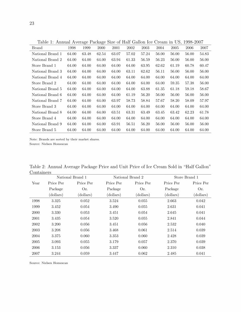
In table 1 we report the annual average package size in the half gallon category for each

major brand.2 At this level of aggregation the transition from 64 oz. to 56 oz. is not

discrete. The gradual replacement of old package sizes could be a result of inventory lags,

as brands replace an old package with the new one in any particular store or market.

Also, the smaller package sizes are not introduced at the same time in all cities, so that

national average size changes gradually. As discussed above, the timing of package size

changes differs across brands. Some brands complete the shift to the smaller package as

early as 2004, while others are slower to move to the smaller package, and still others

maintain the larger package throughout the sample.

”Insert Table 1 about here”

In table 2 we compare average annual package price, price per oz., and package size of the

brands with the three largest national market shares. In the case of national brand 1 a

large drop in average package size in 2002 is accompanied by a decrease in price per

package, however price per oz. increased by 0.2 cents, or approximately 4%. In the case

of national brand 2 a large drop in average package size in 2003 is accompanied by an

increase in the average price per oz. of 0.5 cents, or approximately 10%. Levels and

changes of store brand 1’s package size and pricing appear to differ from the the trends of

national brands 1 and 2. Store brand 1’s prices are lower than those of the national

brands. Also, store brand 1 introduces its smaller package at a later date and appears to

5

raise it’s unit price by less than the national brands.


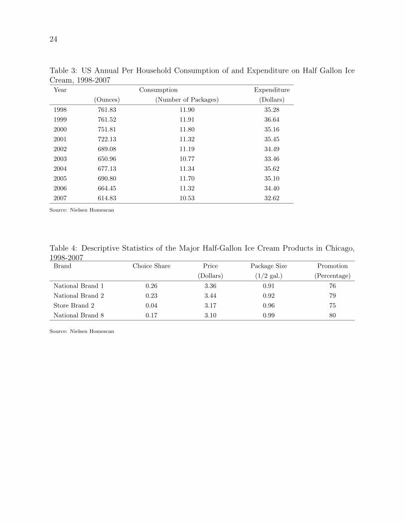
In table 3 we report annual average per-household ice cream consumption in terms of

volume and number of packages, as well as expenditure for half gallon ice cream. Average

household consumption in 1997 was 762 oz., or approximately 12 packages. In 2007,

however, the volume consumption fell by 17% percent to 615 oz. while the number of

packages consumed fell by only 11%. These trends show that on average unit price of half

gallon ice cream has increased proportionately more than its package price, providing

some evidence that downsizing has effectively increased the unit price. Over the same

period we observe annual expenditure on ice cream is relatively stable.


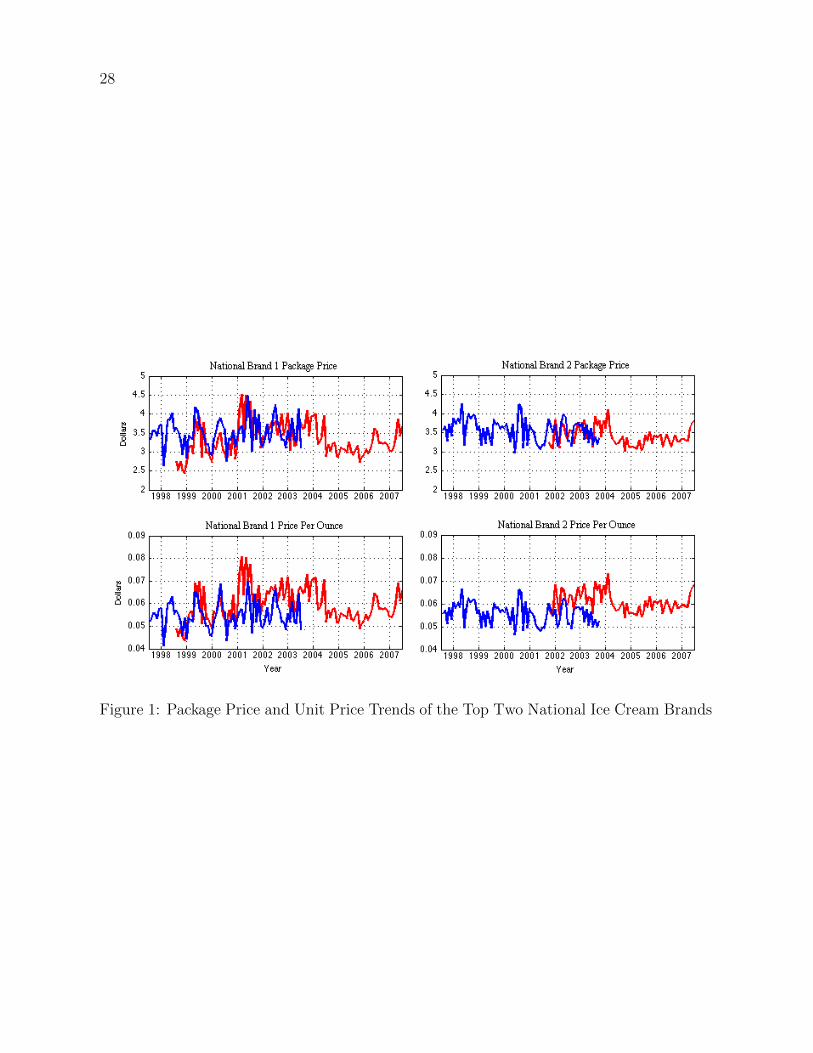
The package size and price trends presented in tables 1 and 2 are averages over all cities.

A narrower focus on one city, Chicago, allows a clearer picture of the interdependencies

between the package size and price of ice cream. Figure 1 presents time series plots of

monthly average ice cream prices of national brand 1 and national brand 2 for each size in

Chicago. The package prices of the 56 oz. products of national brand 1 and 2 appear to

to follow the same trends as their 64 oz. predecessors. However, the smaller packages

appear to have higher unit prices during the transition period. On average, the unit price

of 56 oz. products of both brands are seven percent higher than the unit price of 64 oz.

products. Again, it appears that package downsizing is associated with an increase in the

unit price.

”Insert Figure 1 about here”

6

The data suggest that manufacturers may use downsizing in order to implicitly raise

prices. However, it is not clear at this point that package downsizing is profitable to

manufacturers relative to raising the package price. Answering this question requires a

comparison of the consumer responses to each strategy. In order to capture differential

consumer response to price and package size we now turn to our simultaneous demand

and supply analysis of ice cream markets. In the remainder of the paper we perform our

analysis focusing only on Chicago ice cream market.

ECONOMETRIC MODEL AND BAYESIAN ANALYSIS

We specify a model of demand and supply that explicitly models package size, and

accounts for household heterogeneity and price endogeneity. The econometric model

involves a logistic Normal regression model with random coefficients to represent the

demand function, and a reduced form supply equation to control for endogeneity. To

estimate the model we adopt the Bayesian estimation technique developed by Yang et al.

(2003). We extend the analysis of Yang et al. (2003) in two ways. First, we incorporate an

unbalanced panel in which the choice alternatives are not the same in all periods. Also,

we incorporate household specific demographics in modeling household heterogeneity.

Model

Let i = 1, ..., N , j = 0, ..., J , and t = 1, ..., T denote the index for households, choice

alternatives, and time periods respectively, where j = 0 represents the choice alternative

outside the product category. We observe Nt independent observations in each period, t,

with Jt choice alternatives. The subscript t denotes an unbalanced panel such that the

number of observations and choice alternatives can vary in each period. For each choice

occasion there exists a latent vector Uit(Jt × 1) and the alternative j is observed if the jth

7

component of Uit is larger than all other components. Below we present the formal model.

Uijt = θ′iXjt + ζjt + εijt(1)

pjt = δ′jzjt + ηjt(2)

yijt =

1 if Uijt ≥ max(Uit),

0 otherwise

(3)

Equation 1 specifies the utility of consumer i for brand j in period t in the case that a

purchase is made from J available brands. Consumers have the option of buying an

outside good, j = 0, and obtaining a utility of ui0t = εi0t = 0. The K dimensional vector

Xjt = [xjt pjt] includes the observed product characteristics, xjt, and transaction price,

pjt. Observed product characteristics include package size, promotion and brand-specific

dummies. The K dimensional vector θi includes random coefficients to be estimated. The

unobserved aggregate demand shock ζjt is assumed be common across consumers. The

idiosyncratic shock εijt is assumed to be i.i.d type one Extreme Value (0,1). Equation 2

specifies the reduced form supply equation to control for the endogeneity of prices. The

endogeneity of prices results from the presence of unobserved brand characteristics that

could correlate with prices and influence consumer choices. In this equation, zjt is a Z

vector of instruments that includes average of brand prices in other markets and farm

price of milk, δj is a Z vector of parameters to be estimated, and ηjt is the random supply

shock. It is assumed that the random supply shock, ηt = (η1t, ..., ηJt)′, and the random

demand shock, ζt = (ζ1t, ..., ζJt)′, are correlated but they are independent of the

idiosyncratic shock, εijt:

(4)

ζt

ηt

∼ N

0

0

,

Σ11 Σ12

Σ12 Σ22

≡ N(0,Σ(2J×2J)).

8

Note that in equation 4 if Σ12(J × J) 6= 0, then endogeneity is present. Finally, equation

3 specifies the observed choices of consumer i.

The model is completed with specification of the distribution of consumer heterogeneity.

We assume that the distribution of consumer heterogeneity is multivariate normal with a

mean that is a function of consumer demographics. The heterogeneity is formulated as:

θi = (IK ⊗ di)′Γ + vi

where θi is a K parameter vector of random coefficients, di is a D vector of demographic

variables, Γ is a KD vector of interaction parameters to be estimated, vi ∼ N(0,Σθ),

where Σθ is a K ×K heterogeneity covariance matrix to be estimated.

Under the type one Extreme Value assumption of εijt, the probability of consumer i

choosing product j in period t is given as:

sijt =

(exp(Vijt)

1 +∑J

k=1 exp(Vikt)

).

where Vijt = θ′iXjt + ζjt. Once the choice probabilities are calculated, the predicted shares

of each brand, under the assumptions that the sample is representative and individuals do

not make multiple purchases, is calculated as:

(5) sjt =1

Nt

Nt∑i=1

sijt

Using the predicted shares in equation 5 and the estimated random coefficients the own-

and cross-elasticities of each share with respect to product characteristics, including

9

package size and price, can be calculated as (t is suppressed):

∂sj∂Xj

Xj

sj= 1

N

Xj

sj

∑Ni=1 θisij(1− sij)

∂sj∂Xk

Xk

sj= − 1

NXk

sj

∑Ni=1 θisijsik

We provide the details of Bayesian analysis and estimation in Appendix A and B.

DATA

We use Nielsen Homescan data on half gallon ice cream purchases in Chicago between

1998 and 2007. The data consist of grocery purchases reported by a panel of households.

To participate in the panel a consumer who is 18 or older registers online and provides

demographic information. Based on the consumer demographics Nielsen selects a subset

of consumers to participate in the panel. Participating consumers are provided with a

scanner to record the barcodes of the purchased items and to enter other information,

such as the purchase date and store. The resulting dataset includes information on price

and quantity of products, product characteristics, timing of purchase, promotion

activities, and household characteristics. We conduct our analysis on a subset of

households who record an ice cream purchase in at least 10 of the any 120 months in the

sample. Most of the households that are not included in the data set made only one

purchase, and approximately eighty percent of excluded households made less than six

purchases over the study period.

To estimate our econometric model we match brand level information with household

level information so that in a given month, for a total of 120 months, each household

faces the same brand prices and characteristics. To obtain brand level variables we

aggregate the purchase information on price, package size and promotion in each month

for each brand based on the UPC code. For example, pjt is the average price paid and

sizejt the average package size for brand j in month t, where the average is taken across

10

all purchases of brand j in month t. We construct a promotion variable as the percent of

purchases made with some form of discounting, e.g., coupons or store discounts. For

example, promjt = 75 denotes that 75 percent of households that bought brand j in

period t did so with a discount, while the remaining 25 percent paid the shelf price.

The analysis focuses on four major brands in Chicago: national brand 1, national brand

2, store brand 2 and national brand 83. These brands have the largest shares in Chicago,

and together account for more than 70 percent of the total half gallon ice cream sales

between 1998 and 2007. We observe 609 households in the dataset who on average made

a purchase 24 times during the study period, for a total of 14,522 purchase occasions over

all households.

Table 4 presents descriptive statistics of brand level variables. National brand 1 has the

highest choice share followed by national brand 2. Store brand 2’s choice share is quite

low compared to other brands. National brand 2 has the highest average price and

national brand 8 has the lowest. All of the brands are heavily promoted, with 75 to 80

percent of sales occurring under promotion. We consider 64 oz. as the norm size for half

gallon products, as this was the standard size at the beginning of the study period. We

then express package size as the fraction of the norm size, (Adams et al., 1991) . We note

that national brands 1 and 2 downsized their products early in the study period.

Therefore, the average package size of national brand 1 is the smallest, followed by

national brand 2. Store brand 2 and national brand 8 downsized their products later in

the study period. Also, national brand 8 downsized only a few products among all its half

gallon products, and therefore its average package size is the closest to the norm size. By

2007 only national brand 8 still had 64 oz. products.


We match to the aggregated brand level data with household demographic data,

11

including income, household size, age, education, employment, and race. The information

is available on both female head and male head if the household is not single head. For

these households, we calculate the variables as follows. The education and age variables

are the average of both heads’ education and ages. The income variable is the sum of the

income of both heads. The ethnicity variable reflects the ethnicity of the female head if a

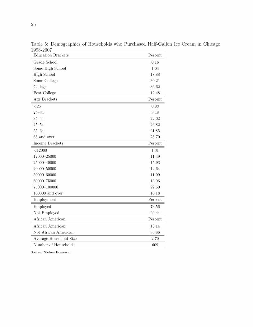
female head is present. Table 5 presents the summary statistics of the demographics of

sample households. The education, age, and income variables are categorical with modes

of college degree, 45-54 years, and $75,000-100,000, respectively. The employment

variable is binary, taking a value of 1 if at least one of the household heads is employed

for more than 35 hours a week. Finally, the household size variable is continuous with an

average of 2.7.


Finally, as instruments for endogenous price we use the average of the prices of each

brand in other markets (Nevo, 2001), as well as the national average farm price of milk,

obtained from USDA.

RESULTS AND DISCUSSION

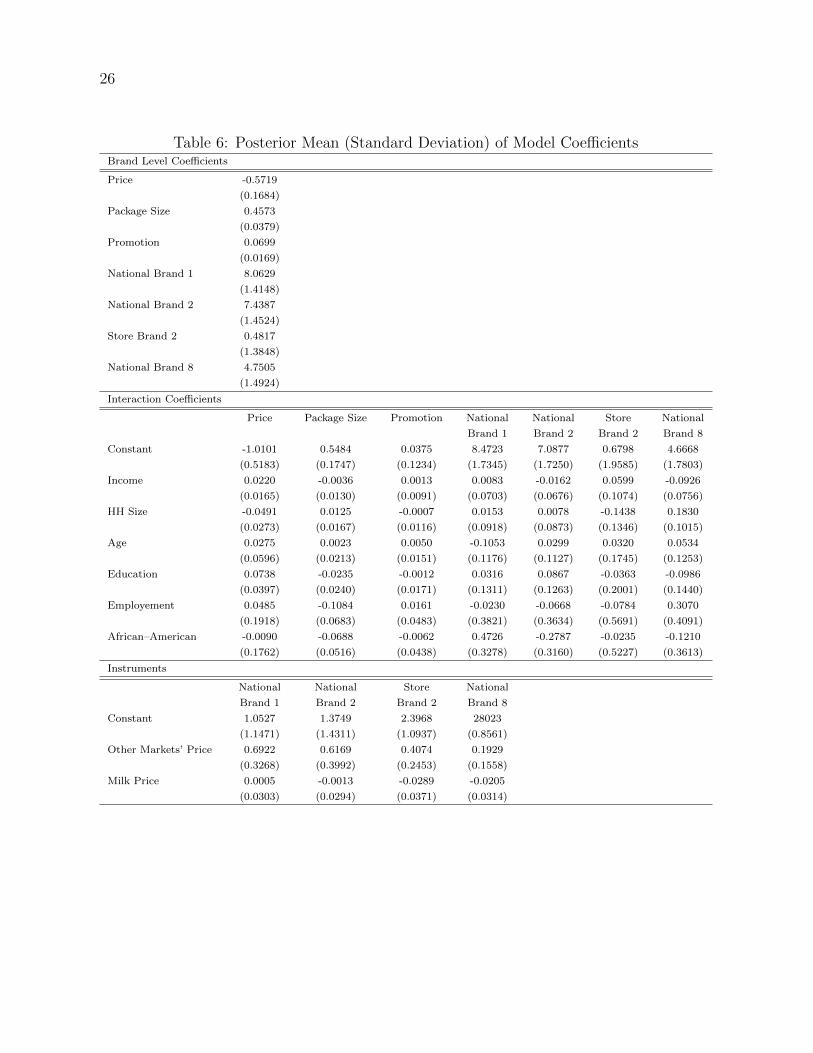
We report the posterior means and posterior standard deviations of the the model

coefficients in table 6. All of the random coefficients have a mass away from zero. The

means of coefficients on package price, package size, and promotion conform with our

expectations. Accordingly, on average an increase in package price decreases the

probability of purchase, whereas an increase in package size or promotion increases the

probability of purchase. The estimates on random coefficients do not have straightforward

economic interpretations; to that end we calculate the elasticity estimates which we

discuss at the end of this section. The estimates of the brand coefficients are consistent

12

with the brand choice shares. National brand 1 has the largest intercept, followed closely

by national brand 2. Store brand 2 has the smallest brand intercept.


Many of the demographics influence consumer sensitivity to price and package size. For

example, income and education have positive effects and household size has a negative

effect on the price coefficient. Thus higher-income households are less price sensitive and

larger households are more price sensitive. Households with higher education attainment

are less price sensitive even controlling for income. Among the demographics influencing

consumer sensitivity to package size, higher income consumers are less sensitive and

larger households more sensitive to changes in package size. And the negative effect of the

education variable suggests that higher educated households are less sensitive to changes

in package size. However, these estimates have a mass around zero. A couple of

demographic effects on the package size coefficient have a mass away from zero. The

employment variable has a negative effect indicating that working households are less

sensitive to package size changes. This result is similar to the finding of Binkley and

Bejnarowicz (2003) that time-constrained consumers substitute a general knowledge of

prices for careful comparisons. In this case, it may be that time-constrained consumers

are less likely to make careful package size comparisons therefore are less sensitive to

downsizing. Also, the results suggest that the African American variable has a negative

effect on the coefficient of package size, again indicating less sensitivity to downsizing.

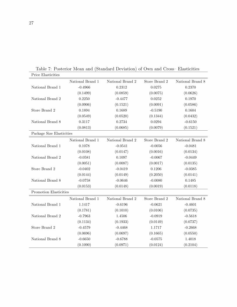
Table 7 reports posterior means and standard deviations of the demand elasticities with

respect to package size and price that are central to the objectives of this study. We find

that the average own-package size elasticity is approximately 0.12 with mass away from

zero, while the the average own-price elasticity is approximately -0.5 with mass away from

zero. Demand for ice cream is price inelastic, as expected. Moreover, consumers are

13

approximately four times more sensitive to package price than package size.


All of the estimates of elasticities have the expected signs and mass away from zero. More

generally, the brand-specific own-price elasticities indicate inelastic demand, and all are

close in magnitude. National brand 1 has the most inelastic own price elasticity with a

value of -0.48, while national brand 8 has the least inelastic own price elasticity with a

value of -0.62. As expected, due to its small market share, the prices of store brand 2

affects the demand for other brands considerably less than the effects of the pricing

strategies of national brands on store brand 2’s demand.

Similarly, ice cream demand is inelastic with respect to own package size, and all the

own-package size elasticities are close in magnitude. Demand for national brand 1 is most

package-size inelastic with a value of 0.11 and demand for national brand 8 is the least

package-size inelastic with a value of 0.15. We also observe a very similar pattern in

relative magnitudes of cross-package size elasticities as in cross-price elasticities. An

interesting finding is that when downsizing occurs consumers switch more heavily to

products with larger package size. For example, elasticity of demand for national brand 8

with respect to national brand 1’s package size is approximately -0.08, where as elasticity

of demand for national brand 2 with respect to national brand 1’s package size is around

-0.06. That is, when national brand 1 downsizes its products consumers switch to

purchase national brand 8 more heavily than national brand 2 products, even though

national brand 2 has a larger market share than national brand 8.

It is important to interpret these elasticities as the average response to downsizing from

64 oz. to 56 oz. products from 1998 to 2007. Consumers’ perceptions of the norm size

and the degree of downsizing can be important factors that effect response to downsizing

14

(Adams et al., 1991). For example, the response to downsizing of a different category (i.e.,

downsizing of 16 oz. ice cream products to 14 oz.) or the response to downsizing from 64

oz. say to 40 oz. can be different. We may not expect a linear relationship between the

package size elasticities and the extend of downsizing. That being recognized, the

estimates provide important insights to manufacturers’ downsizing strategy. In absolute

values the package size elasticities are about a fourth of the own price elasticities.

Therefore, this provides strong evidence that manufacturers have incentives to downsize

as it can enhance price-cost margins compared to equivalent changes in price.

Finally, ice cream demand is elastic with respect to promotion and again all the

own-promotion elasticities are close in magnitude. Demand for national brand 2 is the

most elastic with respect to promotion with a value of 1.45, while demand for national

brand 1 is the least elastic with respect to promotion with a value of 1.14. The pattern of

cross-promotion elasticities are similar to patterns for price and package size elasticities,

with store brand’s promotion affecting the demand for other brands’ ice cream

considerably less than other brands’ promotion affecting the demand for store brand’s ice

cream.

CONCLUSION

Package downsizing is frequently observed in retail U.S. food markets. Food

manufacturers’ incentives to reduce package size hinge on differential consumer response

to changes in price and package size. While mountains of evidence exist on

price-elasticities of food demand, this study is the first to quantify consumer response to

package size. To do so we estimate a market equilibrium model of a differentiated

products market on data from the U.S. market for ice cream.

We specify a random coefficient logit demand equation that explicitly captures consumer

response to changes in package size. We account for the household heterogeneity which

15

we model as a function of household demographics. We address price endogeneity using a

reduced form supply equation. We extend the approach employed by Yang et al. (2003)

by incorporating unbalanced choice alternatives in a Bayesian framework.

A key finding is that that on average consumers are approximately four times as sensitive

to package price as they are to package size; we estimate an elasticity of demand with

respect to package size of 0.12, and a price-elasticity of demand of -0.51. The implication

is that food manufacturers may be able to hide increases in the unit price by

manipulating the package size. To the extent that consumers do respond to package size,

our results indicate that consumers switch more heavily to products with larger package

size. We also find that consumers with more education and higher income are less

sensitive to both prices and package size, and larger households are more sensitive to

price and package size.

16

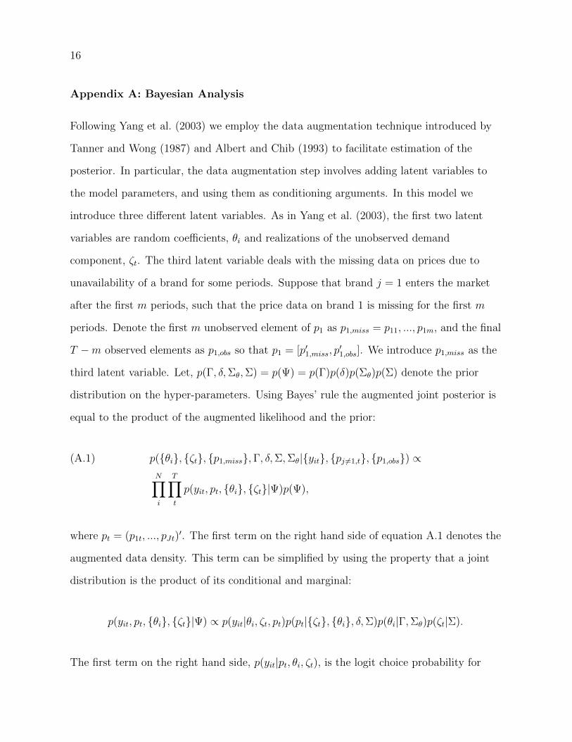
Appendix A: Bayesian Analysis

Following Yang et al. (2003) we employ the data augmentation technique introduced by

Tanner and Wong (1987) and Albert and Chib (1993) to facilitate estimation of the

posterior. In particular, the data augmentation step involves adding latent variables to

the model parameters, and using them as conditioning arguments. In this model we

introduce three different latent variables. As in Yang et al. (2003), the first two latent

variables are random coefficients, θi and realizations of the unobserved demand

component, ζt. The third latent variable deals with the missing data on prices due to

unavailability of a brand for some periods. Suppose that brand j = 1 enters the market

after the first m periods, such that the price data on brand 1 is missing for the first m

periods. Denote the first m unobserved element of p1 as p1,miss = p11, ..., p1m, and the final

T −m observed elements as p1,obs so that p1 = [p′1,miss, p′1,obs]. We introduce p1,miss as the

third latent variable. Let, p(Γ, δ,Σθ,Σ) = p(Ψ) = p(Γ)p(δ)p(Σθ)p(Σ) denote the prior

distribution on the hyper-parameters. Using Bayes’ rule the augmented joint posterior is

equal to the product of the augmented likelihood and the prior:

p({θi}, {ζt}, {p1,miss},Γ, δ,Σ,Σθ|{yit}, {pj 6=1,t}, {p1,obs}) ∝(A.1)

N∏i

T∏t

p(yit, pt, {θi}, {ζt}|Ψ)p(Ψ),

where pt = (p1t, ..., pJt)′. The first term on the right hand side of equation A.1 denotes the

augmented data density. This term can be simplified by using the property that a joint

distribution is the product of its conditional and marginal:

p(yit, pt, {θi}, {ζt}|Ψ) ∝ p(yit|θi, ζt, pt)p(pt|{ζt}, {θi}, δ,Σ)p(θi|Γ,Σθ)p(ζt|Σ).

The first term on the right hand side, p(yit|pt, θi, ζt), is the logit choice probability for

17

consumer i in market t:

p(yit|pt, θi, ζt) =J∏j=1

(exp(Vijt)

1 +∑

k exp(Vikt))

)∀j, k = 1, ..., J

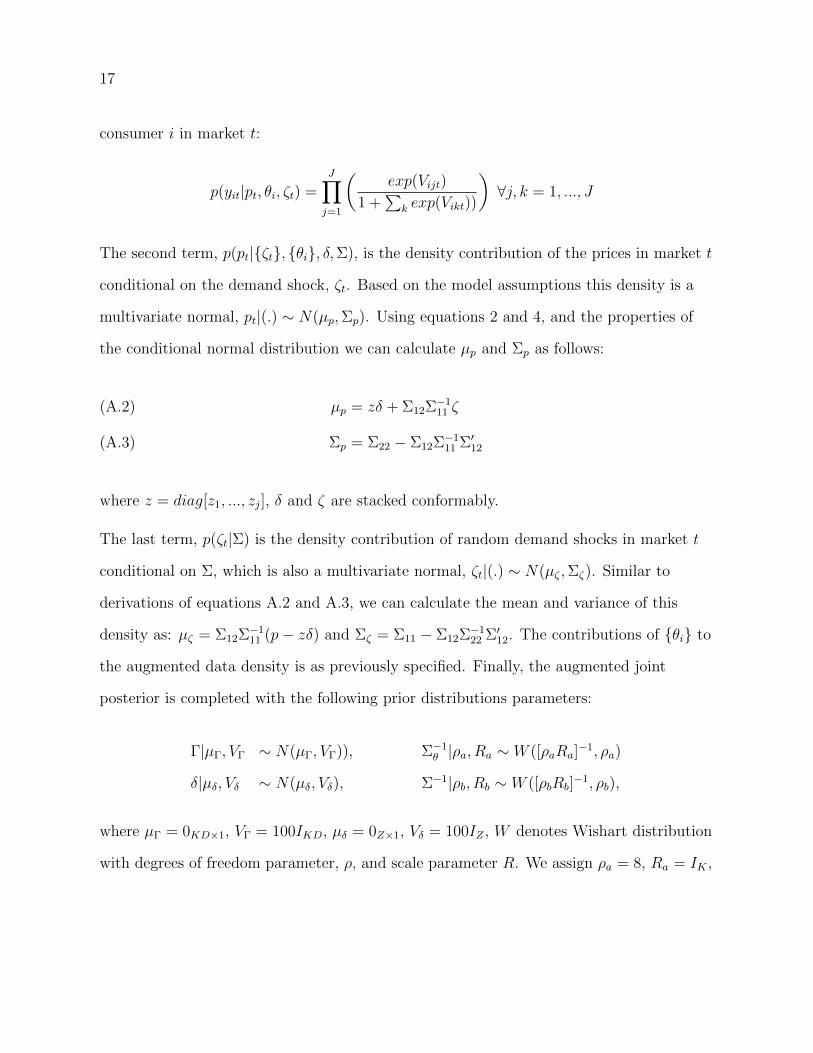
The second term, p(pt|{ζt}, {θi}, δ,Σ), is the density contribution of the prices in market t

conditional on the demand shock, ζt. Based on the model assumptions this density is a

multivariate normal, pt|(.) ∼ N(µp,Σp). Using equations 2 and 4, and the properties of

the conditional normal distribution we can calculate µp and Σp as follows:

µp = zδ + Σ12Σ−111 ζ(A.2)

Σp = Σ22 − Σ12Σ−111 Σ′12(A.3)

where z = diag[z1, ..., zj], δ and ζ are stacked conformably.

The last term, p(ζt|Σ) is the density contribution of random demand shocks in market t

conditional on Σ, which is also a multivariate normal, ζt|(.) ∼ N(µζ ,Σζ). Similar to

derivations of equations A.2 and A.3, we can calculate the mean and variance of this

density as: µζ = Σ12Σ−111 (p− zδ) and Σζ = Σ11 − Σ12Σ−1

22 Σ′12. The contributions of {θi} to

the augmented data density is as previously specified. Finally, the augmented joint

posterior is completed with the following prior distributions parameters:

Γ|µΓ, VΓ ∼ N(µΓ, VΓ)), Σ−1θ |ρa, Ra ∼ W ([ρaRa]

−1, ρa)

δ|µδ, Vδ ∼ N(µδ, Vδ), Σ−1|ρb, Rb ∼ W ([ρbRb]−1, ρb),

where µΓ = 0KD×1, VΓ = 100IKD, µδ = 0Z×1, Vδ = 100IZ , W denotes Wishart distribution

with degrees of freedom parameter, ρ, and scale parameter R. We assign ρa = 8, Ra = IK ,

18

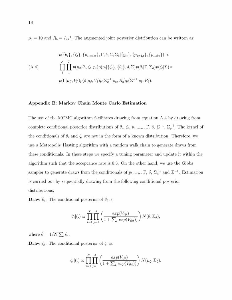
ρb = 10 and Rb = I2J4. The augmented joint posterior distribution can be written as:

p({θi}, {ζt}, {p1,miss},Γ, δ,Σ,Σθ|{yit}, {pj 6=1,t}, {p1,obs}) ∝N∏i

T∏t

p(yit|θi, ζt, pt)p(pt|{ζt}, {θi}, δ,Σ)p(θi|Γ,Σθ)p(ζt|Σ)×(A.4)

p(Γ|µΓ, VΓ)p(δ|µδ, Vδ)p(Σ−1θ |ρa, Ra)p(Σ

−1|ρb, Rb).

Appendix B: Markov Chain Monte Carlo Estimation

The use of the MCMC algorithm facilitates drawing from equation A.4 by drawing from

complete conditional posterior distributions of θi, ζt, p1,miss, Γ, δ, Σ−1, Σ−1θ . The kernel of

the conditionals of θi and ζt are not in the form of a known distribution. Therefore, we

use a Metropolis–Hasting algorithm with a random walk chain to generate draws from

these conditionals. In these steps we specify a tuning parameter and update it within the

algorithm such that the acceptance rate is 0.3. On the other hand, we use the Gibbs

sampler to generate draws from the conditionals of p1,miss, Γ, δ, Σ−1θ and Σ−1. Estimation

is carried out by sequentially drawing from the following conditional posterior

distributions:

Draw θi: The conditional posterior of θi is:

θi|(.) ∝T∏t=1

J∏j=1

(exp(Vijt)

1 +∑

k exp(Vikt))

)N(θ̄,Σθ),

where θ̄ = 1/N∑

i θi.

Draw ζt: The conditional posterior of ζt is:

ζt|(.) ∝N∏i=1

J∏j=1

(exp(Vijt)

1 +∑

k exp(Vikt))

)N(µζ ,Σζ).

19

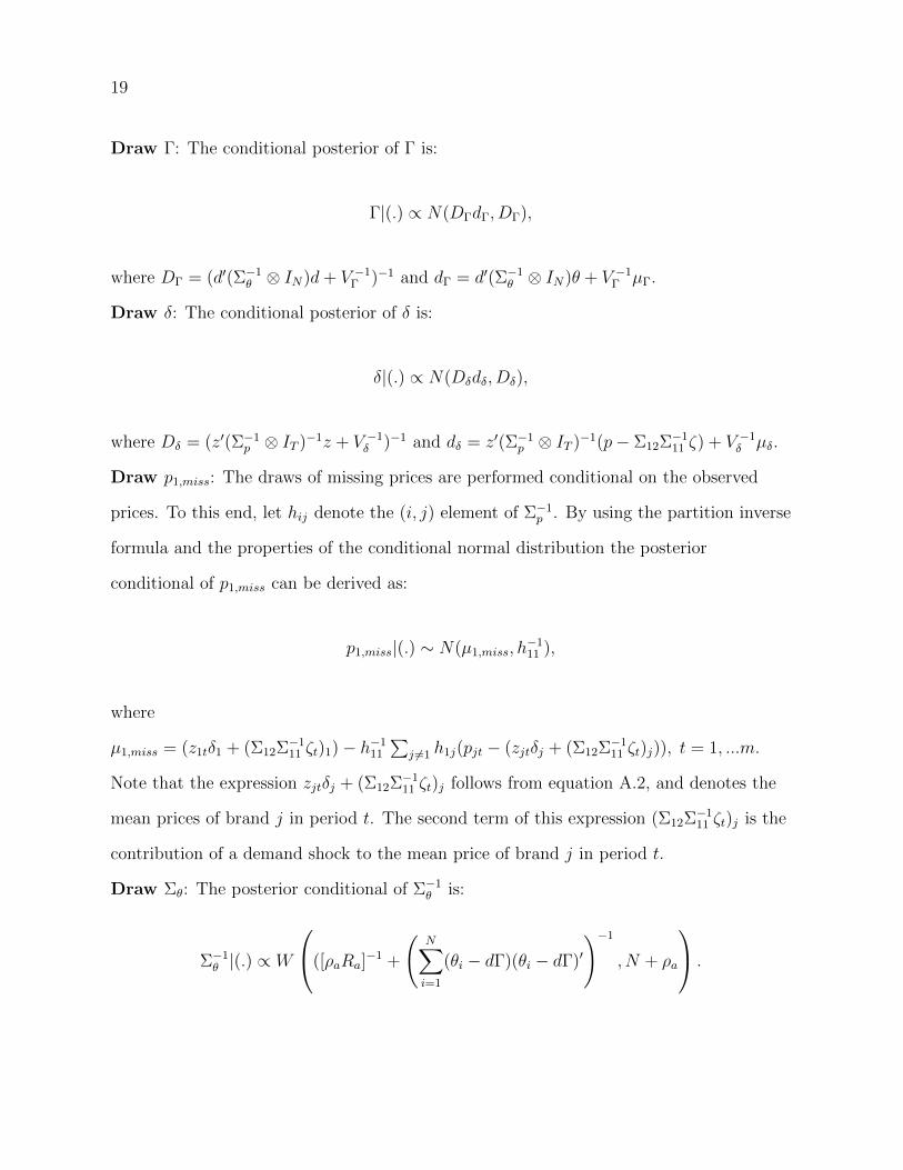
Draw Γ: The conditional posterior of Γ is:

Γ|(.) ∝ N(DΓdΓ, DΓ),

where DΓ = (d′(Σ−1θ ⊗ IN)d+ V −1

Γ )−1 and dΓ = d′(Σ−1θ ⊗ IN)θ + V −1

Γ µΓ.

Draw δ: The conditional posterior of δ is:

δ|(.) ∝ N(Dδdδ, Dδ),

where Dδ = (z′(Σ−1p ⊗ IT )−1z + V −1

δ )−1 and dδ = z′(Σ−1p ⊗ IT )−1(p− Σ12Σ−1

11 ζ) + V −1δ µδ.

Draw p1,miss: The draws of missing prices are performed conditional on the observed

prices. To this end, let hij denote the (i, j) element of Σ−1p . By using the partition inverse

formula and the properties of the conditional normal distribution the posterior

conditional of p1,miss can be derived as:

p1,miss|(.) ∼ N(µ1,miss, h−111 ),

where

µ1,miss = (z1tδ1 + (Σ12Σ−111 ζt)1)− h−1

11

∑j 6=1 h1j(pjt − (zjtδj + (Σ12Σ−1

11 ζt)j)), t = 1, ...m.

Note that the expression zjtδj + (Σ12Σ−111 ζt)j follows from equation A.2, and denotes the

mean prices of brand j in period t. The second term of this expression (Σ12Σ−111 ζt)j is the

contribution of a demand shock to the mean price of brand j in period t.

Draw Σθ: The posterior conditional of Σ−1θ is:

Σ−1θ |(.) ∝ W

([ρaRa]−1 +

(N∑i=1

(θi − dΓ)(θi − dΓ)′

)−1

, N + ρa

.

20

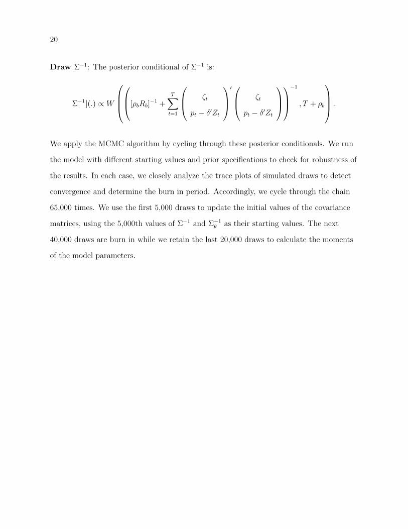
Draw Σ−1: The posterior conditional of Σ−1 is:

Σ−1|(.) ∝ W

[ρbRb]

−1 +T∑t=1

ζt

pt − δ′Zt

′ ζt

pt − δ′Zt

−1

, T + ρb

.

We apply the MCMC algorithm by cycling through these posterior conditionals. We run

the model with different starting values and prior specifications to check for robustness of

the results. In each case, we closely analyze the trace plots of simulated draws to detect

convergence and determine the burn in period. Accordingly, we cycle through the chain

65,000 times. We use the first 5,000 draws to update the initial values of the covariance

matrices, using the 5,000th values of Σ−1 and Σ−1θ as their starting values. The next

40,000 draws are burn in while we retain the last 20,000 draws to calculate the moments

of the model parameters.

21

REFERENCES

Adams, C. et al. (1991). Can you reduce your package size without damaging sales? Long

Range Planning 24 (4), 86–96.

Albert, J. and S. Chib (1993). Bayesian analysis of binary and polychotomous response

data. Journal of the American Statistical Association 88 (422), 669–679.

Binkley, J. and J. Bejnarowicz (2003). Consumer price awareness in food shopping: the

case of quantity surcharges. Journal of Retailing 79 (1), 27–35.

Granger, C. and A. Billson (1972). Consumers’ attitudes toward package size and price.

Journal of Marketing Research 9 (3), 239–248.

Lennard, D., V. Mitchell, P. McGoldrick, and E. Betts (2001). Why consumers under-use

food quantity indicators. The International Review of Retail, Distribution and

Consumer Research 11 (2), 177–199.

Nevo, A. (2001). Measuring market power in the ready-to-eat cereal market.

Econometrica 69 (2), 307–342.

Russo, J. (1977). The value of unit price information. Journal of Marketing

Research 14 (2), 193–201.

Tanner, M. and W. Wong (1987). The calculation of posterior distributions by data

augmentation. Journal of the American statistical Association 82 (398), 528–540.

Wansink, B. (1996). Can package size accelerate usage volume? The Journal of

Marketing 60 (3), 1–14.

Yang, S., Y. Chen, and G. Allenby (2003). Bayesian analysis of simultaneous demand and

supply. Quantitative Marketing and Economics 1 (3), 251–275.

22

Notes

1Throughout the paper we use ”half gallon” to refer to both 64 and 56 oz. products.

2Brands with at least 1.5% share of national market volume.

3We observe purchases of store brand 2 after the first 16 months of the study period.

4Estimation results are robust to alternative diffuse assignments of hyper-parameters, such as VΓ =

10IKD or VΓ = 1000IKD, Vδ = 10IZ or Vδ = 1000IZ , ρa = 10 or ρa = 14, Ra = 0.5IK or Ra = 2IK ,

ρb = 12 or ρb = 16 and Rb = 0.5I2J or Rb = 2I2J .

23

Table 1: Annual Average Package Size of Half Gallon Ice Cream in US, 1998-2007Brand 1998 1999 2000 2001 2002 2003 2004 2005 2006 2007

National Brand 1 64.00 63.48 62.54 63.07 57.02 57.24 56.00 56.00 56.00 54.83

National Brand 2 64.00 64.00 64.00 63.94 61.33 56.59 56.23 56.00 56.00 56.00

Store Brand 1 64.00 64.00 64.00 64.00 64.00 63.95 62.62 61.19 60.78 60.47

National Brand 3 64.00 64.00 64.00 64.00 63.11 62.62 56.11 56.00 56.00 56.00

National Brand 4 64.00 64.00 64.00 64.00 64.00 64.00 64.00 64.00 64.00 64.00

Store Brand 2 64.00 64.00 64.00 64.00 64.00 64.00 64.00 59.35 57.38 56.00

National Brand 5 64.00 64.00 64.00 64.00 64.00 63.88 61.35 61.18 59.18 58.67

National Brand 6 64.00 64.00 64.00 64.00 61.19 56.20 56.00 56.00 56.00 56.00

National Brand 7 64.00 64.00 64.00 63.97 58.73 58.84 57.67 58.20 58.09 57.97

Store Brand 3 64.00 64.00 64.00 64.00 64.00 64.00 64.00 64.00 64.00 64.00

National Brand 8 64.00 64.00 64.00 63.51 63.31 63.49 63.45 63.42 62.23 61.78

Store Brand 4 64.00 64.00 64.00 64.00 64.00 64.00 64.00 64.00 64.00 64.00

National Brand 9 64.00 64.00 64.00 63.91 56.51 56.20 56.00 56.00 56.00 56.00

Store Brand 5 64.00 64.00 64.00 64.00 64.00 64.00 64.00 64.00 64.00 64.00

Note: Brands are sorted by their market shares.

Source: Nielsen Homescan

Table 2: Annual Average Package Price and Unit Price of Ice Cream Sold in “Half Gallon”Containers

National Brand 1 National Brand 2 Store Brand 1

Year Price Per Price Per Price Per Price Per Price Per Price Per

Package Oz. Package Oz. Package Oz.

(dollars) (dollars) (dollars) (dollars) (dollars) (dollars)

1998 3.325 0.052 3.524 0.055 2.663 0.042

1999 3.452 0.054 3.490 0.055 2.631 0.041

2000 3.330 0.053 3.451 0.054 2.645 0.041

2001 3.435 0.054 3.520 0.055 2.841 0.044

2002 3.200 0.056 3.451 0.056 2.532 0.040

2003 3.208 0.056 3.468 0.061 2.514 0.039

2004 3.375 0.060 3.353 0.060 2.428 0.039

2005 3.093 0.055 3.179 0.057 2.370 0.039

2006 3.153 0.056 3.337 0.060 2.310 0.038

2007 3.244 0.059 3.447 0.062 2.485 0.041


24

Table 3: US Annual Per Household Consumption of and Expenditure on Half Gallon IceCream, 1998-2007

Year Consumption Expenditure

(Ounces) (Number of Packages) (Dollars)

1998 761.83 11.90 35.28

1999 761.52 11.91 36.64

2000 751.81 11.80 35.16

2001 722.13 11.32 35.45

2002 689.08 11.19 34.49

2003 650.96 10.77 33.46

2004 677.13 11.34 35.62

2005 690.80 11.70 35.10

2006 664.45 11.32 34.40

2007 614.83 10.53 32.62


Table 4: Descriptive Statistics of the Major Half-Gallon Ice Cream Products in Chicago,1998-2007

Brand Choice Share Price Package Size Promotion

(Dollars) (1/2 gal.) (Percentage)

National Brand 1 0.26 3.36 0.91 76

National Brand 2 0.23 3.44 0.92 79

Store Brand 2 0.04 3.17 0.96 75

National Brand 8 0.17 3.10 0.99 80


25

Table 5: Demographics of Households who Purchased Half-Gallon Ice Cream in Chicago,1998-2007

Education Brackets Percent

Grade School 0.16

Some High School 1.64

High School 18.88

Some College 30.21

College 36.62

Post College 12.48

Age Brackets Percent

<25 0.83

25–34 3.48

35–44 22.02

45–54 26.82

55–64 21.85

65 and over 25.70

Income Brackets Percent

<12000 1.31

12000–25000 11.49

25000–40000 15.93

40000–50000 12.64

50000–60000 11.99

60000–75000 13.96

75000–100000 22.50

100000 and over 10.18

Employment Percent

Employed 73.56

Not Employed 26.44

African American Percent

African American 13.14

Not African American 86.86

Average Household Size 2.70

Number of Households 609


26

Table 6: Posterior Mean (Standard Deviation) of Model CoefficientsBrand Level Coefficients

Price -0.5719

(0.1684)

Package Size 0.4573

(0.0379)

Promotion 0.0699

(0.0169)

National Brand 1 8.0629

(1.4148)


(1.4524)

Store Brand 2 0.4817

(1.3848)


(1.4924)

Interaction Coefficients

Price Package Size Promotion National National Store National

Brand 1 Brand 2 Brand 2 Brand 8

Constant -1.0101 0.5484 0.0375 8.4723 7.0877 0.6798 4.6668

(0.5183) (0.1747) (0.1234) (1.7345) (1.7250) (1.9585) (1.7803)

Income 0.0220 -0.0036 0.0013 0.0083 -0.0162 0.0599 -0.0926

(0.0165) (0.0130) (0.0091) (0.0703) (0.0676) (0.1074) (0.0756)

HH Size -0.0491 0.0125 -0.0007 0.0153 0.0078 -0.1438 0.1830

(0.0273) (0.0167) (0.0116) (0.0918) (0.0873) (0.1346) (0.1015)

Age 0.0275 0.0023 0.0050 -0.1053 0.0299 0.0320 0.0534

(0.0596) (0.0213) (0.0151) (0.1176) (0.1127) (0.1745) (0.1253)

Education 0.0738 -0.0235 -0.0012 0.0316 0.0867 -0.0363 -0.0986

(0.0397) (0.0240) (0.0171) (0.1311) (0.1263) (0.2001) (0.1440)

Employement 0.0485 -0.1084 0.0161 -0.0230 -0.0668 -0.0784 0.3070

(0.1918) (0.0683) (0.0483) (0.3821) (0.3634) (0.5691) (0.4091)

African–American -0.0090 -0.0688 -0.0062 0.4726 -0.2787 -0.0235 -0.1210

(0.1762) (0.0516) (0.0438) (0.3278) (0.3160) (0.5227) (0.3613)

Instruments

National National Store National

Brand 1 Brand 2 Brand 2 Brand 8

Constant 1.0527 1.3749 2.3968 28023

(1.1471) (1.4311) (1.0937) (0.8561)

Other Markets’ Price 0.6922 0.6169 0.4074 0.1929

(0.3268) (0.3992) (0.2453) (0.1558)

Milk Price 0.0005 -0.0013 -0.0289 -0.0205

(0.0303) (0.0294) (0.0371) (0.0314)

27

Table 7: Posterior Mean and (Standard Deviation) of Own and Cross– ElasticitiesPrice Elasticities

National Brand 1 National Brand 2 Store Brand 2 National Brand 8

National Brand 1 -0.4966 0.2312 0.0275 0.2370

(0.1499) (0.0859) (0.0075) (0.0626)

National Brand 2 0.2250 -0.4477 0.0252 0.1970

(0.0906) (0.1521) (0.0091) (0.0586)

Store Brand 2 0.1894 0.1689 -0.5190 0.1604

(0.0549) (0.0520) (0.1344) (0.0432)

National Brand 8 0.3117 0.2734 0.0294 -0.6150

(0.0813) (0.0685) (0.0079) (0.1521)

Package Size Elasticities


National Brand 1 0.1078 -0.0541 -0.0056 -0.0481

(0.0108) (0.0147) (0.0016) (0.0134)

National Brand 2 -0.0581 0.1097 -0.0067 -0.0449

(0.0051) (0.0087) (0.0017) (0.0135)

Store Brand 2 -0.0402 -0.0419 0.1206 -0.0385

(0.0144) (0.0149) (0.2050) (0.0141)

National Brand 8 -0.0758 -0.0646 -0.0080 0.1485

(0.0153) (0.0148) (0.0019) (0.0118)

Promotion Elasticities


National Brand 1 1.1417 -0.6196 -0.0621 -0.4601

(0.1781) (0.1010) (0.0106) (0.0735)

National Brand 2 -0.7963 1.4506 -0.0919 -0.5618

(0.1134) (0.1933) (0.0149) (0.0737)

Store Brand 2 -0.4579 -0.4468 1.1717 -0.2668

(0.0696) (0.0697) (0.1665) (0.0550)

National Brand 8 -0.6650 -0.6788 -0.0575 1.4018

(0.1090) (0.0971) (0.0124) (0.2104)

28

Figure 1: Package Price and Unit Price Trends of the Top Two National Ice Cream Brands

Documents

Estimating Consumer Response to Package Downsizing… · Estimating Consumer Response to Package Downsizing: an Application to Chicago Ice Cream Market Abstract We estimate a random