Estimating Average and Local Average Treatment …faculty.smu.edu/millimet/classes/eco7321/papers/...change. The break in education attainment is so stark in both Britain and Northern

Estimating Average and Local Average Treatment Effects ofEducation when Compulsory Schooling Laws Really Matter

By PHILIP OREOPOULOS*

The change to the minimum school-leaving age in the United Kingdom from 14 to15 had a powerful and immediate effect that redirected almost half the populationof 14-year-olds in the mid-twentieth century to stay in school for one more year. Themagnitude of this impact provides a rare opportunity to (a) estimate local averagetreatment effects (LATE) of high school that come close to population averagetreatment effects (ATE); and (b) estimate returns to education using a regressiondiscontinuity design instead of previous estimates that rely on difference-in-differencesmethodology or relatively weak instruments. Comparing LATE estimates for theUnited States and Canada, where very few students were affected by compulsoryschool laws, to the United Kingdom estimates provides a test as to whetherinstrumental variables (IV) returns to schooling often exceed ordinary least squares(OLS) because gains are high only for small and peculiar groups among the moregeneral population. I find, instead, that the benefits from compulsory schooling arevery large whether these laws have an impact on a majority or minority of thoseexposed. (JEL I20, I21, I28)

Researchers routinely use the IV method toevaluate programs and estimate consistent treat-ment effects. A valid instrumental variable,which helps determine whether an individual istreated, but does not determine other factors thataffect the outcomes of interest, can overcomeestimation biases that often arise when using theOLS method. Recent work in this field clarifies

how to interpret estimated treatment effects us-ing IV. When the treatment being evaluated hasthe same effect for everyone, any valid instru-ment will identify this unique parameter. Butwhen responses to treatment vary, different in-struments measure different effects. Guido W.Imbens and Joshua D. Angrist (1994) point outthat, in this more realistic environment, the onlyeffect we can be sure that this method estimatesis the average treatment effect among those whoalter their treatment status because they react tothe instrument; they call this parameter theLATE. In some cases, the LATE also equals theaverage treatment effect among those exposedto the treatment, but only when persons do notmake decisions to react to the instrument basedon factors that also determine treatment gains(James J. Heckman, 1997).

In the return to schooling literature, research-ers frequently use IV. Some often-cited exam-ples include studies that measure the LATEamong persons who attend college because theylive close to college (David Card, 1995); per-sons who attend college because tuition is low(Thomas J. Kane and Cecilia Elena Rouse,1995) and persons obliged to stay in schoollonger because they face more restrictive com-

* Department of Economics, University of Toronto, 140St. George Street, Toronto M55 3G6, Canada, and NationalBureau of Economic Research (e-mail: [email protected]). I am very grateful to Joshua Angrist, EnricoMoretti, and staff members from the U.K. Data Archive forproviding me with necessary data for this project. Seminarand conference participants at UC-Berkeley, the LondonSchool of Economics, the Chicago Federal Reserve, RoyalHolloway, Duke University, McGill University, QueensUniversity, NBER Summer Institute, IZA/SOLE Transat-lantic Meetings, and the universities of Toronto, BritishColumbia, and Guelph provided helpful discussion. I amespecially thankful to George Akerlof, Joshua Angrist, AlanAuerbach, David Autor, Michael Baker, Gregory Besharov,David Card, Liz Cascio, Stacey Chen, Botond Koszegi,John Quigley, Marco Manacorda, Rob McMillan, JustinMcCrary, Costas Meghir, Mathew Rabin, Jesse Rothstein,Emmanuel Saez, Aloysius Siow, Alois Stutzer, Jo VanBiesebroeck, Ian Walker, and three anonymous referees formany helpful comments and discussions. I am solely re-sponsible for this paper’s contents.

152

pulsory school laws (Angrist and Alan B.Krueger, 1991; Daron Acemoglu and Angrist,2001). These instruments typically affect fewerthan 10 percent of the population exposed to theinstrument and often generate treatment effectsthat exceed those generated from OLS. Card(2001) and Lang (1993) suggest that the higherIV results could occur because they approxi-mate average effects among a small and pecu-liar group, whereas OLS estimates, in theabsence of omitted variables and measurementerror biases, approximate average effectsamong everyone. In a model where individualsweigh costs and benefits from attaining addi-tional school, LATE estimates from IV couldexceed OLS estimates for a variety of reasons,for example, because individuals affected by theinstruments are more credit constrained, havegreater immediate need to work, or have greaterdistaste for school.1

Previous LATE estimates have provided littleinkling about what the gains to schooling are fora more general population. An alternative pa-rameter that captures this is the ATE, theexpected gain from schooling among all indi-viduals (or all individuals with a given set ofcovariates). Unlike the LATE, it does not de-pend on a particular instrument or on who getstreated. The ATE offers a theoretically morestable parameter when considering potential gainsfor anyone receiving an extra year of schooling orcollege study. A comparison between ATE andprevious LATE estimates would help determinewhether the earlier LATE results are anomalies, orwhether the effects of education are by and largesimilar across a wider population.

In this paper, I exploit historically high drop-out rates in the United Kingdom to estimate theLATE for secondary schooling. The result is anIV estimate that is probably closer to the ATEthan any previously reported. I focus on a pe-riod when legislative changes had a remarkableeffect on overall education attainment. Fig-ure 1 shows this effect on the fraction of British-born adults that left full-time education at ages14 or less and 15 or less. It is not difficult to

realize at a glance of the figure that the mini-mum school-leaving age in Britain increasedfrom 14 to 15 in 1947. Within two years of thispolicy change, the portion of 14-year-olds leav-ing school fell from 57 percent to less than 10percent. The trend for the fraction of childrendropping out at age 15 or less, however, re-mained intact—it appears virtually everyonewho would have left school at age 14 left at age15 after the change. I found an equally dramaticresponse to an increase in the minimum legalschool-leaving age in Northern Ireland (see Figure2), where the law change occurred ten years later.

I use these two U.K. experiences to make twocontributions to the returns-to-schooling litera-ture. First, I estimate average returns to highschool from instrumental variables that affectalmost half the population. The magnitude ofthe response from these policies provides a testto whether previous IV estimates often match orexceed OLS estimates because they identifyaverage returns to schooling for a select groupin the population. I demonstrate this test bycomparing the results with LATE estimatesfrom compulsory schooling laws in the UnitedStates and Canada, where very few students leftearly, to the U.K. estimates. If high school drop-outs have more to gain than high school grad-uates from staying on an extra year, the localaverage treatment effect of compulsory educa-tion will be higher than the average treatmenteffect for the total population.2 As the fractionaffected by compulsory education increases, how-ever, the LATE and ATE converge since the ATEincludes the population of would-be dropouts.When the fraction affected by compulsory school-ing increases, we can use the gradient of theseestimates to determine the ATE population. Thisapproach is similar in spirit to one proposed byHeckman and Edward Vytlacil (2001).

My second contribution is to adopt a regres-sion discontinuity (RD) design to estimate av-erage returns to schooling. The RD approachdiffers from previous studies by comparing ed-ucation attainment and adult earnings for stu-dents just prior to and just after the policy

1 Alternatively, IV results might exceed OLS if the in-struments are invalid. Pedro Carneiro and James J. Heck-man (2002) criticize the validity of some earlier studies bydemonstrating that some often-used instruments correlatewith proxies for innate ability.

2 The term “dropout” is something of a misnomer in theUnited Kingdom, since those who failed to advance tosecondary school were expected to leave at the earliestopportunity. I shall occasionally refer to U.K. school leaversas dropouts for convenience.

153VOL. 96 NO. 1 OREOPOULOS: ESTIMATING ATE AND LATE WITH COMPULSORY SCHOOLING LAWS

change. The break in education attainment is sostark in both Britain and Northern Ireland thatwe can show graphically the correspondingbreak in earnings and the source of the LATEidentification.

My analysis addresses some previous con-cerns that have been expressed in the literatureabout the validity of earlier approaches to esti-mate returns to compulsory schooling. One ap-proach, introduced by Angrist and Krueger(1991) uses quarter of birth to identify studentsallowed to drop out with less education thanothers because they were born after the school-entry cutoff date and waited a full year beforeentering school, compared to those born prior tothe cutoff date. John Bound et al. (1995) showthat if education attainment and quarter of birthare only weakly correlated, estimates can bebiased in the same direction as OLS results arebiased.3 A second concern is that timing of birth

may be related to other factors affecting earn-ings. Carneiro and Heckman (2002) providesome evidence that day of birth also relates toproxies for early childhood development.

Another approach takes advantage of differ-ences in the timing of compulsory schoolinglaw changes across regions (e.g., Acemoglu andAngrist, 2001; Lance Lochner and Enrico Mor-etti, 2004; Adriana Lleras-Muney, 2005). Thistechnique uses the same identification strategyas a differences-in-differences research design.To estimate consistently the LATE of compul-sory schooling, the timing of the law changesmust not be correlated with any other policychanges or regional characteristics that also re-late to the outcome variables. These studiesassume, in the absence of law changes, thatrelative trends in the outcome variables are thesame across regions.

3 Douglas Staiger and James H. Stock (1997) and LuizM. Cruz and Marcelo J. Moreira (2005) address concernsabout this source of bias. Both attempt to correct for the

weak instrument bias that may result from using quarter ofbirth to estimate returns to compulsory schooling and arriveat generally similar estimates to Angrist and Kureger’soriginal study.

FIGURE 1. FRACTION LEFT FULL-TIME EDUCATION BY YEAR AGED 14 AND 15(Great Britain)

Note: The lower line shows the proportion of British-born adults aged 32 to 64 from the 1983to 1998 General Household Surveys who report leaving full-time education at or before age14 from 1935 to 1965. The upper line shows the same, but for age 15. The minimum school-leaving age in Great Britain changed in 1947 from 14 to 15.

154 THE AMERICAN ECONOMIC REVIEW MARCH 2006

A third approach also uses changes to theschool-leaving age in the United Kingdom.Colm Harmon and Ian Walker (1995) werethe first to adopt these school-leaving agechanges to estimate returns to schooling, butdid not include birth cohort effects in theirregressions to account for a rising trend ineducation attainment and earnings. As a re-sult, their estimates do not allow for sys-tematic inter-cohort changes in educationalattainment, and do not identify effects fromcohorts who attended school just before andjust after the law changes.

The regression discontinuity method usedin this paper offers more compelling evidenceon the average treatment effects of highschool. The main conclusion of the paper isthat the effects from compulsory schooling,are very large—ranging from an annual gainin earnings between 10 to 14 percent—whether a majority or minority of the popu-lation is affected. I also identify significantgains to health, employment, and other labor

market outcomes. The results provide evi-dence that IV LATE estimates may often besimilar to ATE, and that the main reasonswhy OLS results are weaker than IV are notlikely due to differences in the population ofindividuals affected by the instrument.

The next section outlines a theoreticalframework for interpreting returns to compul-sory schooling and provides a parametric ex-ample of how increasing the fraction affectedby compulsory schooling affects the LATEestimate relative to ATE. Section II providesbackground to the school-leaving age in-creases in Britain and in Northern Ireland.The regression discontinuity and instrumentalvariables analysis is also carried out in Sec-tion II. Section III compares the RD-IV re-sults from Britain and Northern Ireland to theIV results for Canada and the United States.Section IV concludes with a discussion aboutwhy compulsory school laws seem to gener-ate large gains for individuals who otherwisewould have lefts school earlier.

FIGURE 2. FRACTION LEFT FULL-TIME EDUCATION BY YEAR AGED 14 AND 15(Northern Ireland)

Note: The lower line shows the proportion of Northern Irish adults aged 32 to 64 from the1985 to 1998 General Household Surveys who report leaving full-time education at or beforeage 14 from 1935 to 1965. The upper line shows the same, but for age 15. The minimumschool-leaving age in Northern Ireland changed in 1957 from 14 to 15.


I. Theoretical Framework

A. Causal Inference and CompulsorySchooling

In this section, I discuss the theoretical back-ground to my analysis, beginning with howcompulsory-schooling laws facilitate makingcausal inferences about various effects of edu-cation. I illustrate the differences between theLATE and ATE using a parametric example,then discuss the optimal schooling within thecontext of the setup, if schooling is seen as aninvestment. I follow the theoretical frameworkused by Angrist and Krueger (1999) and byAngrist (2004) to link the LATE identified us-ing compulsory schooling as an instrument withthe population ATE.

Let Si be an indicator for whether child iattends school at age 15 (Si � 1) or leaves at age14 (Si � 0). I define schooling, thus, as a binaryvariable indicating only a measure of highschool attainment because this approach bestrepresents the level of attainment affected byraising the minimum school-leaving age.4 LetY1i be child i’s circumstances after age 15 ifSi � 1, and let Y0i be her circumstances after age15 if Si � 0. Although only one of these poten-tial outcomes is ever observed, the averagetreatment effect, E(Y1i � Y0i), can be used tomake predictive statements about the impact ofhigh school on a randomly chosen person.

Let Zi be a binary variable with Zi � 1 if theschool-leaving age equals 15, and Zi � 0 if itequals 14. Suppose Si is determined by thelatent-index assignment mechanism,

(1) Si � 1��0 � �1 Zi � �i �

where �1 � 0 and �i is a random variableindependent of the instrument. The potentialtreatment assignments are S0i � 1(�0 � �i) andS1i � 1(�0 � �1 � �i). The instrument has noeffect on those already intending to attendschool at age 15, but has a nonnegative effect onschooling for those leaving at age 14 without

the law, so that S1i � S0i. Imbens and Angrist(1994) show that this monotonicity assumption,together with independence, implies:

(2)E�Yi�Zi � 1� � E�Yi�Zi � 0�

E�Si�Zi � 1� � E�Si�Zi � 0�

� E�Y1i � Y0i�S1i � S0i�.

The left-hand side of this expression is the pop-ulation analog of the Wald Estimator. SinceS1i � S0i holds only for individuals who leave atage 14 in the absence of the more restrictivelaw, the LATE on the right-hand side is theaverage effect of an additional year of schoolamong those who otherwise would not havetaken that extra year.

B. A Parametric Example

Following Angrist (2004), I calculate a para-metric model to show the relative differencesbetween LATE and ATE using the compulsory-school-law instrument. First, I assume that thedistribution of (Y1i � Y0i , �i) is bivariate nor-mal: (Y1i � Y0i , �i) � N2[�, ��,

2, �2, �].

Thus, the ATE [E(Y1i � Y0i)] is �, the mean of�i is ��, the correlation between Y1i � Y0i and�i is �, and the respective variances for Y1i �Y0i and �i are

2 and �2. If � is positive, the

likelihood of dropping out at age 14 is corre-lated with higher gains from school (after age15). Since everyone must attend school at age15 when the school-leaving age is 15 (�13 �),the LATE is equal to the treatment effect on thenontreated—the average effect of attendingschool at age 15 for those who leave at age 14.It can be written as:

(3)

E�13�

�Y1i � Y0i�S1i � S0i� � E�Y1i � Y0i�S0i � 0�

� E�Y1i � Y0i��i � �0 �

� E�Y1i � Y0i �

� ��x� �

� � � ��x� �

4 The focus here is on high school. The average or localaverage treatment effects at the college level may differfrom those examined here.


where �(x�) is the inverse Mill’s ratio, (x�)/[1 � (x�)]; (x�) and (x�) are, respectively,the Normal density and distribution functions;and x� � (�0 � ��)/�. This expression is thespecial case to Imbens and Angrist’s (1994)definition of LATE when the instrument affectseveryone with S0i � 0. The discrepancy be-tween the LATE and ATE decreases withPr(S � 0�Z � 0) 1 � (x�), the fraction ofthe population affected by the compulsory-school law, and increases with �, the correlationbetween treatment and gains. The interactionbetween these parameters matters as well. TheLATE when the fraction affected by the law islarge (for example, 0.5) is closer to the ATEwhen � is small.

Even with � and unknown, the ATE canbe determined from two LATE values that dif-fer only by the fraction of the population af-fected by the compulsory-school law. Suppose,for example, we have one LATE with Pr(S �0�Z � 0) � pL, corresponding to �(x�) � �L,and the another with Pr(S � 0�Z � 0) � pH,corresponding to �(x�) � �H. Assume the otherparameters are the same and pL � pH (�L � �H).

The ratio of the difference between the LATEand ATE is:

(4)E�Y1i � Y0i�S0i � 0, pL� � �

E�Y1i � Y0i�S0i � 0, pH� � �

��L

�H .

Equation (4) indicates we can back out the valuefor � from two LATE values that differ by�(x�). The comparison provides much informa-tion on the value of ATE, and also on thedirection of �. Equal LATE values imply � � 0.If the ratio of the two LATE values, E(Y1i �Y0i�S0i � 0, pL)/E(Y1i � Y0i�S0i � 0, pH), ex-ceeds one, � � 0 and vice versa.

To illustrate, Figure 3 plots the ATE andLATE against the fraction of would-be-dropouts,Pr(S � 0�Z � 0), when � � 0.05, � 0.25,and � � 0.15. The figure shows the differencebetween ATE and LATE declining as the frac-tion affected by compulsory schooling increases.5

5 This is generally not the case if the instrument does notfully constrain all individuals (see Angrist, 2004).

FIGURE 3. LATE AND ATE BY ALTERNATIVE FRACTIONS AFFECTED BY BINARY

COMPULSORY SCHOOLING INSTRUMENT AND THE DEGREE OF SELECTION ON GAINS

Note: Pr(S � 0�Z � 0) is the fraction of the population affected by the binary compulsoryschooling instrument Z. The figure assumes ATE � 0.05, � .25, and � � 0.15. See textfor details.


When � is positive, a smaller fraction affectedby the instrument always leads to a larger dif-ference between the LATE and ATE. TheLATE is 0.15, 0.13, and 0.08 when the instru-ment affects, respectively, 1, 5, and 50 percentof the population. The absolute difference be-tween the LATE and ATE when the instrumentaffects 5 percent of the population is 2.6 timesthe difference when the instrument affects 50percent of the population.

The main point for the purposes of this paperis that, with about half the students in mid-century United Kingdom leaving school as soonas possible, the LATE from raising the school-leaving age should come close to the ATE. Inaddition, comparing compulsory school law ef-fects across countries helps verify how closethis estimate is to the ATE. A substantial dif-ference between LATE estimates using NorthAmerican compulsory-school laws (that affectfew) and those from the United Kingdom (thataffect many) would suggest a high value for �.On the other hand, a small difference wouldsuggest that the correlation between droppingout and above-average gains is small, and that alarge correlation is an unlikely explanation forwhy OLS and IV returns to schooling estimatessometimes differ.

C. ATE, LATE, and Optimal SchoolAttainment

It is interesting to note the effect of com-pulsory schooling when education is viewedas an investment. Suppose the total cost ofchild i’s schooling is ci , which may includeeffort, psychological costs, forgone earnings,and lowered immediate consumption causedby not being able to borrow. An investmentmodel of education assumes an individualleaves school at age 14 (Si � 0) if costsexceed gains:

(5) ci � Y1i � Y0i .

In this example, the only individuals affected bythe instrument are those for which costs fromadditional schooling exceed circumstantialgains. In such a situation, compulsory schoolingrestricts choice and lowers welfare among indi-

viduals wanting to leave sooner, even amongthose who are credit constrained.6

Expressions (1) and (5) imply

(6) �i � �0 � ci � �Y1i � Y0i �.

If individuals choose education attainment byweighing costs and benefits as in expression (6),and �10 is positive, then costs must be propor-tionately higher for those who drop out at age14 than for those who continue on to age 15.Similar reasoning has been used to explain whyIV estimates of the returns to compulsoryschooling are often higher than correspondingOLS estimates (see Card, 2001). If OLS esti-mates of the ATE are upward biased becausestudents with better cognitive and noncognitiveskills tend to obtain more schooling, IV esti-mates that attempt to correct for this bias shouldbe lower.

II. Minimum Schooling Laws in Great Britainand Ireland

A. U.K. Data

The data used for the U.K. analysis are de-rived from combining 15 U.K. General House-hold Surveys (GHS) from 1983 to 1998 (the 1997GHS was cancelled) with 14 Northern IrelandContinuous Household Surveys from 1985 to1998. (For simplicity’s sake, I use the term GHSto refer to both kinds of surveys, since the twoquestionnaires were almost identical.) The ma-jor difference was that earnings from the U.K.GHS were coded exactly, while earnings fromthe Northern Ireland GHS were coded by cate-gory. Average earnings in the Northern IrishGHS were assigned for individuals withingrouped earnings categories. A fortuitous char-acteristic of the U.K. data is that education isrecorded as the age an individual completedfull-time education. This measure corresponds

6 While not advocating either for or against compulsoryschooling, Barry R. Chiswick (1969) notes, “while thosecompelled to over-invest [in school] experience an increasein their annual post-investment income, they experience adecrease in their marginal and average internal rates ofreturn.”


exactly with the school-leaving-age laws. Thecombined dataset contains 66,185 individualswho were age 14 between 1935 and 1965 and32 to 64 years of age at the time of the survey.(The data go back only to 1983, so we cannotuse respondents younger than 32 for this anal-ysis.) I also examine unemployment outcomesand health status using the full sample of earn-ers and nonearners. The U.K. GHS sample in-cludes only British-born adults, while theNorthern Ireland GHS includes all native andforeign born respondents, since the NorthernIreland surveys did not record place of birth.The data were aggregated into cell groups bysurvey year, gender, birth cohort, and region(Britain or Ireland). The remaining number ofcells was 1,492, and half this for males.

B. A Brief History of the 1947 and 1957 U.K.School-Leaving-Age Reforms7

There were two changes to the school-leavingage in Britain and Northern Ireland between 1935and 1965, both of which had a remarkable influ-ence on the education attainment of British youngpeople. Legislation from Great Britain’s 1944Education Act raised the school-leaving age inEngland, Scotland, and Wales in 1947 from 14 to15 years. Figure 1, previously mentioned in theintroduction, shows the effect of this legislativechange: before 1947, a very high fraction of chil-dren in Britain left full-time school at age 14 (orbefore). Over just three years, however (between1945 and 1948), the portion of 14-year-olds leav-ing schools fell from about 57 percent to less than10 percent.8 This massive rise in enrollment wasmade possible through a concerted national oper-ation that expanded the supply of teachers, build-ings, and furniture.9

The government’s motivation for increasingthe school-leaving age was to “improve thefuture efficiency of the labour force, increasephysical and mental adaptability, and preventthe mental and physical cramping caused byexposing children to monotonous occupationsat an especially impressionable age” (Halsey etal., 1980, p. 126). Public support for raising theschool-leaving age was widespread for manyyears before the legislation was enacted. TheEducation Act of 1918, which raised the school-leaving age from 12 to 14, also called for afurther increase to age 15 “as soon as possible,”but for some time this proposal did not garnermuch political support out of fear of the costsinvolved. Further attempts to raise the amountof compulsory schooling were made in 1926,1929, 1933, 1934, and 1936, with no success,again mostly because of budgetary concerns.But some officials opposed to additional agerestrictions had also argued that the majority ofthe population did not perceive an advantagefrom extended education (Bernbaum, 1967). Inthe years leading up to the 1944 legislation,however, public support for raising the school-leaving age grew widespread.

Prior to 1947, those wanting to advance inschool beyond age 14 usually moved from ele-mentary to secondary school at age 12. Trans-fers were possible afterward, but not common.Those planning to leave school and seek workas soon as the law permitted generally remainedin elementary school, which usually offered ed-ucation up to age 14. Pupils transferred to sec-ondary school at no cost on the basis ofcompetitive examinations. The proportion ofmandated free places began in 1907 at 25 per-cent of total attendance and rose to more than 50percent by 1931. Students at the secondary levelwho did not win free places paid fees that weresubsidized by more than two-thirds by the state.The 1944 Education Act removed these fees andmade the first year of secondary school com-pulsory. The observations based on Figure1, that the removal of fees in 1944 had littleeffect on education attainment and that the rais-ing of the school-leaving age had little effect oneducation attainment beyond age 15, suggestthat fees were not the chief factor preventingearly school-leavers from staying on.

Northern Ireland’s 1947 Education Act wasclosely modeled on Britain’s, similarly raising

7 For a more detailed discussion of the history of Britishand Irish education over the period of analysis, good sourcesinclude Albert H. Halsey et al. (1980), Gerald Bernbaum(1967), Howard C. Barnard (1961), Harold C. Dent (1954,1957, 1970, 1971), P. H. J. H. Gosden (1969), and ThomasJ. Durcan (1972).

8 The finding that some adults reported finishing schoolat age 14, even after the school-leaving age had changed,may reflect measurement error, noncompliance, or delayedenforcement.

9 The government dubbed these operations HORSA andSFORSA: Hutting, Seating, and Furniture Operations forthe Raising of the School-leaving Age.


the school-leaving age from 14 to 15. In NorthernIreland, however, the change was not imple-mented until 1957 due to political stonewalling.Figure 2 charts the proportion of Northern Irishyouths dropping out at age 14 and the totalproportion dropping out at age 15 or younger. Aclear break can be seen for portion of earlyschool-leavers in 1957. By this time, the frac-tion of 14-year-old school-leavers had alreadygone down by 11.1 percentage points from its1946 level, but this was still a striking drop inthis variable, around 39.8 percentage points, injust two years.10

C. A Regression Discontinuity andInstrumental Variables (RD-IV) Analysis for

the Returns to Compulsory Schooling inBritain and Northern Ireland

In order to estimate more familiar and com-parable returns to years of schooling, I alsomeasured education changes by the age atwhich respondents left full-time school; the dis-continuities observed in Figures 1 and 2 heldtrue. The jump in education attainment turnedout to be, not surprisingly, similar, since raisingthe school-leaving age to 15 had little effect onstudents who stayed on beyond that age.

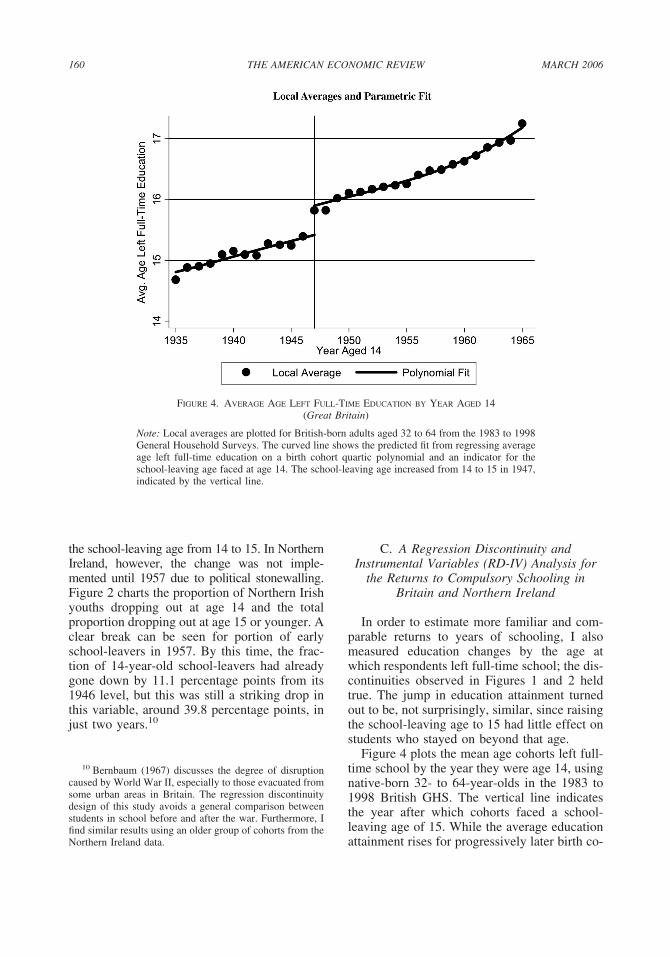
Figure 4 plots the mean age cohorts left full-time school by the year they were age 14, usingnative-born 32- to 64-year-olds in the 1983 to1998 British GHS. The vertical line indicatesthe year after which cohorts faced a school-leaving age of 15. While the average educationattainment rises for progressively later birth co-

10 Bernbaum (1967) discusses the degree of disruptioncaused by World War II, especially to those evacuated fromsome urban areas in Britain. The regression discontinuitydesign of this study avoids a general comparison betweenstudents in school before and after the war. Furthermore, Ifind similar results using an older group of cohorts from theNorthern Ireland data.

FIGURE 4. AVERAGE AGE LEFT FULL-TIME EDUCATION BY YEAR AGED 14(Great Britain)

Note: Local averages are plotted for British-born adults aged 32 to 64 from the 1983 to 1998General Household Surveys. The curved line shows the predicted fit from regressing averageage left full-time education on a birth cohort quartic polynomial and an indicator for theschool-leaving age faced at age 14. The school-leaving age increased from 14 to 15 in 1947,indicated by the vertical line.


horts, there is a clear spike in mean attainmentafter 1947. Average schooling increases by ex-actly half a year between the cohorts that wereage 14 in 1946 and in 1948. The figure alsoplots the fitted values from regressing the meanson a quartic polynomial for year of birth and anindicator term for whether or not a cohort faceda minimum school-leaving age of 15 (all 14-year-olds in 1947 and after). The fit predicts anincrease in education attainment between 1946and 1947 of 0.44 years (R2 � 0.995).11

This result, and the accompanying standarderror (0.065), can also be seen in column 1 ofTable 1, which was produced from the sameGHS data as the figures. The data were firstaggregated into cell means by birth cohort, re-gion, and age. All regressions are weighted bycell size and clustered by cohort and region(Britain or Northern Ireland) using Huber-White standard errors.12 Column 1 shows the

predicted break in education attainment of 0.44,corresponding to Figure 2A. The t-statistic forrejecting the discontinuity is 6.5.

Figure 5 shows the analogous graph forNorthern Ireland, where the school-leaving ageincreased from 14 to 15 in 1957. The plottedaverages are somewhat less smooth than forBritain because of the smaller sample size(R2 � 0.989). The quartic polynomial fit, alsopresented in Table 1, predicts an increase inaverage education attainment of 0.397 years in1957, indicated by the vertical line.

Figures 6 and 7 plot the corresponding rawmean log earnings for the British and NorthernIrish samples for 32- to 64-year-olds who were14 years old between 1935 and 1965. Earningsare measured in 1998 U.K. pounds using theRetail Price Index.13 Earnings from the com-

11 I also tried fitting the grouped means in several otherways: with a quadratic, with a quadratic allowed to differbefore and after 1947, and by omitting 14-year-olds in 1947,since not all faced a higher school-leaving age that year.These alternative specifications generate similar results.

12 Card and David S. Lee (2004) underscore the impor-tance of avoiding using conventional standard errors in adiscrete RD design, such as this one, which depends on aspecific functional form to compute the cohort trend.

13 Note that the cross-section panel of the 1983 to 1998panel includes fewer older cohorts at younger ages. Forexample, the GHS observes all those older than 51 whowere 14-year-olds in 1945, but only those 14-year-olds of1945 who are older than 61. This discrepancy does notaffect testing for a trend break in mean earnings followingthe introduction of the more restrictive school-leaving age,but it does lead to an upward trend in earnings for youngercohorts. To account for the sensitivity of the results to thedifferent age composition by birth cohorts, I also estimatethe discontinuity with age polynomial controls and age fixedeffects. Age fixed effects are possible with cohort effects

TABLE 1—ESTIMATED EFFECT OF MINIMUM SCHOOL-LEAVING AGE ON AGE FINISHED FULL-TIME EDUCATION AND LOG

ANNUAL EARNINGS

(Great Britain and Northern Ireland, ages 25–64, 1935–1965)

Sample population

(1) (2) (3) (4) (5) (6) (7)(First stage) dependent variable: Age

finished full-time school(Reduced form) dependent variable:

log annual earningsInitial

sample size

Great Britain 0.440 0.436 0.453 0.065 0.064 0.042 57264[0.065]*** [0.071]*** [0.076]*** [0.025]** [0.026]** [0.043]

Northern Ireland 0.397 0.391 0.353 0.054 0.074 0.074 8921[0.074]*** [0.073]*** [0.100]*** [0.27]* [0.025]*** [0.045]

G. Britain and N. Ireland withN. Ireland Fixed Effect

0.418 0.397 0.401 0.073 0.058 0.059 66185[0.040]*** [0.043]*** [0.045]*** [0.016]*** [0.016]*** [0.018]***

Birth Cohort PolynomialControls Quartic Quartic Quartic Quartic Quartic Quartic

Age Polynomial Controls None Quartic None None Quartic NoneAge Dummies No No Yes No No Yes

Notes: The dependent variables are age left full-time education and log annual earnings. Each coefficient is from a separateregression. Each regression includes controls for a birth cohort quartic polynomial and indicator whether a cohort faced aschool leaving age of 15 at age 14. Columns 2, 3, 5, and 6 also include age controls: a quartic polynomial and fixed effectswhere indicated. Each regression includes the sample of 25- to 64-year-olds from the 1983 through 1998 General HouseholdSurveys, who were aged 14 between 1935 and 1965. Data are first aggregated into cell means and weighted by cell size.Regressions are clustered by birth cohort and region (Britain or N. Ireland).


bined British GHS were 10.9 percent higher forcohorts aged 14 in 1948 than for those aged 14in 1946. The ratio of reduced form coefficientsfor these two groups is 0.279 (0.109/0.390). Thepolynomial fit in Figure 6, which includes aquartic cohort trend, predicts that average earn-ings increased by about 6.5 percent for thecohorts that come after the rise in the school-leaving age. Column 4 in Table 1 shows thisbreak is statistically significant, but the 95-percent confidence region around this value isconsiderably wide 0.016 to 0.114). The fittedincrease in log earnings for Northern Ireland in1957, however, is similar: a quartic fit with noage controls predicts an increase in log earningsof 0.054 points from raising the school-leavingage to 15. These point estimates are robust to

the inclusion of quartic age controls, shown incolumn 5 of Table 1. The confidence regionwidens somewhat with the inclusion of agefixed effects (shown in column 6), but generallythe results remain consistent with the trendsshown in the previous figures.

Table 2 calculates RD-IV estimates for bothBritain and Northern Ireland by regressingmean log earnings on a fourth-order polynomialcontrol for birth cohort, the average age a cohortleft full-time school, with this education mea-sure instrumented by the minimum school-leaving age a cohort faced at age 14. Allregressions use weighted cell means clusteredby cohort. These results are shown in column 4:the estimated average increase in earnings inBritain from raising the school-leaving age to 15is 14.7 percent. This figure corresponds to theWald estimate from dividing the estimated av-erage earnings discontinuity from Figure 6 bythe estimated education attainment discontinu-ity from Figure 4 (0.065/0.442). The compara-

because the GHS contains multiple years of cross-sectiondata. The results are also robust to the inclusion of surveyyear controls.

FIGURE 5. AVERAGE AGE LEFT FULL-TIME EDUCATION BY YEAR AGED 14(Northern Ireland)

Note: Local averages are plotted for Northern Irish adults aged 32 to 64 from the 1985 to 1998General Household Surveys. The curved line shows the predicted fit from regressing averageage left full-time education on a birth cohort quartic polynomial and an indicator for theschool-leaving age faced at age 14. The school-leaving age increased from 14 to 15 in 1957,indicated by the vertical line.


ble estimate for Northern Ireland is 13.5percent, and about 20 percent with the inclusionof age controls (see columns 5 and 6). Theseestimated effects are similar to previous returnsto compulsory schooling estimates, in particu-lar those presented in Harmon and Walker’s(1996) U.K. analysis.

The regression discontinuity approach leadsto some imprecision, given that earnings aretapering off for successively older birth cohortsat the time the discontinuity occurs. The analy-sis is strengthened, however, by moving to adifference-in-differences and instrumental-variables analysis by combining the two sets ofU.K. data. Doing so lowers the average fractionaffected by compulsory schooling a little, com-pared to using Britain alone, but the differenceis not great. The third row in Table 1 shows theestimated effects of raising the school-leavingage on the average age respondents left full-time school for the combined British and North-

ern Irish samples. Again I regressed averageeducation attainment on a quartic birth cohortcontrol, an indicator for the minimum school-leaving age a cohort faced, and now an indicatorfor Northern Ireland. The estimated increasein years of schooling from the higher school-leaving age with the combined data is 0.42years, compared to 0.44 using only the Britishsample. The standard error, however, falls con-siderably, to 0.04 (t-statistic � 13.6), and theresults are robust to including age controls(shown in columns 2 and 3).

Figure 8, which shows the correspondingcombined plots of British and Northern Irisheducation attainment by cohort, clearly illus-trates the differences in attainment before andafter the change in the school laws. Both re-gions follow almost identical upward trends inschooling until 1947, when Britain’s attainmentspikes. The average difference over the next tenyears remains constant at about 0.5 years, and

FIGURE 6. AVERAGE ANNUAL LOG EARNINGS BY YEAR AGED 14(Great Britain)

Note: Local averages are plotted for British-born adults aged 32 to 64 from the 1983 to 1998General Household Surveys. The curved line shows the predicted fit from regressing averagelog annual earnings on a birth cohort quartic polynomial and an indicator for the school-leaving age faced at age 14. The school leaving age increased from 14 to 15 in 1947, indicatedby the vertical line. Earnings are measured in 1998 U.K. pounds using the U.K. retail priceindex.


TABLE 2—OLS AND IV RETURNS TO (COMPULSORY) SCHOOLING ESTIMATES FOR LOG ANNUAL EARNINGS

(Great Britain and Northern Ireland, ages 25–64, 1935–1965)

(1) (2) (3) (4) (5) (6) (7)

Returns to schooling: OLS Returns to compulsory schooling: IVInitial

sample size

Great Britain 0.078 0.079 0.079 0.147 0.145 0.149 57264[0.002]*** [0.002]*** [0.002]*** [0.061]** [0.063]** [0.064]**

Northern Ireland 0.111 0.113 0.113 0.135 0.187 0.21 8921[0.004]*** [0.004]*** [0.004]*** [0.071]* [0.070]** [0.135]

G. Britain and N. Ireland withN. Ireland fixed effect

0.082 0.082 0.083 0.174 0.149 0.148 66185[0.001]*** [0.001]*** [0.001]*** [0.042]*** [0.044]*** [0.046]***

Birth cohort polynomialcontrols Quartic Quartic Quartic Quartic Quartic Quartic

Age polynomial controls None Quartic None None Quartic NoneAge dummies No No Yes No No Yes

Notes: The dependent variable is log annual earnings. Each regressions includes controls for a birth cohort quartic polynomialand age left full-time education (instrumented by an indicator whether a cohort faced a school leaving age of 15 at age 14in columns 4 through 6). Columns 2, 3, 5, and 6 also include age controls: a quartic polynomial and fixed effects whereindicated. Each regression includes the sample of 25- to 64-year-olds from the 1983 through 1998 General Household Surveyswho were aged 14 between 1935 and 1965. Data are first aggregated into cell means and weighted by cell size. Regressionsare clustered by birth cohort and region (Britain or N. Ireland).

FIGURE 7. AVERAGE ANNUAL LOG EARNINGS BY YEAR AGED 14(Northern Ireland)

Note: Local averages are plotted for Northern Irish adults aged 32 to 64 from the 1985 to 1998General Household Surveys. The curved line shows the predicted fit from regressing averagelog annual earnings on a birth cohort quartic polynomial and an indicator for the school-leaving age faced at age 14. The school-leaving age increased from 14 to 15 in 1957, indicatedby the vertical line. U.K. pounds using the U.K. retail price index.


the gap quickly narrows again after 1957, theyear when Northern Ireland increased itsschool-leaving age.

Combining the two sets of U.K. data alsohelps increase the precision in estimating thereduced-form effect on earnings. Figure 9 pre-sents the mean log earnings plots from Figures6 and 7 on the same grid. While the trend breaksfor Britain in 1947 and for Northern Ireland in1957 are apparent, comparing the two samplesreinforces these changes. The combined U.K.reduced form estimates for the average increasein earnings using quartic cohort and age con-trols are displayed in the third row of Ta-ble 1, columns 4 and 5. Again, estimates basedon the combined data are very similar to theseparate RD results: that raising the school-leaving age to 15 increased earnings, on aver-age, by about 5.5 or 7 percent, depending on theage controls used. This combined analysis al-lows for more robust results than the individualcalculations, with a considerably lower standarderror.

Table 2 shows IV estimates corresponding tothe data displayed in Figures 8 and 9. Column 4of the third row shows that, without age con-trols, raising the school-leaving age is associ-ated with a 17.4-percent increase in earnings.Adding a quartic age control (column 5) or agefixed effects (column 6) lowers this estimate to14.9 percent.

The OLS results shown in columns 1 to 3 arelower, consistent with many previous IV andOLS comparisons. It may seem surprising thatthe OLS results differ from the IV results forBritain, since the law change had an impact onmuch of the same group used to estimate theOLS results. But these results assume linearreturns to all levels of schooling. If we restrictthe OLS sample to only those who left school atage 16 or before, the resulting OLS estimatesare more similar to the IV. The OLS estimatescorresponding to columns 1, 2, and 3 for thisrestricted sample of early school leavers are14.5, 14.1, and 14.0, respectively. Thus, whileOLS and IV results for the high school dropout

FIGURE 8. AVERAGE AGE LEFT FULL-TIME EDUCATION BY YEAR AGED 14(Great Britain and Northern Ireland)

Note: The upper dark line shows the average age left full-time education by year aged 14 forBritish-born adults aged 32 to 64 from the 1983 to 1998 General Household Surveys. Thelower light line shows the same, but for adults in Northern Ireland.


sample are similar—which is not surprisinggiven the large fraction in this sample affectedby the school-leaving age—the OLS returns forthose older than the school-leaving age are stillsmaller than the IV results.

III. A Cross-Country Comparison

In this section, I move across the Atlantic toconsider the returns to compulsory schooling inNorth America and how they compare with theresults for the United Kingdom. After a briefdiscussion of my Canadian and U.S. datasources, I show that the effects on educationattainment from changes in the minimumschool-leaving age in the United States andCanada were much smaller than for the UnitedKingdom. I then look at how the LATE com-pares across countries. The fact that my findingsare reasonably similar suggests the LATE andATE for high school may also be reasonablysimilar.

A. North American Data

Specific details of the U.S. and Canadian dataextracts are provided in the Data Appendix.Wherever possible, I tried to maintain consis-tency in sample selection, school laws, and vari-able definitions across countries. The samplesinclude all 25- to 64-year-old males and femaleswho were age 14 in the years that the school-leaving ages were available (1915 to 1970 forthe United States, and 1925 to 1970 for Can-ada). The U.S. analysis uses all native-bornindividuals age 25 to 64 from the six decennialcensus microdata samples from 1950 through2000, and the Canadian data use native-born 25-to 64-year-olds from the 33-percent sample ofthe 1971 Census, and the five 20-percent sam-ples of the 1981 through 2001 Censuses. Forboth countries, individuals are matched to theminimum school-leaving age in their state orprovince of birth the year that they were age 14.I also matched to each individual a number of

FIGURE 9. AVERAGE LOG ANNUAL EARNINGS BY YEAR AGED 14(Great Britain and Northern Ireland)

Note: The upper dark line shows the average log annual earnings by year aged 14 forBritish-born adults aged 32 to 64 from the 1983 to 1998 General Household Surveys. Thelower light line shows the same, but for adults in Northern Ireland.


regional controls. For the United States, theseincluded average age, as well as the fractions ofthe population in each state that lived in anurban city, lived on a farm, was black, was inthe labor force, and worked in the manufactur-ing industry. For Canada, I matched average percapita school and public expenditures and frac-tions of the population in each province thatlived in urban areas and worked in the manu-facturing sector.14 I collapsed both datasets intocell means by state or province, birth cohort,census year, and gender.

B. The Effect of School-Leaving Laws onSchool Attainment

Table 3 presents the first-stage effects of theschool-leaving age changes on education attain-ment and the corresponding reduced form ef-fects of the school-leaving age on earnings. Thefirst panel shows results for the United States,and the second for Canada; the third showscomparable results from the combined British–Northern Irish sample. All data are aggregatedinto cell means and weighted by population size.All regressions include fixed effects for birth year,region, survey year, gender, race, and a quartic inage—and additional regional demographic andeconomic controls according to when cohortswere age 14. The fourth panel repeats the regres-sion discontinuity results for Britain, discussed inSection IIC. Since cohort fixed effects are notidentified while trying to estimate the compulsoryschooling effect, I use instead a quartic to controlfor cohort trends and age fixed effects, as before.

Column 1 shows the estimated impact fromraising the school-leaving age on the total num-ber of years of completed schooling. Note thatthe impact is much smaller for the United Statesand Canada than for the United Kingdom: rais-ing the minimum school-leaving age by oneyear increased education attainment by onlyabout 0.11 years. Furthermore, both Lochnerand Moretti (2004) and I (Oreopoulos, 2003)find additional effects from compulsory school-ing on education attainment beyond the mini-mum requirements for North America. Students

compelled to stay in school an extra year whoend up staying beyond the new limit push theestimated effect in column 1 higher, so thefraction actually affected by compulsoryschooling in these countries may be smaller.(This situation differs from that in the UnitedKingdom; as discussed in the last section,Figures 1 and 2 show that raising the school-leaving age from 14 to 15 had no noticeableimpact on students finishing beyond age 15.)The first-stage effect for all countries is consid-erably powerful, and we easily reject that thecoefficients are zero.

Comparing columns 2 and 3 of Table 3 pro-vides a specification check for whether otherregion-specific policies or economic conditionsimproved at the same time that minimumschool-leaving ages increased. It is reassuringthat law changes have no positive effect on thefraction of individuals who attained at leastsome post-secondary education or who leftschool beyond age 17 (column 3).15 The coef-ficients for the samples of those with fewer than12 years of completed schooling and of thosewho finished school by age 16 are about thesame (column 2), as we would expect if thosecompelled to take additional schooling by changesin these laws still dropped out, only later.16

The last three columns show the reduced-form estimates for the effects of these dropoutages on earnings and wages. The main purposeof showing these results is to demonstrate thatchanges in the dropout age do not affect earn-ings in the post-secondary sample. Just as weshould not expect compulsory schooling laws toaffect post-secondary-schooling attainment, weshould not expect them to affect outcome vari-ables for the higher educated sample. If we didobserve either of these effects, we might beconcerned that other factors, ones affecting bothdropouts and graduates, underlie the correla-tions in Table 1. While the laws are strongly

14 Results were not very sensitive to the inclusion ofalternative controls. Below I display the LATE estimateswith and without the control variables, and with and withoutcohort trends.

15 The fourth panel of Table 3 shows that in the Britishsample very few students stayed in school beyond age 16,which makes it hard to draw any conclusions about thecorresponding coefficient in column 3.

16 The results also suggest that changes in U.S. school-leaving laws influenced would-be dropouts to graduate. Ifwe restrict the initial sample to those with 12 or fewer yearsof completed schooling, the findings are very similar tothose from using the full sample.


related to earnings among dropouts, column 6shows no noticeable relationship between theminimum schooling a cohort faced when youngand its average earnings for the post-secondary-school sample. These results are also suggestivethat raising high school attainment had no re-gion-specific externalities on the birth cohortsthat attained post-secondary school.17

C. The LATE of Compulsory Schooling forthe United States, Canada, and the United

Kingdom

I estimate that dropouts compelled to take anadditional year of high school earn about 10 to14 percent more than dropouts without theadditional year. The returns to compulsory-schooling estimates are similar across allcountries, whether restricting the initial sampleby gender or by race. The effects generallyappear to be the largest for the United Kingdom

17 For more specification checks to the robustness ofthese results, see Oreopoulos (2003).

TABLE 3—FIRST-STAGE EFFECTS OF COMPULSORY SCHOOLING ON EDUCATION ATTAINMENT AND EARNINGS FOR THE UNITED

STATES, CANADA, AND THE UNITED KINGDOM

(1) (2) (3) (4) (5) (6)First-stage effects of dropout ages on schooling Reduced form coefficients on earnings

Full sampleSample with

� high schoolSample with

� high school Full sampleSample with

� high schoolSample with

� high school

United States [1901–1961 birth cohorts aged 25–64 in the 1950–2000 Censuses]Dependent variable

Number of years of schooling Log weekly wageMinimum school-leaving age

at age 140.110 0.100 0.003 0.016 0.010 0.003

[0.0070]*** [0.0097]*** [0.0027] [0.0015]*** [0.0024]*** [0.0017]*Initial sample size 2,814,203 727,789 1,173,880F-test: Schl.-leaving age coeff.

is zero 243.5Canada [1911–1961 birth cohorts aged 25–64 in the 1971–2001 Censuses]

Dependent variableNumber of years of schooling Log annual wage

Minimum school-leaving ageat age 14

0.130 0.130 �0.026 0.012 0.012 �0.003[0.0154]*** [0.0129]*** [0.0114]** [0.0037]*** [0.0047]** [0.0049]

Initial sample size 854,243 355,299 298,342F-test: Schl.-leaving age coeff.

is zero 70.5United Kingdom [1921–1951 birth cohorts aged 32–64 in the 1983–1998 GHHS]

Dependent variableAge left full-time education Log annual wage


0.369 0.487 0.062 0.058 0.052 0.005[0.0305]*** [0.0309]*** [0.0785] [0.0198]*** [0.0242]** [0.0369]


is zero 184.9Britain [1921–1951 birth cohorts aged 32–64 in the 1983–1998 GHHS]

Dependent variableAge left full-time education Log annual wage


0.453 0.483 0.351 0.042 0.045 �0.014[0.076]*** [0.0868]*** [0.2412] [0.043] [0.0387] [0.0542]


is zero 36.0

Note: Regressions in the top three panels include fixed effects for birth year, region (state, province, Britain/N. Ireland),survey year, sex, and a quartic in age. The U.S. results also include a dummy variable for race, and state controls for fractionsliving in urban areas, black, in the labor force, in the manufacturing sector, female, and average age based on when a birthcohort was age 14. Provincial controls for Canada include fractions in urban areas, in the manufacturing sector, and controlsfor per capital public and school expenditures. Data are grouped into means by birth year, nation, sex, race (for the U.S.) andsurvey year and weighted by cell population size. Huber-White standard errors are shown from clustering by region and birthcohort. Single, double, and triple asterisks indicate significant coefficients at the 10-percent, 5-percent, and 1-percent levels,respectively. The omitted variable indicates ability to drop out at age 13 or lower for the U.S. and Canada, and 14 or less forthe U.K. Samples include all adults aged 25 to 64. Dependent variable in column 3 for Canada is 1 � some post-secondaryschooling, 0 otherwise. The last panel shows results with only the British sample, using a quartic birth cohort polynomialinstead of cohort fixed effects. See text for more data specifics.


sample, though the associated standard errorsare high. Overall, there is no evidence that theU.S. or Canadian effects are higher than theBritish ones, except perhaps for U.S. blackmales.

The detailed IV estimates for the returns tocompulsory schooling are shown in Table 4.Column 2 includes the IV results correspondingto the first and second stages in columns 1 and2 of Table 3. All regressions in the first threepanels include a quartic in age and fixed effectsfor birth cohort, region, survey year, and gen-der. The U.S. results also include a dummyvariable for race; a number of state controls(fraction of state that lives in urban areas, is

black, is in the labor force, works in the manu-facturing sector, is female); and a variable foraverage age based on when the birth cohort wasage 14. Province controls were used for Canada,including the fraction of the province that livesin urban areas and works in the manufacturingsector, as well per capita public and schoolexpenditures. Data are grouped into means bybirth year, region, gender, race (for the UnitedStates), and survey year. Huber-White standarderrors are shown from clustering by region andbirth cohort. The IV-RD results for Britain arerepeated in the fourth panel of Table 4 andinclude a quartic cohort control and age fixedeffects.

TABLE 4—OLS, IV-DD, AND IV-RD ESTIMATES OF THE RETURNS TO (COMPULSORY) SCHOOLING FOR THE UNITED STATES,CANADA, AND THE UNITED KINGDOM

(1)OLS

full sample

(2)IV with

regional controls

(3)IV with

regional trends

(4)IV with

regional trends andregional controls

Dependent variable United States [1901–1961 birth cohorts aged 25–64 in the 1950–2000 censuses]Log weekly earnings (all workers) 0.078 0.142 0.175 0.405

[0.0005]*** [0.0119]*** [0.0426]*** [0.7380]Log weekly earnings (males) 0.070 0.127 0.074 0.235

[0.0004]*** [0.0145]*** [0.0384]* [0.1730]Log weekly earnings (black males) 0.074 0.172 0.119 0.264

[0.0004]*** [0.0137]*** [0.0306]*** [0.1295]**Canada [1911–1961 birth cohorts aged 25–64 in the 1971–2001 censuses]

Log annual earnings (all workers) 0.099 0.096 0.095 0.142[0.0007]*** [0.0254]*** [0.1201] [0.0652]**

Log annual earnings (males) 0.087 0.124 �0.383 0.115[0.0008]*** [0.0284]*** [1.1679] [0.0602]*

United Kingdom [1921–1951 birth cohorts aged 32–64 in the1983–1998 GHHS]

Log annual earnings (all workers) 0.079 0.158 0.195 NA[0.0024]*** [0.0491]*** [0.0446]***

Log annual earnings (males) 0.055 0.094 0.066 NA[0.0017]*** [0.0568] [0.0561]

Britain [1921–1951 birth cohorts aged 32–64 in the 1983–1998 GHHS]OLS RD

Log annual earnings (all workers) 0.078 0.147 NA NA[0.002]*** [0.061]**

Log annual earnings (males) 0.055 0.150 NA NA[0.0017]*** [0.130]

Note: Regressions in the top three panels include fixed effects for birth year, region (state, province, Britain/N. Ireland),survey year, sex, and a quartic in age. The U.S. results also include a dummy variable for race, and state controls for fractionsliving in urban areas, black, in the labor force, in the manufacturing sector, female, and average age based on when a birthcohort was age 14. Provincial controls for Canada include fraction in urban areas, in the manufacturing sector, and controlsfor per capita public and school expenditures. Data are grouped into means by birth year, nation, sex, race (for the U.S.) andsurvey year and weighted by cell population size. Huber-White standard errors are shown from clustering by region and birthcohort. Single, double, and triple asterisks indicate significant coefficients at the 10-percent, 5-percent, and 1-percent levels,respectively. The omitted variable indicates ability to drop out at age 13 or lower for the U.S. and Canada, and 14 or less forthe U.K. Samples include all adults aged 25 to 64. The last panel repeats regression discontinuity results from Table 2 usingthe British sample only and a quartic birth cohort polynomial instead of cohort fixed effects. See text for more data specifics.


The results are robust to including linear re-gion-specific cohort trends (see columns 3 and 4of Table 4). These were included to control forrelative changes in education attainment orearnings over time that differ by state or prov-ince, or between Northern Ireland and Britain,and are not due to changes from compulsoryschool laws. The regressions, however, uninten-tionally absorb some of the effects of compul-sory schooling if schooling or earnings trendover time in a nonlinear way, or if the effectsfrom the minimum school-leaving age take timeto become fully enforced. Table 4, column 3,shows coefficient estimates after including lin-ear region-cohort trends, but drops the regionalcontrol variables already included in column 2.Including these trends produces point estimatesthat are less precise—some smaller and somelarger than in column 2—but not very differentfrom before. Column 4 includes both regionalcohort trends and the previous regional controls.Including both controls leads to multicollinear-ity, since regional changes in demographics andeconomic conditions both try to capture overalldifferences in regions over time. The range ofpossible true values for returns to schoolingshown here is so wide that we cannot draw anymeaningful conclusions from the results in thiscolumn.

The comparable full sample OLS results areshown in Table 4, column 1. I aggregated thecountry data also by level of schooling to cal-culate these results (still weighted by cell sam-ple size). For all countries, OLS point estimatesare significantly lower than the IV results.Across countries, however, the IV results arenot very different, even though the proportionaffected by changes in the school-leaving age inthe United Kingdom exceeded that in the UnitedStates and Canada by 35 percentage points ormore.

The results presented in Table 5 show othereffects from compulsory schooling. Health out-comes are strongly associated with minimumschool-leaving age changes, corroborating Lleras-Muney’s (2002) finding that schooling lowersmortality. The 1990 and 2000 U.S. Censusesask questions about physical and mental healthlimitations. Over 9 percent of the individuals inthe sample aged 25 to 84 claim a physical ormental health disability that limits their per-sonal care; I estimate that an additional year of

compulsory schooling lowers the likelihood ofreporting such a disability by 1.7 percentagepoints, a figure that is similar to the OLS esti-mate. Another year of compulsory schoolingalso lowers the likelihood of reporting a disabil-ity that limits one’s daily activity by 2.5 per-centage points. In the United Kingdom, theGHS questionnaire asks respondents to self-report whether they are in good, fair, or poorhealth. A one-year increase in schooling lowersthe probability that a respondent reports beingin poor health by 3.2 percentage points, andraises the chances he or she reports being ingood health by 6 percentage points.

Schooling also affects many labor marketoutcomes in addition to earnings. In all threecountries, I find that compulsory schooling low-ers the likelihood of respondents being in thelabor force and looking for work. The magni-tude of the effect is similar across countries, andalso comparable to corresponding OLS esti-mates. Further compulsory schooling also low-ers the likelihood of receiving welfare and beingclassified as poor. Dropouts who drop out oneyear later are 6 percentage points less likely tofall below the U.S. poverty line and 3 percent-age points less likely to fall below Canada’slow-income cutoff.18

IV. Discussion and Conclusion

Because most students in the United King-dom at mid-century tended to leave school atthe earliest legal age, studying the effects ofraising this age from 14 to 15 allowed me toestimate local average treatment effects of edu-cation that come close to mirroring averagetreatment effects. The regression discontinuitydesign of my U.K. analysis avoids having toassume unobservable trends in regional charac-teristics that could also affect the outcomes.Comparing LATE estimates for North America,where few students were affected by compul-sory school laws, to the U.K. estimates providesa test of whether IV returns to schooling oftenexceed OLS because gains are high only forsmall and peculiar groups among the more gen-

18 A household falls below the low-income cutoff if itspends more than 20 percentage points above the averagecomparative household on food, clothing, and shelter.


eral population. I find, instead, that the gainsfrom compulsory schooling are very large—between 10 and 14 percent—whether these lawsaffect a majority or minority of those exposed.

This finding of high returns to compulsoryschooling raises the question of why dropoutsdrop out in the first place. Why did so manyleave school in the United Kingdom if stayingon would have led to substantial gains, on av-erage, to labor market and health outcomes?

One possibility, sometimes used to explainwhy IV returns to schooling estimates exceed

OLS, is that individuals dropping out are credit-constrained. Considering the similarity of IVresults across countries, this explanation couldapply only if students from the United Kingdomtend to face greater financial constraints fromstaying on than students from the United Statesand Canada. As I discuss in Section II, however,while about half of secondary students in Brit-ain paid some fees to attend school, the removalof these fees in 1944 did not affect attainmentbeyond age 15. Furthermore, many early schoolleavers do not work. Among 15- and 16-year-

TABLE 5—OLS AND IV ESTIMATES FOR EFFECTS OF (COMPULSORY) SCHOOLING ON SOCIALECONOMIC OUTCOMES

(1)Mean

� HS sample(2)

OLS

(3)IV

full sample

Country (schooling variable)Health outcomes (ages 25–84)

United States (total years of schooling)Physical or mental health disability that limits personal care 0.092 �0.014 �0.025

[0.0003]*** [0.0058]***Disability that limits mobility 0.128 �0.020 �0.043

[0.0004]*** [0.0070]***United Kingdom (age left full-time education)

Self reported poor health 0.150 �0.037 �0.032[0.0016]*** [0.0113]***

Self reported good health 0.564 0.065 0.060[0.0021]*** [0.0155]***

Other socialeconomic outcomes (ages 25–64)United States (schooling variable: total years of schooling)

Unemployed 0.064 �0.004 �0.005[0.0002]*** [0.0040]

Receiving welfare 0.067 �0.013 �0.011[0.0002]*** [0.0024]***

Below poverty line 0.220 �0.023 �0.064[0.0002]*** [0.0085]***

Canada (total years of schooling)Unemployed: looking for work 0.062 �0.038 �0.010

[0.0044]*** [0.003]***Below low-income cutoff 0.227 �0.038 �0.026

[0.0004]*** [0.0038]***United Kingdom (age left full-time education)

In labor force: looking for work 0.110 �0.030 �0.032[0.0044]*** [0.0150]**

Receiving income support 0.066 �0.025 �0.059[0.0024]*** [0.0259]**

Note: All regressions include fixed effects for birth year, region (state, province, Britain/N. Ireland), survey year, sex, and aquartic in age. The U.S. results also include a dummy variable for race, and state controls for fractions living in urban areas,black, in the labor force, in the manufacturing sector, female, and average age based on when a birth cohort was age 14.Provincial controls for Canada include fraction in urban areas, in the manufacturing sector, and controls for per capital publicand school expenditures. Data are grouped into means by birth year, nation, sex, race (for the U.S.) and survey year andweighted by cell population size. Huber-White standard errors are shown from clustering by region and birth cohort. Single,double, and triple asterisks indicate significant coefficients at the 10-percent, 5-percent, and 1-percent levels, respectively. Seetext for more data specifics.


olds recorded in the 1950 U.S. Census as not inschool, fewer than half (41 percent) were in thelabor force and 89 percent lived with theirparents.19

Several alternative explanations for dropoutbehavior exist. First, dropouts may simply ab-hor school. Poor classroom performance andcondescending attitudes from students andteachers may make students want to leave assoon as possible, even at the expense of forgo-ing large monetary sums (Valerie E. Lee andDavid T. Burkam, 2003). Second, the uncer-tainty of additional earnings from staying onmay be too high. If a student is risk-averse,higher expected returns from additional school-ing may not be enough to offset higher proba-bilities of earning particularly low wages(David Levhari and Yoram Weiss, 1974; StaceyH. Chen, 2001). A third alternative is that drop-outs may ignore or severely discount futureconsequences of their decisions (e.g., TedO’Donoghue and Matthew Rabin, 1999). Cul-tural or peer pressures might also predominateadolescent decision-making and lead to dropoutbehavior; cultural norms that devalue schooling,a lack of emotional support, and low acceptancefor higher education among peers may exacer-bate students’ distaste for school beyond theminimum age (e.g., George A. Akerlof andRachel E. Kranton, 2002; and James C.Coleman, 1961). A final consideration is thatstudents may simply mispredict, making incor-rect present-value calculations of future returnsor else underestimating the real gains of in-creased schooling.

We cannot determine with this paper’s anal-ysis which of these reasons might matter most,since the effects of compulsory schoolingexamined here arise only after leaving school,and costs (pecuniary and nonpecuniary) arenot examined. But each explanation carriesquite different implications about educationpolicy. Exploring these issues more directlythrough innovative field experiments or bygathering data on high school students’ ex-pectations on gains and costs from staying onlonger may shed further light on understand-

ing dropout behaviour and, more generally,the overall education attainment decision-making process.

DATA APPENDIX

A. The United States

Most of the U.S. analysis uses an extract ofnative-born individuals aged 25 to 64 from thesix decennial census microdata samples be-tween 1950 and 2000.20 All censuses containedindividual wages, poverty status, and laborforce participation, but only the 1990 and 2000datasets contained disability outcome measures.The initial sample size among those with posi-tive wages was 2,814,203. After collapsingthese into cell means, there were 29,804 cells bystate, birth cohort, census year, and gender, and15,003 cells among males. Hawaiian- and Alas-kan-born respondents were excluded.

I coded the schooling variable for individualsin the 1950–1980 data as highest grade com-pleted, capped at 17 to impose a uniform top-code across censuses. Following Acemoglu andAngrist (2001), average years of schooling wereassigned to categorical values in the 1990 and2000 Censuses using the imputation for malesand females in Jin Huem Park (1999). Theearnings variable, log weekly wage, was calcu-lated by dividing annual wage and salary in-come by weeks worked, then taking logs.

The cell groups were assigned a minimumschool-leaving age according to the year inwhich members of a birth cohort were 14 yearsold and the state in which they were born.21 Imeasured each school-leaving age as the mini-

19 Fifty years later, the pattern has not changed much.Among 17-year-olds not in school, according to the 2000U.S. Census, for example, 90.4 percent lived with parents,and 45 percent were not in the labor force.

20 The specific datasets used were the 1950 General1/330 sample (limited to those with long-form responses),the 1960 General 1-percent sample, the 1970 Form 2 State1-percent sample, the 1980 Metro 1-percent sample, the1990 1-percent unweighted sample, and the 2000 1-percentunweighted random sample.

21 My analysis assumes that Americans went to school intheir state of birth, Canadians went to school in their prov-ince of birth, British-born residents went to school in Brit-ain, and Northern Irish residents went to school in NorthernIreland. Some individuals will be mismatched. If mobilityacross regions is unrelated with law changes, this measure-ment error will not bias our estimates. Lleras-Muney (2005)concludes this seems to be the case for the United States.


mum between a state’s legislated dropout ageand the minimum age required to obtain a work-ing permit.22 During this period, a few stateshad no laws in place. I grouped the 2.2 percentof the sample that faced school-leaving ageslower than 14 into one category (school-leavingage � 14). All others faced dropout ages of 14,15, or 16. The laws changed frequently over thisperiod, both across states and within states overtime. About one-third of the variation in theschool-leaving age is across states and two-thirds is within. Not all changes were positive;in some instances the minimum school-leavingage went down.

I also generated control variables for stateeconomic and demographic conditions in theyear the laws were in place. For each censusbetween 1910 and 1980, I calculated the aver-age age of the population in each state, as wellas the fraction living in an urban city, living ona farm, black, in the labor force, and working inthe manufacturing industry. Values between de-cades were generated by linear interpolation.

B. Canada

The data extract for Canada comes from thefour public-use micro-data censuses from 1981to 1996. The main extract contained 25- to64-year-olds born in a Canadian province whowere 14 years old between 1925 and 1975.While provincially legislated school-leavingages were available for earlier years, I chose tobegin with 1925 for two reasons: the cohortsaged 14 before 1925 were older than 55 in the1971 Census, and compulsory school laws wereoften minimally enforced at the beginning of thecentury. The initial sample size among thosewith positive wages was 854,243. After collaps-ing the data into province, birth cohort, gender,and census groups, the cell sample size was3,296 among males and females, and 1,648among males.

The education variable used for the Canadiananalysis was total years of schooling, whichrefers to the total sum of the years (or grades) ofschooling at the elementary, secondary, univer-sity, and nonuniversity years. I used the log ofannual wages and salaries as the earnings vari-able for the Canadian data. I did not convert thisvariable to weekly earnings because a consid-erable number of full-time workers excludedtheir paid vacations or sick leave when report-ing number of weeks worked in the previousyear, contrary to census instructions.

The school-leaving laws were compiled di-rectly from provincial statutes and revised stat-utes containing the acts of legislation and theiramendments since inception. In a previousstudy, I documented the history of these changesand other compulsory school laws extensively(Oreopoulos, forthcoming). A few provinces inthe first half of the century legislated differentdropout ages for urban and for rural areas. Forthese cases, I recorded the dropout age as thatfor rural areas, since for most of that period themajority of residents lived in rural areas. Allprovinces except British Columbia experiencedlegislated increases in the school-leaving ageduring the period under study. Most provincesallowed for working permit exceptions to theage laws, but they were rarely applied. Fewerthan 12 percent of the sample faced a school-leaving age of 16. I chose to group individualsfacing a school-leaving age of either 15 or 16,since the effect on grade attainment from raisingthe school-leaving age to 16 from 15 was notsignificantly different from zero and was impre-cisely measured. Including an indicator for fac-ing a school-leaving age equal to 16 did notalter the second-stage estimates.

As with the U.S. extract, I generated controlvariables for provincial economic and demo-graphic conditions using historical tabulationsand linear interpolation. Oreopoulos (forthcom-ing) describes these control variables in moredetail.

REFERENCES

Acemoglu, Daron and Angrist, Joshua D. “HowLarge Are Human-Capital Externalities? Ev-idence from Compulsory Schooling Laws,”in Ben S. Bernanke and Kenneth, eds., Ro-goff, NBER macroeconomics annual 2000.

22 Acemoglu and Angrist (2001), Lleras-Muney (2005),and Claudia Goldin and Lawrence Katz (2003) find workingpermit restrictions were often more binding than school-leaving age restrictions. The results are not sensitive tousing just the dropout age as the compulsory school lawvariable, or the predicted mandatory number of schoolyears, used by Acemoglu and Angrist (2001) and Lochnerand Moretti (2004).


Cambridge, MA: MIT Press, 2001, pp. 9–59.Akerlof, George A. and Kranton, Rachel E.

“Identity and Schooling: Some Lessons forthe Economics of Education.” Journal of Eco-nomic Literature, 2002, 40(4), pp. 1167–1201.

Angrist, Joshua D. “Treatment Effect Heteroge-neity in Theory and Practice.” EconomicJournal, 2004, 114(494), pp. C52–83.

Angrist, Joshua D. and Krueger, Alan B. “DoesCompulsory School Attendance AffectSchooling and Earnings?” Quarterly Journalof Economics, 1991, 106(4), pp. 979–1014.

Angrist, Joshua D. and Krueger, Alan B. “Empir-ical Strategies in Labor Economics,” in OrleyAshenfelter and David Card, eds., Handbookof labor economics. Vol. 3A. Amsterdam:Elsevier Science, North-Holland, 1999, pp.1277–366.

Barnard, Howard C. A history of English edu-cation from 1760. 2nd ed. London: Univer-sity of London Press, 1961.

Bernbaum, Gerald. Social change and theschools, 1918–1944. London: Routledge andK. Paul, 1967.

Bound, John; Jaeger, David A. and Baker, ReginaM. “Problems with Instrumental VariablesEstimation when the Correlation between theInstruments and the Endogenous ExplanatoryVariable Is Weak.” Journal of the AmericanStatistical Association, 1995, 90(430), pp.443–50.

Cameron, Stephen V. and Taber, Christopher.“Estimation of Educational Borrowing Con-straints Using Returns to Schooling.” Journalof Political Economy, 2004, 112(1), pp. 132–82.

Card, David. “Using Geographic Variation inCollege Proximity to Estimate the Return toSchooling,” in Louis N. Christofides, E. Ken-neth Grant, and Robert Swidinsky, eds., As-pects of labour market behaviour: Essays inhonour of John Vanderkamp. Toronto: Uni-versity of Toronto Press, 1995, pp. 201–22.

Card, David. “Estimating the Return to School-ing: Progress on Some Persistent Economet-ric Problems.” Econometrica, 2001, 69(5),pp. 1127–60.

Card, David and Lee, David S. “Regression Dis-continuity Inference with Specification Er-ror.” University of California, Berkeley,Center for Labor Economics Working Paper:No. 74, 2004.

Carneiro, Pedro and Heckman, James J. “TheEvidence on Credit Constraints in Post-Secondary Schooling.” Economic Journal,2002, 112(482), pp. 705–34.

Chen, Stacey H. “Is Investing in College Educa-tion Risky?” State University of New York atAlbany, Department of Education DiscussionPapers: No. 01-09, 2001.

Chiswick, Barry R. “Minimum Schooling Leg-islation and the Cross-Sectional Distributionof Income.” Economic Journal, 1969,79(315), pp. 495–507.

Coleman, James S. The adolescent society. NewYork: The Free Press, 1961.

Cruz, Luiz M. and Moreira, Marcelo J. “On theValidity of Econometric Techniques withWeak Instruments: Inference on Returns toEducation Using Compulsory School Atten-dance Laws.” Journal of Human Resources,2005, 40(2), pp. 393–410.

Cusick, Philip. Inside high school: The student’sworld. New York: Holt, Rinehart, and Winston,1972.

Dent, Harold C. Growth in English education:1946–1952. London: Routledge and KeganPaul, 1954.

Dent, Harold C. The Education Act: 1944. Lon-don: University of London Press, 1957.

Dent, Harold C. 1870–1970: Century of growthin English education. London: LongmanGroup Limited, 1970.

Dent, Harold C. The educational system ofEngland and Wales. London: University ofLondon Press, 1971.

Dominitz, Jeff and Manski, Charles F. “UsingExpectations Data to Study Subjective In-come Expectations.” Journal of the AmericanStatistical Association, 1997, 92(439), pp.855–67.

Durcan, Thomas J. History of Irish educationfrom 1800. Bala, Wales, UK: Dragon Books,1972.

Godsen, P. H. J. H. How they were taught: Ananthology of contemporary accounts of learn-ing and teaching in England 1800–1950. Ox-ford: Basil Blackwell, 1969.

Goldin, Claudia and Katz, Lawrence. “Mass Sec-ondary Schooling and the State.” NationalBureau of Economic Research, Inc., NBERWorking Papers: No. 10075, 2003.

Halsey, Albert H.; Heath, Anthony F. and Ridge,John M. Origins and destinations: Family,


class, and education in modern Britain. Ox-ford: Clarendon Press, 1980.

Harmon, Colm and Walker, Ian. “Estimates ofthe Economic Return to Schooling for theUnited Kingdom.” American Economic Re-view, 1995, 85(5), pp. 1278–86.

Heckman, James J. “Instrumental Variables: AStudy of Implicit Behavioral AssumptionsUsed in Making Program Evaluations.” Jour-nal of Human Resources, 1997, 32(3), pp.441–62.

Heckman, James and Vytlacil, Edward. “CausalParameters, Structural Equations, TreatmentEffects and Randomized Evaluation of SocialPrograms.” Unpublished Paper, 2001.

Imbens, Guido W. and Angrist, Joshua D. “Iden-tification and Estimation of Local AverageTreatment Effects.” Econometrica, 1994,62(2), pp. 467–75.

Kane, Thomas J. and Rouse, Cecilia Elena. “La-bor-Market Returns to Two- and Four-YearCollege.” American Economic Review, 1995,85(3), pp. 600–14.

Lang, Kevin. “Ability Bias, Discount Rate Bias,and the Return to Education.” UnpublishedPaper, 1993.

Lee, Valerie E. and Burkam, David T. “DroppingOut of High School: The Role of SchoolOrganization and Structure.” American Edu-cational Research Journal, 2003, 40(2), pp.353–93.

Levhari, David and Weiss, Yoram. “The Effect ofRisk on the Investment in Human Capital.”American Economic Review, 1974, 64(6), pp.950–63.

Lleras-Muney, Adriana. “Were Compulsory At-tendance and Child Labor Laws Effective?

An Analysis from 1915 to 1939.” Journal ofLaw and Economics, 2002, 45(2), pp. 401–35.

Lleras-Muney, Adriana. “The Relationship be-tween Education and Adult Mortality in theUnited States.” Review of Economic Studies,2005, 72(1), pp. 189–221.

Lochner, Lance and Moretti, Enrico. “The Effectof Education on Crime: Evidence fromPrison Inmates, Arrests, and Self-Reports.”American Economic Review, 2004, 94(1), pp.155–89.

O’Donoghue, Ted and Rabin, Matthew. “Doing ItNow or Later.” American Economic Review,1999, 89(1), pp. 103–24.

O’Keeffe, Dennis J. “Some Economic Aspects ofRaising the School Leaving Age in Englandand Wales in 1947.” Economic History Re-view, Second Series, 1975, 28(3), pp. 500–16.

Oreopoulos, Philip. “Do Dropouts Drop Out TooSoon? International Evidence from Changesin School-Leaving Laws.” National Bureauof Economic Research, Inc., NBER WorkingPapers: No. 10155, 2003.

Oreopoulos, Philip. “The Compelling Effects ofCompulsory Schooling: Evidence from Can-ada.” Canadian Journal of Economics, 2006,39(1) (forthcoming).

Park, Jin Huem. “Estimation of Sheepskin Ef-fects Using the Old and New Measures ofEducational Attainment in the Current Popu-lation Survey.” Economics Letters, 1999,62(2), pp. 237–40.

Staiger, Douglas and Stock, James H. “Instru-mental Variables Regression with Weak In-struments.” Econometrica, 1997, 65(3), pp.557–86.


Documents

Estimating Average and Local Average Treatment …faculty.smu.edu/millimet/classes/eco7321/papers/...change. The break in education attainment is so stark in both Britain and Northern