Estimating Annual and Monthly Supply and Demand for World Oil:

A Dry Hole?

C.-Y. Cynthia Lin1 Preliminary—Comments Welcome

Abstract

This paper uses instrumental variables and joint estimation to obtain efficiently identified

estimates of aggregate supply and demand curves for world oil under the assumptions of a static

and perfectly competitive oil market. When annual data spanning 1965-2000 were used, the

instruments chosen, while credible, were weak, and, as a consequence, neither supply nor demand

was identified. In contrast, with monthly data spanning 1981-2000, the instruments chosen were

both strong and credible. However, although the efficiently identified monthly supply and

demand curves were consistent with economic theory in the cases of world demand, non-OPEC

demand and two specifications for supply, this was not the case for either OPEC demand or for

most specifications for supply. The assumptions of a static and perfectly competitive world oil

market thus appear to be unrealistic, especially in modeling oil supply.

JEL Classification: C30, Q40, D41

First draft: March 29, 2004

This draft: March 29, 2004

1 Department of Economics, Harvard University; cclin@fas.harvard.edu. I would like to thank Gary Chamberlain for his advice and guidance throughout this project. This paper also benefited from discussions with William Hogan, Michael Kennedy, Howard Stone, and Martin Weitzman. Some of the data used in this study were acquired with the help of Brian Greene and with funds from the Littauer Library at Harvard University. I an indebted to Bijan Mossavar-Rahmani (Chairman, Mondoil Corporation) and William Hogan for arranging for me to visit Apache Corporation's headquarters in Houston and a drilling rig and production platform offshore of Louisiana, and for their support of my research, and I thank the Repsol YPF - Harvard Kennedy School Energy Fellows Program for providing travel funds. I thank Mark Bauer (Reservoir Engineering Manager, Apache), Robert Dye (VP, Apache) Steve Farris (President, CEO & COO, Apache), Richard Gould (VP, Wells Fargo), Paul Griesedieck (Manager, Apache), Thomas Halsey (Corporate Strategic Research, ExxonMobil Research and Engineering), Becky Harden (Land Manager, Apache), David Higgins (Director, Apache), Jon Jeppesen (Sr. VP, Apache), Adrian Lajous (President, Oxford Institute for Energy Studies), Kenneth McMinn (Offshore District Production Manager, Apache), Kregg Olson (Director, Apache), and Bob Tippee (Editor, Oil and Gas Journal) for enlightening discussions about the petroleum industry. I thank Derrick Martin for flying me offshore by helicopter, Mike Thibodeaux for giving me a tour of the production platform, Joey Bridges for giving me a tour of the drilling rig, and especially Billy Ebarb (Production Superintendent, Apache) for accompanying me throughout the entire offshore trip. Ivan Dong provided useful suggestions on how to acquire the R statistical software package. I received financial support from an EPA Science to Achieve Results (STAR) graduate fellowship, a National Science Foundation (NSF) graduate research fellowship, and a Repsol YPF - Harvard Kennedy School Pre-Doctoral Fellowship in energy policy. All errors in this draft (and there are many!) are my own.

C.-Y. C. Lin 2

1 Introduction

One of the most important resources on the planet today is oil. Indeed, oil is a form of power, not only

because it is a primary source of the energy needed to power modern industrialized society (Yergin, 1992), but also

because its possession itself is a source of power. Oil not only fuels our cars, heats our homes and runs our

factories, but also drives national economic, political and military policy around the world.

Because oil is such a valuable resource, academics, businesspeople and policymakers alike have spent an

inordinate amount of time and energy studying the oil industry. Yet, although their efforts have yielded many

important insights, models and theories, the world oil market still remains somewhat a mystery, and many questions

remain unanswered.

As with any other commodity, one of the fundamental questions economists would want to ask and answer

about oil is: “How do we model the world market for oil?” In particular, what determines the supply for oil, what

determines the demand for oil, and by what equilibrium process are oil prices and quantities determined?

Economic theory has much to say about how commodity markets might function. The most basic

economic model of a market, as first envisioned by Adam Smith in 1776, posits that, under assumptions of perfect

competition, the market price acts to equilibrate supply and demand (Mankiw, 1998). In addition to assuming

perfect competition and price-taking on the part of both producers and consumers, this most basic model is also

agnostic about the time period over which transactions take place, and, in particular, assumes that there are no

dynamic considerations linking the static markets from one time period to the next.

Ever since Adam Smith introduced the notion of a perfectly efficient market, economists have developed

an impressive corpus of theoretical models to explain how markets might function when one or more of Smith’s

simplifying assumptions are relaxed. While the economic theory of markets is fairly well developed, however,

plausible empirical applications of this theory to actual real-world commodities are less so. As with most fields in

economics, empirical studies lag behind the theory, not only because theoretical models can serve as the motivation

behind empirical studies, but also because econometric techniques that confront the myriad statistical and

identification problems that arise in any attempt to apply theory to actual data must be developed before any credible

empirical application can take place.

One central econometric question in empirical studies of markets is how to infer the structure of supply and

demand from actual observations of equilibrium prices and quantities (Manski, 1995). Indeed, it owed in part to the

C.-Y. C. Lin 3

desire of economists to analyze competitive markets that statistical models for estimating and identifying

simultaneous equations were first developed (Angrist, Graddy & Imbens, 2000). To this day, econometricians are

still developing techniques to analyze the functioning of markets and to tackle the identification problem that

plagues such analyses.

Although there have been countless empirical studies of the world oil market, not one has produced a

satisfactory model that adequately explains historical data, much less accurately predicts future developments

(William Hogan, personal communication, February 23, 2004). Moreover, the preponderance of these studies were

conducted over two decades ago (see e.g., Adelman, 1962; Berndt & Wood, 1975; Gately, 1984; Hausman, 1975;

Kennedy, 1974; Nordhaus, Houthakker & Sachs, 1980). As a consequence, while frontier econometric methods

have been used to estimate the basic economic model of static competitive markets for a variety of commodities,

including the demand for fish (Angrist et al., 2000) and the labor supply of stadium vendors (Oettinger, 1999), new

methods have yet to be applied to the market for oil.

In this paper, I use a variety of econometric methods to estimate supply and demand curves for oil under

the simplifying assumptions of a static and perfectly competitive world oil market.

This paper makes two main contributions. First, by re-examining the timeless issue of oil supply and

demand estimation using updated data and more recent simultaneous equation estimation techniques, I innovate

upon the existing literature on the world oil market. Second, results of my econometric model of oil supply and

demand under the simplifying assumptions of a perfectly competitive and static world oil market is in part a test of

whether these simplifying assumptions are indeed correct. By providing a benchmark against which one can

compare more complicated econometric models incorporating oligopoly behavior, dynamics, or both, an estimation

of the world oil market using the most basic but perhaps unrealistic simplifying assumptions enables one to sense

the tradeoffs that might occur as one moves toward the more complex—but also more realistic—models. I hope to

develop these more complex models in future work.

According to my results, while monthly world oil demand, monthly oil demand in countries that are not

part of the Organization of Petroleum Exporting Countries (OPEC), and two specifications for monthly oil supply

appear consistent with static perfect competition, monthly OPEC oil demand and most specifications for monthly oil

supply do not. Thus, in the latter cases, the simplifying assumptions of a static and perfectly competitive oil market

appear to be unrealistic.

C.-Y. C. Lin 4

The balance of the paper proceeds as follows. In Section 2, I present my model of the world oil market and

explain the identification problem that arises in empirical analyses of supply and demand. In Section 3, I outline the

econometric methods I use to address this identification problem. I describe my data set in Section 4. My results

are presented in Section 5. Section 6 concludes.

2 A Model of Oil Supply and Demand

In this section, I present my model of world oil supply and demand, and explain the identification problem

that arises in its estimation. More thorough treatments of the identification problem that arises in empirical analyses

of supply and demand are given by Angrist et al. (2000), Goldberger (1991), and Manski (1995); the notation and

exposition that follows were inspired in part by these sources.

2.1 The General Framework

Suppose there are T oil markets isolated in time and indexed by 1,...,t T= . For each market t, let tp

denote the price of oil, tq denote the quantity of oil transacted and tx denote a vector of covariates characterizing

the market. For each market t, the market demand function ( )dtq • gives the quantity of oil that price-taking

consumers would purchase, while the market supply function ( )stq • gives the quantity of oil that price-taking firms

would offer, both as functions of price.

Markets are assumed to clear, which means that the transaction ( , )t tp q is assumed to be an equilibrium

outcome. In other words, for all markets t, the price tp acts to equate supply and demand:

( ; ) ( ; ) .d st t t t t tq p x q p x= (1)

Markets vary in their values of ( ( ), ( ), , , )d st t t t tq q p q x• • . For each market t, the econometrician can only

observe the equilibrium price tp , the equilibrium quantity tq and the covariates tx , but cannot observe either the

demand function ( )dtq • or the supply function ( )s

tq • . Econometric analysis therefore seeks to learn about the

supply and demand functions when only equilibrium transactions and covariates are observed. The identification

C.-Y. C. Lin 5

problem that arises when observations of market transactions are used to infer the structure of supply and demand is

called the simultaneity problem.

More formally, the simultaneity problem is as follows. Econometricians would like to infer the distribution

( )Pr ( ), ( ) |d st t tq q x• • of demand and supply functions conditional on the covariates tx . However, they can only

observe the variables ( ), ,t t tp q x . If the observations ( ), ,t t tp q x were obtained by a random sampling process, then

the distribution ( )Pr , ,t t tp q x of the observed variables could be inferred. The simultaneity problem is that, although

the econometrician can infer ( )Pr , ,t t tp q x , knowledge of ( )Pr , ,t t tp q x is not sufficient for identifying

( )Pr ( ), ( ) |d st t tq q x• • . Thus, it is possible that neither supply nor demand is identified.

2.2 A Linear Market Model

In my study, I assume that both demand and supply functions are linear with fixed coefficients and additive

residuals. Though perhaps unrealistic, the linearity and additivity assumptions simplify the estimation techniques

and provide a useful benchmark for assessing whether they need to be relaxed in future work.2

The structural form of my model is given by:

demand: ( ) '

supply: ( ) '

market clearing: ( ) ( )

d d d dt p t t x t

s s s st p t t x t

d st t t

q p x

q p x

q q q

β β ε

β β ε

• = + +

• = + +

• = • =

which simplifies to:

demand: 'd d dt p t t x tq p xβ β ε= + + (2)

supply: ' .s s st p t t x tq p xβ β ε= + + (3)

The demand equation (2) and the supply equation (3) are the structural equations of my linear oil market model.

Because economic theory predicts that demand curves should be downward-sloping while supply curves should be

upward-sloping, we expect that 0dpβ ≤ and 0s

pβ ≥ .

2 Angrist et al. (2000) investigate the consequences of relaxing both the linearity and additivity assumptions for the interpretation of linear instrumental variables estimators, and apply their approach to estimating the demand for fish.

C.-Y. C. Lin 6

Solving the structural equations (2) and (3) for price and quantity as functions of the covariates, one obtains

the following reduced-form equations for my linear oil market model:

price: ' p pt t x tp x uγ= + (4)

quantity: ' .q qt t x tq x uγ= + (5)

Econometric analysis seeks to efficiently identify the structural parameters ( ), , ,d d s sp x p xβ β β β .

Unfortunately, estimating the demand equation (2) and the supply equation (3) separately by ordinary least squares

(OLS) will not efficiently identify these structural parameters, for two reasons.

The first problem is a lack of identification. Because prices are endogenously determined in the supply-

and-demand system, equation-by-equation ordinary least squares estimators of the coefficients ( ),d sp pβ β on price

will be biased and not consistent (Goldberger, 1991). Thus, unless one uses instruments for price, these coefficients

will neither be identified nor consistent.3 This lack of identification has not been addressed in most of the empirical

work on the oil market to date (see e.g., Kennedy, 1974; Nordhaus, Houthakker & Sachs, 1980).

The second problem with equation-by-equation ordinary least squares is a lack of efficiency. If there are

restrictions on the parameters in the model, then joint estimation of the demand and supply equations will be more

efficient than equation-by-equation OLS is (Goldberger, 1991; Ruud, 2000).

Thus, equation-by-equation OLS will not efficiently identify the structural parameters because it yields

estimates that are neither identified nor efficient. I now turn to describing the econometric methods I will use to

improve upon equation-by-equation OLS.

3 Methods for Efficient Identification

As explained above, equation-by-equation OLS suffers from both an identification problem and an

efficiency problem. In order to address the identification problem, I will use instrumental variables techniques that

exploit exclusion restrictions on both the supply and demand equations. In particular, I will assume that the vector

of covariates tx can be decomposed into four components:

3 Throughout this paper, identification and consistency, though technically not equivalent, will be used interchangeably.

C.-Y. C. Lin 7

( ), , , ,d s n ct t t t tx x x x x=

where the demand shifters dtx are exogenous covariates that shift the demand curve but not the supply curve; where

the supply shifters stx are exogenous covariates that shift the supply curve but not the demand curve; where the

endogenous covariates ntx may enter the structural equation for supply or demand, or both; and where the market

controls ctx are exogenous covariates that affect both demand and supply.

Substituting ( ), , ,d s n ct t t t tx x x x x= into the structural equations (2) and (3) for demand and supply,

respectively, one gets:

, , , ,demand: ' ' ' 'd d d s d n d c d dt p t t x d t x s t x n t x c tq p x x x xβ β β β β ε= + + + + + (6)

, , , ,supply: ' ' ' ' .s d s s s n s c s st p t t x d t x s t x n t x c tq p x x x xβ β β β β ε= + + + + + (7)

Formally, my exclusion restriction is the following:

Assumption 1. (Exclusion)

In the expanded structural equations (6) and (7) for demand and supply,

, 0dx sβ ≡ and , 0s

x dβ ≡ .

Under Assumption 1, the structural model can be rewritten as:

, , ,demand: ' ' 'd d d n d c d dt p t t x d t x n t x c tq p x x xβ β β β ε= + + + + (8)

, , ,supply: ' ' ' .s s s n s c s st p t t x s t x n t x c tq p x x xβ β β β ε= + + + + (9)

With the above exclusion restriction, I can now identify each equation by using the exogenous variables

excluded in that equation as instruments (Manski, 1995). In particular, because the exogenous demand shifter dtx do

not affect supply except through their effect on price, they can be used as instruments for price in the supply

equation. Similarly, because the exogenous supply shifters stx do not affect demand except through their effect on

price, they can be used as instruments for price in the demand equation. Exogenous market controls ctx can serve

as instruments for both equations. My vector of instruments tz is therefore given by ( ), ,d s ct t t tz x x x= .

So that these proposed instruments tz are indeed valid, I also make the following additional assumptions:

Assumption 2. (Correlation)

C.-Y. C. Lin 8

The instruments tz have a non-zero correlation with price tp .

Assumption 3. (Monotonicity)

The instruments tz have a monotonic effect on price tp .

Under Assumptions 1-3, the instruments tz can be used to obtain consistent and identified estimates of the structural

parameters. Analogous arguments and assumptions can be used for why exogenous demand shifters, supply shifters

and market controls might be valid instruments not only for price, but also for any endogenous covariates ntx as

well.

Thus, in order to address the identification problem, I use instrumental variables techniques that exploit

exclusion restrictions on both the supply and demand functions.

Unfortunately, if the exclusion restriction in Assumption 1 holds, then efficiency becomes an issue. As

mentioned above, the second problem with equation-by-equation OLS is that if there are restrictions on the

parameters in the model, then equation-by-equation OLS would be inefficient, and joint estimation of the equations

would be preferred. More generally, in the presence of any parameter restrictions, joint estimation will be more

efficient than its equation-by-equation analog (Goldberger, 1991; Ruud, 2000). Because Assumption 1 imposes

exclusion restrictions on the structural parameters, joint estimation of the structural equations should be used to

improve efficiency.

In this paper I use several estimation methods to obtain estimates that are identified, efficient, or both.

First, as a benchmark, I estimate the demand equation (8) and supply equation (9) separately by OLS. As explained

above, these estimates are neither identified, nor consistent, nor efficient.

Second, to enhance the efficiency of my OLS estimates, I estimate the structural equations (8) and (9)

jointly. I thus treat the system of simultaneous equations as seemingly unrelated regressions (SUR) that I can

estimate using feasible generalized least squares. Under Assumption 1, estimation of the SUR using feasible

generalized least squares is more efficient than OLS. However, though SUR estimation may be efficient, it

erroneously assumes that all the dependent variables in the structural equations, including price, are exogenous.

Hence, SUR still lacks identification.

In order to identify the price coefficients, the third technique I use is that of equation-by-equation two-stage

least squares (2SLS). Each of the two structural equations (8) and (9) is estimated using the instruments tz . The

C.-Y. C. Lin 9

estimates obtained via 2SLS are identified and consistent.4 However, although the estimates yielded by 2SLS are

identified, they are not efficient because, in estimating each equation individually, 2SLS does not make use of all the

available information.5 Owing to the cross-equation restrictions imposed by Assumption 1, estimating the equations

jointly can enhance efficiency.

In order to address both the identification and the efficiency issues, the fourth estimation method I employ

is that of three-stage least squares (3SLS). In 3SLS, not only are instruments used to help identify the structural

parameters, but the equations (8) and (9) are also jointly estimated via generalized method of moments to improve

efficiency. 3SLS is more efficient than its equation-by-equation analog, 2SLS, because 3SLS uses all the available

information at one time.6 Thus, 3SLS estimates are both identified and efficient.

In this paper I therefore use a variety of methods (OLS, SUR, 2SLS, and 3SLS) to estimate the world

supply and demand for oil under the assumptions of a perfectly competitive static oil market. If the theoretical and

econometric assumptions of my model are correct, then the 3SLS estimates should be identified, consistent and

efficient.

I now proceed to describing the data used in my study.

4 Data

In my empirical analysis of the world oil market, I use two data sets: an annual data set spanning the years

1965-2000 and a monthly data set spanning the years 1981-2000. Because the preponderance of empirical studies of

the world oil market were conducted over 20 years ago, both my annual and monthly data sets include newer data

not used in previous work on the topic.

4.1 Annual Data (1965-2000)

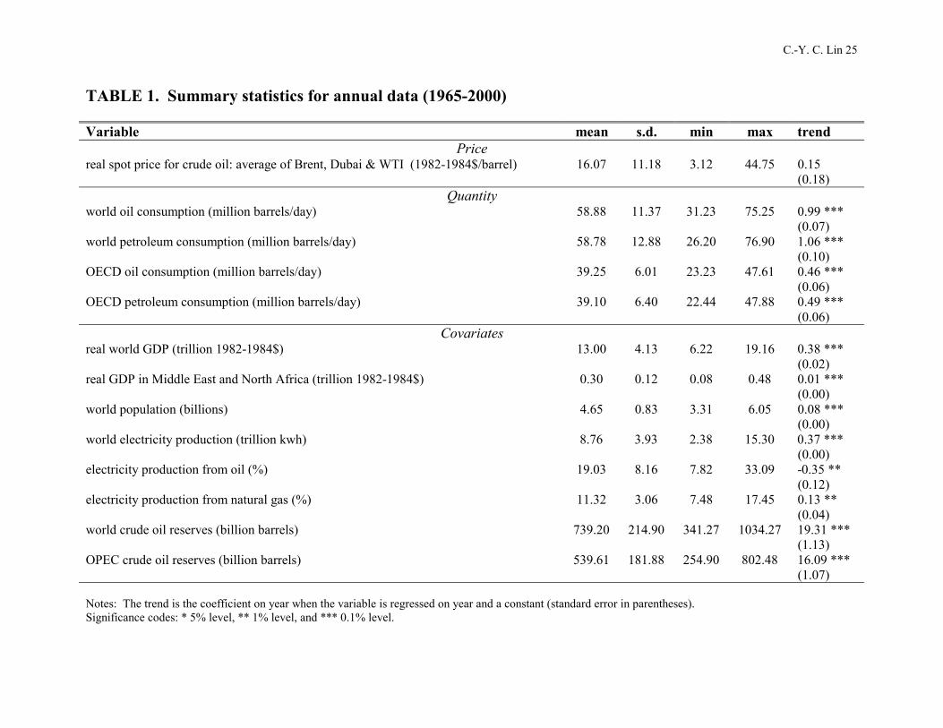
Table 1 provides summary statistics for the variables in my annual data set. For oil price tp , I use the real

annual spot price for crude oil, averaged over the Brent, Dubai, and West Texas Intermediate (WTI) prices. This 4 Although the 2SLS estimates are consistent, they are still biased. No method for obtaining unbiased estimates of the structural parameters exists (Goldberger, 1991, p. 343). 5 Since 2SLS does not fully use all the available information to potentially enhance the efficiency of its estimates, it is sometimes referred to as “limited information estimation” (Ruud, 2000). 6 For this reason, 3SLS is sometimes referred to as “full information estimation” (Ruud, 2000).

C.-Y. C. Lin 10

average price time series was obtained from the World Bank and deflated to 1982-1984 U.S. dollars using the

consumer price index (CPI).

For oil quantity tq , I use two possible measures: world oil consumption as reported by BP and world

petroleum consumption as reported by the U.S. Department of Energy. For comparison, summary statistics are also

provided for oil and petroleum consumption aggregated over only those countries in the Organization for Economic

Cooperation and Development (OECD).

For covariates tx , I use data on the following variables: real world gross domestic product (GDP), real GDP

for the Middle East and North Africa, population, total electricity production, electricity production from oil,

electricity production from gas, world oil reserves, and Organization of Petroleum Exporting Countries (OPEC) oil

reserves. GDP, population and electricity production data were obtained from the World Bank Group World

Development Indicators (WDI) online database. Reserve data were obtained from the Oil and Gas Journal. GDP

data were deflated to 1982-1984 U.S. dollars using the CPI.

As can be seen in the last column of Table 1, most variables exhibit a significant positive trend over 1965-

2000, with two exceptions. The first exception is oil price, which has no significant trend. The trendless nature of

oil price over time is in accordance with many empirical studies (see Krautkraemer, 1998, & references therein).7

The second exception is the percent electricity production from oil, which has a significant downward trend. While

the electricity production from oil is declining, however, that from natural gas is increasing. Over the period 1965-

2000, the world thus appears to be substituting away from oil and towards natural gas as its source of electricity.

Table 2 presents the correlations among my two measures of world quantity and their OECD analogs. Oil

consumption and petroleum consumption are highly correlated both for the world and for the OECD; moreover, the

world aggregates are highly correlated with the OECD aggregates as well.

Figure 1 plots the time series for price and for the various measures of quantity. Once again, my various

measures of quantity are highly correlated and upward-sloping. The real oil price jumps in 1974 and again in 1979,

and drops in 1986, in accordance with historical developments in the world oil market (Yergin, 1992).

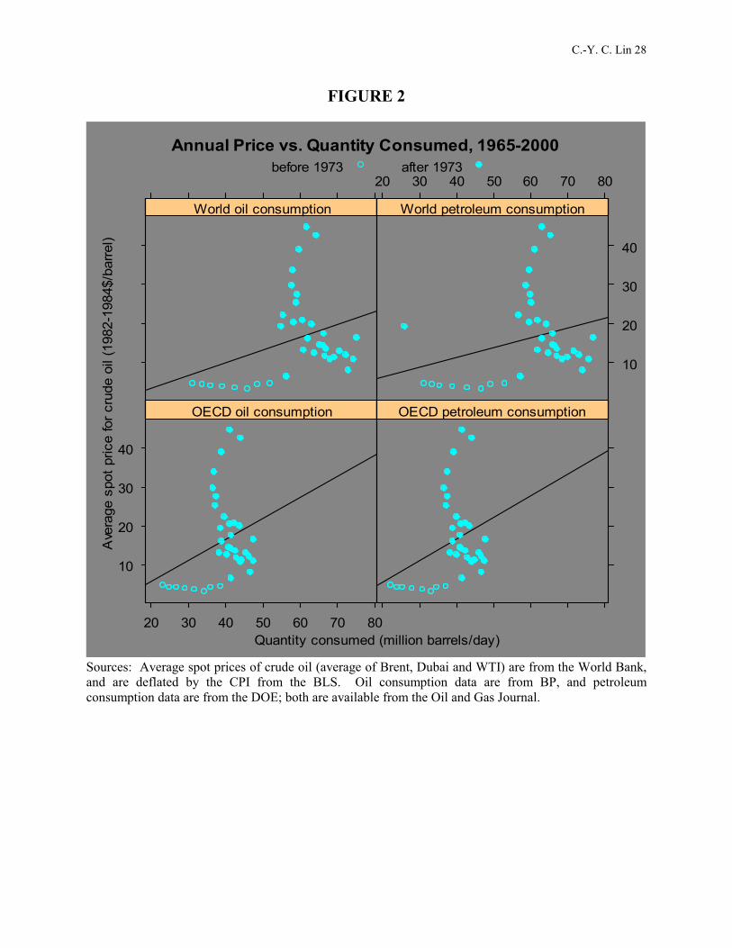
Figure 2 presents scatter plots of price versus each of the measures of quantity. The least-squares

regression line is plotted as well. Observations before the 1973 Arab oil embargo are denoted with an open circle;

7 In addition to oil supply and demand, the trendless nature of oil prices is yet another aspect of the oil market that continues to puzzle economists. See Lin (2004a) and Lin (2004b) for theoretical expositions of the latter empirical puzzle and attempts to rationalize the puzzle with theory.

C.-Y. C. Lin 11

observations from 1973 onwards are denoted with a filled circle. Several features of these plots should be noted.

First, the least-squares regression line has a positive slope. Second, this least-squares regression line is neither the

supply function nor the demand function. Since the prices and quantities are observations of equilibrium

transactions, it is impossible to identify either supply or demand: this is precisely the simultaneity problem

described in Section 2. The third feature to note is that observations that took place before the 1973 oil embargo

appear markedly different from those that took place after it. In particular, when compared with the pre-1973

market, the post-1973 market had higher prices and quantities. Moreover, while quantities varied more than price

before 1973, prices varied more than quantity after 1973.

Figure 3 is directly analogous to Figure 2, except that the prices and quantities used for the scatter plots are

in logs rather than in levels. The qualitative features of the scatter plots of price versus quantity appear robust to

whether these variables are logged or not.

Since the data used to measure oil quantity in my annual data set were consumption data, one may wonder

whether using production rather than consumption as a measure of quantity might yield different results. Although I

was unable to obtain data for either oil or petroleum production that spanned the years 1965-2000,8 my monthly data

does include a series on world oil production that spans 1970-2003. In order to compare measures of consumption

with those of production, I compare my annual consumption time series with an annual average of my monthly

production time series.9 As seen in Figure 4, oil consumption and oil production are highly correlated, with a

correlation of 0.94. Thus, my results should be robust to whether I use consumption or production as my measure of

quantity.

Having described my annual data set, I now turn to my monthly data set.

4.2 Monthly Data (1981-2000)

While my monthly data covers fewer years than my annual data set, it has several advantages.10 First, there

are many more observations in my monthly data set than in my annual data set, which increases the number of

degrees of freedom in my estimations. Second, my monthly data set includes many more variables than my annual

8 I did obtain data on annual world petroleum production, but the data only spans 1973-1991. Because this data had so few observations, I did not use it for my annual analyses. 9 Averaging over the months for each year is more appropriate than summing because monthly production is reported as a rate: million barrels per day. 10 I chose the period length to optimally trade off the number of observations I could use with the number of variables with data available for the entire length of that period.

C.-Y. C. Lin 12

data set does. Third, all the observations in my monthly data set took place after the 1973 Arab oil embargo. As

seen in the previous section, the oil market appeared to have changed dramatically after 1973. My monthly data

thus enables me to focus on the post-1973 oil market.

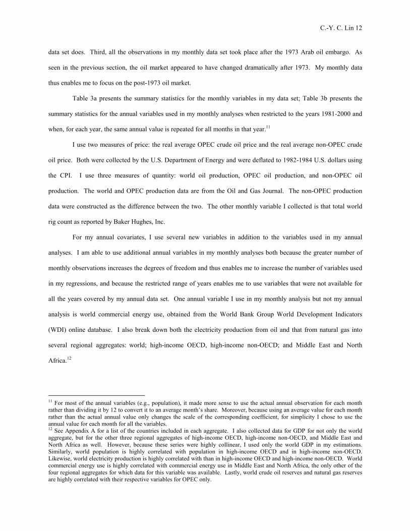
Table 3a presents the summary statistics for the monthly variables in my data set; Table 3b presents the

summary statistics for the annual variables used in my monthly analyses when restricted to the years 1981-2000 and

when, for each year, the same annual value is repeated for all months in that year.11

I use two measures of price: the real average OPEC crude oil price and the real average non-OPEC crude

oil price. Both were collected by the U.S. Department of Energy and were deflated to 1982-1984 U.S. dollars using

the CPI. I use three measures of quantity: world oil production, OPEC oil production, and non-OPEC oil

production. The world and OPEC production data are from the Oil and Gas Journal. The non-OPEC production

data were constructed as the difference between the two. The other monthly variable I collected is that total world

rig count as reported by Baker Hughes, Inc.

For my annual covariates, I use several new variables in addition to the variables used in my annual

analyses. I am able to use additional annual variables in my monthly analyses both because the greater number of

monthly observations increases the degrees of freedom and thus enables me to increase the number of variables used

in my regressions, and because the restricted range of years enables me to use variables that were not available for

all the years covered by my annual data set. One annual variable I use in my monthly analysis but not my annual

analysis is world commercial energy use, obtained from the World Bank Group World Development Indicators

(WDI) online database. I also break down both the electricity production from oil and that from natural gas into

several regional aggregates: world; high-income OECD, high-income non-OECD; and Middle East and North

Africa.12

11 For most of the annual variables (e.g., population), it made more sense to use the actual annual observation for each month rather than dividing it by 12 to convert it to an average month’s share. Moreover, because using an average value for each month rather than the actual annual value only changes the scale of the corresponding coefficient, for simplicity I chose to use the annual value for each month for all the variables. 12 See Appendix A for a list of the countries included in each aggregate. I also collected data for GDP for not only the world aggregate, but for the other three regional aggregates of high-income OECD, high-income non-OECD, and Middle East and North Africa as well. However, because these series were highly collinear, I used only the world GDP in my estimations. Similarly, world population is highly correlated with population in high-income OECD and in high-income non-OECD. Likewise, world electricity production is highly correlated with than in high-income OECD and high-income non-OECD. World commercial energy use is highly correlated with commercial energy use in Middle East and North Africa, the only other of the four regional aggregates for which data for this variable was available. Lastly, world crude oil reserves and natural gas reserves are highly correlated with their respective variables for OPEC only.

C.-Y. C. Lin 13

Unlike for the annual time series, monthly oil price has a significant negative trend over 1981-2000.

Production has a significant positive trend. World rig count is declining. The signs of the trends for the annual

variables when converted to a monthly series and restricted to 1981-2000 are similar to the analogous variables in

the annual data set. One exception is real GDP in the Middle East and North Africa, which now has a significant

negative trend. As for the new annual variables, world commercial energy use has a significant positive trend, and

electricity production from oil and that from gas in different parts of the world all have trends of the same sign as the

world aggregate: as in the annual data spanning 1965-2000, electricity production from oil is decreasing while that

from natural gas is increasing in the monthly data spanning 1981-2000.

How correlated are my different measures of price, and how correlated are my different measures of

quantity, both over 1981-2000? My two measures of price, OPEC oil price and non-OPEC oil price, are highly

correlated, with a correlation of 0.99. Table 4 presents the correlation between my various measures of quantity.

While world oil production and OPEC oil production are highly correlated with each other, non-OPEC oil

production is not highly correlated with either of the two.

Figure 5 presents the time series for the various measures of price and quantity. Once again, over the 1981-

2000 time period, OPEC quantity and world quantity are highly correlated and all three measures of quantity are

increasing. OPEC and non-OPEC prices are also correlated over this time period, but are declining. As expected,

prices collapse in the mid-1980s.

Figure 6 displays a scatter plot of the following combinations of price and quantity that I will later use for

my supply and demand estimations: (1) OPEC price and world quantity; (2) OPEC price and OPEC quantity; (3)

non-OPEC price and world quantity; and (4) non-OPEC price and non-OPEC quantity. As before, because these

prices and quantities are equilibrium observations, one cannot identify either a supply curve or a demand curve.

However, unlike before, the least-squares regression line now has a negative rather than a positive slope. Figure 7

plots the analogous scatter plots using logs rather than levels. Because the qualitative features of the plots are the

same whether the variables are in logs or in levels, I will only present the complete results for the levels form for the

estimations; for the logarithmic form, only the results from the efficient and identified 3SLS estimation will be

presented.

Having described my annual and monthly data sets, I now proceed to estimating world oil demand and

supply.

C.-Y. C. Lin 14

5 Results

5.1 Annual Supply and Demand (1965-2000)

For my annual analyses, I make the following exclusion restrictions:

(1) The following covariates are exogenous annual demand shifters dtx that affect the demand for

oil but not its supply: world GDP, population, electricity production, electricity production

from oil, and electricity production from gas.

(2) The following covariates are exogenous annual supply shifters stx that affect the supply of oil

but not its demand: world oil reserves and OPEC oil reserves.

(3) The following covariates ntx are endogenous: GDP in the Middle East and North Africa,

which I assume affects the supply of oil but not its demand.

(4) The following covariates are exogenous market controls ctx that affect both supply and

demand: an indicator variable for year of the 1973 Arab oil embargo and an indicator

variable for all years from 1973 onwards.

All the exogenous covariates ( ), ,d s ct t t tz x x x= will be used as instruments in my instrumental variables estimations.

Table 5 presents the estimates of the reduced-form relationships (4) and (5) between price and quantity,

respectively, and all the covariates. In the price equations, GDP in the Middle East and North Africa has a

significant positive coefficient.13 Moreover, population and electricity production from oil both have a significant

negative coefficient in the log price regression, as does the dummy variable for the year of the Arab oil embargo.

Log prices were higher after the oil embargo.

For the reduced-form quantity regressions, world GDP, population, electricity production from oil and

from gas, and the Arab oil embargo all had a significant positive effect on the quantity of oil consumed. None of the

coefficients in the regressions of petroleum production were individually significant, but altogether they were jointly

significant (p-value = 0.00 in both the level and log regressions).

13 Because GDP in the Middle East and North Africa may be endogenous, I instrument for it in my estimations of the structural demand and supply equations. In the reduced-form regressions, however, I treat it as exogenous.

C.-Y. C. Lin 15

To test whether Assumption 2 that the instruments are correlated with price appears reasonable, I regress

price on the instruments ( ), ,d s ct t t tz x x x= . The results are provided in Table 6. The difference between the

regressions in Table 6 and the analogous price regressions in Table 5 is that the former no longer includes the

endogenous covariate GDP in the Middle East and North Africa as a regressor. In the regression of oil price level,

none of the instruments has a significant coefficient, although altogether they are jointly significant (p-value = 0.00)

and the supply shifters are jointly significant at a 10% level (p-value = 0.06). When log oil price is used, only the

market controls are individually significant, although all the instruments together are jointly significant (p-value =

0.00) and the supply shifters are jointly significant at a 10% level (p-value = 0.07). Because the supply shifters are

jointly significant while the demand shifters are not, one expects the demand equation to be better identified than the

supply equation. However, because neither set of shifters is jointly significant at a 5% level, identification of either

equation may be weak at best.14

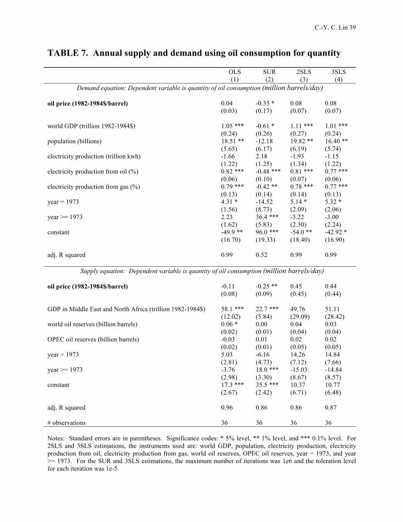
Table 7 presents the results of the structural estimation of the demand and supply equations using oil

consumption as a measure of quantity. As explained above, assuming that my instruments are valid, the OLS results

are neither identified nor efficient, the SUR results are efficient but not identified, the equation-by-equation 2SLS

results are identified but not efficient, and the 3SLS results are both identified and efficient. Table 8 presents

analogous results using logs for oil consumption and for oil price instead of levels.

There are several main results to be gleaned from the estimates in Tables 7 and 8 of annual demand and

supply functions using oil consumption as quantity in both levels and logarithmic form, respectively. First, the price

coefficients are only significant for the SUR estimations, in which case they are negative for both the demand and

the supply equations. In contrast, economic theory suggests that the coefficient should be negative in the demand

equation but positive in the supply equation. Second, while the significance and magnitudes vary, the signs on the

coefficients in the levels estimations are generally the same as those for the corresponding log estimations. Third,

GDP in the Middle East and North Africa has a positive effect on supply that is also significant in most

specifications. This result accords well with anecdotal evidence that, for countries in the Middle East, oil production

is closely tied with national economic policy (Bob Tippee, personal communication, January 23, 2004). Fourth, the

signs of the coefficients in the SUR estimation are often the opposite of the signs for the corresponding coefficients

14 Similarly, regressions could be run of the endogenous GDP in the Middle East and North Africa on the instruments to see if the instruments can also be appropriately used for this regressor as well.

C.-Y. C. Lin 16

in the other three regressions. Lastly, for the efficient and consistent 3SLS estimates, the price coefficient is not

significant for either supply or demand in either the levels or log regressions.

Tables 9 and 10 present analogous results for the supply and demand estimation in levels and logarithmic

form, respectively, using petroleum consumption rather than oil consumption as the measure of quantity. For this

case, the coefficient on price is not significant for either supply or demand in any of the specifications.

Thus, for my annual analyses, although 3SLS should yield efficiently identified price coefficients that are

consistent with economic theory if my econometric and theoretical assumptions hold, it does not. One possible

reason is that my instruments are too weak because they are not adequately correlated with price. Another is that my

maintained assumption of a static and perfectly competitive world oil market is incorrect. Because the results of the

regressions of price on instruments in Table 6 show a weak correlation, the first explanation seems plausible.

To determine whether better instruments can yield estimates of supply and demand curves consistent with a

static and perfectly competitive world market, I now run analogous analyses with my more comprehensive monthly

data.

5.2 Monthly Supply and Demand (1981-2000)

For my monthly analyses, I make the following exclusion restrictions:

(1) The following covariates are exogenous demand shifters dtx that affect the demand for oil but not

its supply: world GDP; world population; world commercial energy use; world electricity production;

electricity production from oil in the world, in high-income OECD countries, in high-income non-

OECD countries, and in the Middle East and North Africa; electricity production from gas in the

world, in high-income OECD countries, in high-income non-OECD countries, and in the Middle East

and North Africa; and world natural gas reserves.

(2) The following covariates are exogenous supply shifters stx that affect the supply of oil but not its

demand: total world rig count and world oil reserves.

(3) The following covariates ntx are endogenous: GDP in the Middle East and North Africa, which I

assume affects the supply of oil but not its demand.

C.-Y. C. Lin 17

(4) The following covariates are exogenous market controls ctx that affect both supply and demand:

an indicator variable for the summer months (June, July and August), and an indicator variable for the

winter months (December, January and February).15

All the exogenous covariates ( ), ,d s ct t t tz x x x= will be used as instruments in my instrumental variables estimations.

Tables 11a and 11b present the estimates of the reduced-form relationships (4) and (5) between price of oil

and quantity of oil production, respectively, and all the covariates. For the reduced-form price regressions, the signs

of the significant coefficients appear to be robust to whether or not the price is the OPEC price or the non-OPEC

price, and to whether or not the price is logged. Among the covariates with a positive effect on price are the total

world rig count, GDP in the Middle East and North Africa, 16 world electricity production, electricity production

from natural gas in high-income OECD countries, and world oil reserves. Among the covariates with a negative

effect on price are world population, world commercial energy use, electricity production from oil in the Middle

East and North Africa, and electricity production from natural gas in high-income non-OECD countries.

For the reduced-form quantity regressions, more coefficients are significant in the regressions of non-

OPEC oil production than in those of world or OPEC oil production. For world production, world commercial

energy use, electricity production from oil in high-income OECD countries, and electricity from gas in high-income

non-OECD countries all have a significant positive effect on world oil production, while electricity production from

gas in high-income OECD countries has a significant negative effect.

To test whether Assumption 2 that the instruments are correlated with price appears reasonable, I regress

price on the instruments ( ), ,d s ct t t tz x x x= . The results are provided in Table 12. The difference between the

regressions in Table 12 and the analogous price regressions in Table 11a is that the former no longer includes the

endogenous covariate GDP in the Middle East and North Africa as a regressor. Unlike in the annual analyses, the

instruments used in my monthly analyses appear to be highly correlated with price. Not only are all the instruments

together jointly significant (p-value = 0.00 in all regressions), but the demand shifters and supply shifters are

significant as well. Thus, my instruments appear not only credible, but also strong as well.

15 The year of the monthly market was too highly correlated with some of the annual covariates to be included as an additional market control. 16 Because GDP in the Middle East and North Africa may be endogenous, I instrument for it in my estimations of the structural demand and supply equations. In the reduced-form regressions, however, I treat it as exogenous.

C.-Y. C. Lin 18

The demand shifters that have a significant positive effect on price are world electricity production and

electricity production from natural gas in high-income OECD countries. The demand shifters that have a significant

negative effect on price are population, commercial energy use, electricity production from oil in the world and in

the Middle East and North Africa, and electricity production from natural gas in the world, in high-income non-

OECD countries, and in the Middle East and North Africa. The demand shifters are jointly significant (p-value =

0.00 in all regressions). Because many demand shifters are individually significant, and because they are together

jointly significant, the supply equation should be identified when these shifters are used as instruments.

For the supply shifters, the rig count and world oil reserves both have significant positive effects on price.

These signs seem reasonable, as rig counts and world oil reserves should both shift the supply curve upward. The

supply shifters are jointly significant (p-value = 0.00 in all regressions). Because the supply shifters are individually

and jointly significant, the demand equation should be identified when these shifters are used as instruments.

Thus, Assumption 2 that the instruments are correlated with price appears to hold, and the use of these

instruments should yield identification.17 As a consequence, if the estimates of supply and demand arising from

instrumental variables techniques are not consistent with a simple theoretical model of a static and perfectly

competitive world oil market, the fault is likely to lie in the theoretical assumptions themselves rather than in its

econometric estimation.

Tables 13a and 13b present the estimates for demand and supply, respectively, when the price variable is

the OPEC oil price and the quantity variable is world oil production. Analogous results are presented for OPEC oil

price and OPEC oil production in Tables 14a-b; non-OPEC oil price and world oil production in Tables 15a-b; and

non-OPEC oil price and non-OPEC oil production in Tables 16a-b.

For the estimates of demand, economic theory predicts that price should have a negative effect on demand,

and econometric theory predicts that, if the theoretical model is correct, properly instrumenting for price will yield

identified price coefficients of the appropriate sign. However, as seen in Tables 13a-16a, while the price coefficient

is significantly negative in all of the (non-instrumented) OLS and SUR specifications for all the price-quantity

combinations used, once instruments are added in 2SLS, the coefficients, while still negative, are no longer

significant. Moreover, for the (instrumented) 3SLS estimations, which should yield coefficients that are both

identified and efficient, the price coefficient is significantly positive in the regression of OPEC oil demand on OPEC

17 Similarly, regressions could be run of the endogenous GDP in the Middle East and North Africa on the instruments to see if the instruments can also be appropriately used for this regressor as well.

C.-Y. C. Lin 19

price, although it is significantly negative in the regression of non-OPEC oil demand on non-OPEC price and not

significant at a 5% level in the regressions of world oil demand on either OPEC or non-OPEC price. World oil

demand therefore appears inelastic to oil price, OPEC or otherwise. Moreover, while world oil demand and non-

OPEC oil demand are consistent with a static and perfectly competitive world oil market, OPEC oil demand is not.

For the estimates of supply, on the other hand, economic theory predicts that price should have a positive

effect on demand, and econometric theory predicts that, if the theoretical model is correct, properly instrumenting

for price will yield identified price coefficients of the appropriate sign. As expected, the price coefficient has the

wrong sign in the (non-instrumented) OLS and SUR specifications for all the price-quantity combinations in Tables

13b-16b. Using instruments for price and for GDP in the Middle East and North Africa does not yield a

significantly positive price coefficient in any of the 2SLS or 3SLS specifications, although in some cases it yields

coefficients that are no longer significantly negative. In particular, the use of instruments yields an OPEC supply

curve that is inelastic to OPEC price. Thus, while OPEC supply is consistent with a static and perfectly competitive

oil market, both world supply and non-OPEC supply are not.

For any given combination of price and quantity, the signs of the significant coefficients on the covariates

tend to be robust across the different estimation methods used (OLS, SUR, 2SLS, and 3SLS). However, for the

3SLS results, the signs are not robust across the different price-quantity combinations: while the signs are similar in

the 3SLS estimations using OPEC price and world quantity; OPEC price and OPEC quantity; and non-OPEC price

and world quantity, the signs are often flipped in the 3SLS estimations using non-OPEC price and non-OPEC

quantity. For example, world population, world commercial energy use, electricity production from oil in the

Middle East and North Africa, and electricity production from natural gas in the Middle East and North Africa all

have significant positive effects on demand in all price-quantity combinations except that of non-OPEC price and

non-OPEC quantity, in which case the effects are significantly negative. Similarly, electricity production from

natural gas in high-income OECD countries has a negative effect in all price-quantity combinations except that of

non-OPEC price and non-OPEC quantity, in which case the effect is significantly positive. For the 3SLS estimates

of supply, world crude oil reserves has a significant positive effect on supply in all price-quantity combinations

except that of non-OPEC price and non-OPEC quantity, in which case the effects are significantly negative.

Many of the signs of the 3SLS coefficients on the covariates in the demand equations that are robust with

respect to the price-quantity combination used appear realistic. For example, electricity production from oil both in

C.-Y. C. Lin 20

high-income OECD countries and in high-income non-OECD countries has a positive effect on oil demand. This is

reasonable, as the more oil is needed for electricity, the higher should be oil demand. The stock of natural gas

reserves has a negative effect on demand, which again is reasonable because natural gas is a substitute for oil.18 One

potentially surprising result is that world GDP has a negative effect on demand, which suggests that, controlling for

such covariates as energy use and electricity production, oil is an inferior good, perhaps because a richer world

economy would use oil more efficiently.

The signs on the 3SLS coefficients in the supply equation appear realistic as well. For example, total rig

count has a positive effect on supply, since, all else equal, the more exploration and production there is that takes

place, the more oil there is to supply. GDP in the Middle East and North Africa has a positive effect on supply.

Except in the regression of non-OPEC supply on non-OPEC price, the stock of crude oil reserves has a positive

effect on supply, as expected.

Do the results change when oil prices and quantities are logged? The 3SLS results for estimates of demand

and supply for the various price-quantity combinations when prices and quantities are in logs rather than in levels

are presented in Tables 17a and 17b, respectively. For the most part, the qualitative results from 3SLS appear robust

to whether the equations are in levels or logarithmic form. The main exception is that for the estimates of supply,

the only supply curve that has a non-negative slope consistent with economic theory when the prices and quantities

are logged is non-OPEC supply, not OPEC supply, as was the case when prices and quantities were in levels. Thus,

the previous result that OPEC supply was consistent with theory is not robust to the functional form of the supply

curve. The robust result, therefore, is that for most specifications of supply, the price coefficients are not consistent

with the assumptions of a static and perfectly competitive market.

Because the instruments used in my monthly analyses are both strong and credible, 3SLS yields efficiently

identified price coefficients. Are these coefficients consistent with economic theory? Well, yes and no. Non-OPEC

oil demand does indeed exhibit a negative slope with respect to non-OPEC oil price, while world oil demand is

inelastic to both OPEC price and non-OPEC price. Thus, both non-OPEC and world demand functions are

consistent with economic theory, which predicts that demand should be (weakly) downward-sloping. Moreover,

OPEC supply in levels form appears inelastic to OPEC price, and log non-OPEC supply appears inelastic to log non-

OPEC price, which are both consistent with the theoretical prediction that supply should be (weakly) upward-

18 Ideally, natural gas price should be used as a regressor in the demand equation. As an extension to my work, I can look for appropriate monthly natural gas price data to include in my demand estimation.

C.-Y. C. Lin 21

sloping. However, the 3SLS estimates for OPEC demand (in both levels and logs), OPEC supply (in logs), non-

OPEC supply (in levels), and world supply (in both levels and logs) all yield price coefficients of the wrong sign. It

thus appears that OPEC demand and most specifications for supply do not satisfy the simply theoretical assumptions

of a static perfectly competitive oil market.

6 Conclusion

Is it possible to obtain efficiently identified estimates of aggregate supply and demand curves for world oil

under the assumptions of a static and perfectly competitive world oil market, or is the endeavor doomed to yield a

dry hole? The answer at first blush appears mixed. When annual data spanning 1965-2000 were used, the

instruments chosen, while credible, were weak, and, as a consequence, neither supply nor demand was identified. In

contrast, with monthly data spanning 1981-2000, the instruments chosen were both strong and credible. However,

although the efficiently identified monthly supply and demand curves were consistent with economic theory in the

cases of world demand, non-OPEC demand and two specifications for supply, this was not the case for either OPEC

demand or for most specifications for supply.

That even the use of strong and credible instruments and of joint estimation did not yield price coefficients

of the expected sign for OPEC demand or for most specifications for supply suggests that either my econometric

specification or the underlying economic theory is incorrect.

Is the econometric specification to blame? In addition to my Assumptions 1-3 on the instruments, which

appear to be satisfied for my monthly analyses, another underlying assumption of my econometric model is that both

demand and supply are linear with fixed coefficients and additive errors. This assumption could be relaxed in future

work using methods such as those developed by Angrist et al. (2000), Manski, (1997), and by Newey, Powell and

Vella (1999). To a first-order approximation, however, one would expect that imposing linearity and additivity

should not affect the sign of the price coefficients.

A potentially more devastating culprit for my counter-intuitive results, in addition to the underlying

econometric assumptions of linearity and additivity, is the theory itself. My model of the world oil market assumed

that it was both static and perfectly competitive. However, the oil market is unlikely to be either.

C.-Y. C. Lin 22

The first problematic theoretical assumption is that the oil market consists of static markets isolated in time.

Because oil production is a capital-intensive process involving irreversible investments, and because oil itself is a

nonrenewable resource whose extraction costs are likely to increase over time, the amount of oil supplied at any

point in time is unlikely to be independent of the amount of oil supplied at any other point in time. Indeed, the

Hotelling model of nonrenewable resource extraction predicts that, even if the market were perfectly competitive,

market price would exceed marginal costs, with the difference reflecting the scarcity rent of the resource (Hotelling,

1931). Thus, oil supply is unlikely to be static. To better estimate the supply for oil, a dynamic model is needed.

The second problematic theoretical assumption is that the oil market is perfectly competitive. A more

realistic model would account for the substantial market power exerted by the OPEC oil cartel.

It thus appears that the theoretical assumptions of a static and perfectly competitive market may be

unrealistic, especially in modeling the supply of oil. Indeed, the identified but inefficient 2SLS estimates for

monthly demand all exhibited the appropriate negative sign; the sign for OPEC demand only flipped when OPEC

demand was estimated jointly with OPEC supply in effort to obtain estimates that were not only identified but also

efficient. Had the supply side been more realistically modeled, then joint estimation of demand and supply may not

only have increased the efficiency and significance of the already-negative and identified price coefficients for

demand, but also yielded significant positive price coefficients for supply as well.

Thus, attempting to efficiently identify aggregate oil supply and demand market in the context of a static

and perfectly competitive oil market may indeed be a dry hole. It is a dry hole not because of the non-existence of

either econometric methods or instruments to enable efficient identification, but rather because of the non-

plausibility of the static perfect competition assumptions in the first place. An econometric model that incorporates

either the dynamic or oligopolistic aspects of the oil market, or both, appears to be a more promising prospect for

exploration and development, and one from which richer and more realistic results are likely to be extracted.

C.-Y. C. Lin 23

References

Adelman, M.A. (1962). Natural gas and the world petroleum market. The Journal of Industrial Economics, 10, 76-

112.

Angrist, J., Graddy, K., & Imbens, G.W. (2000). The interpretation of instrumental variables estimators in

simultaneous equations models with an application to the demand for fish. The Review of Economic Studies,

67 (3), 499-527.

Berndt, E.R., & Wood, D.O. (1975). Technology, prices, and the derived demand for energy. The Review of

Economics and Statistics, 57 (3), 259-268.

Gately, D. (1984). A ten-year retrospective: OPEC and the world oil market. Journal of Economic Literature, 22

(3), 1100-1114.

Goldberger, A.S. (1991). A course in econometrics. Cambridge, MA: Harvard University Press.

Hausman, J.A. (1975). Project independence report: an appraisal of U.S. energy needs up to 1985. The Bell

Journal of Economics, 6 (2), 517-551.

Hotelling, H. The economics of exhaustible resources. The Journal of Political Economy, 39 (2), 137-175.

Kennedy, M. An economic model of the world oil market. The Bell Journal of Economics and Management, 5 (2),

540-577.

Krautkraemer, J. (1998). Nonrenewable resource scarcity. Journal of Economic Literature, 36 (4), 2065-2107.

Lin, C.-Y.C. (2004a). Hotelling revisited: Oil prices and endogenous technological progress. Mimeo. Harvard

University.

Lin, C.-Y.C. (2004b). Steady-state growth in a Hotelling model of resource extraction. Mimeo. Harvard

University.

Mankiw, N.G. (1998). Principles of economics. Fort Worth, TX: Dryden Press.

Manski, C.F. (1995). Identification problems in the social sciences. Cambridge, MA: Harvard University Press.

Manski, C.F. (1997). Monotone treatment response. Econometrica, 65 (6), 1311-1334.

Newey, W.K., Powell, J.L., &Vella, F. (1999). Nonparametric estimation of triangular simultaneous equations

models. Econometrica, 67 (3), 565-603.

Nordhaus, W.D., Houthakker, H.S., & Sachs, J.D. (1980). Oil and economic performance in industrial countries.

Brookings Papers on Economic Activity, 1980 (2), 341-399.

C.-Y. C. Lin 24

Oettinger, G.S. (1999). An empirical analysis of the daily labor supply of stadium vendors. The Journal of Political

Economy, 107 (2), 360-392.

R Development Core Team. (2003). R: A language and environment for statistical computing [Computer

programming software]. Vienna, Austria: R Foundation for Statistical Computing. URL: http://www.R-

project.org.

Ruud, P.A. (2000). An introduction to classical econometric theory. Oxford: Oxford University Press.

Yergin, D. (1992). The prize: the epic quest for oil, money, and power. New York: Free Press.

C.-Y. C. Lin 25

TABLE 1. Summary statistics for annual data (1965-2000) Variable mean s.d. min max trend

Price real spot price for crude oil: average of Brent, Dubai & WTI (1982-1984$/barrel) 16.07 11.18 3.12 44.75 0.15

(0.18) Quantity

world oil consumption (million barrels/day) 58.88 11.37 31.23 75.25 0.99 *** (0.07)

world petroleum consumption (million barrels/day) 58.78 12.88 26.20 76.90 1.06 *** (0.10)

OECD oil consumption (million barrels/day) 39.25 6.01 23.23 47.61 0.46 *** (0.06)

OECD petroleum consumption (million barrels/day) 39.10 6.40 22.44 47.88 0.49 *** (0.06)

Covariates real world GDP (trillion 1982-1984$) 13.00 4.13 6.22 19.16 0.38 ***

(0.02) real GDP in Middle East and North Africa (trillion 1982-1984$) 0.30 0.12 0.08 0.48 0.01 ***

(0.00) world population (billions) 4.65 0.83 3.31 6.05 0.08 ***

(0.00) world electricity production (trillion kwh) 8.76 3.93 2.38 15.30 0.37 ***

(0.00) electricity production from oil (%) 19.03 8.16 7.82 33.09 -0.35 **

(0.12) electricity production from natural gas (%) 11.32 3.06 7.48 17.45 0.13 **

(0.04) world crude oil reserves (billion barrels) 739.20 214.90 341.27 1034.27 19.31 ***

(1.13) OPEC crude oil reserves (billion barrels) 539.61 181.88 254.90 802.48 16.09 ***

(1.07) Notes: The trend is the coefficient on year when the variable is regressed on year and a constant (standard error in parentheses). Significance codes: * 5% level, ** 1% level, and *** 0.1% level.

C.-Y. C. Lin 26

TABLE 2. Correlations between various measures of annual quantity oil consumption, world oil consumption, OECD petroleum consumption,

world petroleum consumption, OECD

oil consumption, world 1.00 oil consumption, OECD 0.96 1.00 pet. consumption, world 0.93 0.88 1.00 pet. consumption, OECD 0.97 1.00 0.94 1.00 Note: Consumptions is measured in million barrels/day.

C.-Y. C. Lin 27

FIGURE 1

Annual Price and Quantity Consumed Time Series

Year

Pric

e (1

982-

1984

$/ba

rrel)

or Q

uant

ity c

onsu

med

(m

illio

n ba

rrel

s/da

y)

0

20

40

60

80

1970 1980 1990 2000

OECD oil consumed OECD pet. consumed

1970 1980 1990 2000

Spot price for crude oil

World oil consumed World pet. consumed

1970 1980 1990 2000

Sources: Average spot prices of crude oil (average of Brent, Dubai and WTI) are from the World Bank, and are deflated by the CPI from the BLS. Oil consumption data are from BP, and petroleum consumption data are from the DOE; both are available from the Oil and Gas Journal.

C.-Y. C. Lin 28

FIGURE 2

Annual Price vs. Quantity Consumed, 1965-2000

Quantity consumed (million barrels/day)

Ave

rage

spo

t pric

e fo

r cru

de o

il (1

982-

1984

$/ba

rrel)

10

20

30

40

20 30 40 50 60 70 80

OECD oil consumption OECD petroleum consumption

World oil consumption

10

20

30

40

World petroleum consumption

20 30 40 50 60 70 80before 1973 after 1973

Sources: Average spot prices of crude oil (average of Brent, Dubai and WTI) are from the World Bank, and are deflated by the CPI from the BLS. Oil consumption data are from BP, and petroleum consumption data are from the DOE; both are available from the Oil and Gas Journal.

C.-Y. C. Lin 29

FIGURE 3

Annual ln(Price) vs. ln(Quantity Consumed), 1965-2000

ln(Quantity consumed (million barrels/day))

ln(A

vera

ge s

pot p

rice

for c

rude

oil

(198

2-19

84$/

barre

l))

1.0

1.5

2.0

2.5

3.0

3.5

3.5 4.0

OECD oil consumption OECD petroleum consumption

World oil consumption

1.0

1.5

2.0

2.5

3.0

3.5

World petroleum consumption

3.5 4.0before 1973 after 1973

Sources: Average spot prices of crude oil (average of Brent, Dubai and WTI) are from the World Bank, and are deflated by the CPI from the BLS. Oil consumption data are from BP, and petroleum consumption data are from the DOE; both are available from the Oil and Gas Journal.

C.-Y. C. Lin 30

FIGURE 4

Annual World Oil Consumption and Production

correlation = 0.94Year

Oil

Qua

ntity

(mill

ion

barre

ls/d

ay)

30

40

50

60

70

1970 1980 1990 2000

ConsumptionProduction

Years used for annual data (1965-2000)Years used for monthly data (1981-2000)

Sources: Oil consumption data are collected by BP and are available from the Oil and Gas Journal. Oil production data is the annual average of a monthly time series from the Oil and Gas Journal.

C.-Y. C. Lin 31

TABLE 3a. Summary statistics for monthly data (1981-2000): monthly variables Variable mean s.d. min max trend

Price real average spot price for crude oil: total OPEC (1982-1984$/barrel) 17.02 9.00 5.91 39.72 -0.10 ***

(0.01) real average spot price for crude oil: total non-OPEC (1982-1984$/barrel) 17.28 8.82 5.75 43.94 -0.10 ***

(0.01) Quantity

world oil production (million barrels/day) 59.40 4.48 49.39 69.32 0.06 *** (0.00)

OPEC oil production (million barrels/day) 22.50 3.93 13.90 29.59 0.05 *** (0.00)

non-OPEC oil production (million barrels/day) 36.89 1.52 33.17 40.86 0.011 *** (0.001)

Monthly Covariates total world rig count (100 rigs) 25.02 11.71 11.56 62.31 -0.13 ***

(0.01) Notes: The trend is the coefficient on month when the variable is regressed on month and a constant (standard error in parentheses). Significance codes: * 5% level, ** 1% level, and *** 0.1% level.

C.-Y. C. Lin 32

TABLE 3b. Summary statistics for monthly data (1981-2000): Annual covariates

Variable mean s.d. min max trend Annual Covariates

real world GDP (trillion 1982-1984$) 15.77 2.76 11.36 19.16 0.04 *** (0.00)

real GDP in Middle East and North Africa (trillion 1982-1984$) 0.35 0.04 0.30 0.42 -2e-4 *** (0.0000)

world population (billions) 5.28 0.48 4.50 6.05 0.007 *** (0.000)

world commercial energy use (million kt of oil equivalent) 8.53 0.86 7.10 9.94 0.01 *** (0.00)

world electricity production (trillion kwh) 11.70 2.08 8.39 15.30 0.03 *** (0.00)

electricity production from oil, world (%) 15.84 6.74 7.82 27.09 -0.09 *** (0.00)

electricity production from oil, high-income OECD (%) 8.62 2.35 5.40 15.24 -0.03 *** (0.00)

electricity production from oil, high-income non-OECD (%) 32.08 10.08 25.41 62.18 -0.10 *** (0.01)

electricity production from oil, Middle East and North Africa (%) 51.40 5.05 42.32 60.16 -0.06 *** (0.00)

electricity production from natural gas, world (%) 11.86 3.70 7.48 17.45 0.05 *** (0.00)

electricity production from natural gas, high-income OECD (%) 11.30 2.06 8.70 15.72 0.03 *** (0.00)

electricity production from natural gas, high-income non-OECD (%) 18.86 2.86 14.14 24.13 0.03 *** (0.00)

electricity production from natural gas, Middle East and North Africa (%) 37.28 6.96 27.90 49.90 0.10 *** (0.00)

world crude oil reserves (billion barrels) 881.68 152.95 648.53 1034.27 2.00 *** (0.06)

world natural gas reserves (1015 cubic feet) 4.14 0.83 2.63 5.15 0.012 *** (0.0002)

Notes: For the annual covariates, each annual value is repeated for all twelve months in the corresponding year. The trend is the coefficient on year when the variable is regressed on year and a constant (standard error in parentheses). Significance codes: * 5% level, ** 1% level, and *** 0.1% level.

C.-Y. C. Lin 33

TABLE 4. Correlation between various measures of monthly oil quantity world oil production OPEC oil production non-OPEC oil production world oil production 1.00 OPEC oil production 0.94 1.00 non-OPEC oil production 0.51 0.20 1.00 Note: Production is measured in million barrels/day.

C.-Y. C. Lin 34

FIGURE 5

Monthly Price and Quantity Produced Time Series

Year

Pric

e (1

982-

1984

$/ba

rrel)

or Q

uant

ity p

rodu

ced

(mill

ion

barr

els/

day)

20

40

60

1970 1980 1990 2000

Price, non-OPEC Price, OPEC

Quantity, non-OPEC Quantity, OPEC

1970 1980 1990 2000

20

40

60

Quantity, world

Years used for monthly data (1981-2000)

Sources: Oil price data are collected by the DOE and are available from the Oil and Gas Journal. World and OPEC quantity data are from the Oil and Gas Journal. Non-OPEC quantity data were constructed by the author as the difference between the corresponding world and OPEC series.

C.-Y. C. Lin 35

FIGURE 6

Monthly Oil Price vs. Quantity Produced, 1981-2000

Quantity produced (million barrels/day)

Ave

rage

spo

t pr

ice

for c

rude

oil

(198

2-19

84$/

barre

l)

10

20

30

40

20 30 40 50 60 70

Non-OPEC price, Non-OPEC prodn Non-OPEC price, World prodn

OPEC price, OPEC prodn

10

20

30

40

OPEC price, World prodn

20 30 40 50 60 70

Sources: Oil price data are collected by the DOE and are available from the Oil and Gas Journal. World and OPEC quantity data are from the Oil and Gas Journal. Non-OPEC quantity data were constructed by the author as the difference between the corresponding world and OPEC series.

C.-Y. C. Lin 36

FIGURE 7

Monthly ln(Oil Price) vs. ln(Quantity Produced), 1981-2000

ln(Quantity produced (million barrels/day))

ln(A

vera

ge s

pot p

rice

for c

rude

oil

(198

2-19

84$/

barre

l))

2.0

2.5

3.0

3.5

3.0 3.5 4.0

Non-OPEC price, Non-OPEC prodn Non-OPEC price, World prodn

OPEC price, OPEC prodn

2.0

2.5

3.0

3.5

OPEC price, World prodn

3.0 3.5 4.0

Sources: Oil price data are collected by the DOE and are available from the Oil and Gas Journal. World and OPEC quantity data are from the Oil and Gas Journal. Non-OPEC quantity data were constructed by the author as the difference between the corresponding world and OPEC series.

C.-Y. C. Lin 37

TABLE 5. Reduced form estimates for (1) annual world oil price and (2) annual world oil or petroleum quantity consumed

Dependent variable is: Price Quantity consumed (1.a) (1.b) (2.a) (2.b) (2.c) (2.d) oil price ln(oil price) oil qty ln(oil qty) pet. qty ln(pet. qty) world GDP (trillion 1982-1984$) -0.31

(1.02) -0.05 (0.05)

1.10 ** (0.30)

0.02 ** (0.01)

2.12 (1.41)

0.05 (0.04)

GDP in Middle East and North Africa (trillion 1982-1984$) 183.2 *** (27.75)

6.76 *** (1.22)

10.18 (8.09)

0.23 (0.18)

53.13 (38.19)

1.34 (0.95)

population (billions) -24.63 (23.12)

-2.66 * (1.02)

18.60 * (6.74)

0.61 *** (0.15)

53.46 (31.81)

1.50 (0.79)

electricity production (trillion kwh) -0.74 (4.79)

0.31 (0.21)

-1.94 (1.40)

-0.09 ** (0.03)

-9.04 (6.59)

-0.28 (0.16)

electricity production from oil (%) -0.75 (0.37)

-0.05 ** (0.02)

0.79 *** (0.11)

0.02 *** (0.00)

0.87 (0.51)

0.02 (0.01)

electricity production from gas (%) -0.38 (0.56)

-0.01 (0.02)

0.78 *** (0.16)

0.01 ** (0.00)

-0.02 (0.77)

-0.01 (0.02)

world oil reserves (billion barrels) 0.04 (0.07)

0.00 (0.00)

-0.00 (0.02)

0.00 (0.00)

-0.06 (0.09)

-0.00 (0.00)

OPEC oil reserves (billion barrels) 0.01 (0.08)

-0.00 (0.00)

0.00 (0.02)

-0.00 (0.00)

0.06 (0.11)

0.00 (0.00)

year = 1973 -6.11 (5.30)

-0.86 ** (0.23)

4.44 ** (1.55)

0.09 * (0.03)

14.96 (7.30)

0.35 (0.18)

year >= 1973 -2.59 (6.13)

0.98 ** (0.27)

-2.84 (1.79)

-0.08 (0.04)

-15.70 (8.43)

-0.40 (0.21)

constant 71.60 (66.61)

9.15 ** (2.94)

-50.32 * (19.42)

1.14 (0.44)

-145.68 (91.65)

-1.28 (2.29)

p-value (Prob > F) 0.00 *** 0.00 *** 0.00 *** 0.00 *** 0.00 *** 0.00 *** adj. R squared 0.86 0.94 0.99 0.98 0.81 0.71 # observations 36 36 36 36 36 36 Notes: Standard errors are in parentheses. Significance codes: * 5% level, ** 1% level, and *** 0.1% level. Prob>F is the p-value from F-tests on all the coefficients. Oil price is in 1982-1984$/barrel; oil and petroleum consumption are in million barrels/day.

C.-Y. C. Lin 38

TABLE 6. Effects of instruments on annual world oil price Dependent variable is: (1) (2) oil price ln(oil price)

Demand shifters

world GDP (trillion 1982-1984$) 0.76 (1.64)

-0.01 (0.07)

population (billions) -31.59 (37.51)

-2.92 (1.49)

electricity production (trillion kwh) 7.34 (7.52)

0.61 (0.30)

electricity production from oil (%) 0.17 (0.56)

-0.01 (0.02)

electricity production from gas (%) 1.08 (0.83)

0.04 (0.03)

p-value from joint test of all demand shifters [0.61] [0.41]

Supply shifters world oil reserves (billion barrels) 0.05

(0.11) 0.01

(0.00) OPEC oil reserves (billion barrels) -0.12

(0.12) -0.01

(0.00) p-value from joint test of all supply shifters [0.06] [0.07]

Market controls year = 1973 -15.27

(8.32) -1.20 **

(0.33) year >= 1973 17.68

(8.62) 1.72 ***

(0.24) constant 88.82

(109.10) 9.79 *

(4.29) p-value from joint test of all coefficients (Prob > F) 0.00 *** 0.00 *** adj. R squared 0.64 0.99 # observations 36 36 Notes: Standard errors are in parentheses. Significance codes: * 5% level, ** 1% level, and *** 0.1% level. Prob>F is the p-value from F-tests on all the coefficients. F-tests are also conducted for all the demand shifters and for all the supply shifters. Oil price is in 1982-1984$.

C.-Y. C. Lin 39

TABLE 7. Annual supply and demand using oil consumption for quantity OLS SUR 2SLS 3SLS (1) (2) (3) (4)

Demand equation: Dependent variable is quantity of oil consumption (million barrels/day) oil price (1982-1984$/barrel) 0.04

(0.03) -0.35 * (0.17)

0.08 (0.07)

0.08 (0.07)

world GDP (trillion 1982-1984$) 1.05 ***

(0.24) -0.61 * (0.26)

1.11 *** (0.27)

1.01 *** (0.24)

population (billions) 18.51 ** (5.65)

-12.18 (6.17)

19.82 ** (6.19)

16.40 ** (5.74)

electricity production (trillion kwh) -1.66 (1.22)

2.18 (1.25)

-1.93 (1.34)

-1.15 (1.22)

electricity production from oil (%) 0.82 *** (0.06)

-0.48 *** (0.10)

0.81 *** (0.07)

0.77 *** (0.06)

electricity production from gas (%) 0.79 *** (0.13)

-0.42 ** (0.14)

0.78 *** (0.14)

0.77 *** (0.13)

year = 1973 4.31 * (1.56)

-14.52 (8.73)

5.14 * (2.09)

5.32 * (2.06)

year >= 1973 2.23 (1.62)

36.4 *** (5.83)

-3.22 (2.30)

-3.00 (2.24)

constant -49.9 ** (16.70)

96.0 *** (19.33)

-54.0 ** (18.40)

-42.92 * (16.90)

adj. R squared 0.99 0.52 0.99 0.99

Supply equation: Dependent variable is quantity of oil consumption (million barrels/day) oil price (1982-1984$/barrel) -0.11

(0.08) -0.25 ** (0.09)

0.45 (0.45)

0.44 (0.44)

GDP in Middle East and North Africa (trillion 1982-1984$) 58.1 ***

(12.02) 22.7 *** (5.84)

49.76 (29.09)

51.11 (28.42)

world oil reserves (billion barrels) 0.06 * (0.02)

0.00 (0.01)

0.04 (0.04)

0.03 (0.04)

OPEC oil reserves (billion barrels) -0.03 (0.02)

0.01 (0.01)

0.02 (0.05)

0.02 (0.05)

year = 1973 5.03 (2.81)

-6.16 (4.73)

14.26 (7.12)

14.84 (7.66)

year >= 1973 -3.76 (2.98)

18.0 *** (3.30)

-15.03 (8.67)

-14.84 (8.57)

constant 17.3 *** (2.67)

35.5 *** (2.42)

10.37 (6.71)

10.77 (6.48)

adj. R squared 0.96 0.86 0.86 0.87 # observations 36 36 36 36 Notes: Standard errors are in parentheses. Significance codes: * 5% level, ** 1% level, and *** 0.1% level. For 2SLS and 3SLS estimations, the instruments used are: world GDP, population, electricity production, electricity production from oil, electricity production from gas, world oil reserves, OPEC oil reserves, year = 1973, and year >= 1973. For the SUR and 3SLS estimations, the maximum number of iterations was 1e6 and the toleration level for each iteration was 1e-5.

C.-Y. C. Lin 40

TABLE 8. Annual supply and demand using ln(oil consumption) for quantity OLS SUR 2SLS 3SLS (1) (2) (3) (4)

Demand equation: Dependent variable is ln(quantity of oil consumption) ln(oil price) 0.03

(0.02) -0.16 * (0.07)

0.02 (0.04)

0.06 (0.04)

world GDP (trillion 1982-1984$) 0.02 ***

(0.01) -0.01 * (0.00)

0.02 ** (0.01)

0.02 ** (0.01)

population (billions) 0.75 *** (0.13)

-0.37 ** (0.12)

0.73 *** (0.15)

0.73 *** (0.17)

electricity production (trillion kwh) -0.11 *** (0.03)

0.07 ** (0.02)

-0.11 ** (0.03)

-0.10 * (0.04)

electricity production from oil (%) 0.02 *** (0.00)

-0.01 *** (0.00)

0.02 *** (0.00)

0.02 *** (0.00)

electricity production from gas (%) 0.01*** (0.00)

-0.01 * (0.00)

0.02 *** (0.00)

0.01 * (0.00)

year = 1973 0.11** (0.04)

-0.33 (0.18)

0.10 (0.06)

0.17 * (0.07)

year >= 1973 -0.10 (0.05)

0.87 *** (0.16)

-0.08 (0.09)

-0.14 (0.10)

constant 0.71 (0.39)

5.37 *** (0.41)

0.76 (0.50)

0.85 (0.55)

adj. R squared 0.99 0.53 0.99 0.98

Supply equation: Dependent variable is ln(quantity of oil consumption)

ln(price) -0.05 (0.04)

-0.10 * (0.04)

-0.06 (0.09)

-0.11 (0.09)

GDP in Middle East and North Africa (trillion 1982-1984$) 0.96 ***

(0.24) 0.26 * (0.10)

1.21 *** (0.27)

1.48 *** (0.26)

world oil reserves (billion barrels) 0.002 *** (0.000)

0.00 (0.00)

0.002 *** (0.001)

0.002 ** (0.001)

OPEC oil reserves (billion barrels) -0.002 ** (0.00)

-0.00 (0.00)

-0.002 * (0.001)

-0.00 (0.00)

year = 1973 0.07 (0.07)

-0.16 (0.10)

0.09 (0.12)

0.06 (0.13)

year >= 1973 -0.04 (0.08)

0.47 *** (0.09)

-0.07 (0.16)

-0.00 (0.17)

constant 3.24 *** (0.08)

3.72 *** (0.08)

3.24 *** (0.16)

3.36 *** (0.17)

adj. R squared 0.95 0.84 0.95 0.94 # observations 36 36 36 36 Notes: Standard errors are in parentheses. Significance codes: * 5% level, ** 1% level, and *** 0.1% level. For 2SLS and 3SLS estimations, the instruments used are: world GDP, population, electricity production, electricity production from oil, electricity production from gas, world oil reserves, OPEC oil reserves, year = 1973, and year >= 1973. For the SUR and 3SLS estimations, the maximum number of iterations was 1e6 and the toleration level for each iteration was 1e-5. Oil price is in 1982-1984$/barrel; oil consumption is in million barrels/day.

C.-Y. C. Lin 41

TABLE 9. Annual supply and demand using petroleum consumption for quantity OLS SUR 2SLS 3SLS (1) (2) (3) (4)

Demand equation: Dependent variable is quantity of petroleum consumption oil price (1982-1984$/barrel) 0.28

(0.15) -0.32 (0.19)

0.62 (0.38)

0.40 (0.29)

world GDP (trillion 1982-1984$) 1.73

(1.17) -0.19 (0.12)

2.24 (1.37)

0.42 (0.70)

population (billions) 41.85 (27.47)

-5.70 (2.83)

52.65 (31.79)

20.19 (22.46)

electricity production (trillion kwh) -6.06 (5.94)

1.11 (0.57)

-8.36 (6.86)

-0.29 (4.38)

electricity production from oil (%) 0.71 * (0.31)

-0.08 (0.05)

0.64 (0.34)

0.51 * (0.22)

electricity production from gas (%) -0.05 (0.65)

0.03 (0.07)

-0.16 (0.72)

0.21 (0.53)

year = 1973 14.33 (7.59)

-11.84 (10.47)

21.22 (10.70)

18.34 (9.63)

year >= 1973 -14.02 (7.86)

29.6 *** (5.47)

-22.23 (11.78)

-15.46 (10.28)

constant -122.3 (81.14)

61.6 *** (9.54)

-145.9 (94.45)

-45.00 (63.36)

adj. R squared 0.80 0.42 0.76 0.78

Supply equation: Dependent variable is quantity of petroleum consumption oil price (1982-1984$/barrel) -0.20

(0.21) -0.29 (0.17)

-0.43 (0.64)

-0.36 (0.62)

GDP in Middle East and North Africa (trillion 1982-1984$) 114.3 ***

(30.68) 8.95 (4.85)

138.5 ** (41.16)

129.7 ** (37.92)

world oil reserves (billion barrels) 0.00 (0.05)

-0.01 (0.01)

0.00 (0.06)

0.02 (0.04)

OPEC oil reserves (billion barrels) 0.04 (0.06)

0.01 (0.01)

0.03 (0.07)

0.01 (0.06)

year = 1973 13.60 (7.17)

-9.18 (9.41)

13.10 (10.92)

13.31 (10.82)

year >= 1973 -14.30 (7.61)

24.9 *** (4.98)

-14.67 (12.26)

-15.92 (11.97)

constant 16.11 * (6.85)

41.6 *** (3.57)

17.19 (9.49)

14.62 (8.31)

adj. R squared 0.80 0.53 0.79 0.79 # observations 36 36 36 36 Notes: Standard errors are in parentheses. Significance codes: * 5% level, ** 1% level, and *** 0.1% level. For 2SLS and 3SLS estimations, the instruments used are: world GDP, population, electricity production, electricity production from oil, electricity production from gas, world oil reserves, OPEC oil reserves, year = 1973, and year >= 1973. For the SUR and 3SLS estimations, the maximum number of iterations was 1e6 and the toleration level for each iteration was 1e-5. Oil price is in 1982-1984$/barrel; petroleum consumption is in million barrels/day.

C.-Y. C. Lin 42

TABLE 10. Annual Supply and Demand using ln(Petroleum Consumption) for quantity OLS SUR 2SLS 3SLS (1) (2) (3) (4)

Demand equation: Dependent variable is ln(quantity of petroleum consumption) ln(price) 0.18

(0.09) -0.15 (0.09)

0.27 (0.22)

0.20 (0.17)

world GDP (trillion 1982-1984$) 0.05

(0.03) -0.00 (0.00)

0.01 (0.04)

0.03 (0.02)

population (billions) 1.51 * (0.69)

-0.15 * (0.05)

1.70 (0.83)

1.49 (0.73)

electricity production (trillion kwh) -0.26 (0.15)

0.03 * (0.01)

-0.30 (0.18)

-0.24 (0.15)

electricity production from oil (%) 0.02 * (0.01)

-0.00 * (0.00)

0.02 * (0.01)

0.02 ** (0.1)

electricity production from gas (%) -0.01 (0.02)

0.00 (0.00)

-0.01 (0.02)

-0.01 (0.01)

year = 1973 0.46 * (0.21)

-0.28 (0.24)

0.57 (0.35)

0.48 (0.30)

year >= 1973 -0.57 * (0.25)

0.72 *** (0.17)

-0.73 (0.48)

-0.57 (0.41)

constant -1.60 (2.08)

4.40 *** (0.23)

-2.29 (2.69)

-1.51 (2.30)

adj. R squared 0.72 0.34 0.71 0.71

Supply equation: Dependent variable is ln(quantity of petroleum consumption) ln(price) -0.08

(0.11) -0.14 (0.08)

-0.46 (0.30)

-0.35 (0.27)

GDP in Middle East and North Africa (trillion 1982-1984$) 2.23 **

(0.69) 0.09 (0.08)

2.84 ** (0.93)

2.29 ** (0.76)

world oil reserves (billion barrels) 0.00 (0.00)

-0.00 (0.00)

0.00 (0.00)

0.00 (0.00)

OPEC oil reserves (billion barrels) -0.00 (0.00)

0.00 (0.00)

-0.00 (0.00)

-0.00 (0.00)

year = 1973 0.27 (0.20)

-0.22 (0.22)

-0.13 (0.41)

-0.06 (0.39)

year >= 1973 -0.26 (0.23)

0.63 *** (0.15)

0.30 (0.55)

0.16 (0.51)

constant 3.25 *** (0.24)

3.89 *** (0.14)

3.88 *** (0.56)

3.63 *** (0.48)

adj. R squared 0.69 0.44 0.57 0.61 # observations 36 36 36 36 Notes: Standard errors are in parentheses. Significance codes: * 5% level, ** 1% level, and *** 0.1% level. For 2SLS and 3SLS estimations, the instruments used are: world GDP, population, electricity production, electricity production from oil, electricity production from gas, world oil reserves, OPEC oil reserves, year = 1973, and year >= 1973. For the SUR and 3SLS estimations, the maximum number of iterations was 1e6 and the toleration level for each iteration was 1e-5. Oil price is in 1982-1984$/barrel; petroleum consumption is in million barrels/day.

C.-Y. C. Lin 43

TABLE 11a. Reduced form estimates for monthly oil price (1981-2000)

Dependent variable is: Price ln(Price) (1) (2) (3) (4) OPEC non-OPEC OPEC non-OPEC

Monthly Covariates total world rig count (100 rigs) 0.23 ***

(0.05) 0.19 *** (0.05)

0.015 *** (0.004)

0.015 *** (0.004)

summer dummy (Jun, Jul, Aug) -0.40 (0.35)

-0.48 (0.35)

-0.02 (0.03)

-0.02 (0.02)

winter dummy (Dec, Jan, Feb) -0.10 (0.37)

0.09 (0.37)

-0.02 (0.03)

-0.03 (0.03)

Annual Covariates GDP, world (trillion 1982-1984$) 57.22

(25.21) -0.02 (0.77)

0.15 ** (0.06)

0.11 * (0.05)

GDP, Mid East & N.Afr. (trillion 1982-1984$) 57.22 * (25.21)

36.99 (25.51)

5.76 ** (1.84)

4.57 * (1.81)

population, world (billions) -72.01 *** (13.55)

-87.3 *** (13.71)

-5.92 *** (0.99)

-6.25 *** (0.97)

commercial energy use, world (mill. kt of oil equivalent) -40.14 *** (7.04)

-34.7 *** (7.12)

-2.84 *** (0.51)

-2.78 *** (0.51)

electricity production, world (trillion kwh) 23.86 *** (5.00)

26.62 *** (5.06)

1.72 *** (0.36)

1.89 *** (0.36)

electricity prodn from oil, world (%) -2.48 (1.37)

-3.68 ** (1.39)

-0.04 (0.10)

-0.10 (0.10)

electricity prodn from oil, high-inc OECD (%) -2.02 (1.16)

-0.44 (1.18)

-0.22 ** (0.08)

-0.16 (0.08)

electricity prodn from oil, high-inc non-OECD (%) -0.16 (0.16)

-0.20 (0.17)

-0.02 (0.01)

-0.02 * (0.01)

electricity prodn from oil, Mid East & N.Afr. (%) -2.42 *** (0.69)

-2.63 *** (0.70)

-0.12 * (0.05)

-0.14 ** (0.05)

electricity prodn from natural gas, world (%) -4.93 ** (1.83)

-6.00 ** (1.86)

-0.16 (0.13)

-0.24 (0.13)

electricity prodn from natural gas, high-inc OECD (%) 6.68 *** (1.08)

7.13 *** (1.09)

0.37 *** (0.08)

0.39 *** (0.08)

electricity prodn from natural gas, high-inc non-OECD (%) -1.81 *** (0.39)

-1.48 *** (0.40)

-0.15 *** (0.03)

-0.14 *** (0.03)

electricity prodn from natural gas, Mid East & N.Afr. (%) -1.78 * (0.73)

-2.12 ** (0.74)

-0.06 (0.05)

-0.09 (0.05)

crude oil reserves, world (billion barrels) 0.05 *** (0.01)

0.04 ** (0.01)

0.004 *** (0.001)

0.004 *** (0.001)

natural gas reserves, world (1015 cubic ft) -6.41 (3.75)

-8.32 * (3.79)

-0.18 (0.03)

-0.30 (0.27)

constant 673.5 ***

(106.4) 107.6 *** (107.6)

42.64 *** (7.76)

46.82 *** (7.63)

p-value (Prob > F) 0.00 *** 0.00 *** 0.00 *** 0.00 *** adj. R squared 0.94 0.94 0.89 0.88 # observations 240 240 240 240 Notes: Standard errors are in parentheses. Significance codes: * 5% level, ** 1% level, and *** 0.1% level. Prob>F is the p-value from F-tests on all the coefficients. Oil price is in 1982-1984$/barrel.

C.-Y. C. Lin 44

TABLE 11b. Reduced form estimates for monthly oil quantity produced (1981-2000)

Dependent variable is: Quantity ln(Quantity) (1) (2) (3) (4) (5) (6) world OPEC non-

OPEC world OPEC non-

OPEC Monthly Covariates

total world rig count (100 rigs) 0.04 (0.03)

0.01 (0.03)

0.03 * (0.01)

0.00 (0.00)

0.00 (0.00)

6e-4 (3e-4)

summer dummy (Jun, Jul, Aug) -0.33 (0.21)

-0.03 (0.19)

-0.30 *** (0.08)

-0.01 (0.00)

0.00 (0.01)

-8e-3 *** (2e-3)

winter dummy (Dec, Jan, Feb) 0.08 (0.22)

-0.04 (0.20)

0.12 (0.08)

0.00 (0.00)

-0.00 (0.01)

0.00 (0.00)

Annual Covariates GDP, world (trillion 1982-1984$) -0.74

(0.46) -0.24 (0.41)

-0.50 ** (0.17)

-0.01 (0.01)

0.01 (0.02)

-0.013 ** (0.005)

GDP, Mid East & N.Afr. (tr. 1982-1984$) -12.28 (15.19)

13.99 (13.53)

-26.3 *** (4.65)

-0.15 (0.26)

1.08 (0.68)

-0.70 *** (0.15)

population, world (billions) 0.73 (8.16)

-17.79 * (7.27)

18.5 *** (3.04)

-0.01 (0.14)

-0.86 * (0.37)

0.51 *** (0.08)

commercial energy use, world (m. kt of oil equiv) 8.47 * (4.24)

1.58 (3.78)

6.88 *** (1.58)

0.17 * (0.07)

0.13 (0.19)

0.18 *** (0.04)

electricity production, world (trillion kwh) 2.56 (3.01)

5.19 (2.68)

-2.64 * (1.12)

0.03 (0.05)

0.17 (0.14)

-0.07 * (0.03)

elec. prodn from oil, world (%) -0.31 (0.83)

5.19 (2.68)

-0.66 * (0.31)

-0.00 (0.01)

0.05 (0.04)

-0.02 * (0.01)

elec. prodn from oil, high-inc OECD (%) 1.98 ** (0.70)

1.51 * (0.62)

0.48 (0.26)

0.03 ** (0.01)

0.06 (0.03)

0.02 (0.01)

elec. prodn from oil, high-inc non-OECD (%) 0.02 (0.10)

-0.15 (0.09)

0.17 *** (0.04)

-0.00 (0.00)

-0.010 * (0.004)

0.005 *** (0.001)

elec. prodn from oil, Mid East & N. Afr. (%) 0.30 (0.42)

-0.50 (0.37)

0.79 *** (0.16)

0.01 (0.01)

-0.02 (0.02)

0.02 *** (0.00)

elec. prodn from gas, world (%) 0.20 (1.11)

1.18 (0.99)

-0.98 * (0.41)

0.01 (0.02)

0.10 * (05)

-0.03 * (0.01)

elec. prodn from gas, high-inc OECD (%) -1.82 ** (0.65)

-1.43 * (0.58)

-0.40 (0.24)

-0.03 ** (0.01)

-0.08 ** (0.03)

0.01 (0.01)

elec. prodn from gas, high-inc non-OECD (%) 0.76 ** (0.24)

0.42 * (0.21)

0.34 *** (0.09)

0.01 ** (0.00)

0.02 (0.01)

0.009 *** (0.002)

elec. prodn from gas, Mid East & N.Afr. (%) 0.22 (0.44)

-0.46 (0.39)

0.68 *** (0.16)

0.00 (0.01)

-0.02 (0.02)

0.02 *** (0.00)

crude oil reserves, world (billion barrels) -0.01 (0.01)

0.00 (0.01)

-0.02 *** (0.00)

-0.00 (0.00)

0.00 (0.00)

-5e-4 *** (0.1e-4)

natural gas reserves, world (1015 cubic ft) -2.42 (2.26)

3.59 (2.01)

-6.02 *** (0.84)

-0.03 (0.04)

0.25 * (0.10)

-0.17 *** (0.00)

constant -41.94

(64.08) 45.47 (57.07)

-87.4 *** (23.8)

2.17 (1.12)

2.67 (2.88)

0.19 (0.64)

p-value (Prob > F) 0.00 *** 0.00 *** 0.00 *** 0.00 *** 0.00 *** 0.00 *** adj. R squared 0.91 0.92 0.90 0.91 0.90 0.90 # observations 240 240 240 240 240 240 Notes: Standard errors are in parentheses. Significance codes: * 5% level, ** 1% level, and *** 0.1% level. Prob>F is the p-value from F-tests on all the coefficients. Oil production is in million barrels/day.

C.-Y. C. Lin 45

TABLE 12. Effects of instruments on monthly oil price

Dependent variable is: Price ln(Price) (1) (2) (3) (4) OPEC non-OPEC OPEC non-OPEC

Demand shifters GDP, world (trillion 1982-1984$) -0.50

(0.58) -0.75 (0.58)

0.03 (0.04)

0.02 (0.04)

population, world (billions) -69.63 *** (13.63)

-85.76 *** (13.70)

-5.67 *** (1.00)

-6.06 *** (0.98)

commercial energy use, world (mill. kt of oil equivalent) -39.86 *** (7.11)

-34.50 *** (7.14)

-2.82 *** (0.52)

-2.76 *** (0.51)

electricity production, world (trillion kwh) 28.25 *** (4.67)

29.46 *** (4.68)

2.17 *** (0.34)

2.24 *** (0.34)

electricity prodn from oil, world (%) -5.02 *** (0.80)

-5.33 *** (0.80)

-0.29 *** (0.06)

-0.30 *** (0.06)

electricity prodn from oil, high-inc OECD (%) -0.17 (0.83)

0.76 (0.84)

-0.04 (0.06)

-0.01 (0.06)

electricity prodn from oil, high-inc non-OECD (%) 0.13 (0.10)

-0.01 (0.10)

0.01 (0.01)

-0.00 (0.01)

electricity prodn from oil, Mid East & N. Afr. (%) -1.99 ** (0.67)

-2.35 *** (0.68)

-0.07 (0.05)

-0.10 * (0.05)

electricity prodn from natural gas, world (%) -7.96 *** (1.28)

-7.96 *** (1.28)

-0.47 *** (0.09)

-0.48 *** (0.09)

electricity prodn from natural gas, high-inc OECD (%) 6.85 *** (1.08)

7.24 *** (1.09)

0.39 *** (0.08)

0.40 *** (0.08)

electricity prodn from natural gas, high-inc non-OECD (%) -1.24 *** (0.31)

-1.11 *** (0.31)

-0.09 *** (0.02)

-0.09 *** (0.02)

electricity prodn from natural gas, Mid East & N.Afr. (%) -1.56 * (0.74)

-2.01 ** (0.74)

-0.04 (0.05)

-0.07 (0.05)

natural gas reserves, world (1015 cubic ft) -13.54 *** (2.07)

-12.93 *** (2.08)

-0.89 *** (0.15)

-0.87 *** (0.15)

p-value from joint test of all demand shifters [0.00] *** [0.00] *** [0.00] *** [0.00] ***

Supply shifters total world rig count (100 rigs) 0.22 ***

(0.05) 0.19 *** (0.05)

0.01 4*** (0.004)

0.01 4*** (0.004)

crude oil reserves, world (billion barrels) 0.03 ** (0.01)

0.03 ** (0.01)

0.0012 * (0.0006)

0.0015 * (0.0006)

p-value from joint test of all supply shifters [0.00] *** [0.00] *** [0.00] *** [0.00] ***

Market controls summer dummy (Jun, Jul, Aug) -0.40

(0.35) -0.48 (0.35)

-0.03 (0.03)

-0.03 (0.03)

winter dummy (Dec, Jan, Feb) -0.08 (0.37)

-0.07 (0.37)

-0.02 (0.03)

-0.03 (0.03)

constant 708.1 *** (106.2)

764.1 *** (106.8)

46.13 *** (7.83)

49.59 *** (7.65)

p-value from joint test of all coefficients (Prob > F) 0.00 *** 0.00 *** 0.00 *** 0.00 *** adj. R squared 0.94 0.94 0.88 0.88 # observations 240 240 240 240

Notes: Standard errors are in parentheses. Significance codes: * 5% level, ** 1% level, and *** 0.1% level. Prob>F is the p-value from F-tests on all the coefficients. F-tests are also conducted for all the demand shifters and for all the supply shifters. Oil price is in 1982-1984$/barrel. All covariates are annual values except the total world rig count, the summer dummy and the winter dummy.

C.-Y. C. Lin 46

TABLE 13a. Monthly demand using OPEC oil price and quantity of world oil production

Dependent variable is quantity of world oil production (million barrels/day) OLS SUR 2SLS 3SLS (1) (2) (3) (4)

OPEC oil price (1982-1984$/barrel) -0.12 ***

(0.03) -0.32 *** (0.03)

-0.00 (0.11)

0.03 (0.08)

Monthly Covariates

summer dummy (Jun, Jul, Aug) -0.42 * (0.20)

-0.49 (0.50)

-0.39 (0.22)

-0.32 (0.28)

winter dummy (Dec, Jan, Feb) 0.24 (0.20)

0.30 (0.50)

0.16 (0.22)

0.15 (0.28)

Annual Covariates GDP, world (trillion 1982-1984$) -0.98 **

(0.30) -0.12 * (0.05)

-0.67 (0.37)

-0.90 *** (0.17)

population, world (billions) -14.77 (8.21)

2.49 * (1.03)

-0.80 (12.2)

16.14 * (6.94)

commercial energy use, world (million kt of oil equivalent) 2.62 (3.37)

0.95 (0.54)

6.15 (4.16)

8.06 * (3.33)

electricity production, world (trillion kwh) 6.39 * (2.72)

-0.55 (0.38)

2.33 (3.80)

-1.81 (2.73)

electricity production from oil, world (%) -1.35 ** (0.43)

-0.29 ** (0.09)

-0.23 (0.83)

-1.26 * (0.58)

electricity production from oil, high-inc OECD (%) 1.82 *** (0.36)

0.21 ** (0.08)

1.37 ** (0.47)

1.64 *** (0.21)

electricity production from oil, high-inc non-OECD (%) -0.00 (0.05)

0.06 *** (0.01)

-0.07 (0.07)

0.23 *** (0.04)

electricity production from oil, Mid East & N. Afr. (%) -0.38 (0.24)

0.21 *** (0.05)

-0.30 (0.26)

0.75 *** (0.15)

electricity production from natural gas, world (%) -1.53 * (0.69)

-0.31 * (0.13)

0.06 (1.22)

-1.13 (0.85)

electricity production from natural gas, high-inc OECD (%) 0.21 (0.47)

-0.08 (0.08)

-0.91 (0.84)

-1.15 * (0.58)

electricity production from natural gas, high-inc non-OECD (%) 0.38 ** (0.14)

0.09 *** (0.03)

0.47 ** (0.15)

0.74 *** (0.09)

electricity production from natural gas, Mid East & N.Afr. (%) -0.31 (0.27)

0.16 ** (0.05)

-0.34 (0.28)

0.45 ** (0.15)

natural gas reserves, world (1015 cubic ft) -4.30 *** (1.19)

-0.58 * (0.26)

-1.86 (1.96)

-3.61 * (1.52)

constant 121.7 *

(49.95) 41.21 *** (8.61)

24.90 (79.56)

-88.95 (59.98)

adj. R squared 0.92 0.49 0.91 0.85 # observations 240 240 240 240 Notes: Standard errors are in parentheses. Significance codes: * 5% level, ** 1% level, and *** 0.1% level. For 2SLS and 3SLS estimations, the instruments used are: total world rig count; summer dummy; winter dummy; world GDP; world population; world commercial energy use; world electricity production; electricity production from oil for world, high-income OECD, high-income non-OECD, and Middle East and North Africa; electricity production from natural gas for world, high-income OECD, high-income non-OECD, and Middle East and North Africa; world crude oil reserves; and world natural gas reserves. For the SUR and 3SLS estimations, demand and supply equations corresponding to the same choice of price and quantity variables were estimated jointly, the maximum number of iterations was 1e6, and the toleration level for each iteration was 1e-5.

C.-Y. C. Lin 47

TABLE 13b. Monthly supply using OPEC oil price and quantity of world oil production

Dependent variable is quantity of world oil production (million barrels/day) OLS SUR 2SLS 3SLS (1) (2) (3) (4)

OPEC oil price (1982-1984$/barrel) -0.21 ***

(0.04) -0.31 *** (0.02)

-0.21 *** (0.05)

-0.17 *** (0.03)

Monthly Covariates

total world rig count (100 rigs) 0.09 ** (0.03)

0.012 *** (0.004)

0.08 * (0.04)

0.06 ** (0.02)

summer dummy (Jun, Jul, Aug) -0.41 (0.26)

-0.48 (0.45)

-0.41 (0.26)

-0.40 (0.26)

winter dummy (Dec, Jan, Feb) 0.06 (0.27)

0.27 (0.45)

0.07 (0.27)

0.11 (0.27)

Annual Covariates GDP, Mid East & N.Afr. (trillion 1982-1984$) 48.85 ***

(3.49) 8.77 *** (1.49)

50.52 *** (3.55)

49.96 *** (3.49)

crude oil reserves, world (billion barrels) 0.028 *** (0.001)

0.005 *** (0.001)

0.028 *** (0.001)

0.029 *** (0.001)

constant 18.68 ***

(1.84) 56.56 *** (1.41)

18.05 *** (1.88)

18.02 *** (1.88)

adj. R squared 0.86 0.60 0.86 0.86 # observations 240 240 240 240 Notes: Standard errors are in parentheses. Significance codes: * 5% level, ** 1% level, and *** 0.1% level. For 2SLS and 3SLS estimations, the instruments used are: total world rig count; summer dummy; winter dummy; world GDP; world population; world commercial energy use; world electricity production; electricity production from oil for world, high-income OECD, high-income non-OECD, and Middle East and North Africa; electricity production from natural gas for world, high-income OECD, high-income non-OECD, and Middle East and North Africa; world crude oil reserves; and world natural gas reserves. For the SUR and 3SLS estimations, demand and supply equations corresponding to the same choice of price and quantity variables were estimated jointly, the maximum number of iterations was 1e6, and the toleration level for each iteration was 1e-5.

C.-Y. C. Lin 48

TABLE 14a. Monthly demand using OPEC oil price and quantity of OPEC oil production

Dependent variable is quantity of OPEC oil production (million barrels/day) OLS SUR 2SLS 3SLS (1) (2) (3) (4)

OPEC oil price (1982-1984$/barrel) -0.13 ***

(0.03) -0.19 *** (0.03)

-0.01 (0.10)

0.66 *** (0.16)

Monthly Covariates

summer dummy (Jun, Jul, Aug) -0.09 (0.18)

-0.12 (0.48)

-0.04 (0.19)

0.28 (0.42)

winter dummy (Dec, Jan, Feb) 0.04 (0.18)

0.06 (0.48)

-0.01 (0.19)

-0.29 (0.42)

Annual Covariates GDP, world (trillion 1982-1984$) -0.79 **

(0.27) -0.20 *** (0.06)

-0.57 (0.32)

-0.20 (0.45)

population, world (billions) -27.73 *** (7.38)

5.07 *** (1.10)

-17.96 (10.77)

58.83 *** (16.45)

commercial energy use, world (million kt of oil equivalent) -1.71 (3.03)

1.96 *** (0.57)

0.76 (3.67)

30.16 *** (6.42)

electricity production, world (trillion kwh) 9.50 *** (2.44)

-0.96 * (0.40)

6.66 * (3.35)

-20.14 *** (5.59)

electricity production from oil, world (%) -1.22 ** (0.39)

-0.40 *** (0.10)

-0.44 (0.73)

2.24 (1.16)

electricity production from oil, high-inc OECD (%) 2.22 *** (0.33)

0.29 *** (0.08)

1.90 *** (0.42)

0.88 (0.58)

electricity production from oil, high-inc non-OECD (%) -0.04 (0.05)

0.09 *** (0.01)

-0.09 (0.06)

0.13 (0.09)

electricity production from oil, Mid East & N. Afr. (%) -0.60 ** (0.22)

0.35 *** (0.05)

-0.55 * (0.23)

2.01 *** (0.35)

electricity production from natural gas, world (%) -0.95 (0.62)

-0.48 *** (0.14)

0.16 (1.08)

4.00 * (1.71)

electricity production from natural gas, high-inc OECD (%) -0.29 (0.42)

-0.12 (0.09)

-1.07 (0.75)

-4.87 *** (1.18)

electricity production from natural gas, high-inc non-OECD (%) 0.44 *** (0.12)

0.14 *** (0.03)

0.51 *** (0.13)

1.20 *** (0.20)

electricity production from natural gas, Mid East & N.Afr. (%) -0.55 * (0.24)

0.29 *** (0.06)

-0.58 * (0.25)

1.56 *** (0.37)

natural gas reserves, world (1015 cubic ft) -0.21 (1.07)

-1.47 *** (0.27)

1.49 (1.73)

5.08 (2.90)

constant 147.1 **

(44.93) -20.68 * (9.11)

79.36 (70.21)

-562.8 *** (116.6)

adj. R squared 0.92 0.40 0.91 0.56 # observations 240 240 240 240 Notes: Standard errors are in parentheses. Significance codes: * 5% level, ** 1% level, and *** 0.1% level. For 2SLS and 3SLS estimations, the instruments used are: total world rig count; summer dummy; winter dummy; world GDP; world population; world commercial energy use; world electricity production; electricity production from oil for world, high-income OECD, high-income non-OECD, and Middle East and North Africa; electricity production from natural gas for world, high-income OECD, high-income non-OECD, and Middle East and North Africa; world crude oil reserves; and world natural gas reserves. For the SUR and 3SLS estimations, demand and supply equations corresponding to the same choice of price and quantity variables were estimated jointly, the maximum number of iterations was 1e6, and the toleration level for each iteration was 1e-5.

C.-Y. C. Lin 49

TABLE 14b. Monthly supply using OPEC oil price and quantity of OPEC oil production

Dependent variable is quantity of OPEC oil production OLS SUR 2SLS 3SLS (1) (2) (3) (4)

OPEC oil price (1982-1984$/barrel) -0.11 **

(0.04) -0.19 *** (0.02)

-0.06 (0.05)

-0.07 (0.04)

Monthly Covariates

total world rig count (100 rigs) 0.15 *** (0.03)

0.010 * (0.004)

0.12 *** (0.04)

0.13 *** (0.03)

summer dummy (Jun, Jul, Aug) -0.04 (0.26)

-0.12 (0.42)

-0.02 (0.26)

-0.03 (0.26)

winter dummy (Dec, Jan, Feb) -0.31 (0.26)

0.04 (0.42)

-0.26 (0.27)

-0.28 (0.26)

Annual Covariates GDP, Mid East & N.Afr. (trillion 1982-1984$) 29.82 ***

(3.42) 12.19 *** (1.53)

29.87 *** (3.50)

30.11 *** (3.46)

crude oil reserves, world (billion barrels) 0.031 *** (0.001)

0.008 *** (0.001)

0.031 *** (0.001)

0.031 *** (0.001)

constant -17.00 ***

(1.81) 14.20 *** (1.43)

-17.48 *** (1.85)

-17.47 *** (1.85)

adj. R squared 0.83 0.54 0.83 0.83 # observations 240 240 240 240 Notes: Standard errors are in parentheses. Significance codes: * 5% level, ** 1% level, and *** 0.1% level. For 2SLS and 3SLS estimations, the instruments used are: total world rig count; summer dummy; winter dummy; world GDP; world population; world commercial energy use; world electricity production; electricity production from oil for world, high-income OECD, high-income non-OECD, and Middle East and North Africa; electricity production from natural gas for world, high-income OECD, high-income non-OECD, and Middle East and North Africa; world crude oil reserves; and world natural gas reserves. For the SUR and 3SLS estimations, demand and supply equations corresponding to the same choice of price and quantity variables were estimated jointly, the maximum number of iterations was 1e6, and the toleration level for each iteration was 1e-5.

C.-Y. C. Lin 50

TABLE 15a. Monthly demand using non-OPEC oil price and quantity of world oil production

Dependent variable is quantity of world oil production (million barrels/day) OLS SUR 2SLS 3SLS (1) (2) (3) (4)

non-OPEC oil price (1982-1984$/barrel) -0.12 **

(0.04) -0.31 *** (0.03)

-0.02 (0.13)

0.06 (0.09)

Monthly Covariates

summer dummy (Jun, Jul, Aug) -0.40 (0.21)

-0.51 (0.53)

-0.35 (0.22)

-0.30 (0.29)

winter dummy (Dec, Jan, Feb) 0.20 (0.21)

0.27 (0.53)

0.17 (0.21)

0.14 (0.28)

Annual Covariates GDP, world (trillion 1982-1984$) -0.88 **

(0.31) -0.12 * (0.06)

-0.71 (0.38)

-0.82 *** (0.19)

population, world (billions) -11.92 (8.66)

2.18 (1.13)

-2.95 (14.35)

18.84 * (8.75)

commercial energy use, world (million kt of oil equivalent) 4.28 (3.44)

0.54 (0.56)

5.80 (3.98)

7.20 * (3.08)

electricity production, world (trillion kwh) 5.23 (2.81)

-0.35 (0.41)

2.88 (4.11)

-1.98 (3.01)

electricity production from oil, world (%) -0.98 * (0.45)

-0.31 ** (0.10)

-0.37 (0.89)

-1.11 (0.63)

electricity production from oil, high-inc OECD (%) 1.76 *** (0.38)

0.20 * (0.08)

1.44 * (0.56)

1.48 *** (0.27)

electricity production from oil, high-inc non-OECD (%) -0.04 (0.05)

0.07 *** (0.01)

-0.07 (0.06)

0.26 *** (0.03)

electricity production from oil, Mid East & N. Afr. (%) -0.39 (0.25)

0.21 *** (0.05)

-0.31 (0.27)

0.86 *** (0.18)

electricity production from natural gas, world (%) -0.96 (0.70)

-0.36 * (0.14)

-0.14 (1.26)

-0.99 (0.89)

electricity production from natural gas, high-inc OECD (%) -0.15 (0.48)

-0.04 (0.09)

-0.76 (0.92)

-1.35 * (0.65)

electricity production from natural gas, high-inc non-OECD (%) 0.42 ** (0.14)

0.08 ** (0.03)

0.46 ** (0.15)

0.73 *** (0.08)

electricity production from natural gas, Mid East & N.Afr. (%) -0.37 (0.28)

0.18 ** (0.06)

-0.35 (0.28)

0.58 *** (0.17)

natural gas reserves, world (1015 cubic ft) -3.38 (1.21)

-0.68 * (0.28)

-2.15 (1.98)

-3.56 * (1.55)

constant 95.06

(52.11) 44.23 *** (9.28)

38.38 (89.11)

-107.5 (68.32)

adj. R squared 0.92 0.43 0.91 0.84 # observations 240 240 240 240 Notes: Standard errors are in parentheses. Significance codes: * 5% level, ** 1% level, and *** 0.1% level. For 2SLS and 3SLS estimations, the instruments used are: total world rig count; summer dummy; winter dummy; world GDP; world population; world commercial energy use; world electricity production; electricity production from oil for world, high-income OECD, high-income non-OECD, and Middle East and North Africa; electricity production from natural gas for world, high-income OECD, high-income non-OECD, and Middle East and North Africa; world crude oil reserves; and world natural gas reserves. For the SUR and 3SLS estimations, demand and supply equations corresponding to the same choice of price and quantity variables were estimated jointly, the maximum number of iterations was 1e6, and the toleration level for each iteration was 1e-5.

C.-Y. C. Lin 51

TABLE 15b. Monthly supply using non-OPEC oil price and quantity of world oil production

Dependent variable is quantity of world oil production (million barrels/day) OLS SUR 2SLS 3SLS (1) (2) (3) (4)

non-OPEC oil price (1982-1984$/barrel) -0.12 **

(0.04) -0.30 *** (0.02)

-0.10 (0.05)

-0.14 *** (0.03)

Monthly Covariates

total world rig count (100 rigs) 0.03 (0.03)

0.009 * (0.004)

0.02 (0.04)

0.04 * (0.02)

summer dummy (Jun, Jul, Aug) -0.39 (0.27)

-0.49 (0.47)

-0.39 (0.28)

-0.40 (0.27)

winter dummy (Dec, Jan, Feb) 0.13 (0.28)

0.24 (0.47)

0.16 (0.28)

0.12 (0.28)

Annual Covariates GDP, Mid East & N..Afr. (trillion 1982-1984$) 47.75 ***

(3.64) 8.67 *** (1.57)

49.62 *** (3.71)

49.92 *** (3.68)

crude oil reserves, world (billion barrels) 0.029 *** (0.001)

0.005 *** (0.001)

0.03 *** (0.00)

0.030 *** (0.001)

constant 17.79 ***

(1.92) 56.52 *** (1.48)

17.02 *** (1.94)

16.94 *** (1.94)

adj. R squared 0.85 0.56 0.85 0.85) # observations 240 240 240 240 Notes: Standard errors are in parentheses. Significance codes: * 5% level, ** 1% level, and *** 0.1% level. For 2SLS and 3SLS estimations, the instruments used are: total world rig count; summer dummy; winter dummy; world GDP; world population; world commercial energy use; world electricity production; electricity production from oil for world, high-income OECD, high-income non-OECD, and Middle East and North Africa; electricity production from natural gas for world, high-income OECD, high-income non-OECD, and Middle East and North Africa; world crude oil reserves; and world natural gas reserves. For the SUR and 3SLS estimations, demand and supply equations corresponding to the same choice of price and quantity variables were estimated jointly, the maximum number of iterations was 1e6, and the toleration level for each iteration was 1e-5.

C.-Y. C. Lin 52

TABLE 16a. Monthly demand using non-OPEC oil price and quantity of non-OPEC oil production

Dependent variable is quantity of non-OPEC oil production (million barrels/day) OLS SUR 2SLS 3SLS (1) (2) (3) (4)

non-OPEC oil price (1982-1984$/barrel) -0.04 **

(0.01) -0.14 *** (0.01)

-0.01 (0.05)

-1.25 *** (0.26)

Monthly Covariates

summer dummy (Jun, Jul, Aug) -0.33 *** (0.08)

-0.38 (0.23)

-0.31 *** (0.09)

-0.97 (0.60)

winter dummy (Dec, Jan, Feb) 0.19 * (0.08)

0.23 (0.23)

0.18 * (0.08)

0.60 (0.59)

Annual Covariates GDP, world (trillion 1982-1984$) -0.18

(0.12) 0.06 * (0.03)

-0.12 (0.15)

-1.75 * (0.69)

population, world (billions) 12.67 *** (3.45)

-2.52 *** (0.52)

15.78 ** (5.70)

-98.74 *** (28.58)

commercial energy use, world (million kt of oil equivalent) 4.60 *** (1.37)

-0.99 *** (0.26)

5.12 ** (1.58)

-40.12 *** (8.66)

electricity production, world (trillion kwh) -3.14 ** (1.12)

0.41 * (0.19)

-3.96 * (1.63)

36.64 *** (8.76)

electricity production from oil, world (%) -0.10 (0.18)

0.07 (0.05)

0.11 (0.35)

-7.77 *** (1.81)

electricity production from oil, high-inc OECD (%) -0.37 * (0.15)

-0.03 (0.04)

-0.48 * (0.22)

3.01 ** (1.01)

electricity production from oil, high-inc non-OECD (%) 0.03 (0.02)

-0.020 *** (0.005)

0.02 (0.02)

0.22 * (0.11)

electricity production from oil, Mid East & N. Afr. (%) 0.21 * (0.10)

-0.11 *** (0.02)

0.24 * (0.11)

-2.61 *** (0.53)

electricity production from natural gas, world (%) -0.53 (0.28)

0.12 (0.06)

-0.24 (0.50)

-10.30 *** (2.55)

electricity production from natural gas, high-inc OECD (%) 0.48 * (0.19)

0.03 (0.04)

0.27 (0.36)

7.10 *** (1.86)

electricity production from natural gas, high-inc non-OECD (%) -0.06 (0.06)

-0.03 * (0.01)

-0.05 (0.06)

-0.52 (0.28)

electricity production from natural gas, Mid East & N.Afr. (%) 0.23 * (0.11)

-0.10 *** (0.03)

0.23 * (0.11)

-2.58 *** (0.54)

natural gas reserves, world (1015 cubic ft) -3.99 *** (0.48)

0.90 *** (0.13)

0.23 * (0.11)

-12.96 ** (4.19)

constant -25.79

(20.76) 60.09 *** (4.28)

-45.45 (35.38)

947.4 *** (189.1)

adj. R squared 0.88 0.07 0.88 -4.82 # observations 240 240 240 240 Notes: Standard errors are in parentheses. Significance codes: * 5% level, ** 1% level, and *** 0.1% level. For 2SLS and 3SLS estimations, the instruments used are: total world rig count; summer dummy; winter dummy; world GDP; world population; world commercial energy use; world electricity production; electricity production from oil for world, high-income OECD, high-income non-OECD, and Middle East and North Africa; electricity production from natural gas for world, high-income OECD, high-income non-OECD, and Middle East and North Africa; world crude oil reserves; and world natural gas reserves. For the SUR and 3SLS estimations, demand and supply equations corresponding to the same choice of price and quantity variables were estimated jointly, the maximum number of iterations was 1e6, and the toleration level for each iteration was 1e-5.

C.-Y. C. Lin 53

TABLE 16b. Monthly supply using non-OPEC oil price and quantity of non-OPEC oil production

Dependent variable is non-OPEC oil production (million barrels/day) OLS SUR 2SLS 3SLS (1) (2) (3) (4)

non-OPEC oil price (1982-1984$/barrel) -0.10 ***

(0.02) -0.12 *** (0.01)

-0.16 *** (0.03)

-0.15 *** (0.03)

Monthly Covariates

total world rig count (100 rigs) -0.06 *** (0.02)

0.005 ** (0.002)

-0.03 (0.02)

-0.03 (0.02)

summer dummy (Jun, Jul, Aug) -0.38 * (0.17)

-0.37 (0.20)

-0.40 * (0.17)

-0.40 * (0.17)

winter dummy (Dec, Jan, Feb) 0.36 * (0.17)

0.21 (0.20)

0.30 (0.17)

0.30 (0.17)

Annual Covariates GDP, Mid East & N.Afr. (trillion 1982-1984$) 18.65 ***

(2.20) -2.28 ** (0.69)

20.19 *** (2.27)

20.15 *** (2.26)

crude oil reserves, world (billion barrels) -0.0020 ** (0.0007)

-0.0017 *** (0.0003)

-0.0021 ** (0.0008)

-0.0021 ** (0.0008)

constant 35.41 ***

(1.16) 41.29 *** (0.65)

35.12 *** (1.19)

35.13 *** (1.19)

adj. R squared 0.52 0.32 0.51 0.51 # observations 240 240 240 240 Notes: Standard errors are in parentheses. Significance codes: * 5% level, ** 1% level, and *** 0.1% level. For 2SLS and 3SLS estimations, the instruments used are: total world rig count; summer dummy; winter dummy; world GDP; world population; world commercial energy use; world electricity production; electricity production from oil for world, high-income OECD, high-income non-OECD, and Middle East and North Africa; electricity production from natural gas for world, high-income OECD, high-income non-OECD, and Middle East and North Africa; world crude oil reserves; and world natural gas reserves. For the SUR and 3SLS estimations, demand and supply equations corresponding to the same choice of price and quantity variables were estimated jointly, the maximum number of iterations was 1e6, and the toleration level for each iteration was 1e-5.

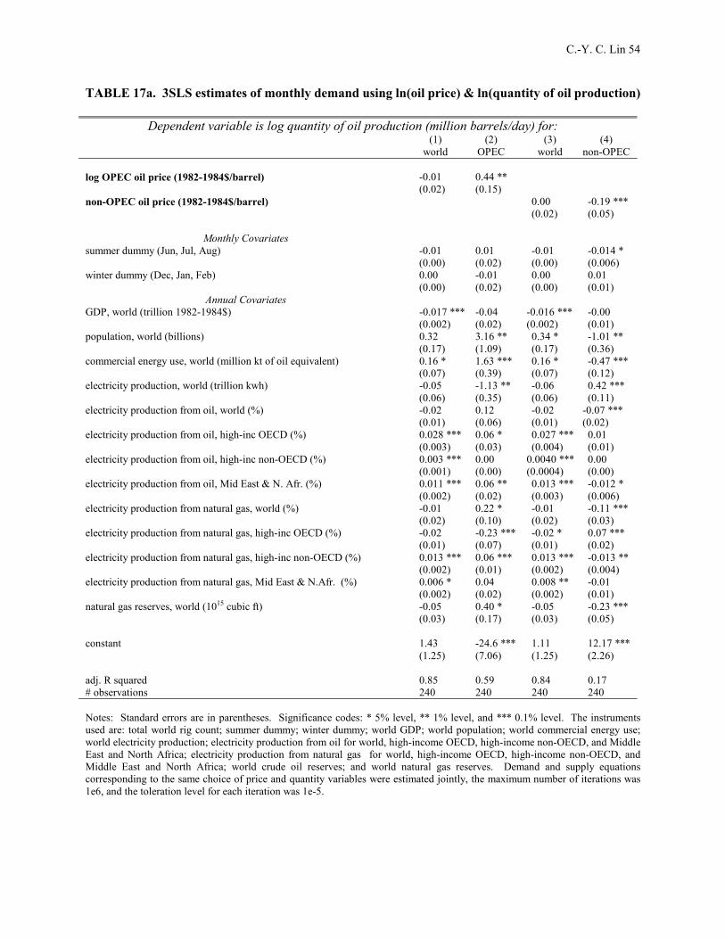
C.-Y. C. Lin 54

TABLE 17a. 3SLS estimates of monthly demand using ln(oil price) & ln(quantity of oil production)

Dependent variable is log quantity of oil production (million barrels/day) for: (1) (2) (3) (4) world OPEC world non-OPEC

log OPEC oil price (1982-1984$/barrel) -0.01

(0.02) 0.44 ** (0.15)

non-OPEC oil price (1982-1984$/barrel) 0.00 (0.02)

-0.19 *** (0.05)

Monthly Covariates

summer dummy (Jun, Jul, Aug) -0.01 (0.00)

0.01 (0.02)

-0.01 (0.00)

-0.014 * (0.006)

winter dummy (Dec, Jan, Feb) 0.00 (0.00)

-0.01 (0.02)

0.00 (0.00)

0.01 (0.01)

Annual Covariates GDP, world (trillion 1982-1984$) -0.017 ***

(0.002) -0.04 (0.02)

-0.016 *** (0.002)

-0.00 (0.01)

population, world (billions) 0.32 (0.17)

3.16 ** (1.09)

0.34 * (0.17)

-1.01 ** (0.36)

commercial energy use, world (million kt of oil equivalent) 0.16 * (0.07)

1.63 *** (0.39)

0.16 * (0.07)

-0.47 *** (0.12)

electricity production, world (trillion kwh) -0.05 (0.06)

-1.13 ** (0.35)

-0.06 (0.06)

0.42 *** (0.11)

electricity production from oil, world (%) -0.02 (0.01)

0.12 (0.06)

-0.02 (0.01)

-0.07 *** (0.02)

electricity production from oil, high-inc OECD (%) 0.028 *** (0.003)

0.06 * (0.03)

0.027 *** (0.004)

0.01 (0.01)

electricity production from oil, high-inc non-OECD (%) 0.003 *** (0.001)

0.00 (0.00)

0.0040 *** (0.0004)

0.00 (0.00)

electricity production from oil, Mid East & N. Afr. (%) 0.011 *** (0.002)

0.06 ** (0.02)

0.013 *** (0.003)

-0.012 * (0.006)

electricity production from natural gas, world (%) -0.01 (0.02)

0.22 * (0.10)

-0.01 (0.02)

-0.11 *** (0.03)

electricity production from natural gas, high-inc OECD (%) -0.02 (0.01)

-0.23 *** (0.07)

-0.02 * (0.01)

0.07 *** (0.02)

electricity production from natural gas, high-inc non-OECD (%) 0.013 *** (0.002)

0.06 *** (0.01)

0.013 *** (0.002)

-0.013 ** (0.004)

electricity production from natural gas, Mid East & N.Afr. (%) 0.006 * (0.002)

0.04 (0.02)

0.008 ** (0.002)

-0.01 (0.01)

natural gas reserves, world (1015 cubic ft) -0.05 (0.03)

0.40 * (0.17)

-0.05 (0.03)

-0.23 *** (0.05)

constant 1.43

(1.25) -24.6 *** (7.06)

1.11 (1.25)

12.17 *** (2.26)

adj. R squared 0.85 0.59 0.84 0.17 # observations 240 240 240 240 Notes: Standard errors are in parentheses. Significance codes: * 5% level, ** 1% level, and *** 0.1% level. The instruments used are: total world rig count; summer dummy; winter dummy; world GDP; world population; world commercial energy use; world electricity production; electricity production from oil for world, high-income OECD, high-income non-OECD, and Middle East and North Africa; electricity production from natural gas for world, high-income OECD, high-income non-OECD, and Middle East and North Africa; world crude oil reserves; and world natural gas reserves. Demand and supply equations corresponding to the same choice of price and quantity variables were estimated jointly, the maximum number of iterations was 1e6, and the toleration level for each iteration was 1e-5.

C.-Y. C. Lin 55

TABLE 17b. 3SLS estimates of monthly supply using ln(oil price) & ln(quantity of oil production)

Dependent variable is log quantity of oil production (million barrels/day) for: (1) (2) (3) (3) world OPEC world non-OPEC

log OPEC oil price (1982-1984$/barrel) -0.06 ***

(0.01) -0.12 *** (0.04)

non-OPEC oil price (1982-1984$/barrel) -0.05 *** (0.01)

-0.01 (0.01)

Monthly Covariates

total world rig count (100 rigs) 0.0008 * (0.0004)

0.008 *** (0.001)

0.00 (0.00)

-3.5e-3 *** (0.5e-3)

summer dummy (Jun, Jul, Aug) -0.01 (0.00)

-0.00 (0.01)

-0.01 (0.00)

-0.010 * (0.005)

winter dummy (Dec, Jan, Feb) 0.00 (0.00)

-0.02 (0.01)

0.00 (0.00)

0.012 * (0.005)

Annual Covariates GDP, Mid East & N.Afr. (trillion 1982-1984$) 0.78 ***

(0.06) 1.06 *** (0.17)

0.77 *** (0.06)

0.53 *** (0.06)

crude oil reserves, world (billion barrels) 4.6e-4 *** (0.2e-4)

0.0014 *** (0.0001)

4.8e-4 *** (0.2e-4)

-4.9e-5 * (2.2e-5)

constant 3.54 ***

(0.04) 1.65 *** (0.13)

3.51 *** (0.04)

3.57 *** (0.05)

adj. R squared 0.86 0.81 0.85 0.49 # observations 240 240 240 240 Notes: Standard errors are in parentheses. Significance codes: * 5% level, ** 1% level, and *** 0.1% level. The instruments used are: total world rig count; summer dummy; winter dummy; world GDP; world population; world commercial energy use; world electricity production; electricity production from oil for world, high-income OECD, high-income non-OECD, and Middle East and North Africa; electricity production from natural gas for world, high-income OECD, high-income non-OECD, and Middle East and North Africa; world crude oil reserves; and world natural gas reserves. Demand and supply equations corresponding to the same choice of price and quantity variables were estimated jointly, the maximum number of iterations was 1e6, and the toleration level for each iteration was 1e-5.

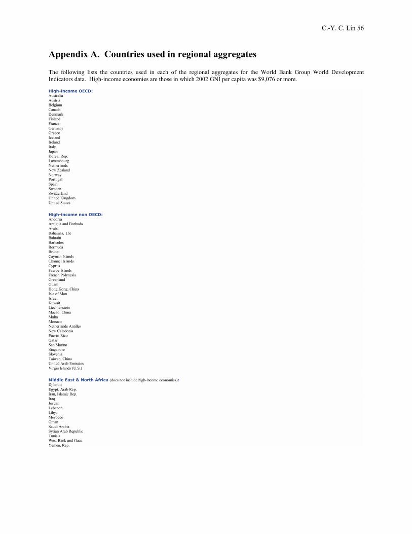
C.-Y. C. Lin 56

Appendix A. Countries used in regional aggregates The following lists the countries used in each of the regional aggregates for the World Bank Group World Development Indicators data. High-income economies are those in which 2002 GNI per capita was $9,076 or more. High-income OECD: Australia Austria Belgium Canada Denmark Finland France Germany Greece Iceland Ireland Italy Japan Korea, Rep. Luxembourg Netherlands New Zealand Norway Portugal Spain Sweden Switzerland United Kingdom United States High-income non OECD: Andorra Antigua and Barbuda Aruba Bahamas, The Bahrain Barbados Bermuda Brunei Cayman Islands Channel Islands Cyprus Faeroe Islands French Polynesia Greenland Guam Hong Kong, China Isle of Man Israel Kuwait Liechtenstein Macao, China Malta Monaco Netherlands Antilles New Caledonia Puerto Rico Qatar San Marino Singapore Slovenia Taiwan, China United Arab Emirates Virgin Islands (U.S.) Middle East & North Africa (does not include high-income economies): Djibouti Egypt, Arab Rep. Iran, Islamic Rep. Iraq Jordan Lebanon Libya Morocco Oman Saudi Arabia Syrian Arab Republic Tunisia West Bank and Gaza Yemen, Rep.