ESTABILIZATION TIME FOR SUBCRITICAL SYSTEM · PDF fileDriven System) type reactors ... section 4, we display the results and further discuss for the simulations. In section 5, we present

2013 International Nuclear Atlantic Conference - INAC 2013

Recife, PE, Brazil, November 24-29, 2013 ASSOCIAÇÃO BRASILEIRA DE ENERGIA NUCLEAR - ABEN

ISBN: 978-85-99141-05-2

ESTABILIZATION TIME FOR SUBCRITICAL SYSTEM WITH

DIFFERENT EXTERNAL NEUTRON SOURCE

Brayan S. Fonseca1, Fernando C. Silva

1 and Zelmo R. Lima

2

1 Programa de Engenharia Nuclear - COPPE

Universidade Federal do Rio de Janeiro

Av. Horácio Macedo, 2030

21941-972 Rio de Janeiro, RJ

[email protected]; [email protected]; [email protected]

2 Instituto de Engenharia Nuclear (IEN/CNEN – RJ)

Rua Hélio de Almeida,75

21941-906 Cidade Universitária RJ

[email protected]

ABSTRACT

This work aims at studying one dimensional spatial kinetics equations for ADS (Accelerator

Driven System) type reactors, through computational simulations. Where the neutrons

diffusion equations are discretized espatially by the finite differences cell centered mesh

scheme and time discretized using the Crank-Nicolson method. Discretized equations used

with fixed source problem are programmed in FORTRAN and used to simulate the system

behavior, with different neutron source types. In this way, we can analyse the instant of time

when the subcritical system becomes stationary, or the time interval corresponding to the

stationary flux, for different external sources. The result shows that, it is always possible to

reach system stability where no oscillation is detected, even for pulsed sources.

1. INTRODUCTION

The ADS (OECD, 2002) is an innovated system that uses a fast neutrons source through a

reaction entitled “spallation”. During spallation, neutrons are ejected from a heavy nucleus,

and then target a high energy particle; in the case accelerated protons that are derationed to a

material target in solid or liquid state (OECD, 2002).

The ADS reactor is a subcritical system that offers an intrinsic security in the potential of a

critical accident because the subcritical reactor estate avoids the fission chain reaction

without control; and so this system naturally turns off the reactor. In actual reactors, the

process turning off the device needs to be done through control bars. Thus, in accident cases,

this can not occurs and consequently, a without control fission chain reaction.

For the stability subcritical studying, we simulate through computer reenactment, a reactor

core Benchmark (NAGAYA, 1995) using the spatial kinetics equations (DUDARSTADT e

HAMILTON, 1976) discretized spatially by the finite differences cell centered mesh scheme

(Alvim, 2007) and time discretized using the Crank-Nicolson method (NAKAMURA, 1977).

mailto:[email protected]

mailto:[email protected]

INAC 2013, Recife, PE, Brazil.

In this way, we analysed the time interval corresponding to the stationary flux, for different

external sources.

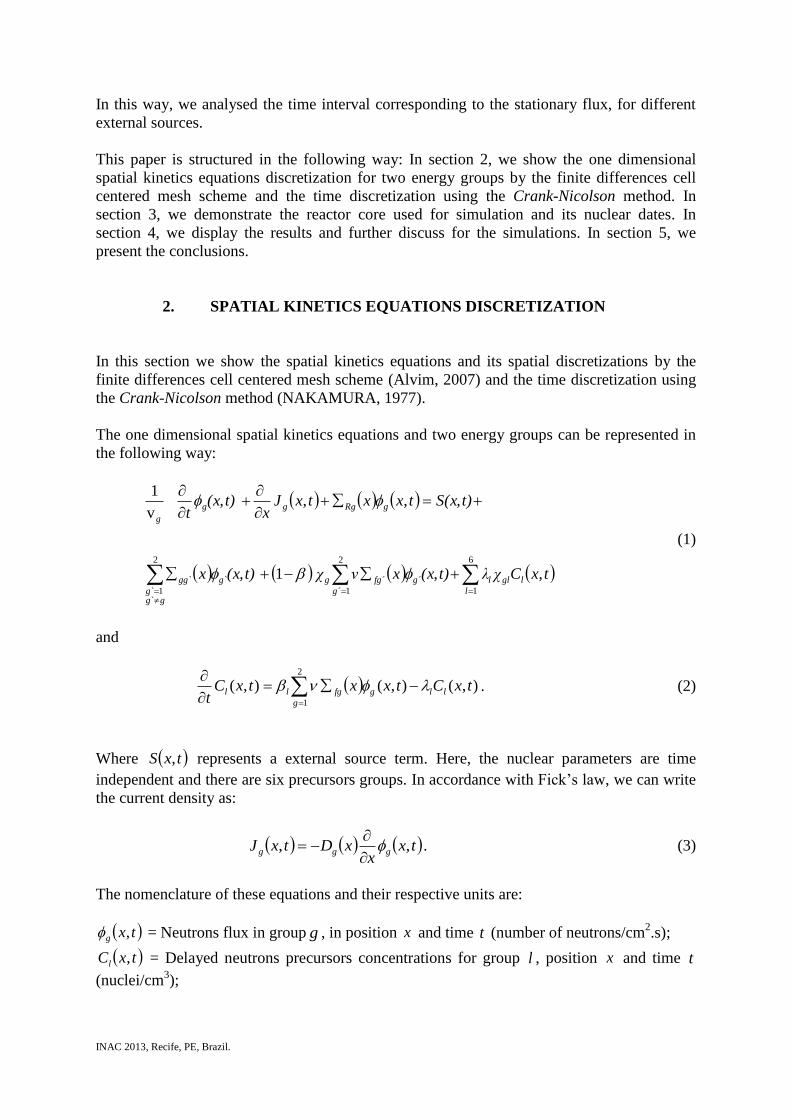
This paper is structured in the following way: In section 2, we show the one dimensional

spatial kinetics equations discretization for two energy groups by the finite differences cell

centered mesh scheme and the time discretization using the Crank-Nicolson method. In

section 3, we demonstrate the reactor core used for simulation and its nuclear dates. In

section 4, we display the results and further discuss for the simulations. In section 5, we

present the conclusions.

2. SPATIAL KINETICS EQUATIONS DISCRETIZATION

In this section we show the spatial kinetics equations and its spatial discretizations by the

finite differences cell centered mesh scheme (Alvim, 2007) and the time discretization using

the Crank-Nicolson method (NAKAMURA, 1977).

The one dimensional spatial kinetics equations and two energy groups can be represented in

the following way:

2

1

6

1

2

1

,,1,

,,,,v

1

g´ l

lgllg´fg´g

gg`g`

g`gg`

gRggg

g

txCχλt)(xxν χ t)(xx

t)S(xtxxtxJx

t) (x

t

(1)

and

2

1

),(),(),(g

llgfgll txCtxxtxCt

. (2)

Where txS , represents a external source term. Here, the nuclear parameters are time

independent and there are six precursors groups. In accordance with Fick’s law, we can write

the current density as:

txx

xDtxJ ggg ,,

. (3)

The nomenclature of these equations and their respective units are:

txg , = Neutrons flux in group g , in position x and time t (number of neutrons/cm2.s);

txCl , = Delayed neutrons precursors concentrations for group l , position x and time t

(nuclei/cm3);


l = Fraction of all fission neutrons emitted per fission that appears from l th precursor

group;

l = Decay constant of l th precursor group (s-1

);

gv = Neutron speed for group g (cm/s);

xDg Diffusion coefficient for group g in position x (cm);

xRg = Removal macroscopic cross section for group g in position x (cm-1

);

xgg` = Group-transfer macroscopic cross section from a group 'g to the group g in

position x (cm-1

);

xfg = Average number of neutrons released per fission multiplied by the fission

macroscopic cross sections in position x (cm-1

);

g = Neutrons fission spectrum for group g ;

gl = Delayed neutrons fission spectrum for energy group g and precursor group l .

2.1. Spatial Discretization

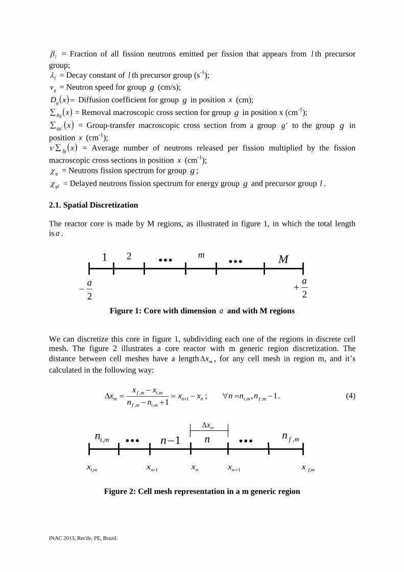
The reactor core is made by M regions, as illustrated in figure 1, in which the total length

is a .

Figure 1: Core with dimension a and with M regions

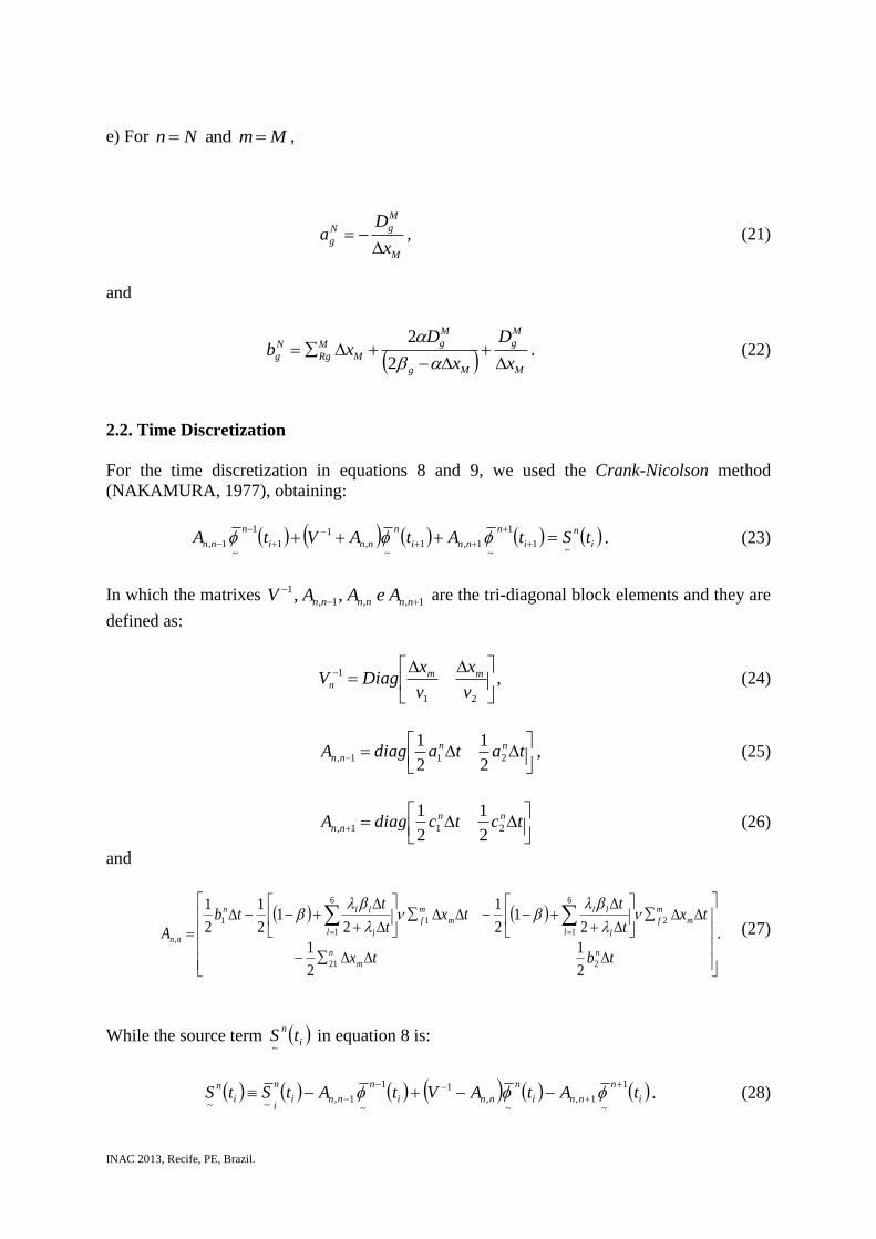
We can discretize this core in figure 1, subdividing each one of the regions in discrete cell

mesh. The figure 2 illustrates a core reactor with m generic region discretization. The

distance between cell meshes have a length mx , for any cell mesh in region m, and it’s

calculated in the following way:

1, ; 1

,,1

,,

,,

mfminn

mimf

mimf

m nnnxxnn

xxx . (4)

Figure 2: Cell mesh representation in a m generic region

f,mnnn-i,m x x x x x 11

min , 1n n mfn ,

mx

1 2 Mm

2

a

2

a


Now defining:

dxtxx

tn

n

x

x

g

m

n

g

1

,1

, (5)

dxtxCx

tCn

n

x

x

l

m

n

l

1

,1

(6)

and

dxtxSx

tSn

n

x

x

l

m

n

g

1

,1

. (7)

From equations 1, 2 e 3, we obtain:

6

1

2

'1'

'''

2

1'

11

g

1

v

l

n

lml

ggg

n

gm

m

gg

n

g

g

m

m

fgm

n

g

n

g

n

g

n

g

n

g

n

g

n

g

n

gm

tCxxtxxtS

tctbtatdt

dx

(8)

and

tCxtxtCdt

dx n

lml

g

n

gm

m

fgl

n

lm

2

1

. (9)

In which the constants n

g

n

g

n

g cba e , are so determined as:

a) For 1 and 1 mn ,

1

1

1

1

1

1

2

2

x

D

x

Dxb

g

g

g

Rg

n

g

(10)

and

1

1

1

x

Dc

g

g

. (11)


b) For 1 and , mnn mi ,

1

1

12

m

m

gm

m

g

m

g

m

gn

gxDxD

DDa , (12)

)( n

g

n

gm

m

Rg

n

g caxb (13)

and

m

m

gn

gx

Dc

. (14)

c) for Mmnn mf and , ,

m

m

gn

gx

Da

, (15)

)( n

g

n

gm

m

Rg

n

g caxb (16)

and

m

m

gm

m

g

m

g

m

gn

gxDxD

DDc

1

1

12. (17)

d) for mfmi nnn ,, and Mm1 ,

m

m

gn

gx

Da

, (18)

)( n

g

n

gm

m

Rg

n

g caxb (19)

and

m

m

gn

gx

Dc

. (20)


e) For MmNn and ,

M

M

gN

gx

Da

, (21)

and

M

M

g

Mg

M

g

M

M

Rg

N

gx

D

x

Dxb

2

2. (22)

2.2. Time Discretization

For the time discretization in equations 8 and 9, we used the Crank-Nicolson method

(NAKAMURA, 1977), obtaining:

i

n

i

n

nni

n

nni

n

nn tStAtAVtA~

1

1

~1,1

~,

1

1

1

~1,

. (23)

In which the matrixes 1,,1,

1 , ,

nnnnnn AeAAV are the tri-diagonal block elements and they are

defined as:

21

1

v

x

v

xDiagV mm

n , (24)

tatadiagA nn

nn 211,2

1

2

1, (25)

tctcdiagA nn

nn 211,2

1

2

1 (26)

and

.

2

1

2

1

21

2

1

21

2

1

2

1

221

2

6

1

1

6

1

1

,

tbtx

txt

ttx

t

ttb

An

m

n

m

m

f

l l

ll

m

m

f

l l

lln

nn

(27)

While the source term i

ntS

~ in equation 8 is:

in

nni

n

nni

n

nni

n

ii

ntAtAVtAtStS

1

~1,

~,

11

~1,

~~

. (28)


In which:

tS

tCt

xttS

Sn

i

l

i

n

l

l

mln

in

i

,2

6

1

,1

~2

2

. (29)

So, to solve the equation (23), in each step of time 1it , we use the called Thomas Algorithms

(Alvim, 2007), besides a known spatial and time neutron source.

3. BENCHMARK ANL BSS-6-A2 PRESENTATION

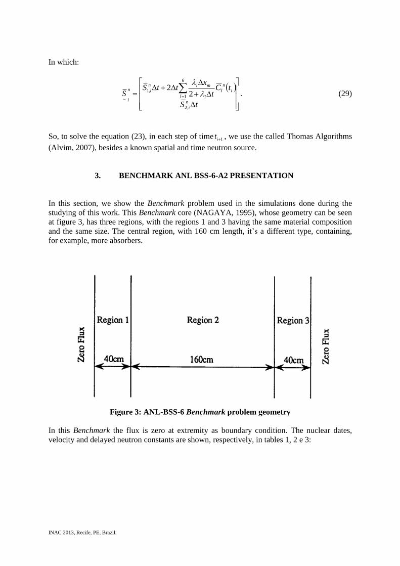
In this section, we show the Benchmark problem used in the simulations done during the

studying of this work. This Benchmark core (NAGAYA, 1995), whose geometry can be seen

at figure 3, has three regions, with the regions 1 and 3 having the same material composition

and the same size. The central region, with 160 cm length, it’s a different type, containing,

for example, more absorbers.

Figure 3: ANL-BSS-6 Benchmark problem geometry

In this Benchmark the flux is zero at extremity as boundary condition. The nuclear dates,

velocity and delayed neutron constants are shown, respectively, in tables 1, 2 e 3:


Table 1: ANL-BSS-6 Benchmark problem nuclear parameters

Constant Region 1 e 3 Region 2

)(1 cmD 1.5 1.0

)(2 cmD 0.5 0.5

)( 1

1

cmR 0.026 0.02

)( 1

2

cmR 0.18 0.08

)( 1

12

cms 0.015 0.01

)( 1

1

cmf

0.01 0.005

)( 1

2

cmf

0.2 0.099

Table 2: ANL-BSS-6 Benchmark problem neutron velocity

g )/( scmvg 1 7100.1

2 5100.3

Table 3: ANL-BSS-6 Benchmark problem delayed neutron constants

l l )( 1sl

1 0.00025 0.0124

2 0.00164 0.0305

3 0.00147 0.1110

4 0.00296 0.3010

5 0.00086 1.1400

6 0.00032 3.0100

In order to obtain different subcritical systems, from Benchmark, removing macroscopic

cross section values were altered, through maintaining invariable the others nuclear

parameters. The table 4 shows the removing macroscopic cross section values in each region,

for the two energy groups, and the multiplication factor associated.

Table 4: Removing macroscopic cross section ( m

Rg ) and the multiplication factor ( effk )

associated

11

1

cmR 11

2

cmR 12

1

cmR 12

2

cmR effk

0.025 0.176 0.019 0.079 0.951142

0.0245 0.176 0.019 0.079 0.962169

0.0245 0.176 0.0185 0.079 0.971960

0.0245 0.176 0.0185 0.077 0.980073

0.0239 0.176 0.0185 0.077 0.991892


4. RESULTS ANALYZED

We show, in this section, the results obtained with the computational simulation. For all the

cases, the distance between each cell mesh ( mx ) was 1 cm, in any region. This totalizes 240

cell meshes.

The neutron external source was adjusted to have a neutron flux in order 1015

nêutrons/cm2.s,

existing for the fast energy group and being zero for the termical group, because we are

simulating subcritical systems like ADS reactor type. In all cases considered, the time

interval between steps of time were s510 , with flux always equal to zero at initial instant.

The results shown are as follows; the flux stabilization time , for the different subcritical

systems and external neutron source. Some different cases were considered for this finality: i)

punctual source localized in 0x , emitting scmneutrons ./10 214 ; ii) Source centered in

reactor core, occupying 10 cm length, emitting scmneutrons ./10 313 ; iii) distributed source

through the entire reactor core, emitting scmneutrons ./10 312 .

In the next subsections are shown, separately, the results for the cases with external source

with constant and varying time intensity, respectively.

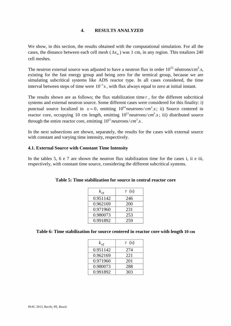
4.1. External Source with Constant Time Intensity

In the tables 5, 6 e 7 are shown the neutron flux stabilization time for the cases i, ii e iii,

respectively, with constant time source, considering the different subcritical systems.

Table 5: Time stabilization for source in central reactor core

effk (s)

0.951142 246

0.962169 200

0.971960 231

0.980073 253

0.991892 259

Table 6: Time stabilization for source centered in reactor core with length 10 cm

effk

(s)

0.951142 274

0.962169 221

0.971960 201

0.980073 288

0.991892 303


Table 7: Time stabilization for source distributed through the entire reactor core

effk

(s)

0.951142 205

0.962169 217

0.971960 253

0.980073 255

0.991892 255

4.2. External Source with Varying Time Intensity

For this case, the time shape, adopted for the source, is descripted below:

oo S

T

tt

1 . (30)

In which 0S is the intensity of the source, in accordance with the cases i, ii e iii and T is the

period in seconds. The graphic representation of this source, for a period T equal to 0,01s and

oS from case i, is shown in figure 4.

0,0 0,5 1,0 1,5 2,0

0,00E+000

2,00E+009

4,00E+009

6,00E+009

8,00E+009

1,00E+010

Inte

nsid

ade

(nêu

tron

s/cm

3.s

)

Tempo (s)

T=0,5 s

Figure 4 – Source intensity in time function

The neutron flux stabilization time, considering the different subcritical systems, for oS from

the cases i, ii and iii, respectively, they are shown in tables 8, 9 e 10.


Table 8: Time stabilization for source in central reactor core

(s)

effk

T=0,01s T=0,001s

0.951142 195 214

0.962169 224 247

0.971960 197 230

0.980073 272 269

0.991892 274 309

Table 9: Time stabilization for source centered in reactor core with length 10 cm

(s)

effk

T=0,01s T=0,001s

0.951142 200 208

0.962169 191 285

0.971960 265 222

0.980073 194 258

0.991892 261 271

Table 10: Time stabilization for source distributed through the entire reactor core

(s)

effk

T=0,01s T=0,001s

0.951142 287 201

0.962169 216 255

0.971960 197 198

0.980073 271 202

0.991892 237 228

We can see, with the results shown in tables 8, 9 and 10, that, the flux time stabilization

doesn’t vary so much between the positions and intensity of the varying time external source.

Although, for the cases with constant time external sources, we see that the flux stabilization

time tends to increase at the criticality proximity.


5. CONCLUSIONS

In accordance with the results obtained by the spatial kinetics program (1-D/2-G), we

conclude that constant time external sources, in all the cases examined, the flux stabilization

time increases with multiplication factor effk , or the stabilization increases at the criticality

proximities.

For the varying time external source we see that the system reached the stabilization for all

the periods or frequency of neutron pulsed emitting and for different position or intensity of

the neutron source. None oscillation was detected in these results, even with pulsed source.

We can conclude also, that according to the methodology work, we were able to obtain,

neutron flux stabilization time for subcritical systems with different external neutron sources.

In spite of future studying perspectives, we can extend this numerical computing to more than

one dimension; use others external neutron sources types or shapes, use algorithms and

different discretization techniques for the process of neutrons diffusion equations.

REFERENCES

1. A.C. M. Alvim, Métodos Numéricos em Engenharia Nuclear, Ed. Certa, Curitiba-Brasil

(2007).

2. J.J. Dudestadt and L.J. Hamilton, Nuclear Reactor Analysis, New York-USA, John Wiley

& Sons (1976).

3. F. Inanc, “A Coarse Mesh Nodal Method For One-Dimensional Spatial Kinetics

Calculations”, Ann. NucL Energy, V. 24, No. 4, pp. 257-265 (1997).

4. Y. Nagaya and K. Kobayashi, “Solution of 1-D Mult-Group Time-Dependent Diffusion

Equations Using The Coupled Reactor Theory”, Ann. NucL Energy, V.22, N.7, pp.421-

140 (1995).

5. S. Nakamura, Computational Method in Engineering and Science, John Wiley & Sons,

New York-USA (1977).

6. “OECD-Accelerator-driven Systems (ADS) and Fast Reactors (FR) in Advanced Nuclear

Fuel Cycles”, https://www.oecd-nea.org/ndd/reports/2002/nea3109-ads.pdf (2002).

7. T. M. Sutton and B. N. Aviles, “Diffusion Theory Method For Spatial Kinetics

Calculations”, Progress in Nuclear Energy, V.30, N.2, pp.119-182 (1996).

8. R. L. Zelmo, “Aplicação do Método dos Pseudo-Harmônicos à Cinética

Multidimensional”, Tese de D.Sc., COPPE/UFRJ, Rio de Janeiro-Brasil (2005).

9. “The Generation IV International Forum (GIF)”, http://www.gen-4.org/index.html

(2012).

https://www.oecd-nea.org/ndd/reports/2002/nea3109-ads.pdf

http://www.gen-4.org/index.html

Documents

ESTABILIZATION TIME FOR SUBCRITICAL SYSTEM · PDF fileDriven System) type reactors ... section 4, we display the results and further discuss for the simulations. In section 5, we present