Embed Size (px)
Citation preview


Essential MATLABfor Engineers and Scientists
Fourth Edition
Brian H. Hahn
Daniel T. Valentine
AMSTERDAM • BOSTON • HEIDELBERG • LONDONNEW YORK • OXFORD • PARIS • SAN DIEGO
SAN FRANCISCO • SINGAPORE • SYDNEY • TOKYOAcademic Press is an imprint of Elsevier

Academic Press is an imprint of Elsevier30 Corporate Drive, Suite 400, Burlington, MA 01803, USALinacre House, Jordan Hill, Oxford OX2 8DP, UK
Copyright © 2010, Daniel T. Valentine. Published by Elsevier Ltd. All rights reserved.
MATLAB® is a trademark of The MathWorks, Inc. and is used with permission.The MathWorks does not warrant the accuracy of the text or exercises in this book.This book’s use or discussion of MATLAB® software or related products does notconstitute endorsement or sponsorship by The MathWorks of a particular pedagogicalapproach or particular use of the MATLAB® software.
No part of this publication may be reproduced, stored in a retrieval system, ortransmitted in any form or by any means, electronic, mechanical, photocopying,recording, or otherwise, without the prior written permission of the publisher.
Permissions may be sought directly from Elsevier’s Science & Technology RightsDepartment in Oxford, UK: phone: (+44) 1865 843830, fax: (+44) 1865 853333,E-mail: [email protected]. You may also complete your request online viathe Elsevier homepage (http://www.elsevier.com), by selecting “Support & Contact”then “Copyright and Permission” and then “Obtaining Permissions.”
Library of Congress Cataloging-in-Publication DataA catalog record for this book is available from the Library of Congress.
British Library Cataloguing-in-Publication DataA catalogue record for this book is available from the British Library.
ISBN: 978-0-12-374883-6
For information on all Academic Press publicationsvisit our Web site at www.elsevierdirect.com
Typeset by: diacriTech, India
Printed in Canada09 10 11 12 13 10 9 8 7 6 5 4 3 2 1

Preface
The main reason for a fourth edition of Essential MATLAB for Engineers andScientists is to keep up with MATLAB, now in its latest version (7.7 Version2008B). Like the previous editions, this one presents MATLAB as a problem-solving tool for professionals in science and engineering, as well as students inthose fields, who have no prior knowledge of computer programming.
In keeping with the late Brian D. Hahn’s objectives in previous editions,the fourth edition adopts an informal, tutorial style for its “teach-yourself”approach, which invites readers to experiment with MATLAB as a way of dis-covering how it works. It assumes that readers have never used this tool in theirtechnical problem solving.
MATLAB, which stands for “Matrix Laboratory,” is based on the concept ofthe matrix. Because readers will be unfamiliar with matrices, ideas and con-structs are developed gradually, as the context requires. The primary audiencefor Essential MATLAB is scientists and engineers, and for that reason certainexamples require some first-year college math, particularly in Part 2. However,these examples are self-contained and can be skipped without detracting fromthe development of readers’ programming skills.
MATLAB can be used in two distinct modes. One, in keeping the modern-age craving for instant gratification, offers immediate execution of statements(or groups of statements) in the Command Window. The other, for the morepatient, offers conventional programming by means of script files. Both modesare put to good use here: the former encouraging cut and paste to take full advan-tage of Windows’ interactive environment; the latter stressing programmingprinciples and algorithm development through structure plans.
Although most of MATLAB’s basic (“essential”) features are covered, this book isneither an exhaustive nor a systematic reference. This would not be in keepingwith its informal style. For example, constructs such as for and if are notalways treated, initially, in their general form, as is common in many texts,but are gradually introduced in discussions where they fit naturally. Even so,they are treated thoroughly here, unlike in other texts that deal with them only xvii

xviii Preface
superficially. For the curious, helpful syntax and function quick references canbe found in the appendices.
The following list contains other highlights of Essential MATLAB for Engineersand Scientists, Fourth Edition:
■ Warnings of the many pitfalls that await the unwary beginner
■ Numerous examples taken from science and engineering (simulation,population modeling, numerical methods) as well as business andeveryday life
■ An emphasis on programming style to produce clear, readable code
■ Comprehensive chapter summaries
■ Chapter exercises (answers and solutions to many of which are given inan appendix)
■ A thorough, instructive index
Essential MATLAB is meant to be used in conjunction with the MATLAB software.The reader is expected to have the software at hand in order to work throughthe exercises and thus discover how MATLAB does what it is commandedto do. Learning any tool is possible only through hands-on experience. Thisis particularly true with computing tools, which produce correct answers onlywhen the commands they are given and the accompanying data input arecorrect and accurate.
ACKNOWLEDGMENTS
I would like to thank Mary, Clara, and Zach for their support, and I dedicatethe fourth edition of Essential MATLAB for Engineers and Scientists to them.
Daniel T. Valentine

Contents
PREFACE...................................................................................... xvii
Part 1 Essentials 1
CHAPTER 1 Introduction ........................................................... 3
1.1 Using MATLAB ................................................... 5
1.1.1 Arithmetic................................................. 5
1.1.2 Variables................................................... 7
1.1.3 Mathematical functions .............................. 8
1.1.4 Functions and commands ........................... 9
1.1.5 Vectors ..................................................... 9
1.1.6 Linear equations ........................................ 11
1.1.7 Demo........................................................ 12
1.1.8 Help ......................................................... 12
1.1.9 Additional features .................................... 131.2 The MATLAB Desktop.......................................... 151.3 Sample Program .................................................. 16
1.3.1 Cut and paste ............................................ 16
1.3.2 Saving a program: script files ...................... 18
1.3.3 A program in action.................................... 19Summary ................................................................... 21Chapter Exercises ....................................................... 21
CHAPTER 2 MATLAB Fundamentals .......................................... 23
2.1 Variables ............................................................ 23
2.1.1 Case sensitivity ......................................... 242.2 The Workspace.................................................... 24
2.2.1 Adding commonly used constants to theworkspace ................................................ 25
v

vi Contents
2.3 Arrays: Vectors and Matrices ................................ 26
2.3.1 Initializing vectors: Explicit lists .................. 26
2.3.2 Initializing vectors: The colon operator ......... 27
2.3.3 The linspace function............................... 28
2.3.4 Transposing vectors ................................... 28
2.3.5 Subscripts ................................................. 28
2.3.6 Matrices ................................................... 29
2.3.7 Capturing output ....................................... 302.4 Vertical Motion Under Gravity ............................... 302.5 Operators, Expressions, and Statements ................. 32
2.5.1 Numbers................................................... 33
2.5.2 Data types................................................. 34
2.5.3 Arithmetic operators .................................. 34
2.5.4 Operator precedence .................................. 34
2.5.5 The colon operator ..................................... 35
2.5.6 The transpose operator............................... 36
2.5.7 Arithmetic operations on arrays................... 36
2.5.8 Expressions............................................... 37
2.5.9 Statements................................................ 38
2.5.10 Statements, commands, and functions.......... 39
2.5.11 Formula vectorization ................................. 392.6 Output................................................................ 42
2.6.1 The disp statement ................................... 42
2.6.2 The format command ................................ 43
2.6.3 Scale factors .............................................. 452.7 Repeating with for.............................................. 45
2.7.1 Square roots with Newton’s method............. 46
2.7.2 Factorials! ................................................. 47
2.7.3 Limit of a sequence .................................... 47
2.7.4 The basic for construct.............................. 48
2.7.5 for in a single line ..................................... 50
2.7.6 More general for ....................................... 50
2.7.7 Avoid for loops by vectorizing! ................... 502.8 Decisions ............................................................ 53
2.8.1 The one-line if statement .......................... 53
2.8.2 The if-else construct............................... 55
2.8.3 The one-line if-else statement ................. 56
2.8.4 elseif ..................................................... 56
2.8.5 Logical operators ....................................... 57

Contents vii
2.8.6 Multiple ifs versus elseif ........................ 58
2.8.7 Nested ifs................................................ 59
2.8.8 Vectorizing ifs? ........................................ 60
2.8.9 The switch statement ............................... 602.9 Complex Numbers ............................................... 612.10 More on Input and Output .................................... 63
2.10.1 fprintf ................................................... 63
2.10.2 Output to a disk file with fprintf ............... 64
2.10.3 General file I/O .......................................... 65
2.10.4 Saving and loading data.............................. 652.11 Odds and Ends .................................................... 65
2.11.1 Variables, functions, and scripts with thesame name................................................ 65
2.11.2 The input statement ................................. 66
2.11.3 Shelling out to the operating system ............ 67
2.11.4 More Help functions ................................... 672.12 Programming Style............................................... 67Summary ................................................................... 68Chapter Exercises ....................................................... 71
CHAPTER 3 Program Design and Algorithm Development .......... 77
3.1 The Program Design Process ................................. 78
3.1.1 The projectile problem................................ 803.2 Structure Plan Examples ....................................... 85
3.2.1 Quadratic equation .................................... 863.3 Structured Programming with Functions................. 88Summary ................................................................... 88Chapter Exercises ....................................................... 88
CHAPTER 4 MATLAB Functions and Data Import–ExportUtilities.................................................................... 91
4.1 Common Functions .............................................. 914.2 Importing and Exporting Data ............................... 96
4.2.1 The load and save commands .................... 96
4.2.2 Exporting text (ASCII) data ......................... 97
4.2.3 Importing text (ASCII) data ......................... 97
4.2.4 Exporting and importing binary data............ 97
4.2.5 The Import Wizard ..................................... 98
4.2.6 *Low-level file I/O functions ........................ 98
4.2.7 *Other import/export functions .................... 103

viii Contents
Summary ................................................................... 103Chapter Exercises ....................................................... 104
CHAPTER 5 Logical Vectors ........................................................ 107
5.1 Examples ............................................................ 108
5.1.1 Discontinuous graphs ................................. 108
5.1.2 Avoiding division by zero ............................ 109
5.1.3 Avoiding infinity ........................................ 110
5.1.4 Counting random numbers.......................... 111
5.1.5 Rolling dice ............................................... 1125.2 Logical Operators ................................................ 113
5.2.1 Operator precedence .................................. 114
5.2.2 Incorrect conversion ................................... 115
5.2.3 Logical operators and vectors ...................... 1155.3 Subscripting with Logical Vectors .......................... 1165.4 Logical Functions................................................. 117
5.4.1 Using any and all ..................................... 1185.5 Logical Vectors Instead of elseif Ladders ............. 119Summary ................................................................... 122Chapter Exercises ....................................................... 122
CHAPTER 6 Matrices of Numbers and Arrays of Strings ............. 125
6.1 Matrices ............................................................. 126
6.1.1 A concrete example.................................... 126
6.1.2 Creating matrices ...................................... 127
6.1.3 Subscripts ................................................. 127
6.1.4 The transpose operator............................... 128
6.1.5 The colon operator ..................................... 128
6.1.6 Duplicating rows and columns: Tiling .......... 132
6.1.7 Deleting rows and columns ......................... 132
6.1.8 Elementary matrices .................................. 133
6.1.9 Specialized matrices ................................... 134
6.1.10 Using MATLAB functions with matrices ....... 135
6.1.11 Manipulating matrices................................ 136
6.1.12 Array (element-by-element) operationson matrices ............................................... 136
6.1.13 Matrices and for ....................................... 137
6.1.14 Visualization of matrices ............................. 137

Contents ix
6.1.15 Vectorizing nested fors: Loan repaymenttables ....................................................... 137
6.1.16 Multidimensional arrays ............................. 1406.2 Matrix Operations ................................................ 140
6.2.1 Multiplication ............................................ 140
6.2.2 Exponentiation .......................................... 1426.3 Other Matrix Functions......................................... 1436.4 *Strings .............................................................. 143
6.4.1 Input ........................................................ 143
6.4.2 Strings as arrays ........................................ 144
6.4.3 String concatenation .................................. 144
6.4.4 ASCII codes: double and char.................... 144
6.4.5 String display with fprintf ....................... 146
6.4.6 Comparing strings ..................................... 146
6.4.7 Other string functions ................................ 1466.5 *Two-Dimensional Strings..................................... 1476.6 *eval and Text Macros......................................... 148
6.6.1 Error trapping with eval and lasterr......... 148
6.6.2 eval with try...catch............................. 149Summary ................................................................... 150Chapter Exercises ....................................................... 150
CHAPTER 7 Introduction to Graphics .......................................... 153
7.1 Basic Two-Dimensional Graphs ............................. 153
7.1.1 Labels ...................................................... 155
7.1.2 Multiple plots on the same axes................... 155
7.1.3 Line styles, markers, and color..................... 156
7.1.4 Axis limits................................................. 156
7.1.5 Multiple plots in a figure: subplot .............. 157
7.1.6 figure, clf, and cla................................. 159
7.1.7 Graphical input.......................................... 159
7.1.8 Logarithmic plots ....................................... 159
7.1.9 Polar plots ................................................. 160
7.1.10 Plotting rapidly changing mathematicalfunctions: fplot........................................ 161
7.1.11 The Property Editor .................................... 1627.2 Three-Dimensional Plots ....................................... 162
7.2.1 The plot3 function .................................... 162
7.2.2 Animated 3D plots with thecomet3 function ........................................ 163

x Contents
7.2.3 Mesh surfaces ........................................... 163
7.2.4 Contour plots............................................. 165
7.2.5 Cropping a surface with NaNs...................... 167
7.2.6 Visualizing vector fields .............................. 167
7.2.7 Matrix visualization.................................... 168
7.2.8 3D graph rotation ....................................... 169
7.2.9 Other graphics functions............................. 170Summary ................................................................... 178Chapter Exercises ....................................................... 179
CHAPTER 8 Loops ....................................................................... 185
8.1 Determinate Repetition with for ........................... 185
8.1.1 Binomial coefficient .................................... 185
8.1.2 Update processes....................................... 186
8.1.3 Nested fors .............................................. 1888.2 Indeterminate Repetition with while ..................... 188
8.2.1 A guessing game ....................................... 188
8.2.2 The while statement ................................. 189
8.2.3 Doubling time of an investment ................... 190
8.2.4 Prime numbers .......................................... 191
8.2.5 Projectile trajectory .................................... 192
8.2.6 break ....................................................... 194
8.2.7 Menus ...................................................... 195Summary ................................................................... 196Chapter Exercises ....................................................... 197
CHAPTER 9 Errors and Pitfalls .................................................... 201
9.1 Syntax Errors ...................................................... 201
9.1.1 Incompatible vector sizes............................ 202
9.1.2 Name hiding ............................................. 2029.2 Logic Errors ........................................................ 2029.3 Rounding Error .................................................... 203Summary ................................................................... 204Chapter Exercises ....................................................... 204
CHAPTER 10 Function M-files ....................................................... 207
10.1 Inline Objects: Harmonic Oscillators ...................... 20710.2 Function M-files: Newton’s Method Revisited ......... 20910.3 Basic Rules ......................................................... 210
10.3.1 Subfunctions ............................................. 215

Contents xi
10.3.2 Private functions........................................ 215
10.3.3 P-code files................................................ 215
10.3.4 Improving M-file performance with theprofiler...................................................... 215
10.4 Function Handles................................................. 21610.5 Command/Function Duality................................... 21710.6 Function Name Resolution .................................... 21810.7 Debugging M-files ............................................... 219
10.7.1 Debugging a script..................................... 219
10.7.2 Debugging a function ................................. 22110.8 Recursion............................................................ 221Summary ................................................................... 222Chapter Exercises ....................................................... 224
CHAPTER 11 Vectors as Arrays and *Advanced DataStructures ................................................................ 227
11.1 Update Processes................................................. 227
11.1.1 Unit time steps .......................................... 228
11.1.2 Non–unit time steps ................................... 230
11.1.3 Using a function......................................... 231
11.1.4 Exact solution............................................ 23311.2 Frequencies, Bar Charts, and Histograms ............... 233
11.2.1 A random walk .......................................... 233
11.2.2 Histograms ............................................... 23511.3 *Sorting .............................................................. 235
11.3.1 Bubble sort ............................................... 236
11.3.2 MATLAB’s sort ........................................ 23711.4 *Structures.......................................................... 23811.5 *Cell Arrays ........................................................ 240
11.5.1 Assigning data to cell arrays ....................... 240
11.5.2 Accessing data in cell arrays ....................... 242
11.5.3 Using cell arrays ........................................ 242
11.5.4 Displaying and visualizing cell arrays ........... 24311.6 *Classes and Objects............................................ 244Summary ................................................................... 244
CHAPTER 12 *More Graphics ........................................................ 245
12.1 Handle Graphics .................................................. 245
12.1.1 Getting handles ......................................... 246
12.1.2 Changing graphics object properties ............ 247

xii Contents
12.1.3 A vector of handles .................................... 248
12.1.4 Graphics object creation functions ............... 249
12.1.5 Parenting .................................................. 249
12.1.6 Positioning figures ..................................... 25012.2 Editing Plots ....................................................... 251
12.2.1 Plot edit mode ........................................... 251
12.2.2 Property Editor .......................................... 25212.3 Animation........................................................... 253
12.3.1 Animation with Handle Graphics ................. 25412.4 Colormaps .......................................................... 256
12.4.1 Surface plot color ....................................... 258
12.4.2 Truecolor .................................................. 25912.5 Lighting and Camera............................................ 25912.6 Saving, Printing, and Exporting Graphs .................. 260
12.6.1 Saving and opening figure files .................... 260
12.6.2 Printing a graph......................................... 260
12.6.3 Exporting a graph ...................................... 261Summary ................................................................... 261Chapter Exercises ....................................................... 262
CHAPTER 13 *Graphical User Interfaces (GUIs) ............................ 263
13.1 Basic Structure of a GUI ........................................ 26313.2 A First Example: Getting the Time......................... 26413.3 Newton’s Method Yet Again.................................. 26813.4 Axes on a GUI ..................................................... 27113.5 Adding Color to a Button ...................................... 272Summary ................................................................... 273
Part 2 Applications 275
CHAPTER 14 Dynamical Systems .................................................. 277
14.1 Cantilever Beam .................................................. 27814.2 Electric Current ................................................... 27914.3 Free Fall ............................................................. 28114.4 Projectile with Friction ......................................... 291Summary ................................................................... 294Chapter Exercises ....................................................... 295
CHAPTER 15 Simulation ................................................................ 297
15.1 Random Number Generation ................................. 297
15.1.1 Seeding rand ............................................ 298

Contents xiii
15.2 Flipping Coins ..................................................... 29815.3 Rolling Dice......................................................... 29915.4 Bacterium Division ............................................... 30015.5 A Random Walk ................................................... 30015.6 Traffic Flow......................................................... 30215.7 Normal (Gaussian) Random Numbers ..................... 305Summary ................................................................... 305Chapter Exercises ....................................................... 306
CHAPTER 16 *More Matrices ........................................................ 309
16.1 Leslie Matrices: Population Growth ....................... 30916.2 Markov Processes ................................................ 313
16.2.1 A random walk .......................................... 31316.3 Linear Equations ................................................. 315
16.3.1 MATLAB’s solution .................................... 316
16.3.2 The residual .............................................. 317
16.3.3 Overdetermined systems ............................ 317
16.3.4 Underdetermined systems .......................... 318
16.3.5 Ill-conditioned systems ............................... 318
16.3.6 Matrix division .......................................... 31916.4 Sparse Matrices ................................................... 320Summary ................................................................... 323Chapter Exercises ....................................................... 323
CHAPTER 17 *Introduction to Numerical Methods ........................ 325
17.1 Equations ........................................................... 325
17.1.1 Newton’s method....................................... 325
17.1.2 The Bisection method................................. 328
17.1.3 The fzero and roots functions .................. 32917.2 Integration .......................................................... 330
17.2.1 The Trapezoidal rule .................................. 330
17.2.2 Simpson’s rule ........................................... 331
17.2.3 The quad function...................................... 33217.3 Numerical Differentiation...................................... 332
17.3.1 The diff function...................................... 33317.4 First-Order Differential Equations .......................... 334
17.4.1 Euler’s method .......................................... 334
17.4.2 Example: Bacteria colony growth................. 335
17.4.3 Alternative subscript notation ..................... 336
17.4.4 A predictor-corrector method....................... 338

xiv Contents
17.5 Linear Ordinary Differential Equations ................... 33917.6 Runge-Kutta Methods .......................................... 339
17.6.1 A single differential equation ...................... 339
17.6.2 Systems of differential equations: Chaos ...... 340
17.6.3 Passing additional parameters to an ODEsolver ....................................................... 343
17.7 A Partial Differential Equation ............................... 344
17.7.1 Heat conduction ........................................ 34417.8 Other Numerical Methods ..................................... 348Summary ................................................................... 349Chapter Exercises ....................................................... 349
CHAPTER 18 Toolboxes That Come with MATLAB(online chapter: www.elsevierdirect.com/companions/978012374883-6)
APPENDIX A Syntax: Quick Reference ......................................... 353
A.1 Expressions ........................................................ 353A.2 Function M-files................................................... 353A.3 Graphics ............................................................. 353A.4 if and switch .................................................... 354A.5 for and while .................................................... 355A.6 Input/output........................................................ 356A.7 load/save .......................................................... 356A.8 Vectors and Matrices............................................ 357
APPENDIX B Operators ................................................................ 359
APPENDIX C Command and Function: Quick Reference .............. 361
C.1 General-Purpose Commands ................................. 361
C.1.1 Managing variables and the workspace ........ 361
C.1.2 Files and the operating system .................... 361
C.1.3 Controlling the Command Window .............. 362
C.1.4 Starting and quitting MATLAB .................... 362C.2 Logical Functions................................................. 362C.3 MATLAB Programming Tools ................................ 362
C.3.1 Interactive input ........................................ 363C.4 Matrices ............................................................. 363
C.4.1 Special variables and constants ................... 363
C.4.2 Time and date ........................................... 363
C.4.3 Matrix manipulation ................................... 363
C.4.4 Specialized matrices ................................... 364

Contents xv
C.5 Mathematical Functions ....................................... 364C.6 Matrix Functions ................................................. 365C.7 Data Analysis ...................................................... 365C.8 Polynomial Functions ........................................... 365C.9 Function Functions .............................................. 366C.10 Sparse Matrix Functions ....................................... 366C.11 Character String Functions.................................... 366C.12 File I/O Functions ................................................ 366C.13 2D Graphics ........................................................ 366C.14 3D Graphics ........................................................ 367C.15 General .............................................................. 367
APPENDIX D ASCII Character Codes ............................................ 369
APPENDIX E Solutions to Selected Exercises ............................... 371
INDEX .......................................................................................... 383

1PART
Essentials
Part 1 concerns those aspects of MATLAB that you need to know in order tocome to grips with MATLAB’s essentials and those of technical computing.Chapters 11, 12, and 13 are marked with an asterisk, as are certain sections inother chapters. These sections and chapters can be skipped in your first readingand line-by-line execution of the MATLAB commands and scripts described.Because this book is a tutorial, you are encouraged to use MATLAB extensivelywhile you go through the text.

CHAPTER 1
Introduction
The objectives of this chapter are
■ To enable you to use some simple MATLAB commands from theCommand Window.
■ To examine various MATLAB desktop and editing features.
MATLAB is a powerful computing system for handling scientific and engineer-ing calculations. The name MATLAB stands for Matrix Laboratory, because thesystem was designed to make matrix computations particularly easy. A matrixis an array of numbers organized in m rows and n columns. An example is thefollowing m × n = 2 × 3 array:
A =(
1 3 52 4 6
)
Any one of the elements in a matrix can be plucked out by using the rowand column indices that identify its location. The elements in this exampleare plucked out as follows: A(1, 1) = 1, A(1, 2) = 3, A(1, 3) = 5, A(2, 1) = 2,A(2, 2) = 4, A(2, 3) = 6. The first index identifies the row number counted fromtop to bottom; the second index is the column number counted from left toright. This is the convention used in MATLAB to locate information in an array.A computer is useful because it can do numerous computations quickly, sooperating on large numerical data sets listed in tables as arrays or matrices ofrows and columns is quite efficient.
This book assumes that you have never used a computer before to do the sortof scientific calculations that MATLAB handles, but are able to find your wayaround a computer keyboard and know your operating system (e.g., Windows
Copyright © 2010, Daniel T. Valentine. Published by Elsevier Ltd. All rights reserved.DOI: 10.1016/B978-0-12-374883-6.00001-1 3

4 CHAPTER 1: Introduction
or UNIX). The only other computer-related skill you will need is some verybasic text editing.
One of the many things you will like about MATLAB (and that distinguishesit from many other computer programming systems, such as C++ and Java) isthat you can use it interactively. This means you type some commands at thespecial MATLAB prompt and get results immediately. The problems solved inthis way can be very simple, like finding a square root, or very complicated, likefinding the solution to a system of differential equations. For many technicalproblems, you enter only one or two commands—MATLAB does most of thework for you.
There are three essential requirements for successful MATLAB applications:
■ You must learn the exact rules for writing MATLAB statements andusing MATLAB utilities.
■ You must know the mathematics associated with the problem youwant to solve.
■ You must develop a logical plan of attack—the algorithm—for solvinga particular problem.
This chapter is devoted mainly to the first requirement: learning some basicMATLAB rules. Computer programming is a precise science (some would alsosay an art); you have to enter statements in precisely the right way. There is asaying among computer programmers: Garbage in, garbage out. It means that ifyou give MATLAB a garbage instruction, you will get a garbage result.
With experience, you will be able to design, develop and implement compu-tational and graphical tools to do relatively complex science and engineeringproblems. You will be able to adjust the look of MATLAB, modify the way youinteract with it, and develop a toolbox of your own that helps you solve prob-lems of interest. In other words, you can, with significant experience, customizeyour MATLAB working environment.
As you learn the basics of MATLAB and, for that matter, any other computertool, remember that applications do nothing randomly. Therefore, as you useMATLAB, observe and study all responses from the command-line operationsthat you implement, to learn what this tool does and doesn’t do. To beginan investigation into the capabilities of MATLAB, we will do relatively simpleproblems that we know the answers to because we are evaluating the tool andits capabilities. This is always the first step. As you learn about MATLAB, youare also going to learn about programming, (1) to create your own compu-tational tools, and (2) to appreciate the difficulties involved in the design ofefficient, robust and accurate computational and graphical tools (i.e., computerprograms).

1.1 Using MATLAB 5
In the rest of this chapter we will look at some simple examples. Don’t beconcerned about understanding exactly what is happening. Understanding willcome with the work you need to do in later chapters. It is very important foryou to practice with MATLAB to learn how it works. Once you have graspedthe basic rules in this chapter, you will be prepared to master many of thosepresented in the next chapter and in the Help files provided with MATLAB. Thiswill help you go on to solve more interesting and substantial problems. In thelast section of this chapter you will take a quick tour of the MATLAB desktop.
1.1 USING MATLAB
Either MATLAB must be installed on your computer or you must have access toa network where it is available. Throughout this book the latest version at thetime of writing is assumed (Version R2008b).
To start from Windows, double-click the MATLAB icon on your Windows desk-top. To start from UNIX, type matlab at the operating system prompt. TheMATLAB desktop opens as shown in Figure 1.1. The window in the desktop thatconcerns us for now is the Command Window, where the special � promptappears. This prompt means that MATLAB is waiting for a command. You canquit at any time with one of the following ways:
■ Select Exit MATLAB from the desktop File menu.
■ Enter quit or exit at the Command Window prompt.
Do not click on the X (close box) in the top right corner of the desktop. Thisdoes not allow MATLAB to terminate properly and, on rare occasions, may causeproblems with your operating software (the author corrupted a graphics utilitywhen doing color graphics by clicking the red X!).
Once you have started MATLAB, experiment with it in the Command Window.If necessary, make the Command Window active by clicking anywhere insideits border.
1.1.1 ArithmeticSince we have experience doing arithmetic, we want to examine if MATLABdoes it correctly. This is a required step to gain confidence in any tool and inour ability to use it.
Type 2+3 after the � prompt, followed by Enter (press the Enter key) asindicated by <Enter>:
� 2+3 <Enter>

6 CHAPTER 1: Introduction
Menus change,depending on thetool you are using.
Select the title barfor a tool to usethat tool.
Gethelp.
View or change thecurrent directory.
Move, maximize,minimize or closea window.
View or executepreviously runstatements.
Enter MATLABstatements at theprompt.
Drag the separatorbar to resizewindows.
Click the Startbutton for quickaccess to toolsand more.
FIGURE 1.1MATLAB desktop.
Commands are only carried out when you enter them. The answer in this caseis, of course, 5. Next try
� 3–2 <Enter>� 2*3 <Enter>� 1/2 <Enter>� 2ˆ3 <Enter>� 2\1 <Enter>
What about (1)/(2) and (2)ˆ(3)? Can you figure out what the symbols *, /,and ˆ mean? Yes, they are multiplication, division and exponentiation.The backslash means the denominator is to the left of the symbol and thenumerator is to the right; the result for the last command is 0.5. This operationis equivalent to 1/2.
1.1 Using MATLAB 7
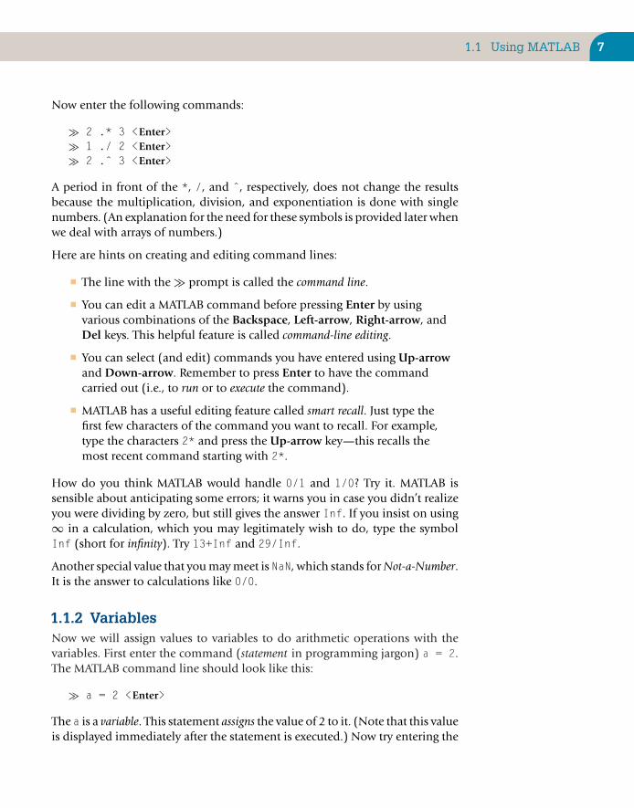
Now enter the following commands:
� 2 .* 3 <Enter>� 1 ./ 2 <Enter>� 2 .ˆ 3 <Enter>
A period in front of the *, /, and ˆ, respectively, does not change the resultsbecause the multiplication, division, and exponentiation is done with singlenumbers. (An explanation for the need for these symbols is provided later whenwe deal with arrays of numbers.)
Here are hints on creating and editing command lines:
■ The line with the � prompt is called the command line.
■ You can edit a MATLAB command before pressing Enter by usingvarious combinations of the Backspace, Left-arrow, Right-arrow, andDel keys. This helpful feature is called command-line editing.
■ You can select (and edit) commands you have entered using Up-arrowand Down-arrow. Remember to press Enter to have the commandcarried out (i.e., to run or to execute the command).
■ MATLAB has a useful editing feature called smart recall. Just type thefirst few characters of the command you want to recall. For example,type the characters 2* and press the Up-arrow key—this recalls themost recent command starting with 2*.
How do you think MATLAB would handle 0/1 and 1/0? Try it. MATLAB issensible about anticipating some errors; it warns you in case you didn’t realizeyou were dividing by zero, but still gives the answer Inf. If you insist on using∞ in a calculation, which you may legitimately wish to do, type the symbolInf (short for infinity). Try 13+Inf and 29/Inf.
Another special value that you may meet is NaN, which stands for Not-a-Number.It is the answer to calculations like 0/0.
1.1.2 VariablesNow we will assign values to variables to do arithmetic operations with thevariables. First enter the command (statement in programming jargon) a = 2.The MATLAB command line should look like this:
� a = 2 <Enter>
The a is a variable. This statement assigns the value of 2 to it. (Note that this valueis displayed immediately after the statement is executed.) Now try entering the

8 CHAPTER 1: Introduction
statement a = a + 7 followed on a new line by a = a * 10. Do you agreewith the final value of a? Do we agree that it is 90?
Now enter the statement
� b = 3; <Enter>
The semicolon (;) prevents the value of b from being displayed. However, bstill has the value 3, as you can see by entering without a semicolon:
� b <Enter>
Assign any values you like to two variables x and y. Now see if you can assignthe sum of x and y to a third variable z in a single statement. One way of doingthis is
� x = 2; y = 3; <Enter>� z = x + y <Enter>
Notice that, in addition to doing the arithmetic with variables with assignedvalues, several commands separated by semicolons (or commas) can be put onone line.
1.1.3 Mathematical functionsMATLAB has all of the usual mathematical functions found on a scientific-electronic calculator, like sin, cos, and log (meaning the natural logarithm).See Appendix C.5 for many more examples.
■ Find√
π with the command sqrt(pi). The answer should be 1.7725.Note that MATLAB knows the value of pi because it is one of its manybuilt-in functions.
■ Trigonometric functions like sin(x) expect the argument x to be inradians. Multiply degrees by π/180 to get radians. For example,use MATLAB to calculate sin(90◦). The answer should be 1(sin(90*pi/180)).
■ The exponential function ex is computed in MATLAB as exp(x). Usethis information to find e and 1/e (2.7183 and 0.3679).
Because of the numerous built-in functions like pi or sin, care must be takenin the naming of user-defined variables. Names should not duplicate thoseof built-in functions without good reason. This problem can be illustrated asfollows:
� pi = 4 <Enter>� sqrt(pi) <Enter>

1.1 Using MATLAB 9
� whos <Enter>� clear pi <Enter>� whos <Enter>� sqrt(pi) <Enter>� clear <Enter>� whos <Enter>
Note that clear executed by itself clears all local variables in the workspace;� clear pi clears the locally defined variable pi. In other words, if you decideto redefine a built-in function or command, the new value is used! The com-mand whos is executed to determine the list of local variables or commandspresently in the workspace. The first execution of the command pi = 4 in theabove example displays your redefinition of the built-in pi: a 1-by-1 (or 1x1)double array, which means this data type was created when pi was assigned anumber (you will learn more about other data types later, as we proceed in ourinvestigation of MATLAB).
1.1.4 Functions and commandsMATLAB has numerous general functions. Try date and calendar for starters.It also has numerous commands, such as clc (for clear command window). helpis one you will use a lot (see below). The difference between functions andcommands is that functions usually return with a value (e.g., the date), whilecommands tend to change the environment in some way (e.g., clearing thescreen or saving some statements to the workspace).
1.1.5 VectorsVariables such asa andb above are called scalars; they are single-valued. MATLABalso handles vectors (generally referred to as arrays), which are the key to manyof its powerful features. The easiest way of defining a vector where the elements(components) increase by the same amount is with a statement like
� x = 0 : 10; <Enter>
That is a colon (:) between the 0 and the 10. There’s no need to leave a spaceon either side of it, except to make it more readable. Enter x to check that x is avector; it is a row vector—consisting of 1 row and 11 columns. Type the followingcommand to verify that this is the case:
� size(x) <Enter>
Part of the real power of MATLAB is illustrated by the fact that other vectors cannow be defined (or created) in terms of the just defined vector x. Try
� y = 2 .* x <Enter>� w = y ./ x <Enter>

10 CHAPTER 1: Introduction
and
� z = sin(x) <Enter>
(no semicolons). Note that the first command line creates a vector y by multi-plying each element of x by the factor 2. The second command line is an arrayoperation, creating a vector w by taking each element of y and dividing it bythe corresponding element of x. Since each element of y is two times the cor-responding element of x, the vector w is a row vector of 11 elements all equalto 2. Finally, z is a vector with sin(x) as its elements.
To draw a reasonably nice graph of sin(x), simply enter the followingcommands:
� x = 0 : 0.1 : 10; <Enter>� z = sin(x); <Enter>� plot(x,z), grid <Enter>
The graph appears in a separate figure window (see Figure 1.2). You can selectthe Command Window or figure windows by clicking anywhere inside them.The Windows pull-down menus can be used in any of them.
Note that the first command line above has three numbers after the equalsign. When three numbers are separated by two colons in this way, the middlenumber is the increment. The increment of 0.1 was selected to give a reasonably
0 1 2 3 4 5 6 7 8 9 1021
20.8
20.6
20.4
20.2
0
0.2
0.4
0.6
0.8
1
FIGURE 1.2Figure window.

1.1 Using MATLAB 11
smooth graph. The command grid following the comma in the last commandline adds a grid to the graph. (The changes in background color were madein the figure window using the figure properties editor, which can be found inthe pull-down menu under Edit in the toolbar. The colors in the figures in thisbook were modified with the figure-editing tools.)
If you want to see more cycles of the sine graph, use command-line editing tochange sin(x) to sin(2*x).
Try drawing the graph of tan(x) over the same domain. You may find aspectsof your graph surprising. A more accurate version is presented in Chapter 5.An alternative way to examine mathematical functions graphically is to use thefollowing command:
� ezplot(’tan(x)’) <Enter>
The apostrophes around the function tan(x) are important in the ezplotcommand. Note that the default domain of x in ezplot is not 0 to 10.
A useful Command Window editing feature is tab completion: Type the firstfew letters of a MATLAB name and then press Tab. If the name is unique, itis automatically completed. If it is not unique, press Tab a second time to seeall the possibilities. Try by typing ta at the command line followed by Tabtwice.
1.1.6 Linear equationsSystems of linear equations are very important in engineering and scien-tific analysis. A simple example is finding the solution to two simultaneousequations:
x + 2y = 4
2x − y = 3
Here are two approaches to the solution.
Matrix method. Type the following commands (exactly as they are):
� a = [1 2; 2 –1]; <Enter>� b = [4; 3]; <Enter>� x = a\b <Enter>
The result is
x =21
i.e., x = 2, y = 1.

12 CHAPTER 1: Introduction
Built-in solve function. Type the following commands (exactly as they are):
� [x,y] = solve(’x+2*y=4’,’2*x–y=3’) <Enter>� whos <Enter>� x = double(x), y=double(y) <Enter>� whos <Enter>
The function double converts x and y from symbolic objects (another datatype in MATLAB) to double arrays (i.e., the numerical-variable data typeassociated with an assigned number).
To check your results, after executing either approach, type the followingcommands (exactly as they are):
� x + 2*y % should give ans = 4 <Enter>� 2*x – y % should give ans = 3 <Enter>
The % symbol is a flag that indicates all information to the right is not part ofthe command but a comment. (We will examine the need for comments whenwe learn to develop coded programs of command lines later on.)
1.1.7 DemoIf you want a spectacular sample of what MATLAB has to offer, try demo at thecommand line. Alternatively, double-click Demos in the Launch Pad, which isfound by clicking the Start button in the lower left-hand corner of the MATLABdesktop. (If you can’t see Demos, click ? to open the Help browser, or launch thedemonstration programs by clicking on Demos in the pull-down menu underHelp.) For a listing of demonstration programs by category try the commandhelp demos.
1.1.8 HelpMATLAB has a very useful Help system, which we will look at in a little moredetail in the last section of this chapter. For the moment type help at thecommand line to see all the Help categories. For example, type help elfun tosee all MATLAB’s elementary mathematical functions. Another utility, lookfor,enables you to search for a particular string in the Help text of functions (e.g.,lookfor eigenvalue displays all functions relating to eigenvalues).
There is one problem with the results that you get in the command window. Thecommands are, for emphasis only, in uppercase; when used they must be typedin lowercase. This is because the latest versions of MATLAB are case sensitive;hence, a and A are considered different names. It is safer and more instructiveto use the Help manuals by clicking ? in the task bar at the top of the MATLABdesktop. The examples are correctly reproduced in the Help manuals found inthe pull-down menu.

1.1 Using MATLAB 13
1.1.9 Additional featuresMATLAB has other good things. For example, you can generate a 10-by-10 (or10 × 10) magic square by executing the command magic(10), where the rows,columns, and main diagonal add up to the same value. Try it. In general, ann × n magic square has a row and column sum of n(n2 + 1)/2.
You can even get a contour plot of the elements of a magic square. MATLABpretends that the elements in the square are heights above sea level of pointson a map, and draws the contour lines. contour(magic(22)) looks nice.
If you want to see the famous Mexican hat (Figure 1.3), enter the following fourlines (be careful not to make any typing errors):
� [x y ] = meshgrid(–8 : 0.5 : 8); <Enter>� r = sqrt(x.ˆ2 + y.ˆ2) + eps; <Enter>� z = sin(r) ./ r; <Enter>� mesh(z); <Enter>
surf(z) generates a faceted (tiled) view of the surface. surfc(z) or meshc(z)draws a 2D contour plot under the surface. The command
3530
2520
1510
50
20.4
20.2
0
0.2
0.4
0.6
0.8
1
05
1015
2025
3035
FIGURE 1.3The Mexican hat.
14 CHAPTER 1: Introduction
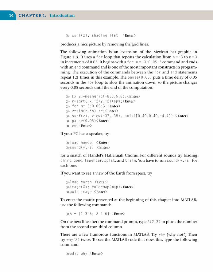
� surf(z), shading flat <Enter>
produces a nice picture by removing the grid lines.
The following animation is an extension of the Mexican hat graphic inFigure 1.3. It uses a for loop that repeats the calculation from n = –3 to n = 3in increments of 0.05. It begins with a for n = –3:0.05:3 command and endswith an end command and is one of the most important constructs in program-ming. The execution of the commands between the for and end statementsrepeat 121 times in this example. The pause(0.05) puts a time delay of 0.05seconds in the for loop to slow the animation down, so the picture changesevery 0.05 seconds until the end of the computation.
� [x y]=meshgrid(–8:0.5:8);<Enter>� r=sqrt( x.ˆ2+y.ˆ2)+eps;<Enter>� for n=–3:0.05:3;<Enter>� z=sin(r.*n)./r;<Enter>� surf(z), view(–37, 38), axis([0,40,0,40,–4,4]);<Enter>� pause(0.05)<Enter>� end<Enter>
If your PC has a speaker, try
�load handel <Enter>�sound(y,Fs) <Enter>
for a snatch of Handel’s Hallelujah Chorus. For different sounds try loadingchirp, gong, laughter, splat, and train. You have to run sound(y,Fs) foreach one.
If you want to see a view of the Earth from space, try
�load earth <Enter>�image(X); colormap(map)<Enter>�axis image <Enter>
To enter the matrix presented at the beginning of this chapter into MATLAB,use the following command:
�A = [1 3 5; 2 4 6] <Enter>
On the next line after the command prompt, type A(2,3) to pluck the numberfrom the second row, third column.
There are a few humorous functions in MATLAB. Try why (why not?) Thentry why(2) twice. To see the MATLAB code that does this, type the followingcommand:
�edit why <Enter>

1.2 The MATLAB Desktop 15
Once you have looked at this file, close it via the pull-down menu by clickingFile at the top of the Editor desktop window and then Close Editor; do notsave the file, in case you accidently typed something and modified it.
The edit command will be used soon to illustrate the creation of an M-file likewhy.m (the name of the file executed by the command why). You will create anM-file after we go over some of the basic features of the MATLAB desktop. Moredetails on creating programs in the MATLAB environment will be explainedwhen the Editor is introduced in Chapter 2.
1.2 THE MATLAB DESKTOP
It should immediately be stressed that MATLAB has an extremely useful onlineHelp system. If you are serious about learning MATLAB, make it your businessto work through the various Help features, starting with the section on thedesktop. The default MATLAB desktop was shown in Figure 1.1.
To get into the Help browser, either click on the Help button (?) on the desktoptoolbar or select the Help menu in any tool. In the Help browser, select the Con-tents tab in the Help Navigator pane on the left. To get to the desktop section,expand successively the Getting Started and Desktop Tools and DevelopmentEnvironment items. Desktop Overview is listed under the latter. Once you’velooked at it, go to Arranging the Desktop. Try some rearranging. (To get backto the default, select the Desktop → Desktop Layout → Default menu item.)
The desktop contains a number of tools. We have already used the CommandWindow. On the left is the Current Directory, which shares a “docking” positionwith the Workspace browser. Use the tabs to switch between the two. Below theCurrent Directory you will find the Command History.
You can resize any of these windows in the usual way. A window can be movedout of the MATLAB desktop by undocking it, either by clicking on the arrow inthe window’s title bar or by making the window active (click anywhere insideit) and then selecting Undock from the Desktop menu. To dock a tool windowthat is outside the MATLAB desktop (i.e., to move it back in), select Dock fromits Desktop menu.
You can group desktop windows so that they occupy the same space. Access tothe individual windows is then by means of their tabs. First drag the title bar ofone window on top of the title bar of the other. The outline of the window you’redragging overlays the target window, and the bottom of the outline includesa tab. The status bar tells you to Release the mouse button to tab-dockthese windows. If you release the mouse, the windows are duly tab-docked inthe outlined position.
There are six predefined MATLAB desktop configurations, which you can selectfrom Desktop → Desktop Layout.

16 CHAPTER 1: Introduction
1.3 SAMPLE PROGRAM
In Section 1.1 we saw some simple examples of how to use MATLAB by enteringsingle commands or statements at the MATLAB prompt. However, you mightwant to solve problems that MATLAB can’t do in one line, like finding theroots of a quadratic equation (and taking all the special cases into account).A collection of statements to solve such a problem is called a program. In thissection we look at the mechanics of writing and running two short programs,without bothering too much about how they work—explanations will followin Chapter 2.
1.3.1 Cut and pasteSuppose you want to draw the graph of e−0.2x sin(x) over the domain 0 to 6π,as shown in Figure 1.4. The Windows environment lends itself to cut and pasteediting, which you would do well to master.
From the MATLAB desktop select File → New → M-file, or click the New Filebutton on the desktop toolbar. (You could also type edit in the CommandWindow followed by Enter.) This action opens an “Untitled” window in theEditor/Debugger. For the time being you can regard this as a “scratch pad” onwhich to write programs. Now type the following two lines in the Editor, exactlyas they appear here:
x = 0 : pi/20 : 6 * pi;plot(x, exp(–0.2*x) .* sin(x), ’k’),grid
0 2 4 6 8 10 12 14 16 18 2020.4
20.2
0
0.2
0.4
0.6
0.8
1
FIGURE 1.4e−0.2x sin(x).

1.3 Sample Program 17
Incidentally, that is a dot (period) in front of the second * in the second line—a more detailed explanation later. The additional argument ’k’ for plot willdraw a black graph, just to be different. Change ’k’ to ’r’ to generate a redgraph.
Next move the cursor (which now looks like a very thin capital I) to the leftof the x in the first line. Keep the left mouse button down while moving thepointer to the end of the second line. This is called dragging. Both lines shouldbe highlighted at this stage, probably in blue, to indicate that they have beenselected.
Select the Edit menu in the Editor window, and click Copy (or use the key-board shortcut Ctrl+C). This action copies the highlighted text to the clipboard(assuming that your operating system is Windows).
Now go back to the Command Window. Make sure the cursor is positioned atthe � prompt (click there if necessary). Select the Edit menu, and click Paste(or use the Ctrl+V shortcut). The contents of the clipboard will be copied intothe Command Window. To execute the two lines in the program, press Enter.The graph should appear in a figure window.
This process, from highlighting (selecting) text in the Editor to copying it intothe Command Window, is called cut and paste (more correctly “copy and paste”here, since the original text is copied from the Editor rather than cut from it).It is well worth practicing until you have it right.
If you need to correct the program, go back to the Editor, click at the position ofthe error (this moves the insertion point to the right place), make the correction,and cut and paste again. Alternatively, use command-line editing to correctmistakes, or paste from the Command History window (which incidentally goesback over many previous sessions). To select multiple lines in the CommandHistory window, keep Ctrl down while you click.
If you prefer, you can enter multiple lines directly in the Command Window.To prevent the entire group from running until you have entered the last line,use Shift+Enter or Ctrl+Enter after each line until the last. Then press Enter torun all of them.
Suppose you have $1000 saved in the bank, with interest is compounded at therate of 9% per year. What will your bank balance be after one year? If you wantto write a MATLAB program to find your new balance, you must be able to dothe problem yourself in principle. Thus, even with a relatively simple problemlike this, it often helps first to write down a rough structure plan:
1. Get the data (initial balance and interest rate) into MATLAB2. Calculate the interest (9% of $1000, i.e., $90)3. Add the interest to the balance ($90 + $1000, i.e., $1090)4. Display the new balance

18 CHAPTER 1: Introduction
Go back to the Editor. To clear out any previous text, select it as usual by dragging(or use Ctrl+A) and press the Del key. (By the way, to deselect highlighted text,click anywhere outside the selection area.) Enter the following program, andthen cut and paste it to the Command Window.
balance = 1000;rate = 0.09;interest = rate * balance;balance = balance + interest;disp( ’New balance:’ );disp( balance );
When you press Enter, you should get the following output:
New balance:1090
1.3.2 Saving a program: script filesWe have seen how to cut and paste between the Editor and the CommandWindow in order to write and run MATLAB programs. Obviously you need tosave the program if you want to use it again later.
To save the contents of the Editor, select File → Save from the Editor menubar. Under Save file as, select a directory and enter a filename, which must havethe extension .m, in the File name: box (e.g., junk.m). Click Save. The Editorwindow now has the title junk.m. If you make subsequent changes to junk.m,an asterisk appears next to its name at the top of the Editor until you save thechanges.
A MATLAB program saved from the Editor (or any ASCII text editor) with theextension .m is called a script file, or simply a script. (MATLAB function filesalso have the extension .m. We therefore refer to both script and function filesgenerally as M-files.) The special significance of a script file is that, if you enterits name at the command-line prompt, MATLAB carries out each statement init as if it were entered at the prompt.
The rules for script file names are the same as those for MATLAB variable names(see Section 2.1).
As an example, save the compound interest program above in a script file underthe name compint.m. Then simply enter the name
compint
at the Command Window prompt and hit Enter. The statements in compint.mwill be carried out exactly as if you had pasted them into the Command Window.You have effectively created a new MATLAB command, compint.

1.3 Sample Program 19
A script file may be listed in the Command Window with the command type:
type compint
(the extension .m may be omitted).
Script files provide a useful way of managing large programs that you do notnecessarily want to paste into the Command Window every time you run them.
Current DirectoryWhen you run a script, make sure that MATLAB’s Current Directory (indicatedin the Current Directory field on the right of the desktop toolbar) is set to thedirectory in which the script is saved. To change the Current Directory, type thepath for the new one in the Current Directory field, or select from the drop-down list of previous working directories or click on the browse button (…).
The Current Directory may be changed in this way from the Current Directorybrowser in the desktop. You can also change it from the command line withthe cd command:
cd \mystuff
cd by itself returns the name of the Current Directory.
Running a script from the Current Directory browserA handy way to run a script is as follows. Right-click the file in the CurrentDirectory browser. The context menu appears (context menus are a general fea-ture of the desktop); select Run from it. The results appear in the CommandWindow. If you want to edit the script, select Open from the context menu.
The Help portion of an M-file appears in the pane at the bottom of the CurrentDirectory browser. Try this with an M-file in one of the MATLAB directories(e.g., \toolbox\matlab\elmat). A one-line description of the file appears inthe rightmost column (you may need to enlarge the browser to see all columns).
1.3.3 A program in actionWe will now discuss in detail how the compound interest program works.
The MATLAB system is technically called an interpreter (as opposed to acompiler). This means that each statement presented to the command lineis translated (interpreted) into language the computer understands and isimmediately carried out.
A fundamental concept in MATLAB is how numbers are stored in the computer’srandom access memory (RAM). If a MATLAB statement needs to store a number,RAM space is set aside for it. You can think of this space as a bank of boxes

20 CHAPTER 1: Introduction
or memory locations, each of which can hold only one number at a time. Eachmemory location is referred to by a symbolic name in MATLAB, so the statement
balance = 1000
allocates the number 1000 to the memory location named balance. Since itscontents may change during a session, balance is called a variable.
The statements in our program are therefore interpreted by MATLAB asfollows:
1. Put the number 1000 into variable balance.
2. Put the number 0.09 into variable rate.
3. Multiply the contents of rate by the contents of balance and put theanswer in interest.
4. Add the contents of balance to the contents of interest and put theanswer in balance.
5. Display (in the Command Window) the message given in apostrophes.
6. Display the contents of balance.
It hardly seems necessary to stress this, but interpreted statements are carriedout in top-down order. When the program has finished running, the variablesused will have the following values:
balance : 1090interest : 90rate : 0.09
Note that the original value of balance (1000) is lost.
EXERCISES
1. Run the compound interest program as it stands.
2. Change the first statement in the program to read
balance = 2000;Make sure that you understand what happens when the program runs.
3. Leave out the line
balance = balance + interest;and rerun. Can you explain what happens?
4. Rewrite the program so that the original value of balance is not lost.

Summary 21
A number of questions have probably occurred to you by now, such as
■ What names may be used for variables?
■ How can numbers be represented?
■ What happens if a statement won’t fit on one line?
■ How can we organize the output more neatly?
These will be answered in Chapter 2, which will also introduce some additionalbasic concepts.
SUMMARY
■ MATLAB is a matrix-based computer system designed for scientific andengineering problem solving.
■ In MATLAB, commands and statements are entered on the command linein the Command Window. They are carried out immediately.
■ quit or exit terminates MATLAB.
■ clc clears the Command Window.
■ help and lookfor provide help.
■ plot draws an x-y graph in a figure window.
■ grid draws grid lines on a graph.
CHAPTER EXERCISES
1.1. Give values to variables a and b on the command line—for example, a = 3 and b = 5.Write statements to find the sum, difference, product, and quotient of a and b.
1.2. Section 1.1 gives a script for animating the Mexican hat problem. Type this into theeditor, save it, and execute it. Once you finish debugging it and it executes successfully,try modifying it.(a) Change the maximum value of n from 3 to 4 and execute the script.
(b) Change the time delay in the pause function from 0.05 to 0.1.
(c) Change the z = sin(r.*n)./r; command line to z = cos(r.*n); andexecute the script.
Solutions to many of the exercises in this and subsequent chapters are given inAppendix E.
CHAPTER 2
MATLAB Fundamentals
The objective of this chapter is to introduce some of the fundamentals ofMATLAB programming, including:
■ Variables, operators, and expressions■ Arrays (including vectors and matrices)■ Basic input and output■ Repetition (for)■ Decisions (if)
The tools introduced in this chapter are sufficient to begin solving numerousscientific and engineering problems you may encounter in your course work andin your profession. The last part of this chapter and the next chapter describean approach to designing reasonably good programs to initiate the building oftools for your own toolbox.
2.1 VARIABLES
Variables are fundamental to programming. In a sense, the art of programmingis this:
Getting the right values in the right variables at the right time
A variable name (like the variable balance that we used in Chapter 1) mustcomply with the following two rules:
■ It may consist only of the letters a–z, the digits 0–9, and theunderscore ( _ ).
■ It must start with a letter.Copyright © 2010, Daniel T. Valentine. Published by Elsevier Ltd. All rights reserved.DOI: 10.1016/B978-0-12-374883-6.00002-3 23

24 CHAPTER 2: MATLAB Fundamentals
The name may be as long as you like, but MATLAB only remembers the first 63characters (to check this on your version, execute the commandnamelengthmaxin the Command Window of the MATLAB desktop). Examples of valid vari-able names are r2d2 and pay_day. Examples of invalid names (why?) arepay-day, 2a, name$, and _2a.
A variable is created simply by assigning a value to it at the command line orin a program—for example,
a = 98
If you attempt to refer to a nonexistent variable you will get the error message
??? Undefined function or variable ...
The official MATLAB documentation refers to all variables as arrays, whetherthey are single-valued (scalars) or multi-valued (vectors or matrices). In otherwords, a scalar is a 1-by-1 array—an array with a single row and a single columnwhich, of course, is an array of one item.
2.1.1 Case sensitivityMATLAB is case-sensitive, which means it distinguishes between upper- andlowercase letters. Thus, balance, BALANCE and BaLance are three differentvariables. Many programmers write variable names in lowercase except for thefirst letter of the second and subsequent words, if the name consists of morethan one word run together. This style is known as camel caps, the uppercaseletters looking like a camel’s humps (with a bit of imagination). Examplesare camelCaps, milleniumBug, dayOfTheWeek. Some programmers prefer toseparate words with underscores.
Command and function names are also case-sensitive. However, note that whenyou use the command-line help, function names are given in capitals (e.g., CLC)solely to emphasize them. You must not use capitals when running functionsand commands!
2.2 THE WORKSPACE
Another fundamental concept in MATLAB is the workspace. Enter the commandclear and then rerun the compound interest program (see Section 1.3.2). Nowenter the command who. You should see a list of variables as follows:
Your variables are:
balance interest rate

2.2 The Workspace 25
All the variables you create during a session remain in the workspace until youclear them. You can use or change their values at any stage during the session.The command who lists the names of all the variables in your workspace. Thefunction ans returns the value of the last expression evaluated but not assignedto a variable. The command whos lists the size of each variable as well:
Name Size Bytes Class
balance 1x1 8 double arrayinterest 1x1 8 double arrayrate 1x1 8 double array
Each variable here occupies eight bytes of storage. A byte is the amount of com-puter memory required for one character (if you are interested, one byte is thesame as eight bits). These variables each have a size of “1 by 1,” because theyare scalars, as opposed to vectors or matrices (although as mentioned above,MATLAB regards them all as 1-by-1 arrays).
double means that the variable holds numeric values as double-precisionfloating-point (see Section 2.5).
The command clear removes all variables from the workspace. A particularvariable can be removed from the workspace (e.g., clear rate). More thanone variable can also be cleared (e.g., clear rate balance). Separate thevariable names with spaces, not commas.
When you run a program, any variables created by it remain in the workspaceafter it runs. This means that existing variables with the same names areoverwritten.
The Workspace browser on the desktop provides a handy visual representationof the workspace. You can view and even change the values of workspace vari-ables with the Array Editor. To activate the Array Editor click on a variable in theWorkspace browser or right-click to get the more general context menu. Fromthe context menu you can draw graphs of workspace variables in various ways.
2.2.1 Adding commonly used constants to the workspaceIf you often use the same physical or mathematical constants in your MATLABsessions, you can save them in an M-file and run the file at the start of a session.For example, the following statements can be saved in myconst.m:
g = 9.8; % acceleration due to gravityavo = 6.023e23; % Avogadro’s numbere = exp(1); % base of natural logpi_4 = pi / 4;log10e = log10( e );bar_to_kP = 101.325; % atmospheres to kiloPascals

26 CHAPTER 2: MATLAB Fundamentals
If you run myconst at the start of a session, these six variables will be part of theworkspace and will be available for the rest of the session or until you clearthem. This approach to using MATLAB is like a notepad (it is one of many ways).As your experience grows, you will discover many more utilities and capabilitiesassociated with MATLAB’s computational and analytical environment.
2.3 ARRAYS: VECTORS AND MATRICES
As mentioned in Chapter 1, the name MATLAB stands for Matrix Laboratorybecause MATLAB has been designed to work with matrices. A matrix is a rect-angular object (e.g., a table) consisting of rows and columns. We will postponemost of the details of proper matrices and how MATLAB works with them untilChapter 6.
A vector is a special type of matrix, having only one row or one column. Vectorsare called lists or arrays in other programming languages. If you haven’t comeacross vectors officially yet, don’t worry—just think of them as lists of numbers.
MATLAB handles vectors and matrices in the same way, but since vectors areeasier to think about than matrices, we will look at them first. This will enhanceyour understanding and appreciation of many aspects of MATLAB. As men-tioned above, MATLAB refers to scalars, vectors, and matrices generally as arrays.We will also use the term array generally, with vector and matrix referring to theone-dimensional (1D) and two-dimensional (2D) array forms.
2.3.1 Initializing vectors: Explicit listsAs a start, try the accompanying short exercises on the command line. These areall examples of the explicit list method of initializing vectors. (You won’t needreminding about the command prompt � any more, so it will no longer appearunless the context absolutely demands it.)
EXERCISES
2.1. Enter a statement like
x = [1 3 0 –1 5]
Can you see that you have created a vector (list) with five elements? (Make sure to leaveout the semicolon so that you can see the list. Also, make sure you hit Enter to executethe command.)
2.2. Enter the command disp(x) to see how MATLAB displays a vector.
2.3. Enter the command whos (or look in the Workspace browser). Under the heading Sizeyou will see that x is 1 by 5, which means 1 row and 5 columns. You will also see thatthe total number of elements is 5.

2.3 Arrays: Vectors and Matrices 27
2.4. You can use commas instead of spaces between vector elements if you like. Try this:
a = [5,6,7]
2.5. Don’t forget the commas (or spaces) between elements; otherwise, you could end upwith something quite different:
x = [130–15]
What do you think this gives?
2.6. You can use one vector in a list for another one. Type in the following:
a = [1 2 3];b = [4 5];c = [a –b];
Can you work out what c will look like before displaying it?
2.7. And what about this?
a = [1 3 7];a = [a 0 –1];
2.8. Enter the following
x = [ ]
Note in the Workspace browser that the size of x is given as 0 by 0 because x is empty .This means x is defined and can be used where an array is appropriate without causingan error; however, it has no size or value.
Making x empty is not the same as saying x = 0 (in the latter case x has size 1 by 1) orclear x (which removes x from the workspace, making it undefined).
An empty array may be used to remove elements from an array (see Section 2.3.5).
Remember the following important rules:
■ Elements in the list must be enclosed in square brackets, notparentheses.
■ Elements in the list must be separated either by spaces or by commas.
2.3.2 Initializing vectors: The colon operatorA vector can also be generated (initialized) with the colon operator, as we saw inChapter 1. Enter the following statements:
x = 1:10
(elements are the integers 1, 2, … , 10)
x = 1:0.5:4
(elements are the values 1, 1.5, … , 4 in increments of 0.5. Note that if thecolons separate three values, the middle value is the increment);

28 CHAPTER 2: MATLAB Fundamentals
x = 10:–1:1
(elements are the integers 10, 9, … , 1, since the increment is negative);
x = 1:2:6
(elements are 1, 3, 5; note that when the increment is positive but not equal to1, the last element is not allowed to exceed the value after the second colon);
x = 0:–2:–5
(elements are 0, −2, −4; note that when the increment is negative but not equalto −1, the last element is not allowed to be less than the value after the secondcolon);
x = 1:0
(a complicated way of generating an empty vector!).
2.3.3 The linspace functionThe function linspace can be used to initialize a vector of equally spacedvalues:
linspace(0, pi/2, 10)
creates a vector of 10 equally spaced points from 0 to π/2 (inclusive).
2.3.4 Transposing vectorsAll of the vectors examined so far are row vectors. Each has one row and severalcolumns. To generate the column vectors that are often needed in mathematics,you need to transpose such vectors—that is, you need to interchange their rowsand columns. This is done with the single quote, or apostrophe (’), which isthe nearest MATLAB can get to the mathematical prime (′) that is often used toindicate the transpose.
Enter x = 1:5 and then enter x’ to display the transpose of x. Note that x itselfremains a row vector. Alternatively, or you can create a column vector directly:
y = [1 4 8 0 –1]’
2.3.5 SubscriptsWe can refer to particular elements of a vector by means of subscripts. Try thefollowing:
1. Enter r = rand(1,7). This gives you a row vector of seven randomnumbers.
2.3 Arrays: Vectors and Matrices 29
2. Enter r(3). This will display the third element of r. The numeral 3 is thesubscript.
3. Enter r(2:4). This should give you the second, third, and fourthelements.
4. What about r(1:2:7) and r([1 7 2 6])?
5. Use an empty vector to remove elements from a vector:
r([1 7 2]) = [ ]
This will remove elements 1, 7, and 2.
To summarize:
■ A subscript is indicated by parentheses.
■ A subscript may be a scalar or a vector.
■ In MATLAB subscripts always start at 1.
■ Fractional subscripts are not allowed.
2.3.6 MatricesA matrix may be thought of as a table consisting of rows and columns. You createa matrix just as you do a vector, except that a semicolon is used to indicate theend of a row. For example, the statement
a = [1 2 3; 4 5 6]
results in
a =1 2 34 5 6
A matrix may be transposed: With a initialized as above, the statement a’results in
a =1 42 53 6
A matrix can be constructed from column vectors of the same length. Thus, thestatements
x = 0:30:180;table = [x’ sin(x*pi/180)’]

30 CHAPTER 2: MATLAB Fundamentals
result in
table =0 0
30.0000 0.500060.0000 0.866090.0000 1.0000120.0000 0.8660150.0000 0.5000180.0000 0.0000
2.3.7 Capturing outputYou can use cut and paste techniques to tidy up the output from MATLABstatements if this is necessary for some sort of presentation. Generate the tableof angles and sines as shown above. Select all seven rows of numerical outputin the Command Window, and copy the selected output to the Editor. Youcan then edit the output, for example, by inserting text headings above eachcolumn (this is easier than trying to get headings to line up over the columnswith a disp statement). The edited output can in turn be pasted into a reportor printed as is (the File menu has a number of printing options).
Another way of capturing output is with the diary command. The command
diary filename
copies everything that subsequently appears in the Command Window tothe text file filename. You can then edit the resulting file with any text editor(including the MATLAB Editor). Stop recording the session with
diary off
Note that diary appends material to an existing file—that is, it adds newinformation to the end of it.
2.4 VERTICAL MOTION UNDER GRAVITY
If a stone is thrown vertically upward with an initial speed u, its vertical dis-placement s after an elapsed time t is given by the formula s = ut − gt2/2, whereg is the acceleration due to gravity. Air resistance is ignored. We would like tocompute the value of s over a period of about 12.3 seconds at intervals of0.1 seconds, and plot the distance–time graph over this period, as shown inFigure 2.1. The structure plan for this problem is as follows:
1. % Assign the data (g, u, and t) to MATLAB variables2. % Calculate the value of s according to the formula

2.4 Vertical Motion Under Gravity 31
0 4 6 82 12 1410250
0
50
100
150
200
Time
Vertical motion under gravity
Ver
tical
dis
plac
emen
t
FIGURE 2.1Distance-time graph of a stone thrown vertically upward.
3. % Plot the graph of s against t4. % Stop
This plan may seem trivial and a waste of time to write down. Yet you would besurprised how many beginners, preferring to rush straight to the computer, startwith step 2 instead of step 1. It is well worth developing the mental disciplineof structure-planning your program first. You can even use cut and paste to planas follows:
1. Type the structure plan into the Editor (each line preceeded by % asshown above).
2. Paste a second copy of the plan directly below the first.
3. Translate each line in the second copy into a MATLAB statement orstatements (add % comments as in the example below).
4. Finally, paste all the translated MATLAB statements into the CommandWindow and run them.
5. If necessary, go back to the Editor to make corrections and repaste thecorrected statements to the Command Window (or save the program inthe Editor as an M-file and execute it).
You might like to try this as an exercise before looking at the final program,which is as follows:
% Vertical motion under gravityg = 9.81; % acceleration due
% to gravityu = 60; % initial velocity in
% metres/sec

32 CHAPTER 2: MATLAB Fundamentals
t = 0 : 0.1 : 12.3; % time in secondss = u * t – g / 2 * t .ˆ 2; % vertical displacement
% in metresplot(t, s), title( ’Vertical motion under gravity’ )xlabel( ’time’ ), ylabel( ’vertical displacement’ )griddisp( [t’ s’] ) % display a table
The graphical output is shown in Figure 2.1.
Note the following points:
■ Anything in a line following the symbol % is ignored by MATLAB andmay be used as a comment (description).
■ The statement t = 0 : 0.1 : 12.3 sets up a vector.
■ The formula for s is evaluated for every element of the vector t, makinganother vector.
■ The expression t.ˆ2 squares each element in t. This is called an arrayoperation and is different from squaring the vector itself, which is amatrix operation, as we will see later.
■ More than one statement can be entered on the same line if thestatements are separated by commas.
■ A statement or group of statements can be continued to the next linewith an ellipsis of three or more dots (...).
■ The statement disp([t’ s’]) first transposes the row vectors t and sinto two columns and constructs a matrix from them, which is thendisplayed.
You might want to save the program under a helpful name, like throw.m, ifyou think you might come back to it. In that case, it would be worth keepingthe structure plan as part of the file; just insert % symbols in front of each line.This way, the plan reminds you what the program does when you look at itagain after some months. Note that you can use the context menu in the Editorto Comment/Uncomment a block of selected text. After you block selectedtext, right-click to see the context menu. To comment the text, scroll down toComment, point, and click.
2.5 OPERATORS, EXPRESSIONS, AND STATEMENTS
Any program worth its salt actually does something. What it basically does isevaluate expressions, such as
2.5 Operators, Expressions, and Statements 33
u*t – g/2*t.ˆ2
and execute (carry out) statements, such as
balance = balance + interest
MATLAB is described as an expression based language because it interpretsand evaluates typed expressions. Expressions are constructed from a varietyof things, such as numbers, variables, and operators. First we need to look atnumbers.
2.5.1 NumbersNumbers can be represented in MATLAB in the usual decimal form (fixed point)with an optional decimal point,
1.2345 –123 .0001
They may also be represented in scientific notation. For example, 1.2345 × 10⁹
may be represented in MATLAB as 1.2345e9. This is also called floating-pointnotation. The number has two parts: the mantissa, which may have an optionaldecimal point (1.2345 in this example) and the exponent (9), which must bean integer (signed or unsigned). Mantissa and exponent must be separated bythe letter e (or E). The mantissa is multiplied by the power of 10 indicated bythe exponent.
Note that the following is not scientific notation: 1.2345*10ˆ9. It is actuallyan expression involving two arithmetic operations (* and ˆ) and therefore moretime consuming. Use scientific notation if the numbers are very small or verylarge, since there’s less chance of making a mistake (e.g., represent 0.000000001as 1e-9).
On computers using standard floating-point arithmetic, numbers are repre-sented to approximately 16 significant decimal digits. The relative accuracy ofnumbers is given by the function eps, which is defined as the distance between1.0 and the next largest floating-point number. Enter eps to see its value onyour computer.
The range of numbers is roughly ±10−308 to ±10308. Precise values for yourcomputer are returned by the MATLAB functions realmin and realmax.
As an exercise, enter the following numbers at the command prompt in scientificnotation (answers follow in parentheses):
1.234 × 10⁵, −8.765 × 10⁻⁴, 10−15, −1012
(1.234e5, –8.765e–4, 1e–15, –1e12)

34 CHAPTER 2: MATLAB Fundamentals
2.5.2 Data typesMATLAB has 14 fundamental data types (or classes). The default numeric datatype is double precision; all MATLAB computations are in double precision.More information on data types can be found in the Help index.
MATLAB also supports signed and unsigned integer types and single-precisionfloating-point, by means of functions such as int8, uint8, single, and the like.However, before mathematical operations can be performed on such types, theymust be converted to double precision using the double function.
2.5.3 Arithmetic operatorsThe evaluation of expressions is achieved by means of arithmetic operators.The arithmetic operations on two scalar constants or variables are shown inTable 2.1. Operators operate on operands (a and b in the table).
Left division seems a little curious: Divide the right operand by the left operand.For scalar operands the expressions 1/3 and 3\1 have the same numerical value(a colleague of mine speaks of the latter as “3 under 1”). However, matrix leftdivision has an entirely different meaning, as we will see later.
2.5.4 Operator precedenceSeveral operations may be combined in one expression—for example,g * t ˆ 2. MATLAB has strict precedence rules for which operations are per-formed first in such cases. The precedence rules for the operators in Table 2.1 areshown in Table 2.2. Note that parentheses have the highest precedence. Notealso the difference between parentheses and square brackets. The former areused to alter the precedence of operators and to denote subscripts, while thelatter are used to create vectors.
When operators in an expression have the same precedence, the operations arecarried out from left to right. So a / b * c is evaluated as (a / b) * c andnot as a / (b * c).
Table 2.1 Arithmetic Operations betweenTwo Scalars
Operation Algebraic form MATLAB
Addition a + b a + bSubtraction a − b a – bMultiplication a × b a * bRight division a/b a / bLeft division b/a a \ bPower ab a ˆ b

2.5 Operators, Expressions, and Statements 35
Table 2.2 Precedence of Arithmetic Operator
Precedence Operator
1 Parentheses2 Power, left to right3 Multiplication and division, left to right4 Addition and subtraction, left to right
EXERCISES
2.1. Evaluate the following MATLAB expressions yourself before checking the answers inMATLAB:
1 + 2 * 34 / 2 * 21+2 / 41 + 2\42*2 ˆ 32 * 3 \ 32 ˆ (1 + 2)/31/2e–1
2.2. Use MATLAB to evaluate the following expressions. Answers are in parentheses.
(a)1
2 × 3(0.1667)
(b) 22×3 (64)
(c) 1.5 × 10⁻⁴ + 2.5 × 10⁻² (0.0252; use scientific or floating-point notation)
2.5.5 The colon operatorThe colon operator has a lower precedence than the plus operator, as thefollowing shows:
1+1:5
The addition is carried out first and a vector with elements 2, … , 5 is theninitialized.
You may be surprised at the following:
1+[1:5]
Were you? The value 1 is added to each element of the vector 1:5. In this context,the addition is called an array operation because it operates on each element ofthe vector (array). Array operations are discussed below.

36 CHAPTER 2: MATLAB Fundamentals
See Appendix B for a complete list of MATLAB operators and their precedences.
2.5.6 The transpose operatorThe transpose operator has the highest precedence. Try
1:5’
The 5 is transposed first (into itself since it is a scalar!), and then a row vectoris formed. Use square brackets if you want to transpose the whole vector:
[1:5]’
2.5.7 Arithmetic operations on arraysEnter the following statements at the command line:
a = [2 4 5];b = [6 2 2];a .* ba ./ b
MATLAB has four additional arithmetic operators, as shown in Table 2.3 thatwork on corresponding elements of arrays with equal dimensions. They aresometimes called array or element-by-element operations because they are per-formed element by element. For example, a .* b results in the following vector(sometimes called the array product):
[a(1)*b(1) a(2)*b(2) a(3)*b(3)]
that is, [6 8 10].
You will have seen that a ./ b gives element-by-element division. Now try[2 3 4] .ˆ [4 3 1]. The ith element of the first vector is raised to the powerof the ith element of the second vector. The period (dot) is necessary for thearray operations of multiplication, division, and exponentiation because theseoperations are defined differently for matrices; they are then called matrix oper-ations (see Chapter 6). With a and b as defined above, try a + b and a - b. For
Table 2.3 Arithmetic Operators forElement-by-Element Arrays
Operator Description
.* Multiplication
./ Right division
.\ Left division
.ˆ Power

2.5 Operators, Expressions, and Statements 37
addition and subtraction, array operations and matrix operations are the same,so we don’t need the period to distinguish them.
When array operations are applied to two vectors, both vectors must be thesame size!
Array operations also apply between a scalar and a nonscalar. Check this with3 .* a and a .ˆ 2. This property is called scalar expansion. Multiplicationand division operations between scalars and nonscalars can be written with orwithout the period (i.e., if a is a vector, 3 .* a is the same as 3 * a).
A common application of element-by-element multiplication is finding thescalar product (also called the dot product) of two vectors x and y, which isdefined as
x · y =∑
i
xiyi
The MATLAB function sum(z) finds the sum of the elements of the vector z,so the statement sum(a .* b) will find the scalar product of a and b (30 for aand b defined above).
EXERCISES
Use MATLAB array operations to do the following:
2.1. Add 1 to each element of the vector [2 3 –1].
2.2. Multiply each element of the vector [1 4 8] by 3.
2.3. Find the array product of the two vectors [1 2 3] and [0 –1 1]. (Answer:[0 –2 3])
2.4. Square each element of the vector [2 3 1].
2.5.8 ExpressionsAn expression is a formula consisting of variables, numbers, operators, and func-tion names. It is evaluated when you enter it at the MATLAB prompt. Forexample, evaluate 2π as follows:
2 * pi
MATLAB’s response is
ans =6.2832
Note that MATLAB uses the function ans (which stands for answer) to returnthe last expression to be evaluated but not assigned to a variable.

38 CHAPTER 2: MATLAB Fundamentals
If an expression is terminated with a semicolon (;), its value is not displayed,although it is still returned by ans.
2.5.9 StatementsMATLAB statements are frequently of the form
variable = expression
as in
s = u * t – g / 2 * t .ˆ 2;
This is an example of an assignment statement because the value of the expres-sion on the right is assigned to the variable (s) on the left. Assignment alwaysworks in this direction. Note that the object on the left-hand side of the assign-ment must be a variable name. A common mistake is to get the statement thewrong way around, as in
a + b = c
Basically any line that you enter in the Command Window or in a program,which MATLAB accepts, is a statement, so a statement can be an assignment, acommand, or simply an expression, such as
x = 29; % assignmentclear % commandpi/2 % expression
This naming convention is in keeping with most programming languages andserves to emphasize the different types of statements that are found in pro-gramming. However, the MATLAB documentation tends to refer to all of theseas “functions.”
As we have seen, a semicolon at the end of an assignment or expressionsuppresses any output. This is useful for suppressing irritating output ofintermediate results (or large matrices).
A statement that is too long to fit on one line may be continued to the next linewith an ellipsis of at least three dots:
x = 3 * 4 – 8 ..../ 2 ˆ 2;
Statements on the same line may be separated by commas (output notsuppressed) or semicolons (output suppressed):
a = 2; b = 3, c = 4;

2.5 Operators, Expressions, and Statements 39
Note that the commas and semicolons are not technically part of the statements;they are separators.
Statements may involve array operations, in which case the variable on theleft-hand side may become a vector or a matrix.
2.5.10 Statements, commands, and functionsThe distinction between MATLAB statements, commands, and functions can bea little fuzzy, since all can be entered on the command line. However, it ishelpful to think of commands as changing the general environment in someway, for example, load, save, and clear. Statements do the sort of thing weusually associate with programming, such as evaluating expressions and car-rying out assignments, making decisions (if), and repeating (for). Functionsreturn with calculated values or perform some operation on data, such as sinand plot.
2.5.11 Formula vectorizationWith array operations, you can easily evaluate a formula repeatedly for a largeset of data. This is one of MATLAB’s most useful and powerful features, and youshould always look for ways to exploit it.
Let us again consider, as an example, the calculation of compound interest. Anamount of money A invested over a period of years n with an annual interest rater grows to an amount A(1 + r)n. Suppose we want to calculate final balancesfor investments of $750, $1000, $3000, $5000, and $11,999 over 10 years withan interest rate of 9%. The following program (comp.m) uses array operationson a vector of initial investments to do this:
format bankA = [750 1000 3000 5000 11999];r = 0.09;n = 10;B = A * (1 + r) ˆ n;disp( [A’ B’] )
The output is
750.00 1775.521000.00 2367.363000.00 7102.095000.00 11836.82
11999.00 28406.00

40 CHAPTER 2: MATLAB Fundamentals
Note the following:
■ In the statement B = A * (1 + r) ˆ n, the expression (1 + r) ˆ nis evaluated first because exponentiation has a higher precedence thanmultiplication.
■ Each element of the vector A is then multiplied by the scalar(1 + r) ˆ n (scalar expansion).
■ The operator * may be used instead of .* because the multiplication isbetween a scalar and a nonscalar (although .* would not cause an errorbecause a scalar is a special case of an array).
■ A table is displayed whose columns are given by the transposes of Aand B.
This process is called formula vectorization. The operation in the statementdescribed in bullet item 1 is such that every element in the vector B is deter-mined by operating on every element of vector A all at once, by interpretingonce a single command line.
See if you can adjust the program comp.m to find the balances for a singleamount A ($1000) over 1, 5, 10, 15, and 20 years. (Hint: use a vector for n:[1 5 10 15 20].)
EXERCISES
2.1. Evaluate the following expressions yourself (before you use MATLAB to check). Thenumerical answers are in parentheses.(a) 2 / 2 * 3 (3)
(b) 2 / 3 ˆ 2 (2/9)
(c) (2 / 3) ˆ 2 (4/9)
(d) 2 + 3 * 4 – 4 (10)
(e) 2 ˆ 2 * 3 / 4 + 3 (6)
(f) 2 ˆ (2 * 3) / (4 + 3) (64/7)
(g) 2 * 3 + 4 (10)
(h) 2 ˆ 3 ˆ 2 (64)
(i) –4 ˆ 2 (–16; ˆ has higher precedence than –)
2.2. Use MATLAB to evaluate the following expressions. The answers are in parentheses.(a)
√2 (1.4142; use sqrt or ˆ0.5)
(b)3 + 45 + 6
(0.6364; use brackets)
(c) Find the sum of 5 and 3 divided by their product (0.5333)
(d) 232(512)
(e) Find the square of 2π (39.4784; use pi)
(f) 2π2 (19.7392)

2.5 Operators, Expressions, and Statements 41
(g) 1/√
2π (0.3989)
(h)1
2√
π(0.2821)
(i) Find the cube root of the product of 2.3 and 4.5 (2.1793)
(j)1 − 2
3+2
1 + 23−2
(0.2)
(k) 1000(1 + 0.15/12)60 (2107.2—for example, $1000 deposited for 5 years at 15%per year, with the interest compounded monthly)
(l) (0.0000123 + 5.678 × 10−3) × 0.4567 × 10−4 (2.5988 × 10⁻⁷; use scientificnotation—for example, 1.23e–5 … ; do not use ˆ)
2.3. Try to avoid using unnecessary brackets in an expression. Can you spot the errors inthe following expression? (Test your corrected version with MATLAB.)
(2(3+4)/(5*(6+1))ˆ2
Note that the MATLAB Editor has two useful ways of dealing with the problem of“unbalanced delimiters” (which you should know about if you have been workingthrough Help!):
■ When you type a closing delimiter, that is, a right ), ], or }, its matchingopening delimiter is briefly highlighted. So if you don’t see the highlightingwhen you type a right delimiter, you immediately know you’ve got one toomany.
■ When you position the cursor anywhere inside a pair of delimiters and selectText → Balance Delimiters (or press Ctrl+B), the characters inside thedelimiters are highlighted.
2.4. Set up a vector n with elements 1, 2, 3, 4, 5. Use MATLAB array operations on it to setup the following four vectors, each with five elements:(a) 2, 4, 6, 8, 10
(b) 1/2, 1, 3/2, 2, 5/2
(c) 1, 1/2, 1/3, 1/4, 1/5
(d) 1, 1/22, 1/32, 1/42, 1/52
2.5. Suppose vectors a and b are defined as follows:
a = [2 –1 5 0];b = [3 2 –1 4];
(Continued)
Evaluate by hand the vector c in the following statements. Check your answers withMATLAB.(a) c = a – b;(b) c = b + a – 3;(c) c = 2 * a + a .ˆ b;(d) c = b ./ a;(e) c = b . a;(f) c = a .ˆ b;
(g) c = 2.ˆb+a;(h) c = 2*b/3.*a;(i) c = b*2.*a;

42 CHAPTER 2: MATLAB Fundamentals
2.6. Water freezes at 32◦ and boils at 212◦ on the Fahrenheit scale. If C and F are Celsiusand Fahrenheit temperatures, the formula
F = 9C/5 + 32
converts from one to the other. Use the MATLAB command line to convert Celsius 37◦(normal human temperature) to Fahrenheit (98.6◦).
2.7. Engineers often have to convert from one unit of measurement to another, which can betricky sometimes. You need to think through the process carefully. For example, convert5 acres to hectares, given that an acre is 4840 square yards, a yard is 36 inches, an inch is2.54 centimeters, and a hectare is 10,000 square meters.The best approach is to developa formula to convert x acres to hectares. You can do this as follows.
■ One square yard = (36 × 2.54)2 cm2
■ So one acre = 4840 × (36 × 2.54)2 cm2
= 0.4047 × 108 cm2
= 0.4047 hectares
■ So x acres = 0.4047x hectares
Once you have found the formula (but not before), MATLAB can do the rest:
x = 5; % acresh = 0.4047 * x; % hectaresdisp( h )
2.8. Develop formulae for the following conversions, and use some MATLAB statements tofind the answers (in parentheses).(a) Convert 22 yards (an imperial cricket pitch) to meters. (20.117 meters)
(b) One pound (weight) = 454 grams. Convert 75 kilograms to pounds. (165.20pounds)
(c) Convert 49 meters/second (terminal velocity for a falling human-shaped object)to kilometers per hour. (176.4 kilometers per hour)
(d) One atmosphere pressure = 14.7 pounds per square inch (psi) = 101.325 kiloPascals (kPa). Convert 40 psi to kPa. (275.71 kPa)
(e) One calorie = 4.184 joules. Convert 6.25 kilojoules to calories. (1.494 kilocalories)
2.6 OUTPUT
There are two straightforward ways of getting output from MATLAB:
■ Entering a variable name, assignment, or expression on the commandline, without a semicolon
■ Using the disp statement (e.g., disp( x ))
2.6.1 The disp statementThe general form of disp for a numeric variable is

2.6 Output 43
disp( variable )
When you use disp, the variable name is not displayed, and you don’t get aline feed before the value is displayed, as you do when you enter a variablename on the command line without a semicolon. disp generally gives a neaterdisplay.
You can also use disp to display a message enclosed in apostrophes (called astring). Apostrophes that are part of the message must be repeated:
disp( ’Pilate said, ’’What is truth?’’’ );
To display a message and a value on the same line, use the following trick:
x = 2;disp( [’The answer is ’, num2str(x)] );
The output should be
The answer is 2
Square brackets create a vector, as we have seen. If we want to display a string,we create it; that is, we type a message between apostrophes. This we havedone already in the above example by defining the string ’The answer is ’.Note that the last space before the second apostrophe is part of the string. Allthe components of a MATLAB array must be either numbers or strings (unlessyou use a cell array—see Chapter 11), so we convert the number x to its stringrepresentation with the function num2str; read this as “number to string.”
You can display more than one number on a line as follows:
disp( [x y z] )
The square brackets create a vector with three elements, which are all displayed.
The command more on enables paging of output. This is very useful whendisplaying large matrices, for example, rand(100000,7) (see help more fordetails). If you forget to switch on more before displaying a huge matrix, youcan always stop the display with Ctrl+Break or Ctrl+C.
2.6.2 The format commandThe term format refers to how something is laid out: in this case MATLABoutput. The default format in MATLAB has the following basic output rules:
■ It always attempts to display integers (whole numbers) exactly.However, if the integer is too large, it is displayed in scientific notationwith five significant digits—1234567890 is displayed as 1.2346e+009

44 CHAPTER 2: MATLAB Fundamentals
(i.e., 1.2346 × 10⁹). Check this by first entering 123456789 at thecommand line and then 1234567890.
■ Numbers with decimal parts are displayed with four significant digits. Ifthe value x is in the range 0.001 < x ≤ 1000, it is displayed in fixed-pointform; otherwise, scientific (floating-point) notation is used, in whichcase the mantissa is between 1 and 9.9999 ( e.g., 1000.1 is displayed as1.0001e+003). Check this by entering the following numbers at theprompt (on separate lines): 0.0011, 0.0009, 1/3, 5/3, 2999/3, 3001/3.
You can change from the default with variations on the format command, asfollows. If you want values displayed in scientific notation (floating-point form)whatever their size, enter the command
format short e
All output from subsequent disp statements will be in scientific notation, withfive significant digits, until the next format command is issued. Enter this com-mand and check it with the following values: 0.0123456, 1.23456, 123.456 (allon separate lines).
If you want more accurate output, you can use format long e. This alsogives scientific notation but with 15 significant digits. Try it out on 1/7. Useformat long to get fixed-point notation with 15 significant digits. Try 100/7and pi. If you’re not sure of the order of magnitude of your output you cantry format short g or format long g. The g stands for “general.” MATLABdecides in each case whether to use fixed or floating point.
Use format bank for financial calculations; you get fixed point with twodecimal digits (for cents). Try it on 10000/7. Suppress irritating line feeds withformat compact, which gives a more compact display. format loose revertsto a more airy display. Use format hex to get hexadecimal display.
Use format rat to display a number as a rational approximation (ratio of twointegers). For example, pi is displayed as 355/113, a pleasant change from thetired old 22/7. Note that even this is an approximation! Try out format raton
√2 and e (exp(1)).
The symbols +, –, and a space are displayed for positive, negative, and zeroelements of a vector or matrix after the command format +. In certain appli-cations this is a convenient way of displaying matrices. The command formatby itself reverts to the default format. You can always try help format if you’reconfused!
Another way to set the variousformatoptions is by selecting File → Preferencesfrom the Command Window. The Command Window Preferences dialoguebox opens. Set your format preferences in the Text display box. Note that you

2.7 Repeating with for 45
can specify a host of preferences for all the MATLAB tools in this way (File →Preferences from the tool window). MATLAB automatically saves them for usein later sessions.
2.6.3 Scale factorsEnter the following commands (MATLAB’s response is also shown).
� format compact� x = [1e3 1 1e–4]x =1.0e+003 *1.0000 0.0010 0.0000
With format short (the default) and format long, a common scale factor isapplied to the whole vector if its elements are very large or very small or differgreatly in magnitude. In this example, the common scale factor is 1000, so theelements displayed must all be multiplied by it to get their proper value—forexample, for the second element 1.0e+003 * 0.0010 gives 1. Taking a factorof 1000 out of the third element (1e–4) leaves 1e–7, which is represented by0.0000 since only four decimal digits are displayed.
If you don’t want a scale factor, try format bank or format short e:
�format bank�xx =
1000.00 1.00 0.00�format short e�xx =1.0000e+003 1.0000e+000 1.0000e–004
2.7 REPEATING WITH for
So far we have seen how to get data into a program (i.e., provide input), howto do arithmetic, and how to get some results (i.e., get output). In this sectionwe look at a new feature: repetition. This is implemented by the extremelypowerful for construct. We will first look at some examples of its use, followedby explanations.
For starters, enter the following group of statements on the command line.Enter the command format compact first to make the output neater:
for i = 1:5, disp(i), end

46 CHAPTER 2: MATLAB Fundamentals
Now change it slightly to
for i = 1:3, disp(i), end
And what about
for i = 1:0, disp(i), end
Can you see what’s happening? The disp statement is repeated five times, threetimes, and not at all.
2.7.1 Square roots with Newton’s methodThe square root x of any positive number a may be found using onlythe arithmetic operations of addition, subtraction, and division withNewton’s method. This is an iterative (repetitive) procedure that refines an initialguess.
To introduce in a rather elementary way the notion of structured programming(to be described in more detail in Chapter 3), let us consider the structure planof the algorithm to find a square root and a program with sample output fora = 2.
Here is the structure plan:
1. Initialize a2. Initialize x to a/23. Repeat 6 times (say)
Replace x by (x + a/x)/2Display x
4. Stop
Here is the program:
a = 2;x = a/2;disp([’The approach to sqrt(a) for a = ’, num2str(a)])
for i = 1:6x = (x + a / x) / 2;disp( x )
end
disp( ’Matlab’’s value: ’ )disp( sqrt(2) )
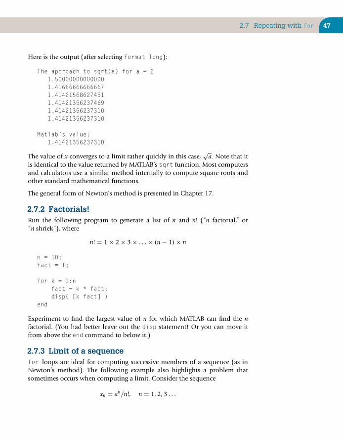
2.7 Repeating with for 47
Here is the output (after selecting format long):
The approach to sqrt(a) for a = 21.500000000000001.416666666666671.414215686274511.414213562374691.414213562373101.41421356237310
Matlab’s value:1.41421356237310
The value of x converges to a limit rather quickly in this case,√
a. Note that itis identical to the value returned by MATLAB’s sqrt function. Most computersand calculators use a similar method internally to compute square roots andother standard mathematical functions.
The general form of Newton’s method is presented in Chapter 17.
2.7.2 Factorials!Run the following program to generate a list of n and n! (“n factorial,” or“n shriek”), where
n! = 1 × 2 × 3 × . . . × (n − 1) × n
n = 10;fact = 1;
for k = 1:nfact = k * fact;disp( [k fact] )
end
Experiment to find the largest value of n for which MATLAB can find the nfactorial. (You had better leave out the disp statement! Or you can move itfrom above the end command to below it.)
2.7.3 Limit of a sequencefor loops are ideal for computing successive members of a sequence (as inNewton’s method). The following example also highlights a problem thatsometimes occurs when computing a limit. Consider the sequence
xn = an/n!, n = 1, 2, 3 . . .

48 CHAPTER 2: MATLAB Fundamentals
where a is any constant and n! is the factorial function defined above. Thequestion is this: What is the limit of this sequence as n gets indefinitely large?Let’s take the case a = 10. If we try to compute xn directly, we can get into trouble,because n! grows very rapidly as n increases, and numerical overflow can occur.However, the situation is neatly transformed if we spot that xn is related to xn−1
as follows:
xn = axn−1/n.
There are no numerical problems now.
The following program computes xn for a = 10 and increasing values of n.
a = 10;x = 1;k = 20; % number of terms
for n = 1:kx = a * x / n;disp( [n x] )
end
2.7.4 The basic for constructIn general the most common form of the for loop (for use in a program, noton the command line) is
for index = j:kstatements
end
or
for index = j:m:kstatements
end
Note the following points carefully:
■ j:k is a vector with elements j, j + 1, j + 2, . . . , k.
■ j:m:k is a vector with elements j, j + m, j + 2m, . . . , such that the lastelement does not exceed k if m > 0 or is not less than k if m < 0.
■ index must be a variable. Each time through the loop it will contain thenext element of the vector j:k or j:m:k, and statements (there may beone or more) are carried out for each of these values.
2.7 Repeating with for 49
If the for construct has the form
for k = first:increment:last
The number of times the loop is executed may be calculated from thefollowing equation:
floor
(last − first
increment
)+ 1
where the MATLAB function floor(x) rounds x down toward −∞. Thisvalue is called the iteration or trip count. As an example, let us considerthe statement for i = 1:2:6. It has an iteration count of
floor
(6 − 1
2
)+ 1 = floor
(52
)+ 1 = 3
Thus i takes the values 1, 3, 5. Note that if the iteration count isnegative, the loop is not executed.
■ On completion of the for loop the index contains the last value used.
■ If the vector j:k or j:m:k is empty, statements are not executed andcontrol passes to the statement following end.
■ The index does not have to appear explicitly in statements. It is basicallya counter. In fact, if the index does appear explicitly in statements, the forcan often be vectorized (more details on this are given in Section 2.7.7).A simple example of a more efficient (faster) program is as follows. Theexamples with disp at the beginning of this section were for illustrationonly; strictly, it would be more efficient to say (without “for”)
i = 1:5; disp( i’ )
Can you see the difference? In this case i is assigned as a vector (hence,this change vectorizes the original program).
■ It is good programming style to indent (tabulate) the statements inside afor loop. You may have noticed that the Editor does this for youautomatically with a feature called smart indenting. Indentingpreferences may be set from the Editor/Debugger’s File → Preferencesmenu. Expand the Editor/Debugger item in the Preferences menu andselect the Keyboard & Indenting Preferences dialogue box. Note alsothat a block of highlighted text may be (un)indented with the Editor’sText menu. You will also have noticed that the Editor implements syntaxhighlighting. Keywords are in one color, strings in another, and so on.You can customize the syntax-highlighting color scheme in theEditor/Debugger Font & Colors Preferences dialogue box. Click on SetColors in the Colors box (with Syntax highlighting checked).

50 CHAPTER 2: MATLAB Fundamentals
2.7.5 for in a single lineIf you insist on using for in a single line, here is the general form:
for index = j:k, statements, end
or
for index = j:m:k, statements, end
Note the following:
■ Don’t forget the commas (semicolons will also do if appropriate). If youleave them out you will get an error message.
■ Again, statements can be one or more statements separated by commasor semicolons.
■ If you leave out end, MATLAB will wait for you to enter it. Nothing willhappen until you do so.
2.7.6 More general forA more general form of for is
for index = v
where v is any vector. The index moves through each element of the vector inturn, providing a neat way of processing each item in a list. The most generalform of the for loop will be discussed in Chapter 6, when we look at matricesin more detail.
2.7.7 Avoid for loops by vectorizing!There are situations where a for loop is essential, as in many of the examplesin this section so far. However, given the way MATLAB has been designed, forloops tend to be inefficient in terms of computing time. If you have written afor loop that involves the index of the loop in an expression, it may be possibleto vectorize the expression, making use of array operations where necessary, asthe following examples show.
Suppose you want to evaluate1 00 000∑
n=1
n
(and can’t remember the formula for the sum). Here’s how to do it with a forloop (run the program, which also times how long it takes):
t0 = clock;

2.7 Repeating with for 51
s = 0;for n = 1:100000
s = s + n;endetime(clock, t0)
The MATLAB function clock returns a six-element vector with the current dateand time in the format year, month, day, hour, minute, seconds. Thus,t0 recordswhen the calculation starts.
The function etime returns the time in seconds elapsed between its two argu-ments, which must be vectors as returned by clock. On a Pentium II, it returnedabout 3.35 seconds, which is the total time for this calculation. (If you have afaster PC, it should take less time.)
Now try to vectorize this calculation (before looking at the solution). Here it is:
t0 = clock;n = 1:100000;s = sum( n );etime(clock, t0)
This way takes only 0.06 seconds on the same PC—more than 50 times faster!
There is a neater way of monitoring the time taken to interpret MATLABstatements: the tic and toc function. Suppose you want to evaluate
1 00 000∑n=1
1n2
Here’s the for loop version:
tics = 0;for n = 1:100000
s = s + 1/nˆ2;endtoc
which takes about 6 seconds on the same PC. Once again, try to vectorize thesum:
ticn = 1:100000;s = sum( 1./n.ˆ2 );toc

52 CHAPTER 2: MATLAB Fundamentals
The same PC gives a time of about 0.05 seconds for the vectorized version—more than 100 times faster! (Of course, the computation time in these examplesis small regardless of the method applied. However, learning how to improvethe efficiency of computation to solve more complex scientific or engineeringproblems will be helpful as you develop good programming skills. More detailson good problem-solving and program design practices are introduced at theend of this chapter and dealt with, in more detail, in the next.)
Series with alternating signs are a little more challenging. This series sums toln(2) (the natural logarithm of 2):
1 − 12
+ 13
− 14
+ 15
− · · ·
Here’s how to find the sum of the first 9999 terms with a for loop (note howto handle the alternating sign):
sign = –1;s = 0;for n = 1:9999sign = –sign;
s = s + sign / n;end
Try it. You should get 0.6932. MATLAB’s log(2) gives 0.6931. Not bad.
The vectorized version is as follows:
n = 1:2:9999;s = sum( 1./n – 1./(n+1) )
If you time the two versions, you will again find that the vectorized form ismany times faster.
MATLAB’s functions naturally exploit vectorization wherever possible. Forexample, prod(1:n) will find n! much faster than the code at the beginning ofthis section (for large values of n).
EXERCISES
Write MATLAB programs to find the following sums with for loops and by vectorization. Timeboth versions in each case.
■ 12 + 22 + 32 + · · · + 1 0002 (sum is 333 833 500)
■ 1 − 13
+ 15
− 17
+ 19
− · · · − 11003
(sum is 0.7849—converges slowly to π/4)

2.8 Decisions 53
■ Sum the left-hand side of the series
112 · 32
+ 132 · 52
+ 152 · 72
+ · · · = π2 − 816
(sum is 0.1169—with 500 terms)
2.8 DECISIONS
The MATLAB function rand generates a random number in the range 0–1. Enterthe following two statements at the command line:
r = randif r > 0.5 disp( ’greater indeed’ ), end
MATLAB should only display the message greater indeed if r is in fact greaterthan 0.5 (check by displaying r). Repeat a few times—cut and paste from theCommand History window (make sure that a new r is generated each time).
As a slightly different but related exercise, enter the following logical expressionon the command line:
2 > 0
Now enter the logical expression –1 > 0. MATLAB gives a value of 1 to a logicalexpression that is true and 0 to one that is false.
2.8.1 The one-line if statementIn the last example MATLAB has to make a decision; it must decide whetheror not r is greater than 0.5. The if construct, which is fundamental to allcomputing languages, is the basis of such decision making. The simplest formof if in a single line is
if condition statement, end
Note the following points:
■ condition is usually a logical expression (i.e., it contains a relationaloperator), which is either true or false. The relational operators are shownin Table 2.4. MATLAB allows you to use an arithmetic expression forcondition. If the expression evaluates to 0, it is regarded as false; anyother value is true. This is not generally recommended; the if statementis easier to understand (for you or a reader of your code) if condition is alogical expression.
■ If condition is true, statement is executed, but if condition is false, nothinghappens.

54 CHAPTER 2: MATLAB Fundamentals
Table 2.4 Relational Operators
Operator Meaning
< Less than<= Less than or equal== Equal∼= Not equal to> Greater than>= Greater than or equal
■ condition may be a vector or a matrix, in which case it is true only if all ofits elements are nonzero. A single zero element in a vector or matrixrenders it false.
Here are more examples of logical expressions involving relational operators,with their meanings in parentheses:
b∧2 < 4*a*c (b2 < 4ac)x >= 0 (x ≥ 0)a ∼= 0 (a �= 0)b∧2 == 4*a*c (b2= 4ac)
Remember to use the double equal sign (==) when testing for equality:
if x == 0 disp( ’x equals zero’), end
EXERCISES
The following statements all assign logical expressions to the variable x. See if you can correctlydetermine the value of x in each case before checking your answer with MATLAB.
(a) x = 3 > 2(b) x = 2 > 3(c) x = –4 <= –3(d) x = 1 < 1(e) x = 2 ∼= 2(f) x = 3 == 3(g) x = 0 < 0.5 < 1
Did you get (f)? 3 == 3 is a logical expression that is true since 3 is undoubtedly equal to 3.The value 1 (for true) is therefore assigned to x.What about (g)? As a mathematical inequality,
0 < 0.5 < 1

2.8 Decisions 55
is undoubtedly true from a nonoperational point of view. However, as a MATLAB operationalexpression, the left-hand < is evaluated first, 0 < 0.5, giving 1 (true). Then the right-handoperation is performed, 1 < 1, giving 0 (false). Makes you think, doesn’t it?
2.8.2 The if-else constructIf you enter the two lines
x = 2;if x < 0 disp( ’neg’ ), else disp( ’non-neg’), end
do you get the message non-neg? If you change the value of x to −1 and executethe if again, do you get the message neg this time? Finally, if you try
if 79 disp( ’true’ ), else disp(’false’ ), end
do you get true? Try other values, including 0 and some negative values.
Most banks offer differential interest rates. Suppose the rate is 9% if the amountin your savings account is less than $5000, but 12% otherwise. The RandomBank goes one step further and gives you a random amount in your account tostart with! Run the following program a few times:
bal = 10000 * rand;
if bal < 5000rate = 0.09;
elserate = 0.12;
end
newbal = bal + rate * bal;disp( ’New balance after interest compounded is:’ )format bankdisp( newbal )
Display the values of bal and rate each time from the command line to checkthat MATLAB has chosen the correct interest rate.
The basic form of if-else for use in a program file is
if conditionstatementsA
elsestatementsB
end

56 CHAPTER 2: MATLAB Fundamentals
Note that
■ statementsA and statementsB represent one or more statements.
■ If condition is true, statementsA are executed, but if condition is false,statementsB are executed. This is essentially how you force MATLAB tochoose between two alternatives.
■ else is optional.
2.8.3 The one-line if-else statementThe simplest general form of if-else for use on one line is
if condition statementA, else statementB, end
Note the following:
■ Commas (or semicolons) are essential between the various clauses.
■ else is optional.
■ end is mandatory; without it, MATLAB will wait forever.
2.8.4 elseifSuppose the Random Bank now offers 9% interest on balances of less than$5000, 12% for balances of $5000 or more but less than $10,000, and 15% forbalances of $10,000 or more. The following program calculates a customer’snew balance after one year according to this scheme:
bal = 15000 * rand;
if bal < 5000rate = 0.09;
elseif bal < 10000rate = 0.12;
elserate = 0.15;
end
newbal = bal + rate * bal;format bankdisp( ’New balance is:’ )disp( newbal )

2.8 Decisions 57
Run the program a few times, and once again display the values of bal and rateeach time to convince yourself that MATLAB has chosen the correct interest rate.
In general, the elseif clause is used:
if condition1statementsA
elseif condition2statementsB
elseif condition3statementsC
...else
statementsEend
This is sometimes called an elseif ladder. It works as follows:
1. condition1 is tested. If it is true, statementsA are executed; MATLAB thenmoves to the next statement after end.
2. If condition1 is false, MATLAB checks condition2. If it is true, statementsBare executed, followed by the statement after end.
3. In this way, all conditions are tested until a true one is found. As soon asa true condition is found, no further elseifs are examined and MATLABjumps off the ladder.
4. If none of the conditions is true, statementsE after else are executed.
5. Arrange the logic so that not more than one of the conditions is true.
6. There can be any number of elseifs, but at most one else.
7. elseif must be written as one word.
8. It is good programming style to indent each group of statements asshown.
2.8.5 Logical operatorsMore complicated logical expressions can be constructed using the three logicaloperators: & (and), | (or), and ˜ (not). For example, the quadratic equation
ax2 + bx + c = 0

58 CHAPTER 2: MATLAB Fundamentals
00
0.5 1 1.5 2 2.5 3 3.5 4
0.5
1
1.5
2
2.5
3
3.5
4
FIGURE 2.2Quadratic function with equal roots.
has equal roots, given by −b/(2a), provided that b2 − 4ac = 0 and a �= 0(Figure 2.2). This translates into the following MATLAB statements:
if (b ˆ 2 – 4*a*c == 0) & (a ∼= 0)x = –b / (2*a);
end
Of course, a, b, and c must be assigned values prior to reaching this set ofstatements. Note the double equal sign in the test for equality; see Chapter 5for more on logical operators.
2.8.6 Multiple ifs versus elseifYou could have written the Random Bank program as follows:
bal = 15000 * rand;
if bal < 5000rate = 0.09;
endif bal >= 5000 & bal < 10000
rate = 0.12;endif bal >= 10000
rate = 0.15;end

2.8 Decisions 59
newbal = bal + rate * bal;format bankdisp( ’New balance is’ )disp( newbal )
However, this is inefficient since each of the three conditions is always tested,even if the first one is true. In the earlier elseif version, MATLAB jumps off theelseif ladder as soon as it finds a true condition. This saves a lot of computingtime (and is easier to read) if the if construct is in a loop that is repeated often.
Using this form, instead of the elseif ladder, you can make the followingcommon mistake:
if bal < 5000rate = 0.09;
endif bal < 10000
rate = 0.12;endif bal >= 10000
rate = 0.15;end
Can you see why you get the wrong answer (1120 instead of 1090) if bal hasthe value 1000? When designing the logic, you need to make sure that one andonly one of the conditions will be true at any one time.
Another mistake frequently made is to replace the second if with somethinglike
if 5000 < bal < 10000rate = 0.12;
end
which is compelling, as we saw above. However, whatever the value of bal, thiscondition will always be true. Can you see why? (Note that if bal is greater than5000—for example, bal = 20000—the numerical truth value of the first test,namely, 5000 < bal, is true and hence has the numerical value of 1 since 1 isalways less than 10000, even if bal = 20000.)
2.8.7 Nested ifsAn if construct can contain further ifs and so on. This is called nesting andshould not be confused with the elseif ladder. You have to be careful withelses. In general, else belongs to the most recent if that has not been ended.The correct positioning of end is therefore very important, as the next exampledemonstrates.

60 CHAPTER 2: MATLAB Fundamentals
Suppose you want to compute the solution to a quadratic equation. You maywant to check whether a = 0 to prevent a division by zero. Your program couldcontain the following nested ifs:
...d = bˆ 2 – 4*a*c;if a ∼= 0if d < 0disp( ’Complex roots’ )
elsex1 = (–b + sqrt( d )) / (2*a);x2 = (–b – sqrt( d )) / (2*a);
end % first end ««««««end
The else belongs to the second if by default, as intended.
Now move the first end up as follows:
d = bˆ 2 – 4*a*c;if a ∼= 0if d < 0disp( ’Complex roots’ )
end % first end moved up now ««««««elsex1 = (–b + sqrt( d )) / (2*a);x2 = (–b – sqrt( d )) / (2*a);
end
The end that has been moved now closes the second if. The result is that elsebelongs to the first if instead of to the second one. Division by zero is thereforeguaranteed instead of prevented!
2.8.8 Vectorizing ifs?You may be wondering if for statements enclosing ifs can be vectorized. Theanswer is yes, courtesy of logical arrays. Discussion of this rather interesting topicis postponed until Chapter 5.
2.8.9 The switch statementswitch executes certain statements based on the value of a variable or expres-sion. In this example it is used to decide whether a random integer is 1, 2, or 3(see Section 5.1.5 for an explanation of this use of rand):
d = floor(3*rand) + 1switch d

2.9 Complex Numbers 61
case 1disp( ’That’’s a 1!’ );
case 2disp( ’That’’s a 2!’ );
otherwisedisp( ’Must be 3!’ );
end
Multiple expressions can be handled in a single case statement by enclosingthe case expression in a cell array (see Chapter 11):
d = floor(10*rand);switch dcase {2, 4, 6, 8}
disp( ’Even’ );case {1, 3, 5, 7, 9}
disp( ’Odd’ );otherwise
disp( ’Zero’ );end
2.9 COMPLEX NUMBERS
If you are not familiar with complex numbers, you can safely skip this section.However, it is useful to know what they are since the square root of a negativenumber may come up as a mistake if you are trying to work only with realnumbers.
It is very easy to handle complex numbers in MATLAB. The special values iand j stand for
√−1. Try sqrt(–1) to see how MATLAB represents complexnumbers.
The symbol i may be used to assign complex values, for example,
z = 2 + 3*i
represents the complex number 2 + 3i (real part 2, imaginary part 3). You canalso input a complex value like this:
2 + 3*i
in response to the input prompt (remember, no semicolon). The imaginarypart of a complex number may also be entered without an asterisk, 3i.
All of the arithmetic operators (and most functions) work with complex num-bers, such as sqrt(2 + 3*i) and exp(i*pi). Some functions are specific to

62 CHAPTER 2: MATLAB Fundamentals
complex numbers. If z is a complex number, real(z), imag(z), conj(z), andabs(z) all have the obvious meanings.
A complex number may be represented in polar coordinates:
z = reiθ
angle(z) returns θ between −π and π; that is, atan2(imag(z), real(z)).abs(z) returns the magnitude r.
Since eiθ gives the unit circle in polars, complex numbers provide a neat way ofplotting a circle. Try the following:
circle = exp( 2*i*[1:360]*pi/360 );plot(circle)axis(’equal’)
Note these points:
■ If y is complex, the statement plot(y) is equivalent to
plot(real(y), imag(y))
■ The statement axis(’equal’) is necessary to make circles lookround; it changes what is known as the aspect ratio of the monitor.axis(’normal’) gives the default aspect ratio.
If you are using complex numbers, be careful not to use i or j for othervariables; the new values will replace the value of
√−1 and will cause nastyproblems.
For complex matrices, the operations ’ and .’ behave differently. The ’operator is the complex conjugate transpose, meaning rows and columns are inter-changed and signs of imaginary parts are changed. The .’ operator, on the otherhand, does a pure transpose without taking the complex conjugate. To see this,set up a complex matrix a with the statement
a = [1+i 2+2i; 3+3i 4+4i]
which results in
a =1.0000 + 1.0000i 2.0000 + 2.0000i3.0000 + 3.0000i 4.0000 + 4.0000i
The statement
a’

2.10 More on Input and Output 63
then results in the complex conjugate transpose
ans =1.0000 – 1.0000i 3.0000 – 3.0000i2.0000 – 2.0000i 4.0000 – 4.0000i
whereas the statement
a.’
results in the pure transpose
ans =1.0000 + 1.0000i 3.0000 + 3.0000i2.0000 + 2.0000i 4.0000 + 4.0000i
2.10 MORE ON INPUT AND OUTPUT
This section is not “essential” MATLAB; you can skip it and come back at a latertime.
2.10.1 fprintfTo control exactly what your output looks like, you should use the fprintffunction. Otherwise, you can stay with disp, format, and cut and paste.
The fprintf statement is much more flexible (and therefore more compli-cated!) than disp. For example, it allows you to mix strings and numbers freelyon the same line and to completely control formatting (e.g., number of decimalplaces). As an example, change your compound interest program (Section 1.3.2)as follows:
balance = 12345;rate = 0.09;interest = rate * balance;balance = balance + interest;fprintf( ’Interest rate: %6.3f New balance: %8.2f\n’, ...
rate, balance );
Your output should look like this:
Interest rate: 0.090 New balance: 13456.05
The most common form of fprintf is
fprintf( ’format string’, list of variables )

64 CHAPTER 2: MATLAB Fundamentals
Note the following:
■ format string may contain a message. It may also contain format specifiersof the form %e, %f, or %g, which control how the variables listed areembedded in the format string.
■ In the case of the e and f specifiers, the field width and number ofdecimal places or significant digits may be specified immediately afterthe %, as the next two examples show.
■ %8.3f means fixed-point over 8 columns altogether (including thedecimal point and a possible minus sign), with 3 decimal places(spaces are filled in from the left if necessary). Use 0 if you don’t wantany decimal places, e.g., %6.0f. Use leading zeros if you want leadingzeros in the output, e.g., %03.0f.
■ %12.2e means scientific notation over 12 columns altogether(including the decimal point, a possible minus sign, and five for theexponent), with 2 digits in the mantissa after the decimal point (themantissa is always adjusted to be not less than 1).
■ The g specifier is mixed and leaves it up to MATLAB to decide exactlywhat format to use. This is a good one to use if you can’t be bothered tocount decimal places carefully and/or aren’t sure of the approximatemagnitude of your result.
■ In the case of a vector, the sequence of format specifiers is repeated untilall the elements have been displayed.
■ The format string in fprintf may also contain escape codes such as \n(line feed), \t (horizontal tab), \b (backspace), and \f (form feed).
A C programmer will no doubt feel very much at home here! For more details,see fprintf in the online Help.
2.10.2 Output to a disk file with fprintfOutput may be sent to a disk file with fprintf. The output is appended, that is,added to the end of the file.
The general form is
fprintf( ’filename’, ’format string’, list of variables )
For example,
fprintf( ’myfile’, ’%g’, x )
sends the value of x to the disk file myfile.
2.11 Odds and Ends 65
2.10.3 General file I/OMATLAB has a useful set of file I/O functions, such as fopen, fread, fwrite,and fseek, which are discussed in Chapter 4.
2.10.4 Saving and loading dataAll or part of the workspace can be saved to a disk file and reloaded in a latersession with the save and load commands. See Chapter 4 for details on theseand other ways of importing and exporting MATLAB data.
2.11 ODDS AND ENDS
In this section we deal with additional information on naming variablesand functions. We also introduce the input function, shelling out and helpfunctions.
2.11.1 Variables, functions, and scripts with the samename
Enter the command rand. You will get a random number—in fact, a differentone—each time. Now enter the statement
rand = 13;
randnow represents a variable with the value 13 (check withwhos). The randomnumber generator rand has been hidden by the variable of the same name andis unavailable until you clear rand. A script file can also be hidden like this.
When you type a name at the command-line prompt, say goo, the MATLABinterpreter goes through the following steps:
1. Looks for goo as a variable.
2. Looks in the Current Directory for a script file called goo.m.
3. Looks for goo as a built-in function, such as sin or pi.
4. Looks (in order) in the directories specified by MATLAB’s search pathfor a script file called goo.m. (You may use File → Set Path to view andchange MATLAB’s search path.)
I have seen students accidentally hiding scripts in this way during hands-ontests—it is a traumatic experience. If you are worried that there might be aMATLAB function goo lurking around to hide your script of the same name,first try help goo. If you get the message goo.m not found, then you’re safe.To unhide a hidden goo, type clear goo.

66 CHAPTER 2: MATLAB Fundamentals
2.11.2 The input statementCarefully rewrite the script file compint.m so that it looks exactly like this(remember to save it):
balance = input( ’Enter bank balance: ’ );rate = input( ’Enter interest rate: ’ );interest = rate * balance;balance = balance + interest;format bankdisp( ’New balance:’ );disp( balance );
Enter the script file name at the prompt and, when asked, enter values of 1000and 0.15 for the balance and interest rate, respectively, so that your CommandWindow contains the following lines:
�compint
Enter bank balance: 1000
Enter interest rate: 0.15New balance:
1150.00
The input statement provides a more flexible way of getting data into a programthan by assignment statements, which need to be edited each time the data mustbe changed. It allows you to enter data while a script is running. The general formof the input statement is
variable = input(’ prompt’);
Note that
■ The prompt message prompts for the value(s) to be entered. It must beenclosed in apostrophes (single quotes).
■ A semicolon at the end of the input statement will prevent the valueentered from being immediately echoed on the screen.
■ You normally do not use input from the command line, since youshouldn’t need to prompt yourself in command-line mode.
■ Vectors and matrices may also be entered with input, as long as youremember to enclose the elements in square brackets.
■ You can enter an expression in response to the prompt—for example,a + b (as long as a and b have been defined) or rand(5). When

2.12 Programming Style 67
entering an expression in this way, don’t include a semicolon (it is notpart of the expression).
EXERCISES
2.1. Rewrite the solutions to a few of the unit conversion problems in Section 2.5 usinginput statements in script files.
2.2. Rewrite the program comp.m in Section 2.5.11 to input the initial investment vector.
2.11.3 Shelling out to the operating systemYou can shell out of MATLAB to the operating system by prefacing an operatingsystem command with an exclamation point (bang). For example, suppose yousuddenly need to reset the system time during a MATLAB session. You can dothis from the Command Window with the command
!time
(under Windows). Shelling out is achieved without quitting the currentMATLAB session.
2.11.4 More Help functionsBy now you should be finding your way around MATLAB’s online Help. Hereare some alternative command-line ways of getting help. The command docfunction displays the reference page for function in the Help browser, providingsyntax, a description, examples, and links to related functions. The commandhelpwin displays a list of all functions in the Help browser, with links to M-fileHelp for each one.
2.12 PROGRAMMING STYLE
Some programmers delight in writing terse and obscure code; there is at leastone annual competition for the most incomprehensible C program. Manyresponsible programmers, however, believe it is extremely important to developthe art of writing programs that are well laid out, with all the logic clearlydescribed. They therefore pay a fair amount of attention to what is calledprogramming style to make their programs clearer and more readable both tothemselves and to users. You may find this irritating if you are starting to pro-gram for the first time, because you will naturally be impatient to get on with thejob. However, a little extra attention to your program layout will pay enormousdividends in the long run, especially when it comes to debugging.

68 CHAPTER 2: MATLAB Fundamentals
Here are some hints on how to improve your programming style:
■ You should make liberal use of comments, both at the beginning of ascript to describe briefly what it does and any special methods that mayhave been used, and throughout the coding to introduce differentlogical sections.
■ The meaning of each variable should be described briefly in a commentwhen it is initialized. You should describe variables systematically, forexample, in alphabetical order.
■ Blank lines should be freely used to separate sections of coding (e.g.,before and after loop structures).
■ Coding (i.e., statements) inside structures (fors, ifs, whiles) should beindented (tabulated) a few columns to make them stand out.
■ Blank spaces should be used in expressions to make them morereadable—for example, on either side of operators and equal signs.However, blanks may be omitted in places in complicated expressionswhere this may make the logic clearer.
The development of the problem statement is, probably, the most difficult partof any design process; it is no different for the design of a program. Hence,learning to design good programs (or codes, as they are sometimes called)provides good experience in the practice of creative design. A strategic planis required that leads to the development of an algorithm (i.e., the sequenceof operations required for solving a problem in a finite number of steps) forMATLAB to execute in order to provide an answer to the problem posed. Theessential goal is to create a top-down structure plan itemizing all of the steps ofthe algorithm to obtain the desired solution. The methodology of developingsuch a plan is described in more detail in the next chapter.
SUMMARY
■ The MATLAB desktop consists of a number of tools: the CommandWindow, the Workspace browser, the Current Directory browser, and theCommand History window.
■ MATLAB has a comprehensive online Help system. It can be accessedthrough the Help button (?) on the desktop toolbar or the Help menu inany tool.
■ A MATLAB program can be written in the Editor and cut and pasted to theCommand Window (or it can be executed from the editor by clicking thegreen right arrow in the toolbar at the top of the Editor window).

Summary 69
■ A script file is a text file (created by the MATLAB Editor or any other texteditor) containing a collection of MATLAB statements. In other words, it is aprogram. The statements are carried out when the script file name is enteredat the prompt in the Command Window. A script file name must have the.m extension. Script files are therefore also called M-files.
■ The recommended way to run a script is from the Current Directory browser.The output from the script will then appear in the Command Window.
■ A variable name consists only of letters, digits, and underscores, and muststart with a letter. Only the first 63 characters are significant. MATLAB iscase-sensistive by default. All variables created during a session remain inthe workspace until removed with clear. The command who lists thevariables in the workspace; whos gives their sizes.
■ MATLAB refers to all variables as arrays, whether they are scalars(single-valued arrays), vectors, (1D arrays), or matrices (2D arrays).
■ MATLAB names are case-sensitive.
■ The Workspace browser on the desktop provides a handy visualrepresentation of the workspace. Clicking a variable in it invokes the ArrayEditor, which may be used to view and change variable values.
■ Vectors and matrices are entered in square brackets. Elements are separatedby spaces or commas. Rows are separated by semicolons. The colonoperator is used to generate vectors, with elements increasing (decreasing)by regular increments (decrements). Vectors are row vectors by default. Usethe apostrophe transpose operator (’) to change a row vector into a columnvector.
■ An element of a vector is referred to by a subscript in parentheses.A subscript may itself be a vector. Subscripts always start at 1.
■ The diary command copies everything that subsequently appears in theCommand Window to the specified text file until the command diary offis given.
■ Statements on the same line may be separated by commas or semicolons.
■ A statement may be continued to the next line with an ellipsis of at leastthree dots.
■ Numbers may be represented in fixed-point decimal notation or infloating-point scientific notation.
■ MATLAB has 14 data types. The default numeric type is double precision.All mathematical operations are carried out in double precision.

70 CHAPTER 2: MATLAB Fundamentals
■ The six arithmetic operators for scalars are +, –, *, \, /, and ˆ. Theyoperate according to rules of precedence.
■ An expression is a rule for evaluating a formula using numbers, operators,variables, and functions. A semicolon after an expression suppresses displayof its value.
■ Array operations are element by element between vectors or between scalarsand vectors. The array operations of multiplication, right and left division,and exponentiation are indicated by .*, ./, .\, and .ˆ todistinguish them from vector and matrix operations of the same name.They may be used to evaluate a formula repeatedly for some or all of theelements of a vector. This is called vectorization of the formula.
■ disp is used to output (display) numbers and strings. num2str is usefulwith disp for displaying strings and numbers on the same line.
■ The format command controls the way output is displayed. Format mayalso be set by File → Preferences → Command Window Preferences.
■ When vectors are displayed, a common scale factor is used if the elementsare very large or very small, or differ greatly in magnitude.
■ The for statement is used to repeat a group of statements a fixed number oftimes. If the index of a for statement is used in the expression beingrepeated, the expression can often be vectorized, saving a great deal ofcomputing time.
■ tic and toc may be used as a stopwatch.
■ Logical expressions have the value true (1) or false (0) and are constructedwith the six relational operators >, >=, <, <=, ==, and ˜=. Anyexpression that evaluates to zero is regarded as false. Any other value is true.More complicated logical expressions can be formed from other logicalexpressions using the logical operators & (and), | (or), and ˜ (not).
■ if–else executes different groups of statements according to whether alogical expression is true or false. The elseif ladder is a good way to choosebetween a number of options, only one of which should be true at a time.
■ switch enables choices to be made between discrete cases of a variable orexpression.
■ A string is a collection of characters enclosed in apostrophes.
■ Complex numbers may be represented using the special variables i and j,which stand for the unit imaginary number
√−1.
■ fprintf is used to precisely control output format.

Summary 71
■ save and load are used to export and import data.
■ The input statement, with a prompt, is used to prompt for input from thekeyboard while a script is executing.
■ MATLAB checks whether a name is a variable, then a built-in function, thena script. Use clear to unhide a function or script if necessary.
■ Operating system commands can be executed from the MATLAB prompt bytyping an exclamation point in front of them (e.g., !copy). This is calledshelling out.
■ Attention should be paid to programming style when writing scripts.
CHAPTER EXERCISES
2.1. Decide which of the following numbers are not acceptable in MATLAB, and statewhy:(a) 9,87
(b) .0
(c) 25.82
(d) –356231
(e) 3.57*e2
(f) 3.57e2.1
(g) 3.57e+2
(h) 3,57e–2
2.2. State, giving reasons, which of the following are not valid MATLAB variable names:(a) a2
(b) a.2
(c) 2a
(d) ’a’one
(e) aone
(f) _x_1
(g) miXedUp
(h) pay day
(i) inf
(j) Pay_Day
(k) min*2
(l) what
(Continued)
2.3. Translate the following expressions into MATLAB:
(a) p + wu

72 CHAPTER 2: MATLAB Fundamentals
(b) p + wu + v
(c)p + w
u+v
p + wu−v
(d) x 1/2
(e) y y+z
(f) x y z
(g) (x y )z
(h) x − x 3/3! + x 5/5!2.4. Translate the following into MATLAB statements:
(a) Add 1 to the value of i and store the result in i.
(b) Cube i, add j to this, and store the result in i.
(c) Set g equal to the larger of the two variables e and f.
(d) If d is greater than 0, set x equal to −b.
(e) Divide the sum of a and b by the product of c and d, and store the result in x.
2.5. What’s wrong with the following MATLAB statements?(a) n + 1 = n;
(b) Fahrenheit temp = 9*C/5 + 32;
(c) 2 = x;
2.6. Write a program to calculate x , where
x = −b +√
b2 − 4ac2a
and a = 2, b = −10, c = 12 (Answer 3.0)
2.7. There are eight pints in a gallon and 1.76 pints in a liter. The volume of a tank is givenas 2 gallons and 4 pints. Write a script that inputs this volume in gallons and pints andconverts it to liters. (Answer: 11.36)
2.8. Write a program to calculate gasoline consumption. It should assign the distance trav-eled (in kilometers) and the amount of gas used (in liters) and compute the consumptionin km/liter as well as in the more usual form of liters/100 km. Write some helpfulheadings so that your output looks something like this:
Distance Liters used km/L L/100km
528 46.23 11.42 8.76
2.9. Write some statements in MATLAB that exchange the contents of two variablesa andb, using only one additional variable t.
2.10. Try Exercise 2.9 without using any additional variables!
2.11. If C and F are Celsius and Fahrenheit temperatures, respectively, the formula forconversion from Celsius to Fahrenheit is F = 9C/5 + 32.(a) Write a script that will ask you for the Celsius temperature and display the
Fahrenheit equivalent with some sort of comment, such as
The Fahrenheit temperature is:...

Summary 73
Try it out on the following Celsius temperatures (answers in parentheses):0 (32), 100 (212), −40 (−40!), 37 (normal human temperature: 98.6).
(b) Change the script to use vectors and array operations to compute the Fahrenheitequivalents of Celsius temperatures ranging from 20◦ to 30◦ in steps of 1◦, anddisplay them in two columns with a heading, like this:
Celsius Fahrenheit20.00 68.0021.00 69.80...30.00 86.00
2.12. Generate a table of conversions from degrees (first column) to radians (second column).Degrees should go from 0◦ to 360◦ in steps of 10◦. Recall that π radians = 180◦.
2.13. Set up a matrix (table) with degrees in the first column from 0 to 360 in steps of 30,sines in the second column, and cosines in the third column. Now try to add tangentsin the fourth column. Can you figure out what’s going on? Try some variations of theformat command.
2.14. Write some statements that display a list of integers from 10 to 20 inclusive, each withits square root next to it.
2.15. Write a single statement to find and display the sum of the successive even integers2, 4,… , 200. (Answer: 10,100)
2.16. Ten students in a class take a test. The marks are out of 10. All the marks are enteredin a MATLAB vector, marks. Write a statement to find and display the average mark.Try it on the following:
5 8 0 10 3 8 5 7 9 4 (Answer: 5.9)
Hint : use the mean function.
2.17. What are the values of x and a after the following statements have been executed?
(a) a = 0;
(b) i = 1;
(c) x = 0;
(d) a = a + i;
(e) x = x + i / a;
(f) a = a + i;
(g) x = x + i / a;
(h) a = a + i;
(i) x = x + i / a;
(j) a = a + i;
(k) x = x + i / a;
(Continued)
2.18. Rewrite the statements in Exercise 2.17 more economically by using a for loop. Canyou do even better by vectorizing the code?

74 CHAPTER 2: MATLAB Fundamentals
2.19. Work out by hand the output of the following script for n = 4:
n = input( ’Number of terms? ’ );s = 0;
for k = 1:ns = s + 1 / (k ˆ 2);
end;
disp(sqrt(6 * s))
If you run this script for larger and larger values of n, you will find that the outputapproaches a well-known limit. Can you figure out what it is? Now rewrite the scriptusing vectors and array operations.
2.20. Work through the following script by hand. Draw up a table of the values of i,j, and mto show how they change while the script executes. Check your answers by runningthe script.
v = [3 1 5];i = 1;
for j = vi = i + 1;if i == 3
i = i + 2;m = i + j;
endend
2.21. The steady-state current I flowing in a circuit that contains a resistance R = 5,capacitance C = 10, and inductance L = 4 in series is given by
I = E√R2 + (
2πωL − 12πωC
)2
where E = 2 and ω = 2 are the input voltage and angular frequency, respectively.Compute the value of I . (Answer: 0.0396)
2.22. The electricity accounts of residents in a very small town are calculated as follows:
■ If 500 units or fewer are used, the cost is 2 cents per unit.■ If more than 500 but not more than 1000 units are used, the cost is $10 for the
first 500 units and 5 cents for every unit in excess of 500.■ If more than 1000 units are used, the cost is $35 for the first 1000 units plus 10
cents for every unit in excess of 1000.■ A basic service fee of $5 is charged, no matter how much electricity is used.
Write a program that enters the following five consumptions into a vector and uses afor loop to calculate and display the total charge for each one: 200, 500, 700, 1000,1500. (Answers: $9, $15, $25, $40, $90)

Summary 75
2.23. Suppose you deposit $50 in a bank account every month for a year. Every month, afterthe deposit has been made, interest at the rate of 1% is added to the balance: Afterone month the balance is $50.50, and after two months it is $101.51. Write a programto compute and print the balance each month for a year. Arrange the output to looksomething like this:
MONTH MONTH-END BALANCE
1 50.502 101.513 153.02...12 640.47
2.24. If you invest $1000 for one year at an interest rate of 12%, the return is $1120 at the endof the year. But if interest is compounded at the rate of 1% monthly (i.e., 1/12 of theannual rate), you get slightly more interest because it is compounded. Write a programthat uses a for loop to compute the balance after a year of compounding interest inthis way.The answer should be $1126.83. Evaluate the formula for this result separatelyas a check: 1000 × 1.0112.
2.25. A plumber opens a savings account with $100,000 at the beginning of January. He thenmakes a deposit of $1000 at the end of each month for the next 12 months (starting atthe end of January). Interest is calculated and added to his account at the end of eachmonth (before the $1000 deposit is made). The monthly interest rate depends on theamount A in his account at the time interest is calculated, in the following way:
A ≤ 1 10 000 : 1%1 10 000 < A ≤ 1 25 000 : 1.5%
A > 1 25 000 : 2%
Write a program that displays, under suitable headings, for each of the 12 months, thesituation at the end of the month as follows: the number of the month, the interest rate,the amount of interest, and the new balance. (Answer:Values in the last row of outputshould be 12, 0.02, 2534.58, 130263.78).
2.26. It has been suggested that the population of the United States may be modeled by theformula
P (t) = 19 72 73 0001 + e−0.03134(t−1913.25)
where t is the date in years. Write a program to compute and display the populationevery ten years from 1790 to 2000. Try to plot a graph of the population against time aswell (Figure 7.14 shows this graph compared with actual data). Use your program tofind out if the population ever reaches a “steady state” (i.e., stops changing).
(Continued)
2.27. A mortgage bond (loan) of amount L is obtained to buy a house. The interest rate r is15%.The fixed monthly payment P that will pay off the bond loan over N years is givenby the formula
P = rL(1 + r/12)12N
12[(1 + r/12)12N − 1]

76 CHAPTER 2: MATLAB Fundamentals
(a) Write a program to compute and print P if N = 20 and the bond is for $50,000.You should get $658.39.
(b) See how P changes with N by running the program for different values of N(use input). Can you find a value for which the payment is less than $625?
(c) Go back to N = 20 and examine the effect of different interest rates.You shouldsee that raising the interest rate by 1% (0.01) increases the monthly paymentby about $37.
2.28. It is useful to work out how the period of a bond repayment changes if you increase ordecrease P . The formula for N is given by
N =ln
(P
P−rL/12
)12 ln(1 + r/12)
(a) Write a new program to compute this formula. Use the built-in function logfor the natural logarithm ln. How long will it take to pay off a loan of $50,000 at$800 a month if the interest remains at 15%? (Answer: 10.2 years—nearly twiceas fast as when paying $658 a month.)
(b) Use your program to find out by trial and error the smallest monthly paymentthat will pay off the loan this side of eternity. Hint : recall that it is not possibleto find the logarithm of a negative number, so P must not be less than rL/12.

CHAPTER 3
Program Design and Algorithm Development
The objectives of this chapter are to introduce you to
■ Program design■ The structure plan (pseudo-code) as a means of designing the logic of
a program
This chapter is an introduction to the design of computer programs. Thetop-down design process is elaborated to help you think about good problem-solving strategies as they relate to the design of procedures for using softwarelike MATLAB. We will consider the design of your own toolbox to be includedamong those already available with your version of MATLAB, such as Simulink,Symbolic Math, and Controls System. This is a big advantage of MATLAB (andtools like it); it allows you to customize your working environment to meetyour own needs. It is not only the “mathematics handbook” of today’s stu-dent, engineer, and scientist, it is also a useful environment to develop softwaretools that go beyond any handbook to help you to solve relatively complicatedmathematical problems.
In the first part of this chapter we discuss the design process. In the second partwe examine the structure plan—the detailed description of the algorithm to beimplemented. We will consider relatively simple programs. However, the pro-cess described is intended to provide insight into what you will confront whenyou deal with more complex engineering, scientific, and mathematical prob-lems during the later years of your formal education, your life-long learning,and your continuing professional education.
To be sure, the examples examined so far have been logically simple. This isbecause we have been concentrating on the technical aspects of writing correctCopyright © 2010, Daniel T. Valentine. Published by Elsevier Ltd. All rights reserved.DOI: 10.1016/B978-0-12-374883-6.00003-5 77

78 CHAPTER 3: Program Design and Algorithm Development
MATLAB statements. It is very important to learn how MATLAB does the arith-metic operations that form the basis of more complex programs. To design asuccessful program you need to understand a problem thoroughly and breakit down into its most fundamental logical stages. In other words, you have todevelop a systematic procedure or algorithm for solving it.
There are a number of methods that may assist in algorithm development. Inthis chapter we look at one, the structure plan. You briefly met the concept ofa structure plan. Its development is the primary part of the software (or code)design process because it is the steps in it that are translated into a languagethe computer can understand—for example, into MATLAB commands, someof which were introduced in the previous two chapters.
3.1 THE PROGRAM DESIGN PROCESS
Useful utilities translated into MATLAB (either sequences of command lines orfunctions, which are described later in the text) and saved as M-files in your work-ing directory are your primary goals. There are numerous toolboxes availablethrough MathWorks (among others) on a variety of engineering and scientifictopics. A great example is the Aerospace Toolbox, which provides referencestandards, environmental models, and aerodynamic coefficient importing foradvanced aerospace engineering designs. Explore the MathWorks Web site forproducts available (http://www.mathworks.com/).
In the default working directory, \work, or in your own working directory (e.g.,\mytools), you will begin to accumulate a set of M-files that you have createdas you use MATLAB. One way to create and to get to your own working directoryis to execute the following commands:
� mkdir mytools <Enter>� cd mytools <Enter>
Certainly, you want to be sure that the tools you save are reasonably well writ-ten (i.e., reasonably well designed). What does it mean to create well-writtenprograms?
The goals in designing a software tool are that it works, it can easily be read andunderstood, and, hence, it can be systematically modified when required. Forprograms to work well they must satisfy the requirements associated with theproblem or class of problems they are intended to solve. The specifications (i.e.,the detailed description of purpose, or function, inputs, method of processing,outputs, and any other special requirements) must be known to design aneffective algorithm or computer program, which must work completely andcorrectly. That is, all options should be usable without error within the limitsof the specifications.

3.1 The Program Design Process 79
The program must be readable and hence clearly understandable. Thus, it isuseful to decompose major tasks (or the main program) into subtasks (or sub-programs) that do specific parts of it. It is much easier to read subprograms,which have fewer lines, than one large main program that doesn’t segregatethe subtasks effectively, particularly if the problem to be solved is relativelycomplicated. Each subtask should be designed so that it can be evaluated inde-pendently before it is implemented in the larger scheme of things (i.e., in themain program plan).
A well written code, when it works, is much more easily evaluated in the testingphase of the design process. If changes are necessary to correct sign mistakesand the like, they can be easily implemented. One thing to keep in mind whenyou add comments to describe the process programmed is this: Add enoughcomments and references so that a year from the time you write the programyou know exactly what was done and for what purpose. Note that the first fewcomment lines in a script file are displayed in the Command Window whenyou type help followed by the name of your file (file naming is also an art).
The design process1 is outlined next. The steps may be listed as follows:
Step 1 Problem analysis. The context of the proposed investigation must beestablished to provide the proper motivation for the design of a com-puter program. The designer must fully recognize the need and mustdevelop an understanding of the nature of the problem to be solved.
Step 2 Problem statement. Develop a detailed statement of the mathematicalproblem to be solved with a computer program.
Step 3 Processing scheme. Define the inputs required and the outputs to beproduced by the program.
Step 4 Algorithm. Design the step-by-step procedure in a top-down process thatdecomposes the overall problem into subordinate problems. The sub-tasks to solve the latter are refined by designing an itemized list of stepsto be programmed. This list of tasks is the structure plan and is writtenin pseudo-code (i.e., a combination of English, mathematics, and antici-pated MATLAB commands). The goal is a plan that is understandableand easily translated into a computer language.
Step 5 Program algorithm. Translate or convert the algorithm into a computerlanguage (e.g., MATLAB) and debug the syntax errors until the toolexecutes successfully.
Step 6 Evaluation. Test all of the options and conduct a validation study ofthe program. For example, compare results with other programs that
1For a more detailed description of software design technology see, for example, C++ DataStructures by Nell Dale (Jones and Bartlett, 1998).

80 CHAPTER 3: Program Design and Algorithm Development
do similar tasks, compare with experimental data if appropriate, andcompare with theoretical predictions based on theoretical methodol-ogy related to the problems to be solved. The objective is to determinethat the subtasks and the overall program are correct and accurate. Theadditional debugging in this step is to find and correct logical errors(e.g., mistyping of expressions by putting a plus sign where a minussign was supposed to be) and runtime errors that may occur afterthe program successfully executes (e.g., cases where division by zerounintentially occurs).
Step 7 Application. Solve the problems the program was designed to solve. Ifthe program is well designed and useful, it can be saved in yourworking directory (i.e., in your user-developed toolbox) for future use.
3.1.1 The projectile problemStep 1. Let us consider the projectile problem examined in first-semester physics.It is assumed that engineering and science students understand this problem (ifit is not familiar to you, find a physics text that describes it or search the Web;the formulas that apply will be provided in step 2).
In this example we want to calculate the flight of a projectile (e.g., a golf ball)launched at a prescribed speed and a prescribed launch angle. We want to deter-mine the trajectory of the flight path and the horizontal distance the projectile(or object) travels before it hits the ground. Let us assume zero air resistanceand a constant gravitational force acting on the object in the opposite directionof the vertical distance from the ground. The launch angle, θo, is defined as theangle measured from the horizontal (ground plane) upward toward the verticaldirection, 0 < θo ≤ π/2, where θo = 0 implies a launch in the horizontal direc-tion and θo = π/2 implies a launch in the vertical direction (i.e., in the oppositedirection of gravity). If g = 9.81 m/s2 is used as the acceleration of gravity, thelaunch speed, Vo, must be entered in units of m/s. Thus, if the time, t > 0, isthe time in seconds (s) from the launch time of t = 0, the distance traveled inx (the horizontal direction) and y (the vertical direction) is in meters (m).
We want to determine the time it takes the projectile, from the start of motion,to hit the ground, the horizontal distance traveled, and the shape of the trajec-tory. In addition, we want to plot the speed of the projectile versus the angulardirection of this vector. We need, of course, the theory (or mathematical expres-sions) that describes the solution to the zero-resistance projectile problem inorder to develop an algorithm to obtain solutions to it.
Step 2. The mathematical formulas that describe the solution to the projectileproblem are provided in this step. Given the launch angle and launch speed, thehorizontal distance traveled from x = y = 0, which is the coordinate location

3.1 The Program Design Process 81
of the launcher, is
xmax = 2V2
o
gsin θo cos θo
The time from t = 0 at launch for the projectile to reach xmax (i.e., its range) is
txmax = 2Vo
gsin θo
The object reaches its maximum altitude,
ymax = V2o
2gsin2 θo
at time
tymax = Vo
gsin θo
The horizontal distance traveled when the object reaches the maximum altitudeis xymax = xmax/2.0.
The trajectory (or flight path) is described by the following pair of coordinatesat a given instant of time between t = 0 and txmax :
x = Vot cos θo
y = Vot sin θo − g2
t2
We need to solve these equations over the range of time 0 < t ≤ txmax for pre-scribed launch conditions Vo > 0 and 0 < θ ≤ π/2. Then the maximum valuesof the altitude and the range are computed along with their respective arrivaltimes. Finally, we want to plot V versus θ, where
V =√
(Vo cos θo)2 + (Vo sin θo − gt)2
and
θ = tan−1(
Vy
Vx
)
We must keep in mind when we study the solutions based on these formulasthat the air resistance was assumed negligible and the gravitational accelerationwas assumed constant.
Step 3. The required inputs are g, Vo, θo, and a finite number of time stepsbetween t = 0 and the time the object returns to the ground. The outputs are

82 CHAPTER 3: Program Design and Algorithm Development
the range and time of flight, the maximum altitude and the time it is reached,and the shape of the trajectory in graphical form.
Steps 4 and 5. The algorithm and structure plan developed to solve this problemare given next as a MATLAB program, because it is relatively straightforwardand the translation to MATLAB is well commented with details of the approachapplied to its solution (i.e., the steps of the structure plan are enumerated).This plan, and M-file, of course, is the summary of the results developed bytrying a number of approaches during the design process, and thus discardingnumerous sheets of scratch paper before summarizing the results! (There aremore explicit examples of structure plans for your review and investigationin the next section of this chapter.) Keep in mind that it was not difficult toenumerate a list of steps associated with the general design process, that is, thetechnical problem solving. However, it is certainly not so easy to implement thesteps because they draw heavily on your technical-solution design experience.Hence, we must begin by studying the design of relatively simple programs likethe one described in this section.
The evaluated and tested code is as follows:
%% The projectile problem with zero air resistance% in a gravitational field with constant g.%% Written by D. T. Valentine ........ September 2006
% Revised by D. T. Valentine ........ November 2008% An eight-step structure plan applied in MATLAB:%% 1. Definition of the input variables.%g = 9.81; % Gravity in m/s/s.vo = input(’What is the launch speed in m/s? ’);tho = input(’What is the launch angle in degrees? ’);tho = pi*tho/180; % Conversion of degrees to radians.%% 2. Calculate the range and duration of the flight.%txmax = (2*vo/g) * sin(tho);xmax = txmax * vo * cos(tho);%% 3. Calculate the sequence of time steps to compute trajectory.%dt = txmax/100;t = 0:dt:txmax;%

3.1 The Program Design Process 83
% 4. Compute the trajectory.%x = (vo * cos(tho)) .* t;y = (vo * sin(tho)) .* t –(g/2) .* t.ˆ2;%% 5. Compute the speed and angular direction of the projectile.% Note that vx = dx/dt, vy = dy/dt.%vx = vo * cos(tho);vy = vo * sin(tho) –g .* t;v = sqrt(vx.*vx + vy.*vy);
th = (180/pi) .* atan2(vy,vx);%% 6. Compute the time, horizontal distance at maximum altitude.%tymax = (vo/g) * sin(tho);
xymax = xmax/2;ymax = (vo/2) * tymax * sin(tho);%% 7. Display ouput.%disp([’ Range in m = ’,num2str(xmax), ...
’ Duration in s = ’, num2str(txmax)])disp(’ ’)
disp([’ Maximum altitude in m = ’,num2str(ymax), ...’ Arrival in s = ’, num2str(tymax)])
plot(x,y,’k’,xmax,y(size(t)),’o’,xmax/2,ymax,’o’)title([’ Projectile flight path, vo =’,num2str(vo), ...
’ th =’, num2str(180*th/pi)])xlabel(’ x ’), ylabel(’ y ’) % Plot of Figure 1.figure % Creates a new figure.plot(v,th,’r’)title(’ Projectile speed vs. angle ’)xlabel(’ V ’), ylabel(’ \theta ’) % Plot of Figure 2.%% 8. Stop.%
Steps 6 and 7. The program was evaluated by executing a number of values ofthe launch angle and launch speed within the required specifications. The angleof 45 degrees was checked to determine that the maximum range occurred atthis angle for all specified launch speeds. This is well known for the zero airresistance case in a constant g force field. Executing this code for Vo = 10 m/sand θo = 45 degrees, the trajectory and the plot of orientation versus speed inFigures 3.1 and 3.2, respectively, were produced.
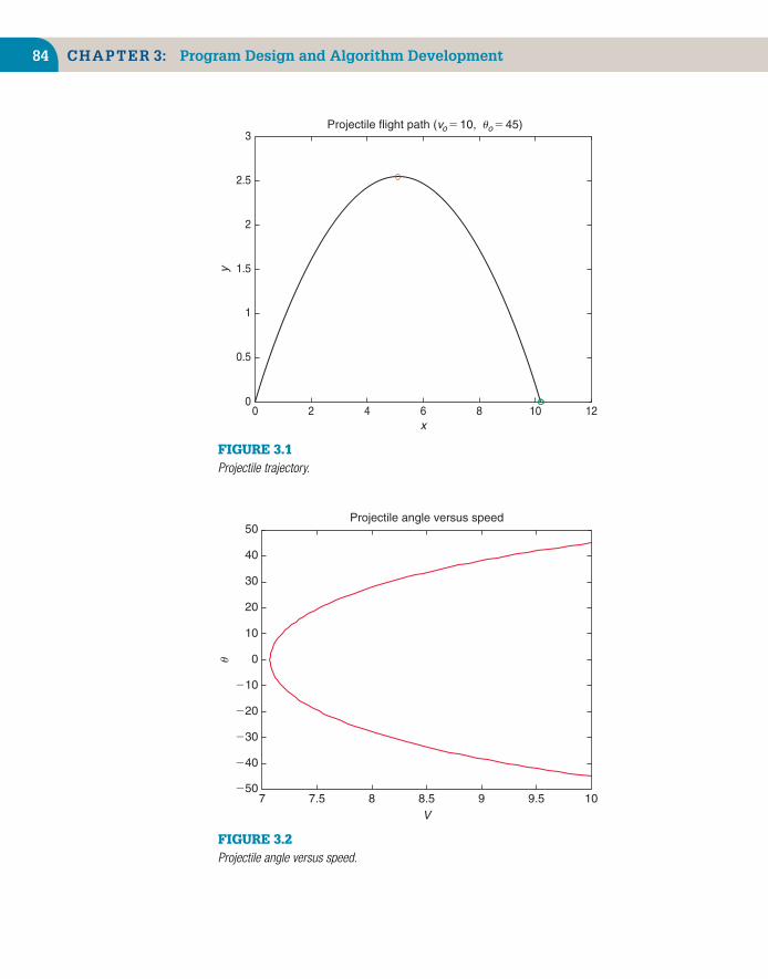
84 CHAPTER 3: Program Design and Algorithm Development
0 2 4 6 8 10 120
1
2
2.5
1.5
0.5
3 Projectile flight path (vo5 10, �o5 45)
x
y
FIGURE 3.1Projectile trajectory.
7 7.5 8 8.5 9 9.5 10250
240
230
220
210
0
10
20
30
40
50 Projectile angle versus speed
V
�
FIGURE 3.2Projectile angle versus speed.

3.2 Structure Plan Examples 85
How can you find additional examples of MATLAB programs (good ones orotherwise) to help develop tools to solve your own problems? We all recognizethat examples aren’t a bad way of learning to use tools. New tools are continuallybeing developed by the users of MATLAB. If one proves to be of more generaluse, MathWorks may include it in their list of products (if, of course, the tools’author desires this). There are also many examples of useful scripts that areplaced on the Web for anyone interested in them. They, of course, must beevaluated carefully since it is the user’s responsibility, not the creator’s, to ensurethe correctness of their results. This responsibility holds for all tools appliedby the engineer and the scientist. Hence, it is very important (just as in usinga laboratory apparatus) that users prove to themselves that the tool they areusing is indeed valid for the problem they are trying to solve.
To illustrate how easy it is to find examples of scripts, the author typedMATLAB examples in one of the available search engines and found thefollowing (among many others):
� t = (0:.1:2*pi)’;� subplot(2,2,1)� plot(t,sin(t))� subplot(2,2,2)� plot(t,cos(t))� subplot(2,2,3)� plot(t,exp(t))� subplot(2,2,4)� plot(t,1./(1+t.ˆ2))
This script illustrates how to put four plots in a single figure window. To checkthat it works, type each line in the Command Window followed by Enter. Notethe position of each graphic; location is determined by the three integers in thesubplot function list of arguments. Search Help via the question mark (?) formore information on subplot.
3.2 STRUCTURE PLAN EXAMPLES
A structure plan is typically written in what is called pseudo-code—that is, state-ments in English, mathematics, and MATLAB describing in detail how to solvea problem. You don’t have to be an expert in any particular computer languageto understand pseudo-code. A structure plan may be written at a number oflevels, each of increasing complexity, as the logical structure of the program isdeveloped.
Suppose we want to write a script to convert a temperature on the Fahren-heit scale (where water freezes and boils at 32◦ and 212◦, respectively) to the

86 CHAPTER 3: Program Design and Algorithm Development
Celsius scale. A first-level structure plan might be a simple statement of theproblem:
1. Initialize Fahrenheit temperature2. Calculate and display Celsius temperature3. Stop
Step 1 is pretty straightforward. Step 2 needs elaborating, so the second-levelplan could be something like this:
1. Initialize Fahrenheit temperature (F )2. Calculate Celsius temperature (C ) as follows:
2.1. Subtract 32 from F and multiply by 5/93. Display the value of C4. Stop
There are no hard and fast rules for writing structure plans. The essential pointis to cultivate the mental discipline of getting the problem logic clear beforeattempting to write the program. The top-down approach of structure plansmeans that the overall structure of a program is clearly thought out before youhave to worry about the details of syntax (coding). This reduces the number oferrors enormously.
A script to implement this is as follows:
% Script file to convert temperatures from F to C% D.T.V. ......... October 2006/November 2008%F = input(’ Temperature in degrees F: ’)
C = (F–32)*5/9;disp([’ Temperature in degrees C = ’,num2str(C)])% STOP
Two checks of the tool were done. They were for F = 32, which gave C = 0, andF = 212, which gave C = 100. The results were found to be correct and hencethis simple script is, as such, validated.
3.2.1 Quadratic equationWhen you were at school you probably solved hundreds of quadratic equationsof the form
ax2 + bx + c = 0
A structure plan of the complete algorithm for finding the solution(s) x, givenany values of a, b, and c, is shown in Figure 3.3. Figure 3.4 shows the graph ofa quadratic equation with real unequal roots.
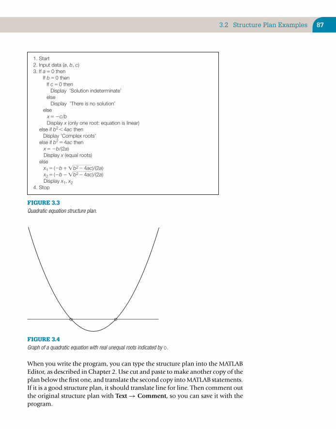
3.2 Structure Plan Examples 87
1. Start 2. Input data (a, b, c) 3. If a 5 0 then If b 5 0 then If c 5 0 then Display ’Solution indeterminate’ else Display ’There is no solution’ else x 5 2c/b Display x (only one root: equation is linear) else if b2, 4ac then Display ’Complex roots’ else if b25 4ac then x 5 2b/(2a) Display x (equal roots) else x15 (2b 1 œb22 4ac)/(2a) x25 (2b 2 œb22 4ac)/(2a) Display x1, x2 4. Stop
FIGURE 3.3Quadratic equation structure plan.
FIGURE 3.4Graph of a quadratic equation with real unequal roots indicated by o.
When you write the program, you can type the structure plan into the MATLABEditor, as described in Chapter 2. Use cut and paste to make another copy of theplan below the first one, and translate the second copy into MATLAB statements.If it is a good structure plan, it should translate line for line. Then comment outthe original structure plan with Text → Comment, so you can save it with theprogram.

88 CHAPTER 3: Program Design and Algorithm Development
3.3 STRUCTURED PROGRAMMING WITHFUNCTIONS
Many examples later in this book will be rather involved. More advanced pro-grams like these should be structured by means of your own function M-files.These are dealt with in detail in Chapter 10. A function M-file is a script file(i.e., a file with an .m extension) that you can “call” interactively, or from otherscripts, in specific ways.
The “main” script will look very much like a first-level structure plan of theproblem. For example, the quadratic equation problem may be structure-planned at the first level as follows:
1. Input the data2. Find and display the solution(s)3. Stop
Using a function file that you created and called quadratic.m to do the dirtywork could be translated directly into the following MATLAB script:
a = input( ’Enter coefficients: ’ );x = quadratic(a);
(The details on coding this particular problem are left as an exercise inChapter 10.)
SUMMARY
■ An algorithm is a systematic logical procedure for solving a problem.
■ A structure plan is a representation of an algorithm in pseudo-code.
■ A function M-file is a script file designed to handle a particular task thatmay be activated (invoked) whenever needed.
CHAPTER EXERCISES
The problems in these exercises should all be structure-planned before being written up asMATLAB programs (where appropriate).
3.1. The structure plan in this example defines a geometric construction. Carry out the plan
by sketching the construction:
1. Draw two perpendicular x- and y-axes2. Draw the points A (10, 0) and B (0, 1)3. While A does not coincide with the origin repeat:
Draw a straight line joining A and B

Summary 89
Move A one unit to the left along the x-axisMove B one unit up on the y-axis
4. Stop
3.2. Consider the following structure plan, where M and N represent MATLAB variables:
1. Set M = 44 and N = 282. While M not equal to N repeat:
While M > N repeat:Replace value of M by M – N
While N > M repeat:Replace value of N by N – M
3. Display M4. Stop
(a) Work through the structure plan, sketching the contents of M and N duringexecution. Give the output.
(b) Repeat (a) for M = 14 and N = 24.
(c) What general arithmetic procedure does the algorithm carry out (try more valuesof M and N if necessary)?
3.3. Write a program to convert a Fahrenheit temperature to Celsius. Test it on the data inExercise 2.11 (where the reverse conversion is done).
3.4. Write a script that inputs any two numbers (which may be equal) and displays the largerone with a suitable message or, if they are equal, displays a message to that effect.
3.5. Write a script for the general solution to the quadratic equation ax 2 + bx + c = 0.Use the structure plan in Figure 3.3. Your script should be able to handle all possiblevalues of the data a, b, and c . Try it out on the following values:
(a) 1, 1, 1 (complex roots)
(b) 2, 4, 2 (equal roots of −1.0)
(c) 2, 2, −12 (roots of 2.0 and −3.0)
The structure plan in Figure 3.3 is for programming languages that cannot handlecomplex numbers. MATLAB can. Adjust your script so that it can also find complexroots. Test it on case (a); the roots are −0.5 ± 0.866i .
(Continued)
3.6. Develop a structure plan for the solution to two simultaneous linear equations (i.e.,the equations of two straight lines). Your algorithm must be able to handle all possiblesituations; that is, lines intersecting, parallel, or coincident. Write a program toimplement your algorithm, and test it on some equations for which you know thesolutions, such as
x + y = 3
2x − y = 3
(x = 2, y = 1). Hint : Begin by deriving an algebraic formula for the solution to thesystem:
ax + by = c
dx + ey = f
The program should input the coefficients a, b, c , d , e, and f .

90 CHAPTER 3: Program Design and Algorithm Development
We will see in Chapter 16 that MATLAB has a very elegant way of solving systems ofequations directly, using matrix algebra. However, it is good for the development ofyour programming skills to do it the long way, as in this exercise.
3.7. We wish to examine the motion of a damped harmonic oscillator. The small ampli-tude oscillation of a unit mass attached to a spring is given by the formulay = e−(R/2)t sin(ω1t ), where ω2
1 = ω2o − R2/4 is the square of the natural frequency of
the oscillation with damping (i.e., with resistance to motion); ω2o = k is the square of
the natural frequency of undamped oscillation; k is the spring constant; and R is thedamping coefficient. Consider k = 1 and vary R from 0 to 2 in increments of 0.5. Ploty versus t for t from 0 to 10 in increments of 0.1. Hint : Develop a solution procedureby working backwards through the problem statement. Starting at the end of theproblem statement, the solution procedure requires the programmer to assign theinput variables first followed by the execution of the formula for the amplitude andending with the output in graphical form.
3.8. Let’s examine the shape of a uniform cable hanging under its own weight. The shapeis described by the formula y = cosh(x/c ). This shape is called a uniform catenary.The parameter c is the vertical distance from y = 0 where the bottom of the catenaryis located. Plot the shape of the catenary between x = −10 and x = 10 for c = 5.Compare this with the same result for c = 4. Hint : The hyperbolic cosine, cosh, is abuilt-in MATLAB function that is used in a similar way to the sine function, sin.

CHAPTER 4
MATLAB Functions and Data Import–ExportUtilities
The objectives of this chapter are
■ To enable you to become familiar with some of the more commonMATLAB functions
■ To introduce you to ways of importing and exporting data in and outof the MATLAB workspace using the load and save command, theImport Wizard, and the low-level file input/output (I/O) functions
At this point you should be able to write a MATLAB program that inputs data,performs simple arithmetic operations on it, perhaps involving loops and deci-sions, and displays the results of the computation in a comprehensible form.However, more interesting problems in science and engineering are likely toinvolve special mathematical functions like sines, cosines, logarithms, and thelike. MATLAB comes with a large collection of such functions; we have seensome of them already. This chapter introduces you to the more common func-tions available in MATLAB. In addition, because you may wish to import datato be plotted or operated on mathematically, and export data for future use,the chapter also introduces you to the importing of data into the MATLABworkspace from various sources and discusses the exporting of data to files inyour working directory.
4.1 COMMON FUNCTIONS
Tables of MATLAB functions and commands appear in Appendix C. A shortlist of some of the more common ones follows. Use helpwin at the commandline to see a list of categories of functions, with links to their descriptions.
Copyright © 2010, Daniel T. Valentine. Published by Elsevier Ltd. All rights reserved.DOI: 10.1016/B978-0-12-374883-6.00004-7 91

92 CHAPTER 4: MATLAB Functions and Data Import–Export Utilities
Alternatively, go to the Contents listing in the Help Navigator (the left panein the Help browser) and expand successively MATLAB, Reference, MATLABFunction Reference, where you can choose either Functions by Category orAlphabetical List of Functions.
Note that if the argument of a function is an array, the function is appliedelement by element to all the values in the array. For example,
sqrt([1 2 3 4])
returns
1.0000 1.4142 1.7321 2.0000
Since this text is written in a tutorial style, it is expected that you will examinethe following list of common MATLAB functions. It is also expected that youalready know, from your first courses in mathematics and science, somethingabout them. One way to examine these functions is to plot them. Have some funexperimenting with MATLAB in your investigation of the following functions.For example, do the following exercise for all functions of the assigned variablex, as illustrated next.
x = –1:.1:1; <Enter>plot(x,abs(x),’o’) <Enter>
You should get an illustration that looks like a V.
abs(x) absolute value of x.
acos(x) arc cosine (inverse cosine) of x between 0 and π.
acosh(x) inverse hyperbolic cosine of x, or ln(x + √x2 − 1).
asin(x) arc sine (inverse sine) of x between −π/2 and π/2.
asinh(x) inverse hyperbolic sine of x, or ln(x + √x2 + 1).
atan(x) arc tangent of x between −π/2 and π/2.
atan2(y, x) arc tangent of y/x between −π and π.
atanh(x) inverse hyperbolic tangent of x, or12
ln(
1 + x1 − x
).
ceil(x) smallest integer that exceeds x (rounds up to the near-est integer)—for example, ceil(–3.9) returns –3; ceil(3.9) returns 4.
clock time and date in a six-element vector—for example, thestatements

4.1 Common Functions 93
t = clock;fprintf( ’ %02.0f:%02.0f:%02.0f\n’,t(4), t(5), t(6) );
result in 14:09:03. Note how the hours, minutes, andseconds are left-filled with zeros if necessary.
cos(x) cosine of x.
cosh(x) hyperbolic cosine of x, orex + e−x
2(see Figure 4.1).
cot(x) cotangent of x.
csc(x) cosecant of x.
cumsum(x) cumulative sum of the elements of x (e.g., cumsum(1:4)returns [1 3 6 10]).
date date in a string in dd-mmm-yyyy format (e.g., 02-Feb-2001).
exp(x) value of the exponential function ex (see Figure 4.1).
fix(x) rounds to the nearest integer toward zero (e.g.,fix(–3.9)returns –3; fix(3.9) returns 3).
floor(x) largest integer not exceeding x—that is, rounds down tonearest integer (e.g., floor(–3.9) returns –4; floor(3.9) returns 3).
0 0.5 1 1.5 222 21.5 21 20.524
22
0
2
4
6
8
(c)
(b)
(a)
FIGURE 4.1(a) Exponential, (b) hyperbolic sine, and (c) hyperbolic cosine functions.

94 CHAPTER 4: MATLAB Functions and Data Import–Export Utilities
length(x) number of elements in vector x.
log(x) natural logarithm of x.
log10(x) base 10 logarithm of x.
max(x) maximum element of vector x.
mean(x) mean value of elements in vector x.
min(x) minimum element in vector x.
pow2(x) 2x.
prod(x) product of the elements of x.
rand pseudo-random number in the interval [0, 1). The valuereturned is pseudo-random rather than truly random inthe sense that there is an algorithm that determines randfrom the initial “seed.” The same seed will generate thesame “random” sequence (see Chapter 15 for how to seedrand by looking in the index).
realmax largest positive floating-point number on your computer.
realmin smallest positive floating-point number on your com-puter.
rem(x, y) remainder when x is divided by y—for example, rem(19,5) returns 4 (5 goes 3 times into 19, remainder 4). Strictly,rem(x, y) returns x – y * n, where n = fix(x/y) isthe integer nearest tox/y. This shows how negative and/ornoninteger arguments are handled. rem and fix are use-ful for converting smaller units to larger ones, say inchesto feet and inches (one foot = 12 inches). The followingstatements convert 40 inches this way:
feet = fix(40/12)inches = rem(40, 12)
Let’s next look at an example that will hopefully inspire you to examine allof the functions listed as well as any other MATLAB function you may dis-cover. We will consider arc-cosine, arc-sine, and arc-tangent: acos(x), acos(x),and atan(x), respectively. If you specify x—that is, the cosine, the sine, andthe tangent, respectively, between –1 and 1—in what quadrant of the circleare the output angles selected? To provide an answer, the following M-filescript was created and executed. The graphical comparison of the computedresults is illustrated in Figure 4.2. REMARKS at the end of the script provides

4.1 Common Functions 95
2100 250 0 50 100 150 20021
20.8
20.6
20.4
20.2
0
0.2
0.4
0.6
0.8
1
� in (degrees)
x (a
rgum
ent o
f the
func
tion)
asin(x)acos(x)atan(x)
FIGURE 4.2Comparison of results from the acos, asin, and atan functions.
an interpretation of the graphical results and hence an answer to the questionraised.
%% Script to compare the acos(x), asin(x), and atan(x)% functions over the range –1 < x < 1. The values are% converted to angles in degrees. The results are% compared graphically.%% Script prepared by D. T. Valentine – September 2006.% Comments modified by D.T.V. ......... November 2008.%% The question raised is: What range of angles, i.e.,% which of the four quadrants of the circle from 0 to% 2*pi are the angular outputs of each of the functions?%% Assign the values of x to be examined:%x = –1:0.001:1;%% Compute the arc-functions:%y1 = acos(x);

96 CHAPTER 4: MATLAB Functions and Data Import–Export Utilities
y2 = asin(x);y3 = atan(x);%% Convert the angles from radians to degrees:%y1 = 180*y1/pi;y2 = 180*y2/pi;y3 = 180*y3/pi;%% Plot the results:%plot(y1,x,y2,x,y3,x),gridlegend(’asin(x)’, ’acos(x)’, ’atan(x)’)xlabel(’\theta in degrees’)ylabel(’x, the argument of the function’)%% REMARKS: Note the following:% (1) The acos(x) varies from 0 to 90 to 180 degrees.% (2) The asin(x) varies from –90 to 0 to 90 degrees.% (3) The atan(x) varies from –90 to 0 to 90 degrees.% To check remark (3) try atan(1000000)*180/pi.%% Stop
4.2 IMPORTING AND EXPORTING DATA
When you get into serious programming, you will often need to store data ona disk. The process of moving data between MATLAB and disk files is calledimporting (from disk files) and exporting (to disk files). Data is saved in diskfiles in one of two formats: text and binary. In text format, data values are ASCIIcodes and can be viewed in any text editor. In binary format, they are not ASCIIcodes and cannot be viewed in a text editor. Binary format is more efficient interms of storage space required.
This section provides a brief summary of the main ways in which MATLABimports and exports data. For full details consult MATLAB Help: DevelopmentEnvironment: Importing and Exporting Data.
4.2.1 The load and save commandsIf you want to save data between MATLAB sessions, save and load are probablythe best commands to use.

4.2 Importing and Exporting Data 97
4.2.2 Exporting text (ASCII) dataTo export (save) the array
A =1 2 34 5 6
in “delimited” ASCII format in the file myData.txt, use the command
save myData.txt A –ascii
If you view myData.txt in a text editor (or type it in the Command Window)it looks like this:
1.0000000e+000 2.0000000e+000 3.0000000e+0004.0000000e+000 5.0000000e+000 6.0000000e+000
Delimiters are the characters used to separate the data values in the file—spacesby default. You can use tabs instead of spaces by specifying the –tabs qualifierinstead of –ascii. If you save character arrays (strings) in this way, the ASCIIcodes of the characters are written to the file.
4.2.3 Importing text (ASCII) dataThe load command is the reverse of save, but has a curious twist. If the arrayA has been saved in myData.txt as above, the command
load myData.txt
creates a variable in the workspace with the same name as the file, minus theextension: myData. If you don’t want the filename as the variable name, use thefunctional form of the command:
A = load(’myData.txt’)
Data imported in this way doesn’t have to be created by MATLAB. You can createit in a text editor in any other program that exports data in ASCII format.
4.2.4 Exporting and importing binary dataThe command
save filename x y z
saves the variables x, y, and z in the file filename.mat in MATLAB proprietarybinary format—that is, a file that can only be used by MATLAB.

98 CHAPTER 4: MATLAB Functions and Data Import–Export Utilities
Note:
■ If no variables are listed, the entire workspace is saved.
■ The extension .mat is the default—you can specify a different extension.
■ Seek Help for all save options.
The command
load filename
loads all the variables from filename.mat into the workspace; see Help for allload options.
4.2.5 The Import WizardThe MATLAB Import Wizard is the easiest way of importing data into theworkspace during an interactive session.
Importing ASCII dataImport ASCII data with the Import Wizard as follows:
1. Start the Import Wizard by selecting Import Data on the MATLAB Filemenu. You can also type uiimport on the command line. A list of filesappears in a dialogue box. Open the file you want to import.
2. Select the delimiter used in the text file (if necessary). Click Next.
3. Select the variables you want to import. By default the Import Wizardputs all numeric data in one variable and all text data in other variables,but you can choose other options.
4. Click Finish to import the data into the selected variables.
Importing binary dataTo import binary data with the Import Wizard, start in the same way as whenimporting text data. When the file opens, the Import Wizard attempts to processits contents and creates variables depending on the type of data in it. Checkthe variables you want to import and click Finish to create them. You can,for example, import data from an Excel spreadsheet in this way. If the data isnumeric with row and column headers, the Import Wizard imports it into anumeric array and the headers into a cell array.
4.2.6 *Low-level file I/O functionsMATLAB has a set of low-level file I/O (input/output) functions based on theI/O functions of the ANSI Standard C Library. You would typically use these

4.2 Importing and Exporting Data 99
functions to access binary data written in C or Java, for example, or to access adatabase that is too large to be loaded into the workspace in its entirety.
C programmers should note that not all MATLAB file I/O commands are identi-cal to their C counterparts. For example, fread is “vectorized”—that is, it readsuntil it encounters a text string or the end of a file.
Files can be accessed with low-level I/O functions in text or binary mode. Inbinary mode you can think of the file as a long continuous stream of bytes,which are your responsibility to interpret correctly. Files opened in binary modecan be accessed “randomly”—that is, you can specify at which particular byteyou want to start reading or writing.
The short programs that follow show how to create a file in binary mode, howto read it, and how to change it. Explanations of new features follow each one.You will need to consult the online documentation and Help to see the widerange of options available for these I/O functions.
Writing binary dataThe example we are going to use has a wide variety of applications. We want toset up a database of records, each consisting of information about individuals(clients, customers, students). In this example each record will have a student’sname and one mark. (The term record has no particular significance in MATLAB,as it does, for example, in Pascal. It is used here as a convenient way of thinkingabout the basic unit in a database.)
The following program (writer.m) invites you to enter any number of namesand marks from the command line and then writes them as binary data to afile. To terminate the process, hit Enter for the next name.
namelen = 10; % 10 bytes for namefid = fopen(’marks.bin’, ’w’); % open for write onlystr = ’?’; % not empty to start
while ˜isempty(str)str = input( ’Enter name: ’, ’s’ );if ˜isempty(str)
if length(str) > namelenname = str(1:namelen); %only first ten chars allowed
elsename = str;name(length(str)+1:namelen) = ’ ’; %pad with blanks if
...too shortendfwrite(fid, name);

100 CHAPTER 4: MATLAB Functions and Data Import–Export Utilities
mark = input( ’Enter mark: ’ );fwrite(fid, mark, ’float’); % 4 bytes for mark
endend
fclose(fid);
Note that
■ The statement
fid = fopen(’marks.bin’, ’w’);
creates a file marks.bin for writing only. If the file is successfullyopened, fopen returns a nonnegative integer called the file identifier(fid), which can be passed to other I/O functions to access the openedfile. If fopen fails (e.g., if you try to open a nonexistent file for reading),it returns –1 to fid and assigns an error message to an optional secondoutput argument. The second argument, ’w’, of fopen is the permissionstring and specifies the kind of access to the file you require (e.g., ’r’ forread only, ’w’ for write only, ’r+’ for both reading and writing, etc.).See help fopen for all possible permission strings.
■ The while loop continues asking for names until an empty string isentered (str must therefore be nonempty initially).
■ Each name written to the file must be the same length (otherwise youwon’t know where each record begins when it comes to changing it).The if statement ensures that each name has exactly 10 characters(namelen) no matter how many characters are entered (the number 10is arbitrary of course!).
■ The first fwrite statement
fwrite(fid, name);
writes all the characters in name to the file (one byte each).
■ The second fwrite statement
fwrite(fid, mark, ’float’);
writes mark to the file. The third (optional) argument (precision)specifies both the number of bits written for mark and how they willbe interpreted in an equivalent fread statement. ’float’ meanssingle-precision numeric (usually 32 bits—4 bytes—although thisvalue is hardware dependent). The default for this argument is’uchar’—unsigned characters (1 byte).

4.2 Importing and Exporting Data 101
■ The statement
fclose(fid);
closes the file (returning 0 if the operation succeeds). Although MATLABautomatically closes all files when you exit, it is good practice to closefiles explicitly with fclose when you have finished using them.Note that you can close all files with fclose(’all’).
Reading binary dataThe next program (reader.m) reads the file written with writer.m and displayseach record:
namelen = 10; % 10 bytes for namefid = fopen(’marks.bin’, ’r’);
while ˜feof(fid)str = fread(fid,namelen);name = char(str’);mark = fread(fid, 1, ’float’);fprintf(’%s %4.0f\n’, name, mark)
end
fclose(fid);
Note the following:
■ The file is opened for read only (’r’).
■ The function feof(fid) returns 1 if the end of the specified file hasbeen reached, and 0 otherwise.
■ The first fread statement reads the next namelen (10) bytes from thefile into the variable str. When the name was written by fwrite, theASCII codes of the characters were actually written to the file. Therefore,the char function is needed to convert the codes back to characters.Furthermore, the bytes being read are interpreted as entries in a columnmatrix; str must be transposed if you want to display the name in theusual horizontal format.
■ The second fread statement specifies that one value (the number ofvalues is given by the second argument) is to be read in float precision(four bytes). You can, for example, read an entire array of 78 floatnumbers with
a = fread(fid, 78, ’float’);

102 CHAPTER 4: MATLAB Functions and Data Import–Export Utilities
Changing binary dataTo demonstrate how to change records in a file, we assume for simplicity thatyou will only want to change a student’s mark, not the name. The program below(changer.m) asks which record to change, displays the current name and markin that record, asks for the corrected mark, and overwrites the original mark.
namelen = 10; % 10 bytes for namereclen = namelen + 4;fid = fopen(’marks.bin’, ’r+’); % open for read and write
rec = input( ’Which record do you want to change? ’ );fpos = (rec–1)*reclen; % file position indicatorfseek(fid, fpos, ’bof’); % move file position indicatorstr = fread(fid,namelen); % read the namename = char(str’);mark = fread(fid, 1, ’float’); % read the markfprintf(’%s %4.0f\n’, name, mark)
mark = input(’Enter corrected mark: ’); % new markfseek(fid, –4, ’cof’); % go back 4 bytes to start of markfwrite(fid, mark, ’float’); % overwrite markfprintf( ’Mark updated’ );
fclose(fid);
Note the following:
■ The file is opened for reading and writing (’r+’).
■ When a file is opened with fopen, MATLAB maintains a file positionindicator. The position in the file where MATLAB will begin the nextoperation (reading or writing) is one byte beyond the file positionindicator.
fpos calculates the value of the file position indicator in order tocommence reading the record number, rec.
■ The fseek function moves the file position indicator. Its secondargument specifies where in the file to move the indicator relative to anorigin given by the third argument. Possible origins are ’bof’(beginning of file), ’cof’ (current position in file) and ’eof’ (endof file).
In this example, the records are 14 bytes long (10 for the name, 4 for themark). If we want to update the second record, we use
fseek(fid, 14, ’bof’);

Summary 103
which moves the file position indicator to byte 14 from the beginning ofthe file, ready to start accessing at byte 15, which is the beginning of thesecond record. The function fseek returns 0 (successful) or –1(unsuccessful). Incidentally, if you get lost, you can always used ftellto find out where you are!
■ The fread statement, which reads the mark to be changed,automatically advances the file position indicator by four bytes (thenumber of bytes required by float precision). In order to overwrite themark, we therefore have to move the file position indicator back fourbytes from its current position, The statement
fseek(fid, –4, ’cof’);
achieves this.
■ The fwrite statement then overwrites the mark.
The programs above have no error-trapping devices that, for example, preventyou from reading from a nonexistent file or prevent you from overwriting arecord that isn’t there. It is left to you to fill in these sorts of details.
4.2.7 *Other import/export functionsOther import/export functions, with differing degrees of flexibility and ease ofuse, include csvread, csvwrite, dlmread, dlmwrite, fgets, fprintf (whichhas an optional argument to specify a file), fscanf, textread, xlsread. Youknow where to look for the details.
Finally, recall that the diary command can also be used to export small arraysas text data, although you will need to edit out extraneous text.
SUMMARY
■ MATLAB functions may be used to perform mathematical, trigonometric,and other operations.
■ Data can be saved to disk files in text (ASCII) format or in binary format.
■ load and save can be used to import/export both text and binary data (thelatter in the form of MAT-files).
■ The Import Wizard provides an easy way of importing both text and binarydata.
■ MATLAB’s low-level I/O functions such as fread and fwrite providerandom access to binary files.

104 CHAPTER 4: MATLAB Functions and Data Import–Export Utilities
CHAPTER EXERCISES
4.1. Write some MATLAB statements that will(a) Find the length C of the hypotenuse of a right-angle triangle in terms of the
lengths A and B of the other two sides.
(b) Find the length C of a side of a triangle given the lengths A and B of the othertwo sides and the size in degrees of the included angle θ, using the cosine rule:
C 2 = A2 + B2 − 2AB cos(θ).
4.2. Translate the following formulae into MATLAB expressions:(a) ln(x + x 2 + a2)
(b) [e3t + t2 sin(4t )] cos2(3t )
(c) 4 tan−1(1) (inverse tangent)
(d) sec2(x ) + cot(y )
(e) cot−1(|x/a|) (use MATLAB’s inverse cotangent)
4.3. There are 39.37 inches in a meter, 12 inches in a foot, and 3 feet in a yard. Write a scriptto input a length in meters (which may have a decimal part) and convert it to yards, feet,and inches. (Check: 3.51 m converts to 3 yds, 2 ft, 6.19 in.)
4.4. A sphere of mass m1 impinges obliquely on a stationary sphere of mass m2, the directionof the blow making an angle α with the line of motion of the impinging sphere. If thecoefficient of restitution is e, it can be shown that the impinging sphere is deflectedthrough an angle β such that
tan(β) = m2(1 + e)tan(α)
m1 − em2 + (m1 + m2)tan2(α)
Write a script to input values of m1, m2, e, and α (in degrees) and to compute the angleβ in degrees.
4.5. Section 2.7 has a program for computing the members of the sequence xn = an/n. Itdisplays every member xn computed. Adjust it to display only every tenth value of xn .Hint: the expression rem(n, 10) will be zero only when n is an exact multiple of 10.Use this in an if statement to display every tenth value of xn .
4.6. To convert the variablemins,minutes, into hours and minutes,you usefix(mins/60)to find the whole number of hours and rem(mins, 60) to find the number of minutesleft over. Write a script that inputs a number of minutes and converts it to hours andminutes.Then write a script to convert seconds into hours,minutes,and seconds.Tryouton 10,000 seconds, which should convert to 2 hours 46 minutes, and 40 seconds.
4.7. Design an algorithm (i.e., write the structure plan) for a machine that must give thecorrect amount of change from a $100 bill for any purchase costing less than $100. Theplan must specify the number and type of all bills and coins in the change, and shouldin all cases give as few bills and coins as possible. (If you are not familiar with dollarsand cents, use your own monetary system.)
4.8. A uniform beam is freely hinged at its ends, x = 0 and x = L, so that the ends are atthe same level. It carries a uniformly distributed load of W per unit length, and there is

Summary 105
a tension, T , along the x -axis. The deflection, y , of the beam a distance, x , from one endis given by
y = WEIT 2
[cosh[a(L/2 − x )]
cosh(aL/2)− 1
]+ Wx (L − x )
2T
where a2 = T /EI , E being theYoung’s modulus of the beam and I the moment of inertiaof a cross-section of the beam. The beam is 10 m long, the tension is 1000 N, the load is100 N/m, and EI is 104.
Write a script to compute and plot a graph of the deflection y against x (MATLAB hasa cosh function). To make the graph look realistic you will have to override MATLAB’sautomatic axis scaling with the statement
axis( [xmin xmax ymin ymax] )
after the plot statement, where xmin and so forth have appropriate values.

CHAPTER 5
Logical Vectors
The objectives of this chapter are to enable you to
■ Understand logical operators more fully
And to introduce you to
■ Logical vectors and how to use them effectively in a number ofapplications
■ Logical functions
This chapter introduces a most powerful and elegant feature of MATLAB, logicalvectors. The topic is so useful and hence important that it deserves a chapter ofits own.
As an exercise, enter the following statements on the command line:
r = 1;r <= 0.5 % no semi-colon
If you correctly left out the semicolon after the second statement, you will havenoticed that it returned the value 0. Now enter the expression r >= 0.5 (again,no semicolon). It should return the value 1. We already saw in Chapter 2 thata logical expression in MATLAB involving only scalars returns a value of 0 if itis FALSE and 1 if it is TRUE.
If you enter
r = 1:5;r <= 3
Copyright © 2010, Daniel T. Valentine. Published by Elsevier Ltd. All rights reserved.DOI: 10.1016/B978-0-12-374883-6.00005-9 107
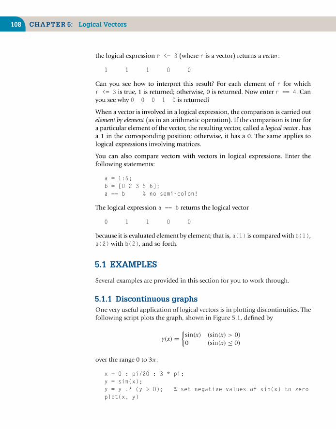
108 CHAPTER 5: Logical Vectors
the logical expression r <= 3 (where r is a vector) returns a vector:
1 1 1 0 0
Can you see how to interpret this result? For each element of r for whichr <= 3 is true, 1 is returned; otherwise, 0 is returned. Now enter r == 4. Canyou see why 0 0 0 1 0 is returned?
When a vector is involved in a logical expression, the comparison is carried outelement by element (as in an arithmetic operation). If the comparison is true fora particular element of the vector, the resulting vector, called a logical vector, hasa 1 in the corresponding position; otherwise, it has a 0. The same applies tological expressions involving matrices.
You can also compare vectors with vectors in logical expressions. Enter thefollowing statements:
a = 1:5;b = [0 2 3 5 6];a == b % no semi-colon!
The logical expression a == b returns the logical vector
0 1 1 0 0
because it is evaluated element by element; that is, a(1) is compared with b(1),a(2) with b(2), and so forth.
5.1 EXAMPLES
Several examples are provided in this section for you to work through.
5.1.1 Discontinuous graphsOne very useful application of logical vectors is in plotting discontinuities. Thefollowing script plots the graph, shown in Figure 5.1, defined by
y(x) ={
sin(x) (sin(x) > 0)
0 (sin(x) ≤ 0)
over the range 0 to 3π:
x = 0 : pi/20 : 3 * pi;y = sin(x);y = y .* (y > 0); % set negative values of sin(x) to zeroplot(x, y)

5.1 Examples 109
00
0.2
0.4
0.6
0.8
1
1.2
1.4
1.6
1.8
2
1 2 3 4 5 6 7 8 9 10
FIGURE 5.1Discontinuous graph using logical vectors.
The expression y > 0 returns a logical vector with 1s where sin(x) is positiveand 0s otherwise. Element-by-element multiplication by y with .* then picksout the positive elements of y.
5.1.2 Avoiding division by zeroSuppose you want to plot the graph of sin(x)/x over the range −4π to 4π. Themost convenient way to set up a vector of the x coordinates is
x = –4*pi : pi / 20 : 4*pi;
But then, when you try
y = sin(x) ./ x;
you get the Divide by zero warning because one of the elements of x isexactly zero. A neat way around this problem is to use a logical vector to replacethe zero with eps. This MATLAB function returns the difference between 1.0and the next largest number that can be represented in MATLAB, which isapproximately 2.2e–16. Here is how to do it:
x = x + (x == 0)*eps;
The expression x == 0 returns a logical vector with a single 1 for the elementof x that is zero, and so eps is added only to that element. The following

110 CHAPTER 5: Logical Vectors
20.4215 210 25 50 10 15
0.4
0.6
0.8
1
20.2
0.2
0
FIGURE 5.2sin(x)/x.
script plots the graph correctly—without a missing segment at x = 0 (seeFigure 5.2).
x = –4*pi : pi/20 : 4*pi;x = x + (x == 0)*eps; % adjust x = 0 to x = epsy = sin(x) ./ x;plot(x, y)
When x has the value eps, the value of sin(eps)/eps has the correct limitingvalue of 1 (check it) instead of NaN (Not-a-Number) resulting from a divisionby zero.
5.1.3 Avoiding infinityThe following script attempts to plot tan(x) over the range −3π/2 to 3π/2. Ifyou are not experienced with trig graphs, perhaps you should sketch the graphroughly with pen and paper before you run the script!
x = –3/2*pi : pi/100 : 3/2*pi;y = tan(x);plot(x, y)
The MATLAB plot (Figure 5.3(a)) should look nothing like your sketch. Theproblem is that tan(x) approaches ±∞ at odd multiples of π/2. The scale onthe MATLAB plot is therefore very large (about 1015), making it impossible tosee the structure of the graph anywhere else.

5.1 Examples 111
1
0.5
20.5
25 521
0
0
40
20
220
25 5240
0
0
(a) (b)
3 1016
FIGURE 5.3Variations on tan(x): (a) Unrestricted vertical coordinate. (b) Restricted vertical coordinate.
If you add the statement
y = y .* (abs(y) < 1e10); % remove the big ones
just before the plot statement, you get a much nicer graph, as shown inFigure 5.3(b). The expression abs(y) < 1e10 returns a logical vector that iszero only at the asymptotes. The graph thus goes through zero at these points,which incidentally draw nearly vertical asymptotes for you that become morevertical as the increment in x becomes smaller.
5.1.4 Counting random numbersThe function rand returns a (pseudo-)random number in the interval [0, 1);rand(1, n) returns a row vector of n such numbers. Work out the followingproblem on the command line:
1. Set up a vector r with seven random elements (leave out the semicolonso that you can see its elements):
r = rand(1,7) % no semi-colon
Check that the logical expression r < 0.5 gives the correct logical vector.
2. Using the function sum on the logical expression r < 0.5will effectivelycount how many elements of r are less than 0.5. Try it and check youranswer against the values displayed for r:
sum( r < 0.5 )
3. Now use a similar statement to count how many elements of r are greaterthan or equal to 0.5 (the two answers should add up to 7).

112 CHAPTER 5: Logical Vectors
4. Since rand generates uniformly distributed random numbers, you wouldexpect the number of random numbers less than 0.5 to get closer andcloser to half the total number as more and more are generated. Generatea vector of a few thousand random numbers (suppress display with asemicolon this time) and use a logical vector to count how many are lessthan 0.5. Repeat a few times, with a new set of random numbers eachtime. Because the numbers are random, you should never get quite thesame answer.
Without logical vectors this problem is a little more involved. Here is theprogram:
tic % starta = 0; % number >= 0.5b = 0; % number < 0.5
for n = 1:5000r = rand; % generate one number per loopif r >= 0.5a = a + 1;
elseb = b + 1;
end;end;
t = toc; % finishdisp( [’less than 0.5: ’ num2str(a)] )disp( [’time: ’ num2str(t)] )
It also takes longer. Compare times for the two methods on your computer.
5.1.5 Rolling diceWhen a fair die is rolled, the number uppermost is equally likely to be anyinteger from 1 to 6. Thus, if rand is a random number in the range [0, 1),6 * rand will be in the range [0, 6) and 6 * rand + 1 will be in the range[1, 7), that is, between 1 and 6.9999. Discarding the decimal part of thisexpression with floor gives an integer in the required range.
Try the following:
1. Generate a vector d of 20 random integers in the range 1 to 6:
d = floor(6 * rand(1, 20)) + 1
2. Count the number of “sixes” thrown by summing the elements of thelogical vector d == 6.

5.2 Logical Operators 113
3. Verify your result by displaying d.
4. Estimate the probability of throwing a six by dividing the number ofsixes thrown by 20. Using random numbers like this to mimic a realsituation based on chance is called simulation.
5. Repeat with more random numbers in the vector d. The more you have,the closer the proportion of sixes gets to the theoretical expected valueof 0.1667 (i.e., 1/6).
6. Can you see why it would be incorrect to use round instead of floor?The problem is that round rounds in both directions, whereas floorrounds everything down.
5.2 LOGICAL OPERATORS
We saw briefly in Chapter 2 that logical expressions can be constructed not onlyfrom the six relational operators but also from the three logical operators shownin Table 5.1. Table 5.2 shows the effects of these operators on the general logicalexpressions lex1 and lex2.
The OR operator (|) is technically inclusive because it is true when either orboth of its operands are true. MATLAB also has an exclusive OR function,xor(a, b), which is 1 (true) only when either of a and b, but not both, is1 (Table 5.2).
MATLAB also has a number of functions that perform bitwise logical operations.See Help on ops.
Table 5.1 Logical Operators
Operator Meaning
˜ NOT& AND| OR
Table 5.2 Truth Table
lex1 lex2 ˜lex1 lex1 & lex2 lex1 | lex2 xor(lex1, lex2)
F F T F F FF T T F T TT F F F T TT T F T T F
T = true; F = false
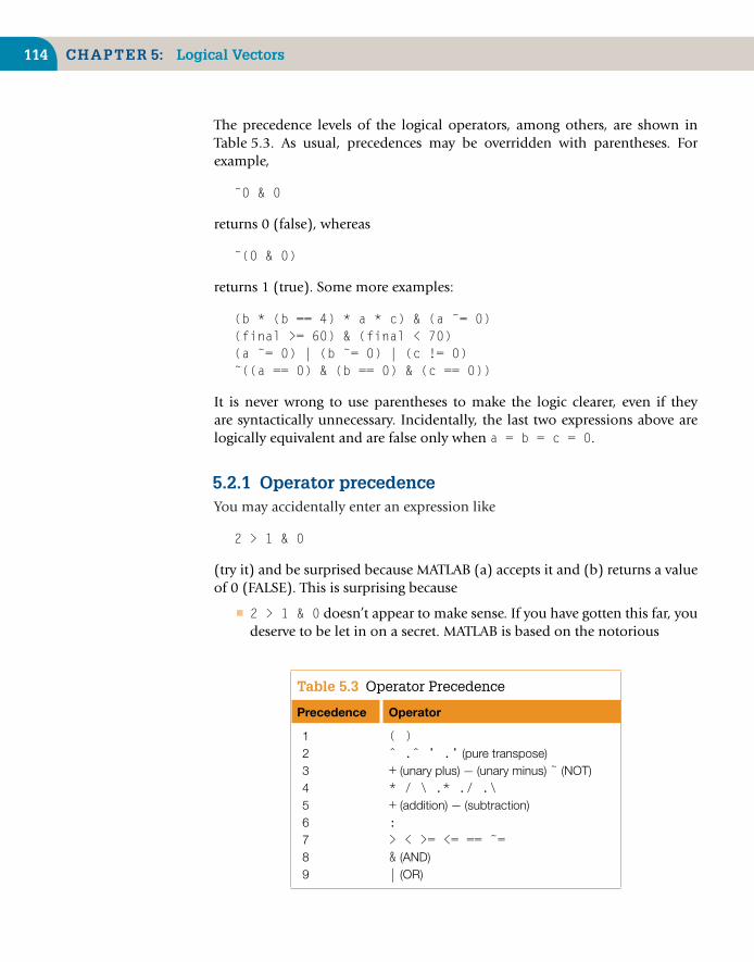
114 CHAPTER 5: Logical Vectors
The precedence levels of the logical operators, among others, are shown inTable 5.3. As usual, precedences may be overridden with parentheses. Forexample,
˜0 & 0
returns 0 (false), whereas
˜(0 & 0)
returns 1 (true). Some more examples:
(b * (b == 4) * a * c) & (a ˜= 0)(final >= 60) & (final < 70)(a ˜= 0) | (b ˜= 0) | (c != 0)˜((a == 0) & (b == 0) & (c == 0))
It is never wrong to use parentheses to make the logic clearer, even if theyare syntactically unnecessary. Incidentally, the last two expressions above arelogically equivalent and are false only when a = b = c = 0.
5.2.1 Operator precedenceYou may accidentally enter an expression like
2 > 1 & 0
(try it) and be surprised because MATLAB (a) accepts it and (b) returns a valueof 0 (FALSE). This is surprising because
■ 2 > 1 & 0 doesn’t appear to make sense. If you have gotten this far, youdeserve to be let in on a secret. MATLAB is based on the notorious
Table 5.3 Operator Precedence
Precedence Operator
1 ( )2 ˆ .ˆ ’ .’ (pure transpose)3 + (unary plus) − (unary minus) ˜ (NOT)4 * / \ .* ./ .\5 + (addition) − (subtraction)6 :7 > < >= <= == ˜=8 & (AND)9 | (OR)

5.2 Logical Operators 115
language C, which allows you to mix different types of operators in thisway (Pascal, for example, would never allow such flexibility!).
■ We instinctively feel that & should have the higher precedence: 1 & 0evaluates to 0, so 2 > 0 should evaluate to 1. The explanation is duepartly to the resolution of surprise (a). MATLAB groups its operators in arather curious and nonintuitive way. The complete operator precedenceis given in Table 5.3 (reproduced for ease of reference in Appendix B).(Recall that the transpose operator (’) performs a complex conjugatetranspose on complex data; the dot-transpose operator (.’) performs a“pure” transpose without taking the complex conjugate.) Parenthesesalways have the highest precedence.
5.2.2 Incorrect conversionI have seen quite a few students incorrectly convert the mathematical inequality0 < r < 1, say, into the MATLAB expression
0 < r < 1
The first time I saw this I was surprised that MATLAB did not report an error.Again, the answer is that MATLAB doesn’t mind how you mix up operators. Itsimply churns through the expression according to its rules (which may not bewhat you expect).
Suppose r has the value 0.5. Mathematically, the inequality is true for thisvalue since it lies in the required range. However, the expression 0 < r < 1is evaluated as 0. This is because the left-hand operation (0 < 0.5) is firstevaluated to 1 (true), followed by 1 < 1, which is false.
Inequalities like this should rather be coded as
(0 < r) & (r < 1)
The parentheses are not strictly necessary, but they certainly help to clarify thelogic.
5.2.3 Logical operators and vectorsThe logical operators can also operate on vectors (of the same size), returninglogical vectors. For example,
˜(˜[1 2 0 –4 0])
replaces all nonzeros with ones and leaves the zeros untouched. Try it.
The script in Section 5.1 that avoids division by zero has the critical statement
x = x + (x == 0)*eps;

116 CHAPTER 5: Logical Vectors
This is equivalent to
x = x + (˜x)*eps;
Try it, and make sure you understand how it works.
EXERCISE
Work out the results of the following expressions before checking them at the command line:
a = [–1 0 3];b = [0 3 1];˜aa & ba | bxor(a, b)a > 0 & b > 0a > 0 | b > 0˜a > 0a + (˜ b)a > ˜ b˜ a > b˜ (a > b)
5.3 SUBSCRIPTING WITH LOGICAL VECTORS
We saw briefly in Chapter 2 that elements of a vector may be referenced withsubscripts and that the subscripts themselves may be vectors. Thus,
a = [–2 0 1 5 9];a([5 1 3])
returns
9 –2 1
that is, the fifth, first, and third elements of a. In general, if x and v are vectors,where v has n elements, then x(v) means
[x(v(1)), x(v(2)),..., x(v(n))]
With a as defined above, see what the following returns:
a(logical([0 1 0 1 0]))

5.4 Logical Functions 117
The function logical(v) returns a logical vector, with elements that are 1 or0 according to whether the elements of v are nonzero or zero.
A summary of the rules for using a logical vector as a subscript are asfollows:
■ A logical vector v may be a subscript of another vector x.
■ Only the elements of x corresponding to 1s in v are returned.
■ x and v must be the same size.
Thus, the statement above returns
0 5
that is, the second and fourth elements of a, corresponding to the 1s inlogical([0 1 0 1 0]).
What will the following statement return?
a(logical([1 1 1 0 0]))
And what about a(logical([0 0 0 0 0]))?
Logical vector subscripts provide an elegant way of removing certain elementsfrom a vector. For example,
a = a(a > 0)
removes all the nonpositive elements from a because a > 0 returns thelogical vector [0 0 1 1 1]. We can verify incidentally that the expressiona > 0 is a logical vector because the statement
islogical(a > 0)
returns 1. However, the numeric vector [0 0 1 1 1] is not a logical vector; thestatement
islogical([0 0 1 1 1])
returns 0.
5.4 LOGICAL FUNCTIONS
MATLAB has a number of useful logical functions that operate on scalars, vectors,and matrices. Examples are given in the following list (where x is a vector unlessotherwise stated). See Help on logical functions. (The functions are definedslightly differently for matrix arguments—see Chapter 6 or Help.)

118 CHAPTER 5: Logical Vectors
any(x) returns the scalar 1 (true) if any element of x is nonzero (true).
all(x) returns the scalar 1 if all elements of x are nonzero.
exist(’a’) returns 1 if a is a workspace variable. For other possible returnvalues, see Help. Note that a must be enclosed in apostrophes.
find(x) returns a vector containing the subscripts of the nonzero (true)elements of x. Thus,
a = a( find(a) )
removes all zero elements from a. Try it. Another use of find is locatingthe subscripts of the largest (or smallest) elements in a vector when thereis more than one. The following:
x = [8 1 –4 8 6];find(x >= max(x))
returns the vector [1 4], which comprises the subscripts of the largestelement (i.e., 8). It works because the logical expression x >= max(x)returns a logical vector with 1s only at the positions of the largest elements.
isempty(x) returns 1 if x is an empty array and 0 otherwise. An empty arrayhas a size of 0 by 0.
isinf(x) returns 1s for the elements of x that are +Inf or –Inf, and 0sotherwise.
isnan(x) returns 1s where the elements of x are NaN, and 0s otherwise. Itmay be used to remove NaNs from a set of data. This situation can arisewhile you are collecting statistics; missing or unavailable values can be tem-porarily represented by NaNs. However, if you do any calculations involvingNaNs, they propagate through intermediate calculations to the final result.To avoid this, the NaNs in a vector may be removed with a statementlike
x(isnan(x)) = [ ]
MATLAB has a number of other logical functions starting with the charactersis. See is* in the Help index for the complete list.
5.4.1 Using any and allBecause any and all with vector arguments return scalars, they are particularlyuseful in if statements. For example,
if all(a >= 1)do something
end

5.5 Logical Vectors Instead of elseif Ladders 119
means “If all the elements of the vector a are greater than or equal to 1, then dosomething.”
Recall from Chapter 2 that a vector condition in an if statement is true onlyif all its elements are nonzero. So if you want to execute statement below whentwo vectors a and b are equal (i.e., the same) you can say
if a == bstatement
end
since if considers the logical vector returned by a == b true only if everyelement is a 1.
If, on the other hand, you want to execute statement specifically when the vectorsa and b are not equal, the temptation is to say
if a ˜= b % wrong wrong wrong!!!statement
end
However this will not work, since statement will only execute if each of thecorresponding elements of a and b differ. This is where any comes in:
if any(a ˜= b) % right right right!!!statement
end
which does what is required since any(a ˜= b) returns the scalar 1 if anyelement of a differs from the corresponding element of b.
5.5 LOGICAL VECTORS INSTEAD OF elseifLADDERS
Those of us who grew up on more conventional programming languages in thelast century may find it difficult to think in terms of logical vectors when solv-ing general problems. A nice challenge whenever writing a program is to askyourself whether you can possibly use logical vectors. They are almost alwaysfaster than other methods, although often not as clear to read later. You mustdecide when it is important for you to use logical vectors. However, it is avery good programming exercise to force yourself to use them whenever pos-sible! The following example illustrates these points by solving a problem firstconventionally and then with logical vectors.

120 CHAPTER 5: Logical Vectors
Table 5.4 Income Tax Calculation
Taxable Income Tax Payable
$10,000 or less 10% of taxable income$10,000 to $20,000 $1000 + 20% of amount
by which taxable income exceeds $10,000More than $20,000 $3000 + 50% of amount
by which taxable income exceeds $20,000
It has been said that there are two unpleasant and unavoidable facts of life:death and taxes. A very simplified version of how income tax is calculated isshown in Table 5.4.
For example, the tax payable on an income of $30,000 is
$3000 + 50% of ($30, 000 − $20, 000) (i.e., $8000).
We would like to calculate the income tax on the following taxable incomes (indollars): 5000, 10,000, 15,000, 30,000 and 50,000. The conventional approachis to set up a vector with the taxable incomes as elements and to use a loopwith an elseif ladder to process each one, as follows:
% Income tax the old-fashioned way
inc = [5000 10000 15000 30000 50000];
for ti = inc
if ti < 10000tax = 0.1 * ti;
elseif ti < 20000tax = 1000 + 0.2 * (ti – 10000);
elsetax = 3000 + 0.5 * (ti – 20000);
end;
disp( [ti tax] )end;
Here is the output, suitably edited (note that the amount of tax paid changescontinuously between tax brackets—each category of tax is called a bracket):
Taxable income Income tax
5000.00 500.0010000.00 1000.00

5.5 Logical Vectors Instead of elseif Ladders 121
15000.00 2000.0030000.00 8000.0050000.00 18000.00
Now here is the logical way:
% Income tax the logical way
inc = [5000 10000 15000 30000 50000];
tax = 0.1 * inc .* (inc <= 10000);tax = tax + (inc > 10000 & inc <= 20000) ...
.* (0.2 * (inc–10000) + 1000);tax = tax + (inc > 20000) .* (0.5 * (inc–20000) + 3000);
disp( [inc’ tax’] );
To understand how it works, it may help to enter the statements on thecommand line. Start by entering the vector inc as given. Now enter
inc <= 10000
which should give the logical vector [1 1 0 0 0]. Next enter
inc .* (inc <= 10000)
which should give the vector [5000 10000 0 0 0]. This has success-fully selected only the incomes in the first bracket. The tax is then calculatedwith
tax = 0.1 * inc .* (inc <= 10000)
which returns [500 1000 0 0 0].
For the second tax bracket, enter the expression
inc > 10000 & inc <= 20000
which returns the logical vector [0 0 1 0 0] since there is only oneincome. Now enter
0.2 * (inc–10000) + 1000
This returns [0 1000 2000 5000 9000]. Only the third entry is correct.Multiplying this vector by the logical vector just obtained blots out the otherentries, giving [0 0 2000 0 0]. The result can be safely added to thevector tax since it will not affect the first two entries already there.
122 CHAPTER 5: Logical Vectors
SUMMARY
■ When a relational and/or logical operator operates on a vectorexpression, the operation is carried out element by element. The result isa logical vector consisting of 0s (FALSE) and 1s (TRUE).
■ A vector may be subscripted with a logical vector of the same size. Onlythe elements corresponding to the 1s in the logical vector are returned.
■ When one of the logical operators (˜ , & , |) operates on anexpression, any nonzero value in an operand is regarded as TRUE; zerois regarded as FALSE. A logical vector is returned.
■ Arithmetic, relational, and logical operators may appear in the sameexpression. Great care must be taken in observing the correct operatorprecedence in such situations.
■ Vectors in a logical expression must all be the same size.
■ If a logical expression is a vector or matrix, it is considered true in an ifstatement only if all of its elements are nonzero.
■ The logical functions any and all return scalars when taking vectorarguments and are consequently useful in if statements.
■ Logical vectors may often be used instead of the more conventionalelseif ladder. This provides faster, more elegant code, but it requiresmore ingenuity and the code may be less clear to read later on.
CHAPTER EXERCISES
5.1. Determine the values of the following expressions yourself before checking your answersusing MATLAB. You may need to consult Table 5.3.(a) 1 & –1
(b) 13 & ˜(–6)
(c) 0 < –2|0
(d) ˜[1 0 2] * 3
(e) 0 <= 0.2 <= 0.4
(f) 5 > 4 > 3
(g) 2 > 3 & 1
5.2. Given that a = [1 0 2] and b = [0 2 2], determine the values of the followingexpressions. Check your answers with MATLAB.(a) a ˜= b
(b) a < b

Summary 123
(c) a < b < a
(d) a < b < b
(e) a | (˜a)
(f) b & (˜b)
(g) a(˜(˜b))
(h) a = b == a (determine the final value of a)
5.3. Write some MATLAB statements on the command line that use logical vectors to count
how many elements of a vector x are negative, zero, or positive. Check that they work,
for example, with the vector
[–4 0 5 –3 0 3 7 –1 6]
5.4. The Internal Revenue Service decides to change the tax table in Section 5.5 byintroducing an extra tax bracket and changing the tax rate in the third bracket asfollows:
Taxable Income Tax Payable
$10,000 or less 10% of taxable income
$10,000 to $20,000 $1000 + 20% of amountby which taxable income exceeds $10,000
$20,000 to $40,000 $3000 + 30% of amountby which taxable income exceeds $20,000
More than $40,000 $9000 + 50% of amountby which taxable income exceeds $40,000
Amend the logical vector script to handle this table, and test it on the following incomes:$5000, $10,000, $15,000, $22,000, $30,000, $38,000 and $50,000.
5.5. A certain company offers seven annual salary levels: $12,000, $15,000, $18,000, $24,000,$35,000, $50,000, and $70,000. The number of employees paid at each level is, respec-tively: 3000, 2500, 1500, 1000, 400, 100, and 25. Write some statements at the commandline to find the following:
(Continued)
(a) The average salary level. Use mean. (Answer: $32,000)
(b) The number of employees above and below this level. Use logical vectors to findwhich levels are above and below the average. Multiply them element by elementwith the employee vector, and sum the result. (Answer: 525 above, 8000 below)
(c) The average salary earned (i.e., the total annual salary divided by the total numberof employees). (Answer: $17,038.12).
5.6. Write some statements on the command line to remove the largest element(s) from avector. Try this out on x = [1 2 5 0 5]. The idea is to end up with [1 2 0] in x.Use find and the empty vector [].

124 CHAPTER 5: Logical Vectors
5.7. The electricity accounts of residents in a very small rural community are calculated asfollows:
■ If 500 or fewer units are used, the cost is 2 cents per unit.■ If more than 500, but not more than 1000, units are used, the cost is $10 for the
first 500 units and 5 cents for every unit in excess of 500.■ If more than 1000 units are used, the cost is $35 for the first 1000 units plus
10 cents for every unit in excess of 1000.■ A basic service fee of $5 is charged no matter how much electricity is used.
Five residents use the following amounts (units) of electricity in a certain month: 200,500, 700, 1000, and 1500.Write a program that uses logical vectors to calculate how muchthey must pay. Display the results in two columns: one for the electricity used in eachcase and one for the amount owed. (Answers: $9, $15, $25, $40, $90)
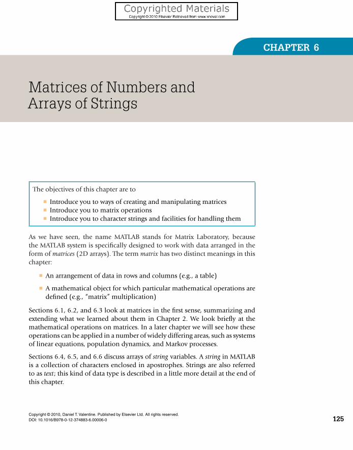
CHAPTER 6
Matrices of Numbers andArrays of Strings
The objectives of this chapter are to
■ Introduce you to ways of creating and manipulating matrices■ Introduce you to matrix operations■ Introduce you to character strings and facilities for handling them
As we have seen, the name MATLAB stands for Matrix Laboratory, becausethe MATLAB system is specifically designed to work with data arranged in theform of matrices (2D arrays). The term matrix has two distinct meanings in thischapter:
■ An arrangement of data in rows and columns (e.g., a table)
■ A mathematical object for which particular mathematical operations aredefined (e.g., “matrix” multiplication)
Sections 6.1, 6.2, and 6.3 look at matrices in the first sense, summarizing andextending what we learned about them in Chapter 2. We look briefly at themathematical operations on matrices. In a later chapter we will see how theseoperations can be applied in a number of widely differing areas, such as systemsof linear equations, population dynamics, and Markov processes.
Sections 6.4, 6.5, and 6.6 discuss arrays of string variables. A string in MATLABis a collection of characters enclosed in apostrophes. Strings are also referredto as text; this kind of data type is described in a little more detail at the end ofthis chapter.
Copyright © 2010, Daniel T. Valentine. Published by Elsevier Ltd. All rights reserved.DOI: 10.1016/B978-0-12-374883-6.00006-0 125

126 CHAPTER 6: Matrices of Numbers and Arrays of Strings
6.1 MATRICES
In this section we examine creating and manipulating matrices of numbers.
6.1.1 A concrete exampleA ready-mix concrete company has three factories (S1, S2, and S3), which mustsupply three building sites (D1, D2, and D3). The costs of transporting a loadof concrete from any factory to any site, in some suitable currency, are given bythe following cost table:
D1 D2 D3
S1 3 12 10S2 17 18 35S3 7 10 24
The factories can supply 4, 12, and 8 loads per day, respectively, and the sitesrequire 10, 9, and 5 loads per day, respectively. The real problem is to find thecheapest way to satisfy the demands at the sites, but we are not considering thathere.
Suppose the factory manager proposes the following transportation scheme(each entry represents the number of loads to be transported along thatparticular route):
D1 D2 D3
S1 4 0 0S2 6 6 0S3 0 3 5
This is called a solution to the transportation problem. The cost table (and thesolution) can be represented by tables C and X, say, where cij is the entry in rowi and column j of the cost table, with a similar convention for X.
To compute the cost of the solution, each entry in the solution table must bemultiplied by the corresponding entry in the cost table. (This operation is not tobe confused with the mathematical operation of matrix multiplication, whichis discussed later.) We therefore want to calculate
3 × 4 + 12 × 0 + · · · + 24 × 5.
To do this calculation in MATLAB, enter C and X as matrices from the commandline, with a semicolon at the end of each row:
C = [3 12 10; 17 18 35; 7 10 24];X = [4 0 0; 6 6 0; 0 3 5];
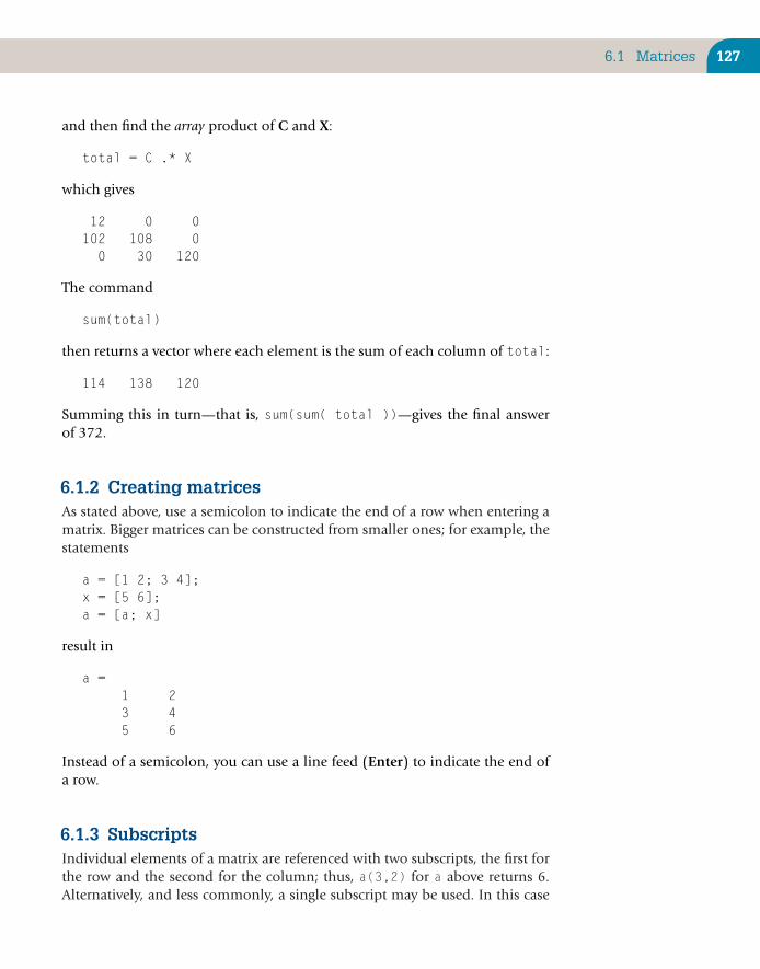
6.1 Matrices 127
and then find the array product of C and X:
total = C .* X
which gives
12 0 0102 108 00 30 120
The command
sum(total)
then returns a vector where each element is the sum of each column of total:
114 138 120
Summing this in turn—that is, sum(sum( total ))—gives the final answerof 372.
6.1.2 Creating matricesAs stated above, use a semicolon to indicate the end of a row when entering amatrix. Bigger matrices can be constructed from smaller ones; for example, thestatements
a = [1 2; 3 4];x = [5 6];a = [a; x]
result in
a =1 23 45 6
Instead of a semicolon, you can use a line feed (Enter) to indicate the end ofa row.
6.1.3 SubscriptsIndividual elements of a matrix are referenced with two subscripts, the first forthe row and the second for the column; thus, a(3,2) for a above returns 6.Alternatively, and less commonly, a single subscript may be used. In this case

128 CHAPTER 6: Matrices of Numbers and Arrays of Strings
you can think of the matrix as being “unwound” column by column, so a(5)for the above example returns 4.
If you refer to a subscript that is out of range (e.g., a(3,3) for a above), youwill get an error message. However, if you assign a value to an element with asubscript that is out of range, the matrix is enlarged to accommodate the newelement. Thus, the assignment
a(3,3) = 7
will add a third column to a with 0s everywhere except at a(3,3).
6.1.4 The transpose operatorThe statements
a = [1:3; 4:6]b = a’
result in
a =1 2 34 5 6
b =1 42 53 6
The transpose operator (’) (apostrophe) turns rows into columns and viceversa.
6.1.5 The colon operatorThe colon operator is extremely powerful and provides very efficient ways ofhandling matrices. For example, if a is the matrix
a =1 2 34 5 67 8 9
the statement
a(2:3,1:2)

6.1 Matrices 129
results in
4 57 8
(i.e., returns the second and third rows, first and second columns). Thestatement
a(3,:)
results in
7 8 9
(i.e., returns the third row). Finally, the statement
a(1:2,2:3) = ones(2)
results in
a =1 1 14 1 17 8 9
(i.e., replaces the 2-by-2 submatrix composed of the first and second row andthe second and third column with a square matrix of 1s).
Essentially, what is happening in the above examples is that the colon operatoris being used to create vector subscripts. However, a colon by itself in place ofa subscript denotes all elements of the corresponding row or column. Thus,a(3,:) means all elements in the third row. This feature may be used, forexample, to construct tables. Suppose we want a table, trig, of the sines andcosines of the angles 0◦ to 180◦ in steps of 30◦. The following statements achievethis:
x = [0:30:180]’;trig(:,1) = x;trig(:,2) = sin(pi/180*x);trig(:,3) = cos(pi/180*x);
You can use vector subscripts to get more complicated effects. For example,
a(:,[1 3]) = b(:,[4 2])
replaces the first and third columns of a by the fourth and second columns ofb (a and b must have the same number of rows).

130 CHAPTER 6: Matrices of Numbers and Arrays of Strings
The colon operator is ideal for the sort of row operations performed in Gaussreduction (a technique of numerical mathematics). For example, if a is thematrix
a =1 –1 22 1 –13 0 1
the statement
a(2,:) = a(2,:) – a(2,1)*a(1,:)
subtracts the first row multiplied by the first element in the second row fromthe second row, resulting in
a =1 –1 20 3 –53 0 1
(the idea being to get a zero immediately underneath a(1,1)).
The keyword end refers to the last row or column of an array. For example, ifr is a row vector, the statement
sum(r(3:end))
returns the sum of all the elements of r from the third one to the last one.
The colon operator may also be used as a single subscript, in which case itbehaves differently if it is on the right-hand or left-hand side of an assignment.On the right-hand side, a(:) gives all the elements of a strung out by columnsin one long column vector. Thus, if
a =1 23 4
the statement
b = a(:)
results in
b =1324

6.1 Matrices 131
However, on the left-hand side of an assignment, a(:) reshapes a matrix. amustalready exist, so a(:) denotes a matrix with the same dimensions (shape) asa but with new contents taken from the right-hand side. In other words, thematrix on the right-hand side is reshaped into the shape of a on the left-handside.
Some examples may help. If
b =1 2 34 5 6
and
a =0 00 00 0
the statement
a(:) = b
results in
a =1 54 32 6
(i.e., the contents of b are strung out into one long column and then fed into aby columns). As another example, the statement
a(:) = 1:6
(with a as above) results in
a =1 42 53 6
Reshaping can also be done with the reshape function. (See Help.)
Whether the colon operator appears on the right- or left-hand side of anassignment, the matrices or submatrices on each side have the same shape.

132 CHAPTER 6: Matrices of Numbers and Arrays of Strings
However, as a special case a single colon subscript may be used to replace allthe elements of a matrix with a scalar:
a(:) = –1
6.1.6 Duplicating rows and columns: TilingSometimes it is useful to generate a matrix where all the rows or columns arethe same. This can be done with the repmat function as follows. If a is the rowvector
a =1 2 3
the statement
repmat(a, [3 1])
results in
ans =1 2 31 2 31 2 3
In Help’s inimitable phraseology, this statement produces a 3-by-1 “tiling” ofcopies of a. You can think of a as a “strip” of three tiles stuck to a self-adhesivebacking. The above statement tiles a floor with three rows and one column ofthis strip.
There is an alternative syntax for repmat:
repmat(a, 3, 1)
An interesting example of this process appears in Section 6.1.15.
6.1.7 Deleting rows and columnsUse the colon operator and the empty array to delete entire rows or columns.For example,
a(:,2) = [ ]
deletes the second column of a. You can’t delete a single element from a matrixwhile keeping it a matrix, so a statement like
a(1,2) = [ ]
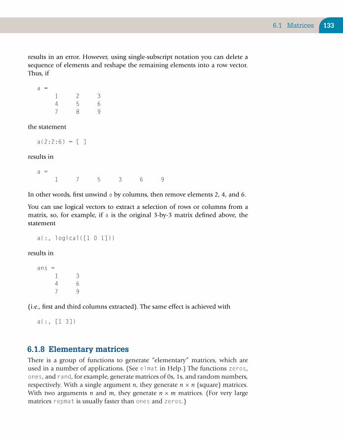
6.1 Matrices 133
results in an error. However, using single-subscript notation you can delete asequence of elements and reshape the remaining elements into a row vector.Thus, if
a =1 2 34 5 67 8 9
the statement
a(2:2:6) = [ ]
results in
a =1 7 5 3 6 9
In other words, first unwind a by columns, then remove elements 2, 4, and 6.
You can use logical vectors to extract a selection of rows or columns from amatrix, so, for example, if a is the original 3-by-3 matrix defined above, thestatement
a(:, logical([1 0 1]))
results in
ans =1 34 67 9
(i.e., first and third columns extracted). The same effect is achieved with
a(:, [1 3])
6.1.8 Elementary matricesThere is a group of functions to generate “elementary” matrices, which areused in a number of applications. (See elmat in Help.) The functions zeros,ones, and rand, for example, generate matrices of 0s, 1s, and random numbers,respectively. With a single argument n, they generate n × n (square) matrices.With two arguments n and m, they generate n × m matrices. (For very largematrices repmat is usually faster than ones and zeros.)

134 CHAPTER 6: Matrices of Numbers and Arrays of Strings
The function eye(n) generates an n × n identity matrix—that is, a matrix with1s on the main “diagonal” and 0s everywhere else. The statement
eye(3)
results in
ans =1 0 00 1 00 0 1
(The original version of MATLAB could not use the more obvious name I forthe identity since it did not distinguish between upper- and lowercase lettersand i was the natural choice for the imaginary unit number.)
As an example, eye may be used to construct a tridiagonal matrix as follows.The statements
a = 2 * eye(5);a(1:4, 2:5) = a(1:4, 2:5) – eye(4);a(2:5, 1:4) = a(2:5, 1:4) – eye(4)
result in
a =2 –1 0 0 0–1 2 –1 0 00 –1 2 –1 00 0 –1 2 –10 0 0 –1 2
Incidentally, if you work with large tridiagonal matrices, you should look at thesparse matrix facilities available in MATLAB via the Help browser.
6.1.9 Specialized matricesThe following functions can be used to generate arbitrary matrices to use ininvestigating matrix operations. These are special matrices discovered by mathe-maticians. You are not expected to understand the motivation for their discoveryor other details about them.
pascal(n) generates a Pascal matrix of order n. Technically, this is a sym-metric positive definite matrix with entries made up from Pascal’striangle. For example,
pascal(4)

6.1 Matrices 135
results in
ans =1 1 1 11 2 3 41 3 6 101 4 10 20
magic(n) generates an n × n magic square.
MATLAB has a number of other functions that generate special matrices, suchas gallery, hadamard, hankel, hilb, toeplitz, and vander. (See elmat inHelp.)
6.1.10 Using MATLAB functions with matricesWhen a MATLAB mathematical or trigonometric function has a matrix argu-ment, it operates on every matrix element, as you would expect. However, manyother MATLAB functions operate on matrices column by column, so if
a =1 0 11 1 10 0 1
the statement
all(a)
results in
ans =0 0 1
For each column of a where all the elements are true (nonzero), all returns 1;otherwise, it returns 0. It therefore returns a logical vector when it takes a matrixargument. To test if all the elements of a are true, use all twice. In this example,the statement
all(all(a))
returns 0 because some of the elements of a are 0. However, the statement
any(a)
returns
ans =1 1 1

136 CHAPTER 6: Matrices of Numbers and Arrays of Strings
because each column of a has at least one nonzero element, and any(any(a))returns 1 since a itself has at least one nonzero element.
If you are not sure whether a particular function operates columnwise orelement by element on matrices, you can always request Help.
6.1.11 Manipulating matricesHere are some functions for manipulating matrices (See Help for details):
■ diag extracts or creates a diagonal.
■ fliplr flips from left to right.
■ flipud flips from top to bottom.
■ rot90 rotates.
■ tril extracts the lower triangular part—for example, the statement
tril(pascal(4))
results in
ans =1 0 0 01 2 0 01 3 6 01 4 10 20
■ triu extracts the upper triangular part.
6.1.12 Array (element-by-element) operationson matrices
All of the array operations discussed in Chapter 2 apply to matrices as well asvectors. For example, if a is a matrix, a * 2 multiplies each of its elements by2, and if
a =1 2 34 5 6
the statement
a .ˆ 2
results in
ans =1 4 916 25 36
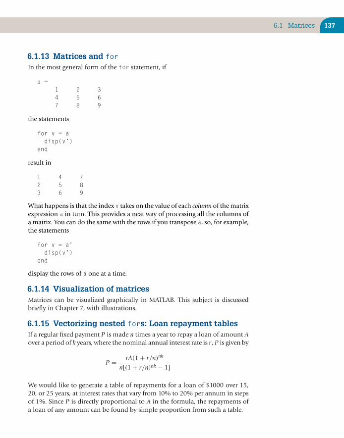
6.1 Matrices 137
6.1.13 Matrices and forIn the most general form of the for statement, if
a =1 2 34 5 67 8 9
the statements
for v = adisp(v’)
end
result in
1 4 72 5 83 6 9
What happens is that the index v takes on the value of each column of the matrixexpression a in turn. This provides a neat way of processing all the columns ofa matrix. You can do the same with the rows if you transpose a, so, for example,the statements
for v = a’disp(v’)
end
display the rows of a one at a time.
6.1.14 Visualization of matricesMatrices can be visualized graphically in MATLAB. This subject is discussedbriefly in Chapter 7, with illustrations.
6.1.15 Vectorizing nested fors: Loan repayment tablesIf a regular fixed payment P is made n times a year to repay a loan of amount Aover a period of k years, where the nominal annual interest rate is r, P is given by
P = rA(1 + r/n)nk
n[(1 + r/n)nk − 1]
We would like to generate a table of repayments for a loan of $1000 over 15,20, or 25 years, at interest rates that vary from 10% to 20% per annum in stepsof 1%. Since P is directly proportional to A in the formula, the repayments ofa loan of any amount can be found by simple proportion from such a table.

138 CHAPTER 6: Matrices of Numbers and Arrays of Strings
The conventional way of handling this is with “nested” fors. The fprintfstatements are necessary to get the output for each interest rate on the sameline (See Section 2.10):
A = 1000; % amount borrowedn = 12; % number of payments per year
for r = 0.1 : 0.01 : 0.2fprintf( ’%4.0f%’, 100 * r );for k = 15 : 5 : 25temp = (1 + r/n) ˆ (n*k);P = r * A * temp / (n * (temp – 1));fprintf( ’%10.2f’, P );
end;fprintf( ’\n’ ); % new line
end;
Here is some sample output (with headings edited in):
rate % 15 yrs 20 yrs 25 yrs
10 10.75 9.65 9.0911 11.37 10.32 9.80...19 16.83 16.21 15.9820 17.56 16.99 16.78
However, we saw in Chapter 2 that for loops can often be vectorized, saving alot of computing time (and also providing an interesting intellectual chal-lenge!). The inner loop can easily be vectorized; the following code uses onlyone for:
...for r = 0.1 : 0.01 : 0.2k = 15 : 5 : 25;temp = (1 + r/n) .ˆ (n*k);P = r * A * temp / n ./ (temp – 1);disp( [100 * r, P] );
end;
Note the use of array operators.
The really tough challenge is to vectorize the outer loop as well. We want a tablewith 11 rows and 3 columns, so we start by assigning values to A and n (fromthe command line):
A = 1000;n = 12;

6.1 Matrices 139
Then we generate a column vector for the interest rates:
r = [0.1:0.01:0.2]’
and change this into a table with 3 columns, each equal to r:
r = repmat(r, [1 3])
The matrix r should look like this:
0.10 0.10 0.100.11 0.11 0.11...0.19 0.19 0.190.20 0.20 0.20
Now we do a similar thing for the repayment periods k. We generate the rowvector
k = 15:5:25
and expand it into a table with 11 rows, each equal to k:
k = repmat(k, [11 1])
This should give us
15 20 2515 20 25...15 20 2515 20 25
The formula for P is a little complicated, so let’s do it in two steps:
temp = (1 + r/n) .ˆ (n * k);P = r * A .* temp / n ./ (temp – 1)
Finally, we should get for P:
10.75 9.65 9.0911.37 10.32 9.80...16.83 16.21 15.9817.56 16.99 16.78
This works because of the way the tables r and k have been constructedand because MATLAB’s array operations are performed element by element.

140 CHAPTER 6: Matrices of Numbers and Arrays of Strings
For example, when the calculation is made for P in row 2 and column 1, thearray operations pick out row 2 of r (all 0.11) and column 1 of k (all 15), givingthe correct value for P (11.37).
The nested for method might be easier to program, but this one is certainlymore interesting (and quicker to execute).
6.1.16 Multidimensional arraysMATLAB arrays can have more than two dimensions. For example, suppose youcreate the matrix
a = [1:2; 3:4]
You can add a third dimension to it with
a(:,:,2) = [5:6; 7:8]
MATLAB responds with
a(:,:,1) =1 23 4
a(:,:,2) =5 67 8
It helps to think of the 3D array a as a series of “pages,” with a matrix oneach one. The third dimension of a numbers the pages. This is analogous to aspreadsheet with multiple sheets, each containing a table (matrix). You can getinto hyperpages with higher dimensions if you like!
See datatypes in Help for a list of special multidimensional array functions.
6.2 MATRIX OPERATIONS
We have seen that array operations are performed element by element on matri-ces. However, matrix operations, which are fundamental to MATLAB, are defineddifferently in certain cases, in the mathematical sense. Addition and subtrac-tion are defined the same as in the equivalent array operations (i.e., element byelement), but multiplication is quite different.
6.2.1 MultiplicationMatrix multiplication is probably the most important matrix operation. It is usedwidely in such areas as network theory linear systems of equations, transfor-mation of coordinate systems, and population modeling, to name but a few.
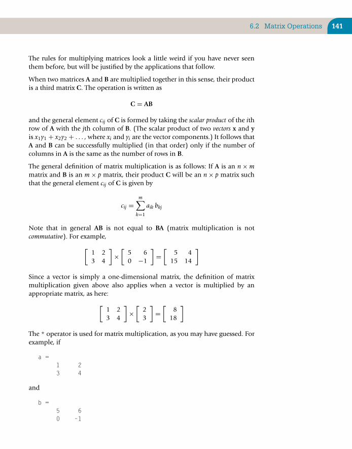
6.2 Matrix Operations 141
The rules for multiplying matrices look a little weird if you have never seenthem before, but will be justified by the applications that follow.
When two matrices A and B are multiplied together in this sense, their productis a third matrix C. The operation is written as
C = AB
and the general element cij of C is formed by taking the scalar product of the ithrow of A with the jth column of B. (The scalar product of two vectors x and yis x1y1 + x2y2 + . . . , where xi and yi are the vector components.) It follows thatA and B can be successfully multiplied (in that order) only if the number ofcolumns in A is the same as the number of rows in B.
The general definition of matrix multiplication is as follows: If A is an n × mmatrix and B is an m × p matrix, their product C will be an n × p matrix suchthat the general element cij of C is given by
cij =m∑
k=1
aik bkj
Note that in general AB is not equal to BA (matrix multiplication is notcommutative). For example,
[1 23 4
]×
[5 60 −1
]=
[5 4
15 14
]
Since a vector is simply a one-dimensional matrix, the definition of matrixmultiplication given above also applies when a vector is multiplied by anappropriate matrix, as here:
[1 23 4
]×
[23
]=
[8
18
]
The * operator is used for matrix multiplication, as you may have guessed. Forexample, if
a =1 23 4
and
b =5 60 –1

142 CHAPTER 6: Matrices of Numbers and Arrays of Strings
the statement
c = a * b
results in
c =5 415 14
Note the important difference between the array operation a .* b (evaluateby hand and check with MATLAB) and the matrix operation a * b.
To multiply a matrix by a vector in that order, the vector must be a columnvector. Thus, if
b = [2 3]’
the statement
c = a * b
results in
c =818
6.2.2 ExponentiationThe matrix operation A2 means A × A, where A must be a square matrix. Theoperator ˆ is used for matrix exponentiation, so, for example, if
a =1 23 4
the statement
a ˆ 2
results in
ans =7 1015 22

6.4 *Strings 143
which is the same as a * a (try it). Again, note the difference between the arrayoperation a .ˆ2 (evaluate by hand and check with MATLAB) and the matrixoperation a ˆ 2.
6.3 OTHER MATRIX FUNCTIONS
Here are some of MATLAB’s more advanced matrix functions.
det determinant.
eig eigenvalue decomposition.
expm matrix exponential (i.e., eA , where A is a matrix). The matrix expo-nential may be used to evaluate analytical solutions of linearordinary differential equations with constant coefficients.
inv inverse.
lu LU factorization (into lower and upper triangular matrices).
qr orthogonal factorization.
svd singular-value decomposition.
6.4 *STRINGS
Strings may be assigned to variables by enclosing them in apostrophes:
s = ’Hi there’;
If an apostrophe is part of the string, it must be repeated:
s = ’o’’clock’;
6.4.1 InputStrings may be entered in response to the input statement in two ways:
■ Enclose the string in apostrophes when you enter it.
■ Use an additional argument ’s’ with input, in which case you mustnot use apostrophes when entering the string:
� name = input( ’Enter your surname: ’, ’s’ );Enter your surname: O’Reilly

144 CHAPTER 6: Matrices of Numbers and Arrays of Strings
6.4.2 Strings as arraysA MATLAB string is actually an array, with each element representing onecharacter. For example, if
s = ’Napoleon’
whos reveals that s is 1 by 8. The statement
s(8:–1:1)
will therefore display the string Napoleon backwards.
If a string must contain an apostrophe, the apostrophe must be repeated whenentering the string. However, only one apostrophe is actually stored in the string.For example, in
name = ’M’’kombe’
name(3) is k.
You can exploit the vector nature of strings in a number of ways. One is to findand/or remove certain characters. The following code will remove all the blanksfrom the string s.
s = ’Twas brillig and the slithy toves’;nonblanks = s ˜= ’ ’;s(nonblanks)
nonblanks is a logical vector with 0s corresponding to the positions of theblanks. Using nonblanks as a subscript removes the blanks. (See Section 5.3.)
6.4.3 String concatenationBecause strings are vectors, they may be concatenated (joined) with squarebrackets:
king = ’Henry’;king = [king, ’ VIII’]
6.4.4 ASCII codes: double and charA MATLAB character is represented internally by a 16-bit numerical value. Thecharacter codes start at 1, and the first 127 are in ASCII format. For example,the ASCII codes for the letters A through Z are the consecutive integers from 65to 90, while the codes for a through z run from 97 to 122. (See Appendix D.)

6.4 *Strings 145
You can see that the ASCII codes for a string with double:
double(’Napoleon’)
return
78 97 112 111 108 101 111 110
Conversely, using char:
char(65:70)
returns a string from the ASCII codes
ABCDEF
You can use char and double to generate rows of identical characters:
x = char(ones(4,20)*double(’#’))
gives
################################################################################
Can you see why? The function ones(4,20) generates 4 rows and 20 columnsof 1s. Multiplying by double(’#’) replaces all the 1s with the ASCII code for# (whatever that is), and char converts the ASCII codes back to text.
If a character variable is involved in an arithmetic expression, MATLAB uses itsASCII code in the calculation. Thus, if
s = ’a’
the expression s + 1 returns 98 since the ASCII code for a is 97.
Array operations can be performed on strings. For example, if s is a string ofletters, the expression char(s+1) returns each letter in the string advanced byone place in the alphabet.
The relationship between characters and their ASCII codes means that you cando interesting things like this:
alpha = double(’a’):double(’z’)
Can you see what the result will be?

146 CHAPTER 6: Matrices of Numbers and Arrays of Strings
6.4.5 String display with fprintfStrings may be displayed with fprintf using the %s format specifier. They canbe right- or left-justified and truncated. The statements
fprintf( ’%8sVIII\n’, ’Henry’ )fprintf( ’%-8sVIII\n’, ’Henry’ )fprintf( ’%.3sVIII\n’, ’Henry’ )
result in
HenryVIIIHenryVIIIHenVIII
To display single characters with fprintf, use the %c format specifier.
6.4.6 Comparing stringsTry out the following statements:
s1 = ’ann’;s2 = ’ban’;s1 < s2
You should get the logical vector
1 0 0
because the logical expression s1 < s2 compares the ASCII codes of the twostrings element by element (the strings must have the same length). This is thebasis of alphabetical sorting.
The function strcmp(s1, s2) compares the two strings s1 and s2, returning1 if they are identical and 0 otherwise. (The strings do not have to be the samelength.)
6.4.7 Other string functionsHere are some additional string-handling functions. See matlab\strfun inHelp for a complete list.
blanks generates a string of blanks.
deblank removes trailing blanks from a string.
int2str, num2str convert their numeric arguments to strings. These func-tions are handy for labeling graphs with text that includesvariable numeric values.
6.5 *Two-Dimensional Strings 147
ischar returns 1 if its argument is a string and 0 otherwise.
lower, upper convert strings to lowercase and uppercase, respectively.
sprintf works like fprintf, except that it returns a stringaccording to the format specification:
s = sprintf( ’Value of K: %g’, K )
returns the string Value of K: 0.015 in s if K has thevalue 0.015.
6.5 *TWO-DIMENSIONAL STRINGS
You can create a two-dimensional character array in the same way you woulda matrix, except that each row must have the same length; if necessary, pad theshorter strings with blanks on the right. For example,
nameAndAddress = [’Adam B Carr ’; ’21 Barkly Ave’;’Discovery ’]
results in
nameAndAddress =
Adam B Carr21 Barkly AveDiscovery
An easier way to create two-dimensional strings is to use the char function,which automatically pads the shorter strings for you:
nameAndAddress = char(’Adam B Carr’, ’21 Barkly Ave’,’Discovery’)
Remember that if you use single-subscript notation, the array is referenced bycolumn. Thus,
nameAndAddress(1:3)
returns
A2D
(the first letter of each row).

148 CHAPTER 6: Matrices of Numbers and Arrays of Strings
6.6 *eval AND TEXT MACROS
If a MATLAB expression is “encoded” as a string in a variable t, say, the functioneval(t) causes it to be evaluated. (Strictly, the string is interpreted.) This is calleda text macro facility. For example, if the following assignment is made:
s = ’x = –b/(2*a);’
eval(s) makes MATLAB interpret the text in s as the statement
x = –b/(2*a);
which is then carried out with the current values of a, b, and c.
Another use of eval is as a “user-friendly” way of inputting a function from theCommand Window. Consider the following script:
f = input( ’Enter function (of x) to be plotted: ’, ’s’ );x = 0:0.01:10;plot(x, eval(f)),grid
Here’s how the command line looks after you enter the function:
� Enter function (of x) to be plotted: exp(–0.5*x) . *sin(x)
Use of the second argument ’s’ for inputmeans that you don’t need to enclosethe text in apostrophes. Whatever expression you enter will be plotted, as longas it is a function of x.
Note that you should use feval (Chapter 10) rather than eval whenever pos-sible, since feval is faster and code using it can be compiled with the MATLABcompiler.
6.6.1 Error trapping with eval and lasterrThe use of eval to evaluate an expression input by a user can misfire if theexpression is invalid—the script grinds to a halt. However, eval together withthe function lasterr enables you to trap and correct errors like this withoutthe script crashing.
The function eval can take a second (string) argument, representing an expres-sion to be executed if an error is encountered in the first argument. This isdemonstrated below with lasterr, which MATLAB sets to the error messagecorresponding to the last error encountered. lasterr can also be set to anystring value. See Help for more details.
As an example, the script below will continue running until you enter a validexpression.

6.6 *eval and Text Macros 149
lasterr(’1’); % true (not empty)while ˜isempty(lasterr)lasterr(’’); % false (empty)f = input( ’Enter expression: ’, ’s’ );f = [f ’;’]; % suppress display when evaluatedeval(f, ’disp(’’Dum-dum!’’)’); % trap error and display messageif ˜isempty(lasterr)lasterrfprintf( ’Please try again!\n’ )
endend
6.6.2 eval with try...catchHahn, the original author of this book (first and second editions) was indebtedto Dean Redelinghuys and Grant Grobbelaar for the following example, whichprovides an alternative way of dealing with errors generated by eval.
The user defines variables in the workspace by typing them in. This input is eval-uated by eval. If an invalid assignment is entered, the script normally crashes.However, if an error occurs in the try clause of a try...catch statement,control is transferred to the catch clause, which deals with it. try...catch isembedded in a while loop, which perseveres until the user eventually enters avalid assignment statement!
stopflag = 0;while ˜stopflag
clc; % Clear the screen!disp(’Your variables are:’)whosa = input(’Enter Variable definition or empty to quit: ’,’s’);if isempty(a),stopflag = 1;
elsetryeval([a ’;’]); % Force no output to command window!
catchdisp(’Invalid variable assignment statement. The error was:’);disp([’ ’, lasterr]);disp(’Press a key to continue’);pause
endend;
end

150 CHAPTER 6: Matrices of Numbers and Arrays of Strings
SUMMARY
■ A matrix is a 2D array. Elements may be referenced in the conventional waywith two subscripts. Alternatively, one subscript may be used, in which casethe matrix is “unwound” by columns.
■ The colon operator may be used to represent all the rows or columns of amatrix; it may also be used as a single subscript.
■ The keyword end refers to the last row or column of a matrix.
■ Use repmat to duplicate rows or columns of a matrix.
■ Use the empty array [ ] to delete rows or columns of a matrix.
■ Arrays may have more than two dimensions. In the case of a 3D array, thethird subscript may be thought of as numbering pages, with each pagecontaining a matrix defined by the first two subscripts.
■ The matrix operations of multiplication and exponentiation areimplemented with the matrix operators * and ˆ.
■ A MATLAB text string is an array in which each element represents onecharacter.
■ Since a string is usually enclosed in apostrophes, if the apostrophe itself isto be included in the string, it must be repeated.
■ Strings may be concatenated (joined) with square brackets.
■ Characters are represented by the numerical ASCII codes: double returnsthe ASCII codes for the characters in a string; char returns the stringrepresented by the ASCII codes in an array.
■ When two strings (of equal length) are compared in a logical expression,their ASCII codes are compared element by element, resulting in a logicalarray.
■ char may be used to create two-dimensional character arrays.
■ eval interprets its string argument as a MATLAB statement. This is the basisfor text macros in MATLAB. eval can be used with lasterr andtry...catch to trap and correct errors.
CHAPTER EXERCISES
6.1. Set up any 3 × 3 matrix a. Write some command-line statements to perform thefollowing operations:

Summary 151
(a) Interchange columns 2 and 3.
(b) Add a fourth column (of 0s).
(c) Insert a row of 1s as the new second row (i.e., move the current second and thirdrows down).
(d) Remove the second column.
6.2. Write a function deblank(s) that removes all blanks from the string s.
6.3. Write a function toupper(s) that translates lowercase letters in the string s touppercase.
6.4. Write a function ispalin(s) that returns 1 if the string s is a palindrome, or 0 if not. Apalindrome is a sentence that reads the same backward as forward, such as Reward aToyota drawer (someone who drawsToyotas,presumably) or Napoleon’s classic lament,Able was I ere I saw Elba. Assume there is no punctuation, remove all the blanks first,and convert all letters to lowercase.
6.5. A formula called Zeller’s congruence may be used to compute the day of the week, giventhe date (within a certain range):
f = 1 + ( [2.6m − 0.2] + k + y + [y/4] + [c/4] − 2c ) modulo 7
where the brackets denote the integer part; modulo 7 means the remainder whendivided by 7; and
■ m is the month number, with January and February taken as months 11 and 12of the preceding year (March is then month 1 and December is month 10).
■ k is the day of the month.■ c is the century.■ y is the year in the century.■ f = 1 is Sunday (f = 2 is Monday, etc.).
For example, 23rd August 1963 is represented by m = 6, k = 23, c = 19, y = 63; 1stJanuary 1800 is represented by m = 11, k = 1, c = 17, y = 99.
Write a function dayofweek(d) that takes the date in the form of a vector d = [ddmm yyyy] (e.g., [9 3 2001] for 9 March 2001) and returns the day of the week (inwords) on which it falls. Test your program on some known dates such as today, yourbirthday, or 7 December 1941 (Pearl Harbor). Hint: use a 2D array of characters for daysof the week.
The formula will not work if you go too far back. Shakespeare and Cervantes both diedon 23 April 1616—Shakespeare, on a Tuesday; Cervantes, on a Saturday! This is becauseEngland had not yet adopted the Gregorian calendar and was consequently ten daysbehind the rest of the world. The formula will also not work if you go too far forward.
(Continued)
6.6. Write a script that will input a number in binary code (e.g., 1100—no blanks between thedigits) and write its decimal value (12 in this case). Hint: Input the number as a string,and make use of the fact that the string is an array.
6.7. Write a function rightfill(s, n) that fills the string s with blanks from the rightuntil its total length is n characters. If s is longer than n characters, it must be truncated.
6.8. Write a function alphacomp(str1, str2) that returns 1 if string str1 is ahead ofstring str2 alphabetically; 0 otherwise. The function should work even if the stringsare not of equal length. If you are feeling energetic, you might like to use alphacompas the basis for sorting a list of words alphabetically.

152 CHAPTER 6: Matrices of Numbers and Arrays of Strings
6.9. Let us examine the information we can obtain about the size of an array or a matrixof numbers. To do this we need to generate a matrix. Let us generate one of randomintegers from 0 to 10 in m rows and n columns (i.e., an m × n matrix of integers between0 and 10). Since the function rand creates random numbers between 0 and 1, weneed to adjust this. We could do it as follows: fix(10*rand(m,n) +1), where mand n must be assigned particular integer values. Generate a 3 × 5 and a 5 × 3 array ofnumbers. Assign them the matrix variable names A and B. Then execute the size(A),length(A), and numel(A) functions to determine the size, the length of the maxi-mum dimension, and the total number of elements in the A matrix. Do the same forthe B matrix. Compare the element halfway between the first and last in the two arrays(i.e., execute the command A(8) == B(8)): Are they the same?
Hint: There are two ways to index the locations in an array. One is by the row andcolumn pair of numbers; the other is by a single index associated with how MATLABcounts the elements in an array. This is done as illustrated in the C matrix given below:
C = [ 1 4 7 10 132 5 8 11 143 6 9 12 15]
In this matrix the numbers in the rows and columns also correspond to the single indexthat identifies their location in the array. The single-index counting procedure is fromtop to bottom in each column, starting from left to right. To verify this try the commandC(10) after you generate this matrix in the command window.
6.10. Generate a 5 × 2 matrix by executing the following command:
A = pi*fix(2*rand(5,2)+1).
Then execute the following command:
round(cos(A)).
Compare your results with your knowledge of the cosine function. Did you get whatyou expected?

CHAPTER 7
Introduction to Graphics
The objective of this chapter is to introduce you to
■ MATLAB’s high-level 2D and 3D plotting facilities.
A picture, it is said, is worth a thousand words. MATLAB has a powerful graphicssystem for presenting and visualizing data that is reasonably easy to use. (Mostof the figures in this book have been generated by MATLAB.) This chapter intro-duces MATLAB’s high-level 2D and 3D plotting facilities. Low-level features,such as handle graphics, are discussed in later sections.
It should be stressed that the treatment in this chapter is of necessity briefand intended only to give you a glimpse of the richness and power of MATLABgraphics. For a full treatment, consult Help on the functions mentioned, as wellas the comprehensive list of graphics functions online: MATLAB: Reference:MATLAB Function Reference: Functions by Category: Graphics.
7.1 BASIC TWO-DIMENSIONAL GRAPHS
Graphs (in 2D) are drawn with the plot statement. In its simplest form, plottakes a single vector argument, as in plot(y). In this case the elements of y areplotted against their indexes. For example, plot(rand(1, 20)) plots 20 ran-dom numbers against the integers 1–20, joining successive points with straightlines, as in Figure 7.1. If y is a matrix, its columns are plotted against elementindexes. Axes are automatically scaled and drawn to include the minimum andmaximum data points.
Copyright © 2010, Daniel T. Valentine. Published by Elsevier Ltd. All rights reserved.DOI: 10.1016/B978-0-12-374883-6.00007-2 153

154 CHAPTER 7: Introduction to Graphics
1
0.8
0.4
0.2
00 5 10 15 20 0
0
1
2
3
1 2 3 4
0.6
(a) (b)
FIGURE 7.1Examples of plot.
Probably the most common form of plot is plot(x, y), where x and y arevectors of the same length:
x = 0:pi/40:4*pi;plot(x, sin(x))
In this case, the coordinates of the ith point are xi, yi. This form of plot wasused widely in earlier chapters.
Straight-line graphs are drawn by giving the x and y coordinates of the endpoints in two vectors. For example, to draw a line between the points withCartesian coordinates (0, 1) and (4, 3), use the statement
plot([0 4], [1 3])
That is, [0 4] contains the x coordinates of the two points, and [1 3] containsthe y coordinates.
MATLAB has a set of easy-to-use plotting commands, all starting with the stringez. The easy-to-use form of plot is ezplot:
ezplot(’tan(x)’)
EXERCISES
1. Draw lines joining the following points: (0, 1), (4, 3), (2, 0), and (5, −2).
2. Draw a “house” similar to the one depicted in Figure 7.1.

7.1 Basic Two-Dimensional Graphs 155
7.1.1 LabelsGraphs may be labeled with the following statements:
gtext(’text’) writes a string (text) in the graph window. It puts acrosshair in the graph window and waits for a mouse button or keyboardkey to be pressed. The crosshair can be positioned with the mouse or thearrow keys. For example,
gtext( ’X marks the spot’ )
Text may also be placed on a graph interactively with Tools → Edit Plot fromthe figure window.
grid adds/removes grid lines to/from the current graph. The grid state maybe toggled.
text(x, y, ’text’) writes text in the graphics window at the point speci-fied by x and y. If x and y are vectors, the text is written at each point. If the textis an indexed list, successive points are labeled with its corresponding rows.
title(’text’) writes the text as a title at the top of the graph.
xlabel(’horizontal’) labels the x-axis.
ylabel(’vertical’) labels the y-axis.
7.1.2 Multiple plots on the same axesThere are at least three ways of drawing multiple plots on the same set of axes(which may however be rescaled if the current data falls outside the range ofthe previous data).
■ Simply to use hold to keep the current plot on the axes. All subsequentplots are added to the axes until hold is released, with either hold offor just hold, which toggles the hold state.
■ Use plot with multiple arguments. For example,
plot(x1, y1, x2, y2, x3, y3, ... )
plots the (vector) pairs (x1, y1), (x2, y2), and so on. The advantage ofthis method is that the vector pairs may have different lengths. MATLABautomatically selects a different color for each pair. If you are plottingtwo graphs on the same axes, you may find plotyy useful—it allowsyou to have independent y-axis labels on the left and the right:
plotyy(x,sin(x), x, 10*cos(x))
(for x suitably defined).

156 CHAPTER 7: Introduction to Graphics
■ Use the form
plot(x, y)
where x and y may both be matrices or where one may be a vector andone a matrix. If one of x or y is a matrix and the other is a vector, therows or columns of the matrix are plotted against the vector, using adifferent color for each. Matrix rows or columns are selected dependingon which have the same number of elements as the vector. If the matrixis square, columns are used. If x and y are both matrices of the samesize, the columns of x are plotted against the columns of y. If x is notspecified, as in plot(y), where y is a matrix, the columns of y areplotted against the row index.
7.1.3 Line styles, markers, and colorLine styles, markers, and color for a graph may be selected with a string argumentto plot. For example,
plot(x, y, ’--’)
joins the plotted points with dashed lines, whereas
plot(x, y, ’o’)
draws circles at the data points with no lines joining them. You can specify allthree properties:
plot(x,sin(x), x, cos(x), ’om--’)
which plots sin(x) in the default style and color and cos(x) with circles joinedby dashes in magenta. The available colors are denoted by the symbols c, m, y,k, r, g, b, w. Have fun trying to figure out what they mean, or use help plotto see the full range of possible symbols.
7.1.4 Axis limitsWhenever you draw a graph, MATLAB automatically scales the axis limits to fitthe data. You can override this with
axis( [xmin, xmax, ymin, ymax] )
which sets the scaling on the current plot. In other words, draw the graph first,then reset the axis limits.
If you want to specify the minimum or maximum of a set of axis limits andhave MATLAB autoscale the other, use Inf or -Inf for the autoscaled limit. Youcan return to the default of automatic axis scaling with

7.1 Basic Two-Dimensional Graphs 157
axis auto
The statement
v = axis
returns the current axis scaling in the vector v. Scaling is frozen at the currentlimits with
axis manual
so that if hold is turned on, subsequent plots will use the same limits.
If you draw a circle, say, with the statements
x = 0:pi/40:2*pi;plot(sin(x), cos(x))
it probably won’t appear round, especially if you resize the figure window.However, the command
axis equal
makes unit increments along the x- and y-axes the same physical length onthe monitor, so that circles always appear round. The effect is undone withaxis normal.
You can turn off axis labeling and tick marks with axis off, and turn them onagain with axis on.
Axes and axis?You and I might be forgiven for thinking that axes denotes the plural of axis,which it indeed does in common English usage. However, in MATLAB axes refersto a particular graphics object, which includes not only the x-axis and y-axis andtheir tick marks and labels but also everything drawn on those particular axes:the actual graphs and any text included in the figure window. Axes objects arediscussed in more detail later in this chapter.
7.1.5 Multiple plots in a figure: subplotYou can show a number of plots in the same figure window with the subplotfunction. It looks a little curious at first, but getting the hang of it is quite easy.The statement
subplot(m,n,p)
divides the figure window into m × n small sets of axes and selects the pth set forthe current plot (numbered by row from the left of the top row). For example,
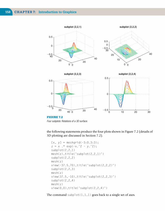
158 CHAPTER 7: Introduction to Graphics
subplot (2,2,1)
020
40
0
20
4020.5
0
0.5
subplot (2,2,2)
0
20
40
0
10
20
3020.5
00.5
subplot (2,2,3)
0 20 40020
40
20.5
0
0.5
subplot (2,2,4)
0 10 20 3020.5
0
0.5
FIGURE 7.2Four subplots: Rotations of a 3D surface.
the following statements produce the four plots shown in Figure 7.2 (details of3D plotting are discussed in Section 7.2).
[x, y] = meshgrid(–3:0.3:3);z = x .* exp(–x.ˆ2 – y.ˆ2);subplot(2,2,1)mesh(z),title(’subplot(2,2,1)’)subplot(2,2,2)mesh(z)view(–37.5,70),title(’subplot(2,2,2)’)subplot(2,2,3)mesh(z)view(37.5,–10),title(’subplot(2,2,3)’)subplot(2,2,4)mesh(z)view(0,0),title(’subplot(2,2,4)’)
The command subplot(1,1,1) goes back to a single set of axes.

7.1 Basic Two-Dimensional Graphs 159
7.1.6 figure, clf, and clafigure(h), where h is an integer, creates a new figure window or makes figureh the current figure. Subsequent plots are drawn in the current figure. h is calledthe figure handle. Handle graphics are discussed further in a later section of thischapter.
clf clears the current figure window. It also resets all properties associated withthe axes, such as the hold state and the axis state. cla deletes all plots andtext from the current axes—that is, it leaves only the x- and y-axes and theirassociated information.
7.1.7 Graphical inputThe command
[x, y] = ginput
allows you to select an unlimited number of points from the current graphusing the mouse or the arrow keys. A movable crosshair appears on the graph.Clicking saves its coordinates in x(i) and y(i). Pressing Enter terminates theinput. An example provided in online Chapter 18 (see Contents section forURL) involves selecting points in a figure and fitting a curve to them.
The command
[x, y] = ginput(n)
works similarly to ginput except that you must select exactly n points. See Helpfor further information.
7.1.8 Logarithmic plotsThe command
semilogy(x, y)
plots y with a log10 scale and x with a linear scale. For example,
x = 0:0.01:4;semilogy(x, exp(x)), grid
produce the graph in Figure 7.3. Equal increments along the y-axis representmultiples of powers of 10, so, starting from the bottom, the grid lines are drawnat 1, 2, 3, . . . , 10, 20, 30 . . . , 100, . . . . Incidentally, the graph of ex on these axesis a straight line because the equation y = ex transforms into a linear equationwhen you take logs of both sides. (See also semilogx and loglog.) Note thatx and y may be vectors and/or matrices, just as in plot.

160 CHAPTER 7: Introduction to Graphics
0 0.5 1 1.5 2 2.5 3 3.5 4100
101
102
FIGURE 7.3Logarithmic plot.
As an exercise, use semilogy to draw graphs of x2, x3, x4, and ex2over the interval
0 ≤ x ≤ 4.
7.1.9 Polar plotsThe point (x, y) in Cartesian coordinates is represented by the point (θ, r) inpolar coordinates, where
x = r cos(θ)
y = r sin(θ)
and θ varies between 0 and 2π radians (360◦).
The command
polar(theta, r)
generates a polar plot of the points, with angles in theta and magnitudes in r.As an example, the statements
x = 0:pi/40:2*pi;polar(x, sin(2*x)),grid
produce the plot shown in Figure 7.4.

7.1 Basic Two-Dimensional Graphs 161
0.2
0.4
0.6
0.8
1
30
210
60
240
90
270
120
300
150
330
180 0
FIGURE 7.4Polar plot of θ against sin(2θ).
7.1.10 Plotting rapidly changing mathematicalfunctions: fplot
In all of the graphing examples so far, the x coordinates of the points plottedhave been incremented uniformly (e.g., x = 0:0.01:4). If the function beingplotted changes very rapidly in some places, this can be inefficient and can evenproduce a misleading graph. As an example, the statements
x = 0.01:0.001:0.1;plot(x, sin(1./x))
produce the graph shown in Figure 7.5(a). If the x increments are reduced to0.0001 however, we get the graph in Figure 7.5(b) instead. For x < 0.04, thetwo graphs look quite different.
MATLAB has a function called fplot that uses a more elegant approach.Whereas the previous method evaluates sin(1/x) at equally spaced intervals,fplot evaluates it more frequently over regions where it changes rapidly. Here’show to use it:
fplot(’sin(1/x)’, [0.01 0.1]) % no, 1./x not needed!

162 CHAPTER 7: Introduction to Graphics
1
0
20.5
210 0.05 0.1
0.5
(a)
1
0
20.5
210 0.05 0.1
0.5
(b)
FIGURE 7.5y = sin(1/x): (a) plot function used, (b) fplot function used.
7.1.11 The Property EditorThe most general way of editing a graph is through the Property Editor: Edit→ Figure Properties from the figure window. This topic is discussed brieflytoward the end of this chapter.
7.2 THREE-DIMENSIONAL PLOTS
MATLAB has a variety of functions for displaying and visualizing data in 3D,either as lines or as various surfaces. This section provides a brief overview.
7.2.1 The plot3 functionThe function plot3 is the 3D version of plot. The command
plot3(x, y, z)
draws a 2D projection of a line in 3D through the points whose coordinatesare the elements of the vectors x, y, and z. As one example,
plot3(rand(1,10), rand(1,10), rand(1,10))
generates 10 random points in 3D space and joins them with lines, as shownin Figure 7.6. As another example,
t = 0:pi/50:10*pi;plot3(exp(–0.02*t).*sin(t), exp(–0.02*t).*cos(t),t), ...xlabel(’x-axis’), ylabel(’y-axis’), zlabel(’z-axis’)

7.2 Three-Dimensional Plots 163
1
0.5
01
0.5
0 00.5
1
40
20
01
0
21210
1
z-a
xis
y -axisx -axis
FIGURE 7.6Two examples of plot3.
produce the inwardly spiraling helix shown in Figure 7.6. Note the orientationof the x-, y-, and z-axes, and that, in particular, the z-axis may be labeled withzlabel.
7.2.2 Animated 3D plots with the comet3 functionThe function comet3 is similar to plot3 except that it draws with a moving“comet head.” Use it to animate the helix in Figure 7.6.
7.2.3 Mesh surfacesIn Chapter 1 we saw how to draw the Mexican hat (Figure 1.3):
[x y ] = meshgrid(–8 : 0.5 : 8);r = sqrt(x.ˆ2 + y.ˆ2) + eps;z = sin(r) ./ r;
This is an example of a mesh surface. To see how such surface is drawn, we take asimpler example, say z = x2 − y2. The surface we are after is the one generatedby the values of z as we move around the x-y plane. Let’s restrict ourselves topart of the first quadrant of this plane, given by
0 ≤ x ≤ 5, 0 ≤ y ≤ 5.
The first step is to set up the grid in the x-y plane over which the surface is to beplotted. We use the MATLAB function meshgrid for this as follows:
[x y] = meshgrid(0:5);
This statement sets up two matrices, x and y. (Functions such as meshgrid,which returns more than one “output argument,” are discussed in detail inChapter 10. However, you don’t need to know the details to use meshgrid here.)

164 CHAPTER 7: Introduction to Graphics
The two matrices in this example are:
x =0 1 2 3 4 50 1 2 3 4 50 1 2 3 4 50 1 2 3 4 50 1 2 3 4 50 1 2 3 4 5
y =0 0 0 0 0 01 1 1 1 1 12 2 2 2 2 23 3 3 3 3 34 4 4 4 4 45 5 5 5 5 5
The effect is that the columns of the matrix x as it is displayed hold thex coordinates of the points in the grid, while the rows of the display of y hold they coordinates. Recalling the way MATLAB array operations are defined, elementby element, this means that the statement
z = x.ˆ2 – y.ˆ2
will correctly generate the surface points:
z =0 1 4 9 16 25–1 0 3 8 15 24–4 –3 0 5 12 21–9 –8 –5 0 7 16–16 –15 –12 –7 0 9–25 –24 –21 –16 –9 0
At the grid point (5, 2), for example, z has the value 52 − 22 = 21. Incidentally,you don’t need to worry about the exact relationship between grid coordinatesand matrix subscripts; this is taken care of by meshgrid.
The statement mesh(z) then plots the surface (Figure 7.7), with mesh linesconnecting the points in the surface that lie above the grid points. Note thatmesh(z) shows the row and column indices (subscripts) of the matrix z on thex- and y-axes. If you want to see proper values, use mesh(x,y,z). This appliesto many of the other 3D plotting functions.
The function mesh draws a surface as a “wire frame.” An alternative visualizationis provided by surf, which generates a faceted view of the surface (in color)—that is, the wire frame is covered with small tiles.
See Help for variations on mesh and surf.

7.2 Three-Dimensional Plots 165
12
34
56
0
2
4
6230
220
210
0
10
20
30
x -axis
y -axis
z-a
xis
FIGURE 7.7Surface z = x2 − y2.
EXERCISES
1. Draw the surface shown in Figure 7.7 with a finer mesh (0.25 units in each direction),
using
[x y] = meshgrid(0:0.25:5);
(the number of mesh points in each direction is 21).
2. The initial heat distribution over a steel plate is given by the function
u(x , y ) = 80y 2e−x2−0.3y 2
Plot the surface u over the grid defined by
−2.1 ≤ x ≤ 2.1, −6 ≤ y ≤ 6
where the grid width is 0.15 in both directions.You should get the plot shown in Figure 7.8.
7.2.4 Contour plotsIf you managed to draw the plot in Figure 7.8, try the command
contour(u)
You should get a contour plot of the heat distribution, as shown in Figure 7.9(a)—that is, its isothermals (lines of equal temperature). Here’s the code:
[x y] = meshgrid(–2.1:0.15:2.1, –6:0.15:6); % x- y-grids differentu = 80 * y.ˆ2 .* exp(–x.ˆ2 – 0.3*y.ˆ2);contour(u)
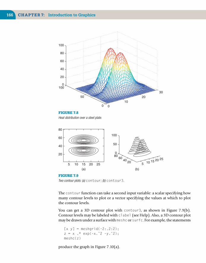
166 CHAPTER 7: Introduction to Graphics
010
20
30
0
50
1000
20
40
60
80
100
FIGURE 7.8Heat distribution over a steel plate.
5
20
40
60
80
10 15
(a) (b)
20 25
800
50
100
6040
20 5 10 15 20 25
FIGURE 7.9Two contour plots: (a) contour; (b) contour3.
The contour function can take a second input variable: a scalar specifying howmany contour levels to plot or a vector specifying the values at which to plotthe contour levels.
You can get a 3D contour plot with contour3, as shown in Figure 7.9(b).Contour levels may be labeled with clabel (see Help). Also, a 3D contour plotmay be drawn under a surface with meshcor surfc. For example, the statements
[x y] = meshgrid(–2:.2:2);z = x .* exp(–x.ˆ2 –y.ˆ2);meshc(z)
produce the graph in Figure 7.10(a).

7.2 Three-Dimensional Plots 167
0.5
0
0 020
4020
4020.5
0.5
0
0 020
4020
4020.5
x -axisy-axis
(a) (b)
FIGURE 7.10(a) meshc; (b) cropping a surface.
7.2.5 Cropping a surface with NaNsIf a matrix for a surface plot contains NaNs, these elements are not plotted,enabling you to cut away (crop) parts of a surface. For example, the statements
[x y] = meshgrid(–2:.2:2, –2:.2:2);z = x .* exp(–x.ˆ2 – y.ˆ2);c = z; % preserve the original surfacec(1:11,1:21) = nan*c(1:11,1:21);mesh(c), xlabel(’x-axis’), ylabel(’y-axis’)
produce the graph in Figure 7.10(b).
7.2.6 Visualizing vector fieldsThe function quiver draws little arrows to indicate a gradient or other vectorfield. Although it produces a 2D plot, quiver is often used in conjunction withcontour, which is why it is described briefly here.
Consider the scalar function of two variables V = x2 + y. The gradient of V isdefined as the vector field
∇V =(
∂V∂x
,∂V∂y
)= (2x, 1)
The following statements draw arrows indicating the direction of ∇V at pointsin the x-y plane (see Figure 7.11):
[x y] = meshgrid(–2:.2:2, –2:.2:2);V = x.ˆ2 + y;dx = 2*x;dy = dx; % dy same size as dxdy(:,:) = 1; % now dy is same size as dx but all 1’scontour(x, y, V), hold onquiver(x, y, dx, dy), hold off

168 CHAPTER 7: Introduction to Graphics
22 21.5 21 20.5 0 0.5 1 1.5 222
21.5
21
20.5
0
0.5
1
1.5
2
FIGURE 7.11Gradients and level surfaces.
The “contour” lines indicate families of level surfaces; the gradient at any point isperpendicular to the level surface that passes through that point. The vectors xand y are needed in the call to contour to specify the axes for the contour plot.
An additional optional argument for quiver specifies the length of the arrows.(See Help.) If you can’t (or don’t want to) differentiate V , you can use thegradient function to estimate the derivative:
[dx dy] = gradient(V, 0.2, 0.2);
The values 0.2 are the increments in the x and y directions used in theapproximation.
7.2.7 Matrix visualizationThe mesh function can also be used to “visualize” a matrix. The followingstatements generate the plot in Figure 7.12:
a = zeros(30,30);a(:,15) = 0.2*ones(30,1);a(7,:) = 0.1*ones(1,30);a(15,15) = 1;mesh(a)

7.2 Three-Dimensional Plots 169
010
20
30
0
10
20
300
0.2
0.4
0.6
0.8
1
FIGURE 7.12Visualization of a matrix.
The matrix a is 30 by 30. The element in the middle, a(15,15), is 1;all the elements in row 7 are 0.1; and all the remaining elements in col-umn 15 are 0.2. mesh(a) interprets the rows and columns of a as anx-y coordinate grid, with the values a(i,j) forming the mesh surface abovethe points (i, j).
The function spy is useful for visualizing sparse matrices.
7.2.8 3D graph rotationThe view function enables you to specify the angle from which you view a3D graph. To see it in operation, run the following program, which rotates thevisualized matrix in Figure 7.12:
a = zeros(30,30);a(:,15) = 0.2*ones(30,1);a(7,:) = 0.1*ones(1,30);a(15,15) = 1;el = 30;for az = –37.5:15:–37.5+360mesh(a), view(az, el)pause(0.5)
end

170 CHAPTER 7: Introduction to Graphics
view takes two arguments. The first one, az in this example, is called the azimuthor polar angle in the x-y plane (in degrees). az rotates the viewpoint (you) aboutthe z-axis—that is, about the “pinnacle” at (15,15) in Figure 7.12—in a counter-clockwise direction. The default value of az is −37.5◦. The program thereforerotates you in a counter-clockwise direction about the z-axis in 15◦ steps startingat the default position.
The second view argument is the vertical elevation el (in degrees). This is theangle that a line from the viewpoint makes with the x-y plane. A value of 90◦for el means you are directly overhead. Positive values of the elevation meanyou are above the x-y plane; negative values mean you are below it. The defaultvalue of el is 30◦.
The command pause(n) suspends execution for n seconds.
You can rotate a 3D figure interactively as follows. Click the Rotate 3D button inthe figure toolbar (first button from the right). Click on the axes, and an outlineof the figure appears to help you visualize the rotation. Drag the mouse in thedirection you want to rotate. When you release the mouse the rotated figure isredrawn.
As an exercise, rewrite the above program to change the elevation gradually,keeping the azimuth fixed at its default.
7.2.9 Other graphics functionsFollowing are more examples of interesting graphics functions. With each,a sample script and graph are shown. You are encouraged to consult thecomplete list of graphics functions in MATLAB FUNCTION REFERENCEonline. Each entry has excellent examples.
Note that the MATLAB function peaks generates a sample surface (see meshzbelow).
For reference purposes the figures are all considered parts of Figure 7.13.Some have been edited with the Edit Tool in the figure window to addcolor.

7.2 Three-Dimensional Plots 171
area
x = 0:0.1:1.5;area(x’, [x.ˆ2’ ...
exp(x)’ exp(x.ˆ2)’])
0 0.5 1 1.50
2
4
6
8
10
12
14
16
18
bar
x = 0:pi/20:pi;bar(x,sin(x))
20.5 0 0.5 1 1.5 2 2.5 3 3.50
0.1
0.2
0.3
0.4
0.5
0.6
0.7
0.8
0.9
1

172 CHAPTER 7: Introduction to Graphics
compass
z = eig(randn(10));compass(z)
1
2
3
30
210
60
240
90
270
120
300
150
330
180 0
errorbar
x = 0:0.1:1;errorbar(x,exp(–x),...
0.5*rand(1,length(x)),’d’)
20.2 0 0.2 0.4 0.6 0.8 1 1.220.2
0
0.2
0.4
0.6
0.8
1
1.2
1.4

7.2 Three-Dimensional Plots 173
ezcontourf
ezcontourf(’xˆ2–yˆ2’)
x
y
26 24 22 0 2 4 626
24
22
0
2
4
6
feather
th = 0:pi/16:pi;z = exp((–0.5+2i)*th);feather(z)
0 2 4 6 8 10 12 14 16 1820.4
20.2
0
0.2
0.4
0.6
0.8
1

174 CHAPTER 7: Introduction to Graphics
fill
t = 0:pi/20:2*pi;fill(cos(t),sin(t),’k’, ...
0.9*cos(t),0.9*sin(t),’y’), ...axis square
21 20.5 0 0.5 121
20.8
20.6
20.4
20.2
0
0.2
0.4
0.6
0.8
1
t = 0:pi/20:4*pi;fill(t,sin(t),’g’)
0 2 4 6 8 10 12 1421
20.8
20.6
20.4
20.2
0
0.2
0.4
0.6
0.8
1
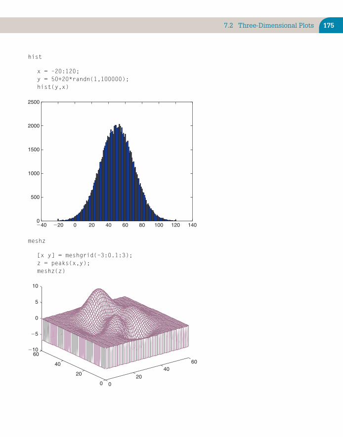
7.2 Three-Dimensional Plots 175
hist
x = –20:120;y = 50+20*randn(1,100000);hist(y,x)
240 220 0 20 40 60 80 100 120 1400
500
1000
1500
2000
2500
meshz
[x y] = meshgrid(–3:0.1:3);z = peaks(x,y);meshz(z)
020
4060
0
20
40
60210
25
0
5
10
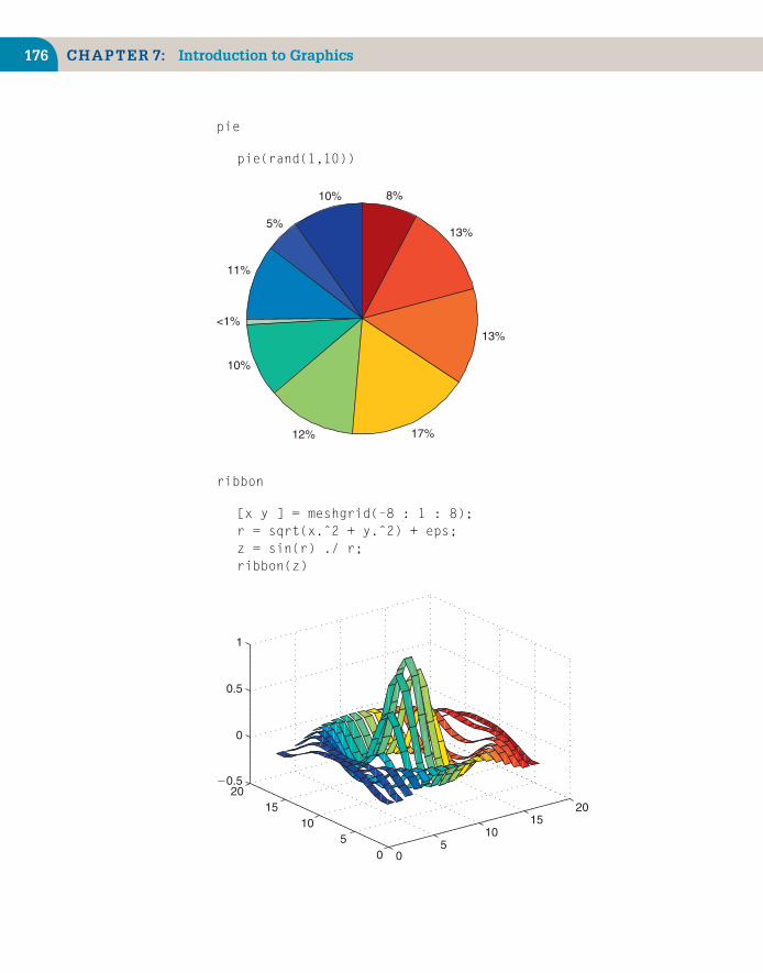
176 CHAPTER 7: Introduction to Graphics
pie
pie(rand(1,10))
10%
5%
11%
<1%
10%
12% 17%
13%
13%
8%
ribbon
[x y ] = meshgrid(–8 : 1 : 8);r = sqrt(x.ˆ2 + y.ˆ2) + eps;z = sin(r) ./ r;ribbon(z)
05
1015
20
05
1015
2020.5
0
0.5
1

7.2 Three-Dimensional Plots 177
t = 0:pi/40:4*pi;y1 = sin(t);y2 = exp(–0.2*t).*sin(2*t);y = [y1; y2];ribbon(t’, y’, 0.1)
0.51
1.52
2.5
0
5
10
1521
20.5
0
0.5
1
stairs
x = 0:pi/40:pi;stairs(x,sin(x))
0 0.5 1 1.5 2 2.5 3 3.50
0.1
0.2
0.3
0.4
0.5
0.6
0.7
0.8
0.9
1

178 CHAPTER 7: Introduction to Graphics
stem3
t = 0:pi/50:2*pi;r = exp(–0.05*t);stem3(r.*sin(t), r.*cos(t),t)
2120.5
00.5
1
21
20.5
0
0.5
10
2
4
6
8
waterfall
[x y] = meshgrid(–2:0.1:2);z = x.*exp(–x.ˆ2–y.ˆ2);waterfall(z)
010
2030
4050
0
20
40
6020.5
0
0.5
SUMMARY
■ 2D plots are drawn with the plot statement.
■ There is a set of easy-to-use plotters called ez*.
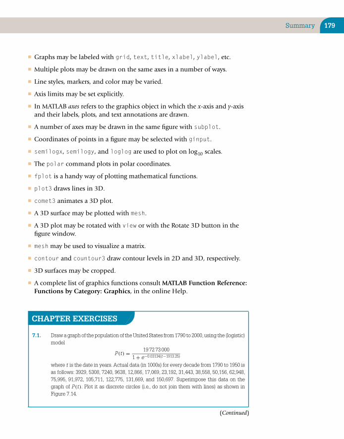
Summary 179
■ Graphs may be labeled with grid, text, title, xlabel, ylabel, etc.
■ Multiple plots may be drawn on the same axes in a number of ways.
■ Line styles, markers, and color may be varied.
■ Axis limits may be set explicitly.
■ In MATLAB axes refers to the graphics object in which the x-axis and y-axisand their labels, plots, and text annotations are drawn.
■ A number of axes may be drawn in the same figure with subplot.
■ Coordinates of points in a figure may be selected with ginput.
■ semilogx, semilogy, and loglog are used to plot on log10 scales.
■ The polar command plots in polar coordinates.
■ fplot is a handy way of plotting mathematical functions.
■ plot3 draws lines in 3D.
■ comet3 animates a 3D plot.
■ A 3D surface may be plotted with mesh.
■ A 3D plot may be rotated with view or with the Rotate 3D button in thefigure window.
■ mesh may be used to visualize a matrix.
■ contour and countour3 draw contour levels in 2D and 3D, respectively.
■ 3D surfaces may be cropped.
■ A complete list of graphics functions consult MATLAB Function Reference:Functions by Category: Graphics, in the online Help.
CHAPTER EXERCISES
7.1. Draw a graph of the population of the United States from 1790 to 2000,using the (logistic)model
P (t) = 19 72 73 0001 + e−0.03134(t−1913.25)
where t is the date in years. Actual data (in 1000s) for every decade from 1790 to 1950 isas follows: 3929, 5308, 7240, 9638, 12,866, 17,069, 23,192, 31,443, 38,558, 50,156, 62,948,75,995, 91,972, 105,711, 122,775, 131,669, and 150,697. Superimpose this data on thegraph of P (t). Plot it as discrete circles (i.e., do not join them with lines) as shown inFigure 7.14.
(Continued)
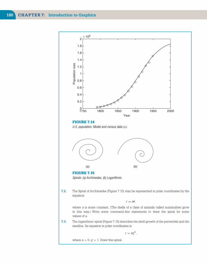
180 CHAPTER 7: Introduction to Graphics
1750
Pop
ulat
ion
size
1800 1850 1900Year
1950 20000
0.2
0.4
0.6
0.8
1
1.2
1.4
1.6
1.8
23108
FIGURE 7.14U.S. population: Model and census data (◦).
(a) (b)
FIGURE 7.15Spirals: (a) Archimedes, (b) Logarithmic.
7.2. The Spiral of Archimedes (Figure 7.15) may be represented in polar coordinates by theequation
r = aθ,
where a is some constant. (The shells of a class of animals called nummulites growin this way.) Write some command-line statements to draw the spiral for somevalues of a.
7.3. The logarithmic spiral (Figure 7.15) describes the shell growth of the periwinkle and thenautilus. Its equation in polar coordinates is
r = aq θ ,
where a > 0, q > 1. Draw this spiral.

Summary 181
FIGURE 7.16A perfect sunflower?
7.4. The arrangement of seeds in a sunflower head (and flowers such as daisies) follows afixed mathematical pattern. The nth seed is at position
r = √n,
with angular coordinate πdn/180 radians, where d is the constant angle of divergence(in degrees) between any two successive seeds (i.e., between the seeds n and (n + 1).Aperfect sunflower head (Figure 7.16) is generated by d = 137.51◦.Write a program to plotthe seed’s pattern, using a circle (o) for each seed. A remarkable feature of this modelis that the angle d must be exact to get proper sunflowers. Experiment with differentvalues, such as 137.45◦ (spokes, from fairly far out), 137.65◦ (spokes all the way), and137.92◦ (Catherine wheels).
7.5. The equation of an ellipse in polar coordinates is given by
r = a(1 − e2)/(1 − e cos θ),
where a is the semi-major axis and e is the eccentricity, if one focus is at the origin andthe semi-major axis lies on the x -axis.
(Continued)
Halley’s Comet, which visited us in 1985/1986, moves in an elliptical orbit about the Sun(at one focus) with a semi-major axis of 17.9 A.U. (astronomical unit, the mean distanceof the Earth from the Sun, which is 149.6 million km). The eccentricity of the orbit is

182 CHAPTER 7: Introduction to Graphics
0.967276. Write a program that draws the orbit of Halley’s Comet and the Earth (assumethe Earth is circular).
7.6. A very interesting iterative relationship much studied recently is defined by
yk+1 = ryk (1 − yk )
(this is a discrete form of the well-known logistic model ). Given y0 and r , successive yk ’smay be easily computed. For example, if y0 = 0.2 and r = 1, then y1 = 0.16, y2 = 0.1334,and so on.This formula is often used to model population growth in cases where growthis limited, restricted by shortages of food, living area, and the like.
yk exhibits fascinating behavior, known as mathematical chaos , for values of r between3 and 4 (independent of y0).Write a program that plots yk against k (as individual points).
Values of r that give particularly interesting graphs are 3.3, 3.5, 3.5668, 3.575, 3.5766,3.738, 3.8287, and many more that can be found by patient exploration.
7.7. A rather beautiful fractal picture can be drawn by plotting the points (xk , yk ) generatedby the following difference equations
xk+1 = yk (1 + sin 0.7xk ) − 1.2√|xk |,
yk+1 = 0.21 − xk ,
starting with x0 = y0 = 0. Write a program to draw the picture (plot individual points;do not join them).
7.8. The following script takes advantage of MATLAB’s ability to deal with complex numbers.It implements the Joukowski transformation of aerodynamics used to conformally mapa circle to an airfoil. Such a mapping is used to map the flow field as well and hencedetermine the flow field around an airfoil, knowing the flow field around a circle inideal flow.
% This is a Joukowski airfoil MATLAB code% that conformally maps a circle to an airfoil% by Daniel T. Valentine .... April 2009% Notes:% The circle is in the (xp,yp) complex plane.% The transform from (xp,yp) to (x,y) is:% x = (xp – e), y = yp% The complex variables of interest are:% zp = xp + i*yp% z = x + i*y% w = u + i*v% Parameter –a is the angle of attack:
a = –5; % in degreesa = a*pi/180; % Conversion to radians
% Parameter related to thickness of the airfoil:e = 0.1;
% Parmeter related to camber of the airfoil:f = 0.1;
% Coordinates of Circle of radius

Summary 183
% R > 1 in zp-planeR = 1 + e;
theta = 0:pi/200:2*pi;yp = R * sin(theta);xp = R * cos(theta);
% plot of circleplot(xp,yp)
hold on% Transformation circle from zp-plane to z-plane:
z = (xp – e) + i.*(yp + f);% Joukowski transformation: z-plane to w-plane
rot = exp(i*a);w = 0.5 .* rot .* (z + 1./z);
% Plot of airfoil in w-planeplot(real(w),imag(w),’r’), axis image
CHAPTER 8
Loops
The objectives of this chapter are to enable you to
■ Program (or code) determinate loops with for.■ Program (or code) indeterminate loops with while.
In Chapter 2 we introduced the powerful for statement, which is used to repeata block of statements a fixed number of times. This type of structure, where thenumber of repetitions must be determined in advance, is sometimes calleddeterminate repetition. However, it often happens that the condition to end aloop is only satisfied during the execution of the loop itself . Such a structure iscalled indeterminate. We begin with a discussion of determinate repetition.
8.1 DETERMINATE REPETITION WITH for
In this section several applications of determinate loops are described.
8.1.1 Binomial coefficientThe binomial coefficient is widely used in mathematics and statistics. It is definedas the number of ways of choosing r objects out of n without regard to orderand is given by
(nr
)= n!
r!(n − r)! (8.1)
Copyright © 2010, Daniel T. Valentine. Published by Elsevier Ltd. All rights reserved.DOI: 10.1016/B978-0-12-374883-6.00008-4 185

186 CHAPTER 8: Loops
If this form is used, the factorials can get very big, causing an overflow. But alittle thought reveals that we can simplify Equation (8.1) as follows:
(nr
)= n(n − 1)(n − 2) · · · (n − r + 1)
r! (8.2)
e.g.,(
103
)= 10!
3! × 7! = 10 × 9 × 81 × 2 × 3
Equation (8.2) is computationally much more efficient:
ncr = 1;n = ...r = ...
for k = 1:rncr = ncr * (n – k + 1) / k;
end
disp( ncr )
The binomial coefficient is sometimes referred to as “n-see-r.” Work throughthe program by hand with some sample values.
8.1.2 Update processesMany problems in science and engineering involve modeling a process wherethe main variable is repeatedly updated over a period of time. Here is an exampleof such an update process.
A can of orange juice at temperature 25◦ C is placed in a refrigerator where theambient temperature F is 10◦ C. We want to find out how the temperature ofthe orange juice changes over a period of time. A standard way of approachingthis type of problem is to break the time period into a number of small steps,each of length dt. If Ti is the temperature at the beginning of step i, we can usethe following model to get Ti+1 from Ti:
Ti+1 = Ti − K dt (Ti − F) (8.3)
where K is a constant parameter depending on the insulating properties of thecan and the thermal properties of the juice. Assume that units are chosen sothat time is in minutes.
The following script implements this scheme. To make the solution more gen-eral, take the starting time as a and the end time as b. If dt is very small, it willbe inconvenient to have output displayed after every step, so the script also

8.1 Determinate Repetition with for 187
asks you for the output interval, opint. This is the time (in minutes) betweensuccessive rows of output. It checks that this interval is an integer multipleof dt. Try the script with some sample values, say dt = 0.2 minutes andopint = 5 minutes (these are the values used for the output below).
K = 0.05;F = 10;a = 0; % start timeb = 100; % end timetime = a; % initialize timeT = 25; % initialize temperatureload train % prepare to blow the whistledt = input( ’dt: ’ );opint = input( ’output interval (minutes): ’ );if opint/dt ˜= fix(opint/dt)sound(y, Fs) % blow the whistle!disp( ’output interval is not a multiple of dt!’ );break
end
clcformat bankdisp( ’ Time Temperature’ );disp( [time T] ) % display initial values
for time = a+dt : dt : bT = T – K * dt * (T – F);if abs(rem(time, opint)) < 1e–6 % practically zero!disp( [time T] )
endend
The output is
Time Temperature0 25.00
5.00 21.67...
95.00 10.13100.00 10.10
Note the following:
■ The function rem is used to display the results every opint minutes:When time is an integer multiple of opint, its remainder when dividedby opint should be zero. However, due to rounding error, the

188 CHAPTER 8: Loops
remainder is not always exactly zero. It is therefore better to test whetherits absolute value is less than some very small value. (Rounding error isdiscussed in Chapter 9.)
■ While this is probably the most obvious way of writing the script, wecannot easily plot the graph of temperature against time this way, sincetime and T are scalars that are repeatedly updated. They both need to bevectors for the graph to be plotted (see Chapter 11).
■ Note how sound is implemented. See help audio for other interestingsounds supplied by MATLAB.
■ In case you are wondering how I got the headings in the right place, I’lllet you in on the secret. Run the script without a heading but with thenumerical output as you want it. Then simply paste the disp statementwith the headings into the Command Window and edit it until theheadings fall in the right place. Paste the final version of disp into thescript.
■ Note the use of break to stop the script prematurely if the user gives badinput. See below for more general use of break.
8.1.3 Nested forsAs we saw in Section 6.1.15, for loops can be nested inside each other. Themain point to note is that the index of the inner for moves faster.
8.2 INDETERMINATE REPETITION WITH while
Determinate loops all have in common the fact that you can work out in prin-ciple exactly how many repetitions are required before the loop starts. In the nextexample, however, there is no way in principle to work out the number of repeats,so a different structure is needed.
8.2.1 A guessing gameThe problem is easy to state. MATLAB “thinks” of an integer between 1 and10 (i.e., it generates one at random). You have to guess it. If your guess is toohigh or too low, the script must say so. If your guess is correct, a message ofcongratulations must be displayed.
A little more thought is required here, so a structure plan might be helpful:
1. Generate random integer2. Ask user for guess

8.2 Indeterminate Repetition with while 189
3. While guess is wrong:If guess is too low
Tell her it is too lowOtherwise
Tell her it is too highAsk user for new guess
4. Polite congratulations5. Stop
Here is the script:
matnum = floor(10 * rand + 1);guess = input( ’Your guess please: ’ );load splat
while guess ˜= matnumsound(y, Fs)
if guess > matnumdisp( ’Too high’ )
elsedisp( ’Too low’ )
end;
guess = input( ’Your next guess please: ’ );end
disp( ’At last!’ )load handelsound(y, Fs) % hallelujah!
Try it out a few times. Note that the while loop repeats as long as matnumis not equal to guess. There is no way in principle of knowing how manyloops will be needed before the user guesses correctly. The problem is trulyindeterminate.
Note that guess has to be input twice: first to get the while loop going andthen during its execution.
8.2.2 The while statementIn general the while statement looks like this:
while conditionstatements
end

190 CHAPTER 8: Loops
while repeats statements WHILE its condition remains true. The condition is there-fore the one to repeat and is tested each time BEFORE statements are repeated. Forthis reason, it is possible to arrange for statements not to be executed at all undercertain circumstances. Clearly, condition must depend on statements in some way;otherwise, the loop will never end.
Recall that a vector condition is considered true only if all its elements arenonzero.
The command-line form of while is
while condition statements, end
8.2.3 Doubling time of an investmentSuppose we have invested some money that draws 10% interest per year, com-pounded. We want to know how long it will take for the investment to double.More specifically, we want a statement of the account each year until the bal-ance has doubled. The English statement of the problem hints heavily that weshould use an indeterminate loop with the following structure plan:
1. Initialize balance, year, interest rate2. Display headings3. Repeat
Update balance according to interest rateDisplay year, balance
until balance exceeds twice original balance4. Stop
A program to implement this plan is
a = 1000;r = 0.1;bal = a;year = 0;disp( ’Year Balance’ )
while bal < 2 * abal = bal + r * bal;year = year + 1;disp( [year bal] )
end
Note that the more natural phrase in the structure plan “until balance exceedstwice original balance” must be coded as
while bal < 2 * a ...

8.2 Indeterminate Repetition with while 191
This condition is checked each time before another loop is made. Repetitionoccurs only if the condition is true. Here’s some output (for an opening balanceof $1000):
Year Balance
1 1100.002 1210.003 1331.004 1464.105 1610.516 1771.567 1948.728 2143.59
When the last loop has been completed, the condition to repeat is false forthe first time, since the new balance ($2143.59) is more than $2000. Also, adeterminate for loop cannot be used here because we don’t know how manyloops are going to be needed until after the script has run (although, in thisparticular example, perhaps you could work out in advance how many repeatsare needed).
If you want to write the new balance only while it is less than $2000, all thathas to be done is to move the statement
disp( [year bal] )
until it is the first statement in the while loop. The initial balance of $1000 isnow displayed.
8.2.4 Prime numbersMany people are obsessed with prime numbers, and most books on program-ming have to include an algorithm to test if a given number is prime. Here’smine.
A number is prime if it is not an exact multiple of any other number except itselfand 1—that is, if it has no factors except itself and 1. The easiest plan of attackis as follows. Suppose P is the number to be tested. See if any numbers N canbe found that divide into P without remainder. If there are none, P is prime.Which numbers N should we try? We can speed things up by restricting P toodd numbers so we only have to try odd divisors N. When do we stop testing?When N = P? No, we can stop a lot sooner. In fact, we can stop once N reaches√
P, since if there is a factor greater than√
P there must be a correspondingfactor less than
√P, which we have found. And where do we start? Well, since

192 CHAPTER 8: Loops
N = 1 will be a factor of any P, we should start at N = 3. The structure plan isas follows:
1. Input P2. Initialize N to 33. Find remainder R when P is divided by N4. While R �= 0 and N <
√P repeat:
Increase N by 2Find R when P is divided by N
5. If = R �= 0 thenP is prime
ElseP is not prime
6. Stop
Note that there may be no repeats—that is, R might be zero the first time. Notealso that there are two conditions under which the loop may stop. Consequently,an if is required after completion of the loop to determine which conditionstopped it.
See if you can write the script. Then try it out on the following numbers:4,058,879 (not prime), and 2,147,483,647 (prime). If such things interest you,the largest known prime number at the time of writing was 26972593 − 1 (discov-ered in June 1999). It has 2,098,960 digits and would occupy about 70 pagesif printed in a newspaper. Obviously, our algorithm cannot test such a largenumber since it is unimaginably greater than the largest number that can berepresented by MATLAB.
8.2.5 Projectile trajectoryIn Chapter 3 we considered the flight of a projectile, given the usual equationsof motion (assuming no air resistance). We would now like to know whenand where it will hit the ground. Although this problem can be solved witha determinate loop (if you know enough applied mathematics), it is also ofinterest to see how to solve it with an indeterminate while loop. The ideais to calculate the trajectory repeatedly with increasing time while the verticaldisplacement (y) remains positive. Here’s the script:
dt = 0.1;g = 9.8;u = 60;ang = input( ’Launch angle in degrees: ’ );ang = ang * pi / 180; % convert to radiansx = 0; y = 0; t = 0; % for startersmore(15)

8.2 Indeterminate Repetition with while 193
while y >= 0disp( [t x y] );t = t + dt;y = u * sin(ang) * t - g * tˆ2 / 2;x = u * cos(ang) * t;
end
The command more(n) gives you n lines of output before pausing. This is calledpaging. To get another single line of output, press Enter. To get the next page ofn lines, press the spacebar. To quit the script, press q.
Try the script for different launch angles. Can you find the angle that gives themaximum horizontal range (x)? What angle keeps it in the air for the longesttime?
Note that when the loop finally ends, the value of y will be negative (check thisby displaying y). However, the position of the disp statement ensures that onlypositive values of y are displayed. If for some reason you need to record the lastvalue of t, say, before y becomes negative, you will need an if statement insidethe while:
if y >= 0tmax = t;
end
Change the script so that it displays the last time for which ywas positive (tmax)after the while loop has ended.
Now suppose we want to plot the trajectory, as shown in Figure 8.1. Note inparticular how the trajectory stops above the x-axis. We need to use vectors now.Here is the script:
dt = 0.1;g = 9.8;u = 60;ang = input( ’Launch angle in degrees: ’ );ang = ang * pi / 180; % convert to radiansxp = zeros(1); yp = zeros(1); % initializey = 0; t = 0;i = 1; % initial vector subscript
while y >= 0t = t + dt;i = i + 1;y = u * sin(ang) * t – g * tˆ2 / 2;
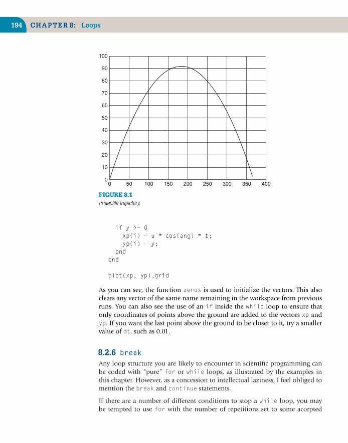
194 CHAPTER 8: Loops
00
10
20
30
40
50
60
70
80
90
100
50 100 150 200 250 300 350 400
FIGURE 8.1Projectile trajectory.
if y >= 0xp(i) = u * cos(ang) * t;yp(i) = y;
endend
plot(xp, yp),grid
As you can see, the function zeros is used to initialize the vectors. This alsoclears any vector of the same name remaining in the workspace from previousruns. You can also see the use of an if inside the while loop to ensure thatonly coordinates of points above the ground are added to the vectors xp andyp. If you want the last point above the ground to be closer to it, try a smallervalue of dt, such as 0.01.
8.2.6 breakAny loop structure you are likely to encounter in scientific programming canbe coded with “pure” for or while loops, as illustrated by the examples inthis chapter. However, as a concession to intellectual laziness, I feel obliged tomention the break and continue statements.
If there are a number of different conditions to stop a while loop, you maybe tempted to use for with the number of repetitions set to some accepted
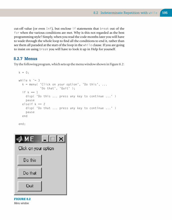
8.2 Indeterminate Repetition with while 195
cut-off value (or even Inf), but enclose if statements that break out of thefor when the various conditions are met. Why is this not regarded as the bestprogramming style? Simply, when you read the code months later you will haveto wade through the whole loop to find all the conditions to end it, rather thansee them all paraded at the start of the loop in the while clause. If you are goingto insist on using break you will have to look it up in Help for yourself.
8.2.7 MenusTry the following program, which sets up the menu window shown in Figure 8.2:
k = 0;
while k ˜= 3k = menu( ’Click on your option’, ’Do this’, ...
’Do that’, ’Quit’ );if k == 1disp( ’Do this ... press any key to continue ...’ )pause
elseif k == 2disp( ’Do that ... press any key to continue ...’ )pause
end
end;
FIGURE 8.2Menu window.

196 CHAPTER 8: Loops
Note that
■ The menu function enables you to set up a menu of user choices.
■ menu takes only string arguments. The first one is the menu title. Thesecond and subsequent strings are the choices available to the user.
■ The value returned by menu (k here) numbers the user’s choices.
■ Since you have no idea how many choices the user will make, menuis properly enclosed in an indeterminate while loop. The loopcontinues to present the menu until the last option (in this example)is selected.
■ You can design much more sophisticated menu-driven applicationswith the MATLAB GUIDE (Graphical User Interface DevelopmentEnvironment).
SUMMARY
■ A for statement should be used to program a determinate loop, where thenumber of repeats is known (in principle) before the loop is encountered.This situation is characterized by the general structure plan:
Repeat N times:Block of statements to be repeated
where N is known or computed before the loop is encountered for the firsttime, and is not changed by the block.
■ A while statement should be used to program an indeterminate repeatstructure, where the exact number of repeats is not known in advance.Another way of saying this is that these statements should be used wheneverthe truth value of the condition for repeating is changed in the body of theloop. This situation is characterized by the following structure plan:
While condition is true repeat:statements to be repeated (reset truth value of condition)
condition is the condition to repeat.
■ In some situations, the statements in a while construct may never beexecuted.
■ Loops may be nested to any depth.
■ The menu statement inside a while loop may be used to create a menu ofuser choices.
Summary 197
CHAPTER EXERCISES
8.1. A person deposits $1000 in a bank. Interest is compounded monthly at the rate of1% per month. Write a program that will compute the monthly balance, but only onan annual basis, for 10 years (use nested for loops, with the outer loop for 10 yearsand the inner loop for 12 months). Note that after 10 years the balance is $3300.39,whereas if interest had been compounded annually at the rate of 12% per year thebalance would only have been $3105.85. See if you can vectorize your solution.
8.2. There are many formulae for computing π (the ratio of a circle’s circumference to itsdiameter). The simplest is
π
4= 1 − 1/3 + 1/5 − 1/7 + 1/9 − · · · (8.4)
which comes from putting x = 1 in the series
arctan x = x − x 3
3+ x 5
5− x 7
7+ x 9
9− · · · (8.5)
(a) Write a program to compute π using Equation (8.4). Use as many terms in theseries as your computer will reasonably allow (start modestly, with 100 terms,say,and rerun your program with more and more each time).You should find thatthe series converges very slowly—it takes a lot of terms to get fairly close to π.
(b) Rearranging the series speeds up the convergence:
π
8= 1
1 × 3+ 1
5 × 7+ 1
9 × 11· · ·
Write a program to compute π using this series instead. You should find thatyou need fewer terms to reach the same level of accuracy that you got in (a).
(c) One of the fastest series for π is
π
4= 6 arctan
18
+ 2 arctan157
+ arctan1
239
Use this formula to compute π. Don’t use the MATLAB function atan to com-pute the arctangents, since that would be cheating. Use Equation (8.5) instead.
(d) Can you vectorize any of your solutions (if you haven’t already)?
(Continued)
8.3. The following method of computing π was discovered by Archimedes:
1. Let A = 1 and N = 62. Repeat 10 times, say:
Replace N by 2NReplace A by [2 − √
(4 − A2)]1/2
Let L = NA/2Let U = L/
√1 − A2/2
Let P = (U + L)/2 (estimate of π)Let E = (U − L)/2 (estimate of error)Print N , P , E
3. Stop
Write a program to implement the algorithm.

198 CHAPTER 8: Loops
8.4. Write a program to compute a table of the function
f (x ) = x sin[
π(1 + 20x )2
]
over the (closed) interval [−1, 1] using increments in x of (a) 0.2, (b) 0.1, and (c) 0.01.
Use your tables to sketch graphs of f (x ) for the three cases (by hand), and observe thatthe tables for (a) and (b) give the wrong picture of f (x ). Have your program draw thegraph of f (x ) for the three cases, superimposed.
8.5. The transcendental number e (2.71828182845904 …) can be shown to be the limit of
(1 + x )1/x
as x tends to zero (from above). Write a program that shows how this expressionconverges to e as x gets closer and closer to zero.
8.6. A square wave of period T may be defined by the function
f (t ) ={
1 (0 < t < T )−1 ( − T < t < 0).
The Fourier series for f (t ) is given by
F (t ) = 4π
∞∑k=0
12k + 1
sin[
(2k + 1)πtT
]
It is of interest to know how many terms are needed for a good approximation of thisinfinite sum. Taking T = 1, write a program to compute and plot to n terms the sumof the series for t from −1.1 to 1.1 in steps of, say, 0.01. Run the program for differentvalues of n.
Superimpose plots of F (t ) against t for a few values of n.
On each side of a discontinuity a Fourier series exhibits peculiar oscillatory behaviorknown as the Gibbs phenomenon. Figure 8.3 shows this clearly for the above serieswith n = 20 (and increments in t of 0.01). The phenomenon is much sharper forn = 200 and t increments of 0.001.
8.7. If an amount of money A is invested for k years at a nominal annual interest rater (expressed as a decimal fraction), the value V of the investment after k years isgiven by
V = A(1 + r/n)nk
where n is the number of compounding periods per year. Write a program to computeV as n gets larger and larger—that is, as the compounding periods become more andmore frequent: monthly, daily, hourly, and so forth. Take A = 1000, r = 4%, and k = 10years. You should observe that your output gradually approaches a limit. Hint : use afor loop that doubles n each time, starting with n = 1.
Compute the value of the formula Aerk for the same values of A, r , and k (use theMATLAB function exp), and compare it with the values of V computed above. Whatdo you conclude?

Summary 199
21.5 21 20.5 0 0.5 1 1.521.5
21
20.5
0
0.5
1
1.5
FIGURE 8.3Fourier series: The Gibbs phenomenon.
8.8. Write a program to compute the sum of the series 12 + 22 + 32 . . . such that the sum isas large as possible without exceeding 1000. The program should display how manyterms the sum uses.
8.9. One of the programs in Section 8.2 shows that an amount of $1000 will double in eightyears with an interest rate of 10%. Using the same interest rate, run the program withinitial balances of $500, $2000, and $10,000 (say) to see how long they take to double.The results may surprise you.
8.10. Write a program to implement the structure plan of Exercise 3.2.
8.11. Use the Taylor series
cos x = 1 − x 2
2! + x 4
4! − x 6
6! + · · ·
to write a program to compute cos x correct to four decimal places (x is in radians).See how many terms are needed to get 4-figure agreement with the MATLAB functioncos. Don’t make x too large; that could cause rounding error.
(Continued)
8.12. A student borrows $10,000 to buy a used car. Interest on her loan is compounded atthe rate of 2% per month while the outstanding balance is more than $5000; at 1% permonth otherwise. She pays back $300 every month except for the last month, when therepayment must be less than $300. She pays at the end of the month, after the intereston the balance has been compounded.The first repayment is made one month after theloan is paid out.Write a program that displays a monthly statement of the balance (afterthe monthly payment has been made), the final payment, and the month of the finalpayment.

200 CHAPTER 8: Loops
8.13. When a resistor (R), capacitor (C ), and battery (V ) are connected in series, a charge Qbuilds up on the capacitor according to the formula
Q(t ) = CV(1 − e−t/RC )
if there is no charge on the capacitor at time t = 0. The problem is to monitor thecharge on the capacitor every 0.1 seconds in order to detect when it reaches a level of8 units of charge, given that V = 9, R = 4, and C = 1. Write a program that displaysthe time and charge every 0.1 seconds until the charge first exceeds 8 units (i.e., thelast charge displayed must exceed 8). Once you have done this, rewrite the programto display the charge only while it is less than 8 units.
8.14. Adapt your program for the prime number algorithm in Section 8.2 to find all the primefactors of a given number (even or odd).

CHAPTER 9
Errors and Pitfalls
The objective of this chapter is to enable you to
■ Recognize and avoid common errors and pitfalls.
Even experienced programmers seldom have programs run correctly the firsttime. In computer jargon, an error in a program is a bug. The story is thata hapless moth short-circuited two thermionic valves in one of the earliestcomputers. This primeval (charcoaled) “bug” took days to find. The process ofdetecting and correcting errors is therefore called debugging.
There are many types of errors and pitfalls, some that are peculiar to MATLABand some that may occur when programming in any language. These arediscussed briefly in this chapter.
9.1 SYNTAX ERRORS
Syntax errors are typing mistakes in MATLAB statements (e.g., plog instead ofplot). They are the most frequent type of error, and they are fatal: MATLABstops execution and displays an error message. As MATLAB evolves from oneversion to the next, error messages improve. Try the following examples toexamine the latest error messages:
2*(1+3
disp([’the answer is ’ num2str(2)]
Copyright © 2010, Daniel T. Valentine. Published by Elsevier Ltd. All rights reserved.DOI: 10.1016/B978-0-12-374883-6.00009-6 201

202 CHAPTER 9: Errors and Pitfalls
There are many possible syntax errors—you will probably have discovered afew yourself. With experience you will become more adept at spotting yourmistakes.
The function lasterr returns the last error message generated.
9.1.1 Incompatible vector sizesWith the following statements:
x = 0:pi/20:3*pi;y = sin(x);x = 0:pi/40:3*pi;plot(x,y)
you will get the error message
Error using ==> plotVectors must be the same lengths.
because you forgot to recalculate y after reducing the x increments. whos revealsthe problem:
x 1x121 ...y 1x61 ...
9.1.2 Name hidingRecall that a workspace variable “hides” a script or function of the same name.The only way to access such a script or function is to clear the offending vari-able from the workspace. Furthermore, a MATLAB function hides a script of thesame name. For example, create a script called why.m that displays a junkmessage, and then type why at the command line.
If you are worried that a variable or script you are thinking of creating, say blob,may be a MATLAB function, try help blob first.
9.2 LOGIC ERRORS
Logic errors occur in the actual algorithm you are using to solve a prob-lem, and they are the most difficult to find—the program runs but gives thewrong answers. It is even worse if you don’t realize the answers are wrong. Thefollowing tips might help you to check the logic.
■ Try to run the program for some special cases where you know theanswers.

9.3 Rounding Error 203
■ If you don’t know any exact answers, use your insight into the problemto check whether the answers seem to be of the right order of magnitude.
■ Try working through the program by hand (or use MATLAB’s excellentinteractive debugging facilities—see Chapter 10) to see if you canspot where things start going wrong.
9.3 ROUNDING ERROR
At times, as we have seen, a program will give numerical answers that we knoware wrong. This can be due to rounding error, which results from the finiteprecision available on the computer—eight bytes per variable instead of aninfinite number.
Run the following program:
x = 0.1;while x ˜= 0.2x = x + 0.001;fprintf( ’%g %g\n’, x, x – 0.2 )
end
You will need to crash the program to stop it (with Ctrl-break on a PC). Thevariable x never has the value 0.2 exactly because of rounding error. In fact, xmisses 0.2 by about 8.3 × 10⁻¹⁷, as can be seen from displaying the value ofx – 0.2. It would be better to replace the while clause with
while x <= 0.2
or, even better, with
while abs(x – 0.2) > 1e–6
In general, it is always better to test for “equality” of two noninteger expressionsas follows:
if abs((a–b)/a) < 1e–6 disp( ’a practically equals b’ ), end
or
if abs((a–b)/b) < 1e–6 ...
Note that this equality test is based on the relative difference between a and brather than on the absolute difference.
Rounding error may sometimes be reduced by a mathematical rearrangementof a formula. Recall yet again the quadratic equation
ax2 + bx + c = 0

204 CHAPTER 9: Errors and Pitfalls
with solutions
x1 =(
−b +√
b2 − 4ac)/
(2a)
x2 =(
−b −√
b2 − 4ac)/
(2a)
Taking a = 1, b = −107, and c = 0.001 gives x1 = 107 and x2 = 0. The secondroot is expressed as the difference between two nearly equal numbers, and con-siderable significance is lost. However, as you no doubt remember, the productof the two roots is given by c/a. The second root can therefore be expressed as(c/a)/x1. Using this form gives x2 = 10−10, which is more accurate.
SUMMARY
■ Syntax errors are mistakes in the construction of MATLAB statements.
■ Logical errors are errors in the algorithm used to solve a problem.
■ Rounding error occurs because a computer can store numbers only to afinite accuracy.
CHAPTER EXERCISES
9.1. The Newton quotient
f (x + h) − f (x )h
may be used to estimate the first derivative f ′(x ) of a function f (x ) if h is “small.” Writea program to compute the Newton quotient for the function
f (x ) = x 2
at the point x = 2 (the exact answer is 4) for values of h starting at 1 and decreasing bya factor of 10 each time (use a for loop). The effect of rounding error becomes apparentwhen h gets “too small” (i.e., less than about 10−12).
9.2. The solution to the set of simultaneous equations (Exercise 3.6)
ax + by = c
dx + ey = f
is given by
x = (ce − bf )/(ae − bd )
y = (af − cd )/(ae − bd )

Summary 205
If (ae − bd ) is small, rounding error may cause large inaccuracies in the solution.Consider the system
0.2038x + 0.1218y = 0.2014
0.4071x + 0.2436y = 0.4038
Show that with four-figure floating-point arithmetic the solution obtained is x = −1,y = 3. This level of accuracy may be simulated in the solution of Exercise 3.6 with astatement like
ae = floor( a * e * 1e4 ) / 1e4
and appropriate changes in the coding. The exact solution, obtained without round-ing, is x = −2, y = 5. If the coefficients in the equations are themselves subjectto experimental error, the “solution” to this system using limited accuracy is totallymeaningless.

CHAPTER 10
Function M-files
The objective of this chapter is to enable you to
■ Represent your own functions with inline objects and functionM-files.
We have already seen that MATLAB has a number of built-in (compiled) func-tions, such as sin, sqrt, and sum. You can verify that they are built-in byattempting to type them. Try type sin. MATLAB also has some functions inthe form of function M-files, such as fzero and why. You can see what’s in themwith type (e.g., type why).
MATLAB enables you to create your own function M-files. A function M-file issimilar to a script file in that it also has an .m extension. However, it differsfrom a script file in that it communicates with the MATLAB workspace onlythrough specially designated input and output arguments.
Functions are indispensable when it comes to breaking a problem down intomanageable logical pieces. Short mathematical functions may be written asone-line inline objects.
This chapter outlines how to write your own functions and introducesMATLAB’s interactive debugging facilities.
10.1 INLINE OBJECTS: HARMONIC OSCILLATORS
If two coupled harmonic oscillators—say two masses connected with a springon a very smooth table—are considered as a single system, the system output
Copyright © 2010, Daniel T. Valentine. Published by Elsevier Ltd. All rights reserved.DOI: 10.1016/B978-0-12-374883-6.00010-2 207

208 CHAPTER 10: Function M-files
as a function of time t can be given by something like
h(t) = cos(8t) + cos(9t) (10.1)
You can represent h(t) at the command line by creating an inline object asfollows:
h = inline( ’cos(8*t) + cos(9*t)’ );
Now write some MATLAB statements in the Command Window that use yourfunction h to draw the graph in Figure 10.1:
x = 0 : pi/40 : 6*pi;plot(x, h(x)), grid
Note the following
■ The variable t in the inline definition of h is the input argument. It isessentially a dummy variable and serves only to provide input to thefunction from the outside world. You can use any variable name here; itdoesn’t have to be the same as the one used when you invoke (use) thefunction.
■ You can create functions of more than one argument with inline. Forexample,
f = inline( ’x.ˆ2 + y.ˆ2’, ’x’, ’y’ );f(1, 2)ans =
5
0�2
�1
0
1
2
5 10 15 20
FIGURE 10.1cos(8t ) + cos(9t ).

10.2 Function M-files: Newton’s Method Revisited 209
10.2 FUNCTION M-FILES: NEWTON’S METHODREVISITED
Newton’s method may be used to solve a general equation f (x) = 0 by repeatingthe assignment
x becomes x − f (x)f ′(x)
where f ′(x) (i.e., df /dx) is the first derivative of f (x). The process continuesuntil successive approximations to x are close enough.
Suppose that f (x) = x3 + x − 3—that is, we want to solve the equation x3 +x − 3 = 0 (another way of stating the problem is to say we want to find thezero of f (x)). We have to be able to differentiate f (x), which is quite easy here:f ′(x) = 3x2 + 1. We could write inline objects for both f (x) and f ′(x), but forthis example we will use function M-files instead.
Use the Editor to create and save (in the current MATLAB directory) the functionfile f.m as follows:
function y = f(x)y = xˆ3 + x – 3;
Then create and save another function file df.m:
function y = df(x)y = 3*xˆ2 + 1;
Now write a separate script file, newtgen.m (in the same directory), thatwill stop either when the relative error in x is less than 10−8 or after, say,20 steps:
% Newton’s method in general% exclude zero roots!
steps = 0; % iteration counterx = input( ’Initial guess: ’ ); % estimate of rootre = 1e–8; % required relative errormyrel = 1;
while myrel > re & (steps < 20)xold = x;x = x – f(x)/df(x);

210 CHAPTER 10: Function M-files
steps = steps + 1;disp( [x f(x)] )myrel = abs((x–xold)/x);
end;
if myrel <= redisp( ’Zero found at’ )disp( x )
elsedisp( ’Zero NOT found’ )
end;
Two conditions will stop the while loop: either convergence or completion ofthe 20 steps. Otherwise, the script can run indefinitely.
Here is a sample run (with format long e), starting with x = 1:
Initial guess: 11.250000000000000e+000 2.031250000000000e–0011.214285714285714e+000 4.737609329445558e–0031.213412175782825e+000 2.779086666571118e–0061.213411662762407e+000 9.583445148564351e–0131.213411662762230e+000 –4.440892098500626e–016
Zero found at1.213411662762230e+000
Note that the variable y in the function files f.m and df.m is the output argument.It is a dummy variable and defines how output will be sent back to the out-side world.
You realize of course that you can use your own functions from the commandline. For example,
» f(2)
should return 7 with f.m defined as above.
10.3 BASIC RULES
Try the following more general example, which returns the mean (avg) andstandard deviation (stdev) of the values in the vector x. Although there aretwo MATLAB functions to do this (mean and std), it is useful to combine theminto one. Write a function file stats.m:

10.3 Basic Rules 211
function [avg, stdev] = stats( x ) % function definition line% STATS Mean and standard deviation % H1 line% Returns mean (avg) and standard % Help text% deviation (stdev) of the data in the% vector x, using Matlab functions
avg = mean(x); % function bodystdev = std(x);
Now test it in the Command Window with some random numbers:
r = rand(100,1);[a, s] = stats(r);
The following points apply to function M-files in general:
General form of a function. A function M-file name.m has the followinggeneral form:
function [ outarg1, outarg2,...] = name(inarg1, inarg2,...)% comments to be displayed with help...outarg1 = ... ;
outarg2 = ... ;...
function keyword. The function file must start with the keyword function(in the function definition line).
Input and output arguments. The input and output arguments (inarg1,outarg1, etc.) are dummy variables and serve only to define the func-tion’s means of communication with the workspace. Other variablenames may therefore be used in their place when the function is called(referenced).
You can think of the actual input arguments being copied into the dummyinput arguments when the function is called. So when stats(r) is calledin the above example, the actual input argument r is copied into theinput argument x in the function file. When the function returns (i.e., itsexecution is completed) the dummy output arguments avg and std in thefunction file are copied into the actual output arguments a and s.
Multiple output arguments. If there are more than one output argument,they must be separated by commas and enclosed in square brackets in thefunction definition line, as shown. However, when a function is calledwith more than one output argument, those arguments may be separated

212 CHAPTER 10: Function M-files
by commas or spaces. If there is only one output argument, square bracketsare not necessary.
Naming convention for functions. Function names must follow theMATLAB rules for variable names. If the filename and the functiondefinition line name are different, the internal name is ignored.
Help text. When you type help function_name, MATLAB displays the com-ment lines that appear between the function definition line and the firstnoncomment (executable or blank) line. The first comment line is calledthe H1 line. The lookfor function searches for and displays only this line.The H1 lines of all M-files in a directory are displayed in the Descriptioncolumn of the Desktop Current Directory browser. You can make Helptext for an entire directory by creating a file with the name Contents.mthat resides in that directory. This file must contain only comment lines.The contents of Contents.m are displayed with the command
help directory_name
If a directory does not have a Contents.m file, this command displays theH1 line of each M-file in the directory.
Local variables: scope. Any variables defined inside a function are inacces-sible outside it. Such variables are referred to as local—they exist onlyinside the function, which has its own workspace separate from the baseworkspace of variables defined in the Command Window. This means thatif you use a variable as a loop index, say, inside a function, it will not clashwith a variable of the same name in the workspace or in another function.
You can think of the scope of a variable as the range of lines over which thevariable is accessible.
Global variables. Variables defined in the base workspace are not nor-mally accessible inside functions—that is, their scope is restricted to theworkspace itself unless they have been declared global:
global PLINK PLONK
If several functions, and possibly the base workspace, declare particularvariables as global, then they all share single copies of them. MATLABrecommends that global variables be typed in capital letters to remind youthat they are global.
■ The function isglobal(A) returns 1 if A is global, and 0 otherwise.■ The command who global gives a list of global variables.
The command clear global makes all variables nonglobal—clearPLINK makes PLINK nonglobal.
Persistent variables. A variable in a function may be declared persistent.Local variables normally cease to exist when a function returns. Persistent

10.3 Basic Rules 213
variables, however, remain in existence between function calls. A persistentvariable is initialized to the empty array. In the following example, thepersistent variable count is used to count how many times the functiontest is called:
function testpersistent countif isempty(count)
count = 1else
count = count + 1end
Persistent variables remain in memory until the M-file is cleared orchanged:
clear test
The function mlock inside an M-file prevents the M-file from being cleared.A locked M-file is unlocked with munlock. The function mislockedindicates whether or not an M-file can be cleared.
The Help entry on persistent declares confidently: “It is an error todeclare a variable persistent if a variable with the same name exists inthe current workspace.” However, this was definitely not the case at thetime of writing (I tried it).
Functions that do not return values. You might want to write a functionthat doesn’t return values (a procedure or subroutine in languages like Pascaland Fortran and a void in C++ and Java). In that case you simply omit theoutput argument(s) and the equal sign in the function definition line. Forexample, the following function will display n asterisks:
function stars(n)asterisk = char(abs(’*’)*ones(1,n));disp( asterisk )
Write such a function file (stars.m) and test it out (stars(13) shouldproduce 13 asterisks).
Vector arguments. It should come as no surprise that input and output argu-ments may be vectors. The following function generates a vector of nrandom rolls of a die:
function d = dice( n )d = floor( 6 * rand(1, n) + 1 );
When an output argument is a vector, it is initialized each time the func-tion is called, any previous elements being cleared. Its size at any momentis therefore determined by the most recent function call. Suppose thefunction test.m is defined as

214 CHAPTER 10: Function M-files
function a = testa(3) = 92;
Then if b is defined in the base workspace as
b =1 2 3 4 5 6
the statement
b = test
results in
b =0 0 92
Passing function arguments. If a function changes the value of any of itsinput arguments, the change is not reflected in the actual input argument onreturn to the workspace (unless the function is called with the same inputand output argument, as discussed below). For the technically minded,input arguments appear to be passed by value.
You might think that passing a large matrix as an input argument by valueis wasteful of memory, and you would be correct. However, the designersof MATLAB were aware of this, and so an input argument is passed by valueonly if a function modifies it (although the modification is not reflectedon return). If a function does not modify an input argument, it is passedby reference.
Simulated pass by reference. A function may be called with the same actualinput and output argument. For example, the following function prune.mremoves all the zero elements from its input argument:
function y = prune(x)y = x(x ˜= 0);
(if you can’t figure out why, refer to Section 5.3). You can use prune.m toremove all the zero elements of the vector x as follows:
x = prune(x)
Checking the number of function arguments. A function may be calledwith all, some, or none of its input arguments. If called with no argu-ments, the parentheses must be omitted. You may not use more inputarguments than appear in the function’s definition. The same applies tooutput arguments—you may specify all, some, or none when you use thefunction. If you call a function with no output arguments, the value of thefirst argument in the definition is returned.
There are times when a function may need to know how many input/output arguments are used on a particular call. The functions nargin andnargout can be used to determine this. For example,

10.3 Basic Rules 215
function y = foo(a, b, c);disp( nargin );...
will display the number of input arguments present on each call of foo.
Passing a variable number of arguments. The functions varargin andvarargout allow you to call a function with any number of input or out-put arguments. Since this facility involves packing arguments into a cellarray, discussion of it is deferred to Chapter 11.
10.3.1 SubfunctionsAn M-file may contain the code for more than one function. The first one inthe file is the primary function and is invoked with the M-file name. Additionalfunctions are called subfunctions and are visible only to the primary functionand to other subfunctions.
Each subfunction begins with its own function definition line. Subfunctionsfollow each other in any order after the primary function.
10.3.2 Private functionsA private function resides in a subdirectory with the name private. It is visibleonly to functions in the parent directory. See Help for more details.
10.3.3 P-code filesThe first time a function is called during a MATLAB session, it is parsed(“compiled”) into pseudo-code and stored in memory to obviate the need forreparsing during the current session. The pseudo-code remains in memory untilyou clear it with clear function_name (see Help for all clear possibilities).
You can use the pcode function to save the parsed version of an M-file for usein later MATLAB sessions or for use by users from whom you want to hide youralgorithms. For example, the command
pcode stats
parsesstats.m and stores the resulting pseudo-code in the file namedstats.p.
MATLAB is very efficient at parsing, so producing your own P-code files seldommakes much of a speed difference, except in large GUI applications where manyM-files have to be parsed before the application surfaces.
10.3.4 Improving M-file performance with the profilerThe MATLAB Profiler enables you to see where the bottlenecks in your pro-grams are—for example, which functions are consuming the most time.

216 CHAPTER 10: Function M-files
With this information you can often redesign programs to be more efficient.See [MATLAB] Help: Development Environment: Improving M-FilePerformance—the Profiler.
10.4 FUNCTION HANDLES
Our script file newtgen.m from Section 10.2 solves the equation f (x) = 0, wheref (x) is defined in the function file with the specific name f.m. This is restric-tive because to solve a different equation f.m has to be edited first. To makenewtgen even more general, it can be rewritten as a function M-file itself, witha handle to f.m as an input argument. This process is made possible by thebuilt-in function feval and the concept of a function handle, which we nowexamine.
Try the following on the command line:
fhandle = @sqrt;feval(fhandle, 9)feval(fhandle, 25)
Can you see that feval(fhandle, x) is the same as sqrt(x)? The statement
fhandle = @sqrt
creates a handle to the function sqrt. The handle provides a way of referringto the function—for example, in a list of input arguments to another func-tion. A MATLAB function handle is similar to a pointer in C++, although moregeneral.
If you still have a function file f.m defined for f (x) = x3 + x − 3, verify that
feval(@f, 2)
returns the same value as f(2). In general, the first argument of feval is ahandle to the function to be evaluated in terms of the subsequent arguments.
You can use feval inside a function to evaluate another function whose handleis passed as an argument, as we will see now. As an example, we will rewriteour newtgen script as a function, newtfun, to be called as follows:
[x f conv] = newtfun( fh, dfh, x0 )
where fh and dfh are handles for the M-files containing f (x) and f ′(x), respec-tively, and x0 is the initial guess. The outputs are the zero, the function valueat the zero, and an argument conv to indicate whether or not the process hasconverged. The complete M-file newtfun.m is as follows:

10.5 Command/Function Duality 217
function [x, f, conv] = newtfun(fh, dfh, x0)% NEWTON Uses Newton’s method to solve f(x) = 0.% fh is handle to f(x), dfh is handle to f’(x).% Initial guess is x0.% Returns final value of x, f(x), and% conv (1 = convergence, 0 = divergence)
steps = 0; % iteration counterx = x0;re = 1e–8; % required relative errormyrel = 1;
while myrel > re & (steps < 20)xold = x;x = x – feval(fh, x)/feval(dfh, x);steps = steps + 1;disp( [x feval(fh, x)])myrel = abs((x–xold)/x);
end;
if myrel <= reconv = 1;
elseconv = 0;
end;
f = feval(fh, x);
Verify that you can call newtfun with less than three output variables. Alsocheck newton in Help.
A function handle gives you more than just a reference to a function. SeeMATLAB Help: Programming and Data Types: Function Handles.
Functions such as feval, fplot, and newtfun that take function handles asarguments are referred to by MATLAB as function functions, as opposed to func-tions that take numeric arrays. Use of a function handle to evaluate a functionsupersedes the earlier use of feval, where a string containing the function’sname was passed as an argument.
10.5 COMMAND/FUNCTION DUALITY
In the earliest versions of MATLAB there was a clear distinction betweencommands, such as

218 CHAPTER 10: Function M-files
clearsave junk x y zwhos
and functions, such as
sin(x)plot(x, y)
If commands had any arguments, they had to be separated by blanks with nobrackets. Commands altered the environment, but didn’t return results. Newcommands could not be created with M-files.
From Version 4 onwards, commands and functions are “duals,” in thatcommands are considered to be functions taking string arguments. Thus,
axis off
is the same as
axis( ’off’ )
Other examples are
disp Error!hold(’on’)
This duality makes it possible to generate command arguments with stringmanipulations and to create new commands with M-files.
10.6 FUNCTION NAME RESOLUTION
Remember that a variable in the workspace can “hide” a built-in functionof the same name and that a built-in function can hide an M-file. Specif-ically, when MATLAB encounters a name, it resolves it in the followingsteps:
1. Checks if the name is a variable.
2. Checks if the name is a subfunction of the calling function.
3. Checks if the name is a private function.
4. Checks if the name is in the directories specified by MATLAB’s searchpath.
MATLAB therefore always tries to use a name as a variable first, before trying touse it as a script or function.

10.7 Debugging M-files 219
10.7 DEBUGGING M-FILES
Runtime errors (as opposed to syntax errors) that occur inside function M-filesare often hard to fix because the function workspace is lost when the errorforces a return to the base workspace. The Editor/Debugger enables you to getinside a function, while it is running, to see what’s going wrong.
10.7.1 Debugging a scriptTo see how to debug interactively, let’s first try the script newtgen.m fromSection 10.3. Go through the following steps:
Step 1 Open newtgen.m with the MATLAB Editor/Debugger. (Incidentally,have you found out that you can run the Editor directly from thecommand line, for example, with edit newtgen?) Notice that thelines in the Editor window are numbered. For reference, you can gen-erate these line numbers from the command line with the commanddbtype:
dbtype newtgen
1 % Newton’s method in general2 % exclude zero roots!34 steps = 0; % iteration counter5 x = input( ’Initial guess: ’ ); % estimate of root6 re = 1e–8; % required relative error7 myrel = 1;89 while myrel > re & (steps < 20)
xold = x;11 x = x – f(x)/df(x);12 steps = steps + 1;13 disp( [x f(x)] )14 myrel = abs((x–xold)/x);15 end;1617 if myrel <= re18 disp( ’Zero found at’ )19 disp( x )20 else21 disp( ’Zero NOT found’ )22 end;
Step 2 To get into debug mode, set a breakpoint just before the point whereyou think the problem might be. Alternatively, if you just want to
220 CHAPTER 10: Function M-files
“step through” a script line by line, set a breakpoint at the first exe-cutable statement. The column to the right of the line numbers iscalled the breakpoint alley. You can only set breakpoints at executablestatements—these are indicated by dashes in the breakpoint alley.
Step 3 Set a breakpoint at line 4 (steps = 0;) by clicking in the breakpointalley. You can remove a breakpoint by clicking on the breakpointicon or using the Editor’s Breakpoints menu (this menu allows youto specify stopping conditions as well). You can also set/clear break-points on the current line with the Set/Clear Breakpoint button onthe toolbar.
Step 4 Having set your breakpoints, run the script in the Editor by clickingthe Run button in the toolbar, or using Debug → Run (F5). You canalso run the script from the command line.
Step 5 When the script starts to run, notice two things in particular: (1) thesymbol K appears to left of the command-line prompt to remind youthat MATLAB is in debug mode; (2) a green arrow appears just to theright of the breakpoint in the Editor indicating the next statementthat is to be executed.
Step 6 Step through the script with Debug → Step (F10). When line 5 isexecuted, enter the value of x at the command line.
Step 7 When you get to line 11 (x = x – f(x)/df(x);), use Debug →Step In (F11) and the Debugger will take you into the functions f.mand df.m.
Step 8 Continue with F10. Note that output appears in the CommandWindow as each disp statement is executed.
Step 9 Use one of the following ways of examining variable values indebug mode:
■ Position the cursor to the left of the variable in the Editor. Itscurrent value appears in a box—this is called a datatip.
■ Type the name of the variable in the Command Window.■ Using the Array Editor, open the Workspace browser and
double-click a variable. If you arrange your windows carefully,you can watch the value of a variable change in the ArrayEditor while you step through a program.
Note that you can view variables only in the currentworkspace. The Editor has a Stack field to the right of thetoolbar where you can select the workspace. For example, ifyou have stepped into f.m, the current workspace is shown asf. At this point you can view variables in the newtgenworkspace by selecting newtgen in the Stack field.

10.8 Recursion 221
Use the Array Editor or the command line to change the value of avariable. Then continue to see how the script performs with the newvalue.
Step 10 Use Debug → Go Until Cursor to continue running the script tothe line where you’ve positioned the cursor.
Step 11 To quit debugging, click the Exit Debug Mode button in the Editor/Debugger toolbar, or select Debug → Exit Debug Mode. If youforget to quit debugging, you won’t be able to get rid of the K prompton the command line.
10.7.2 Debugging a functionYou can’t run a function directly in the Editor/Debugger—you have to seta breakpoint in the function and run it from the command line. Let’s usenewtfun.m as an example.
1. Open newtfun.m in the Editor/Debugger.
2. Set a breakpoint at line 8 (steps = 0;).
3. In the Command Window set up function handles for f and df and callnewtfun:
fhand = @f;dfhand = @df;[x f conv] = newtfun(fhand, dfhand, 10)
4. MATLAB goes into debug mode and takes you to the breakpoint innewtfun. Continue debugging as before.
Debugging may also be done from the command line with the debug functions.See help debug.
10.8 RECURSION
Many (mathematical) functions are defined recursively—that is, in terms of sim-pler cases of themselves. The factorial function, for example, may be definedrecursively as
n! = n × (n − 1)!
as long as 1! is defined as 1. MATLAB allows functions to call themselves in aprocess called recursion. The factorial function may be written recursively in anM-file, fact.m, like this:
function y = fact(n)% FACT Recursive definition of n!

222 CHAPTER 10: Function M-files
if n > 1y = n * fact(n–1);
elsey = 1;
end;
Recursive functions are usually written in this way: An if statement handlesthe general recursive definition; else handles the special case (n = 1).
Although recursion appears simple, it is an advanced topic, as the followingexperiment demonstrates. Insert the statement disp(n) into the definition offact immediately above the if statement, and run fact(5) from the commandline. The effect is what you might expect: the integers 5 to 1 in descending order.Now move disp(n) below the if statement, and see what happens. The resultis the integers 1 to 5 in ascending order, which is rather surprising.
In the first case, the value of n is displayed each time fact is called, and theoutput is obvious enough. However, there is the world of difference between arecursive function being called and being executed. In the second case, the dispstatement is executed only after the if has finished. When is that? When theinitial call to fact takes place, n has the value 5, so the first statement in theif is invoked. However, the value of fact(4) is not known at this stage, so acopy is made of all the statements in the function that will need to be executedonce that value is known. The reference to fact(4) makes fact call itself, thistime with a value of 4 for n. Again, the first statement in the if is invoked,and MATLAB discovers that it doesn’t know the value of fact(3) this time.So another (different) copy is made of all the statements that will have to beexecuted once the value of fact(3) is known. Each time fact is called, separatecopies are made of all the statements yet to be executed. Finally, MATLAB joyfullyfinds a value of n (1) for which it actually knows the value of fact, so it can atlast begin to execute (in reverse order) the statements that have been dammingup inside the memory.
This discussion illustrates the point that recursion should be treated withrespect. While it is perfectly in order to use it in an example like this, it canchew up huge amounts of computer memory and time.
SUMMARY
■ Good structured programming requires problem-solving programs to bebroken down into function M-files.
■ The name of a function in the function definition line should be the sameas the name of the M-file under which it is saved. The M-file must have theextension.m.

Summary 223
■ A function may have input and output arguments, which are usually itsonly way of communicating with the workspace. Input/output argumentsare dummy variables (placeholders).
■ Comment lines up to the first noncomment line in a function are displayedwhen Help is requested for the function.
■ Variables defined inside a function are local and are inaccessible outside thefunction.
■ Variables in the workspace are inaccessible inside a function unless theyhave been declared global.
■ A function does not have to have any output arguments.
■ Input arguments have the appearance of being passed by value to a function.This means that changes made to an input argument inside a function arenot reflected in the actual input argument when the function returns.
■ A function may be called with fewer than its full number of input/outputarguments.
■ The functions nargin and nargout indicate how many input and outputarguments are used on a particular function call.
■ Variables declared persistent inside a function retain their values betweencalls to the function.
■ Subfunctions in an M-file are accessible only to the primary function and toother subfunctions in the same M-file.
■ Private functions are those residing in a subdirectory named private andare accessible only to functions in the parent directory.
■ Functions may be parsed (compiled) with the pcode function. The resultingcode has the extension.p and is called a P-code file.
■ The Profiler enables you to find out where your programs spend most oftheir time.
■ A handle for a function is created with @. A function may be represented byits handle. In particular, the handle may be passed as an argument toanother function.
■ feval evaluates a function whose handle is passed to it as an argument.
■ MATLAB first tries to use a name as a variable, then as a built-in function,and finally as one of the various function types.
■ Command/function duality means that new commands can be created withfunction M-files and that command arguments may be generated withstring manipulations.

224 CHAPTER 10: Function M-files
■ The Editor/Debugger enables you to work through a script or function lineby line in debug mode, examining and changing variables on the way.
■ A function may call itself. This feature is called recursion.
CHAPTER EXERCISES
10.1. Change the function stars (from Section 10.3 to the function pretty so that itwill draw a line of any specified character. The character used must be passed as anadditional input (string) argument, for example, pretty(6, ’$’) should draw sixdollar symbols.
10.2. Write a script newquot.m that uses the Newton quotient, [f (x + h) − f (x )]/h, toestimate the first derivative of f (x ) = x 3 at x = 1, using successively smaller valuesof h: 1, 10−1, 10−2, and so forth. Use a function M-file for f (x ). Rewrite newquot as afunction M-file able to take a handle for f (x ) as an input argument.
10.3. Write and test a function, double(x), that doubles its input argument—that is, thestatement x = double(x) should double the value in x.
10.4. Write and test a function, swop(x, y), that exchanges the values of its two inputarguments.
10.5. Write your own MATLAB function to compute the exponential function directly fromthe Taylor series:
ex = 1 + x + x 2
2! + x 3
3! + . . .
The series should end when the last term is less than 10−6. Test your function againstthe built-in function exp, but be careful not to make x too large—this could cause arounding error.
10.6. If a random variable X is distributed normally with zero mean and unit standard devi-ation, the probability that 0 ≤ X ≤ x is given by the standard normal function �(x ).This is usually looked up in tables, but it may be approximated as follows:
�(x ) = 0.5 − r (at + bt2 + ct3)
where a = 0.4361836, b = −0.1201676, c = 0.937298, r = exp (−0.5x 2)/√
2π, andt = 1/(1 + 0.3326x ). Write a function to compute �(x ), and use it in a program towrite out its values for 0 ≤ x ≤ 4 in steps of 0.1. Check: �(1) = 0.3413.
10.7. Write a function
function [x1, x2, flag] = quad( a, b, c )
that computes the roots of the quadratic equation ax 2 + bx + c = 0. The input argu-ments a, b, and c (which may take any values) are the coefficients of the quadratic,and x1 and x2 are the two roots (if they exist), which may be equal. See Figure 3.3for the structure plan. The output argument flag must return the following values,according to the number and type of roots:

Summary 225
0 no solution (a = b = 0, c �= 0)1 one real root (a = 0, b �= 0, so the root is −c/b)2 two real or complex roots (which can be equal if they are real)
99 any x is a solution (a = b = c = 0)
Test your function on the data in Exercise 3.5.
10.8. The Fibonacci numbers are generated by the sequence
1, 1, 2, 3, 5, 8, 13, . . .
Work out what the next term is. Write a recursive function f(n) to compute theFibonacci numbers F0 to F20 using the relationship
Fn = Fn−1 + Fn−2
given that F0 = F1 = 1.
10.9. The first three Legendre polynomials are P0(x ) = 1, P1(x ) = x , and P2(x ) =(3x 2 − 1)/2. There is a general recurrence formula for Legendre polynomials bywhich they are defined recursively:
(n + 1)Pn+1(x ) − (2n + 1)xPn(x ) + nPn−1(x ) = 0
Define a recursive function p(n,x) to generate Legendre polynomials, given theforms of P0 and P1. Use your function to compute p(2,x) for a few values of x, andcompare your results with them using the analytic form of P2(x ) given above.

CHAPTER 11
Vectors as Arrays and *AdvancedData Structures
The objectives of this chapter are to
■ Enable you to solve problems that involve working carefully witharray subscripts.
■ Introduce you to structures and cells and cell arrays
In MATLAB an array is just another name for a vector. Why, then, devote a largepart of a chapter to arrays when we have already been using vectors for mostof the book? It is helpful to talk about arrays (as opposed to vectors) when weare concerned with handling individual elements by means of their subscriptsrather than with handling the vector as a whole. In the first three sections of thischapter we will look at a number of problems that are best solved by treatingvectors as arrays, usually with the help of for loops. In the last three sectionswe will deal with advanced data structures.
11.1 UPDATE PROCESSES
In Section 8.1.2 we considered the problem of calculating the temperature oforange juice (OJ) in a can as it cools in a refrigerator. This is an example of anupdate process, where the main variable is repeatedly updated over a period oftime. We now examine how to solve this problem more generally.
The juice is initially at temperature 25◦ C when it is placed in the refrigerator,where the ambient temperature F is 10◦. The standard way to solve such anupdate process is to break the time period into a number of small steps, eachof length dt. If Ti is the temperature at the beginning of step i, we can get Ti+1
Copyright © 2010, Daniel T. Valentine. Published by Elsevier Ltd. All rights reserved.DOI: 10.1016/B978-0-12-374883-6.00011-4 227
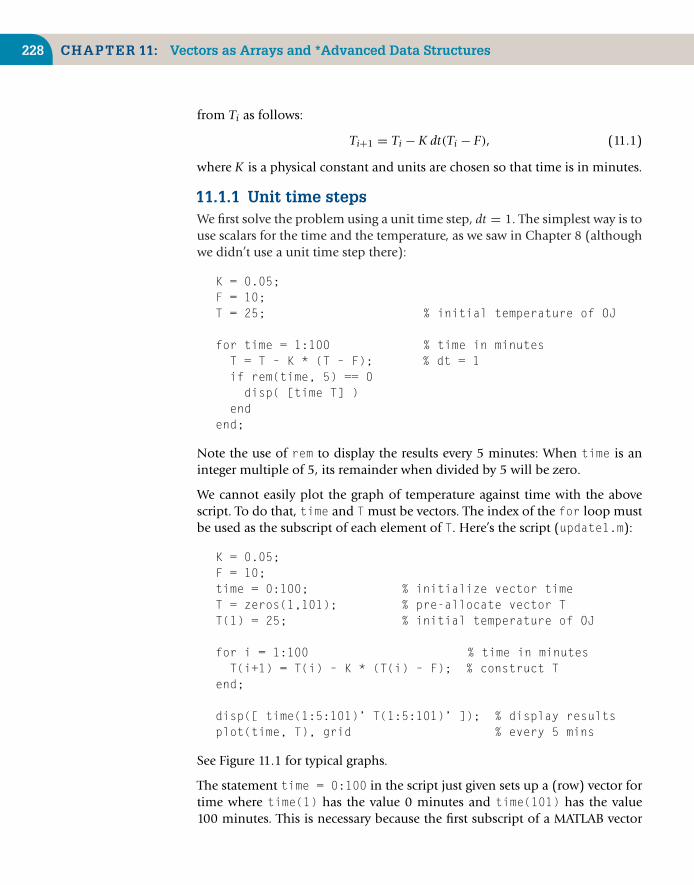
228 CHAPTER 11: Vectors as Arrays and *Advanced Data Structures
from Ti as follows:
Ti+1 = Ti − K dt(Ti − F), (11.1)
where K is a physical constant and units are chosen so that time is in minutes.
11.1.1 Unit time stepsWe first solve the problem using a unit time step, dt = 1. The simplest way is touse scalars for the time and the temperature, as we saw in Chapter 8 (althoughwe didn’t use a unit time step there):
K = 0.05;F = 10;T = 25; % initial temperature of OJ
for time = 1:100 % time in minutesT = T – K * (T – F); % dt = 1if rem(time, 5) == 0disp( [time T] )
endend;
Note the use of rem to display the results every 5 minutes: When time is aninteger multiple of 5, its remainder when divided by 5 will be zero.
We cannot easily plot the graph of temperature against time with the abovescript. To do that, time and T must be vectors. The index of the for loop mustbe used as the subscript of each element of T. Here’s the script (update1.m):
K = 0.05;F = 10;time = 0:100; % initialize vector timeT = zeros(1,101); % pre-allocate vector TT(1) = 25; % initial temperature of OJ
for i = 1:100 % time in minutesT(i+1) = T(i) – K * (T(i) – F); % construct T
end;
disp([ time(1:5:101)’ T(1:5:101)’ ]); % display resultsplot(time, T), grid % every 5 mins
See Figure 11.1 for typical graphs.
The statement time = 0:100 in the script just given sets up a (row) vector fortime where time(1) has the value 0 minutes and time(101) has the value100 minutes. This is necessary because the first subscript of a MATLAB vector

11.1 Update Processes 229
010
15
Tem
pera
ture
(de
gree
s C
)
20
25
K 5 0.030
K 5 0.150
20 40
Time (minutes)
60 80 100
FIGURE 11.1Cooling curves.
must be 1. The statement T = zeros(1,101) sets up a corresponding (row)vector for the temperature, with every element initialized to zero (again, theremust be 101 elements because the first element is for the temperature at timezero). This process, called pre-allocation, serves two important purposes:
■ It clears a vector of the same name left over from a previous run, whichcan cause a conflict when attempting to display or plot T against time ifthe vectors have different sizes. To see this, run update1 as it stands. Itshould work perfectly. Now suppose you decide to do the calculationsover a shorter time period, say 50 minutes. Remove the zerosstatement, make the following additional two changes, and rerun thescript (but don’t clear the workspace):
time = 0:50; % initialize vector time...
for i = 1:50 % time in minutes
This time you get an error message:
??? Error using ==> plotVectors must be the same lengths.
whos will reveal that time is correctly 51 by 1 but T is still 101 by 1. Theplot command naturally requires these vectors to have the same lengths.
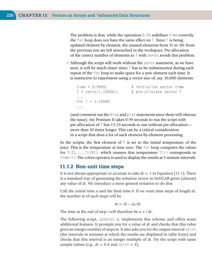
230 CHAPTER 11: Vectors as Arrays and *Advanced Data Structures
The problem is that, while the operation 0:50 redefines time correctly,the for loop does not have the same effect on T. Since T is beingupdated element by element, the unused elements from 51 to 101 fromthe previous run are left untouched in the workspace. Pre-allocationof the correct number of elements to T with zeros avoids this problem.
■ Although the script will work without the zeros statement, as we haveseen, it will be much slower since T has to be redimensioned during eachrepeat of the for loop to make space for a new element each time. Itis instructive to experiment using a vector size of, say, 10,000 elements:
time = 0:9999; % initialize vector timeT = zeros(1,10000); % pre-allocate vector T...for i = 1:10000...
(and comment out the disp and plot statements since these will obscurethe issue). My Pentium II takes 0.99 seconds to run the script withpre-allocation of T but 13.19 seconds to run without pre-allocation—more than 10 times longer. This can be a critical considerationin a script that does a lot of such element-by-element processing.
In the scripts, the first element of T is set to the initial temperature of thejuice. This is the temperature at time zero. The for loop computes the valuesfor T(2), … , T(101), which ensures that temperature T(i) corresponds totime(i). The colon operator is used to display the results at 5-minute intervals.
11.1.2 Non–unit time stepsIt is not always appropriate or accurate to take dt = 1 in Equation (11.1). Thereis a standard way of generating the solution vector in MATLAB given (almost)any value of dt. We introduce a more general notation to do this.
Call the initial time a and the final time b. If we want time steps of length dt,the number m of such steps will be
m = (b − a)/dt.
The time at the end of step i will therefore be a + i dt.
The following script, update2.m, implements this scheme and offers someadditional features. It prompts you for a value of dt and checks that this valuegives an integer number of steps m. It also asks you for the output interval opint(the intervals in minutes at which the results are displayed in table form) andchecks that this interval is an integer multiple of dt. Try the script with samesample values (e.g., dt = 0.4 and opint = 4).
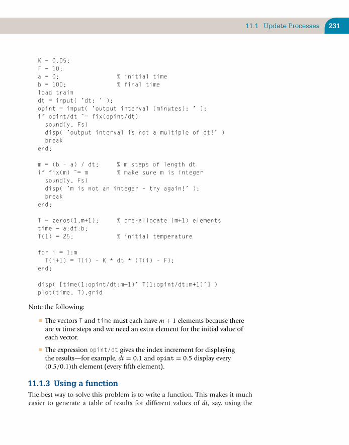
11.1 Update Processes 231
K = 0.05;F = 10;a = 0; % initial timeb = 100; % final timeload traindt = input( ’dt: ’ );opint = input( ’output interval (minutes): ’ );if opint/dt ˜= fix(opint/dt)sound(y, Fs)disp( ’output interval is not a multiple of dt!’ )break
end;
m = (b – a) / dt; % m steps of length dtif fix(m) ˜= m % make sure m is integersound(y, Fs)disp( ’m is not an integer – try again!’ );break
end;
T = zeros(1,m+1); % pre-allocate (m+1) elementstime = a:dt:b;T(1) = 25; % initial temperature
for i = 1:mT(i+1) = T(i) – K * dt * (T(i) – F);
end;
disp( [time(1:opint/dt:m+1)’ T(1:opint/dt:m+1)’] )plot(time, T),grid
Note the following:
■ The vectors T and time must each have m + 1 elements because thereare m time steps and we need an extra element for the initial value ofeach vector.
■ The expression opint/dt gives the index increment for displayingthe results—for example, dt = 0.1 and opint = 0.5 display every(0.5/0.1)th element (every fifth element).
11.1.3 Using a functionThe best way to solve this problem is to write a function. This makes it mucheasier to generate a table of results for different values of dt, say, using the
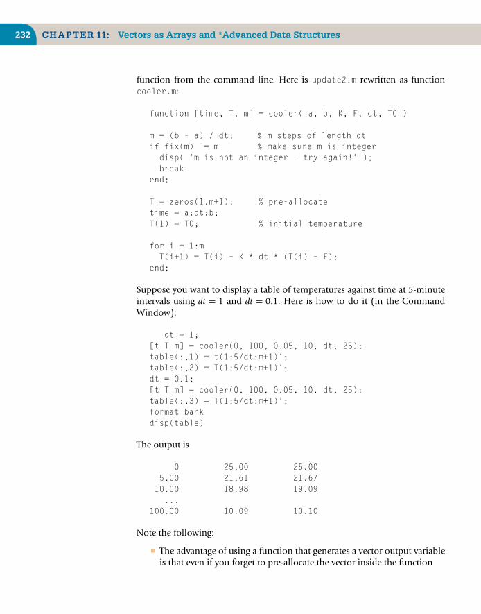
232 CHAPTER 11: Vectors as Arrays and *Advanced Data Structures
function from the command line. Here is update2.m rewritten as functioncooler.m:
function [time, T, m] = cooler( a, b, K, F, dt, T0 )
m = (b – a) / dt; % m steps of length dtif fix(m) ˜= m % make sure m is integerdisp( ’m is not an integer – try again!’ );break
end;
T = zeros(1,m+1); % pre-allocatetime = a:dt:b;T(1) = T0; % initial temperature
for i = 1:mT(i+1) = T(i) – K * dt * (T(i) – F);
end;
Suppose you want to display a table of temperatures against time at 5-minuteintervals using dt = 1 and dt = 0.1. Here is how to do it (in the CommandWindow):
dt = 1;[t T m] = cooler(0, 100, 0.05, 10, dt, 25);table(:,1) = t(1:5/dt:m+1)’;table(:,2) = T(1:5/dt:m+1)’;dt = 0.1;[t T m] = cooler(0, 100, 0.05, 10, dt, 25);table(:,3) = T(1:5/dt:m+1)’;format bankdisp(table)
The output is
0 25.00 25.005.00 21.61 21.67
10.00 18.98 19.09...
100.00 10.09 10.10
Note the following:
■ The advantage of using a function that generates a vector output variableis that even if you forget to pre-allocate the vector inside the function

11.2 Frequencies, Bar Charts, and Histograms 233
(with zeros), MATLAB automatically clears any previous versions of theoutput vector before returning from the function.
■ The variable table is a two-dimensional array (or matrix). Recall thatthe colon operator may be used to indicate all elements of a matrix in arow or column, so table(:,1) means the elements in every row andcolumn 1 (i.e., the entire first column). The vectors t and T are rowvectors, so they must be transposed before being inserted intocolumns 1 and 2. The third column is inserted in a similar way.
■ The results in the third column (for dt = 0.1) will be more accurate.
11.1.4 Exact solutionThe cooling problem has an exact mathematical solution. The temperature T(t)at time t is given by the formula
T(t) = F + (T0 − F)e−Kt (11.2)
where T0 is the initial temperature. You can insert values for this exact solutioninto a fourth column of table by vectorizing the formula as follows:
tab(:,4) = 10 + (T(1)–10)*exp(–0.05 * t(1:5/dt:m+1)’);
The enlarged table should look like this:
0 25.00 25.00 25.005.00 21.61 21.67 21.68
10.00 18.98 19.09 19.10...
Note that the numerical solution generated by Equation (11.1) gets more accu-rate as dt gets smaller. That is because Equation (11.2) (the exact solution) isderived from Equation (11.1) in the limit as dt → 0.
11.2 FREQUENCIES, BAR CHARTS, ANDHISTOGRAMS
In this section we examine graphically large arrays of data. In the next sectionwe use a bar chart. In the subsequent section we use a histogram.
11.2.1 A random walkImagine an ant walking along a straight line (the x-axis). She starts at x = 40 andmoves in steps of one unit. Each step is to the left or right with equal probability.We would like a visual representation of how much time she spends at eachposition.
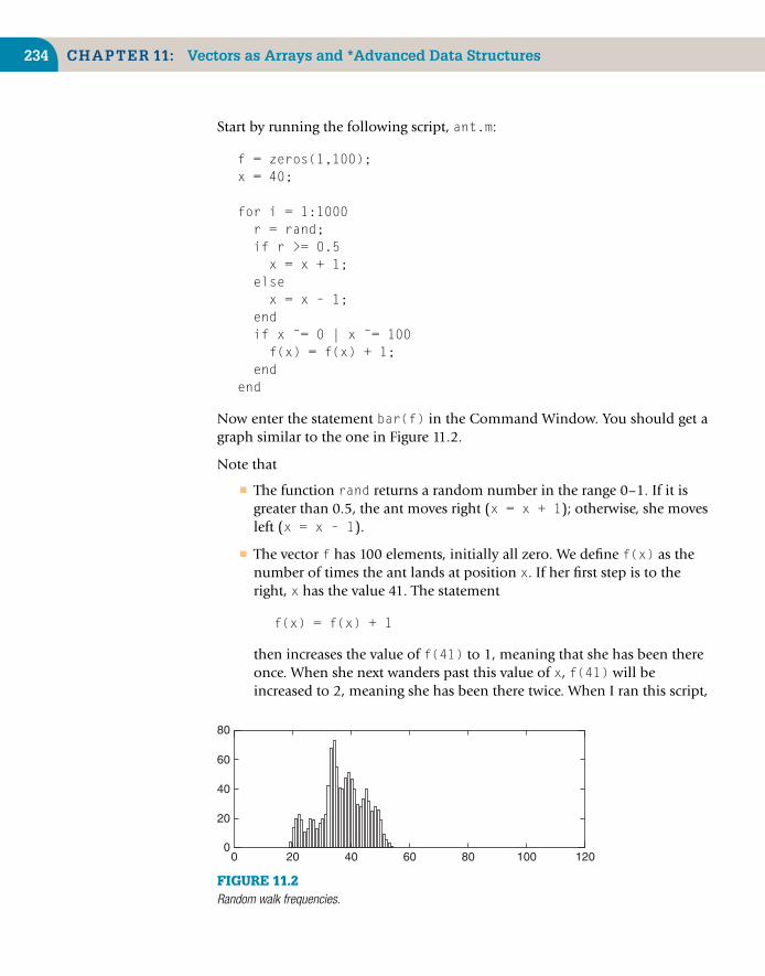
234 CHAPTER 11: Vectors as Arrays and *Advanced Data Structures
Start by running the following script, ant.m:
f = zeros(1,100);x = 40;
for i = 1:1000r = rand;if r >= 0.5x = x + 1;
elsex = x – 1;
endif x ˜= 0 | x ˜= 100f(x) = f(x) + 1;
endend
Now enter the statement bar(f) in the Command Window. You should get agraph similar to the one in Figure 11.2.
Note that
■ The function rand returns a random number in the range 0–1. If it isgreater than 0.5, the ant moves right (x = x + 1); otherwise, she movesleft (x = x – 1).
■ The vector f has 100 elements, initially all zero. We define f(x) as thenumber of times the ant lands at position x. If her first step is to theright, x has the value 41. The statement
f(x) = f(x) + 1
then increases the value of f(41) to 1, meaning that she has been thereonce. When she next wanders past this value of x, f(41) will beincreased to 2, meaning she has been there twice. When I ran this script,
00
20
40
60
80
20 40 60 80 100 120
FIGURE 11.2Random walk frequencies.

11.3 *Sorting 235
the final value of f(41) was 33—the number of times the ant wasthere.
■ f(x) is called a frequency distribution, and the graph obtained frombar(f) is called a bar graph. Each element of f is represented by avertical bar of proportional height. (See help bar.)
■ The script ant.m simulates the random movement of the ant. If yourerun it, you will get a different bar graph because rand will generate adifferent sequence of random numbers. Simulation is discussed morefully in Chapter 15.
11.2.2 HistogramsAnother helpful way of representing data is with a histogram. As an example,suppose 12 students take a test and obtain the following marks (expressed aspercentages), which are assigned to the vector m:
0 25 29 35 50 55 55 59 72 75 95 100
The statement hist(m) will draw a histogram, which shows the distribution ofmarks in 10 “bins” (categories) equally spaced between the minimum (0) andmaximum (100) in the set of data. The number of bins (10 by default) can bespecified by a second argument, such as hist(m, 25).
To generate the frequencies plotted by hist, use the following form (whichdoes not actually draw the histogram):
[n x] = hist(m)
n is a vector containing the frequences:
1 0 2 1 0 4 0 2 0 1 1
For example, there is one mark in the first bin (0–9), none in the second(10–19), and two in the third. The second output vector, x, contains the mid-points of the bins, such that bar(x, n) plots the histogram. (See Help for moredetails.)
Note the subtle difference between a histogram and a bar graph. The values plot-ted by hist are computed from the distribution of values in a vector, whereasbar generates a bar graph directly from the values themselves.
11.3 *SORTING
One standard application of an array is sorting a list of numbers, say intoascending order. Although MATLAB has its own sorting function (sort), youmay be interested in how sorting algorithms actually work.

236 CHAPTER 11: Vectors as Arrays and *Advanced Data Structures
11.3.1 Bubble SortThe basic idea is that the unsorted list is assigned to a vector. The numbers arethen ordered by a process that essentially passes through the vector many times,swapping consecutive elements that are in the wrong order until all are in theright order. Such a process is called a bubble sort because the smaller numbersrise to the top like bubbles of air in water. (In fact, in the version shown below,the largest number “sinks” to the bottom of the list after the first pass, whichreally makes it a “lead ball” sort.) There are other methods of sorting, such asthe quick sort, that may be found in most textbooks on computer science. Theseare generally more efficient than the bubble sort, but the latter’s advantage isthat it is by far the easiest to program.
A structure plan for the bubble sort is as follows:
1. Input the list X2. Set N to the length of X3. Repeat N − 1 times with counter K:
Repeat N − K times with counter J:If Xj > Xj+1 then
Swop the contents of Xj and Xj+14. Stop (the list is now sorted)
Consider a list of five numbers: 27, 13, 9, 5, and 3, initially input into thevector X. Part of MATLAB’s memory for this problem is sketched in Table 11.1,where each column shows the list during each pass. A slash in a row indicatesa change in that variable during the pass as the script works down the list. Thenumber of tests (Xj > Xj+1?) made on each pass is also shown. Work through thetable by hand with the structure plan until you understand how the algorithmworks.
Sorting algorithms are compared by calculating the number of tests (compar-isons) they carry out, since this takes up most of the sort’s execution time. Onthe K th pass of the bubble sort there are exactly N − K tests, so the total numberof tests is
Table 11.1 Memory during a Bubble Sort
1st pass 2nd pass 3rd pass 4th pass
X1 27/13 13/9 9/5 5/3X2 13/27/9 9/13/5 5/9/3 3/5X3 9/27/5 5/13/3 3/9 9X4 5/27/3 3/13 13 13X5 3/27 27 27 27Tests 4 3 2 1

11.3 *Sorting 237
1 + 2 + 3 + · · · + (N − 1) = N(N − 1)/2
(approximately N2/2 tests for large N). For five numbers there are therefore 10tests, but for 10 numbers there are 45 tests. The computer time needed goes upas the square of the length of the list.
The function M-file bubble.m below departs slightly from the structurebubble.m that will make N − 1 passes, even if the list is sorted before the lastpass. Since most real lists are partially sorted, it makes sense to check, aftereach pass, if any swaps were made. If none were, the list must be sorted sothat unnecessary (and therefore time-wasting) tests can be eliminated. In thefunction, the variable sorted is used to detect when the list is sorted, and theouter loop is coded instead as a nondeterministic while loop.
function y = bubble( x )n = length(x);sorted = 0; % flag to detect when sortedk = 0; % count the passes
while ˜sortedsorted = 1; % they could be sortedk = k + 1; % another passfor j = 1:n–k % fewer tests on each passif x(j) > x(j+1) % are they in order?temp = x(j); % no ...x(j) = x(j+1);x(j+1) = temp;sorted = 0; % a swop was made
endend
end;
y = x;
You can test it on the command line to sort, say, 20 random numbers as follows:
r = rand(1,20);r = bubble( r );
Note how bubble changes its input vector.
On my PC bubble takes 1.81 seconds to sort 200 random numbers but 7.31seconds to sort 400 numbers. This is consistent with the theoretical resultobtained above.
11.3.2 MATLAB’s sortThe built-in MATLAB function sort returns two output arguments: the sortedlist (in ascending order) and a vector containing the indexes used in the

238 CHAPTER 11: Vectors as Arrays and *Advanced Data Structures
sort—that is, the positions of the sorted numbers in the original list. If therandom numbers
r = 0.4175 0.6868 0.5890 0.9304 0.8462
are sorted with the command
[y,i] = sort(r)
the output variables are
y = 0.4175 0.5890 0.6868 0.8462 0.9304i = 1 3 2 5 4
For example, the index of the second-largest number (0.5890) is 3, which is itssubscript in the original unsorted list r. As a matter of fact, the built-in functionsmax and min also return second output variables giving indexes.
MATLAB’s sort is very fast. My PC takes 2.36 seconds to sort 1 million randomnumbers! This is because quick sort is used and the script has been compiledas a built-in function, which makes for faster code.
11.4 *STRUCTURES
Up to now we have seen arrays with only one type of element—all numeric orall character. A MATLAB structure allows you to put different kinds of data in itsvarious fields. For example, we can create a structure called student with onefield for a student’s name:
student.name = ’Thandi Mangwane’;
a second for her student ID number:
student.id = ’MNGTHA003’;
and a third for all her marks to date:
student.marks = [36 49 74];
To see the whole structure, enter its name:
student
student =name: ’Thandi Mangwane’

11.4 *Structures 239
id: ’MNGTHA003’marks: [36 49 74]
Here’s how to access her second mark:
student.marks(2)ans =
49
Note the use of the dot to separate the structure’s name from its fields whencreating it and when accessing its fields.
To add further elements to the structure, use subscripts after the structure name(the original student, Thandi Mangwane, is now accessed as student(1)):
student(2).name = ’Charles Wilson’student(2).id = ’WLSCHA007’student(2).marks = [49 98]
Note that field sizes do not have to conform across elements of a structurearray: student(1).marks has three elements, while student(2).marks hasonly two.
The student structure now has size 1 by 2: It has two elements, each a studentwith three fields. Once a structure has more than one element, MATLAB doesnot display the contents of each field when you type the structure name at thecommand line. Instead, it gives the following summary:
student
student =1x2 struct array with fields:
nameidmarks
You can also use fieldnames(student) to get this information.
A structure array can be pre-allocated with the struct function. (See Help.)
A structure field can contain any kind of data, even another structure—andwhy not? Thus, we can create a structure of courses taken by students, course,where one field is the course name, and another is a student structure withinformation on all students taking that particular course:
course.name = ’MTH101’;course.class = student;course

240 CHAPTER 11: Vectors as Arrays and *Advanced Data Structures
course =name: ’MTH101’class: [1x2 struct]
We can set up a second element of course for a different class of students:
course(2).name = ’PHY102’;course(2).class = ...
To see all the courses:
course(1:2).nameans =MTH101ans =PHY102
To see all the students in a particular course:
course(1).class(1:2).nameans =Thandi Mangwaneans =Charles Wilson
A curious function called deal “deals inputs to outputs.” You can use it togenerate comma-separated variable lists from structure fields:
[name1, name2] = deal(course(1).class(1:2).name);
(but you don’t actually need the commas here …).
The rmfield function removes fields from a structure.
11.5 *CELL ARRAYS
A cell is the most general data object in MATLAB. It may be thought of as acontainer that can hold any type of data: numeric arrays, strings, structures, orcells. An array of cells (and they almost always occur in arrays) is a cell array.You might think a cell is the same as a structure, but it is more general; also,there are notational differences (which are confusing!).
11.5.1 Assigning data to cell arraysThere are a number of ways of assigning data to cell arrays. Cell indexing isone way:
c(1,1) = {rand(3)};c(1,2) = {char(’Bongani’, ’Thandeka’)};

11.5 *Cell Arrays 241
c(2,1) = {13};c(2,2) = {student};c =
[3x3 double] [2x8 char ][13] [1x2 struct]
(assuming that the student structure created above still exists). Here the paren-theses on the left-hand side of the assignments refer in the normal way to theelements of the cell array. What is different are the curly braces on the right.They indicate the contents of a cell; on the right-hand side of an assignment theyare technically cell array constructors (remember that each element of this arrayis a cell). The first statement thus reads as “Construct a cell containing rand(3)and assign it to element 1,1 of cell array c.”
Content indexing is another way:
c{1,1} = rand(3);c{1,2} = char(’Bongani’, ’Thandeka’);c{2,1} = 13;c{2,2} = student;
Here the curly braces on the left indicate the contents of the cell element at thatparticular location. The first statement thus reads as “The contents of the cell atlocation 1,1 become rand(3).”
Curly braces can be used to construct an entire cell array in one statement:
b = {[1:5], rand(2); student, char(’Jason’, ’Amy’)}b =
[1x5 double] [2x2 double][1x2 struct] [2x5 char ]
A cell may contain another cell array; nested curly braces may be used to createnested cell arrays.
Finally, the cell function enables you to preallocate empty cell arrays:
a = cell(3,2) % empty 3-by-2 cell arraya =
[] [][] [][] []
You can then use assignment statements to fill the cells:
a(2,2) = {magic(3)}

242 CHAPTER 11: Vectors as Arrays and *Advanced Data Structures
Note that, if you already have a numeric array with a certain name, you don’twant to create a cell array of the same name by assignment without clearing thenumeric array first. If you don’t clear the numeric array, MATLAB will generatean error (it will think you are trying to mix cell and numeric syntaxes).
11.5.2 Accessing data in cell arraysYou can access cell contents using content indexing (curly braces):
r = c{1,1}r =
0.4447 0.9218 0.40570.6154 0.7382 0.93550.7919 0.1763 0.9169
To access a subset of a cell’s contents you can concatenate curly braces andparentheses if necessary:
rnum = c{1,1}(2,3)rnum =
0.9355
Here the braces (content indexing) indicate the contents of the cell array ele-ment c(1,1), which is a 3-by-3 numeric matrix. The subscripts (2,3) indicatethe appropriate element within it. Curly braces may be concatenated to accessnested cell arrays.
11.5.3 Using cell arraysCell arrays come into their own when you need to access (different types of)data as “comma-separated variable lists,” as the next example demonstrates.
The functions varargin and varargout, which allow a function to have anynumber of input or output arguments, are none other than cell arrays. Thefunctiontestvarhas a variable number of input arguments, which are doubledinto the variable number of output arguments (assuming that the number ofoutput arguments does not exceed the number of input arguments):
function [varargout] = testvar(varargin)
for i = 1:length(varargin)x(i) = varargin{i}; % unpack the input args
end
for i = 1:nargout % how many output arguments?varargout{i} = 2*x(i); % pack up the output args
end

11.5 *Cell Arrays 243
At the command line:
[a b c] = testvar(1, 2, 3, 4)a =
2b =
4c =
6
When a function is called with the input argument varargin, MATLAB auto-matically packs the list of corresponding input arguments into a cell array.Simply unpack the cell array inside the function using content indexing (curlybraces). Similarly pack up the output arguments into the cell array varargout.Note that, should your function have some compulsory input and output argu-ments, varargin and varargout must appear at the end of their respectiveargument lists.
MATLAB discusses when to use cell arrays in Organizing Data in Cell Arraysin MATLAB Help: Programming and Data Types: Structures and Cell Arrays.
11.5.4 Displaying and visualizing cell arraysThe function celldisp recursively displays the contents of a cell array. Thefunction cellplot visualizes it. Figure 11.3 depicts the contents of the cellarray c, created above. Nonempty array elements are shaded.
13
FIGURE 11.3Result of cellplot(c).

244 CHAPTER 11: Vectors as Arrays and *Advanced Data Structures
11.6 *CLASSES AND OBJECTS
MATLAB, along with most other modern programming languages, espouses thecause of object-oriented programming and has all the usual paraphernalia asso-ciated with it: classes, objects, encapsulation, inheritance, operator overloading,and so on and so forth.
Object-oriented programming is a subject that requires an entire book to doit justice. There are many excellent ones available. To see how MATLAB imple-ments object-oriented programming, consult MATLAB Help: Programmingand Data Types: MATLAB Classes and Objects.
SUMMARY
■ A MATLAB structure allows you to store different types of data in its variousfields.
■ Arrays of structures may be created.
■ A cell, the most general data object in MATLAB, can store any type of data.
■ An array of cells is called a cell array—each cell can store different types ofdata, including other cell arrays.
■ A cell array is constructed with curly braces {}.
■ The contents of a cell are accessed with content indexing (curly braces).
■ Cell elements are accessed in the usual way with parentheses (cell indexing).
■ The function cellplot visualizes a cell array.
■ MATLAB implements object-oriented programming.

CHAPTER 12
*More Graphics
The objectives of this chapter are to introduce you to
■ Handle graphics■ Editing plots■ Animation■ Saving and exporting graphs■ Color, lighting, and the camera
12.1 HANDLE GRAPHICS
The richness and power of MATLAB graphics are made possible by handle graph-ics objects. There is a very helpful section devoted to handle graphics in MATLABHelp: Graphics. What follows is of necessity a brief summary of the mainfeatures.
Handle graphics objects are the basic elements in MATLAB graphics. The objectsare arranged in a parent–child inheritance structure as shown in Figure 12.1.For example, line and text objects are children of axes objects. This is probablythe most common parent–child relationship. Axes objects define a region in afigure window and orient their children within it. The actual plots in an axesobject are line objects; the axis labels and any text annotations are text objects.It is important to be aware of this parent–child hierarchy when you manipulategraphics objects using their handles.
What is the handle of a graphics object? Whenever MATLAB creates such anobject, it automatically creates a handle to it. You can get the handle using afunction that explicitly returns it, or you can create the handle explicitly when
Copyright © 2010, Daniel T. Valentine. Published by Elsevier Ltd. All rights reserved.DOI: 10.1016/B978-0-12-374883-6.00012-6 245

246 CHAPTER 12: *More Graphics
Root
Figure
Axes
Line Surface Text
FIGURE 12.1Parent–child relationships of handle graphics objects (from top to bottom).
you draw the object. The handle itself has a floating-point representation, butits actual value need not concern you. What is more important is to save itsname and then use the handle to change or manipulate your graphics object.
The root is the only object whose handle is 0. There is only one root object,created by MATLAB at startup. All other objects are its descendants, as you cansee in Figure 12.1.
12.1.1 Getting handlesThe functions that draw graphics objects can also be used to return objecthandles:
x = 0:pi/20:2*pi;hsin = plot(x, sin(x))hold onhx = xlabel(’x’)
hsin is the handle of the line object (the sine graph), and hx is the handle ofthe text object (the x-axis label) in the current axes object. The command
figure(h)
where h is an integer, creates a new figure or makes figure h the current figure.h is the handle of the figure object.
Three functions return the handle of particular graphics objects:
■ gcf gets the handle of the current figure:
hf = gcf;

12.1 Handle Graphics 247
■ gca gets the handle of the current axes.
■ gco gets the handle of the current graphics object, which is the last onecreated or clicked on. For example, draw the sine graph above and get itshandle, hsin. Click on the graph in the figure window. Then enter thecommand
ho = gco
in the Command Window. ho should be set to the handle of the sinegraph (it should have the same numeric value as hsin).
12.1.2 Changing graphics object propertiesOnce you have the handle of a graphics object, you can use it to change theobject’s properties. As an example, draw a sine graph and get its handle, as justdemonstrated:
x = 0:pi/20:2*pi;hsin = plot(x, sin(x))
To make the lines thicker, enter the following command:
set(hsin, ’linewidth’, 4);
You should get a nice fat sine curve!
linewidth is just one of the many properties of our graphics object. To see allthe property names of an object and their current values, use get(h) where his the handle. In the case of our sine graph:
get(hsin)Color = [0 0 1]EraseMode = normalLineStyle = –LineWidth = [4]Marker = noneMarkerSize = [6]MarkerEdgeColor = autoMarkerFaceColor = noneXData = [ (1 by 41) double array]YData = [ (1 by 41) double array]ZData = []
BeingDeleted = offButtonDownFcn =Children = []Clipping = onCreateFcn =

248 CHAPTER 12: *More Graphics
DeleteFcn =BusyAction = queueHandleVisibility = onHitTest = onInterruptible = onParent = [100.001]Selected = offSelectionHighlight = onTag =Type = lineUIContextMenu = []UserData = []Visible = on
You can change any property value with the set function:
set(handle, ‘PropertyName’, PropertyValue)
The command set(handle) lists all the possible property values (where appro-priate). Also, you can get an object’s handle and change its properties all in thesame breath. For example,
set(gcf, ’visible’, ’off’)
makes the current figure invisible (without closing it—it’s still “there”). Noprizes for guessing how to make it visible again.
Property names are not case-sensitive, and you can abbreviate them to as fewletters as make them unique. For example, you can abbreviate the type propertyas ty:
get(hsin,’ty’)ans =line
(This is helpful if you don’t know what type of objects you are dealingwith.)
The different types of graphics objects don’t all have the same set of properties,although some properties are common to all, such as children, parent, andtype.
12.1.3 A vector of handlesIf a graphics object has a number of children, the get command used withthe children property returns a vector of the children’s handles. Sorting out
12.1 Handle Graphics 249
the handles is then fun and demonstrates why you need to be aware of theparent–child relationships.
As an example, plot a continuous sine graph and an exponentially decayingsine graph marked with os in the same figure:
x = 0:pi/20:4*pi;plot(x, sin(x))hold onplot(x, exp(–0.1*x).*sin(x), ’o’)hold off
Now enter the command
hkids = get(gca,’child’)
You will see that a vector of handles with two elements is returned. The questionis, which handle belongs to which plot? The answer is that the handles ofchildren of the axes are returned in the reverse order in which they are created. Thus,hkids(1) is the handle of the exponentially decaying graph while hkids(2)is the handle of the sine graph. Now let’s change the markers on the decayinggraph and make the sine graph much bolder:
set(hkids(1), ’marker’, ’*’)set(hkids(2), ’linew’, 4)
You should get the plots shown in Figure 12.2.
If you are desperate and don’t know the handles of any of your graphics objectsyou can use the findobj function to get the handle of an object with a prop-erty value that uniquely identifies it. In the original version of the plots inFigure 12.2, the decaying plot can be identified by its marker property:
hdecay = findobj(’marker’, ’o’ )
12.1.4 Graphics object creation functionsEach of the graphics objects shown in Figure 12.1 (except the root) has a cor-responding creation function, named after the object it creates. See Help fordetails.
12.1.5 ParentingBy default, all graphics objects are created in the current figure. However, youcan specify the parent of an object when you create it. For example,
axes(’Parent’, figure_handle, ... )

250 CHAPTER 12: *More Graphics
0 2 4 6 8 10 12 1421
20.8
20.6
20.4
20.2
0
0.2
0.4
0.6
0.8
1
FIGURE 12.2Result of manipulating a figure using the handles of children of axes.
creates axes with handle figure_handle. You can also move an object from oneparent to another by redefining its parent property:
set(gca, ’Parent’, figure_handle)
12.1.6 Positioning figuresAt startup, MATLAB determines the default position and size of the figure win-dow according to the size of your computer screen. You can change this bysetting the Position property of the figure object. Before you tamper withPosition, however, you need to know the dimensions of your screen—this isone of the root object’s properties:
get(0, ’screensize’)ans =
1 1 800 600
That is, the screen is 800 by 600 pixels. The units of Screensize are pixelsby default. You can (naturally) change the units by setting the root’s Unitsproperty. For example,
set(0, ’units’, ’normalized’)
normalizes the width and height of the screen to 1. This is useful when you arewriting an M-file to be run on different computer systems.

12.2 Editing Plots 251
Having sorted out the size of your screen, you can then fiddle with the figurePosition property, which is defined as a vector:
[left bottom width height]
left and bottom define the position of the first addressable pixel in the lowerleft corner of the window, specified with respect to the lower left corner ofthe screen. width and height define the size of the interior of the window(excluding the window border).
You can normalize the figure’s Unit property as well as the root’s Unit property.You can then position figures absolutely, without reference to variations inscreen size. For example, the following code normalizes units and creates twofigures in the upper half of the screen:
set(0, ’units’, ’normalized’)h1 = figure(’units’, ’normalized’, ’visible’, ’off’)h2 = figure(’units’, ’normalized’, ’visible’, ’off’)set(h1, ’position’, [0.05 0.5 0.45 0.35], ’visible’, ’on’)set(h2, ’position’, [0.53 0.5 0.45 0.35], ’visible’, ’on’)
Note that the Visible property is first set to off to avoid the figures’ beingdrawn in the default position when they are created. They are only drawn whentheir positions have been redefined. Alternatively, you can do everything whenthe figures are created:
h1 = figure(’un’, ’normalized’, ’pos’, [0.05 0.5 0.45 0.35])
12.2 EDITING PLOTS
There are a number of ways to edit plots.
12.2.1 Plot edit modeTo see how this works draw a graph—say the friendly old sine. There are severalways to activate plot edit mode:
1. Select Tools → Edit Plot in the figure window.
2. Click on the Edit Plot selection button in the figure window toolbar (thearrow pointing roughly northwest).
3. Run the plotedit command in the Command Window.
When a figure is in plot edit mode, the toolbar selection button is highlighted.Once you are in plot edit mode, select an object by clicking on it. Selectionhandles will appear on the selected object.

252 CHAPTER 12: *More Graphics
As an exercise, get the sine graph into plot edit mode and try the following:
1. Select the graph (click on it). Selection handles should appear.
2. Right-click on the selected object (the graph). A context menu appears.
3. Use the context menu to change the graph’s line style and color.
4. Use the Insert menu to insert a legend (this makes more sense whereyou have multiple plots in the figure).
5. Insert a text box inside the figure close to the graph as follows. Click onthe Insert Text selection button in the toolbar (A). The cursor changesshape to indicate that it is in text insertion mode. Move the insertionpoint until it touches the graph; then click. A text box appears. Entersome text in it.
6. Having labeled the graph, you can change the format of the labels. Selectthe label and right-click. Change the font size and style.
7. Experiment with the Insert arrow and Insert line buttons on the toolbarto see if you can insert lines and arrows in the graph.
To exit plot edit mode, click the Edit Plot button or uncheck the Edit Plot optionon the Tools menu.
12.2.2 Property EditorThe Property Editor is more general than plot edit mode. It enables you tochange object properties interactively rather than with the set function. It isideal for preparing presentation graphics.
There are numerous ways of starting the Property Editor (you may already havestumbled onto some).
■ If plot edit mode is enabled, double-click on an object or right-click onan object and select Properties from the context menu.
■ Select Figure Properties, Axes Properties, or Current Object Propertiesfrom the figure Edit menu.
■ Run the propedit command on the command line.
To experiment with the Property Editor it is useful to have multiple plots in afigure:
x = 0:pi/20:2*pi;hsin = plot(x,sin(x))hold onhcos = plot(x,cos(x))hold off
12.3 Animation 253
Once you start the Property Editor, work through the following:
1. The navigation bar at the top of the Property Editor (labeled Edit Prop-erties for:) identifies the object being edited. Click on the down arrow atthe right of the navigation bar to see all the objects in the figure. Noticethat there are two line objects. Immediately you are faced with the prob-lem of identifying them. The answer is to give them each tags by settingtheir Tag properties.
2. Go back to the figure and select the sine graph. Back in the PropertyEditor the navigation bar indicates you are editing one of the line objects.You will see three tabs below the navigation bar: Data, Style, and Info.Click the Info tab and enter a label in the Tag box (e.g., sine). PressEnter. The sine tag immediately appears next to the selected line objectin the navigation bar.
3. Give the cosine graph a tag as well (start by selecting the other lineobject).
4. Select the sine graph. This time select the Style tab and change its color,line style, line width, and markers.
5. Now select the axes object. Use the Labels tab to insert some axis labelsand the Scale tab to change the y-axis limits.
Note that if you were editing a 3D plot you would be able to use the Viewpointtab to change the viewing angle and to set various camera properties.
12.3 ANIMATION
There are three facilities for animation in MATLAB:
■ The comet and comet3 functions can be used to draw comet plots, asmentioned in Chapter 7.
■ The getframe function may be used to generate “movie frames” froma sequence of graphs. The movie function can then be used to playback the movie a specified number of times. The MATLAB onlinedocumention has the following script in MATLAB Help: Graphics:Creating Specialized Plots: Animation. It generates 16 frames from thefast Fourier transforms of complex matrices:
for k = 1:16plot(fft(eye(k+16)))axis equalM(k) = getframe;
end

254 CHAPTER 12: *More Graphics
To play it back, say five times:
movie(M, 5)
You can specify the speed of the playback among other things. See Help.
■ The most versatile (and satisfying) way of creating animations is to usethe Handle Graphics facilities.
12.3.1 Animation with Handle GraphicsTo start, run the following script, which should show the marker o tracing outa sine curve and leaving a trail behind it:
% animated sine graphx = 0;y = 0;dx = pi/40;p = plot(x, y, ’o’, ’EraseMode’, ’none’);axis([0 20*pi –2 2])for x = dx:dx:20*pi;
x = x + dx;y = sin(x);set(p, ’XData’, x, ’YData’, y)drawnow
end
Note that
■ The statement
p = plot(x, y, ’o’, ’EraseMode’, ’none’);
achieves a number of things. It plots the first point of the graph, itsaves the handle p of the plot for further reference, and it specifiesthat the Erasemode property is none (i.e., the object must not be erasedwhen it is drawn again). To achieve complete animation, set thisproperty to xor—try it now. The object is erased each time it isredrawn (in a slightly different position), creating the classic animationeffect.
■ The statement
set(p, ’XData’, x, ’YData’, y)
sets the x and y data values of the object p to the new values generatedin the for loop, and “redraws” the object. However, the object is notdrawn on the screen immediately, but joins the “event queue,” whereit waits until it is flushed out.

12.3 Animation 255
■ The drawnow function flushes the event queue and draws the object onthe screen so that we can see the fruit of our labors. As help drawnowreveals, four events flush the event queue:■ Returning to the MATLAB prompt—this is how you see all the graphs
you’ve drawn up to now■ Hitting a pause statement■ Executing a getframe command■ Executing a drawnow command
For example, you can make the marker move in a more stately fashionby replacing drawnow with pause(0.05)—0.05 seconds.
The next example comes from the Animation section of the MATLAB docu-mentation. It involves chaotic motion described by a system of three nonlineardifferential equations having a strange attractor (the Lorenz strange attractor;see Figure 12.3). The system can be written as
dydt
= Ay,
where y(t) is a vector with three components and A is a matrix dependingon y:
A(y) =
−8/3 0 y(2)
0 −10 10
−y(2) 28 −1
.
25201510
5
25210215220225
2010
0210
220
0
010
2030
4050
FIGURE 12.3Lorenz strange attractor.

256 CHAPTER 12: *More Graphics
The following script solves the system approximately using Euler’s method.Figure 12.3 shows the solution after a few thousand points have beenplotted.
A = [ –8/3 0 0; 0 –10 10; 0 28 –1 ];y = [35 –10 –7]’;h = 0.01;p = plot3(y(1), y(2), y(3), ’o’, ...
’erasemode’, ’none’, ’markersize’, 2);axis([0 50 –25 25 –25 25])hold oni = 1;while 1
A(1,3) = y(2);A(3,1) = –y(2);ydot = A*y;y = y + h*ydot;% Change colour occasionallyif rem(i,500) == 0
set(p, ’color’, [rand, rand, rand])end% Change co-ordinatesset(p, ’XData’, y(1), ’YData’, y(2), ’ZData’, y(3))drawnowi=i+1;
end
If all the points are plotted in the same color, eventually you won’t be able tosee the new points generated: A large area of the screen will be filled with thedrawing color. The color is therefore set randomly after every 500 points areplotted.
12.4 COLORMAPS
MATLAB graphics can generate a rich variety of colors. The following scriptshows a view of the Earth from space:
load earthimage(X); colormap(map)axis image
(axis image is the same as axis equal except that the plot box fits tightlyaround the data). For a variation, use hot as the argument of colormap insteadof map.

12.4 Colormaps 257
The matrix X loaded from earth is 257 by 250. Each of its elements is an integerin the range 1–64. Here is a 3-by-3 submatrix of X (somewhere in northeastAfrica):
X(39:41,100:102)ans =
14 15 1410 16 1010 10 10
The colormap function by default generates a 64-by-3 matrix with elements inthe range 0–1. The values in the three columns represent the intensities of thered, green, and blue (RGB) video components, respectively. Each row of thismatrix therefore defines a particular color by specifying its RGB components.The image function maps each element of its argument to a row in the colormapto find the color of that element. For example, X(40,101) has the value 16. Row16 of the colormap has the three values
0.6784 0.3216 0.1922
(reddish), as you can easily verify with the statements
cm = colormap(map);cm(16,:)
(The map colormap is also loaded from earth.) These RGB values specify thecolor of pixel 40 from the top and 101 from the left in the figure. Incidentally,you can use the statement
[xp yp] = ginput
to get the coordinates of a point in the figure (crosshairs appear; click on thepoint whose coordinates you want). Clicking on the point in northeast Africaresults in
xp =101.8289 % from the left (column of X)
yp =40.7032 % from the top (row of X)
Note that xp and yp correspond to the columns and rows of X, respectively.
A number of functions provided by MATLAB generate colormaps—for example,jet (the default), bone, flag, and prism. See help graph3d for a completelist. You can sample the various colormaps quite nicely with the followingstatement, which shows 64 vertical strips, each in a different color:
image(1:64),colormap(prism)

258 CHAPTER 12: *More Graphics
Or you can generate random colors:
randmap(:,1) = rand(64,1);randmap(:,2) = rand(64,1);randmap(:,3) = rand(64,1);image(1:64);colormap(randmap)
The function colorbar displays the current colormap vertically or horizontallyin the figure with your graph, indicating how the 64 colors are mapped. Try itwith earth. Note that 64 is the default length of a colormap. The functions thatgenerate colormaps have an optional parameter specifying length.
12.4.1 Surface plot colorWhen you draw a surface plot with a single matrix argument (e.g., surf(z)),the argument z specifies both the height of the surface and the color. As anexample, use the function peaks to generate a surface with a couple of peaksand valleys:
z = peaks;surf(z), colormap(jet), colorbar
The colorbar indicates that the minimum element of z (somewhat less than −6)is mapped to row 1 of the colormap (R = 0, G = 0, B = 0.5625), whereas themaximum element (about 8) is mapped to row 64 (R = 0.5625, G = 0, B = 0).
You can specify the color with a second argument the same size as the first:
z = peaks(16); % generates a 16-by-16 meshc = rand(16);surf(z, c), colormap(prism)
Here the surface is tiled with a random pattern of 16-by-16 colors from theprism colormap.
In this form of surf, each element of c is used to determine the color of thepoint in the corresponding element of z. By default MATLAB uses a processcalled scaled mapping to map from an element of z (or c) to the color in thecolormap. The details of the scaling are determined by the caxis command.For further details, see help caxis or the section Coloring Mesh and SurfacePlots in MATLAB Help: 3-D Visualization: Creating 3-D Graphs.
You can exploit the facility to specify color to emphasize surface properties. Thefollowing example is given in the MATLAB documentation:
z = peaks(40);c = del2(z);

12.5 Lighting and Camera 259
surf(z, c)colormap hot
The function del2 computes the discrete Laplacian of a surface—the Laplacianis related to the curvature of the surface. Creating a color array from the Lapla-cian means that regions with similar curvature will be drawn in the same color.Compare the surface obtained this way with that produced by the statement
surf(P), colormap(hot)
In the second case regions with similar heights about the x-y plane have thesame color.
Alternative forms of surf (and related surface functions) are
surf(x, y, z) % colour determined by zsurf(x, y, z, c) % colour determined by c
12.4.2 TruecolorThe technique of coloring by means of a colormap is called indexed coloring—a surface is colored by assigning each data point an index (row) in the colormap. Truecolor colors a surface using explicitly specified RGB triplets. Here isanother example from the MATLAB documentation (also demonstrating theuse of a multidimensional array):
z = peaks(25);c(:,:,1) = rand(25);c(:,:,2) = rand(25);c(:,:,3) = rand(25);surf(z, c)
The three “pages” of c (indicated by its third subscript) specify the respectivevalues RGB to be used to color the point in z whose subscripts are the same asthe first two subscripts in c. For example, the RGB values for the color of thepoint z(5,13) are given by c(5,13,1), c(5,13,2), and c(5,13,3).
12.5 LIGHTING AND CAMERA
MATLAB uses lighting to add realism to graphics—for example, illuminating asurface by shining light on it from a certain angle. Here are two examples fromthe MATLAB documentation:
z = peaks(25);c(:,:,1) = rand(25);c(:,:,2) = rand(25);
260 CHAPTER 12: *More Graphics
c(:,:,3) = rand(25);surf(z,c,’facecolor’,’interp’,’facelighting’,’phong’,...
’edgecolor’,’none’)camlight right
The possibilities for facelighting the surface object are none, flat (uniformcolor across each facet), gouraud, and phong. The last two are lighting algo-rithms: phong generally produces better results but takes longer to render thangouraud. Remember that you can see all of a surface object’s properties bycreating the object with a handle and using get on the handle.
This one is quite stunning:
[x y ] = meshgrid(–8 : 0.5 : 8);r = sqrt(x. ˆ2 + y. ˆ2) + eps;z = sin(r) ./ r;surf(x,y,z,’facecolor’,’interp’,’edgecolor’,’none’, ...
’facelighting’,’phong’)colormap jetdaspect([5 5 1])axis tightview(–50, 30)camlight left
For more information on lighting and camera, see Lighting as a VisualizationTool and Defining the View in MATLAB Help: 3D Visualization.
12.6 SAVING, PRINTING, AND EXPORTING GRAPHS
In this section we illustrate how to export graphics for printing and saving.
12.6.1 Saving and opening figure filesYou can save a figure generated during a MATLAB session so that you can openit in a subsequent session. Such a file has the .fig extension.
1. Select Save from the figure window File menu.
2. Make sure the Save as type is .fig.
To open the file select Open from the File menu.
12.6.2 Printing a graphYou can print everything inside a figure window frame, including axis labelsand annotations:
Summary 261
1. Select Print from the figure window File menu.
2. If you have a black and white printer, colored lines and text are “ditheredto gray,” which may not print clearly. In that case select Page Setup fromthe figure File menu. Select Lines and Text and click on Black and whitefor Convert solid colored lines to:.
12.6.3 Exporting a graphA figure may be exported in a number of graphics formats into another applica-tion, such as a text processor. You can also export it to the Windows clipboardand paste it into an application from there.
To export to the clipboard:
1. Select Copy Figure from the figure window’s Edit menu (this actioncopies to the clipboard).
2. Select Preferences from the figure’s File menu. This opens the Pref-erences panel, from which you can select Figure Copy TemplatePreferences and Copy Options Preferences to adjust the figure’s set-tings if necessary. You can also adjust settings with Page Setup from thefigure’s File menu.
To export in a specific graphics format:
1. Select Export from the figure’s File menu to invoke the Export dialoguebox.
2. Select a graphics format from the Save as type list, for example, EMF(enhanced metafiles) or JPEG. You may need to experiment to find thebest format for the target application. To insert a figure into a Worddocument, first save it in EMF or JPEG and then insert the graphicsfile into the document. This avoids the clipboard route (there are moresettings to adjust that way).
For further details consult Basic Printing and Exporting in MATLAB Help:Graphics.
SUMMARY
■ MATLAB graphics objects are arranged in a parent–child hierarchy.
■ A handle may be attached to a graphics object at creation; the handle isused to manipulate the graphics object.

262 CHAPTER 12: *More Graphics
■ If h is the handle of a graphics object, get(h) returns all current valuesof the object’s properties. set(h) shows all the possible values of theproperties.
■ The functions gcf, gca, and gco return the handles of various graphicsobjects.
■ Use set to change the properties of a graphics object.
■ A graph may be edited to a limited extent in plot edit mode, selected fromthe figure window (Tools → Edit Plot). More general editing can be donewith the Property Editor (Edit → Figure Properties from the figurewindow).
■ The most versatile way to create animations is via MATLAB’s HandleGraphics facilities. Other techniques involve comet plots and movies.
■ Indexed coloring may be done with colormaps.
■ Graphs saved to .fig files may be opened in subsequent MATLAB sessions.
■ Graphs may be exported to the Windows clipboard or to files in a varietyof graphics formats.
CHAPTER EXERCISES
12.1. Modify the line colors in the movie generated in Section 12.3. A slight modification ismade to use a handle to change the plotted object properties.
for k = 1:16hs = plot(fft(eye(k+16)));
if k <=8set(hs,’Color’,’g’)
elseset(hs,’Color’,’r’)
endaxis equalM(k) = getframe;
endmovie(M,5)
12.2. In the example provided in Section 12.3 on the Lorenz attractor, change the elementA(1, 1) = −8/3 in the A matrix to A(1, 1) = −4/3 and execute the code. Note that thischange increases the regularity of the dynamical system modeled by the Lorenz systemof equations. This illustrates how you can use MATLAB and graphics to investigateparametric changes in a system of equations that lead to interesting changes in systembehavior.

CHAPTER 13
*Graphical User Interfaces (GUIs)
The objectives of this chapter are to introduce you to the basic conceptsinvolved in writing your own graphical user interfaces, including
■ Figure files■ Application M-files■ Callback functions
The script files we have written so far have had no interaction with the userexcept for the occasional input statement. However, modern users have grownaccustomed to more sophisticated interaction with programs, through windowscontaining menus, buttons, drop-down lists, and the like. This way of interact-ing is by means of a graphical user interface, or GUI (pronounced “gooey”), asopposed to a text user interface that uses command-line based input statements.
The MATLAB online documentation has a detailed description of how to writeGUIs in MATLAB Help: Creating Graphical User Interfaces. This chapterpresents a few examples illustrating the basic concepts.
Hahn, the author of the first and second editions of this book stated that he“spent a day or two reading MATLAB’s documentation in order to write theGUIs in this chapter.” He said he seldom had such fun programming.
13.1 BASIC STRUCTURE OF A GUI
MATLAB has a facility called GUIDE (Graphical User Interface DevelopmentEnvironment) for creating and implementing GUIs. You start it from the com-mand line with the command guide. guide opens an untitled figure that
Copyright © 2010, Daniel T. Valentine. Published by Elsevier Ltd. All rights reserved.DOI: 10.1016/B978-0-12-374883-6.00013-8 263

264 CHAPTER 13: *Graphical User Interfaces (GUIs)
contains all the tools needed to create and lay out the GUI components (e.g.,push buttons, menus, radio buttons, pop-up menus, axes). These are calleduicontrols in MATLAB (for user interface controls).
GUIDE generates two files that save and launch the GUI: a FIG-file and anapplication M-file. The FIG-file contains a complete description of the GUIfigure, that is, whatever uicontrols and axes are needed for your graphicalinterface. The application M-file contains the functions required to launch andcontrol the GUI.
The GUI is controlled largely by callback functions, which are subfunctions inthe application M-file. They are written by you and determine what action istaken when you interact with a GUI component (e.g., click a button). GUIDEgenerates a callback function prototype for each GUI component you create.You then use the Editor to fill in the details.
13.2 A FIRST EXAMPLE: GETTING THE TIME
For our first example we will create a GUI with a single push button. When youclick the button, the current time should appear on it (Figure 13.1). Go throughthe following steps to place a push button in the layout area:
FIGURE 13.1Button click to show the time.

13.2 A First Example: Getting the Time 265
FIGURE 13.2GUIDE Layout Editor.
Step 1 Run guide from the command line. This action opens the LayoutEditor (Figure 13.2).
Step 2 Select the push button icon in the component palette to the left ofthe layout area. The cursor changes to a cross. Use it to select theposition of the top-left corner of the button (which has the defaultsize), or set the size of the button by clicking and dragging the cur-sor to its bottom-right corner. A button imaginatively named PushButton appears in the layout area.
Step 3 Select the push button (click on it). Right-click for its context menuand select Inspect Properties. Use the Property Inspector to changethe button’s String property to Time. The text on the button willchange to “Time.”
Note that the Tag property of the button is set to pushbutton1.This is the name GUIDE will use for the button’s callback functionwhen it generates the application M-file. If you want to use a moremeaningful name when creating a GUI that may have many suchbuttons, now is the time to change the tag.
If you change a component’s tag after generating the applicationM-file, you have to change its callback function name by hand (andall references to the callback). You also have to rename the callbackfunction in the component’s Callback property. Suppose you have

266 CHAPTER 13: *Graphical User Interfaces (GUIs)
generated an application M-file with the name myapp.m, with a pushbutton having the tag pushbutton1. The push button’s Callbackproperty will be something like
myapp(’mybutton_Callback’,gcbo,[],guidata(gcbo))
If you want to change the push button tag to Open, you will need tochange its Callback property to
myapp(’Open_Callback’,gcbo,[],guidata(gcbo))
Step 4 Back in the Layout Editor, select your button again and right-clickfor the context menu. Select Edit Callback. A dialog box appears foryou to save your FIG-file. Choose a directory and give it the filenametime.fig—make sure that the .fig extension is used.
GUIDE now generates the application M-file (time.m), which theEditor opens for you at the place where you now have to insert thecode for whatever action you want when the Time button is clicked:
function varargout = pushbutton1_Callback(h, eventdata, ...handles, varargin)
% Stub for Callback of the uicontrol handles.pushbutton1.disp(’pushbutton1 Callback not implemented yet.’)
Note that the callback’s name is pushbutton1_Callback, wherepushbutton1 is the button’s Tag property. Note also that thestatement
disp(’pushbutton1 Callback not implemented yet.’)
is automatically generated for you.
Step 5 If you are impatient to see what your GUI looks like at this stage,click Activate Figure at the right of the Layout Editor toolbar. Anuntitled window should appear with a Time button in it—click it,and the message
pushbutton1 Callback not implemented yet
should appear in the Command Window.
Step 6 Go back to the (M-file) Editor to change the pushbutton1_Callback function. Insert the following lines of code, which areexplained below:
% get timed = clock;% convert time to string

13.2 A First Example: Getting the Time 267
time = sprintf(’%02.0f:%02.0f:%02.0f’,d(4),d(5),d(6));% change the String property of pushbutton1set(gcbo,’String’,time)
The function clock returns the date and time as a six-componentvector in the format
[year month day hour minute seconds]
The sprintf statement converts the time into a string time in theusual format (e.g., 15:05:59).
Step 7 The last statement is the most important one, as it is the basis of thebutton’s action:
set(gcbo,’String’,time)
This is the button’s String property, which is displayed on it in theGUI. This is the property we want to change to the current time whenclicked.
The command gcbo (“get callback object”) returns the handle of thecurrent callback object, that is, the most recently activated uicontrol.In this case the current callback object is the button itself (it couldhave been some other GUI component). The set statement thenchanges the String property of the callback object to the stringtime just created.
Step 8 Save the application M-file and return to the Layout Editor. For com-pleteness give the entire figure a name by right-clicking anywhere inthe layout area outside the Time button. The context menu appears.Select Property Inspector. This time the Property Inspector is look-ing at the figure’s properties (instead of the push button’s properties),as indicated at the top of its window. Change the Name property tosomething suitable (like Time).
Step 9 Click Activate Figure in the Layout Editor. Your GUI should nowappear in a window entitled Time. When you click the button, thecurrent time should appear.
Step 10 If you want to run your GUI from the command line, enter theapplication M-file name.
You may have noticed that graphics objects have a Visible property. See ifyou can write a GUI with a single button that disappears when you click on it.This exercise reminds me of a project my engineering friends had when I was afirst-year student. They had to design a black box with a switch on the outside.When the switch was on, a lid opened, and a hand came out of the box toswitch it off.…

268 CHAPTER 13: *Graphical User Interfaces (GUIs)
13.3 NEWTON’S METHOD YET AGAIN
Our next example is a GUI version of Newton’s method to find a square root.When you enter the number to be square-rooted and press the Start button,some iterations appear on the GUI (Figure 13.3).
We will use the following uicontrols from the component palette in theLayout Editor:
■ A static text control to display the instruction Enter number tosquare root and press Start: (static text is not interactive, so nocallback function is generated for it).
■ An edit text control for the user to enter the number to be square-rooted.
■ A push button to start Newton’s method.
■ A static text control for the output, which will consist of several iterations.(You can of course send the output to the command line with disp.)
We will also make the GUI window resizeable. (Did you notice that you couldn’tresize the Time window in the previous example?)
Proceed as follows:
Step 1 Run guide from the command line. When the Layout Editor starts,right-click anywhere in the layout area to get the figure’s PropertyInspector, and set the figure’s Name property to Newton.
Step 2 Make the GUI resizeable by selecting Tools in the Layout Editor’s tool-bar and then Application Options. There are three Resize behavior
FIGURE 13.3Square roots with Newton’s method.

13.3 Newton’s Method Yet Again 269
options: Non-resizable (the default), Proportional, and User-specified. Select Proportional. Note that, with Proportional, whenyou resize the window the GUI components are also resized, althoughthe label size does not change.
Step 3 Place a static text, control for the instruction to the user in the layoutarea. Note that you can use the Alignment Tool in the Layout Editortoolbar to align controls accurately. You can also use the Snap to Gridoption in the Layout menu. If Snap to Grid is checked, any objectmoved to within 9 pixels of a grid line jumps to it. You can changethe grid spacing with Layout → Grid and Rulers → Grid size.
Use the Property Inspector to change the static text control’s Stringproperty to Enter number to square root and press Start.
Step 4 Place an edit text control in the layout area for the user to inputthe number to be square-rooted. Set its String property to blank.Note that you don’t need to activate the Property Inspector for eachcontrol. Once the Property Inspector has been started it switches towhichever object you select in the layout area. The tag of this com-ponent will be edit1 since no other edit text components have beencreated.
Step 5 Activate the figure at this stage (use the Activate Figure button in theLayout Editor toolbar), and save it under the name Newton.fig.The application M-file should open in the Editor. Go to theedit1_Callback subfunction and remove the statement
disp(’edit1 Callback not implemented yet.’)
No further coding is required in this subfunction since action is to beinitiated by the Start button. Remember to remove the disp statementfrom each callback subfunction as you work through the code.
Step 6 Insert another static text control in the layout area for the output ofNewton’s method. Make it long enough for five or six iterations. Setits String property to Output and its HorizontalAlignment toleft (so that output will be left-justified). Note its tag, which shouldbe text2 (text1 being the tag of the other static text control).
Step 7 Place a push button in the layout area. Set its String property toStart. Its tag should be pushbutton1.
Step 8 Activate the figure again so that the application M-file is updated. Wenow have to program the pushbutton1_Callback subfunction to■ Get the number to be square-rooted from the edit text control■ Run Newton’s method to estimate the square root of this number

270 CHAPTER 13: *Graphical User Interfaces (GUIs)
■ Put the output of several iterations of Newton’s method in theOutput static text control
■ Clear the edit text control in readiness for the next number to beentered by the user
These actions are achieved by the following code:
function varargout = pushbutton1_Callback(h, eventdata, ...handles, varargin)
% Stub for Callback of the uicontrol handles.pushbutton1.
a = str2num(get(handles.edit1,’String’));x = a; % initial guess
for i = 1:8x = (x + a/x)/2;str(i) = {sprintf(’%g’,x)};
end
set(handles.edit1,’String’,’’);set(handles.text2,’String’,str);
Regarding the last step, if you read the helpful comments generated in theapplication M-file, you know that the input argument handles is a structurecontaining handles of GUI components, using their tags as fieldnames. Thismechanism enables the various components to communicate with each otherin the callback subfunctions, which is why it is not a good idea to changea tag after its callback subfunction has been generated. If you do, you thenneed to change the name of the callback function as well as any references toits handle.
When you type anything into an edit text control, its String property isautomatically set to whatever you type. The first statement:
a = str2num(get(handles.edit1,’String’));
uses the handle of the edit text control to get its String property (assuming itto have been correctly entered—we are not trying to catch any user errors here).The str2num function converts this string to the number a. A for loop thengoes through eight iterations of Newton’s method to estimate a’s square root.
The variable x in the loop contains the current estimate. sprintf converts thevalue of x to a string using the g (general) format code. The resulting string isstored in the ith element of a cell array str. Note the use of curly braces toconstruct the cell array. This is the easiest way to put multiple lines of text intoan array for sending to the text2 static text.

13.4 Axes on a GUI 271
The statement
set(handles.edit1,’String’,’’);
clears the display in the edit text control. The statement
set(handles.text2,’String’,str);
sets the String property of the text2 static text control to the cell arraycontaining the output.
Once you have completed your Newton’s GUI, save it and reactivate it to test it.
13.4 AXES ON A GUI
This example demonstrates how to plot graphs in axes on a GUI. We want onebutton to draw the graph, one to toggle the grid on and off, and one to clearthe axes (Figure 13.4). The only new feature in this example is how to plot inaxes that are part of the GUI. We address this issue first.
FIGURE 13.4Axes on a GUI.

272 CHAPTER 13: *Graphical User Interfaces (GUIs)
Step 1 Open a new figure in the GUIDE Layout Editor. Right-click anywherein the layout area to open the figure’s Property Inspector. Note thatthe figure has a HandleVisibility property set to off by default.This prevents any drawing in the figure. For example, you probablydo not want plot statements issued at the command line to be drawnon the GUI. However, you can’t at the moment draw on the GUI fromwithin it either. The answer is to set the figure’s HandleVisibilityproperty to callback. This allows any GUI component to plot graphson axes that are part of the GUI while still protecting the GUI frombeing drawn on from the command line.
Step 2 Place an axes component on the GUI. Its HandleVisibility shouldbe on.
Step 3 Place a push button (tag pushbutton1) on the GUI and change itsString property to Plot. Save the figure (if you have not already)under the name Plotter and generate the application M-file. Edit thepush button’s callback subfunction to draw any graph (e.g., sin(x)).
Step 4 Place pushbutton2 on the GUI to toggle the grid, and put thecommand grid in its callback subfunction.
Step 5 Put pushbutton3 on the GUI with the command cla to clear theaxes.
Step 6 Save and reactivate the figure. Test it. Set the figure’s Handle-Visibility to off, activate the figure, and see what happens. Notethat the figure object’s IntegerHandle property is set to off. Thismeans that even if HandleVisibility is on, you can’t plot on theaxes from the command line (or another GUI) because a figure needsan integer handle to be accessed. If you want to be able to draw onyour GUI from the command line, just set the figure’s IntegerHandleto on.
13.5 ADDING COLOR TO A BUTTON
The final example in this chapter shows you how to add an image to a button.
1. Create a GUI with a single push button.
2. Set the button’s Units property to pixels.
3. Expand the button’s Position property and set width to 100 andheight to 50.
4. Insert the following code in the button’s callback subfunction:
a(:,:,1) = rand*ones(50,100);a(:,:,2) = rand*ones(50,100);

Summary 273
a(:,:,3) = rand*ones(50,100);set(h,’CData’,a);
5. The matrix a defines a Truecolor image the same size as the push but-ton, with each pixel in the image the same (random) color. The thirddimension of a sets the RGB video intensities. If, for example, you preferthe button to be a random shade of green, try
a(:,:,1) = zeros(50,100);a(:,:,2) = rand*ones(50,100);a(:,:,3) = zeros(50,100);
6. The input argument h of the callback subfunction is the callback object’shandle (obtained from gcbo).
7. Add an image to a toggle button control if you like.
SUMMARY
■ GUIs are designed and implemented by MATLAB’s GUIDE facility.
■ The guide command starts the Layout Editor, which is used to design GUIs.
■ GUIDE generates a FIG-file, which contains the GUI design, and anapplication M-file, which contains the code necessary to launch and controlthe GUI.
■ You launch the GUI by running its application M-file.
■ Many GUI components have callback subfunctions in the applicationM-file, where you write the code to specify the components’ actions.
■ You use the Property Inspector to set a GUI component’s properties at thedesign stage.
■ The handles of all GUI components are fields in the handles structure inthe application M-file. They are available to all callback subfunctions andenable you to find and change components’ properties.

2PART
Applications
Since this is an introductory course, the applications discussed in this partare not extensive; they are illustrative. You should recognize that the kinds ofproblems you can actually solve with MATLAB are much more challengingthan the examples provided. More is said on this matter at the beginning ofChapter 14. The goal of this part is to scratch the surface of the true power ofMATLAB and to show how you can use it in a variety of ways.

CHAPTER 14
Dynamical Systems
The objective of this chapter is to discuss the importance of learning toolslike MATLAB.
In this chapter we examine MATLAB’s application to four relatively simpleproblems in engineering: the deflection of a cantilever beam subject to a uni-form load; a single-loop closed electrical circuit; the free-fall problem; and anextension of the projectile problem discussed in Chapter 3. The first probleminvolves a structural element you investigate in a first course in engineeringmechanics—the cantilever beam, which is one of the primary elements of engi-neered structures such as buildings and bridges. We examine the deflection ofthis beam with a constant cross-section when subject to a uniform distributionof load (e.g., its own weight).
The second problem involves the equation that describes the “flow” of electricalcurrent in a simple closed-loop electrical circuit. You meet this type of problemin a first course in electrical science.
The third problem involves the free fall of an object in a gravitational field withconstant acceleration, g. This is one of the first problems you encounter in afirst course in physics. We examine the effect of friction on the free-fall problemand learn that with friction (i.e., air resistance) the object can reach a terminalvelocity.
The fourth problem extends the projectile problem that takes into account airresistance (you learn about air resistance in your first course in fluid mechanics).You will learn why golfers don’t hit the ball from the tee at 45 degrees from thehorizontal (which is the optimum angle for the furthest distance of travel of aprojectile launched in frictionless air).Copyright © 2010, Daniel T. Valentine. Published by Elsevier Ltd. All rights reserved.DOI: 10.1016/B978-0-12-374883-6.00014-X 277

278 CHAPTER 14: Dynamical Systems
14.1 CANTILEVER BEAM
In this section we want to examine the problem of the cantilever beam. Thebeam and its deflection under load are illustrated in Figure 14.1, which is gener-ated by the script M-file created to solve the problem posed next. Many structuralmechanics formulae are available in Formulas for Stress and Strain, fifth edition,by Raymond J. Roark and Warren C. Young (McGraw-Hill 1982).
For a uniformly loaded span of a cantilever beam attached to a wall at x = 0with the free end at x = L, the formula for the vertical displacement from y = 0under the loaded condition, with y the coordinate in the direction oppositethat of the load, can be written as follows:
Y = y 24EIwL4 = −(
X4 − 4 X3 + 6 X2),
where X = x/L, E is a material property known as the modulus of elasticity; Iis a geometric property of the cross-section of the beam known as the momentof inertia; L is the length of the beam extending from the wall on which itis mounted; and w is the load per unit width of the beam (this is a two-dimensional analysis). The formula was put into dimensionless form to answerthe following question: What is the shape of the deflection curve when the beamis in its loaded condition, and how does it compare with its unloaded perfectlyhorizontal orientation? The answer will be provided graphically.
0 0.5 1 1.524
23.5
23
22.5
22
21.5
21
20.5
0
0.5
1Deflection of a cantilever beam
X
Y
Unloaded cantilever beamUniformly loaded beam
FIGURE 14.1Vertical deflection of a uniformly loaded cantilever beam.

14.2 Electric Current 279
The problem is easily solved using the following script (the results are plottedin Figure 14.1):
%% The deflection of a cantilever beam under a uniform load% Script by D.T.V. ........ September 2006%% Step 1: Select the distribution of X’s from 0 to 1% where the deflections to be plotted are to be determined.%X = 0:.01:1;%% Step 2: Compute the deflections Y at each X. Note that YE% is the unloaded position of all points on the beam.%Y = – ( X.ˆ4 – 4 * X.ˆ3 + 6 * X.ˆ2 );YE = 0;%% Step 3: Plot the results to illustrate the shape of the% deflected beam.%plot([0 1],[0 0],’––’,X,Y,’LineWidth’,2)axis([0,1.5,–4, 1]),title(’Deflection of a cantilever beam’)xlabel(’X’),ylabel(’Y’)legend(’Unloaded cantilever beam’,’Uniformly loaded beam’)%% Step 4: Stop
It looks like the beam is deflected tremendously, but the actual deflection is notso dramatic once the actual material properties are substituted to determine yand x in, say, meters. The scaling (i.e., rewriting the equation in dimensionlessform in terms of the unitless quantities Y and X) provides insight into the shapeof the curve. In addition, the shape is independent of the material as long as thematerial has uniform properties and the geometry has a uniform cross-sectionalarea (e.g., a rectangular area of height h and width b that is independent of thedistance along the span (or length) L).
14.2 ELECTRIC CURRENT
In electrical science you investigate circuits with a variety of components. Inthis section we will solve the governing equation to examine the dynamics of asingle, closed-loop electrical circuit. The loop contains a voltage source, V (e.g.,a battery), a resistor, R (i.e., an energy dissipation device), an inductor, L (i.e., anenergy storage device), and a switch that is instantaneously closed at time t = 0.

280 CHAPTER 14: Dynamical Systems
From Kirchoff ’s law, as described in Circuits, Devices, and Systems by Ralph J.Smith (John Wiley & Sons, 1967), the equation describing the response of thissystem from an initial state of zero current is
Ldidt
+ Ri = V
where i is the current. At t = 0 the switch is engaged to close the circuit andinitiate the current. At this instant of time the voltage is applied to the resistorand inductor (which are connected in series) instantaneously. The equationdescribes the value of i as a function of time after the switch is engaged. For thepresent purpose, then, we want to solve it to determine i versus t graphically.Rearranging the equation, we get
didt
+ RL
i = VL
The solution, by inspection (another method that you learn when you studydifferential equations), is
i = VR
(1 − e− R
L t)
which is checked with the following script:
%% Script to check the solution to the soverning% equation for a simple circuit, i.e., to check% that% i = (V/R) * (1 – exp(–R*t/L))%% is the solution to the following ODE%% di/dt + (R/L) * i – V/L = 0%% Step 1: We will use the Symbolics tools; hence,% define the symbols as follows%
syms i V R L t%% Step 2: Construct the solution for i%
i = (V/R) * ( 1 – exp(–R*t/L) );%% Step 3: Find the derivative of i%
didt = diff(i,t);%

14.3 Free Fall 281
% Step 4: Sum the terms in ODE%
didt + (R/L) * i – V/L;%% Step 5: Is the answer ZERO?%
simple(ans)%% Step 6: What is i at t = 0?%subs(i,t,0)%% REMARK: Both answers are zero; hence,% the solution is correct and the% initial condition is correct.%% Step 7: To illustrate the behavior of the% current, plot i vs. t for V/R = 1% and R/L = 1. The curve illustrates% the fact that the current approaches% i = V/R exponentially.%
V = 1; R = 1; L = 1;t = 0 : 0.01 : 6;i = (V/R) * ( 1 – exp(–R.*t/L) );plot(t,i,’ro’), title(Circuit problem example)
xlabel(’time, t’),ylabel(’current, i’)%
Running this script will prove that the solution is correct. Figure 14.2 illustratesthe solution.
14.3 FREE FALL
In this section we will use MATLAB to investigate the problem of free fall withfriction (or air resistance) and to check the theoretical results found in theliterature. We want to determine the effect of air resistance on the distanceof free fall in 5 seconds from a location y = 0, where the object is initiallyat rest (y is in the direction of gravity). Hence, we want to determine thedistance, y = L that an object falls from a state of rest with and without airresistance.
In Introduction to Theoretical Mechanics by R. A. Becker (McGraw-Hill 1954), theequations for free fall are given. The three cases of interest are as follows:

282 CHAPTER 14: Dynamical Systems
0 1 2 3 4 5 60
0.1
0.2
0.3
0.4
0.5
0.6
0.7
0.8
0.9
1Circuit problem
Time, t
Cur
rent
,i
FIGURE 14.2Exponential approach to steady current condition of a simple RL circuit with an instantaneously appliedconstant voltage.
Case 1. Without air resistance:
a = d2ydt2 = g, v = dy
dt= gt, y = 1
2gt2
where a is the acceleration of the object, v is its speed, and y is thedistance of its free fall from the start of motion at t = 0.
Case 2. With resistance proportional to the linear power of velocity:
a = d2ydt2 = g − k
dydt
, v = dydt
= gk
(1 − e−kt
), y = g
kt − g
k2
(1 − e−kt
)
Case 3. With resistance proportional to the second power of velocity:
a = d2ydt2 = g − k
(dydt
)2
, v = dydt
= 12
gk
tanh(
gk2
t)
, y = 1k
loge[cosh
(gkt/2
)]
For all three cases, the initial condition is y = v = 0 at t = 0. (You will learn moreabout ordinary differential equations in your third semester of mathematics. Inaddition, in a first course in fluid mechanics you will learn some of the details

14.3 Free Fall 283
about air resistance. In particular, for air resistance associated with “laminarflow” problems, case 2 applies. In many practical situations, case 3 is usuallythe one of interest; this is where “turbulent flow” is important.)
Let us consider the following problem: Assume the above equations arecorrect. Note that they are written for a unit of mass. Also assume g = 9.81m/s2 and k = 0.2 for the air-drag parameter. Finally, answer the following:
■ What is y in meters for t = 5 seconds of free fall for the three cases?
■ What are the terminal speeds in meters per second for cases 2 and 3 forthe specified air-drag parameter?
■ Is the terminal speed reached at t = 5 seconds?
Note that
■ The terminal speeds are g/k and (g/k)/2 for cases 2 and 3, respectively,where the terminal speed is the time-independent, or steady, speedreached after a sufficient distance of free fall. This is the speed at whichthe gravitational force balances the air resistance force. From Part 1, theEssentials, we learned that MATLAB is quite useful in this type ofproblem because it has the capability of computing the elementaryfunctions in the above formulae.
■ As part of providing an answer to the questions raised, we want toexamine the distance of free fall within the 5 seconds of flight timeusing the equations for y given above. If we examine the influence of airresistance on free fall graphically, we need to plot the distance y versus tfrom t = 0 to t = 5 seconds. We plot all three curves on one figure fordirect comparison, and show that for a short period of time(significantly less than 5 seconds) after the onset of motion, all threecurves are on top of each other. We also show that at t = 5 seconds thedistances of free fall are quite different.
The steps in the structure plan and the MATLAB code are as follows:
%% Free fall analysis (saved as FFall.m):% Comparison of exact solutions of free% fall with zero, linear and quadratic% friction for t = 0 to 5 seconds.%% Script by D. T. V. ......... September 2006.% Revised by D.T.V. .......... November 2008.%% Step 1: Specify constants%

284 CHAPTER 14: Dynamical Systems
% Friction coefficient provided in the problem statement.k = 0.2;% Acceleration of gravity in m/s/s.g = 9.81;%% Step 2: Selection of time steps for computing solutions%dt = .01;%% Step 3: Set initial condition (the same for all cases)%t(1) = 0.; v(1) = 0.; y(1) = 0.;%t = 0:dt:5;%% Step 4: Compute exact solutions at each time step% from t = 0 to 5.%% (a) Without friction:%
v = g * t;y = g * t.ˆ2 * 0.5;
%% (b) Linear friction%
velf = (g/k) * (1. – exp(–k*t));yelf = (g/k) * t – (g/(kˆ2)) * (1.–exp(-k*t));
%% (c) Quadratic friction%
veqf = sqrt(g/k) * tanh( sqrt(g*k) * t);yeqf = (1/k) * log(cosh( sqrt(g*k) * t) );
%% Step 5: Computation of the terminal speeds% (cases with friction)%
velfT = g/k;veqfT = sqrt(g/k);
%% Step 6: Graphical comparison%plot(t,y,t,yelf,t,yeqf)title(’Fig 1. Comparison of results’)xlabel(’ Time, t’)ylabel(’ Distance, y ’)
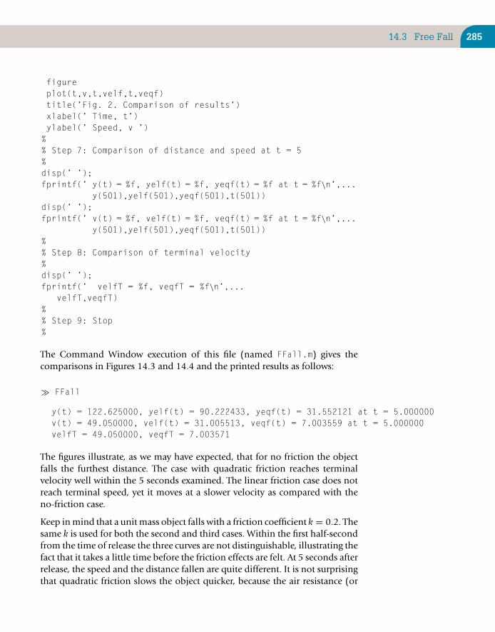
14.3 Free Fall 285
figureplot(t,v,t,velf,t,veqf)title(’Fig. 2. Comparison of results’)xlabel(’ Time, t’)ylabel(’ Speed, v ’)
%% Step 7: Comparison of distance and speed at t = 5%disp(’ ’);fprintf(’ y(t) = %f, yelf(t) = %f, yeqf(t) = %f at t = %f\n’,...
y(501),yelf(501),yeqf(501),t(501))disp(’ ’);fprintf(’ v(t) = %f, velf(t) = %f, veqf(t) = %f at t = %f\n’,...
y(501),yelf(501),yeqf(501),t(501))%% Step 8: Comparison of terminal velocity%disp(’ ’);fprintf(’ velfT = %f, veqfT = %f\n’,...
velfT,veqfT)%% Step 9: Stop%
The Command Window execution of this file (named FFall.m) gives thecomparisons in Figures 14.3 and 14.4 and the printed results as follows:
� FFall
y(t) = 122.625000, yelf(t) = 90.222433, yeqf(t) = 31.552121 at t = 5.000000v(t) = 49.050000, velf(t) = 31.005513, veqf(t) = 7.003559 at t = 5.000000velfT = 49.050000, veqfT = 7.003571
The figures illustrate, as we may have expected, that for no friction the objectfalls the furthest distance. The case with quadratic friction reaches terminalvelocity well within the 5 seconds examined. The linear friction case does notreach terminal speed, yet it moves at a slower velocity as compared with theno-friction case.
Keep in mind that a unit mass object falls with a friction coefficient k = 0.2. Thesame k is used for both the second and third cases. Within the first half-secondfrom the time of release the three curves are not distinguishable, illustrating thefact that it takes a little time before the friction effects are felt. At 5 seconds afterrelease, the speed and the distance fallen are quite different. It is not surprisingthat quadratic friction slows the object quicker, because the air resistance (or

286 CHAPTER 14: Dynamical Systems
0 1 2 3 4 50
20
40
60
80
100
120
140Comparison of y results
Time, t
Dis
tanc
e, y
FIGURE 14.3Comparison of free-fall distance: top curve, no friction; middle curve, linear friction; bottom curve,quadratic friction.
0 1 2 3 4 50
5
10
15
20
25
30
35
40
45
50Comparison of v results
Time, t
Spe
ed,v
FIGURE 14.4Comparison of free-fall speed: top curve, no friction; middle curve, linear friction; bottom curve, quadraticfriction.
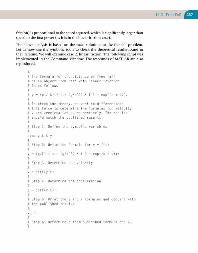
14.3 Free Fall 287
friction) is proportional to the speed squared, which is significantly larger thanspeed to the first power (as it is in the linear-friction case).
The above analysis is based on the exact solutions to the free-fall problem.Let us now use the symbolic tools to check the theoretical results found inthe literature. We will examine case 2, linear friction. The following script wasimplemented in the Command Window. The responses of MATLAB are alsoreproduced.
%% The formula for the distance of free fall% of an object from rest with linear friction% is as follows:%% y = (g / k) * t – (g/kˆ2) * [ 1 – expˆ(– k t)].%% To check the theory, we want to differentiate% this twice to determine the formulas for velocity% v and acceleration a, respectively. The results% should match the published results.%% Step 1: Define the symbolic variables%syms g k t y%% Step 2: Write the formula for y = f(t)%y = (g/k) * t – (g/kˆ2) * ( 1 – exp(–k * t));%% Step 3: Determine the velocity%v = diff(y,t);%% Step 4: Determine the acceleration%a = diff(v,t);%% Step 5: Print the v and a formulas and compare with% the published results%v, a%% Step 6: Determine a from published formula and v.%
288 CHAPTER 14: Dynamical Systems
a2 = g – k * v;% Step 7: Simplify to simplest forma2 = simple(a2)%% Step 6: Stop. REMARK: Results compare exactly. The% results printed in the command window after executing% this script are as follows:% v = g/k–g/k*exp(–k*t)% a = g*exp(–k*t)% a2 = g/exp(k*t)% These results verify the conclusion that the published% formulas are correct.%
We next consider an approximate method for solving the linear-friction case.This procedure is something you could implement if you didn’t have the exactsolution. More on numerical methods is provided in Chapter 17.
The equations for free-fall acceleration and velocity are differentials. The fol-lowing approximate analysis of a differential equation is called finite-difference.Let’s consider free fall with linear friction (i.e., air drag that is linearly pro-portional to the speed of free fall). The formula (or equation) for this andits exact solution were given above. In the following analysis a script to solvethis problem by the approximate method is written and executed for the sameinterval of time. The approximate solution is compared with the exact solutiongraphically.
For a unit mass, the formula that describes the velocity of free fall from restwith air resistance proportional to the linear power of velocity can be writtenas follows:
dvdt
= g − kv,
We approximate this equation by inverting the fundamental theorem of differ-ential calculus. That is, we rewrite it in terms of the definition of a derivativebefore the appropriate limit is taken. What is meant is that we write this equationfor a small interval of time �t = t(n + 1) − t(n) as follows:
dvdt
≈ v(n + 1) − v(n)
�t= g − k
(v(n + 1) + v(n)
2
)
where the value identified by the integer n is the value of v at the beginningof the time interval (i.e., v(n) at t(n)). The value identified by n + 1 is thevalue of v at the end of the time interval (i.e., v(n + 1) at t(n + 1)). This isan initial-value problem, so the value of v is known at t(n). Knowing v(n) at

14.3 Free Fall 289
t(n), and specifying t(n + 1), the value v(n + 1) can be calculated by solving thefinite-difference equation for v(n + 1) given above. The solution will dependon the size of �t. This formula gives us v(n + 1).
We next need to solve for y(n + 1) from the definition of v (an approximateform of dy/dt). The average value of v over the interval of time, �t, can bewritten in terms of y as follows:
dydt
≈ y(n + 1) − y(n)
�t= v(n + 1) + v(n)
2
Rearranging this equation, we get a formula for y(n + 1) in terms of v(n + 1),v(n), y(n), and �t. Given the initial condition—that is, y(n) and v(n) at t(n)—wecompute v(n + 1) with the first difference equation followed by y(n + 1) withthe last equation. Note that the new values become the initial condition for the nexttime step. This procedure is repeated until the overall time duration of interest isreached (in this case t = 5). The script file to implement this procedure is givennext. The M-file is executed and the results are plotted on the same graph withthe exact solution. As shown, the comparison is remarkable. This is not alwaysthe case when approximate methods are used. The comparison is, of course,encouraging because we usually do not have exact results and need to resort tonumerical approximations in our work.
The script file applied to examine the difference between the approximatemethod and the exact result is as follows:
%% Approximate and exact solution comparison of% free fall with linear friction for t = 0 to 5.%% Script by D. T. V. .......... September 2006.% Revised by D.T.V. ............ November 2008.%% Step 1: Specified constants%k = 0.2;g = 9.81;%% Step 2: Selection of time step for approximate solution% dt = t(n+1) – t(n)dt = 0.01;%% Step 3: Initial condition%

290 CHAPTER 14: Dynamical Systems
t(1) = 0.;v(1) = 0.;y(1) = 0.;%% Step 3: Sequential implementation of the approximate% solution method by repeating the procedure 500 times% (using a for loop).%for n = 1:1:500
t(n+1) = t(n) + dt;v(n+1) = (v(n) + dt * (g–0.5*k*v(n)) )/(1.+dt*0.5*k);y(n+1) = y(n) + dt * 0.5 * (v(n+1) + v(n));
end%% Step 4: Exact solution over the same interval of time:%
ye = (g/k) * t – (g/(kˆ2)) * (1.–exp(–k*t));%% Step 5: Graphical comparison:%plot(t,y,’o’,t,ye)title(’Comparison of numerics w/ exact results’)xlabel(’ Time, t’)ylabel(’ Distance of free fall from rest, y’)%% Step 6: Comparison of distance at t=5%disp(’ ’);fprintf(’ y(t) = %f, ye(t) = %f at t = %f \n’,...
y(501),ye(501),t(501))%% Step 7: End of script by DTV.%
The plot command in this script produced Figure 14.5. The exact solution is agreen line through the center of the circle.
In summary, examination of the free-fall problem illustrates the application andthe checking of formulae reported in the literature. An approximate methodsolves the same problem, illustrating a method that would be necessary if exactformulas were not found. Finally, the approximate method can certainly beimproved by utilizing the ordinary differential equation solvers available inMATLAB. Examples of this type of procedure are given in Chapter 17. Otherexamples are in MATLAB; Help found via the question mark in the toolbar onthe desktop (as already mentioned).

14.4 Projectile with Friction 291
0 1 2 3 4 50
10
20
30
40
50
60
70
80
90
100Comparison of numerics with exact results
Time, t
Dis
tanc
e of
free
fall
from
res
t, y
FIGURE 14.5Comparison of free-fall distance: line, exact distance; circles, finite-difference approximate solution.
14.4 PROJECTILE WITH FRICTION
Let’s examine the projectile problem again—in this case the effect of air resis-tance on the flight of a projectile such as a golf ball. For a unit mass, the formulaethat describe the trajectory of a projectile in a gravitational field, g, with airresistance in the opposite direction of motion (proportional to the speed of theprojectile in the direction of motion squared) are as follows:
u = dx/dt,
v = dy/dt,
du/dt = −ku ∗√
u2 + v2,
dv/dt = −kv ∗√
u2 + v2 − g.
The location of the projectile (the golf ball) is initially at x = 0, y = 0. It islaunched at a speed Vs in the direction of angle θ as measured from the hori-zontal. The coordinate x is in the horizontal direction parallel to the ground.The coordinate y is in the direction perpendicular to x pointing toward the sky.Hence, the gravitational acceleration is in the negative y direction. For a givenlaunch speed and direction, we wish to estimate the range (or distance) the balltravels in the x direction when it first hits the ground. To do this we approximate

292 CHAPTER 14: Dynamical Systems
the four equations similarly to how we treated the free-fall problem in the lastsection.
The solution method is given in detail in the script following (golf.m):
%% "The Golf ball problem"% Numerical computation of the trajectory of a% projectile launched at an angle theta with% a specified launch speed. They are:% theta = launch angle in degrees.% Vs = launch speed.%% Script by D. T. V. ...... September 2006.% Revised by D.T.V. ...... November 2008.%% Equations of motion:% u = dx/dt. v = dy/dt. g is in the opposite% direction of y. x = y = 0 is the location of% the tee. k is the coefficient of air drag. It% is assumed to be constant. Friction is assumed% to be proportional to the speed of the ball% squared and it acts in the opposite direction% of the direction of motion of the ball. The% components of acceleration are thus:% du/dt = – [k (uˆ2 + vˆ2) * u/sqrt(uˆ2+vˆ2)].% dv/dt = – [k (uˆ2 + vˆ2) * v/sqrt(uˆ2+vˆ2)] – g.%% INPUT DATA% Specified constants:k = 0.02;g = 9.81;dt = 0.01;%% Input the initial condition:%theta = input(’ Initial angle of launch: ’)the = theta * pi/180.;Vs = input(’ Initial speed of launch: ’)u(1) = Vs * cos(the);v(1) = Vs * sin(the);% Launch pad location:x(1) = 0.;y(1) = 0.;%

14.4 Projectile with Friction 293
% Compute approximate solution of the trajectory% of flight.% Repeat up to 6000 time, i.e., until ball hits% the ground.%for n=1:1:6000;
u(n+1) = u(n) ...– dt * (k * sqrt(u(n)ˆ2+v(n)ˆ2) * u(n));
v(n+1) = v(n) ...– dt * (k * sqrt(u(n)ˆ2+v(n)ˆ2) * v(n) + g);
x(n+1) = x(n) + u(n) * dt;y(n+1) = y(n) + v(n) * dt;
% Determination of when the object hits ground:if y(n+1) < 0
slope = (y(n+1) – y(n))/(x(n+1) – x(n));b = y(n) – slope * x(n);xhit = – b/slope;
plot(x,y)fprintf(’ The length of the shot = %5.2f \n’, xhit)end
% Once object hits terminate the computations with a break:if y(n+1) < 0; break; end
end%% Graphical presentation of the results:%if y(n+1) > 0
plot(x,y)end% ------ End of golf-ball script by DTV
What is the optimum launch angle for k = 0.02? The answer is described nextfor a launch speed of 100. Note that the optimum angle is the one that givesthe longest distance of travel (or greatest range). To compute the optimumangle, the following script was executed after the two input statements in thegolf.m script were commented out by typing % at the beginning of the twolines containing them. The lines in question were commented out as follows:
%% In golf.m the following alterations were made% prior to running this script!!!!!!%% % theta = input(’ Initial angle of launch: ’)% % Vs = input(’ Initial speed of launch: ’)%

294 CHAPTER 14: Dynamical Systems
% This script then finds the optimum angle for k = 0.2% to compare with the zero friction case, which we know% has the optimum launch angle of 45 degrees.%% Script by D. T. V. ..... September 2006.% Revised by D.T.V. ..... November 2008.%% Consider launch angles from 1 to 45 degrees%th = 1:1:45;vs = 100; % Specified launch speed.%% Execute the modified golf.m file 45 times and save% results for each execution of golf.m%for i=1:45
theta = th(i)golf % Execution of modified golf.m script.xh(i) = xhitthxh(i) = theta
end% Find the maximum distance and the correponding index[xmh,n] = max(xh)% Determine the angle that the maximum distance occurred.opt_angle = thxh(n)$ Display the resultsdisp(’ optimum angle ’)disp( opt_angle )% REMARK: For this case the result is 30 degrees.% End of script
The optimum angle of launch for the case of nonlinear friction was computedand found to be equal to 30 degrees. Without friction it is 45 degrees. Hence, itis not surprising that golfers launch their best drives at angles significantly lessthan 45 degrees.
SUMMARY
In this chapter we examined three problems using some of the utilities inMATLAB:
■ We determined the shape of the deflection of a cantilever beam based on apublished formula in the engineering literature. We found we could use thecapability of MATLAB to do arithmetic with polynomials.

Summary 295
■ We examined the effect of friction on the free-fall problem. In addition tocomputing the distance and speed of free fall based on published formulae,we checked the formulae with the Symbolics tools, and we solved theproblem by an approximate method to illustrate MATLAB’s range ofpossibilities in solving technical problems.
■ We examined the projectile problem subjected to air resistance by applyingthe same type of approximate method as applied in the free fall problem.We found that the optimum angle of launch with friction taken intoaccount is less than 45 degrees (the frictionless value).
CHAPTER EXERCISES
14.1. Reproduce the script for the exact solutions for the free fall problem (FFall.m) andexecute it for a range of friction coefficients (e.g., k = 0.1 and 0.3).
14.2. Use the Symbolics tools, in the same way they were used to check the formulae for thelinear-friction free fall case, to check the other two cases.
14.3. Reproduce the golf.m (projectile script) and look at the effect of varying the frictioncoefficient k . Look at k = 0.01 and 0.03. What influence does friction have on theoptimum angle for a launch speed of 100?
14.4. In designing objects, what shapes do we wish to consider?What equations do we needto solve in making design decisions? We need to learn how to model mathematicallyboth physical and graphical problems. To build intuition about geometric figures youprobably learned about the Mobius strip with only one side. The Klein bottle is relatedto this object. Find the Klein bottle example in MATLAB’s. Help documentation bylooking in Demos under 3-D visualization. The script to draw it can be copiedand pasted into the Editor. The code provided below with slight modifications of theparameters:
(Continued)
n = 24;a = .5; % the diameter of the small tubec = .6; % the diameter of the bulbt1 = pi/4 : pi/n : 5*pi/4; % parameter along the tubet2 = 5*pi/4 : pi/n : 9*pi/4; % angle around the tubeu = pi/2 : pi/n : 5*pi/2;[X, Z1] = meshgrid(t1,u);[Y, Z2] = meshgrid(t2,u);% The handle
len = sqrt(sin(X).ˆ2 + cos(2*X).ˆ2);x1 = c*ones(size(X)).*(cos(X).*sin(X) ...
– 0.5*ones(size(X))+a*sin(Z1).*sin(X)./len);y1 = a*c*cos(Z1).*ones(size(X));z1 = ones(size(X)).*cos(X) + a*c*sin(Z1).*cos(2*X)./len;handleHndl=surf(x1,y1,z1,X);

296 CHAPTER 14: Dynamical Systems
set(handleHndl,’EdgeColor’,[.5 .5 .5]);hold on;
% The bulbr = sin(Y) .* cos(Y) – (a + 1/2) * ones(size(Y));x2 = c * sin(Z2) .* r;y2 = – c * cos(Z2) .* r;z2 = ones(size(Y)) .* cos(Y);bulbHndl=surf(x2,y2,z2,Y);
% Modification of the graphics:set(bulbHndl,’EdgeColor’,[.5 .5 .5])
colormap(hsv);axis vis3dview(–37,30);axis offlight(’Position’,[2 –4 5])light
hold off% The following makes the surface transparent:
shading faceted;set(handleHndl,’CData’,X);set(bulbHndl,’CData’,Y);set([handleHndl bulbHndl], ...
’EdgeColor’,[.5 .5 .5], ...’FaceAlpha’,.5);

CHAPTER 15
Simulation
The objective of this chapter is to introduce you to simulation of “real-life”events.
Simulation is an area where computers have come into their own. A simulationis a computer experiment that mirrors some aspect of the real world that eitherappears to be based on random processes or is too complicated to be properlyunderstood. (Whether events can be truly random is actually a philosophicalor theological question.) Some examples are radioactive decay, rolling dice,bacteria division, and traffic flow. The essence of a simulation program is thatthe programmer is unable to predict beforehand exactly what an outcome willbe, which is true of the event being simulated. For example, when you flip acoin, you do not know for sure whether the result will be heads or tails.
15.1 RANDOM NUMBER GENERATION
Random events are easily simulated in MATLAB with the function rand, whichwe briefly encountered earlier. By default, rand returns a uniformly distributedpseudo-random number in the range 0 ≤ rand< 1. (A computer cannot generatetruly random numbers, but they can be practically unpredictable.) It can alsogenerate row or column vectors. For example, rand(1,5) returns a row vectorof five random numbers (1 row, 5 columns) as shown:
0.9501 0.2311 0.6068 0.4860 0.8913
If you continually generate random numbers during the same MATLAB session,you will get a different sequence each time, as you would expect. However, each
Copyright © 2010, Daniel T. Valentine. Published by Elsevier Ltd. All rights reserved.DOI: 10.1016/B978-0-12-374883-6.00015-1 297

298 CHAPTER 15: Simulation
time you start a session, the random number sequence begins at the same place(0.9501) and continues in the same way. This is not true to life, as every gamblerknows. To produce a different sequence each time you start a session, rand canbe initially seeded in a different way.
15.1.1 Seeding randThe random number generator rand can be seeded with the statement
rand(’state’, n)
where n is any integer. (By default, n is set to 0 when a MATLAB session starts.)This is useful if you want to generate the same random sequence every timea script runs (e.g., to debug it properly). Note that this statement does notgenerate any random numbers; it only initializes the generator.
You can also arrange for n to be different each time you start MATLAB by usingthe system time. The function clock returns the date and time in a six-elementvector with seconds to two decimal places, so the expression sum(100*clock)never has the same value (well, almost never). You can use it to seed rand asfollows:
� rand(’state’, sum(100*clock))� rand(1,7)ans =0.3637 0.2736 0.9910 0.3550 0.8501 0.0911 0.4493
� rand(’state’, sum(100*clock))� rand(1,7)ans =0.9309 0.2064 0.7707 0.7644 0.2286 0.7722 0.5315
Theoretically rand can generate over 21492 numbers before repeating itself.
15.2 FLIPPING COINS
When a fair (unbiased) coin is flipped, the probability of getting heads or tailsis 0.5 (50%). Since a value returned by rand is equally likely to be anywhere inthe interval [0, 1), we can represent heads with a value less than 0.5 and tailsotherwise.
Suppose an experiment calls for a coin to be flipped 50 times and the results tobe recorded. In real life you may need to repeat such an experiment a numberof times; this is where computer simulation is handy. The following scriptsimulates flipping a coin 50 times:

15.3 Rolling Dice 299
for i = 1:50r = rand;if r < 0.5fprintf( ’H’ )
elsefprintf( ’T’ )
endendfprintf( ’\n’ ) % newline
Here is the output from two sample runs:
THHTTHHHHTTTTTHTHTTTHHTHTTTHHTTTTHTTHHTHHHHHHTTHTTTHTHHHTHTHHTTHTHTTTHHTTTTTTTHHHTTTHTHHTHHHHTTHTHTT
Note that it should be impossible in principle to tell from the output alonewhether the experiment is simulated or real (if the random number generatoris sufficiently random).
Can you see why it would be wrong to code the if part of the coin simulationlike this:
if rand < 0.5 fprintf( ’H’ ), endif rand >= 0.5 fprintf( ’T’ ), end
Basically rand should be called only once for each “event” being simulated.Here the single event is flipping a coin, but rand is called twice. Also, since twodifferent random numbers are generated, it is quite possible that both logicalexpressions will be true, in which case H and T will both be displayed for thesame coin!
15.3 ROLLING DICE
When a fair die is rolled, the number uppermost is equally likely to be anyinteger from 1 to 6. We saw in Section 5.1.4 how to use rand to simulatethis. The following statement generates a vector with 10 random integers in therange 1–6:
d = floor( 6 * rand(1,10) + 1 )
Here are the results of two such simulations:
2 1 5 5 6 3 4 5 1 14 5 1 3 1 3 5 4 6 6

300 CHAPTER 15: Simulation
We can do statistics on our simulated experiment, just as if it were a real one.For example, we can estimate the mean of the number obtained when the dieis rolled 100 times and the probability of getting a 6.
15.4 BACTERIUM DIVISION
If a fair coin is flipped, or a fair die rolled, the different events (e.g., gettingheads or a 6) happen with equal likelihood. Suppose, however, that a certaintype of bacterium divides in two within a given time interval with a probabilityof 0.75 (75%), and that if it does not divide, it dies. Since a value generatedby rand is equally likely to be anywhere between 0 and 1, the chances of itbeing less than 0.75 are precisely 75%. We can therefore simulate this situationas follows:
r = rand;if r < 0.75disp( ’I am now we’ )
elsedisp( ’I am no more’ )
end
Again, the basic principle is that one random number should be generated foreach event being simulated. The single event here is the bacterium’s life historyover the time interval.
15.5 A RANDOM WALK
A seriously short-sighted sailor has lost his contact lenses returning from asymphony concert, and has to negotiate a jetty to get to his ship. The jetty is50 paces long and 20 paces wide. He is in the middle of the jetty at the dockend, pointing toward the ship. Suppose at every step he has a 60% chance ofstumbling blindly toward the ship but a 20% chance of lurching to the left orright (he manages to be always facing the ship). If he reaches the ship end ofthe jetty, he is hauled aboard by waiting mates.
The problem is to simulate his progress along the jetty and to estimate hischances of getting to the ship without falling into the sea. To do this correctly,we must simulate one random walk along the jetty, find out whether or not hereaches the ship, and repeat this simulation perhaps 1000 times (if we have afast enough computer!). The proportion of simulations that end with the sailorsafely on board will be an estimate of his chances of making it to the ship. For a

15.5 A Random Walk 301
given walk we assume that if he has not either reached the ship or fallen intothe sea after, say, 10,000 steps, he dies of thirst on the jetty.
To represent the jetty, we set up coordinates so that the x-axis runs along themiddle of the jetty with the origin at the dock end. x and y are measured insteps. The sailor starts his walk at the origin each time. The structure plan andscript are as follows:
1. Initialize variables, including number of walks n2. Repeat n simulated walks down the jetty:
Start at the dock endWhile still on the jetty and still alive repeat:
Get a random number R for the next stepIf R < 0.6 then
Move forward (to the ship)Else if R < 0.8 then
Move to port (left)Else
Move to starboardIf he gets to the ship then
Count that walk as a success3. Compute and print estimated probability of reaching the ship4. Stop
% random walkn = input( ’Number of walks: ’ );nsafe = 0; % number of times he makes it
for i = 1:nsteps = 0; % each new walk ...x = 0; % ... starts at the originy = 0;
while x <= 50 & abs(y) <= 10 & steps < 1000steps = steps + 1; % that’s another stepr = rand; % random number for that stepif r < 0.6 % which way did he go?x = x + 1; % maybe forward ...
elseif r < 0.8y = y + 1; % ... or to port ...
elsey = y – 1; % ... or to starboard
end;end;
302 CHAPTER 15: Simulation
if x > 50nsafe = nsafe + 1; % he actually made it this time!
end;
end;
prob = 100 * nsafe / n;disp( prob );
A sample run of 100 walks gives a 93% probability of reaching the ship.
You can speed up the script by about 20% if you generate a vector of 1000random numbers, say, at the start of each walk (with r = rand(1,1000);)and then reference elements of the vector in the while loop:
if r(steps) < 0.6 ...
15.6 TRAFFIC FLOW
A major application of simulation is in modeling the traffic flow in large citiesin order to test different traffic light patterns before using them with real traffic.In this example we look at a very small part of the problem: how to simulatethe flow of a single line of traffic through one set of traffic lights. We make thefollowing assumptions (you can make additional or different ones):
■ Traffic travels straight, without turning.■ The probability of a car arriving at the lights in a particular second is
independent of what happened during the previous second. This is calleda Poisson process. Probability, p, may be estimated by watching cars at theintersection and monitoring their arrival pattern. In this simulation wetake p = 0.3.
■ When the lights are green, assume the cars move through at a steady rateof, say, 8 every 10 seconds.
■ In the simulation, we take the basic time period to be 10 seconds, so wewant a display showing the length of the line of traffic (if any) at the lightsevery 10 seconds.
■ We set the lights red or green for variable multiples of 10 seconds.
The situation is modeled with a script file,traffic.m, which calls three functionfiles: go.m, stop.m, and prq.m. Because the function files need access to anumber of base workspace variables created by traffic.m, these variables aredeclared global in traffic.m and in all three function files.
In this example the lights are red for 40 seconds (red = 4) and green for 20seconds (green = 2). The simulation runs for 240 seconds (n = 24).

15.6 Traffic Flow 303
The script traffic.m is as follows:
clcclear % clear out any previous garbage!global CARS GTIMER GREEN LIGHTS RED RTIMER T
CARS = 0; % number of cars in queueGTIMER = 0; % timer for green lightsGREEN = 2; % period lights are greenLIGHTS = ’R’; % colour of lightsn = 48; % number of 10-sec periodsp = 0.3; % probability of a car arrivingRED = 4; % period lights are redRTIMER = 0; % timer for red lights
for T = 1:n % for each 10-sec period
r = rand(1,10); % 10 seconds means 10 random numbersCARS = CARS + sum(r < p); % cars arriving in 10 seconds
if LIGHTS == ’G’go % handles green lights
elsestop % handles red lights
end;
end;
Here are the function files go.m, stop.m, and prq.m (all separate M-files):
% ----------------------------------------------------------function goglobal CARS GTIMER GREEN LIGHTSGTIMER = GTIMER + 1; % advance green timerCARS = CARS – 8; % let 8 cars through
if CARS < 0 % ... there may have been < 8CARS = 0;
end;
prq; % display queue of cars
if GTIMER == GREEN % check if lights need to changeLIGHTS = ’R’;GTIMER = 0;
end;

304 CHAPTER 15: Simulation
% ----------------------------------------------------------function stopglobal LIGHTS RED RTIMERRTIMER = RTIMER + 1; % advance red timerprq; % display queue of cars
if RTIMER == RED % check if lights must be changedLIGHTS = ’G’;RTIMER = 0;
end;
% ----------------------------------------------------------function prqglobal CARS LIGHTS Tfprintf( ’%3.0f ’, T ); % display period number
if LIGHTS == ’R’ % display colour of lightsfprintf( ’R ’ );
elsefprintf( ’G ’ );
end;
for i = 1:CARS % display * for each carfprintf( ’*’ );
end;
fprintf( ’\n’ ) % new line
Typical output looks like this:
1 R ****2 R ********3 R ***********4 R **************5 G **********6 G *****7 R ********8 R *************9 R ****************10 R *******************11 G **************12 G **********13 R **************14 R *****************

Summary 305
15 R ********************16 R ************************17 G **********************18 G ****************19 R ******************20 R **********************21 R ************************22 R ******************************23 G **************************24 G ***********************
From this particular run it seems that a traffic jam is building up, althoughmore and longer runs are needed to see if this is really so. We can experimentwith different periods for red and green lights to get an acceptable traffic patternbefore setting the real lights to that cycle. Of course, we can get closer to realityby considering two-way traffic and allowing cars to turn in both directions andoccasionally break down. However, this program gives the basic ideas.
15.7 NORMAL (GAUSSIAN) RANDOM NUMBERS
The function randn generates Gaussian or normal random numbers (as opposedto uniform) with a mean (µ) of 0 and a variance (σ2) of 1. Try the following:
1. Generate 100 normal random numbers r with randn(1,100) and drawtheir histogram. Use the functions mean(r) and std(r) to find theirmean and standard deviation (σ).
2. Repeat with 1000 random numbers. The mean and standard deviationshould be closer to 0 and 1 this time.
The functions rand and randn have separate generators, each with its own seed.
SUMMARY
■ A simulation is a computer program written to mimic a “real-life” situationthat is apparently based on chance.
■ The pseudo-random number generator rand returns uniformly distributedrandom numbers in the range [0, 1) and is the basis of the simulationsdiscussed in this chapter.
■ randn generates normally distributed (Gaussian) random numbers.
■ rand(’state’, n) enables the user to seed rand with any integer n. A seedmay be obtained from clock, which returns the system clock time. randnmay be seeded (independently) in a similar way.

306 CHAPTER 15: Simulation
■ Each independent event being simulated requires one and only onerandom number.
CHAPTER EXERCISES
15.1. Write some statements to simulate flipping a coin 50 times using 0–1 vectors insteadof a for loop. Hints : generate a vector of 50 random numbers, set up 0–1 vectors torepresent heads and tails, and use double and char to display them as a string ofHs and Ts.
15.2. In a game of Bingo the numbers 1 to 99 are drawn at random.Write a script to simulatethe draw of the numbers (each number can be drawn only once), printing them 10 toa line.
15.3. Generate some strings of 80 random alphabetic letters (lowercase only). For fun, seehow many real words, if any, you can find in the strings.
15.4. A random number generator can be used to estimate π as follows (referred to as aMonte Carlo method). Write a script that generates random points in a square withsides of length 2, say, and counts what proportion of these points falls inside the circleof unit radius that fits exactly into the square. This proportion will be the ratio of thearea of the circle to the area of the square. Hence, estimate π. (This is not a veryefficient method, as you will see from the number of points required to get even arough approximation.)
15.5. Simulate bacterium growth by assuming that a certain type of bacterium divides ordies according to the following:(a) During a fixed time interval, called a generation, a single bacterium divides
into two identical replicas with probability p.
(b) If it does not divide during that interval, it dies.
(c) The offspring (called daughters) divide or die during the next generation, inde-pendently of history (there may be no offspring, in which case the colonybecomes extinct).
Start with a single individual and write a script that simulates a number of genera-tions. Take p = 0.75. The number of generations you can simulate depends on yourcomputer system. Carry out a large number (e.g., 100) of such simulations. The proba-bility of ultimate extinction, p(E ), may be estimated as the proportion of simulationsthat end in extinction. You can also estimate the mean size of the nth generation froma large number of simulations. Compare your estimate with the theoretical meanof (2p)n .
Statistical theory shows that the expected value of the extinction probability p(E ) isthe smaller of 1, and (1 − p)/p. So for p = 0.75, p(E ) is expected to be 1/3 but forp ≤ 0.5, p(E ) is expected to be 1, which means that extinction is certain (a ratherunexpected result).You can use your script to test this theory by running it for differentvalues of p and estimating p(E ) in each case.
15.6. Hahn (the author of the first and second editions of this book) was indebted to acolleague, Gordon Kass, for suggesting this problem.

Summary 307
Dribblefire Jets make two types of jet, the two-engined DFII and the four-enginedDFIV. The engines are terrible and fail with probability 0.5 on a standard flight (inde-pendently of each other). The manufacturer claims that the planes can fly if at leasthalf of their engines are working—that is, the DFII will crash only if both engines failwhile the DFIV will crash if all four, or if any three, engines fail.
You have been commissioned by the Federal Aviation Agency to ascertain which ofthe two models is less likely to crash. Since parachutes are expensive, the cheapest(and safest!) way to do this is to simulate a large number of flights of each model. Forexample, two calls of Math.random can represent one standard DFII flight: If bothrandom numbers are less than 0.5, that flight crashes; otherwise, it doesn’t. Writea script that simulates a large number of flights of both models and estimates theprobability of a crash in each case. If you can run enough simulations, you may geta surprising result. (Incidentally, the probability of n engines failing on a given flightis given by the binomial distribution, but you do not need to use this fact in thesimulation.)
15.7. Two players, A and B , play a game called Eights. They take turns choosing a number,1, 2, or 3, which cannot be the same as the last number chosen (if A starts with 2, Bmay only choose 1 or 3 at the next move). A starts and may choose any of the threenumbers. After each move, the number chosen is added to a common running total.If the total reaches 8 exactly, the player whose turn it is wins. If a player causes thetotal to exceed 8, the other player wins. For example,A starts with 1 (total 1),B chooses2 (total 3), A chooses 1 (total 4), and B chooses 2 (total 6). A wants to play 2 now, towin, but can’t because B cunningly played it on the last move, so A chooses, 1 (total7). This is even smarter because B is forced to play 2 or 3, making the total greaterthan 8, and thereby loses.
Write a script to simulate each player’s chances of winning if they always play atrandom.
15.8. If r is a normal random number with mean 0 and variance 1 (as generated by randn),it can be transformed into a random number X with mean µ and standard deviationσ by the relation
X = σr + µ
In an experiment, a Geiger counter is used to count the radioactive emissions ofcobalt 60 over a 10-second period. After a large number of such readings are taken,the count rate is estimated to be normally distributed with a mean of 460 and astandard deviation of 20.(a) Simulate such an experiment 200 times by generating 200 random numbers
with this mean and standard deviation. Plot the histogram (use 10 bins).
(b) Repeat a few times to note how the histogram changes each time.
15.9. Radioactive carbon 11 has a decay rate k of 0.0338 per minute—that is, a particu-lar C11 atom has a 3.38% chance of decaying in any one minute. Suppose we startwith 100 such atoms. We want to simulate their fate over a period of, say, 100 min-utes, ending up with a bar graph showing how many atoms remain undecayed after1, 2, …, 100 minutes.
We need to simulate when each of the 100 atoms decays. This can be done, for eachatom, by generating a random number r for each of the 100 minutes until either r > k
(Continued)

308 CHAPTER 15: Simulation
0
100
80
60
40
20
020 40 60
Time (minutes)U
ndec
ayed
ato
ms
80 100 120
FIGURE 15.1Radioactive decay of carbon 11: simulated and theoretical.
(that atom decays) or the 100 minutes are up. If the atom decays at time t < 100,increment the frequency distribution f (t) by 1. f (t) will be the number of atomsdecaying at time t minutes.
Now convert the number f (t) decaying each minute to the number R(t) remainingeach minute. If there are n atoms to start with, after one minute the number R(1)
remaining will be n − f (1) since f (1) is the number decaying during the first minute.The number R(2) remaining after two minutes will be n − f (1) − f (2). In general, thenumber remaining after t minutes will be (in MATLAB notation)
R(t) = n – sum( f(1:t) )
Write a script to compute R(t) and plot its bar graph. Superimpose on the graph thetheoretical result, which is
R(t) = 100 exp−kt
Typical results are shown in Figure 15.1.

CHAPTER 16
*More Matrices
The objectives of this chapter are to demonstrate the use of matrices in anumber of application areas, including
■ Population dynamics■ Markov processes■ Linear equations
And to introduce■ MATLAB’s sparse matrix facilities
16.1 LESLIE MATRICES: POPULATION GROWTH
Suppose we want to model the growth of a population of rabbits, in the sensethat given their number at some moment we want to estimate the size of thepopulation in a few years’ time. One approach is to divide the rabbit populationinto a number of age classes, where the members of each class are one timeunit older than the members of the previous class. The time unit is whatever isconvenient for the population being studied (days, months, etc.).
If Xi is the size of the ith age class, we define a survival factor, Pi, as the proportionof the ith class that survives to the (i + 1)th age class—that is, the proportionthat “graduates.” Fi is defined as the mean fertility of the ith class. This is themean number of newborn individuals expected to be produced during one timeinterval by each member of the ith class at the beginning of the interval (onlyfemales count in biological modeling since there are always enough males togo around).
Copyright © 2010, Daniel T. Valentine. Published by Elsevier Ltd. All rights reserved.DOI: 10.1016/B978-0-12-374883-6.00016-3 309

310 CHAPTER 16: *More Matrices
Suppose for our modified rabbit model we have three age classes, with X1, X2,and X3 members, respectively. We will call them young, middle-aged, and old-aged for convenience. We will take our time unit as one month, so X1 is thenumber that were born during the current month and will be considered asyoungsters at the end of the month. X2 is the number of middle-aged rabbits atthe end of the month, and X3 the number of oldsters. Suppose the youngsterscannot reproduce, so that F1 = 0. Suppose the fertility rate for middle-agedrabbits is 9, so F2 = 9, while for oldsters F3 = 12. The probability of survivalfrom youth to middle age is one-third, so P1 = 1/3, while no less than halfthe middle-aged rabbits live to become oldsters. Thus, P2 = 0.5 (we are assum-ing for the sake of illustration that all old-aged rabbits die at the end of themonth—this can be corrected). With this information we can quite easily com-pute the changing population structure month by month, as long as we havethe population breakdown to start with.
If we now denote the current month by t and next month by (t + 1), we canrefer to this month’s youngsters as X1(t) and to next month’s as X1(t + 1), withsimilar notation for the other two age classes. We can then write a scheme forupdating the population from month t to month (t + 1) as follows:
X1(t + 1) = F2X2(t) + F3X3(t)
X2(t + 1) = P1X1(t)
X3(t + 1) = P2X2(t)
We now define a population vector X(t) with three components, X1(t), X2(t),and X3(t), representing the three age classes of the rabbit population in month t.The above three equations can then be rewritten as
X1
X2
X3
(t+1)
= 0 F2 F3
P1 0 00 P2 0
×
X1
X2
X3
t
where the subscripts at the bottom of the vectors indicate the month. We canwrite this even more concisely as the matrix equation
X(t + 1) = L X(t) (16.1)
where L is the matrix 0 9 12
1/3 0 00 1/2 0
in this particular case. L is a Leslie matrix. A population model can always bewritten in the form of Equation (16.1) if the concepts of age classes, fertility,and survival factors, as outlined above, are used.

16.1 Leslie Matrices: Population Growth 311
Now that we have established a matrix representation for our model, we caneasily write a script using matrix multiplication and repeated application ofEquation (16.1):
X(t + 2) = L X(t + 1),
X(t + 3) = L X(t + 2) . . .
We will assume, to start with, that we have one old (female) rabbit and noothers, so X1 = X2 = 0 and X3 = 1. Here is the script:
% Leslie matrix population modeln = 3;L = zeros(n); % all elements set to zeroL(1,2) = 9;L(1,3) = 12;L(2,1) = 1/3;L(3,2) = 0.5;x = [0 0 1]’; % remember x must be a column vector!
for t = 1:24x = L * x;disp( [t x’ sum(x)] ) % x’ is a row
end
The output, over a period of 24 months (after some editing) is
Month Young Middle Old Total
1 12 0 0 122 0 4 0 43 36 0 2 384 24 12 0 365 108 8 6 122
...22 11184720 1864164 466020 1351490423 22369716 3728240 932082 2703003824 44739144 7456572 1864120 54059836
It so happens that there are no “fractional” rabbits in this example. If there wereany, they would be kept and not rounded (and certainly not truncated). Theyoccur because the fertility rates and survival probabilities are averages.
If you look carefully at the output you may spot that after some months thetotal population doubles every month. This is called the growth factor and isa property of the Leslie matrix being used (for those who know about suchthings, it is the dominant eigenvalue of the matrix). The growth factor is 2 in
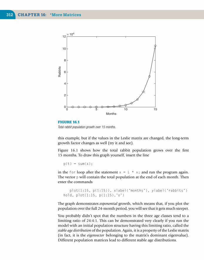
312 CHAPTER 16: *More Matrices
12× 104
10
8
6
4
2
00 5 10
Months
Rab
bits
15
FIGURE 16.1Total rabbit population growth over 15 months.
this example, but if the values in the Leslie matrix are changed, the long-termgrowth factor changes as well (try it and see).
Figure 16.1 shows how the total rabbit population grows over the first15 months. To draw this graph yourself, insert the line
p(t) = sum(x);
in the for loop after the statement x = L * x; and run the program again.The vector p will contain the total population at the end of each month. Thenenter the commands
plot(1:15, p(1:15)), xlabel(’months’), ylabel(’rabbits’)hold, plot(1:15, p(1:15),’o’)
The graph demonstrates exponential growth, which means that, if you plot thepopulation over the full 24-month period, you will see that it gets much steeper.
You probably didn’t spot that the numbers in the three age classes tend to alimiting ratio of 24:4:1. This can be demonstrated very clearly if you run themodel with an initial population structure having this limiting ratio, called thestable age distribution of the population. Again, it is a property of the Leslie matrix(in fact, it is the eigenvector belonging to the matrix’s dominant eigenvalue).Different population matrices lead to different stable age distributions.

16.2 Markov Processes 313
The interesting point about this is that a given Leslie matrix always, eventually,gets a population into the same stable age distribution, which eventuallyincreases by the same growth factor each month, no matter what the initial pop-ulation breakdown is. For example, if you run the above model with any otherinitial population, it will always eventually move into a stable age distributionof 24:4:1 with a growth factor of 2 (try it and see).
See help eig if you are interested in using MATLAB to compute eigenvaluesand eigenvectors.
16.2 MARKOV PROCESSES
Often a process that we wish to model may be represented by a number ofpossible discrete (i.e., discontinuous) states that describe its outcome. For exam-ple, if we are flipping a coin, the outcome is adequately represented by thestates heads and tails (and nothing in between). If the process is random, as itis with coins, there is a certain probability of being in either of the states at agiven moment and also a probability of changing from one state to another.If the probability of moving from one state to another depends on the presentstate only, and not on any previous state, the process is called a Markov chain.The progress of the myopic sailor in Chapter 15 is an example. Markov chainsare used widely in such diverse fields as biology and economics, to namejust two.
16.2.1 A random walkThis example is a variation on the random walk simulation in Section 15.5.A short-sighted student wanders down a street that has six intersections. Hishome is at intersection 1, and his favorite Internet cafe is at intersection 6. Ateach intersection other than his home or the cafe, he moves in the direction ofthe cafe with probability 2/3 and in the direction of his home with probability1/3. In other words, he is twice as likely to move toward the cafe as toward hishome. He never wanders down a side street. If he reaches his home or the cafe,he disappears into it, never to reappear (when he disappears we say in Markovjargon that he has been absorbed).
We would like to know the chances of the student ending up at home or in thecafe if he starts at a given corner (other than home or the cafe, obviously). Hecan clearly be in one of six states, with respect to his random walk, which canbe labeled by the intersection number, where state 1 means Home and state6 means Cafe. We can represent the probabilities of being in these states by asix-component state vector X(t), where Xi(t) is the probability of him being atintersection i at moment t. The components of X(t) must sum to 1, since hehas to be in one of these states.

314 CHAPTER 16: *More Matrices
We can express this Markov process with the following transition probabilitymatrix, P, where the rows represent the next state (i.e., corner) and the columnsrepresent the present state:
Home 2 3 4 5 Cafe
Home 1 1/3 0 0 0 02 0 0 1/3 0 0 03 0 2/3 0 1/3 0 04 0 0 2/3 0 1/3 05 0 0 0 2/3 0 0
Cafe 0 0 0 0 2/3 1
The entries for Home–Home and Cafe–Cafe are both 1 because he stays therewith certainty.
Using the probability matrix P, we can work out the student’s chances of being,say, at intersection 3 at moment (t + 1) as
X3(t + 1) = 2/3X2(t) + 1/3X4(t).
To get to 3, he must have been at either 2 or 4, and his chances of moving fromthere are 2/3 and 1/3, respectively.
Mathematically, this is identical to the Leslie matrix. We can therefore form thenew state vector from the old one each time with a matrix equation:
X(t + 1) = P X(t)
If we suppose the student starts at intersection 2, the initial probabilities will be(0; 1; 0; 0; 0; 0). The Leslie matrix script may be adapted with very few changesto generate future states:
n = 6;P = zeros(n); % all elements set to zero
for i = 3:6P(i,i–1) = 2/3;P(i–2,i–1) = 1/3;
end
P(1,1) = 1;P(6,6) = 1;x = [0 1 0 0 0 0]’; % remember x must be a column vector!
for t = 1:50x = P * x;disp( [t x’] )
end

16.3 Linear Equations 315
The edited output is
Time Home 2 3 4 5 Cafe
1 0.3333 0 0.6667 0 0 02 0.3333 0.2222 0 0.4444 0 03 0.4074 0 0.2963 0 0.2963 04 0.4074 0.0988 0 0.2963 0 0.19755 0.4403 0 0.1646 0 0.1975 0.19756 0.4403 0.0549 0 0.1756 0 0.32927 0.4586 0 0.0951 0 0.1171 0.32928 0.4586 0.0317 0 0.1024 0 0.4073
...20 0.4829 0.0012 0 0.0040 0 0.5119
...40 0.4839 0.0000 0 0.0000 0 0.5161
...50 0.4839 0.0000 0 0.0000 0 0.5161
By running the program long enough, we find the limiting probabilities: Thestudent ends up at home about 48% of the time and at the cafe about 52% ofthe time. Perhaps this is a little surprising: From the transition probabilities,we might have expected him to get to the cafe rather more easily. It just goes toshow that you should never trust your intuition when it comes to statistics.
16.3 LINEAR EQUATIONS
A problem that often arises in scientific applications is the solution to a systemof linear equations:
3x + 2y − z = 10 (16.2)
−x + 3y + 2z = 5 (16.3)
x − y − z = −1 (16.4)
MATLAB was designed to solve a system like this directly and very easily, as weshall now see.
If we define the matrix of coefficiets, A, as
A = 3 2 −1
−1 3 21 −1 −1

316 CHAPTER 16: *More Matrices
and the vectors of unknowns, x, and the right-hand side, b, as
x = x
yz
, b =
10
5−1
we can write the above system of three equations in matrix form as
3 2 −1
−1 3 21 −1 −1
x
yz
=
10
5−1
or even more concisely as the single matrix equation
Ax = b (16.5)
The solution may then be written as
x = A−1b (16.6)
where A−1 is the matrix inverse of A (i.e., the matrix that, when multipliedby A, gives the identity matrix I).
16.3.1 MATLAB’s solutionTo see how MATLAB solves this system, first recall that the left division oper-ator \ may be used on scalars—i.e., scalar a\b is the same as scalar b/a.However, it can also be used on vectors and matrices to solve linear equa-tions. Enter the following statements on the command line to solve Equations(16.2)–(16.4):
A = [3 2 –1; –1 3 2; 1 –1 –1];b = [10 5 –1]’;x = A \ b
which should result in
x =–2.00005.0000–6.0000
In terms of our notation, this means that the solution is x = −2, y = 5, z = −6.
You can think of the matrix operation A\b as “b divided by A,” or as “the inverseof A multiplied by b,” which is essentially what Equation (16.6) means.

16.3 Linear Equations 317
You may be tempted to implement Equation (16.6) in MATLAB as follows:
x = inv(A) * b
since the function inv finds a matrix inverse directly. However, A\b is actuallymore accurate and efficient. See MATLAB Help: Functions—Alphabetical Listand click on inv.
16.3.2 The residualWhenever we solve a system of linear equations numerically, we need to havesome idea of how accurate the solution is. The first thing to check is the residual,defined as
r = A*x – b
where x is the result of the operation x = A\b. Theoretically, the residualr should be zero, since the expression A * x is supposed to be equal to b,according to Equation (16.5), which is the one we are trying to solve. In ourexample here the residual is (check it)
r =1.0e–015 *
00.88820.6661
This seems conclusive: All the elements of the residual are less than 10−15 inabsolute value. Unfortunately, there may still be problems lurking beneath thesurface, as we shall see shortly.
First, however, we look at a situation where the residual turns out to be farfrom zero.
16.3.3 Overdetermined systemsWhen we have more equations than unknowns, the system is called overdeter-mined:
x − y = 0
y = 2
x = 1
Surprisingly, perhaps, MATLAB gives a solution to such a system. If
A = [1 –1; 0 1; 1 0];b = [0 2 1]’;

318 CHAPTER 16: *More Matrices
the statement
x = A \ b
results in
x =1.33331.6667
The residual r = A*x – b is now
r =–0.3333–0.33330.3333
What happens in this case is that MATLAB produces the least squares best fit. Thisis the value of x that makes the magnitude of r as small as possible:
√r(1)2 + r(2)2 + r(3)3
You can compute this quantity (0.5774) with sqrt(r’ * r) orsqrt(sum(r .* r)). There is a nice example of fitting a decaying expo-nential function to data with a least squares fit in MATLAB Help: Mathematics:Matrices and Linear Algebra: Solving Linear Equations: OverdeterminedSystems.
16.3.4 Underdetermined systemsIf there are fewer equations than unknowns, the system is called underdeter-mined. In this case there are an infinite number of solutions; MATLAB will findone that has zeros for some of the unknowns. The equations in such a systemare the constraints in a linear programming problem.
16.3.5 Ill-conditioned systemsSometimes the coefficients of a system of equations are the results of an experi-ment and may be sensitive to error. We need in that case to know how sensitivethe solution is. As an example, consider
10x + 7y + 8z + 7w = 32
7x + 5y + 6z + 5w = 23
8x + 6y + 10z + 9w = 33
7x + 5y + 9z + 10w = 31

16.3 Linear Equations 319
Use matrix left division to show that the solution is x = y = z = w = 1. Theresidual is exactly zero (check it), and all seems well. However, if we changethe right-hand side constants to 32.1, 22.9, 32.9, and 31.1, the “solution”is now given by x = 6, y = −7.2, z = 2.9, w = −0.1. The residual is verysmall.
A system like this is ill conditioned, meaning that a small change in the coef-ficients leads to a large change in the solution. The MATLAB function rcondreturns the condition estimator, which tests for ill conditioning. If A is the coef-ficient matrix, rcond(A) will be close to zero if A is ill conditioned, but closeto 1 if it is well conditioned. In this example, the condition estimator is about2 × 10−4, which is close to zero.
Some authors suggest the rule of thumb that a matrix is ill conditioned if itsdeterminant is small compared to the entries in the matrix. In this case thedeterminant of A is 1 (check with the function det), which is about an orderof magnitude smaller than most of its entries.
16.3.6 Matrix divisionMatrix left division, A\B, is defined whenever B has as many rows as A. Thiscorresponds formally to inv(A)*B, although the result is obtained withoutcomputing the inverse explicitly. In general,
x = A \ B
is a solution to the system of equations defined by Ax = B.
If A is square, matrix left division is done using Gauss elimination. If A is notsquare, the over- or underdetermined equations are solved in the least squaressense. The result is an m × n matrix X, where m is the number of columns of Aand n is the number of columns of B.
Matrix right division, B/A, is defined in terms of matrix left division such thatB/A is the same as (A’\B’)’. With a and b defined as for Equations (16.2)–(16.4), this means that
x = (b’/a’)’
gives the same solution. Try it, and make sure you can see why.
Sometimes the least squares solutions computed by \ or / for over- or under-determined systems can cause surprises, since you can legally divide one vectorby another. For example, if
a = [1 2];b = [3 4];

320 CHAPTER 16: *More Matrices
the statement
a / b
results in
ans =0.4400
This is because a/b is the same as (b’\a’)’, which is formally the solutionof b′ x′ = a′. The result is a scalar since a’ and b’ each have one column. Theresult is the least squares solution of
(34
)x =
(12
)
With this under your belt, can you explain why
a \ b
gives
ans =0 0
1.5000 2.0000
(try writing the equations out in full).
A complete discussion of the algorithms used in solving simultaneous linearequations may be found in MATLAB: Reference: MATLAB Function Reference:Alphabetical List of Functions: Arithmetic Operators + – * / \ ˆ ’.
16.4 SPARSE MATRICES
Matrices can sometimes have thousands of entries. Very large matrices canoccupy huge amounts of memory, and processing them can take up a lot of com-puter time. For example, a system of n simultaneous linear equations requiresn2 matrix entries, and the computing time to solve them is proportional to n3.
However, some matrices have relatively few nonzero entries. These are calledsparse as opposed to full. MATLAB has facilities for exploiting sparsity that havethe potential for saving huge amounts of memory and processing time. Forexample, the matrix representation of a certain type of partial differential equa-tion (a 5-point Laplacian) on a square 64 × 64 grid is a 4096 × 4096–elementmatrix with 20,224 nonzero elements. Its sparse form in MATLAB occupies

16.4 Sparse Matrices 321
only 250 kB of memory, whereas its full version occupies 128 MB, which iswell beyond the limits of most desktop computers. The solution to the systemAx = b using sparse techniques is about 4000 times faster than solving the fullcase—10 seconds instead of 12 hours!
In this section (which you can safely skip), we will look briefly at how to createsparse matrices in MATLAB. For a full description of sparse matrix techniquesconsult MATLAB Help: Mathematics: Sparse Matrices.
First an example, then an explanation. The transition probability matrix for therandom walk problem in Section 16.2 is a good candidate for sparse represen-tation. Only ten of its 36 elements are nonzero. Since the nonzeros appear onlyon the diagonal and the sub- and super-diagonals, a matrix representing moreintersections would be even sparser. For example, a 100 × 100 representationof the same problem would have only 198 nonzero entries (1.98%).
To represent a sparse matrix all that MATLAB needs to record are the nonzeroentries with their row and column indices. This is done with the sparse func-tion. The transition matrix of Section 16.2 can be set up as a sparse matrix withthe statements
n = 6;P = sparse(1, 1, 1, n, n);P = P + sparse(n, n, 1, n, n);P = P + sparse(1:n–2, 2:n–1, 1/3, n, n);P = P + sparse(3:n, 2:n–1, 2/3, n, n)
which (with format rat) result in
P =
(1,1) 1(1,2) 1/3(3,2) 2/3(2,3) 1/3(4,3) 2/3(3,4) 1/3(5,4) 2/3(4,5) 1/3(6,5) 2/3(6,6) 1
Each line of the display of a sparse matrix gives a nonzero entry with its rowand column (e.g., 2/3 in row 3 and column 2). To display a sparse matrix infull form, use the function
full(P)

322 CHAPTER 16: *More Matrices
which (also with format rat) results in
ans =1 1/3 0 0 0 00 0 1/3 0 0 00 2/3 0 1/3 0 00 0 2/3 0 1/3 00 0 0 2/3 0 00 0 0 0 2/3 1
The form of the sparse function used here is
sparse(rows, cols, entries, m, n)
This generates an m × n sparse matrix with nonzero entries having subscripts(rows, cols) (which may be vectors). Thus, the statement
sparse(1:n–2, 2:n–1, 1/3, n, n);
(with n = 6) creates a 6 × 6 sparse matrix with 4 nonzero elements, being1/3s in rows 1–4 and columns 2–5 (most of the super-diagonal). Notethat repeated use of sparse produces a number of 6 × 6 matrices, whichmust be added together to give the final form. Sparsity is therefore pre-served by operations on sparse matrices. See Help for more details onsparse.
It is quite easy to test the efficiency of sparse matrices. Construct a (full) identitymatrix
a = eye(1000);
Determine the time it takes to compute aˆ2. Then take advantage of the sparse-ness of a, which is an ideal candidate for representation as a sparse matrix sinceonly 1000 of its 1 million elements are nonzero. It is represented in sparseform as
s = sparse(1:1000, 1:1000, 1, 1000, 1000);
Now check the time it takes to find aˆ2. Use tic and toc to find outhow much faster the computation is. The function full(a) returns thefull form of the sparse matrix a (without changing the sparse representa-tion of a itself). Conversely, sparse(a) returns the sparse form of the fullmatrix a.
The function spy provides a neat visualization of sparse matrices. Try it on P.Then enlarge P to about 50 × 50 and spy it.

Summary 323
SUMMARY
■ The matrix left division operator \ is used for solving systems of linearequations directly. Because the matrix division operators \ and / cansometimes produce surprising results with the least squares solutionmethod, you should always compute the residual when solving a system ofequations.
■ If you work with large matrices with relatively few nonzero entries, considerusing MATLAB’s sparse matrix facilities.
CHAPTER EXERCISES
16.1. Compute the limiting probabilities for the student in Section 16.2 when he starts ateach of the remaining intersections in turn, and confirm that the closer to the cafe hestarts, the more likely he is to end up there. Compute Pˆ50 directly. Can you see thelimiting probabilities in the first row?
16.2. Solve the equations
2x − y + z = 4
x + y + z = 3
3x − y − z = 1
using the left division operator. Check your solution by computing the residual. Alsocompute the determinant (det) and the condition estimator (rcond). What do youconclude?
16.3. This problem demonstrates ill conditioning (where small changes in the coefficientscause large changes in the solution). Use the left division operator to show that thesolution
x + 5.000y = 17.0
1.5x + 7.501y = 25.503
is x = 2, y = 3. Compute the residual.
Now change the term on the right-hand side of the second equation to 25.501,a changeof about one part in 12,000, and find the new solution and the residual. The solutionis completely different. Also try changing this term to 25.502, 25.504, and so on. If thecoefficients are subject to experimental errors, the solution is clearly meaningless. Usercond to find the condition estimator and det to compute the determinant. Do thesevalues confirm ill conditioning?
Another way to anticipate ill conditioning is to perform a sensitivity analysis on thecoefficients: Change them all in turn by the same small percentage, and observe theeffect this has on the solution.
(Continued)

324 CHAPTER 16: *More Matrices
16.4. Use sparse to represent the Leslie matrix in Section 16.1. Test your representationby projecting the rabbit population over 24 months.
16.5. An excellent programming exercise is to code a Gauss reduction directly with opera-tions on the rows of the augmented coefficient matrix. See if you can write a functionto solve the general system Ax = b:
x = mygauss(A, B)
Skillful use of the colon operator in the row operations can reduce the code to a fewlines. Test your solution on A and b with random entries as well as on the systems inSection 16.3 and Exercise 16.4. Check it with left division.

CHAPTER 17
*Introduction to Numerical Methods
The objective of this chapter is to introduce numerical methods for
■ Solving equations■ Evaluating definite integrals■ Solving systems of ordinary differential equations■ Solving a parabolic partial differential equation
A major use of computers is finding numerical solutions to mathematical prob-lems that do not have analytical solutions (i.e., solutions that may be written interms of polynomials and standard mathematical functions). In this chapter welook briefly at some areas where numerical methods have been highly developed,such as solving nonlinear and differential equations and evaluating integrals.
17.1 EQUATIONS
In this section we consider how to solve numerically equations in one unknown.The usual way of expressing the problem is to say that we want to solve theequation f (x) = 0 (i.e., we want to find its root). This process is also described asfinding the zeros of f (x). There is no general method for finding roots analyticallyfor an arbitrary f (x).
17.1.1 Newton’s methodNewton’s method, perhaps the easiest numerical method for solving equations,was introduced briefly in earlier chapters. It is iterative, meaning that it repeat-edly attempts to improve an estimate of the root. If xk is an approximation of
Copyright © 2010, Daniel T. Valentine. Published by Elsevier Ltd. All rights reserved.DOI: 10.1016/B978-0-12-374883-6.00017-5 325

326 CHAPTER 17: *Introduction to Numerical Methods
f (xk)
f 9(xk)
xk11 xk
Root
FIGURE 17.1Newton’s method.
the root, we can relate it to the next approximation xk+1 using the right-angletriangle in Figure 17.1:
f ′(xk) = f (xk) − 0xk − xk+1
where f ′(x) is df /dx. Solving for xk+1 gives
xk+1 = xk − f (xk)
f ′(xk)
Here is a structure plan to implement Newton’s method:
1. Input starting value x0 and required relative error e2. While relative error |(xk − xk−1)/xk | ≥ e, repeat up to, say, k = 20:
xk+1 = xk − f (xk )/f ′(xk )Print xk+1 and f (xk+1)
3. Stop
It is necessary to limit step 2 since the process may not converge.
A script using Newton’s method (without the subscript notation) to solvex3 + x − 3 = 0 appeared in Chapter 10. If you run it, you will see that the valuesof x converge rapidly to the root. As an exercise, try running the script withdifferent starting values of x0 to see whether the algorithm always converges.
Try finding a nonzero root of 2x = tan(x) using Newton’s method. You mighthave some trouble with this one. If you do, you will have discovered themethod’s one serious problem: It converges to a root only if the starting guessis “close enough.” Since “close enough” depends on the nature of f (x) and on

17.1 Equations 327
0.5
0
x
f(x
)
0 0.2 0.4 0.6 0.8 1 1.2 1.4
20.5
21
21.5
22
22.5
1
FIGURE 17.2f (x ) = 2x − tan(x ).
the root, it is easy to get into difficulties here. The only remedy is intelligent trialand error on the initial guess, which is made considerably easier by sketchingf (x) or plotting it with MATLAB (see Figure 17.2).
If Newton’s method fails to find a root, try the Bisection method, discussed inSection 17.1.2.
Complex rootsNewton’s method can also find complex roots, but only if the startingguess is complex. Use the script from Chapter 10 to find a complex root ofx2 + x + 1 = 0. Start with a complex value of 1 + i, say, for x, which givesthe following output (if you replace disp( [x f(x)] ) in the script withdisp( x )):
0.0769 + 0.6154i−0.5156 + 0.6320i−0.4932 + 0.9090i−0.4997 + 0.8670i−0.5000 + 0.8660i−0.5000 + 0.8660iZero found
Since complex roots occur in complex conjugate pairs, the other root is−0.5 − 0.866i.

328 CHAPTER 17: *Introduction to Numerical Methods
17.1.2 The Bisection methodConsider again the problem of solving the equation f (x) = 0, where
f (x) = x3 + x − 3
We attempt to find by inspection, or trial and error, two values of x (call themxL and xR) such that f (xL) and f (xR) have different signs—f (xL)f (xR) < 0. If wecan find two such values, the root must lie somewhere in the interval betweenthem since f (x) changes sign on it (see Figure 17.3). In this example, xL = 1and xR = 2 will do, since f (1) = −1 and f (2) = 7. In the Bisection method, weestimate the root by xM, where xM is the midpoint of the interval [xL, xR]:
xM = (xL + xR)/2 (17.1)
If f (xM) has the same sign as f (xL), as drawn in the figure, the root clearly liesbetween xM and xR. We must then redefine the left-hand end of the interval ashaving the value of xM—that is, we let the new value of xL be xM. Otherwise, iff (xM) and f (xL) have different signs, we let the new value of xR be xM since theroot must lie between xL and xM in that case. Having redefined xL or xR, as thecase may be, we bisect the new interval again according to Equation (17.1) andrepeat the process until the distance between xL and xR is as small as we please.
The great advantage to this method is that before starting we can calculate howmany bisections are needed to obtain a certain accuracy, given initial values ofxL and xR. Suppose we start with xL = a and xR = b. After the first bisection, theworst possible error (E1) in xM is E1 = |a − b|/2, since we are estimating the
xM xR
f (x )
xL
FIGURE 17.3Bisection method.

17.1 Equations 329
root as being at the midpoint of the interval [a, b]. The worst that can happen isthat the root is actually at xL or xR, in which case the error is E1. Continuing likethis, after n bisections the worst possible error En is given by En = |a − b|/2n. Ifwe want to be sure that this is less than some specified error E, we must see toit that n satisfies the inequality |a − b|/2n < E:
n >log(|a − b|/E)
log(2)(17.2)
Since n is the number of bisections, it must be an integer. The smallest integern that exceeds the right-hand side of Inequality (17.2) will do as the maximumnumber of bisections required to guarantee the given accuracy E.
The following scheme may be used to program the Bisection method. It willwork for any function f (x) that changes sign (in either direction) between thetwo values a and b, which must be found beforehand by the user.
1. Input a, b, and E2. Initialize xL and xR3. Compute maximum bisections n from Inequality (17.2)4. Repeat n times:
Compute xM according to Equation (17.1)If f (xL) f (xM ) > 0 then
Let xL = xMotherwise
Let xR = xM5. Display root xM6. Stop
We assume that the procedure will not find the root exactly; the chances of thishappening with real variables are infinitesimal.
The main advantage of the Bisection method is that it is guaranteed to find aroot if you can find two starting values for xL and xR between which the func-tion changes sign. Also, you can compute in advance the number of bisectionsneeded to attain a given accuracy. Compared to Newton’s method, however,bisection is inefficient, as successive bisections do not necessarily move closerto the root, as usually happens with Newton’s. In fact, it is interesting to com-pare the two on the same function to see how many more steps the Bisectionmethod requires. For example, to solve the equation x3 + x − 3 = 0, the formertakes 21 steps to reach the same accuracy that the latter achieves in five steps.
17.1.3 The fzero and roots functionsThe MATLAB function fzero(@f, a) finds the zero nearest to the value a of thefunction f represented by the function f.m. Use it to find a zero of x3 + x − 3.fzero doesn’t appear to be able to find complex roots.

330 CHAPTER 17: *Introduction to Numerical Methods
The MATLAB function M-file roots(c) finds all the roots (zeros) of thepolynomial with coefficients in the vector c. (See Help for details.) Use it tofind a zero of x3 + x − 3.
17.2 INTEGRATION
Although most “respectable” mathematical functions can be differentiatedanalytically, the same cannot be said for integration. There are no general rulesfor integrating as there are for differentiating. For example, the indefinite inte-gral of a function as simple as e−x2
cannot be found analytically. We thereforeneed numerical methods, which is actually quite easy and depends on the factthat the definite integral of a function f (x) between the limits x = a and x = bis equal to the area under f (x) bounded by the x-axis and the two vertical linesx = a and x = b. Thus, all numerical methods for integrating simply involvemore or less ingenious ways of estimating the area under f (x).
17.2.1 The Trapezoidal ruleThe Trapezoidal (or Trapezium) rule is fairly simple to program. The area underf (x) is divided into vertical panels, each of width h (the step-length). If thereare n such panels, then nh = b − a—that is, n = (b − a)/h. If we join the pointswhere successive panels cut f (x), we can estimate the area under f (x) as thesum of the area of the resulting trapezia (see Figure 17.4). If we call thisapproximation to the integral S, then
S = h2
[f (a) + f (b) + 2
n−1∑i=1
f (xi)
], (17.3)
xi
f (x)
xi11
h
FIGURE 17.4Trapezoidal rule.

17.2 Integration 331
where xi = a + ih. Equation (17.3), the Trapezoidal rule, provides an estimatefor the integral
b∫a
f (x) dx.
Here is a function to implement the Trapezoidal rule:
function y = trap( fn, a, b, h )n = (b–a)/h;x = a + [1:n–1]*h;y = sum(feval(fn, x));y = h/2*(feval(fn, a) + feval(fn, b) + 2*y);
Note the following:
■ Since the summation in the rule is implemented with a vectorizedformula rather than a for loop (to save time), the function to beintegrated must use array operators where appropriate in its M-fileimplementation.
■ The user must choose h in such a way that the number of steps nwill be an integer—a check for this can be built in.
As an exercise, integrate f (x) = x3 between the limits 0 and 4 (remember towrite x.ˆ3 in the function M-file). Call trap as follows:
s = trap(@f, 0, 4, h);
With h = 0.1 the estimate is 64.04, and with h = 0.01 it is 64.0004 (the exactintegral is 64). You will find that as h gets smaller the estimate becomes moreaccurate.
This example assumes that f (x) is a continuous function that may be evaluatedat any x. In practice, the function can be defined at discrete points supplied asthe results of an experiment. For example, the speed of an object v(t) might bemeasured every so many seconds, and the distance traveled might be estimatedas the area under the speed–time graph. In this case, trap will have to bechanged by replacingfnwith a vector of function values (this is left as an exercisefor the curious). Alternatively, you can use the MATLAB function interp1 tointerpolate the data. (See Help).
17.2.2 Simpson’s ruleSimpson’s rule as a method of numerical integration is a good deal moreaccurate than the Trapezoidal rule and should always be used before you tryanything fancier. It too divides the area under the function to be integrated,
332 CHAPTER 17: *Introduction to Numerical Methods
f (x), into vertical strips, but instead of joining the points f (xi) with straight lines,every set of three such successive points is fitted with a parabola. To ensure thatthere is always an even number of panels, the step-length h is usually chosenso that there are 2n panels (i.e., n = (b − a)/(2h)).
Using the same notation as above, Simpson’s rule estimates the integral as
S = h3
[f (a) + f (b) + 2
n−1∑i=1
f (x2i) + 4n∑
i=1
f (x2i−1)
](17.4)
Coding this formula into a function M-file is left as an exercise.
If you try Simpson’s rule on f (x) = x3 between any limits, you will find, to yoursurprise, that it gives the same result as the exact mathematical solution. This isan extra benefit of the rule: It integrates cubic polynomials exactly (which canbe proved).
17.2.3 The quad functionNot surprisingly, MATLAB has a function, quad, to carry out numericalintegration, or quadrature, as it is also called. (See Help.)
17.3 NUMERICAL DIFFERENTIATION
The Newton quotient for a function f (x) is given by
f (x + h) − f (x)h
(17.5)
where h is “small.” As h tends to zero, this quotient approaches the first deriva-tive, df /dx. The Newton quotient may therefore be used to estimate a derivativenumerically. A useful exercise is to do this with a few functions for which youknow the derivatives. This way you can see how small you can make h beforerounding errors cause problems. Such errors arise because Expression (17.5)involves subtracting two terms that eventually become equal when the limit ofthe computer’s accuracy is reached.
As an example, the following script uses the Newton quotient to estimate f ′(x)for f (x) = x2 (which must be supplied as a function file f.m) at x = 2, forsmaller and smaller values of h (the exact answer is 4).
h = 1;x = 2;format short e

17.3 Numerical Differentiation 333
for i = 1:20nq = (f(x+h) – f(x))/h;disp( [h nq] )h = h / 10;
end
The output is:
1 51.0000e–001 4.1000e+0001.0000e–002 4.0100e+0001.0000e–003 4.0010e+0001.0000e–004 4.0001e+0001.0000e–005 4.0000e+0001.0000e–006 4.0000e+0001.0000e–007 4.0000e+0001.0000e–008 4.0000e+0001.0000e–009 4.0000e+0001.0000e–010 4.0000e+0001.0000e–011 4.0000e+0001.0000e–012 4.0004e+0001.0000e–013 3.9968e+0001.0000e–014 4.0856e+0001.0000e–015 3.5527e+0001.0000e–016 0...
These results show that the best h for this particular problem is about 10−8.
Generally, the best h for a given problem can only be found by trial and error,and this is not a trivial exercise. The problem does not arise with numericalintegration because numbers are added to find the area, not subtracted.
17.3.1 The diff functionIf x is a row or column vector:
[x(1) x(2) ... x(n)]
the MATLAB function diff(x) returns a vector of differences between adjacentelements:
[x(2)–x(1) x(3)–x(2) ... x(n)–x(n–1)]
The output vector is one element shorter than the input vector.

334 CHAPTER 17: *Introduction to Numerical Methods
In certain problems, diff is helpful in finding approximate derivatives. Forexample, if x contains displacements of an object every h seconds, diff(x)/his its speed.
17.4 FIRST-ORDER DIFFERENTIAL EQUATIONS
The most interesting real-life situations that we may want to model, or representquantitatively, are usually those in which the variables change in time (e.g.,biological, electrical, or mechanical systems). If the changes are continuous, asystem can often be represented with equations involving the derivatives of thedependent variables. Such equations are referred to as differential. The frequentaim of modeling is to be able to write down a set of differential equations (DEs)that describe the system being studied as accurately as possible. Very few DEscan be solved analytically, so numerical methods are once again required. Weconsider the simplest one in this section: Euler’s (rhymes with “boiler”). Wealso consider briefly how to improve it.
17.4.1 Euler’s methodIn general we want to solve a first-order DE (strictly, an ordinary DE, or ODE)of the form
dy/dx = f (x, y), y(0) given
Euler’s method consists of numerically replacing dy/dx with its Newtonquotient so that the ODE becomes
y(x + h) − y(x)h
= f (x, y)
After a slight rearrangement of terms, we get
y(x + h) = y(x) + hf (x, y) (17.6)
Solving an ODE numerically is such an important and common problem inscience and engineering that it is worth introducing some general notation atthis point. Suppose we want to integrate the ODE over the interval x = a (a = 0usually) to x = b. We break this interval into m steps of length h, so
m = (b − a)/h
(this is the same as the notation used in the update process of Chapter 11, exceptthat dt has been replaced by the more general h).
For consistency with MATLAB’s subscript notation, if we define yi as y(xi)
(the Euler estimate at the beginning of step i), where xi = (i − 1)h, then

17.4 First-Order Differential Equations 335
yi+1 = y(x + h) at the end of step i. We can then replace Equation (17.6) bythe iterative scheme
yi+1 = yi + hf (xi, yi) (17.7)
where y1 = y(0).
17.4.2 Example: Bacteria colony growthSuppose a colony of 1000 bacteria is multiplying at the rate of r = 0.8 per hourper individual (i.e., an individual produces an average of 0.8 offspring everyhour). How many bacteria are there after 10 hours? Assuming that the colonygrows continuously and without restriction, we can model this growth withthe DE
dN/dt = rN, N(0) = 1000 (17.8)
where N(t) is the population size at time t. This process is called exponentialgrowth, and Equation (17.8) may be solved analytically to give the well-knownformula for it:
N(t) = N(0)ert
To solve Equation (17.8) numerically, we apply Euler’s algorithm to get
Ni+1 = Ni + rhNi (17.9)
where the initial value N1 = 1000.
It is very easy to program Euler’s method. The following script implementsEquation (17.9), taking h = 0.5. It also computes the exact solution forcomparison.
h = 0.5;r = 0.8;a = 0;b = 10;m = (b – a) / h;N = zeros(1, m+1);N(1) = 1000;t = a:h:b;
for i = 1:mN(i+1) = N(i) + r * h * N(i);
end
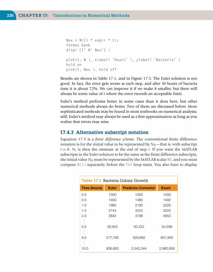
336 CHAPTER 17: *Introduction to Numerical Methods
Nex = N(1) * exp(r * t);format bankdisp( [t’ N’ Nex’] )
plot(t, N ), xlabel( ’Hours’ ), ylabel( ’Bacteria’ )hold onplot(t, Nex ), hold off
Results are shown in Table 17.1, and in Figure 17.5. The Euler solution is notgood. In fact, the error gets worse at each step, and after 10 hours of bacteriatime it is about 72%. We can improve it if we make h smaller, but there willalways be some value of t where the error exceeds an acceptable limit.
Euler’s method performs better in some cases than it does here, but othernumerical methods always do better. Two of them are discussed below. Moresophisticated methods may be found in most textbooks on numerical analysis;still, Euler’s method may always be used as a first approximation as long as yourealize that errors may arise.
17.4.3 Alternative subscript notationEquation 17.9 is a finite difference scheme. The conventional finite differencenotation is for the initial value to be represented by N0—that is, with subscripti = 0. Ni is then the estimate at the end of step i. If you want the MATLABsubscripts in the Euler solution to be the same as the finite difference subscripts,the initial value N0 must be represented by the MATLAB scalar N0, and you mustcompute N(1) separately, before the for loop starts. You also have to display
Table 17.1 Bacteria Colony Growth
Time (hours) Euler Predictor-Corrector Exact
0.0 1000 1000 1000
0.5 1400 1480 1492
1.0 1960 2190 2226
1.5 2744 3242 3320
2.0 3842 4798 4953...
5.0 28,925 50,422 54,598...
8.0 217,795 529,892 601,845...
10.0 836,683 2,542,344 2,980,958

17.4 First-Order Differential Equations 337
00
0.5
1
1.5
Bac
teria
2
2.5
31063
2 4 6Hours
8
(a)
(b)
10
FIGURE 17.5Bacteria colony growth: (a) Euler’s method; (b) exact solution.
or plot the initial values separately since they will no longer be included in theMATLAB vectors t, N, and Nex (which now have m instead of m + 1 elements).Here is a complete script to generate the Euler solution using finite differencesubscripts:
h = 0.5;r = 0.8;a = 0;b = 10;m = (b – a) / h;N = zeros(1, m); % one less element nowN0 = 1000;N(1) = N0 + r*h*N0; % no longer ’self-starting’
for i = 2:mN(i) = N(i–1) + r * h * N(i–1); %finite difference notation
end
t = a+h:h:b; % exclude initial time = aNex = N0 * exp(r * t);disp( [a N0 N0] ) % display initial values separatelydisp( [t’ N’ Nex’] )

338 CHAPTER 17: *Introduction to Numerical Methods
plot(a, N0) % plot initial values separatelyhold onplot(t, N ), xlabel( ’Hours’ ), ylabel( ’Bacteria’ )plot(t, Nex ), hold off
17.4.4 A predictor-corrector methodOne improvement on the numerical solution of the first-order DE
dy/dx = f (x, y), y(0) given
is as follows. The Euler approximation, which we are going to denote by anasterisk, is given by
y∗i+1 = yi + hf (xi, yi) (17.10)
but it favors the old value of y in computing f (xi, yi) on the right-hand side.Surely it would be better to say
y∗i+1 = yi + h
[f(xi+1, y∗
i+1) + f (xi, yi)
]/2 (17.11)
where xi+1 = xi + h, since this also involves the new value y∗i+1 in computing f
on the right-hand side. Of course, the problem is that y∗i+1 is as yet unknown, so
we can’t use it on the right-hand side of Equation (17.11). But we could use Eulerto estimate (predict) y∗
i+1 from Equation (17.10) and then use Equation (17.11)to correct the prediction by computing a better version of y∗
i+1, which we willcall yi+1. The full procedure is thus
Repeat as many times as required:Use Euler to predict: y∗
i+1 = yi + hf (xi , yi )Then correct y∗
i+1 to yi+1 = yi + h[ f (xi+1, y∗i+1) + f (xi , yi )]/2
This predictor-corrector method can easily be adapted to our problem. Therelevant lines of code are
for i = 1:m % m steps of length dtne(i+1) = ne(i) + r * h * ne(i);np = nc(i) + r * h * nc(i);nc(i+1) = nc(i) + r * h * (np + nc(i))/2;disp( [t(i+1) ne(i+1) nc(i+1) nex(i+1)] )
end;
ne stands for the “straight” (uncorrected) Euler solution; np is the Euler predic-tor (since this is an intermediate result, a vector is not needed for np); and ncis the corrector. The worst error is now only 15%, which is much better thanthe uncorrected Euler solution, although there is still room for improvement.

17.6 Runge-Kutta Methods 339
17.5 LINEAR ORDINARY DIFFERENTIALEQUATIONS
Linear ordinary differential equations (ODEs) with constant coefficients may besolved analytically in terms of matrix exponentials, which are represented in MAT-LAB by the function expm. For an example, see MATLAB Help: Mathematics:Matrices and Linear Algebra: Matrix Powers and Exponentials.
17.6 RUNGE-KUTTA METHODS
A variety of algorithms with the general name of Runge-Kutta can be used tointegrate systems of ODEs. The formulae involved are rather complicated; theycan be found in most books on numerical analysis.
However, as you may have guessed, MATLAB has plenty of ODE solvers, whichare discussed in MATLAB Help: Mathematics: Differential Equations. Amongthem are ode23 (second/third order) and ode45 (fourth/fifth order), whichimplement Runge-Kutta methods. (The order of a numerical method is thepower of h (i.e., dt) in the leading error term. Since h is generally very small, thehigher the power, the smaller the error.) We will demonstrate the use of ode23and ode45 here, first with a single first-order ODE and then with systems ofsuch equations.
17.6.1 A single differential equationHere’s how to use ode23 to solve the bacteria colony growth problem,Equation (17.8):
dN/dt = rN, N(0) = 1000
Step 1 Write a function file for the right-hand side of the DE to be solved.The function must have input variables t and N in this case (i.e.,independent and dependent variables of the DE), in that order. Createthe function file f.m as follows:
function y = f(t, Nr)y = 0.8 * Nr;
Step 2 Enter the following statements in the Command Window:
a = 0;b = 10;n0 = 1000;[t, Nr] = ode23(@f, [a:0.5:b], n0);

340 CHAPTER 17: *Introduction to Numerical Methods
Step 3 Note that the input arguments of ode23:■ @f is a handle for the function f, which contains the
right-hand side of the DE;
[a:0.5:b] is a vector (tspan) specifying the range ofintegration. If tspan has two elements ([a b]), the solverreturns the solution evaluated at every integration step (itchooses the integration steps and may vary them). This formis suitable for plotting. However, if you want to display thesolution at regular time intervals, as we want to here, use theform of tspan with three elements as above. The solution isthen returned evaluated at each time in tspan. The accuracyof the solution is not affected by the form of tspan used.
■ n0 is the initial value of the solution N.
Step 4 The output arguments are two vectors—that is, the solutions Nr attimes t. For 10 hours ode23 gives a value of 2,961,338 bacteria.From the exact solution in Table 17.1, we see that the error here isonly 0.7%.
If the solutions you get from ode23 are not accurate enough, you can requestgreater accuracy with an additional optional argument. (See Help.) If you needstill more accurate numerical solutions, you can use ode45 instead, which givesa final value of 2,981,290—an error of about 0.01%.
17.6.2 Systems of differential equations: ChaosThat weather prediction is so difficult and forecasts so erratic is no longerthought to be the result of complexity of the system but rather the result ofthe nature of the ODEs modeling it. These ODEs belong to a class referred to aschaotic; they produce wildly different results when their initial conditions arechanged infinitesimally. In other words, accurate weather prediction dependscrucially on the accuracy of the measurements of initial conditions.
Edward Lorenz, a research meteorologist, discovered this phenomenon in 1961.His original equations are far too complex to consider here, but the followingmuch simpler system has essentially the same chaotic features:
dx/dt = 10(y − x) (17.12)
dy/dt = −xz + 28x − y (17.13)
dz/dt = xy − 8z/3 (17.14)
This system may be solved very easily with MATLAB’s ODE solvers. The idea isto solve the ODEs with certain initial conditions, plot the solution, and thenchange the initial conditions very slightly and superimpose the new solutionover the old one to see how much it has changed.

17.6 Runge-Kutta Methods 341
We begin by solving the system with the initial conditions x(0) = −2,y(0) = −3.5 and z(0) = 21.
Step 1 Write a function file lorenz.m to represent the right-hand sides ofthe system as follows:
function f = lorenz(t, x)f = zeros(3,1);f(1) = 10 * (x(2) – x(1));f(2) = –x(1) * x(3) + 28 * x(1) – x(2);f(3) = x(1) * x(2) – 8 * x(3) / 3;
The three elements of the MATLAB vector x—x(1), x(2), and x(3)—respectively represent the three dependent scalar variables x, y, and z.The elements of the vector f represent the right-hand sides of thethree DEs. When a vector is returned by such a DE function, it mustbe a column vector—hence, the statement
f = zeros(3,1);
Step 2 Use the following commands to solve the system from, say, t = 0 tot = 10. Note that we use ode45 now, since it is more accurate.
x0 = [–2 –3.5 21]; % initial values in a vector[t, x] = ode45(@lorenz, [0 10], x0);plot(t,x)
You will see three graphs, for x, y, and z (in different colors).
Step 3 It is easier to see the effect of changing the initial values if there isonly one graph in the figure to start with. It is in fact best to plot thesolution y(t) on its own. The MATLAB solution x is actually a matrixwith three columns (as you can see from whos). The solution y(t)that we want will be the second column, so plot it by itself using thecommand
plot(t,x(:,2),’g’)
Then keep the graph on the axes with the command hold.
Now we can see the effect of changing the initial values. We just change theinitial value of x(0) from −2 to −2.04 (a change of only 2% and in only one ofthe three initial values). The following commands will do this, solve the ODEs,and plot the new graph of y(t) (in a different color):
x0 = [–2.04 –3.5 21];[t, x] = ode45(@lorenz, [0 10], x0);plot(t,x(:,2),’r’)

342 CHAPTER 17: *Introduction to Numerical Methods
230
220
210
0
Lore
nz s
olut
ions
y(t
)
10
20
30
t0 2 4 6 8 10
FIGURE 17.6Chaos?
Figure 17.6 shows that the two graphs are practically indistinguishable until t isabout 1.5. The discrepancy is gradual until t reaches about 6, when the solutionssuddenly and shockingly flip over in opposite directions. As t increases further,the new solution bears no resemblance to the old one.
Now solve the system (17.12)–(17.14) with the original initial values usingode23 this time:
x0 = [–2 –3.5 21];[t,x] = ode23(@lorenz, [0 10], x0);
Plot the graph of y(t) only—that is, x(:,2)—and then superimpose the ode45solution with the same initial values (in a different color). A strange thinghappens—the solutions begin to deviate wildly for t > 1.5. The initial con-ditions are the same; the only difference is the order of the Runge-Kuttamethod.
Finally solve the system with ode23s and superimpose the solution. (s standsfor “stiff.” For a stiff ODE, solutions can change on a very short time scale com-pared to the interval of integration.) The ode45 and ode23s solutions start todiverge only at t > 5. The explanation is that ode23, ode23s, and ode45 all havenumerical inaccuracies (if we could compare them with the exact solution—which incidentally can’t be found). However, the numerical inaccuracies aredifferent in the three cases and have the same effect as starting the numericalsolution with slightly different initial values.
How do we know when we have the “right” numerical solution? We don’t. Thebest we can do is increase the accuracy of the numerical method until no furtherwild changes occur over the interval of interest. In our example, then, we canonly be pretty sure of the solution for t < 5 (using ode23s or ode45). If that’snot good enough, we have to find a more accurate ODE solver.
Beware: chaotic DEs are very tricky to solve.

17.6 Runge-Kutta Methods 343
Incidentally, if you want to see the famous “butterfly” representation of chaos,just plot x against z as time increases (the resulting graph is called a phase planeplot). The following command will do the trick:
plot(x(:,1), x(:,3))
What you will see is a static 2-D projection of the trajectory, that is, the solutiondeveloping in time. Demos in the MATLAB Launch Pad includes an examplethat enables you to see the trajectory evolving dynamically in 3D (Demos:Graphics: Lorenz attractor animation).
17.6.3 Passing additional parameters to an ODE solverIn the examples of MATLAB ODE solvers, all of the coefficients on the right-handsides (e.g., the value 28 in Equation (17.13)) are constants. In a real modelingsituation, you will most likely want to change such coefficients frequently. Toavoid having to edit the function files each time you do so, pass the coefficientsas additional parameters to the ODE solver, which in turn passes them to theDE function. To see how this is done, consider the Lotka-Volterra predator-preymodel:
dx/dt = px − qxy (17.15)
dy/dt = rxy − sy (17.16)
where x(t) and y(t) are the prey and predator population sizes at time t, andp, q, r, and s are biologically determined parameters. For this example, we takep = 0.4, q = 0.04, r = 0.02, s = 2, x(0) = 105, and y(0) = 8.
First write a function M-file, volterra.m, as follows:
function f = volterra(t, x, p, q, r, s)f = zeros(2,1);f(1) = p*x(1) – q*x(1)*x(2);f(2) = r*x(1)*x(2) – s*x(2);
Then enter the following statements in the Command Window, which generatethe characteristically oscillating graphs in Figure 17.7:
p = 0.4; q = 0.04; r = 0.02; s = 2;[t,x] = ode23(@volterra,[0 10],[105; 8],[],p,q,r,s);plot(t, x)
Note that the additional parameters (p, q, r, and s) have to follow the fourthinput argument of the ODE solver, options (see Help). If no options have beenset (as in our case), use [] as a placeholder for the options parameter.

344 CHAPTER 17: *Introduction to Numerical Methods
0
20
40
60
80
100
Pop
ulat
ion
size
120
Time
(a)
(b)
0 2 4 6 8 10
FIGURE 17.7Lotka-Volterra model: (a) predator curve; (b) prey curve.
You can now change the coefficients from the Command Window and get anew solution, without editing the function file.
17.7 A PARTIAL DIFFERENTIAL EQUATION
The numerical solution to partial differential equations (PDEs) is a vast subjectbeyond the scope of this book. However, a class of PDEs called parabolic, oftenlead to solutions in terms of sparse matrices, which were mentioned briefly inChapter 16. One such example is considered in this section.
17.7.1 Heat conductionThe conduction of heat along a thin uniform rod may be modeled by the partialdifferential equation
∂u∂t
= ∂2u∂x2 (17.17)
where u(x, t) is the temperature distribution a distance x from one end of therod at time t, assuming that no heat is lost from the rod along its length.
Half the battle in solving PDEs is mastering the notation. We set up a rectangulargrid with step-lengths of h and k in the x and t directions, respectively. A generalpoint on the grid has coordinates xi = ih, yj = jk. A concise notation for u(x, t)at xi, yj is thus ui,j.

17.7 A Partial Differential Equation 345
Truncated Taylor series may then be used to approximate the PDE by a finitedifference scheme. The left-hand side of Equation (17.17) is usually approxi-mated by a forward difference:
∂u∂t
= ui,j+1 − ui,j
k
One way of approximating the right-hand side is by
∂2u∂x2 = ui+1,j − 2ui,j + ui−1,j
h2 (17.18)
This leads to a scheme that, although easy to compute, is only conditionallystable.
If we replace the right-hand side of the scheme in Equation (17.18) by the meanof the finite-difference approximation on the jth and ( j + 1)th time rows, we get(after a certain amount of algebra) the following scheme for Equation (17.17):
− rui−1,j+1 + (2 + 2r)ui,j+1 − rui+1,j+1 = rui−1,j + (2 − 2r)ui,j + rui+1,j
(17.19)
where r = k/h2. This is known as the Crank-Nicolson implicit method, since itinvolves solving a system of simultaneous equations, as we will see.
To illustrate the method numerically, let’s suppose that the rod has a length of1 unit and that its ends are in contact with blocks of ice—that is, the boundaryconditions are
u(0, t) = u(1, t) = 0 (17.20)
Suppose also that the initial temperature (initial condition) is
u(x, 0) ={
2x, 0 ≤ x ≤ 1/22(1 − x), 1/2 ≤ x ≤ 1
(17.21)
(This situation comes about by heating the center of the rod for a long time,with the ends kept in contact with the ice, and removing the heat source attime t = 0.) This particular problem has symmetry about the line x = 1/2; weexploit this now in finding the solution.
If we take h = 0.1 and k = 0.01, we have r = 1; Equation (17.19) becomes
− ui−1,j+1 + 4ui,j+1 − ui+1,j+1 = ui−1,j + ui+1,j (17.22)
Putting j = 0 in Equation (17.22) generates the following set of equationsfor the unknowns ui,1 (i.e., after one time step k) up to the midpoint of the

346 CHAPTER 17: *Introduction to Numerical Methods
rod, which is represented by i = 5 (x = ih = 0.5). The subscript j = 1 has beendropped for clarity:
0 + 4u1 − u2 = 0 + 0.4
−u1 + 4u2 − u3 = 0.2 + 0.6
−u2 + 4u3 − u4 = 0.4 + 0.8
−u3 + 4u4 − u5 = 0.6 + 1.0
−u4 + 4u5 − u6 = 0.8 + 0.8
Symmetry then allows us to replace u6 in the last equation with u4. Theseequations can be written in matrix form as
4 −1 0 0 0−1 4 −1 0 0
0 −1 4 −1 00 0 −1 4 −10 0 0 −2 4
u1
u2
u3
u4
u5
=
0.40.81.21.61.6
(17.23)
The matrix A on the left is referred to as tridiagonal. Having solved for ui,1 wecan then put j = 1 in Equation (17.22) and proceed to solve for the ui,2 and soon. The system (17.23) can of course be solved directly in MATLAB with the leftdivision operator. In the script below, the general form of Equations (17.23) istaken as
Av = g (17.24)
Care needs to be taken when constructing the matrix A. The following notationis often used:
A =
b1 c1
a2 b2 c2
a3 b3 c3
. . .
an−1 bn−1 cn−1
an bn
A is an example of a sparse matrix.
The script below implements the general Crank-Nicolson scheme of Equation(17.19) to solve this particular problem over 10 time steps of k = 0.01. Thestep-length is specified by h = 1/(2n) because of symmetry; r is therefore notrestricted to the value 1, although it takes this value here. The script exploits thesparsity of A by using the sparse function.

17.7 A Partial Differential Equation 347
format compactn = 5;k = 0.01;h = 1 / (2 * n); % symmetry assumedr = k / h ˆ 2;
% set up the (sparse) matrix Ab = sparse(1:n, 1:n, 2+2*r, n, n); % b(1) .. b(n)c = sparse(1:n–1, 2:n, –r, n, n); % c(1) .. c(n–1)a = sparse(2:n, 1:n–1, –r, n, n); % a(2) ..A = a + b + c;A(n, n–1) = –2 * r; % symmetry: a(n)full(A) %disp(’ ’)
u0 = 0; % boundary condition (Eq 19.20)u = 2*h*[1:n] % initial conditions (Eq 19.21)u(n+1) = u(n–1); % symmetrydisp([0 u(1:n)])
for t = k*[1:10]g = r * ([u0 u(1:n–1)] + u(2:n+1)) ...
+ (2 – 2 * r) * u(1:n); % Eq 19.19v = A\g’; % Eq 19.24disp([t v’])u(1:n) = v;u(n+1) = u(n–1); % symmetry
end
To preserve consistency between the formal subscripts of Equation (17.19) (andothers) and MATLAB subscripts, u0 (the boundary value) is represented by thescalar u0.
In the following output the first column is time and subsequent columns arethe solutions at intervals of h along the rod:
0 0.2000 0.4000 0.6000 0.8000 1.00000.0100 0.1989 0.3956 0.5834 0.7381 0.76910.0200 0.1936 0.3789 0.5397 0.6461 0.6921
...0.1000 0.0948 0.1803 0.2482 0.2918 0.3069
MATLAB has some built-in PDE solvers. See MATLAB Help: Mathematics:Differential Equations: Partial Differential Equations.

348 CHAPTER 17: *Introduction to Numerical Methods
0
10
20
30
40
50
60
70
80
90
100
y(x
)
0 20 40 60 80 100x
FIGURE 17.8Cubic polynomial fit.
17.8 OTHER NUMERICAL METHODS
The ODEs considered earlier in this chapter are all initial value problems. Forboundary value problem solvers, see MATLAB Help: Mathematics: DifferentialEquations: Boundary Value Problems for ODEs.
MATLAB has many functions for handling other numerical procedures, suchas curve fitting, correlation, interpolation, minimization, filtering and convo-lution, and (fast) Fourier transforms. Consult MATLAB Help: Mathematics:Polynomials and Interpolation and Data Analysis and Statistics.
To illustrate curve fitting, the following script enables you to plot data pointsinteractively. When you finish (i.e., when the x coordinates of your last twopoints differ by less than 2 in absolute value), a cubic polynomial is fitted anddrawn (see Figure 17.8).
% Interactive script to fit a cubic to data points
clfhold onaxis([0 100 0 100]);
diff = 10;xold = 68;i = 0;xp = zeros(1); % data pointsyp = zeros(1);

Summary 349
while diff > 2[a b] = ginput(1);diff = abs(a – xold);if diff > 2i = i + 1;xp(i) = a;yp(i) = b;xold = a;plot(a, b, ’ok’)
endend
p = polyfit(xp, yp, 3 );x = 0:0.1:xp(length(xp));y= p(1)*x.ˆ3 + p(2)*x.ˆ2 + p(3)*x + p(4);plot(x,y), title( ’cubic polynomial fit’), ...
ylabel(’y(x)’), xlabel(’x’)hold off
Polynomial fitting may also be done interactively in a figure window usingTools → Basic Fitting.
SUMMARY
■ A numerical method is an approximate computer method for solving amathematical problem that may have no analytical solution.
■ A numerical method is subject to rounding error in the computer solutionand truncation error, where an infinite mathematical process, such as takinga limit, is approximated by a finite process.
■ MATLAB has a large number of useful functions for handling numericalmethods.
(Continued)
CHAPTER EXERCISES
17.1. Use Newton’s method in a script to solve the following (you may have to experimentwith the starting values). Check all your answers with fzero. Check those involvingpolynomial equations with roots. Hint : use fplot to get an idea of where the rootsare—for example,
fplot(’xˆ3–8*xˆ2+17*x–10’, [0 3])

350 CHAPTER 17: *Introduction to Numerical Methods
The Zoom feature also helps. In the figure window select the Zoom In button(magnifying glass) and click on the part of the graph you want to magnify.(a) x 4 − x = 10 (two real roots and two complex roots)
(b) e−x = sin x (infinitely many roots)
(c) x 3 − 8x 2 + 17x − 10 = 0 (three real roots)
(d) log x = cos x
(e) x 4 − 5x 3 − 12x 2 + 76x − 79 = 0 (four real roots)
17.2. Use the Bisection method to find the square root of 2, taking 1 and 2 as initial val-ues of xL and xR . Continue bisecting until the maximum error is less than 0.05 (useInequality (17.2) from Section 17.1 to determine how many bisections are needed).
17.3. Use the Trapezoidal rule to evaluate∫ 4
0 x 2dx , using a step-length of h = 1.
17.4. A human population of 1000 at time t = 0 grows at a rate given by
dN /dt = aN
where a = 0.025 per person per year. Use Euler’s method to project the populationover the next 30 years, working in steps: h = 2 years, h = 1 year, and h = 0.5 year.Compare your answers with the exact mathematical solution.
17.5. Write a function file euler.m that starts with the line
function [t, n] = euler(a, b, dt)
and uses Euler’s method to solve the bacteria growth DE (17.8). Use it in a script tocompare the Euler solutions for dt = 0.5 and 0.05 with the exact solution. Try to getyour output to look like this:
time dt = 0.5 dt = 0.05 exact
0 1000.00 1000.00 1000.000.50 1400.00 1480.24 1491.821.00 1960.00 2191.12 2225.54...5.00 28925.47 50504.95 54598.15
17.6. The basic equation for modeling radioactive decay is
dx/dt = −rx
where x is the amount of the radioactive substance at time t and r is the decay rate.
Some radioactive substances decay into other radioactive substances, which decay inturn. For example, Strontium 92 (r1 = 0.256/hr) decays into Yttrium 92 (r2 = 0.127/hr),which decays into Zirconium. Write a pair of differential equations for Strontium andYttrium to describe what is happening.
Starting at t = 0 with 5 × 1026 atoms of Strontium 92 and none of Yttrium, use theRunge–Kutta method (ode23) to solve the equations up to t = 8 hours in steps of1/3 hr. Use Euler’s method for the same problem, and compare your results.
17.7. The population x (t ) of the springbok (a species of small gazelle) in Kruger National Parkin South Africa may be modeled by the equation
dx/dt = (r − bx sin at )x

Summary 351
where r , b, and a are constants. Write a program that reads values for r , b, and a,and initial values for x and t , and uses Euler’s method to compute the springbokpopulation at monthly intervals over a period of two years.
17.8. The luminous efficiency (ratio of the energy in the visible spectrum to the total energy)of a black body radiator may be expressed as a percentage by the formula
E = 64.77T −4
7×10⁻⁵∫4×10⁻⁵
x−5(
e1.432/Tx − 1)−1
dx
where T is the absolute temperature in degrees Kelvin; x is the wavelength in cm; andthe range of integration is over the visible spectrum.
Write a general function simp(fn, a, b, h) to implement Simpson’s rule as givenin Equation (17.4). Taking T = 3500◦K, use simp to compute E , first with 10 inter-vals (n = 5) and then with 20 intervals (n = 10); compare your results. (Answers:14.512725% for n = 5; 14.512667% for n = 10).
17.9. Van der Pol’s equation is a second-order nonlinear differential equation that may beexpressed as two first-order equations as follows:
dx1/dt = x2
dx2/dt = ε(
1 − x 21
)x2 − b2x1
The solution to this system has a stable limit cycle, which means that if you plot itsphase trajectory (x1 against x2) starting at any point in the positive x1-x2 plane, thetrajectory always moves continuously into the same closed loop. Use ode23 to solvethis system numerically for x1(0) = 0 and x2(0) = 1. Draw some phase trajectories forb = 1 and ε ranging between 0.01 and 1.0. Figure 17.9 shows you what to expect.
23 22
22
22.5
21.5
21
20.5
0
0.5
1
1.5
2
2.5
21 0 1 2 3
FIGURE 17.9Trajectory of Van der Pol’s equation.

APPENDIX A
Syntax: Quick Reference
In this appendix we offer examples of the MATLAB syntax most commonly usedin this book.
A.1 EXPRESSIONS
x = 2 ˆ (2 * 3) / 4;x = A \ b; % solution of linear equationsa == 0 & b < 0 % a equals 0 AND b less than 0a ˜= 4 | b > 0 % a not equal to 4 OR b greater than 0
A.2 FUNCTION M-FILES
function y=f(x) % save as f.m% comment for help
function [out1, out2] = plonk(in1, in2, in3) % save as plonk.m% Three input arguments, two outputs...
function junk % no input/output arguments; save as junk.m
[t, x] = ode45(@lorenz, [0 10], x0); % function handle with @
A.3 GRAPHICS
plot(x, y), grid % plots vector y against vector x on a grid
plot(x, y, ’b––’) % plots a blue dashed line
353
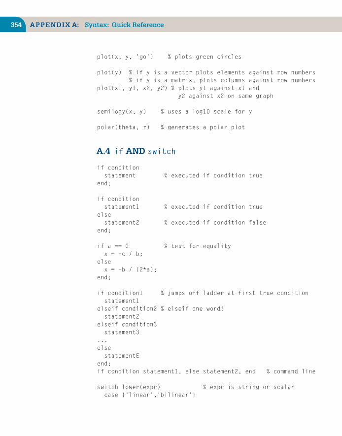
354 APPENDIX A: Syntax: Quick Reference
plot(x, y, ’go’) % plots green circles
plot(y) % if y is a vector plots elements against row numbers% if y is a matrix, plots columns against row numbers
plot(x1, y1, x2, y2) % plots y1 against x1 andy2 against x2 on same graph
semilogy(x, y) % uses a log10 scale for y
polar(theta, r) % generates a polar plot
A.4 if AND switch
if conditionstatement % executed if condition true
end;
if conditionstatement1 % executed if condition true
elsestatement2 % executed if condition false
end;
if a == 0 % test for equalityx = –c / b;
elsex = –b / (2*a);
end;
if condition1 % jumps off ladder at first true conditionstatement1
elseif condition2 % elseif one word!statement2
elseif condition3statement3
...elsestatementE
end;if condition statement1, else statement2, end % command line
switch lower(expr) % expr is string or scalarcase {’linear’,’bilinear’}

A.5 for and while 355
disp(’Method is linear’)case ’cubic’disp(’Method is cubic’)
case ’nearest’disp(’Method is nearest’)
otherwisedisp(’Unknown method.’)
end
A.5 for AND while
for i = 1:n % repeats statements n timesstatements
end;
for i = 1:3:8 % i takes values 1, 4, 7...
end;
for i = 5:–2:0 % i takes values 5, 3, 1...
end;
for i = v % index i takes on each element of vector vstatements
end;
for v = a % index v takes on each column of matrix astatements
end;
for i = 1:n, statements, end % command line version
try,statements,
catch,statements,
endwhile condition % repeats statements while condition is truestatements
end;
while condition statements, end % command line version

356 APPENDIX A: Syntax: Quick Reference
A.6 INPUT/OUTPUT
disp( x )
disp( ’Hello there’ )
disp([a b]) % two scalars on one line
disp([x’ y’]) % two columns (vectors x and ymust be same length)
disp( [’The answer is ’, num2str(x)] )
fprintf( ’\n’ ) % new line
fprintf( ’%5.1f\n’, 1.23 ) % **1.2
fprintf( ’%12.2e\n’, 0.123 ) % ***1.23e–001
fprintf( ’%4.0f and %7.2f\n’, 12.34, –5.6789 )
% **12 and **–5.68
fprintf( ’Answers are: %g %g\n’, x, y ) % matlab decides on format
fprintf( ’%10s\n’, str ) % left-justified string
x = input( ’Enter value of x: ’ )
name = input( ’Enter your name without apostrophes: ’, ’s’ )
A.7 load/save
load filename % retrieves all variablesfrom binary file filename.mat
load x.dat % imports matrix x from ASCII file x.datsave filename x y z % saves x y and z in filename.matsave % saves all workspace variables
in matlab.matsave filename x /ascii % saves x in filename (as ASCII file)

A.8 Vectors and Matrices 357
A.8 VECTORS AND MATRICES
a(3,:) % third row
a(:,2) % second column
v(1:2:9) % every second element from 1 to 9
v([2 4 5]) = [ ] % removes second, fourth and fifth elements
v(logical([0 1 0 1 0])) % second and fourth elements only
v’ % transpose
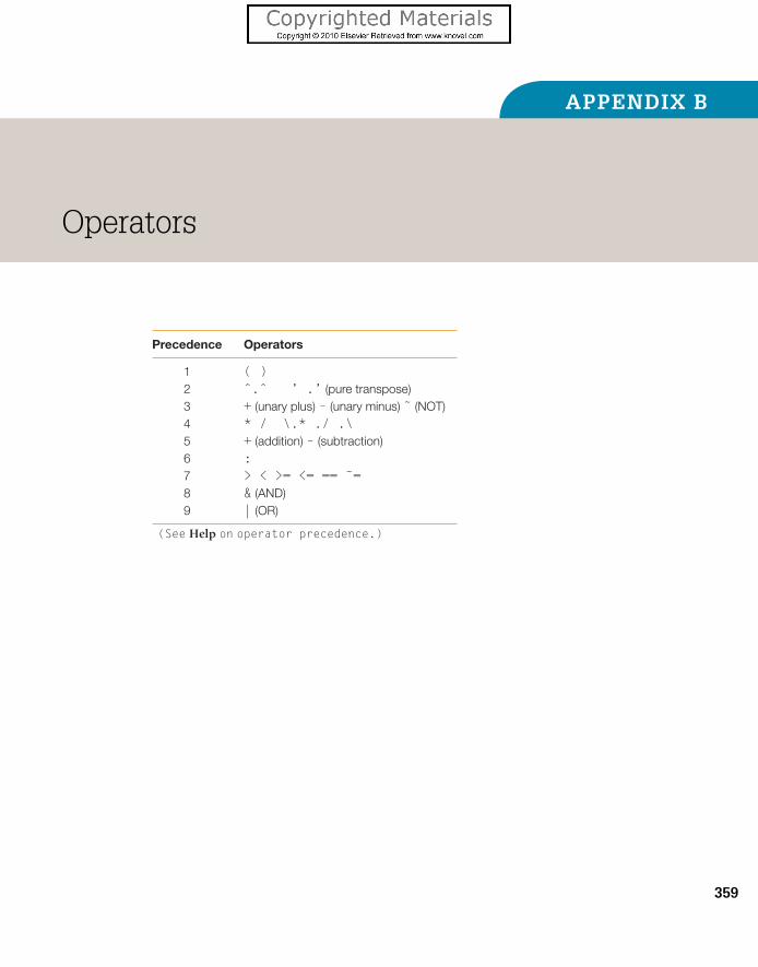
APPENDIX B
Operators
Precedence Operators
1 ( )2 ˆ.ˆ ’ .’ (pure transpose)3 + (unary plus) – (unary minus) ˜ (NOT)4 * / \.* ./ .\5 + (addition) – (subtraction)6 :7 > < >= <= == ˜=8 & (AND)9 | (OR)
(See Help on operator precedence.)
359

APPENDIX C
Command and Function: Quick Reference
This appendix lists most of the MATLAB commands and functions used in thetext, along with a few others. For a complete list by category (with links todetailed descriptions) see MATLAB: Reference: MATLAB Function Reference:Functions by Category in the online documentation.
The command help by itself displays a list of all the function categories (eachin its own directory).
C.1 GENERAL-PURPOSE COMMANDS
demo Run demoshelp Online helphelpwin Display categories of functions with links to each categorylookfor Keyword search through help entriestype List M-fileswhat Directory listing of M- and MAT-fileswhich Locate functions and files
C.1.1 Managing variables and the workspaceclear Clear variables and functions from memorydisp Display matrix or textlength Length of vectorload Retrieve variables from disksave Save workspace variables to disksize Array dimensionswho, whos List variables in workspace
C.1.2 Files and the operating systembeep Produce beep soundcd Change current working directory
361

362 APPENDIX C: Command and Function: Quick Reference
delete Delete filediary Save text of MATLAB sessiondir Directory listingedit Edit M-file! Execute operating system command
C.1.3 Controlling the Command Windowclc Clear Command Windowecho Echo commands in scriptformat Set output format for disphome Send cursor homemore Control paged output
C.1.4 Starting and quitting MATLABexit Terminate MATLABquit Terminate MATLABstartup Execute M-file when MATLAB starts
C.2 LOGICAL FUNCTIONS
all True if all elements of vector are true (nonzero)any True if any element of vector is trueexist Check if variable or file existsfind Find indices of nonzero elementsis* Detect various stateslogical Convert numeric values to logical values
C.3 MATLAB PROGRAMMING TOOLS
error Display error messageeval Interpret string containing MATLAB expressionfeval Function evaluationfor Repeat statement specific number of timesglobal Define global variableif Conditionally execute statementspersistent Define persistent variableswitch Switch among several casestry Begin try blockwhile Repeat statements conditionally

C.4 Matrices 363
C.3.1 Interactive inputinput Prompt user for inputkeyboard Invoke keyboard as script filemenu Generate menu of choices for user inputpause Wait for user response
C.4 MATRICES
eye Identity matrixlinspace Vector with linearly spaced elementsones Matrix of onesrand Uniformly distributed random numbers and arraysrandn Normally distributed random numbers and arrayszeros Matrix of zeros: (colon) Vector with regularly spaced elements
C.4.1 Special variables and constantsans Most recent answereps Floating-point relative accuracyi or j
√−1Inf InfinityNaN Not-a-Numbernargin, nargout Number of actual function argumentspi 3.14159 26535 897 . . .
realmax Largest positive floating-point numberrealmin Smallest positive floating-point numbervarargin, varargout Pass or return variable numbers of arguments
C.4.2 Time and datecalendar Calendarclock Wall clock (complete date and time)date Actual dateetime Elapsed timetic, toc Stopwatchweekday Day of week
C.4.3 Matrix manipulationcat Concatenate arraysdiag Create or extract diagonalfliplr Flip in left/right direction
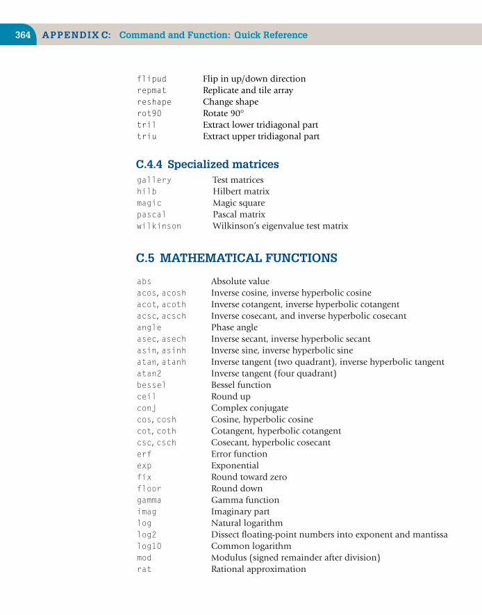
364 APPENDIX C: Command and Function: Quick Reference
flipud Flip in up/down directionrepmat Replicate and tile arrayreshape Change shaperot90 Rotate 90◦tril Extract lower tridiagonal parttriu Extract upper tridiagonal part
C.4.4 Specialized matricesgallery Test matriceshilb Hilbert matrixmagic Magic squarepascal Pascal matrixwilkinson Wilkinson’s eigenvalue test matrix
C.5 MATHEMATICAL FUNCTIONS
abs Absolute valueacos, acosh Inverse cosine, inverse hyperbolic cosineacot, acoth Inverse cotangent, inverse hyperbolic cotangentacsc, acsch Inverse cosecant, and inverse hyperbolic cosecantangle Phase angleasec, asech Inverse secant, inverse hyperbolic secantasin, asinh Inverse sine, inverse hyperbolic sineatan, atanh Inverse tangent (two quadrant), inverse hyperbolic tangentatan2 Inverse tangent (four quadrant)bessel Bessel functionceil Round upconj Complex conjugatecos, cosh Cosine, hyperbolic cosinecot, coth Cotangent, hyperbolic cotangentcsc, csch Cosecant, hyperbolic cosecanterf Error functionexp Exponentialfix Round toward zerofloor Round downgamma Gamma functionimag Imaginary partlog Natural logarithmlog2 Dissect floating-point numbers into exponent and mantissalog10 Common logarithmmod Modulus (signed remainder after division)rat Rational approximation

C.8 Polynomial Functions 365
real Real partrem Remainder after divisionround Round toward nearest integersec, sech Secant, hyperbolic secantsign Signum functionsin, sinh Sine, hyperbolic sinesqrt Square roottan, tanh Tangent, hyperbolic tangent
C.6 MATRIX FUNCTIONS
det Determinanteig Eigenvalues and eigenvectorsexpm Matrix exponentialinv Matrix inversepoly Characteristic polynomialrank Number of linearly independent rows or columnsrcond Condition estimatortrace Sum of diagonal elements{}\ and / Linear equation solution
C.7 DATA ANALYSIS
cumprod Cumulative productcumsum Cumulative sumdiff Difference functionfft One-dimensional fast Fourier transformmax Largest elementmean Average value of elementsmedian Median value of elementsmin Smallest elementprod Product of elementssort Sort in ascending orderstd Standard deviationsum Sum of elementstrapz Trapezoidal rule for numerical integration
C.8 POLYNOMIAL FUNCTIONS
polyfit Fit polynomial to datapolyval Evaluate polynomialroots Find polynomial roots

366 APPENDIX C: Command and Function: Quick Reference
C.9 FUNCTION FUNCTIONS
bvp4c Solve two-point boundary value problems for ODEsfmin Minimize function of one variablefmins Minimize function of several variablesfzero Find zero of function of one variableode23, ode23s,ode45 Solve initial value problems for ODEsquad Numerical integration
C.10 SPARSE MATRIX FUNCTIONS
full Convert sparse matrix to full matrixsparse Construct sparse matrix from nonzeros and subscriptsspy Visualize sparse matrix
C.11 CHARACTER STRING FUNCTIONS
char characters from ASCII codesdouble ASCII codes of characterslower Convert string to lower casesprintf Write formatted data to stringstr2mat String-to-matrix conversionstrcat String concatenationstrcmp Compare stringsupper Convert string to upper case
C.12 FILE I/O FUNCTIONS
fclose Close one or more open filesfeof Test for end-of-filefopen Open file or obtain information about open filesfprintf Write formatted data to filefread Read binary data from filefscanf Read formatted data from filefseek Set file position indicatorftell Get file position indicatorfwrite Write binary data to file
C.13 2D GRAPHICS
bar Bar graphgrid Grid lines

C.15 General 367
hist Histogram plotloglog Log-log scale plotplot Linear plotpolar Polar coordinate plotsemilogx Semi-log scale plotsemilogy Semi-log scale plottext Text annotationtitle Graph titlexlabel x-axis labelylabel y-axis labelzoom Zoom in and out on 2D plot
C.14 3D GRAPHICS
clabel Contour plot elevation labelcomet3 Animated 3D plotcontour Contour plot in 2Dcontour3 Contour plot in 3Dmesh 3D mesh surfacemeshc 3D mesh surface with contour plotmeshgrid X and Y arrays for 3D plotsplot3 Line plot in 3Dquiver Quiver plotsurf Shaded surfacesurfl Shaded surface with lightingview Rotation of 3D figurezlabel z-axis label
C.15 GENERAL
axes Create axes objectaxis Control axis scaling and appearancecla Clear axesclf Clear current figurecolorbar Display color bar (color scale)colormap Set color look-up table (list of colormaps)drawnow Complete any pending drawingfigure Create figure (graph) windowsfplot Plot functiongca Get current axes handlegcf Get current figure handlegco Return handle of current graphics object

368 APPENDIX C: Command and Function: Quick Reference
get Get graphics object propertiesginput Graphical input from mouse or cursorgtext Mouse placement of textset Set graphics object propertiessubplot Create axes in tiled positions

APPENDIX D
ASCII Character Codes
Code Char Code Char Code Char Code Char Code Char
0 (null) 26 → 52 4 78 N 104 h1 � 27 ← 53 5 79 O 105 i2 � 28 � 54 6 80 P 106 j3 ♥ 29 ↔ 55 7 81 Q 107 k4 ♦ 30 � 56 8 82 R 108 l5 ♣ 31 � 57 9 83 S 109 m6 ♠ 32 (blank) 58 : 84 T 110 n7 • 33 ! 59 ; 85 U 111 o8 34 ” 60 < 86 V 112 p9 ◦ 35 # 61 = 87 W 113 q10 36 $ 62 > 88 X 114 r11 � 37 % 63 ? 89 Y 115 s12 � 38 & 64 @ 90 Z 116 t13 � 39 ’ 65 A 91 [ 117 u14 40 ( 66 B 92 \ 118 v15 41 ) 67 C 93 ] 119 w16 � 42 ∗ 68 D 94 ˆ 120 x17 � 43 + 69 E 95 − 121 y18 � 44 , 70 F 96 ‘ 122 z19 !! 45 − 71 G 97 a 123 {20 ¶ 46 · 72 H 98 b 124 |21 § 47 / 73 I 99 c 125 }22 — 48 0 74 J 100 d 126 ∼23 � 49 1 75 K 101 e 127 �
24 ↑ 50 2 76 L 102 f25 ↓ 51 3 77 M 103 g
369
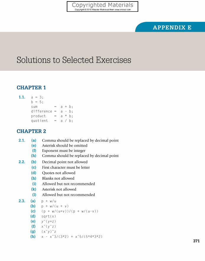
APPENDIX E
Solutions to Selected Exercises
CHAPTER 1
1.1. a = 3;b = 5;sum = a + b;difference = a – b;product = a * b;quotient = a / b;
CHAPTER 2
2.1. (a) Comma should be replaced by decimal point(e) Asterisk should be omitted(f) Exponent must be integer
(h) Comma should be replaced by decimal point
2.2. (b) Decimal point not allowed(c) First character must be letter(d) Quotes not allowed(h) Blanks not allowed(i) Allowed but not recommended(k) Asterisk not allowed(l) Allowed but not recommended
2.3. (a) p + w/u(b) p + w/(u + v)(c) (p + w/(u+v))/(p + w/(u–v))(d) sqrt(x)(e) yˆ(y+z)(f) xˆ(yˆz)(g) (xˆy)ˆz(h) x – xˆ3/(3*2) + xˆ5/(5*4*3*2)
371

372 APPENDIX E: Solutions to Selected Exercises
2.4. (a) i = i + 1
(b) i = iˆ3 + j
(c) if e > fg = e
elseg = f
end
(d) if d > 0x = –b
end
(e) x = (a + b)/(c * d)
2.5. (a) Expression not allowed on left-hand side(b) Left-hand side must be valid variable name(c) Left-hand side must be valid variable name
2.6. a = 2;b = –10;c = 12;x = (–b + sqrt(b ˆ 2 – 4 * a * c)) / (2 * a)
2.7. gallons = input(’Enter gallons: ’);pints = input(’Enter pints: ’);pints = pints + 8 * gallons;litres = pints / 1.76
2.8. distance = 528;litres = 46.23;kml = distance / litres;l100km = 100 / kml;disp( ’Distance Litres used km/L L/100km’ );disp( [distance litres kml l100km] );
2.9. t = a;a = b;b = t;
2.10. a = [a b]; % make ’a’ into a vectorb = a(1);a(1) = [];
2.11. (a) c = input(’Enter Celsius temperature: ’);f = 9 * c / 5 + 32;disp( [’The Fahrenheit temperature is:’ num2str(f)] );
(b) c = 20 : 30;f = 9 * c / 5 + 32;

APPENDIX E: Solutions to Selected Exercises 373
format bank;disp(’ Celsius Fahrenheit’);disp([c’ f’]);
2.12. degrees = 0 : 10 : 360;radians = degrees / 180 * pi;format bank;disp(’ Degrees Radians’);disp([degrees’ radians’]);
2.13. degrees = 0 : 30 : 360;radians = degrees / 180 * pi;sines = sin(radians);cosines = cos(radians);tans = tan(radians);table = [degrees’ sines’ cosines’ tans’]
2.14. for int = 10 : 20disp( [int sqrt(int)] );
end
2.15. sum(2 : 2 : 200)
2.16. m = [5 8 0 10 3 8 5 7 9 4];disp( mean(m) )
2.17. x = 2.0833, a = 4
2.18. % With for loopi = 1;x = 0;for a = i : i : 4x = x + i / a;
end
% With vectorsi = 1;a = i : i : 4;x = i ./ a;sum(x)
2.19. (b) n = input(’Number of terms? ’);k = 1 : n;s = 1 ./ (k .ˆ 2);disp(sqrt(6 * sum(s)))
2.21. r = 5;c = 10;l = 4;

374 APPENDIX E: Solutions to Selected Exercises
e = 2;w = 2;i = e / sqrt(r ˆ 2 + (2 * pi * w * l – 1 / (2 * pi * w * c)) ˆ 2)
2.22. con = [200 500 700 1000 1500];for units = conif units <= 500cost = 0.02 * units;
elseif units <= 1000cost = 10 + 0.05 * (units – 500);
elsecost = 35 + 0.1 * (units – 1000);
endcharge = 5 + cost;disp( charge )
end
2.24. money = 1000;for month = 1 : 12money = money * 1.01;
end
2.26. t = 1790 : 10 : 2000;p = 197273000 ./ (1 + exp(–0.03134 * (t – 1913.25)));disp([t’ p’]);pause;plot(t,p);
2.27. (a) r = 0.15;l = 50000;n = 20;
p = r * l * (1 + r / 12) ˆ (12 * n) / ...(12 * ((1 + r / 12) ˆ (12 * n) – 1))
2.28. (a) r = 0.15;l = 50000;p = 800;n = log(p / (p – r * l / 12)) / (12 * log(1 + r / 12))
CHAPTER 3
3.1. You should get a picture of tangents to a curve.3.2. (a) 4
(b) 2(c) Algorithm (attributed to Euclid) finds the HCF (highest common
factor) of two numbers using the fact that it divides exactly into

APPENDIX E: Solutions to Selected Exercises 375
the difference between the two numbers, and that, if the numbersare equal, they are equal to their HCF.
3.3. f = input(’Enter Fahrenheit temperature: ’);c = 5 / 9 * (f – 32);disp( [’The Celsius temperature is: ’ num2str(c)] );
3.4. a = input(’Enter first number: ’);b = input(’Enter second number: ’);if a < bdisp( [ num2str(b) ’ is larger.’] );
elseif a > bdisp( [ num2str(a) ’ is larger.’] );
elsedisp( ’Numbers are equal.’ );
end
3.6. 1. Input a, b, c, d, e, f2. u = ae – db, v = ec – bf3. If u = 0 and v = 0, then
Lines coincideOtherwise if u = 0 and v �= 0, then
Lines are parallelOtherwise
x = v/u, y = (af – dc)/uPrint x, y
4. Stop
a = input(’Enter a: ’);b = input(’Enter b: ’);c = input(’Enter c: ’);d = input(’Enter d: ’);e = input(’Enter e: ’);f = input(’Enter f: ’);u = a * e – b * d;v = c * e – b * f;if u == 0if v == 0disp(’Lines coincide.’);
elsedisp(’Lines are parallel.’);
endelsex = v / u;y = (a * f – d * c) / u;disp( [x y] );
end

376 APPENDIX E: Solutions to Selected Exercises
CHAPTER 4
4.2. (a) log(x + x ˆ 2 + a ˆ 2)(b) (exp(3 * t) + t ˆ 2 * sin(4 * t)) * (cos(3 * t)) ˆ 2(c) 4 * atan(1)(d) sec(x)ˆ2 + cot(x)(e) atan(a / x)
4.3. m = input(’Enter length in metres: ’);inches = m * 39.37;feet = fix(inches / 12);inches = rem(inches, 12);yards = fix(feet / 3);feet = rem(feet, 3);disp( [yards feet inches] );
4.5. a = 10;x = 1;k = input(’How many terms do you want? ’);for n = 1 : kx = a * x / n;if rem(n, 10) == 0disp( [n x] );
endend
4.6. secs = input(’Enter seconds: ’);mins = fix(secs / 60);secs = rem(secs, 60);hours = fix(mins / 60);mins = rem(mins, 60);disp( [hours mins secs] );
CHAPTER 5
5.2. (a) 1 1 0(b) 0 1 0(c) 1 0 1(d) 0 1 1(e) 1 1 1(f) 0 0 0(g) 0 2(h) 0 0 1
5.3. neg = sum(x < 0);pos = sum(x > 0);zero = sum(x == 0);

APPENDIX E: Solutions to Selected Exercises 377
5.7. units = [200 500 700 1000 1500];cost = 10 * (units > 500) + 25 * (units > 1000) + 5;cost = cost + 0.02 * (units <= 500) .* units;cost = cost + 0.05 * (units > 500 & units <= 1000) .* (units – 500);cost = cost + 0.1 * (units > 1000) .* (units – 1000);
CHAPTER 7
7.1. t = 1790:2000;P = 197273000 ./ (1+exp(–0.03134*(t–1913.25)));plot(t, P), hold, xlabel(’Year’), ylabel(’Population size’)census = [3929 5308 7240 9638 12866 17069 23192 31443 38558 ...
50156 62948 75995 91972 105711 122775 131669 150697];census = 1000 * census;plot(1790:10:1950, census, ’o’), hold off
7.2. a = 2;q = 1.25;th = 0:pi/40:5*pi;subplot(2,2,1)plot(a*th.*cos(th), a*th.*sin(th)), ...
title(’(a) Archimedes’) % or use polarsubplot(2,2,2)plot(a/2*q.ˆth.*cos(th), a/2*q.ˆth.*sin(th)), ...
title(’(b) Logarithmic’) % or use polar
7.4. n=1:1000;d = 137.51;th = pi*d*n/180;r = sqrt(n);plot(r.*cos(th), r.*sin(th), ’o’)
7.6. y(1) = 0.2;r = 3.738;for k = 1:600y(k+1) = r*y(k)*(1 – y(k));
endplot(y, ’.w’)
CHAPTER 8
8.1. balance = 1000;for years = 1 : 10for months = 1 : 12
balance = balance * 1.01;end
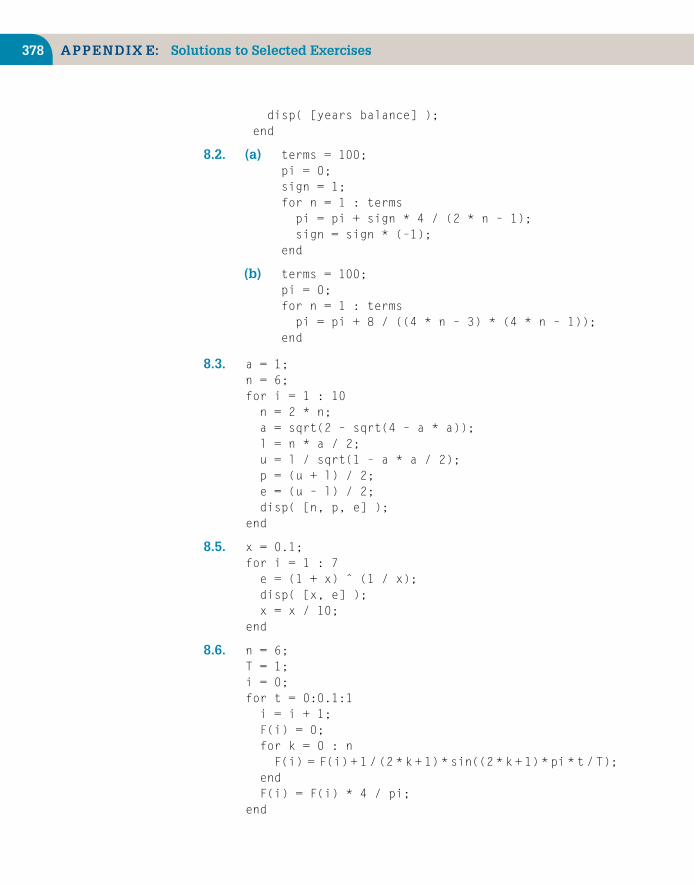
378 APPENDIX E: Solutions to Selected Exercises
disp( [years balance] );end
8.2. (a) terms = 100;pi = 0;sign = 1;for n = 1 : termspi = pi + sign * 4 / (2 * n – 1);sign = sign * (–1);
end
(b) terms = 100;pi = 0;for n = 1 : termspi = pi + 8 / ((4 * n – 3) * (4 * n – 1));
end
8.3. a = 1;n = 6;for i = 1 : 10n = 2 * n;a = sqrt(2 – sqrt(4 – a * a));l = n * a / 2;u = l / sqrt(1 – a * a / 2);p = (u + l) / 2;e = (u – l) / 2;disp( [n, p, e] );
end
8.5. x = 0.1;for i = 1 : 7e = (1 + x) ˆ (1 / x);disp( [x, e] );x = x / 10;
end
8.6. n = 6;T = 1;i = 0;for t = 0:0.1:1i = i + 1;F(i) = 0;for k = 0 : nF(i) = F(i) + 1 / (2 * k + 1) * sin((2 * k + 1) * pi * t / T);
endF(i) = F(i) * 4 / pi;
end

APPENDIX E: Solutions to Selected Exercises 379
t = 0:0.1:1;disp( [t’ F’] )plot(t, F)
8.8. sum = 0;terms = 0;while (sum + terms) <= 100terms = terms + 1;sum = sum + terms;
enddisp( [terms, sum] );
8.10. m = 44;n = 28;while m ~= nwhile m > n
m = m – n;endwhile n > m
n = n – m;end
enddisp(m);
CHAPTER 9
9.1. x = 2;h = 10;for i = 1 : 20h = h / 10;dx = ((x + h) ˆ 2 – x * x) / h;disp( [h, dx] );
end
CHAPTER 10
10.1. function pretty(n, ch)line = char(double(ch)*ones(1,n));disp(line)
10.2. function newquot(fn)x = 1;h = 1;for i = 1 : 10df = (feval(fn, x + h) – feval(fn, x)) / h;

380 APPENDIX E: Solutions to Selected Exercises
disp( [h, df] );h = h / 10;
end
10.3. function y = double(x)y = x * 2;
10.4. function [xout, yout] = swop(x, y)xout = y;yout = x;
10.6. % Script filefor i = 0 : 0.1 : 4disp( [i, phi(i)] );
end
% Function file phi.mfunction y = phi(x)a = 0.4361836;b = –0.1201676;c = 0.937298;r = exp(–0.5 * x * x) / sqrt(2 * pi);t = 1 / (1 + 0.3326 * x);y = 0.5 – r * (a * t + b * t * t + c * t ˆ 3);
10.8. function y = f(n)if n > 1y = f(n – 1) + f(n – 2);
elsey = 1;
end
CHAPTER 15
15.1. heads = rand(1, 50) < 0.5;tails = ∼heads;heads = heads * double(’H’);tails = tails * double(’T’);coins = char(heads + tails)
15.2. bingo = 1 : 99;for i = 1 : 99temp = bingo(i);swop = floor(rand * 99 + 1);bingo(i) = bingo(swop);bingo(swop) = temp;
end

APPENDIX E: Solutions to Selected Exercises 381
for i = 1 : 10 : 81disp(bingo(i : i + 9))
enddisp(bingo(91 : 99))
15.4. circle = 0;square = 1000;for i = 1 : squarex = 2 * rand – 1;y = 2 * rand – 1;if (x * x + y * y) < 1circle = circle + 1;
endenddisp( circle / square * 4 );
CHAPTER 16
16.5. function x = mygauss(a, b)n = length(a);
a(:,n+1) = b;
for k = 1:na(k,:) = a(k,:)/a(k,k); % pivot element must be 1
for i = 1:nif i ∼= ka(i,:) = a(i,:) – a(i,k) * a(k,:);
endend
end
% solution is in column n+1 of a:x = a(:,n+1);
CHAPTER 17
17.1. (a) Real roots at 1.856 and −1.697; complex roots at −0.0791 ±1.780i
(b) 0.589, 3.096, 6.285, … (roots get closer to multiples of π)
(c) 1, 2, 5

382 APPENDIX E: Solutions to Selected Exercises
(d) 1.303
(e) −3.997, 4.988, 2.241, 1.768
17.2. Successive bisections: 1.5, 1.25, 1.375, 1.4375, and 1.40625 (exactanswer: 1.414214 …, so the last bisection is within the required error)
17.3. 22 (exact answer: 21.3333)
17.4. After 30 years, exact answer: 2 117 (1000 ert)
17.6. The differential equations to be solved are
dS/dt = −r1S,
dY/dt = r1S − r2Y .
The exact solution after 8 hours is S = 6.450 × 1025 and Y = 2.312 ×1026.
17.8. function s = simp(f, a, b, h)x1 = a + 2 * h : 2 * h : b – 2 * h;sum1 = sum(feval(f, x1));x2 = a + h : 2 * h : b – h;sum2 = sum(feval(f, x2));s = h / 3 * (feval(f, a) + feval(f, b) + 2 * sum1 + 4 * sum2);
With 10 intervals (n = 5), luminous efficiency is 14.512725%. With 20intervals, it is 14.512667%. These results justify the use of 10 intervalsin any further computations. This is a standard way to test the accuracyof a numerical method: halve the step-length and see how much thesolution changes.
17.9. % Command Windowbeta = 1;ep = 0.5;[t, x] = ode45(@vdpol, [0 20], [0; 1], [], beta, ep);plot(x(:,1), x(:,2))
% Function file vdpol.mfunction f = vdpol(t, x, b, ep)f = zeros(2,1);f(1) = x(2);f(2) = ep * (1 – x(1)ˆ2) * x(2) – bˆ2 * x(1);

This page has been reformatted by Knovel to provide easier navigation.
INDEX
Index Terms Links
% 32
%e format specifier 64
%f format specifier 64
%g format specifier 64
& 113, 115 128
., 115
.* 36
./ 36
.ˆ 36
: 9 129
; 8 38
˜ 113
π 8
estimation of 306
0-1 vector 306
3-D plot 162
A
abs 62 92
acos 92
acosh 92
algorithm 78

Index Terms Links
This page has been reformatted by Knovel to provide easier navigation.
all 118 135
example 118
AND 113
angle 62
animation 253
comet3 163
ans 25 38
any 118
example 118
apostrophe 128
included in string 143
area 171
argument
input 208
input, pass by reference 214
input, pass by value 214
arithmetic operator 34
array 9 24
2-D 125
cell 240
multi-dimensional 140
string 144
Array Editor 25
array operation 36 136
ASCII code 144
asin 92
asinh 92
aspect ratio 62
assignment statement 38 66 241

Index Terms Links
This page has been reformatted by Knovel to provide easier navigation.
atan 92
atan2 62 92
atanh 92
axis 156
equal 62
normal 62
axis limits 156
azimuth 170
B
bacteria division 300
bacteria growth 306 335
balance delimiters 41
bar 171
bar graph 235
base workspace 212
best fit 318
binary to decimal conversion 151
binomial coefficient 185
Bisection method 328
bit 25
bitwise logical operations 113
blanks 146
break 188 194
breakpoint 219
Bubble Sort 236
bug 201
byte 25

Index Terms Links
This page has been reformatted by Knovel to provide easier navigation.
C
calendar 9
camel caps 24
cartesian co-ordinates 160
case 61
case sensitivity 24
catch 149
ceil 92
cell 240 241
cell array 240
celldisp 243
cellplot 243
Cervantes 151
chaos 182 255 340
butterfly 343
trajectory 343
char 145
cla 159
clc 9
clear 25
clear M-file 213
clf 159
clipboard 17
clock 51 92 267
colon operator 9 27 128
initialization 27
precedence 35
color 156

Index Terms Links
This page has been reformatted by Knovel to provide easier navigation.
colorbar 258
colormap 256
comet3 163
command 39
command line 7
command line editing 7
Command Window 5
command/function duality 217
comment 32
compass 172
compiler 20
complex conjugate transpose 62
complex numbers 61
concatenation of strings 144
condition estimator 319
conj 62
Contents.m 212
context menu 19
continuation of statement 32 38
continue 149 195
contour 165
contour plot 13
contour3 166
conversion, binary to decimal 151
cos 93
cosh 93
cot 93
Crank-Nicolson method 345
csc 93

Index Terms Links
This page has been reformatted by Knovel to provide easier navigation.
cumsum 93
current directory 15 19
Current Directory browser 19
curve fitting 348
cut and paste 17
D
data types 34
date 9 93
deal 240
deblank 146
Debugger 219
debugging 201
degrees to radians 8
del2 259
delimiter highlighting 41
demo 12
desktop 15
default 15
det 143
determinate repetition 185
diag 136
diary 30 103
dice 112
diff 333
differential equation 334
disp 42
scale factor 45
division, matrix 319

Index Terms Links
This page has been reformatted by Knovel to provide easier navigation.
docking 15
dot product 37
dot-transpose operator 115
double 34
double-precision 34
doubling time of an investment 190
drawnow 255
E
editing a plot 251
eig 143
eigenvalue 311
eigenvector 312
element-by-element operation 36
ellipse, equation of 181
ellipsis 32 38
elseif 57
empty 27
array 118
end 130
end of file 101
eps 109
error
fatal 201
logical 202
rounding 203
run-time 219
syntax 201
trapping 148

Index Terms Links
This page has been reformatted by Knovel to provide easier navigation.
errorbar 172
escape code 64
etime 51
Euler’s method 334
eval, error trapping 148
exclusive OR 113
exist 118
exp 93
explicit list, initializing vectors 26
expm 143 339
exponent 33
exponential fit 318
exponential growth 335
exponential matrix 339
exporting ASCII data, save 97
exporting binary data, save 97
expression 32 37
ans 38
display suppressed 38
evaluation 148
logical 53 113
response to input 66
eye 134
ezcontourf 173
F
factorial 47
false 107
feather 173

Index Terms Links
This page has been reformatted by Knovel to provide easier navigation.
feof 101
feval 216
Fibonacci numbers 225
field 238
fieldnames 239
figure 10 159
figure window 10 157
file I/O functions 65
file identifier 100
fill 174
find 118
findobj 249
finite difference scheme 336 345
fix 93
fixed point 33 44
fliplr 136
flipud 136
floating point 33 44
floor 49 93
fopen 100
for 48
command line version 50
common error 50
index 48
iteration count 49
more general 50
most general form 137
nested 138 188
replaced by vectorization 50

Index Terms Links
This page has been reformatted by Knovel to provide easier navigation.
for (cont.)
used for determinate loop 196
format 43 44
format specifiers 64
formula, vectorization 40
Fourier series 198
fplot 161
fprintf 63
escape code 64
string 146
fractal 182
fread 101
frequency distribution 235
fseek 102
ftell 103
full 322
full matrix 320
function 39 211
handle for passing as argument 216
help 212
MATLAB Function Reference 92
name resolution 218
P-code file 215
private 215
subfunction 215
function functions 217
function M-file 207
function/command duality 217
fzero 329

Index Terms Links
This page has been reformatted by Knovel to provide easier navigation.
G
Gauss reduction 130 (324 E)
Gaussian random number 305
gca 247
gcbo 267
gcf 246
gco 247
get 247
Gibbs phenomenon 198
ginput 159
global 212
gradient 167 168
graph 10
graphical user interface 263
graphics
2-D 153
3-D 162
3-D rotation 169
axis limits 156
contour plot 165
cropping a surface 167
easy-to-use commands 154
editing a plot 251
line type 156
logarithmic plot 159
mesh surface 163
multiple plots 155 157
on GUI 271

Index Terms Links
This page has been reformatted by Knovel to provide easier navigation.
graphics (cont.)
plotting symbol 156
polar co-ordinates 160
rapidly changing functions 161
saving 260
vector field 167
grid, on graph 155
gtext 155
guessing game 188
GUI 263
handles structure 270
plotting graph on 271
guide 263
H
H1 line 212
Halley’s comet 181
Handle Graphics objects 245
handle
function 216
graphics object 245
handles structure in a GUI 270
Help 15
help 12
Help browser 15
Help Navigator 92
help for a function 212
helpwin 91
hexadecimal 44

Index Terms Links
This page has been reformatted by Knovel to provide easier navigation.
hidden name 65 202 218
hist 175
histogram 235
hold 155
I
i 61
I/O functions 65
identity matrix 134
if 53
command line version 53
elseif 57
nested 59
vectorized with logical vector 119
if-else 55
command line 55
ill conditioning 319 323
imag 62
Import Wizard 98
importing ASCII data, load 97
importing binary data, load 98
importing data, Import
Wizard 98
inclusive OR 113
indeterminate repetition 185 188
index of for 48
Inf 7
infinity 7
initialization, colon operator 27
explicit list 26

Index Terms Links
This page has been reformatted by Knovel to provide easier navigation.
inline object 208
input 66
argument 208
string 143
vector 66
input argument 208
int2str 146
interpolation 331
interpreter 20
inv 143
ischar 147
isempty 118
isglobal 212
isinf 118
isnan 118
isothermal 165
iteration count 49
J
j 61
L
lasterr
error trapping 148
Launch Pad 12
least squares 318
left division 34 316 319
Legendre polynomial 225
length 94

Index Terms Links
This page has been reformatted by Knovel to provide easier navigation.
Leslie matrix 310
lighting 259
limit of sequence 47
line numbers 219
line style 156
linear equations
over-determined 317
residual 317
solution 315
under-determined 318
linspace 28
list, sorting 236
load 97
LODE 339
log 94
log10 94
logarithmic plot 159
logarithmic spiral 180
logical error 202
logical expression 53 107 113
vector 108
logical function 117
logical operator 57 113
precedence 114
logical vector 108
subscripting with 116
loglog 159
lookfor 12 212
loop
determinate 185

Index Terms Links
This page has been reformatted by Knovel to provide easier navigation.
loop (cont.)
indeterminate 188
Lorenz 340
Lotka-Volterra model 343
lower 147
lu 143
M
M-file 18
function 207
function passed as argument 216
macro 148
magic square 13 135
mantissa 33 44
marker 156
Markov chain 313
matrix 26 29 125
array operation 136
creating 127
deleting rows and columns 132
division 319
duplicating rows and columns 132
enlarging 128
exponential 339
exponentiation 142
full 320
Leslie 310
multiplication 140
operation 37 140

Index Terms Links
This page has been reformatted by Knovel to provide easier navigation.
matrix (cont.)
plot 153
sparse 320
subscript 127
transpose 29 128
visualization 168
max 94 238
mean 94
menu 195
mesh 164
mesh surface 163
meshc 166
meshgrid 163
meshz 175
Mexican hat 13
min 94 238
mlock 213
Monte Carlo estimation of π 306
more 43 193
multi-dimensional array 140
multiple lines in Command
Window 17
multiple plots 157
on same axes 155
munlock 213
N
name hiding 202 218
NaN 7

Index Terms Links
This page has been reformatted by Knovel to provide easier navigation.
nargin 214
nargout 214
nested fors 188
nested ifs 59
Newton quotient 204 224 332
Newton’s method 46
in general 325
normally distributed random number 305
NOT 113
not-a-number 7
num2str 43 146
number 33
numerical differentiation 332
numerical integration 330
numerical method 325
Bisection method 328
differential equation 334
differentiation 332
Euler’s method 334
integration 330
Newton quotient 332
Newton’s method 325
partial differential equation 344
predictor-corrector 338
Runge-Kutta method 339
Simpson’s rule 331
solution of equations 325
Trapezoidal rule 330
numerical solution
differential equations 334

Index Terms Links
This page has been reformatted by Knovel to provide easier navigation.
numerical solution (cont.)
equations 325
O
object 244
Handle Graphics 245
object-oriented programming 244
ones 133 145
operand 34
operating system, shelling out to 67
operation
array 36
element-by element 36
matrix 140
operator precedence, complete list 359
operator 114
arithmetic 34
colon 128
dot-transpose 115
left division 316
logical 57 113
precedence 34 114
relational 53
transpose 115
OR 113
exclusive 113
output 42
paging 43
suppressed with semi-colon 38
Index Terms Links
This page has been reformatted by Knovel to provide easier navigation.
output (cont.)
to a file with fprintf 64
output argument 210
over-determined system 317
P
P-code file 215
paging output 43
palindrome 151
partial differential equation 344
pascal 134
pause 170
pcode 215
peaks 170
persistent variable 212
pi 8
pie 176
pitfall 201
plot 153
3-D version 162
logarithmic scale 159
polar co-ordinates 160
plot edit mode 251
plot3 162
plotedit 251
plotyy 155
Poisson process 302
polar 160
polar co-ordinates 160

Index Terms Links
This page has been reformatted by Knovel to provide easier navigation.
polynomial fitting 349
pow2 94
pre-allocation 229
precedence 114
arithmetic operators 34
colon operator 35
logical operator 114
of operators, complete list 114 359
transpose 36
predator-prey model 343
predictor-corrector method 338
Preferences 44
prime number
largest known 192
test 191
private function 215
prod 94
Profiler 215
program 16
programming style 67
projectile motion 192
projectile trajectory 192
Property Editor 162
pseudo-code 85
pseudo-random number 94
Q
qr 143
quad 332
Index Terms Links
This page has been reformatted by Knovel to provide easier navigation.
quadratic equation 86
structure plan 86
quadrature 332
quiver 167
quote in string 43
R
radio-active decay 307
RAM 19
rand 94 111 133 297
seeding 298
uniform 297
randn 305
random access memory 19
random number 28 111
counting 111
generation 297
normal 305
uniform 297
random walk 235 300 313
rat 44
real 62
realmax 33 94
realmin 33 94
recall, smart 7
recursion 221
redimensioning 230
reference, pass by 214
relational operator 53
Index Terms Links
This page has been reformatted by Knovel to provide easier navigation.
relative accuracy 33
rem 94
removing elements of an array 29
repmat 132
reshape 131
reshaping a matrix 131
residual 317
ribbon 176
right division 319
rmfield 240
rolling dice 112
root of an equation 325
roots 268
rot90 136
round 113
rounding error 203 332
run-time error 219
Runge-Kutta method 339
S
save 97
saving a file 18
saving a graph 260
scalar 9
expansion 37
product 37
scientific notation 33
display 44
scope 212

Index Terms Links
This page has been reformatted by Knovel to provide easier navigation.
script file 18
hidden by variable of same
name 65
recommended way to run 19
search path 65
sec 31
seeding rand 298
semi-colon 8
semilogx 159
semilogy 159
sensitivity analysis 323
separator 39
series for π 197
set 248
Shakespeare 151
shelling out to the operating
system 67
sign 52
Simpson’s rule 331
simulation 113 235
bacteria division 300
bacteria growth 306
game of eights 307
π, estimation of 306
radio-active decay 307
random walk 300
rolling a die 299
spinning coins 298
traffic flow 302
Index Terms Links
This page has been reformatted by Knovel to provide easier navigation.
sin 8 39
single-precision 34
size 25 167
smart indenting 49
smart recall 7
sort 235 237
sort, bubble 236
sound 188
sparse 321 322 346
sparse matrix 320 346
spinning coins 298
spiral
Archimedes 180
logarithmic 180
sprintf 147
spy 169 322
sqrt 8
stable age distribution 312
stairs 177
statement 7 38 39
assignment 38
continuation 38
stem3 178
strcmp 146
string 43 125
array of characters 144
ASCII code 145
comparison 146

Index Terms Links
This page has been reformatted by Knovel to provide easier navigation.
string (cont.)
concatenation 144
containing quote 43
fprintf 146
including apostrophe 143
input 143
two-dimensional 147
struct 239
structure 238
structure plan 17 85
quadratic equation 86
structured programming 88
style 67
subfunction 215
subplot 157
subscript 28 127
logical vectors 116
out of range 128
vector 116
subscripting with logical vectors 116
sum 51 52 111
sunflower head 181
surf 164
surfc 166
svd 143
switch 60
syntax error 201
syntax highlighting 49

Index Terms Links
This page has been reformatted by Knovel to provide easier navigation.
T
tab completion 11
tan 11 110 154
tanh 284
Taylor series, exponential 224
text label on graph 155
text macro 148
tic 51
tiling 132
title 155
toc 51
top down programming 86
traffic flow 302
transpose 28 29 128
complex conjugate 62
precedence 36
Trapezoidal rule 330
tridiagonal matrix 346
tril 136
triu 136
true 107
truecolor 259
truncation error 349
try/catch 149
type 19
U
uicontrols 264
under-determined system 318

Index Terms Links
This page has been reformatted by Knovel to provide easier navigation.
undocking 15
unhiding a name 65
uniformly distributed random
number 297
update process 227
upper 147
V
value, pass by 214
Van der Pol’s equation 315
varargin 215 242
varargout 242
variable 7 20 23
global 212
hides script of same
name 65
persistent 212
scope 212
string 143
termed arrays by MATLAB 24
vector 9 26
0-1 306
colon operator 27
explicit list 26
incompatible sizes 202
input 66
pre-allocation 229
redimensioning 230
removing element 117

Index Terms Links
This page has been reformatted by Knovel to provide easier navigation.
vector (cont.)
scalar product 37
subscript 28 116
transpose 28
vectorization 40
instead of for 50
view 169
visualization of matrix 168
W
waterfall 178
while 189
command line form 190
used for indeterminate loop 196
vector condition 190
who 25
whos 25
why 14
workspace 24
base 212 214
function 25
Workspace Browser 25
X
xlabel 155
xor 113

Index Terms Links
This page has been reformatted by Knovel to provide easier navigation.
Y
ylabel 155
Z
Zeller’s congruence 151
zero of a function 325
zeros 133
zlabel 163
zoom 350