Essays on the Macroeconomics of Monetary Union

by

Anssi Rantala

Lic.Soc.Sc.

Academic dissertation to be presented, by the permission of the Faculty of Social Sciences of

the University of Helsinki, for public examination in Auditorium XV, Unioninkatu 34, on

January 30, 2004, at 1 p.m.

Helsinki 2004

Research Reports Kansantaloustieteen laitoksen tutkimuksia, No. 100:2004

Dissertationes Oeconomicae

ANSSI RANTALA

Essays on the Macroeconomics of Monetary Union

ISBN 952-10-1516-0 (nid.) ISBN 952-10-1515-2 (pdf)

Foreword The macroeconomics of EMU is an important and currently relatively intensively studied research topic. Anssi Rantala’s doctoral dissertation deals with two sets of issues by adopt-ing a game-theoretic approach to macroeconomic policy making: First, what is the impact of monetary unification on equilibrium unemployment in the presence of strategic wage setting, and second, how does the establishment of a monetary union affect the nominal wage flexibility and thereby unemployment fluctuations around the equilibrium unem-ployment rate? In the first essay the author shows that a switch from a flexible exchange rate regime to a monetary union will affect macroeconomic performance by falling unem-ployment if the degree of central bank conservatism in terms of the relative weight of infla-tion in central bank preferences is sufficiently high. The second essay studies the political economy of labour market flexibility in a monetary union by adopting a simple political economy approach, in which national governments decide on nominal wage flexibility, but face political costs, which increase with the chosen flexibility. Labour market policy coor-dination tends to increase the chosen level of nominal flexibility under discretionary monetary policy. The third essay provides a theoretical justification for establishing uniqueness of equilibrium in the model applied in the second essay by using the so-called adaptive learning approach of modelling private sector expectations. To conclude, this the-sis contributes to the emerging literature about the macroeconomics of EMU in several in-teresting ways. This study is part of the research agenda carried out by the Research Unit on Economic Structures and Growth (RUESG). The aim of RUESG is to conduct theoretical and empiri-cal research into important issues in the dynamics of the macro economy, game theory and economic organizations, the financial system as well as problems of labour markets, natural resources, taxation and econometrics. RUESG was established in the beginning of 1995 and it is now one of the National Centres of Excellence in research. RUESG is financed jointly by the Academy of Finland, the Uni-versity of Helsinki, the Yrjö Jahnsson Foundation, Bank of Finland and the Nokia Group. This support is gratefully acknowledged. Helsinki, December 16, 2003 Seppo Honkapohja Erkki Koskela Academy Professor Professor of Economics Co-Director Co-Director

Acknowledgements This thesis was written during the years 1999-2002, while I was working in the Research Unit on Economic Structures and Growth (RUESG) at the University of Helsinki. I am most grateful to the directors of the unit, Professors Seppo Honkapohja and Erkki Koskela, for giving me the opportunity to pursue my research interests and for their continuous sup-port and encouragement throughout the project. I also wish to thank my fellow researchers at RUESG for their friendship and sophisticated sense of humor. During the project I had the great opportunity to visit the Research Department of the Bank of Finland in 2000 and again in 2002-03. These two visits proved to be very important to the processing of research ideas, and I actually wrote the greater part of my thesis at the Bank. I would like to thank Head of Department Doctor Juha Tarkka for valuable sugges-tions concerning the essays and the Research Department for its hospitality and excellent working conditions. In particular, I am indebted to Docent Jouko Vilmunen for his enthusi-astic supervision and encouragement during the thesis project. I was fortunate to be able to spend the academic year 2001-02 at the Institute for Interna-tional Economic Studies at the University of Stockholm. I thank the Institute for its hospi-tality and support. A special note of thanks goes to Professor Lars Calmfors for many stimulating discussions about the EMU and labor market issues during my stay. Professor Mikko Puhakka and Docent Jouko Vilmunen acted as the official examiners of my thesis. They offered numerous constructive comments and suggestions to improve the contents of the manuscript, of which I wish to express my gratitude. I made the last revisions to the thesis while working at the Pellervo Economic Research Institute. I wish to thank my superiors, Doctors Raija Volk and Vesa Vihriälä for their flexibility and support at the final stages of the project. Financial support from the Yrjö Jahnsson Foundation and the Finnish Cultural Foundation is also gratefully acknowledged. Finally, I would like to thank my family and friends for bearing with me during this long project. I am very grateful to my parents, Kirsti and Risto Rantala, who have always sup-ported and encouraged me in my academic aspirations and in my life in general. Above all, I owe my deepest gratitude to my loved ones, my wife Maarit and our little princess Emma. Maarit’s seemingly endless love and unfaltering support have always inspired me and car-ried me through hard times in life. This thesis project could neither have been initiated nor, even more importantly, completed without her. Our precious daughter Emma is the greatest source of joy for me. Our days are always full of action with her. Even in the middle of the night one sometimes hears a voice asking “Isä, kerrotaanko mörköjuttuja?” I thank Maarit and Emma with all my heart for having taught me to realize how beautiful life is. Helsinki, December 18, 2003 Anssi Rantala

Contents Chapter 1 Introduction 1 Chapter 2 Strategic Wage Setting and Equilibrium Unemployment in a Monetary Union 11 Chapter 3 Labor Market Flexibility and Policy Coordination in a Monetary Union 49 Chapter 4 Adaptive Learning and Multiple Equilibria in a Natural Rate Model with Unemployment Persistence 97

Chapter 1

Introduction

1 Background

Monetary unification in Europe culminated in the launch of Euro banknotes and coins

in January 2002. A common currency among countries has, however, more wide-ranging

effects on the economies than the obvious benefits it brings along to travellers and business

firms by abolishing exchange commissions and exchange rate uncertainty. The arguments

related to the costs of a common currency are typically based on the theory of optimum

currency areas put forward by Mundell (1961) about forty years ago. The optimum

currency area approach focuses on the impact of asymmetric shocks and the necessary

adjustment mechanisms to counteract them. When countries have independent monetary

and exchange rate policies, the nominal exchange rate can, at least in principle, be used

to restore the labor market equilibrium after an asymmetric shock. If the countries have,

however, adopted a common currency, there are basically two alternative mechanisms,

which keep unemployment from rising in a country hit by an asymmetric negative shock;

either labor mobility between countries has to be considerable, or wages need to be

flexible. Needless to say that Europe seems to be a “Mundellian nightmare” with low

mobility of labor and inflexible wage structures.

The critics of the theory of optimum currency areas have pointed out that the ability of

exchange rate changes to absorb asymmetric shocks may be much weaker than the theory

suggests. Moreover, pure exchange rate shocks, that is, exchange rate movements not

driven by fundamentals, or even policy-induced exchange rate shocks are often considered

to be a source of macroeconomic disturbances. Giving up monetary independence can

then be welfare improving, provided that it decreases undesirable exchange rate volatility.

The most often mentioned economic benefits of a common currency are related to

increased international integration of financial and product markets. In particular, a

common currency is seen as a stimulus to international trade, which through more ef-

ficient resource allocation will increase per capita output and ultimately welfare. De

Grauwe (2000) offers a comprehensive treatment of both microeconomic and macroeco-

nomic aspects of monetary integration.

The standard cost-benefit analysis of the impact of monetary unification lacks an

important aspect. The formation of a monetary union is a fundamental regime change,

which could transform established behavioral relationships in the economy. Focusing on

labor markets, one can argue that the monetary regime will affect the constraints faced by

the labor unions and policy makers, and thereby the unemployment process may change

as well. Calmfors (2001b) provides a thorough survey and an assessment of the literature

on the relationship between monetary unification and wage bargaining institutions.

It is instructive to divide the impact of monetary unification on unemployment out-

comes through wage setting into two parts. The first part deals with the impact on the

equilibrium rate of unemployment. According to a conventional wisdom, money is just

a veil in the long run, and hence monetary regime will not affect equilibrium outcomes

in the real economy. However, it has been shown by e.g. Cukierman and Lippi (1999)

and Soskice and Iversen (2000) that assuming non-atomistic strategically behaving labor

unions will break the long-run neutrality so that the monetary policy strategy will affect

the real economy.1 The second part of the question is related to nominal wage flexibility

and cyclical sensitivity of unemployment around the equilibrium rate. The incentives for

reforms which increase nominal wage flexibility may change with monetary unification,

since the agents of the economy realize that the nominal exchange rate can’t anymore

be used to counteract the impact of asymmetric shocks. This has been studied by Sibert

and Sutherland (2000) and Calmfors (2001a).

A careful empirical assessment of the unemployment consequences of the European

Economic and Monetary Union, the EMU in short, will have to wait for some time.

In order to attain any reliable estimates of the impact, one should use long time series

containing several business cycles both before and after the establishment of the EMU.

Hence, while waiting for the data to accumulate, at this point theoretical work still

provides the only feasible way to conduct research on this topic.

This dissertation consists of three theoretical essays that contribute to the literature

on the macroeconomics of monetary union. The essays can be read independently of

each other. Since the topics of the essays are related, some repetition is unavoidable.

The first essay (Chapter 2) deals with the impact of monetary unification on equilibrium

1It is noteworthy that money will still be neutral in a sense that, other things equal, including thecentral bank’s behavior, changes in the nominal money stock will pass on to prices without affecting anyreal variables. See Soskice and Iversen (2000) for an illustration of this point.

2

unemployment. The second and the third essays (Chapters 3 and 4, respectively) are

related to nominal wage flexibility and unemployment fluctuations around the equilibrium

rate in a monetary union. The last two essays complement each other so that the third

essay provides a novel theoretical justification for establishing uniqueness of equilibrium

in the model applied in the second essay.

All three essays adopt a game-theoretic approach to macroeconomic policy making.

The central bank (or banks, as in the first essay) and labor unions are the players of the

game in each essay. In the second essay (Chapter 3) there are also national governments

involved. In the first and the second essays the main results are driven by strategic

interactions either between non-atomistic labor unions and the central bank (or banks),

or between national governments and the central bank. The third essay abstracts from

strategic behavior and focuses on the implications of adaptive learning on the stability

of rational expectations equilibria.

The modelling of central bank preferences adopted in this dissertation deviates from

the traditional practice in the literature on monetary policy games in one important

respect. The central bank is assumed to target the equilibrium rate of unemployment in-

stead of having an “over-ambitious” unemployment target which produces the celebrated

inflation bias result (see Barro and Gordon (1983)).2 The inflation bias model can be seen

as a rather good description of the incentives facing politicians when they are in charge

of monetary policy. If the natural rate is too high from the society’s point of view due to

e.g. imperfections in product and labor markets or distortionary taxation, governments

may be tempted to take the soft option and, instead of implementing politically costly

structural measures, try to use monetary policy to bring down unemployment. However,

when monetary policy is delegated to an independent central bank, there seems no rea-

son whatsoever for the central bank to target anything other than the natural rate (for

discussion on this point, see Blinder (1998)).

This monetary policy framework, where the central bank is concerned about keeping

inflation, and inflation expectations, low and stable and at the same time striving to limit

cyclical swings in resource utilization, has been referred to as constrained or enlightened

discretion (see e.g. Bernanke and Mishkin (1997) and Blinder (1998)). It can be said

that constrained discretion has become the standard approach to monetary policy in the

industrialized countries. In particular, the increasingly popular policy framework known

as inflation targeting can also be interpreted as constrained discretion rather than a strict

rule.

2To be precise, the model utilized in the second and the third essays makes a distinction between the“long-run” and the “short-run” natural rate of unemployment. In the baseline model the central banktargets the long-run natural rate. An extension considers also the short-run natural rate as a target.

3

Below follows brief summaries of the three essays in the order of their appearance.

2 Strategic Wage Setting and Equilibrium Unem-

ployment in a Monetary Union

The first essay (Chapter 2) investigates the impact of the formation of a monetary union

on equilibrium unemployment in the presence of strategic wage setting. According to

the natural rate hypothesis developed by Phelps (1967) and Friedman (1968), monetary

regime is neutral in the long run, and the equilibrium rate of unemployment is determined

only by real factors of the economy. The voluminous literature on monetary policy games

initiated by Kydland and Prescott (1977) and Barro and Gordon (1983) combines the

natural rate hypothesis with rational expectations and analyzes the optimal behavior of

the policy makers with well-known results. Only inflation depends systematically on the

conduct of monetary policy, and due to shocks in the economy unemployment fluctuates

around an exogenous natural rate. Hence, equilibrium unemployment should not be

affected by the establishment of a monetary union, which is just a change of monetary

regime.

Recent research by Grüner and Hefeker (1999) and Cukierman and Lippi (2001) sug-

gests, however, that in the presence of non-atomistic labor unions a non-neutrality result

of monetary unification emerges due to strategic interaction between labor unions and

monetary authorities. In particular, these contributions show that the establishment of

a monetary union will increase both unemployment and inflation, provided that national

labor unions are “inflation averse”. An inflation averse labor union refers to a one which

is, in addition to having traditional real wage and unemployment targets, also concerned

about inflation per se. Inflation aversion moderates wage claims and lowers unemploy-

ment under national monetary policy, because unions are willing to compromise over the

real wage target in order to reduce inflation. In a monetary union this moderating ef-

fect will be smaller and unemployment will rise. This argument, however, hinges on two

somewhat questionable assumptions; the existence of both inflation aversion and inflation

bias are crucial for the outcome. If either one is missing, monetary unification will have

no effect on unemployment.

In this essay, it is shown that in a model with open-economy spillovers, a switch from a

flexible exchange rate regime to a monetary union will affect macroeconomic performance,

even though national labor unions are not averse to inflation, and there is no inflation

bias. In particular, it is shown that unemployment will fall, provided that the degree of

central bank conservatism is sufficiently high, whereas with low degrees of conservatism

4

unemployment increases. Conservatism refers here to the relative weight of inflation in

the central bank preferences.

The mechanism behind the non-neutrality result is related to international spillovers

created by imperfect substitutability between goods produced in different countries. Due

to imperfect substitutability, the labor union’s wage claim will affect the real exchange

rate, which in turn influences consumer prices and real consumer wages. The strength of

the union’s ability to affect the real exchange rate depends on the monetary regime, and

under a flexible exchange rate also on the preferences of the monetary authorities toward

inflation and unemployment. Monetary regime will affect the labor union’s perceived real

wage—unemployment tradeoff through the real exchange rate channel. In other words, the

real consumer wage elasticity of labor demand is endogenous in the model. In this respect

the model is similar to Holden’s (2003) model with traded and non-traded sectors, where

the impact of monetary regime on wage setting is transmitted via labor demand elasticity.

Interestingly enough, relative to the flexible exchange rate regime, the inflexibility of the

common monetary policy in responding to a country specific wage increase is good news

in terms of unemployment if the central bank is conservative, whereas it is bad news if

the central bank is fairly liberal.

This essay offers insights for desirable policy choices in a monetary union where labor

unions have a strategic position. The analysis suggests that when a monetary union is

established, it is possible to attain a lower rate of equilibrium unemployment by delegat-

ing monetary policy to a sufficiently conservative central bank. It can be argued that

in Europe the creation of the EMU has increased the effective degree of central bank

conservatism in most member countries. Hence, one could speculate that the EMU may

well have positive effects on equilibrium unemployment in these countries.

3 Labor Market Flexibility and Policy Coordination

in a Monetary Union

The second essay (Chapter 3) investigates the political economy of labor market flexibility

in a monetary union. Labor market flexibility is often suggested as a remedy for European

unemployment problems. Recently the EU Council (2002) urged the member countries

on to continue implementing further structural reforms to improve the functioning of the

European labor market, and to examine the possibility of introducing more flexible labor

contract types into their national law. There seems to be a consensus of opinion that

flexible labor markets are especially important in a monetary union, such as the EMU,

where some shocks to the economy are very likely asymmetric so that only some regions

5

or countries of the monetary union area are affected. Labor mobility in the EMU is

relatively low, partly due to cultural differences and language barriers, so one can’t count

much on mobility as a shock absorber mechanism (see OECD (1999)). National fiscal

policy could in principle be used as a macroeconomic stabilization tool, but acknowledging

that due to political biases fiscal policy tends to err on the lax side has led to a general

perception that discretionary fiscal policy should be restricted by rules limiting the size

of government deficits.

What are the factors which determine the flexibility of the national labor markets

in a monetary union, and what can policy makers do in order to promote flexibility?

This essay attempts to give at least partial answers to these questions by adopting a

simple political economy approach, in which national governments decide on nominal

wage flexibility, but face political costs which are increasing in the chosen level of flex-

ibility. This setup can be seen as a simplification of a complicated process where labor

market institutions must be designed and legislation must be enacted in a parliamentary

process. In particular, this essay studies the role of international labor market policy

coordination in the determination of flexibility. The motive for coordination comes from

the fact that governments can attain a strategic position vis-à-vis the central bank by

coordinating their actions. In the European Union, there has been efforts to increase

coordination in labor market issues. Policy coordination intensified with the 1997 Ams-

terdam Treaty, which declares that member states shall treat employment “as a matter

of common concern, and shall coordinate their action”.

It is well established empirically that the unemployment rate is highly persistent (see

e.g. Layard, Nickell and Jackman (1991, Ch. 9)). Adding unemployment persistence to a

standard Barro and Gordon (1983) natural rate model was first made by Lockwood and

Philippopoulos (1994), and further results were derived by Svensson (1997) and Lock-

wood, Miller and Zhang (1998). They pointed out that in the presence of unemployment

persistence discretionary monetary policy leads to a new problem, that is, a stabilization

bias emerges. Inflation variability is too high and unemployment variability is too low

from the society’s point of view. This inefficient stabilization performance will turn out

to play an important role in the analysis of flexibility.

The main result of this essay shows that labor market policy coordination between

member country governments tends to increase the chosen level of nominal wage flexibility

under discretionary monetary policy. The intuition behind this result is simple. The

flexibility choice under coordination interacts with the stabilization properties of the

economy through the common monetary policy. In particular, coordination internalizes

the benefit of reduced stabilization bias of monetary policy, which is brought about by

6

increased labor market flexibility. Since the impact of coordination on the chosen level of

flexibility is related to stabilization properties, it follows that coordination is redundant

provided that stabilization of shocks optimal. Therefore, if the central bank has access

to a commitment technology, or there is no real persistence in the economy, coordination

outcome coincides with the one obtained under national decision making.

As an extension to the basic model the essay considers an alternative unemployment

target for the central bank and its implications for labor market flexibility and coordina-

tion. As in Svensson (1997) and Røisland (2001), the central bank is assumed to target

the short-run natural rate, which results in stabilization bias in the opposite direction

than in the baseline model. In this case international coordination of labor market poli-

cies is shown to result in less flexible markets than national decision making, since lower

flexibility calls for a stronger monetary policy reaction to production shocks, thereby

pushing stabilization closer to the optimum. Another extension qualifies some results of

Calmfors (2001a), where it was shown that labor market flexibility tends to be higher

when a country is inside a monetary union than when it has an independent monetary

policy. It turns out that this is not necessarily the case when unemployment persists,

since like under policy coordination in a monetary union, under an independent mone-

tary policy the government is in a strategic position and has an incentive to choose more

flexible markets in order to improve on stabilization properties of the economy.

4 Adaptive Learning and Multiple Equilibria in a

Natural Rate Model with Unemployment Persis-

tence

The formation of the EMU in Europe was a major regime shift in economic policy.

Monetary policies were quite different in the member countries before the EMU. The

one-size-must-fit-all monetary policy brought about by the EMU is a significant change in

the economic environment, and it seems quite plausible to assume that the private sector

agents don’t immediately know all new parameter values, for example the preferences of

the common central bank, which affect the economy. Therefore, rational expectations

is a particularly strong assumption in this kind of situation, and some sort of bounded

rationality may provide a much more realistic starting point in thinking of the behavior

of the agents

The third essay (Chapter 4) demonstrates that adaptive learning approach of mod-

elling private sector expectations can be used as an equilibrium selection mechanism in

7

a natural rate model augmented with unemployment persistence, which is applied in the

second essay (Chapter 3). The starting point in the analysis of adaptive learning in

macroeconomics is that some or all agents have imperfect knowledge about the struc-

ture of the economy. The agents rely on an econometric learning technology to form

expectations and continuously update their estimates on the structure of the economy

based on incoming data. Evans and Honkapohja (2001) offer a comprehensive treatment

of learning in macroeconomics. Recent years have witnessed a surge of interest in the

application of adaptive learning approach on the analysis of monetary policy (see Evans

and Honkapohja (2003) for a recent survey of the literature).

Lockwood and Philippopoulos (1994) showed that when unemployment rate is per-

sistent, there are two rational expectations equilibria in a natural rate monetary model.

One is associated with low inflation and intuitive comparative statics properties, and the

other with high inflation and counter-intuitive comparative statics properties. This essay

shows that only one of the two rational expectations equilibria is stable under adaptive

learning, and that it is always the low inflation equilibrium with intuitive comparative

statics properties, which is learnable.

In the earlier contributions which use the natural rate model with real persistence two

solutions to the multiple equilibria problem have been adopted. The first solution is to

ignore the “bad” high inflation equilibrium by appealing to counter-intuitive comparative

statics properties, and to the fact that the high inflation equilibrium appears only in the

infinite horizon model. The second solution treats the two equilibria more equally and

considers both cases as being the possible outcomes of the model. This essay proposes

a third solution to this problem, namely the use of adaptive learning as a selection

tool. Hence, this essay provides a more elegant justification in a theoretical sense for

focusing on the low inflation equilibrium than the first approach, where the high inflation

equilibrium was ignored mainly because of its unpleasant characteristics. In addition

to being an independent contribution, this essay thereby complements the second essay

(Chapter 3), where the high inflation equilibrium was ignored in the analysis.

References

[1] Barro, R. J. and D. B. Gordon (1983), “A Positive Theory of Monetary Policy in a

Natural Rate Model”, Journal of Political Economy 91, 589-610.

[2] Bernanke, B. S. and F. S. Mishkin (1997), “Inflation Targeting: A New Framework

for Monetary Policy”, Journal of Economic Perspectives 11, Spring 1997, 97-116.

8

[3] Blinder, A. S. (1998), Central Banking in Theory and Practice, MIT Press, Cam-

bridge, MA.

[4] Calmfors, L. (2001a), “Unemployment, Labor Market Reform andMonetary Union”,

Journal of Labor Economics 19, 265-289.

[5] Calmfors, L. (2001b), “Wages and Wage-Bargaining Institutions in the EMU — A

Survey of the Issues”, Empirica 28, 325-351.

[6] Cukierman, A. and F. Lippi (1999), “Central Bank Independence, Centralization

of Wage Bargaining, Inflation and Unemployment: Theory and Some Evidence”,

European Economic Review 43, 1395-1434.

[7] Cukierman, A. and F. Lippi (2001), “Labour Markets and Monetary Union: A

Strategic Analysis”, Economic Journal 111, 541-565.

[8] De Grauwe, Paul (2000), Economics of Monetary Union, Fourth Edition, Oxford

University Press, Oxford.

[9] EU Council (2002), The Employment Guidelines for 2002, available at

http://europa.eu.int/comm/employment_social/news/2002/mar/guidelines_02_en

.pdf (accessed on December 2, 2002).

[10] Evans, G. W. and S. Honkapohja (2001), Learning and Expectations in Macroeco-

nomics, Princeton University Press, Princeton, NJ.

[11] Evans, G. W. and S. Honkapohja (2003), “Adaptive Learning and Monetary Policy

Design”, forthcoming in Journal of Money, Credit, and Banking.

[12] Friedman, M. (1968), “The Role of Monetary Policy”, American Economic Review

58, 1-17.

[13] Grüner, H. P. and C. Hefeker (1999), “How Will EMU Affect Inflation and Unem-

ployment in Europe?”, Scandinavian Journal of Economics 101, 33-47.

[14] Holden, S. (2003), “Wage Setting under Different Monetary Regimes”, Economica

70, 251-265.

[15] Kydland, F. E. and E. C. Prescott (1977), “Rules Rather than Discretion: The

Inconsistency of Optimal Plans”, Journal of Political Economy 85, 473-491.

[16] Layard, R., S. Nickell and R. Jackman (1991), Unemployment: Macroeconomic Per-

formance and the Labour Market, Oxford University Press, Oxford.

9

[17] Lockwood, B., M. Miller and L. Zhang (1998), “Designing Monetary Policy when

Unemployment Persists”, Economica 65, 327-345.

[18] Lockwood, B. and A. Philippopoulos (1994), “Insider Power, Unemployment Dy-

namics and Multiple Inflation Equilibria”, Economica 61, 59-77.

[19] Mundell, R. A. (1961), “A Theory of Optimum Currency Areas”, American Eco-

nomic Review 51, 657-665.

[20] OECD (1999), EMU: Facts, Challenges and Policies, Organization for Economic

Cooperation and Development, Paris.

[21] Phelps, E. S. (1967), “Phillips Curves, Expectations of Inflation and Optimal Un-

employment over Time”, Economica 34, 254-281.

[22] Røisland, Ø. (2001), “Institutional Arrangements for Monetary Policy When Output

is Persistent”, Journal of Money, Credit, and Banking 33, 994-1014.

[23] Sibert, A. and A. Sutherland (2000), “Monetary Union and Labor Market Reform”,

Journal of International Economics 51, 421-435.

[24] Soskice, D. and T. Iversen (2000), “The Nonneutrality of Monetary Policy with

Large Price or Wage Setters”, Quarterly Journal of Economics 115, 265-284.

[25] Svensson, L. E. O. (1997), “Optimal Inflation Targets, ”Conservative” Central

Banks, and Linear Inflation Contracts”, American Economic Review 87, 98-114.

10

Chapter 2

Strategic Wage Setting and Equilibrium

Unemployment in a Monetary Union

Abstract

This essay investigates the impact of the formation of a monetary union on

equilibrium unemployment in a two-country monetary model with strategic wage

setting and open-economy spillovers. It is shown that the monetary regime affects

the tradeoff between real consumer wages and unemployment faced by the labor

unions. Consequently, the equilibrium rate of unemployment is endogenous and

depends on the monetary regime. In particular, a switch from a flexible exchange

rate regime to a monetary union reduces unemployment, provided that the degree

of central bank conservatism is sufficiently high, whereas with low degrees of con-

servatism unemployment rises. This non-neutrality result of a monetary union does

not depend on the existence of an inflation bias, that is, the outcome is unchanged

even though the central banks target the equilibrium rate of unemployment.

1 Introduction

This essay investigates the impact of the formation of a monetary union on equilibrium

unemployment. The outcome of the analysis seems to be obvious for a well-trained

economist. According to the natural rate hypothesis developed by Phelps (1967) and

Friedman (1968), monetary policy is neutral in the long run and the equilibrium rate of

unemployment is determined only by real factors of the economy. A large literature on

monetary policy games initiated by Kydland and Prescott (1977) and Barro and Gordon

(1983) combines the natural rate hypothesis with rational expectations and analyzes the

optimal behavior of the policy makers with well-known results. Only inflation depends

systematically on the conduct of monetary policy, and due to shocks in the economy

unemployment fluctuates around an exogenous equilibrium (or natural) rate. Hence,

equilibrium unemployment should not be affected by the establishment of a monetary

union, which is just a change of monetary regime. Recent research suggests, however,

that in the presence of non-atomistic labor unions a non-neutrality result of monetary

11

policy emerges due to strategic interaction, and the conservatism of the central bank

will have a systematic effect on equilibrium unemployment.1 This has been shown e.g.

by Cukierman and Lippi (1999), Lippi (2002), Soskice and Iversen (2000) and Coricelli,

Cukierman and Dalmazzo (2000, 2001).

Recent papers by Grüner and Hefeker (1999) and Cukierman and Lippi (2001) analyze

the effects of a monetary union on economic performance in a model with strategic

wage setting. They show that the establishment of a monetary union will increase both

unemployment and inflation, provided that national labor unions are “inflation averse”,

i.e. in addition to traditional real wage and unemployment targets labor unions are also

concerned about inflation per se. Inflation aversion moderates wage claims and lowers

unemployment, because unions are willing to compromise over the real wage target in

order to reduce inflation. In a monetary union each union perceives that its wage demand

will have a smaller effect on inflation, which makes unions more aggressive in wage setting.

Higher real wages lead to higher unemployment through reduced demand for labor. This

argument, however, hinges on the assumed inflation aversion of the labor unions. Absent

that, monetary union has no effect on unemployment and inflation.2 It is noteworthy

that the analysis rests on the assumed inflation bias problem of monetary policy. If the

central bank targeted the equilibrium rate of unemployment, there would be no inflation

bias and so labor unions’ incentives for wage restraint because of excess inflation would

be absent.

In this essay, it is shown that in a model with open-economy spillovers, a switch from a

flexible exchange rate regime to a monetary union will affect macroeconomic performance,

even though national labor unions are not averse to inflation and all structural parameters

of the model remain unchanged. In particular, it is shown that unemployment will fall,

provided that the degree of central bank conservatism is sufficiently high, whereas with

low degrees of conservatism unemployment increases. Importantly, and unlike in the

previous contributions, the real effects of a monetary union are present independent of

the inflation bias problem.

In an earlier version of this essay (Rantala (2001)) it was shown that inflation will

increase when a monetary union is established, provided that the central banks both

before and after monetary unification have an over-ambitious unemployment target, which

1The term “conservatism” will be used to describe the relative weight of inflation deviations from thetarget in the central bank’s objective function. Elsewhere in the literature “independence” is occasionallyused interchangeably with conservatism (see e.g. Cukierman and Lippi (1999)). Berger, de Haan andEijffinger (2001) discusses the difference between the two concepts.

2Cukierman and Lippi (2001) show that monetary union will have real effects even without inflationaversion, if there are more than one labor union in each country. But, an inflation bias is needed in orderto generate these real effects.

12

results in inflation bias. These results are not reproduced here, since the purpose of the

essay is to highlight the fact that inflation bias is unnecessary for the real effects of

a monetary union to emerge in this model setup. Moreover, as monetary policy is in

most industrialized countries delegated to an independent central bank, it is difficult to

understand why the central bank would target anything other than the equilibrium rate

of unemployment.3,4

The model framework is similar to a simple two-country monetary model with national

labor unions studied in Jensen (1993, 1997). The model focuses on international spillovers

via the real exchange rate. Each country is specialized in the production of a traded

good, which are imperfect substitutes in consumption. Both goods are consumed in both

countries, and their relative demand depends on the relative price between the two goods.

Imperfect substitutability between the two goods creates two policy spillovers. First,

in a flexible exchange rate regime national central banks can affect the real exchange

rate with their policies, and thus their actions will have repercussions in both countries.

This policy spillover implies that monetary policies are interdependent. The central bank

behavior is modelled as a non-cooperative simultaneous move game. Once the monetary

union is established, the common central bank has only one policy instrument, the area-

wide money supply. Therefore, it can’t affect the real exchange rate between the two

countries. Second, national labor unions choose their nominal wages before monetary

policies are set, and their wage setting will also affect the real exchange rate.5 Obviously,

assuming that the labor unions are so large that their actions will affect macroeconomic

variables is crucial, since this assumption creates a strategic role for the labor unions in

the model. The strength of the labor unions’ ability to appreciate the real exchange rate

with their nominal wage claims will depend on the monetary regime as well as central

bank conservatism. Due to the above mentioned spillovers, monetary regime will in

general affect the real wage—unemployment tradeoff faced by the labor unions, i.e. the

real consumer wage elasticity of labor demand is endogenous in the model. It follows that

the equilibrium rate of unemployment is endogenous as well, and depends, among other

things, on the chosen monetary regime. Holden (2003a) shows that monetary regime

3For discussion, see e.g. Blinder (1998).4Rantala (2001) also analyzes an alternative starting position for a monetary union, namely an asym-

metric credibly fixed exchange rate regime. An asymmetric fix can be thought as a simple and crudedescription of the Exchange Rate Mechanism (ERM) in Europe (see e.g. Lane (2000)). A similar exerciseis conducted in Grüner and Hefeker (1999) and Cukierman and Lippi (2001) without explicitly modellingthe exchange rates between the countries. However, realignments of the parity rates were actually quitecommon in the ERM, and so modelling the ERM as a credible commitment, like in all contributionsabove, is somewhat problematic.

5The real exchange rate motive for wage increases in models without monetary authorities is studiede.g. in Driffill and van der Ploeg (1993) and Rama (1994).

13

affects the real wage—employment tradeoff in a small open economy with tradable and

non-tradable goods sectors.

Although the model specification is closely related to that of Grüner and Hefeker

(1999), the mechanism behind the results is completely different. In their model, pur-

chasing power parity is assumed to hold, and therefore economic performance under a

flexible exchange rate is solely determined by domestic policy actions. In a monetary

union each labor union thus becomes smaller in a sense that their wage claims will have a

smaller effect on inflation. As mentioned above, this makes labor unions more aggressive

in a monetary union provided that they are inflation averse. In this essay the “size effect”

is absent. In contrast, due to the spillover effects, both domestic and foreign wages affect

the economic performance in both countries even in a flexible exchange rate regime. The

only change in the strategic environment of the labor unions is the replacement of the

national central banks by a common central bank. It follows that policy targets as well

as policy instruments of the monetary policy authorities will be different in a monetary

union. It is thereby quite intuitive that the monetary policy reaction to a unilateral

wage increase by one labor union will change as well. The strategic interaction between

labor unions and the monetary authorities is thereby transformed and optimal wage set-

ting behavior will be affected. Macroeconomic consequences of a monetary union are

a priori ambiguous in the model, but as mentioned, they will depend on central bank

conservatism.

Monetary union is an extreme form of monetary policy cooperation.6 In the literature

cooperation usually means that central banks set their policy instruments jointly so as

to maximize (or minimize) a weighted average of their policy objectives. Rogoff (1985b)

showed that monetary policy cooperation can be counterproductive in the presence of

domestic credibility problems. In a flexible exchange rate regime monetary policies are

constrained by fears of inflationary real exchange rate depreciation. In a cooperative

policy regime this real exchange rate effect is internalized. Therefore monetary policies are

more expansionary and inflation will be higher. Monetary union differs from a cooperative

policy regime in one important respect. A common central bank has only one policy

instrument available. This is a crucial difference in a setup with large wage setters. In a

cooperative regime, a unilateral wage increase by one national labor union will induce an

asymmetric response from the two central banks, as long as the immediate effects of the

wage increase in the two economies are asymmetric. However, when a common central

bank faces a unilateral wage increase in one member country, its policy will, by definition,

be symmetric. Jensen (1993) analyzes monetary policy cooperation in a similar model

6For a comprehensive survey on international policy coordination, see Persson and Tabellini (1995).

14

framework as used in this essay, and shows that in a cooperative regime unemployment

is always higher than in a flexible exchange rate regime.7

The focus of this essay is on the direct effect of a monetary union on equilibrium

unemployment through changes in the strategic interaction between central banks and

labor unions. There are at least three additional channels through which equilibrium

unemployment might be affected.

First, monetary integration may enhance product market integration and thus also

competition via lower transaction costs, the disappearance of the exchange rate risks

and easier price comparisons between countries. This has been a common argument

in policy debates concerning the effects of the Economic and Monetary Union (EMU)

in Europe. Intensified competition in the product markets improves employment in two

ways. Labor demand becomes more elastic with respect to wages, and firms’ mark-ups are

reduced. The effects of increased competition in the product markets in the presence of

unionized labor markets has been analyzed by Coricelli, Cukierman and Dalmazzo (2000,

2001). They show that both unemployment and inflation are reduced when competition

increases. However, as e.g. Burda (1999) and Calmfors (2001b) point out, it is not

clear that increased product market integration will foster competition. On the contrary,

integration may help multinational companies to penetrate the markets, and therefore

competition can actually decrease.

Second, incentives for labor market reforms can be affected by the establishment of a

monetary union.8 This has been analyzed by Sibert and Sutherland (2000) and Calmfors

(2001a). Here, reform refers to any structural measure in the labor markets which reduces

the equilibrium rate of unemployment. The government can choose the level of reform

before labor unions set their wages and before monetary policy is set. The reform lowers

the equilibrium rate of unemployment, but it entails a political cost to the government.

This cost can arise for various reasons, e.g. the reform reduces real wages or because

workers value labor market institutions intrinsically. The main argument of these papers

is intuitive. In a country which is not a member of a monetary union, choosing a low

level of reform implies that unemployment is high. In addition, in the presence of an

inflation bias, inflation will be high as well. If the government chooses a low level of

reform in a monetary union, the first effect is obviously the same. However, the second

effect is reduced. High unemployment in one member country has only a small effect

on the area-wide average level of unemployment. The common central bank cares about

the average level of unemployment, and thus the marginal effect of high unemployment

7Monetary policy cooperation with inflation averse labor unions is treated in Jensen (1997).8Saint-Paul (2000) offers a comprehensive analysis and discussion on the political economy of labor

market reforms.

15

in one member country on the inflation bias will be smaller in a monetary union. The

government’s incentives for labor market reform are thereby reduced in a monetary union

and the chosen level of reform will be lower.

Third, labor unions’ incentives for coordinated wage bargaining may be affected. The

impact of wage bargaining institutions on macroeconomic outcomes is a subject of a vo-

luminous literature.9 Both theoretical and empirical studies generally point to a direction

that a high level of centralization of wage bargaining is associated with lower unemploy-

ment than intermediate levels of centralization. The structure of wage bargaining is,

however, usually exogenous to the model. Holden (2003b) shows that monetary regime

may affect the labor unions’ incentives to coordinate their wage setting and thereby affect

equilibrium unemployment as well. Provided that a strict central bank disciplines large

labor unions so that their wage claims are reduced, a membership in a monetary union

may induce a more aggressive wage policy, because labor unions realize that monetary

policy will not react as strongly as before, since each union is smaller relative to the

central bank. Higher real wages in turn lead to higher unemployment via reduced de-

mand for labor. As the outcome of an uncoordinated wage bargaining becomes worse in

a monetary union, the incentives for labor unions to voluntarily coordinate their actions

at the national level are stronger. Hence, if the national central bank has a strict policy,

e.g. an inflation target, the country’s entry into a monetary union may induce large

labor unions to coordinate wage setting, which leads to real wage restraint and lower

equilibrium unemployment.

The essay is organized as follows. Section 2 presents the model setup. The model is

solved and equilibrium unemployment in both monetary regimes is derived in Section 3.

Finally, Section 4 analyzes the impact of the formation of a monetary union on equilibrium

unemployment. Section 5 studies two special cases where monetary regime is irrelevant

for unemployment determination. Section 6 concludes.

2 The Model

2.1 The Basic Structure

The model specification in a flexible exchange rate regime follows that of Jensen (1993,

1997), which is a variant of the standard two-country monetary model studied in Can-

zoneri and Henderson (1988, 1991). Jensen’s model is extended to cover the case of a

monetary union.

9For a survey see e.g. Calmfors et al. (2001, Ch. 5).

16

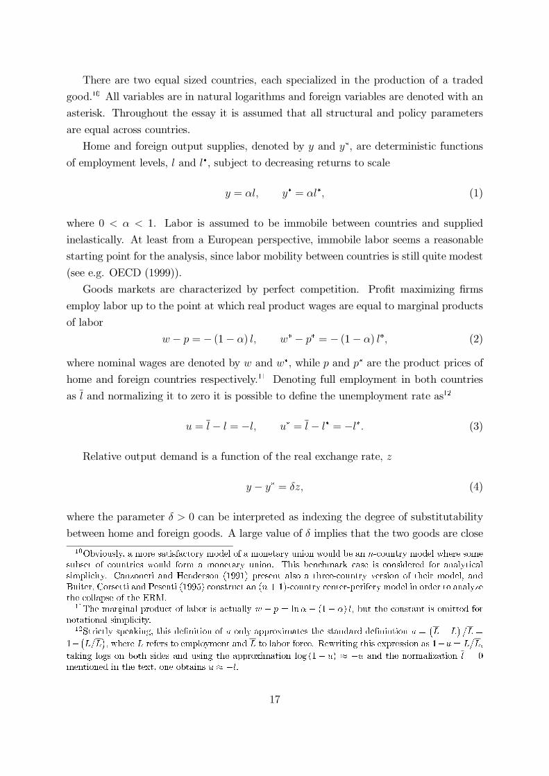
There are two equal sized countries, each specialized in the production of a traded

good.10 All variables are in natural logarithms and foreign variables are denoted with an

asterisk. Throughout the essay it is assumed that all structural and policy parameters

are equal across countries.

Home and foreign output supplies, denoted by y and y∗, are deterministic functions

of employment levels, l and l∗, subject to decreasing returns to scale

y = αl, y∗ = αl∗, (1)

where 0 < α < 1. Labor is assumed to be immobile between countries and supplied

inelastically. At least from a European perspective, immobile labor seems a reasonable

starting point for the analysis, since labor mobility between countries is still quite modest

(see e.g. OECD (1999)).

Goods markets are characterized by perfect competition. Profit maximizing firms

employ labor up to the point at which real product wages are equal to marginal products

of labor

w − p = − (1− α) l, w∗ − p∗ = − (1− α) l∗, (2)

where nominal wages are denoted by w and w∗, while p and p∗ are the product prices of

home and foreign countries respectively.11 Denoting full employment in both countries

as l and normalizing it to zero it is possible to define the unemployment rate as12

u = l − l = −l, u∗ = l − l∗ = −l∗. (3)

Relative output demand is a function of the real exchange rate, z

y − y∗ = δz, (4)

where the parameter δ > 0 can be interpreted as indexing the degree of substitutability

between home and foreign goods. A large value of δ implies that the two goods are close

10Obviously, a more satisfactory model of a monetary union would be an n-country model where somesubset of countries would form a monetary union. This benchmark case is considered for analyticalsimplicity. Canzoneri and Henderson (1991) present also a three-country version of their model, andBuiter, Corsetti and Pesenti (1995) construct an (n+ 1)-country center-perifery model in order to analyzethe collapse of the ERM.

11The marginal product of labor is actually w − p = lnα − (1− α) l, but the constant is omitted fornotational simplicity.

12Strictly speaking, this definition of u only approximates the standard definintion u =(L− L

)/L =

1−(L/L

), where L refers to employment and L to labor force. Rewriting this expression as 1−u = L/L,

taking logs on both sides and using the approximation log (1− u) ≈ −u and the normalization l = 0mentioned in the text, one obtains u ≈ −l.

17

substitutes, and therefore a small change in the real exchange rate brings about a large

change in relative demand.

The real exchange rate is defined as the relative price of the foreign good in terms of

the domestic good, expressed in home country currency

z = e+ p∗ − p, (5)

where the nominal exchange rate, denoted by e, is the domestic price of foreign currency.

Hence, a decrease in z implies that domestic currency appreciates in real terms. By

definition, in a monetary union (the log of) the nominal exchange rate is zero, and the

real exchange rate is simply

z = p∗ − p. (6)

Assuming that the underlying preferences over consumption are Cobb-Douglas with

a constant share of imports, β, the domestic and foreign consumer price indices (CPIs)

are given by

π = (1− β) p+ β (e + p∗) = p+ βz, (7)

π∗ = β (p− e) + (1− β) p∗ = p∗ − βz. (8)

The value of β is restricted to lie in the interval 0 < β < 12, which is equivalent to

assuming a home bias in consumption.13 It seems that this is a rather mild restriction, as

there is a large empirical literature on the home bias in trade showing that people indeed

have a strong preference for consumption of their home country goods.14

Under flexible exchange rates money demand is assumed to be proportional to nominal

income and only domestic residents hold domestic money. The money markets are in

equilibrium when nominal money supplies, m and m∗, satisfy simple quantity equations

m = p+ y, m∗ = p∗ + y∗. (9)

In a monetary union there is only one currency, which is held by the residents of both

countries. Monetary equilibrium requires that union-wide money demand equals union-

wide money supply. Following Lane (1996), money demand is proportional to average

13This is a common assumption in the open-economy macro literature, see. e.g. Buiter, Corsetti andPesenti (1995), Lane (1996, 2000) and Zervoyianni (1997).

14See e.g. Obstfeld and Rogoff (2000) and references therein.

18

nominal income of the member countries

mu =1

2(p+ y) +

1

2(p∗ + y∗) , (10)

where mu is the union-wide money supply. It is assumed that the common money supply

is spread out equally on both member countries, and thus the common central bank can’t

affect the distribution of money supply across countries.

2.2 Labor Union and Central Bank Preferences

In each country there is a single monopoly union, which sets the nominal wage rate strate-

gically, that is, the union takes into account the following reactions from the monetary

authorities. Unions’ utility functions are given by

U = γ (w − π)− 1

2u2, U∗ = γ (w∗ − π∗)− 1

2u∗2, (11)

where w − π and w∗ − π∗ are the real consumer wages, and u and u∗ are unemployment

rates in the two countries. The unions’ utility depends positively on the real consumer

wage and negatively on unemployment, which is consistent with traditional labor union

theory (see e.g. Oswald (1985)).15 This is where the essay departs from much of the

recent literature on strategic interaction between labor unions and the central bank. In

most studies it is assumed that labor unions care not only about the real wage and

unemployment, but also about inflation per se.16

Why should labor unions be interested in inflation? The standard explanation is

that union members have some non-indexed nominal assets or incomes other than their

salaries, such as bank deposits or pensions, values of which are eroded by inflation.

However, pensioners are usually not labor union members, and it seems unlikely that

unions would look after their interests. In many contributions labor unions’ inflation

aversion is actually driving the results, and therefore a closer look on possible reasons for

15The linear-quadratic functional form is widely used in this literature (see e.g. Jensen (1993, 1997),Cukierman and Lippi (1999, 2001), Coricelli, Cukierman and Dalmazzo (2000, 2001) and Berger, deHaan and Eijffinger (2001)). As the utility is linear in the consumer real wage, parallel shifts in labordemand curve do not affect unemployment. Hence, the impact of monetary regime on the equilibriumrate of unemployment comes solely from changes in the slope of the labor demand curve. In other words,the establishment of a monetary union will affect equilibrium unemployment only if the real consumerwage elasticity of the labor demand is affected.

16See Cukierman and Lippi (1999) and references therein. However, Soskice and Iversen (2000),Coricelli, Cukierman and Dalmazzo (2000) and Lawler (2002) also abstract from labor union inflationaversion in a closed-economy setting. Holden (2003a) studies a small open-economy case and Coricelli,Cukierman and Dalmazzo (2001) build a two-country monetary union model.

19

inflation aversion would be desirable.17

Monetary policy is discretionary in the model and the loss functions describing policy

preferences are of standard quadratic type

L = π2 + λ(u− uf

)2, L∗ = π∗2 + λ

(u∗ − uf

)2, (12)

where 0 ≤ λ < ∞. Since the model is assumed to be completely symmetric, the policy

parameters describing the conservatism of the central bank, λ, and the unemployment

target, uf , are equal across countries.18 CPI inflation is defined as the difference between

the log price levels in current and previous periods, π − π−1. Without loss of generality,

π−1 is normalized to zero, and thus CPI and CPI inflation are equivalent in this setup.

The inflation target of the central banks is set to zero for analytic convenience.

The parameter λ reflects the relative weight placed by the central bank on unem-

ployment deviations from the target level. λ−1 thus measures the Rogoff (1985a) type

of conservatism of the central bank.19 The smaller λ is, the more the central bank cares

about inflation deviations and the less about unemployment, i.e. it allows unemployment

to deviate more from the target level in order to push inflation closer to zero. Nominal

money supplies, m and m∗, are the policy instruments of the central banks.20

In a monetary union the common central bank is assumed to care only about the

average rates of unemployment and inflation in the area

Lu =

(π + π∗

2

)2

+ λ

(u+ u∗

2− uu

)2

, (13)

where uu is the unemployment target of the common central bank.21 It is assumed that

conservatism of the central bank, λ, will be unchanged when the monetary union is

established.

The aim of the essay is to demonstrate that the formation of a monetary union will

17A step into this direction is taken in Berger, Hefeker and Schöb (2002), where inflation aversion isendogenized by assuming that the outside option of the labor union is defined in nominal terms.

18The superscript f refers to a flexible exchange rate regime.19It would be conceptually clearer to write the weight parameter in front of the inflation term in the

loss function. Then the parameter would have a direct interpretation as the degree of conservatism. Thechoice made in this essay, however, makes some derivations simpler.

20This assumption is, admittedly, at odds with reality, since monetary policy is usually conductedwith the short-term nominal interest rate as the instrument. Money supply is, however, a natural choicehere as the model is static. Using interest rates as instruments in a static model would be conceptuallyconfusing, as interest rates are intertemporal by definition.

21Gros and Hefeker (2002) investigate how the common central bank’s choice of policy targets, that is,average monetary union wide welfare losses vs. the sum of national welfare losses, will affect the welfarein member countries in a heterogeneous monetary union.

20

have real effects independent of the existence of an inflation bias. Therefore, the central

bank’s unemployment target both under flexible exchange rates and in a monetary union

are assumed to be set at an arbitrary level, and it will be shown that the real economy is

unaffected by the chosen level. In particular, even though the target would coincide with

the equilibrium rate, the real effects will remain.

2.3 Timing of the Model

Events unfold as follows. (i) The two labor unions set their nominal wages simultaneously

taking the other union’s wage as given. They have full information about the reaction

functions of the central banks and take them into account in the wage setting process.

In other words, unions act strategically as Stackelberg leaders against the central banks.

(ii) Under flexible exchange rates the central banks choose their money supplies simulta-

neously taking the other central bank’s money supply as well as previously set nominal

wages as given. In a monetary union the common central bank sets the union-wide money

supply. (iii) Production and trade take place and macroeconomic outcomes are realized.

The choice of modelling the game between labor unions and central banks as a Stack-

elberg game is supported by observations in the real world wage setting and monetary

policy practices. Wage contracts are usually negotiated to cover at least a year, whereas

monetary policy can be adjusted frequently. It is assumed that the central banks don’t

have access to a commitment technology. In other words, the essay considers time-

consistent discretionary monetary policy. If the central banks could credibly commit to

a certain policy rule in advance, it might still be the case that monetary union would

affect equilibrium unemployment. All what is needed to generate changes in equilibrium

unemployment is that from a labor union’s perspective the optimal rule for the com-

mon central bank is different from the optimal rules of the national central banks. This

conjecture is, however, not investigated further in this essay.

The behavior of the labor unions can be time-inconsistent as well. It may be the

case that after the central banks have set their policies, the labor unions find it optimal

to renege on the wage contracts and set new, higher or lower, nominal wages. This

possibility is ruled out by assuming that nominal wage contracts are legally binding for

the whole contract period.

21

3 Monetary Policy and Wage Setting

In this section the two-stage game between labor unions and central banks is solved

in both monetary regimes by backward induction.22 Starting from the second stage,

equilibrium strategies are presented for central banks in a flexible exchange rate regime,

and for a common central bank in a monetary union case. Then the wage setting problem

at the first stage is solved and equilibrium outcomes are derived for macroeconomic

variables.

3.1 Monetary Policy in a Flexible Exchange Rate Regime

The reduced forms for home and foreign rates of unemployment and inflation in a flexible

exchange rate regime can be derived from equations (1)-(5) and (7)-(9)23

u = −m+ w, u∗ = −m∗ + w∗, (14)

π = (1− α)m+ αw +αβ

δ(m− w −m∗ + w∗) , (15)

π∗ = (1− α)m∗ + αw∗ − αβ

δ(m− w −m∗ + w∗) . (16)

Equation (14) shows that a domestic wage increase has a direct effect on unemployment

in home country, whereas foreign unemployment is unaffected. The home product price

is increased (see equation (47) in the Appendix) in order to balance the money market.

The real exchange rate appreciates so that the goods markets are in equilibrium (see

equation (48) in the Appendix). This reduces domestic consumer prices and increases

foreign consumer prices. The total effect on domestic CPI is ambiguous, but the foreign

CPI increases, i.e. inflation is exported by a unilateral wage increase.

Next, consider a unilateral domestic monetary expansion. Domestic unemployment

falls, and to balance the money market the product price increases (see equation (47)

in the Appendix). Goods market equilibrium calls for real exchange rate depreciation.

Domestic CPI increases and foreign CPI decreases because of the real exchange rate

depreciation.

The home country central bank’s problem is to minimize the loss function L in (12)

with respect tom, and subject to (14) and (15), taking nominal wages and foreign money

22The third stage of the game involves no strategic choices, since product markets are assumed to becompetitive.

23The reduced forms for the other endogenous variables are presented in the Appendix as equations(47)-(49).

22

supply m∗ as given. The first-order condition becomes

π =λ

1− α + αβ

δ

(u− uf

), (17)

which reveals that whenever the unemployment target is below the equilibrium rate of

unemployment, an inflation bias emerges.

Inserting the reduced forms (14) and (15) into the first-order condition and solving it

explicitly for m, yields the reaction function of the home central bank

m =λ− Γ

(α− αβ

δ

)(λ+ Γ2)

w +Γαβ

δ

(λ+ Γ2)(m∗ − w∗)− λ

(λ+ Γ2)uf , (18)

where Γ = 1 − α + αβδ−1. Depending on central bank conservatism, λ−1, the central

bank reacts to a domestic wage increase either by expanding or contracting money supply.

Cukierman, Rodrigues and Webb (1998) provide empirical evidence on monetary policy

responses to wage increases. Their results show that in countries with highly conservative

central banks, monetary policy is tightened in response to high wage settlements, whereas

in countries with less conservative central banks monetary policy is accommodating.

Due to perfect symmetry of the model, the foreign money supply schedule can be

written symmetrically. The two central banks choose their non-cooperative policies si-

multaneously. The Nash equilibrium policy for the home country is given by24

m = cf1w + cf2w∗ + cf3u

f , cf1 0, cf2 ≤ 0,−1 < cf3 ≤ 0, (19)

where the superscript f refers to the flexible exchange rate regime. The interpretation of

cf1 , cf2 and cf3 is straightforward. Home country wage increase induces either negative or

positive monetary policy reaction in equilibrium depending on central bank conservatism.

Since wage increase in the foreign country doesn’t directly affect home country unem-

ployment and is always inflationary, home country money supply is always reduced in

equilibrium. Also, it is intuitive that, other things equal, an increase in the unemployment

target calls for a reduction in money supply in equilibrium.

Finally, inserting equation (19) into equations (14) and (15) yields the rates of unem-

24The explicit forms of cf1 , cf2 and cf3 are given in the Appendix. An analogous equation holds for the

foreign country and is given by m∗ = cf1w∗ + cf2w + cf3u

f .

23

ployment and inflation as functions of home and foreign nominal wages25

u = af1w + af2w∗ + af3u

f , af1 > 0, af2 ≥ 0, 0 ≤ af3 < 1, (20)

π = bf1w + bf2w∗ + bf3u

f , bf1 ≥ 0, bf2 ≥ 0,−1 < bf3 ≤ 0, (21)

where, as before, the superscript f refers to the flexible exchange rate regime. These two

equations contain the optimal monetary policy responses to unions’ nominal wage claims.

At the first stage of the game, labor unions rationally anticipate the policy responses and

take them into account in wage setting, that is, the labor unions set wages strategically.

The nominal wage elasticity of unemployment, af1 , is always positive. The central

bank will accommodate the wage increase only partially, since money supply increases

are inflationary. If the central bank is conservative enough, it will contract money supply

in response to a wage increase, which implies that af1 can be greater than unity. Domestic

nominal wage increase will thereby always increase domestic unemployment. Less obvious

is the fact that a unilateral foreign nominal wage hike will increase unemployment in

home country, that is, af2 ≥ 0. However, the explanation is simple and can be seen

from the reduced forms in equations (14)-(16). The direct effect of foreign wages on

domestic unemployment is nil (see equation (14)), and the direct effect on domestic

inflation is positive (see equation (15)). Therefore, as long as the domestic central bank

targets both inflation and unemployment deviations, it will reduce money supply in order

to push inflation down. Since the domestic nominal wage is assumed to be unaltered,

unemployment will go up (see equation (14)). Other things equal, an increase in uf will

induce higher unemployment, since monetary policy will be more contractionary.

The nominal wage elasticities of inflation, bf1 and bf2 , are both positive, i.e. wage

increases are always inflationary. Only in the special case of ultra-conservative central

banks with λ = 0, will bf1 and bf2 be zero. As noted above, an increase in uf raises u.

But, due to af3 < 1, u − uf gets smaller and from (17) it follows that the inflation bias

problem will be reduced.

3.2 Monetary Policy in a Monetary Union

As in the previous section, first the reduced forms for rates of unemployment and inflation

are solved from equations (1)-(4), (6)-(8) and (10). By definition, (the log of) the nominal

exchange rate now equals zero, and the real exchange rate is simply expressed as the

difference of (the logs of) the foreign and domestic product prices in equation (6). Money

demand depends on the average union-wide nominal income. The reduced forms are

25The explicit forms of the elasticities are given in the Appendix.

24

given by26

u = −mu +1

2(w + w∗) +

1

2

δ

α + (1− α) δ(w − w∗) , (22)

u∗ = −mu +1

2(w + w∗)− 1

2

δ

α + (1− α) δ(w − w∗) , (23)

π = (1− α)mu + w −(1− α

2

)(w + w∗) (24)

−1

2

(2αβ + (1− α) δ

α + (1− α) δ

)(w − w∗) ,

π∗ = (1− α)mu + w∗ −(1− α

2

)(w + w∗) (25)

+1

2

(2αβ + (1− α) δ

α + (1− α) δ

)(w − w∗) .

From (22) one sees that in a monetary union unemployment depends directly on both

domestic and foreign wages, whereas in a flexible exchange rate regime only domestic

wage entered the unemployment equation.27 This interdependence in a monetary union

results from money market equilibrium (10), which can be rewritten as

mu =1

2(p+ y) +

1

2(p∗ + y∗) =

1

2(w − u) +

1

2(w∗ − u∗) . (26)

In a flexible exchange rate regime a unilateral wage increase doesn’t directly affect real

variables in the other country, while in a monetary union unemployment (and output)

in both countries will in general be affected. From (26) one sees that an increase of w

generally affects both u and u∗ when mu and w∗ are fixed.28

As expected, the reduced forms (22)-(25) reveal that an increase in the area-wide

money supply, mu, affects both countries symmetrically. Hence, the common central

bank can’t affect the real exchange rate, z, which is solely determined by the labor

unions (see equation (52) in the Appendix).

The common central bank chooses mu in order to minimize the loss function (13)

subject to (22)-(25). The first-order condition of the common central bank’s optimization

26The reduced forms for the other endogenous variables are presented in the Appendix as equations(50)-(52).

27Unemployment depends indirectly on both home and foreign wages in a flexible exchange rate regime,because monetary policies in both countries are affected by both w and w∗.

28From (22) one sees, however, that when δ = 1, unemployment depends directly only on the homecountry wage.

25

problem can be written as

π + π∗

2=

λ

(1− α)

(u+ u∗

2− uu

), (27)

which relates the average rate of inflation to the average rate of unemployment in the

monetary union area. Comparing this expression with equation (17), one finds that with a

given difference between the average rate of unemployment and the unemployment target,

average inflation is higher in a monetary union than under flexible exchange rates. As

mentioned in Introduction, a similar result is obtained in monetary policy cooperation

case (see e.g. Rogoff (1985b)).

Solving the first-order condition explicitly for mu yields the reaction function of the

common central bank

mu =λ− α (1− α)

2(λ+ (1− α)2

) (w + w∗)− λ(λ+ (1− α)2

)uu. (28)

The central bank’s reaction to wage increases is symmetric in a sense that the monetary

policy reaction to a unilateral wage increase doesn’t depend on which country is the

source. This characteristic obviously results from the assumed symmetry of the model.

If the central bank is conservative enough, it reduces money supply when nominal wages

are raised.

Finally, the rates of unemployment and inflation as functions of the nominal wages in

both countries and unemployment targets are derived by inserting the reaction function

(28) into the reduced forms of u and π29

u = au1w + au2w∗ + au3u

u, au1 > 0, au2 0, 0 ≤ au3 < 1, (29)

π = bu1w + bu2w∗ + bu3u

u, bu1 > 0, bu2 0,−1 < bu3 ≤ 0, (30)

where the superscript u refers to the monetary union case. Earlier it was shown that af2

is always positive. Now, au2 can be negative, i.e. a foreign wage increase may lower un-

employment in home country. This may happen if the common central bank is relatively

“liberal” (λ is large), or if the goods are close substitutes (δ is large). The difference

comes from the fact that the response of the common central bank to a unilateral wage

increase by one labor union is symmetric in both countries. It is instructive to consider

a case of a relatively liberal central bank, i.e. λ is large. Now, by setting δ = 1 the direct

effect of a foreign wage increase on domestic unemployment is nil as in a flexible exchange

29The explicit forms for the elasticities are given in the Appendix.

26

rate regime (see footnote 28 and equations (14) and (22)). The average area-wide unem-

ployment will increase, since foreign unemployment goes up and home unemployment is

unaffected. Now, given that the common central bank is fairly liberal, it will increase the

area-wide money supply so as to pull down the average unemployment rate. Since the

direct effect of a foreign wage increase on domestic unemployment is nil, accommodating

monetary policy will lower the domestic rate of unemployment below the initial level and

the total effect is thus negative.

The home country nominal wage elasticity of inflation, bu1 , is always positive in a

monetary union. However, the foreign country nominal wage elasticity of inflation, bu2 , can

be negative, if the common central bank is very conservative, i.e. λ is very small. Again,

this is caused by the inability of the common central bank to respond asymmetrically

to a unilateral wage increase. An increase in foreign wage level increases home inflation

less than foreign inflation, provided that β < 12(as assumed in the model). If the central

bank is very conservative, it will push the average inflation close to zero by reducing the

common money supply. Thereby, the home country inflation can become negative. It is

noteworthy that in this model the inflation rates of the member countries of a monetary

union need not to be equal, as it is the case e.g. in Grüner and Hefeker (1999) and

Cukierman and Lippi (2001).30

3.3 Strategic Wage Setting and Equilibrium Unemployment

The labor unions choose their wages in the first stage of the game taking the other union’s

wage as given. The unions have complete information about the reaction functions of the

central banks and they realize that since they are large enough, their wage claims will

affect the monetary policy. Hence, the unions set their wages strategically taking into

account the following monetary policy responses.

The labor unions maximize their utility functions (11) subject to (20) and (21) in a

flexible exchange rate regime, and subject to (29) and (30) in a monetary union. Since

the form of the wage setting problem is similar in both monetary regimes, the regime

in question is denoted with a superscript i whenever making a distinction between the

variables of the two regimes is not necessary. Solving the first-order condition for wi

yields a reaction function of the form

wi = γ(1− bi1)

(ai1)2 − ai2

ai1(w∗)i − ai3

ai1ui, (31)

30Even though the model allows inflation differences between the member countries in a monetaryunion, the equilibrium rate of inflation will be equal since the model is symmetric.

27

where i = f, u. Again, the symmetry of the model implies that the reaction function of

the foreign union is of the same form. In Nash equilibrium nominal wages are given by

wi = (w∗)i = γ(1− bi1)

ai1 (ai1 + ai2)

− ai3(ai1 + ai2)

ui. (32)

Inserting the equilibrium nominal wage (32) into the reduced form of the rate of

unemployment, (20) or (29), yields equilibrium unemployment

ui = (u∗)i = γ(1− bi1)

ai1. (33)

It is noteworthy that equilibrium unemployment is independent of the central banks’

unemployment target ui.

Once equilibrium unemployment levels in both countries are derived, equilibrium in-

flation rates can be obtained from equations (17) and (27). Rantala (2001) analyzes

the case where ui = 0. However, for the purpose of this essay it suffices to notice that

equilibrium unemployment doesn’t depend on ui. It follows that even though the un-

employment target ui would coincide with the equilibrium rate of unemployment, which

results in the disappearance of inflation bias (see equations (17) and (27)), the real effects

brought about by the establishment of a monetary union, which are discussed in the next

section, remain unchanged. Moreover, equation (33) reveals the source of unemployment

in the model. The equilibrium rate of unemployment is always positive, provided that

the labor unions have a real wage target, i.e. γ > 0.

In order to gain some intuition on the unemployment determination in the model, it

is instructive to study the labor union’s wage setting in unemployment—real wage space.

Employment, and thus also unemployment, is determined from the labor demand curve.

From equations (2) and (3) one observes that the slope of the labor demand curve in

(ui, (wi − pi)) space is (1− α).31 However, the labor union’s utility depends on the real

consumer wage and the rate of unemployment. Contrary to the real product wage, wi−pi,

the real consumer wage, wi − πi, contains also foreign product price as an element, and

it turns out to be useful to study the effective labor demand curve for the union in

31Since the variables are in logs, the slope coefficient can be directly converted into real product wageelasticity of labor demand, η ≡ − ∂ logN

∂ logW/P = − ∂l∂(w−p) = ∂u

∂(w−p) = 11−α ∈ (1,∞), which in this model

depends only on production technology.

28

(ui, (wi − πi)) space32

(wi − πi

)=

1− bi1ai1

ui − ai1bi2 + (1− bi1) a

i2

ai1(w∗)i (34)

−ai1bi3 + (1− bi1) a

i3

ai1ui.

The slope coefficient, (1− bi1) /ai1, of the effective labor demand curve (34) together with

the labor union preference parameter, γ, directly determine the equilibrium rate of un-

employment in the model (see equation (33)). Figure 1, where one indifference curve of

the labor union is denoted by U((w − π) , u; γ), illustrates the equilibrium.

u

w-π U((w-π),u;γ)

slope (1-b1)/a1

Figure 1: Determination of equilibrium unemployment

The slope coefficient (1− bi1) /ai1 can be written as a function of the two nominal wage

elasticities of unemployment, ai1 and ai233

1− bi1ai1

= (1− α) +αβ

δ

(ai1 − ai2

ai1

). (35)

This formulation is helpful in unemployment comparisons between the two monetary

regimes presented in the next section. Equilibrium unemployment depends on two elas-

ticities. The first one is the nominal wage elasticity of the real exchange rate, which is

given by ∂z/∂wi = −αδ−1 (ai1 − ai2) ≤ 0. The stronger effect the wage has on the real

exchange rate, the steeper is the effective labor demand curve. The second elasticity is

32This expression is obtained from equations (20) and (21) (or from (29) and (30)).33Derivation of this expression can be found in the Appendix.

29

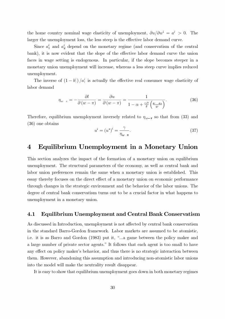
the home country nominal wage elasticity of unemployment, ∂u/∂wi = ai1 > 0. The

larger the unemployment loss, the less steep is the effective labor demand curve.

Since ai1 and ai2 depend on the monetary regime (and conservatism of the central

bank), it is now evident that the slope of the effective labor demand curve the union

faces in wage setting is endogenous. In particular, if the slope becomes steeper in a

monetary union unemployment will increase, whereas a less steep curve implies reduced

unemployment.

The inverse of (1− bi1) /ai1 is actually the effective real consumer wage elasticity of

labor demand

ηw−π = − ∂l

∂ (w − π)=

∂u

∂ (w − π)=

1

1− α + αβ

δ

(a1−a2a1

) . (36)

Therefore, equilibrium unemployment inversely related to ηw−π so that from (33) and

(36) one obtains

ui = (u∗)i =γ

ηw−π. (37)

4 Equilibrium Unemployment in a Monetary Union

This section analyzes the impact of the formation of a monetary union on equilibrium

unemployment. The structural parameters of the economy, as well as central bank and

labor union preferences remain the same when a monetary union is established. This

essay thereby focuses on the direct effect of a monetary union on economic performance

through changes in the strategic environment and the behavior of the labor unions. The

degree of central bank conservatism turns out to be a crucial factor in what happens to

unemployment in a monetary union.

4.1 EquilibriumUnemployment and Central Bank Conservatism

As discussed in Introduction, unemployment is not affected by central bank conservatism

in the standard Barro-Gordon framework. Labor markets are assumed to be atomistic,

i.e. it is as Barro and Gordon (1983) put it, “...a game between the policy maker and

a large number of private sector agents.” It follows that each agent is too small to have

any effect on policy maker’s behavior, and thus there is no strategic interaction between

them. However, abandoning this assumption and introducing non-atomistic labor unions

into the model will make the neutrality result disappear.

It is easy to show that equilibrium unemployment goes down in both monetary regimes

30

when central bank conservatism increases (see the Appendix for derivations).34 The intu-

ition behind this somewhat surprising result is clear. When λ is small, i.e. conservatism

is high, labor unions correctly anticipate tight monetary policy and a large rise in un-

employment in response to their wage claims. Conservatism works as a deterrent to

wage increases and therefore moderates the labor unions’ real wage targets leading to

lower unemployment. This can be seen by differentiating the nominal wage elasticities of

unemployment with respect to λ in both regimes, which gives

∂af1∂λ

< 0,∂au1∂λ

< 0, (38)

where an increase in conservatism means that λ becomes smaller.

Strictly speaking, this argument is correct only in the monetary union case, where

the nominal wage elasticity of the real exchange rate doesn’t depend on central bank

conservatism. Under a flexible exchange rate an increase in conservatism strengthens

the union’s ability to appreciate the real exchange rate, which works into the opposite

direction and tends to increase wage demands. Differentiating (ai1 − ai2) (where i = f, u)

with respect to λ yields

∂(af1 − af2

)∂λ

< 0,∂ (au1 − au2)

∂λ= 0. (39)

As shown in the Appendix, the deterrent effect of central bank conservatism dominates

the real exchange rate effect, and therefore increased conservatism will decrease unem-

ployment also in a flexible exchange rate regime. Hall and Franzese (1998) and Cukierman

and Lippi (1999) provide some empirical evidence supporting the result. They show that

when bargaining structure is highly centralized, an increase in central bank conservatism

tends to lower unemployment.

34The flexible exchange rate case is presented in Jensen (2000), a fact which was kindly brought tothe author’s notice by Henrik Jensen after the working paper version of this essay (Rantala (2001)) waspublished.

31

4.2 The Impact of Monetary Union on Equilibrium Unemploy-

ment

The impact of the formation of a monetary union on equilibrium unemployment can be

analyzed by studying the following expression

sgn(uu − uf

)= −sgn

(au2au1

− af2

af1

), (40)

where the right-hand side is obtained from (35). In the Appendix it is proved that

there exists a unique non-negative cut-off point for central bank conservatism, λ, where

uu = uf . This critical value, λ, is given by

λ =1

2δ2

(−A+

√A2 +B

), (41)

A = (1− α)2 δ2 + α (1− α) (3β − 1) δ + 2α2β2,

B = 4δ2α (1− α)2 (1− 2β) (αβ + δ (1− α)) > 0,

where B > 0 holds, since β < 12. The equilibrium unemployment is lower in a monetary

union than under flexible exchange rate regime when central bank conservatism is high

enough, i.e. λ ∈ [0, λ). However, when λ ∈ (λ,∞) unemployment will be higher in a

monetary union. Figure 2 illustrates the result.

u

w-π U((w-π),u;γ)

uu uf uu

conservatism low

conservatism high

Figure 2: The impact of monetary union on equilibrium unemployment

This result is in sharp contrast with earlier results concerning the impact of mon-

etary union on equilibrium unemployment. Grüner and Hefeker (1999) show that the

32

establishment of a monetary union will increase unemployment, if national labor unions

are inflation averse. However, their result depends crucially on the assumed inflation

aversion, and thereby also on the existence of an inflation bias. The above result (41)

points out that in this model with open-economy spillovers, monetary union will have

real effects even when labor unions are not inflation averse, and without an inflation bias.

Interestingly enough, (41) indicates that one can always find a level of conservatism such

that monetary union will be beneficial in terms of reduced unemployment.

An intuitive explanation for the above result can be obtained by inspecting the labor

union’s incentives for wage hikes in the two alternative regimes with different degrees of

central bank conservatism. In a monetary union the real exchange rate is solely deter-

mined by nominal wages set by the labor unions. The conservatism of the central bank

will thereby not affect the unions’ ability to appreciate the real exchange rate. As noted

in the previous section, an increase in conservatism will improve the labor union’s ability

to appreciate the real exchange rate in the flexible exchange rate regime (see equation

(39)). When conservatism is fairly high, the central banks will give priority to inflation

deviations from the target. In the face of a unilateral wage increase, the central bank

of the country in question will tighten monetary policy considerably in order to bring

inflation down. In the other country the central bank will also tighten its policy, since

real exchange rate depreciation is inflationary, but to a lesser extent. The need to react

less vigorously results from the assumption of a home bias in consumption, which implies

that inflation reaction to a wage hike is stronger in the country in question.35 Hence, the

equilibrium response of the two central banks appreciates the real exchange rate further,

and thereby induces more aggressive wage policy than in the monetary union case, which

in turn leads to higher unemployment.

On the other hand, when central bank conservatism is low, that is, the focus is on

unemployment deviations from the target, the flexible exchange rate regime provides

weaker incentives to wage increases than a monetary union. Even though a labor union

tried to appreciate the real exchange rate with its wage claim, under a flexible exchange

rate the central banks will guarantee with their policies that unemployment rates remain

close to the target, which implies that ai1 and ai2 are close to zero. Keeping in mind that

∂z/∂wi = −αδ−1 (ai1 − ai2) ≤ 0, it becomes evident that the real exchange motive for

wage hikes is weak when conservatism is low. Irrespective of the degree of conservatism,

35To be precise, in a flexible exchange rate regime a unilateral wage increase will increase inflation inhome country more than in foreign country provided that the real exchange rate appreciation is not toostrong relative to the import share. From (15) and (16) one obtains a condition δ > 2β, which limits thesubstitutability parameter. This restriction is satisfied e.g. when one assumes Cobb-Douglas preferencesfor consumption, δ = 1, since β < 1

2 in the model. In a monetary union β < 12 is alone a sufficient

condition for home inflation reaction to exceed foreign reaction (see (24) and (25)).

33

monetary policy in a monetary union is incapable of affecting the real exchange rate,

and so monetary policy reactions can’t neutralize the impact of a unilateral wage hike

on the real exchange rate. It follows that in a monetary union, the labor unions do have

the real exchange motive for pushing up wages also when conservatism is low, and hence

their wage policy will be more aggressive than under flexible exchange rates, resulting in

higher unemployment.

5 Restoring Neutrality: Two Alternatives

This essay emphasizes that under fairly general conditions the formation of a monetary

union will affect the equilibrium rate of unemployment. It was argued that there are ba-

sically two critical assumptions, which are needed in order to generate the non-neutrality

result presented in the previous section: non-atomistic wage setting and imperfect sub-

stitutability between the two goods produced. This section relaxes these two conditions

and verifies the emergence of neutrality.

So far, the goods produced in the two countries were assumed to be imperfect substi-

tutes in consumption. This is captured in the model by the substitutability parameter,

δ, which describes how the relative price of the goods will affect their relative demand.

If δ approaches infinity, the two goods become perfect substitutes in consumption. It is

easy to show that in this case the equilibrium rate of unemployment becomes (see the

Appendix for derivations)

uf|δ→∞ = uu|δ→∞ = γ (1− α) . (42)

The neutrality result emerges, because perfect substitutability implies that the real ex-

change rate becomes exogenous to labor unions. There is effectively only one good in the

model. It follows that the purchasing power parity (PPP) has to hold and the real ex-

change rate can’t deviate from zero (in logs), because otherwise the world demand would

shift to one country. Hence, the labor unions’ incentives to push up nominal wages in

order to appreciate the real exchange rate are destroyed. Moreover, comparing (42) with

(33) and (35) one immediately sees that unemployment is lower when δ → ∞. The same

neutrality result is obtained in Grüner and Hefeker (1999) and Cukierman and Lippi

(2001), when unions are not inflation averse.

The model can easily be modified to show that non-atomistic wage setting is also

crucial for the non-neutrality result of the essay. Assuming that there is a continuum of

labor union—firm pairs indexed by j and distributed uniformly between j = 0 and j = 1

in both countries implies, that all unions take the product price and the consumer price

34

index as given in wage setting. Modifying (2) and (3), labor demand of the representative

firm, j, is given by

wj − p = − (1− α) lj = (1− α) uj. (43)

A representative union’s problem is then

maxwj

(γ (wj − π)− 1

2u2j

), (44)

s.t. (43) and π given.

The first-order condition becomes

wj − p = γ (1− α)2 . (45)

Inserting the real wage (45) into (43) yields the rate of unemployment in union j

uj = γ (1− α) .

Aggregation over all labor union—firm pairs gives the corresponding equation for the

national rate of unemployment

u =

∫ 1

j=0

ujdj = γ (1− α) , (46)

which is clearly independent of the monetary regime. When labor markets are atomistic,

the equilibrium rate of unemployment depends only on labor union preferences, γ, and

the real product wage elasticity of labor demand (see equation (43) and Footnote 31).

As expected, the unemployment outcome is the same as in the infinite substitution case

above, that is, (46) coincides with (42).

6 Concluding Remarks

The purpose of the essay is to study the impact of the formation of a monetary union

on the equilibrium rate of unemployment. In particular, it is shown that in the pres-

ence of strategic interaction between the central bank and the labor unions, changes in

monetary regime will have real effects. Monetary regime will affect the labor union’s real

wage—unemployment tradeoff, i.e. the real consumer wage elasticity of labor demand is

endogenous in the model.

The main result of the essay is that the establishment of a monetary union lowers

35

unemployment, provided that the degree of central bank conservatism is sufficiently high,

whereas with low degrees of conservatism unemployment goes up. Interestingly enough,

the inflexibility of the common central bank of the monetary union in responding to a

country specific wage increase is good news in terms of unemployment if the central bank

is conservative, whereas it is bad news if the central bank is fairly liberal. This result

indicates that the choice of a monetary regime and the way monetary policy is conducted

can be important factors in determining labor market outcomes in countries with highly

centralized wage setting. Importantly, and unlike in the previous literature in this field,

the results of the essay don’t depend on the existence of an inflation bias.

The assumption of a single union in each country is obviously quite restrictive, but

it can be justified as the simplest way to model non-atomistic labor markets. Labor is

homogenous in the model. Therefore, it makes no sense to consider different levels of

centralization of wage bargaining, since unions in this setup can’t raise their wages above

the average wage rate of the economy.36 One could follow Lippi (2002) and introduce

the level of centralization of wage bargaining into the model by assuming that labor is

differentiated in general, and that all types of labor are needed in the production of the

single good. Then each union has pricing power and the effects of centralization could

be inspected. One likely consequence is that the rate of unemployment would decrease

with the number of unions, since each union’s ability to appreciate the real exchange rate

with its wage claim would be reduced. However, it is unclear how this would affect the

relative unemployment performance of a monetary union.

The model belongs to a class of “traditional” open-economy models, which basically

are linearized versions of the Mundell-Fleming model. International spillovers operate

through the real exchange rate channel. A monetary expansion by one country will have

a beggar-thy-neighbor effect, since the depreciation of the real exchange rate will shift

world demand toward that country. Moreover, inflation will increase in that country and

decrease in the other country. Thus the other country will also devalue its currency by

expansionary monetary policy and this leads to a situation known as “competitive deval-

uations”. In the traditional literature on international policy coordination this spillover

effect creates an incentive to coordinate national monetary policies. However, as men-

36There is a voluminous literature on the degree of centralization of wage bargaining and its effectson macroeconomic performance. Calmfors and Driffill (1988) present the well-known “hump-shape”hypothesis, which states that macroeconomic performance is better under a fully decentralized, and onthe other hand, under a totally centralized wage bargaining systems than under intermediate levels ofcentralization, such as industry level bargaining. Open-economy considerations related to the hump-shape hypothesis are studied in Driffill and van der Ploeg (1993), Danthine and Hunt (1994) and Rama(1994). Interactions between the degree centralization of wage bargaining and monetary policy areanalyzed e.g. in Cukierman and Lippi (1999), Lippi (2002) and Holden (2003b).

36

tioned in Introduction, domestic credibility problems may get worse under cooperation.37

The analysis in this traditional open-economy framework lacks explicit micro-founda-

tions and the welfare criterion, like the widely used quadratic social welfare function, is

ad hoc.38 Recent contributions in the rapidly growing field of “new open-economy macro-

economics” have questioned the beggar-thy-neighbor effect in international transmission

of shocks from a country to another. The novelty of the approach initiated by Obstfeld

and Rogoff (1995, 1996) is in the fully-fledged micro-foundations, which enable the use

of the utility of the representative consumer as a welfare criterion in policy evaluation.39

Corsetti and Pesenti (2001) and Tille (2001) show that instead of being a beggar-thy-

neighbor, an unanticipated monetary expansion can in terms of welfare actually be a

beggar-thyself policy. The intuition behind this result is simple. Although a monetary

surprise raises output and employment, the associated exchange rate depreciation wors-

ens the terms of trade, thereby reducing the purchasing power of consumers. Then it

is possible that consumers are unable to buy enough additional consumption to offset

the cost of their increased effort. The main result is that if the substitutability of goods

across countries is low, the adverse terms of trade effect dominates and monetary ex-

pansion is a beggar-thyself policy in terms of welfare. In that case countries have no

incentives to boost employment through monetary expansions. This new result brought

about by explicit microeconomic underpinnings qualifies the policy implications of the

traditional literature by showing that the exchange rate channel may not be as strong as

the traditional Mundell-Fleming analysis, which is also applied in this essay, suggests.

The model offers insights for the desirable policy choices in a monetary union. Obvi-

ously, one has to be extremely cautious in drawing strong policy implications based on

such a simple model. The single union assumption clearly limits the applicability of the

model in policy analysis to countries with relatively centralized wage setting. The model

seems to suggest that when a monetary union is established, it is possible to attain lower

rate of equilibrium unemployment by delegating monetary policy to a sufficiently conserv-

ative central bank. In Europe the creation of the EMU has increased the degree of central

bank conservatism in most member countries. Thus, based on the analysis, one could

speculate that the EMU may well have positive effects on equilibrium unemployment in

many member countries. However, it must be stressed, that the deterministic analysis

conducted in the essay abstracts completely from stabilization problems in a stochastic

37See Persson and Tabellini (2000, Ch. 18) for discussion and analysis on competitive devaluations,credibility problems and proper institutions for sustaining desirable policies.

38However, it is well-known that this widely used functional form can be obtained as a second-orderTaylor series approximation to the level of expected utility of the representative household in an opti-mizing model with nominal price rigidities (see e.g. Woodford (2001)).

39Lane (2001) surveys the “new open-economy macroeconomics” literature.

37

setup. Central bank conservatism is a free lunch in the model. The policy implications

will probably change, if one takes into account that delegating monetary policy to a cen-

tral bank which is more conservative than the society will distort stabilization policy. It

is quite likely that a tradeoff between low equilibrium unemployment and stabilization

properties of the economy emerges, and that one can derive an optimal degree of central

bank conservatism, where the weight on unemployment deviations is strictly positive. A

thorough investigation of this point is left for future research.

38

A Appendix

A.1 Derivation of Endogenous Variables and Nominal Wage

and Unemployment Target Elasticities

The reduced forms for the other endogenous variables in the flexible exchange rate regime

are

p = (1− α)m+ αw, p∗ = (1− α)m∗ + αw∗, (47)

z =α

δ(m− w −m∗ + w∗) , (48)

e =(αδ+ (1− α)

)(m−m∗) +

(α− α

δ

)(w − w∗) . (49)

The Nash equilibrium nominal wage and unemployment target elasticities of money

supply in the flexible exchange rate regime are

cf1 =(λ+ Γ2)

(λ+ Γ

(αβ

δ− α

))−(αβ

δΓ)2

∆ 0,

cf2 = −αβ

δ

Γ2

∆≤ 0,

cf3 = − λ

(λ+ Γ (1− α))u ≤ 0,

where Γ = 1− α + αβδ−1 and ∆ = (λ+ Γ2)2 −

(αβ

δΓ)2

> 0.

The nominal wage and unemployment target elasticities of unemployment and infla-

tion in the flexible exchange rate regime are

af1 =Γ (λ+ Γ2)

∆> 0,

af2 =αβ

δ

Γ2

∆> 0,

af3 =λ

(λ+ Γ (1− α))≥ 0,

bf1 =λ (λ+ Γ2)

∆≥ 0,

bf2 =αβ

δ

λΓ

∆≥ 0,

bf3 = − λ (1− α)

(λ+ Γ (1− α))≤ 0.

39

The reduced forms for the other endogenous variables in the monetary union case are

p = w + (1− α)mu − (1− α)

2(w + w∗) (50)

+1

2

(1− α) δ

α + (1− α) δ(w∗ − w) ,

p∗ = w∗ + (1− α)mu − (1− α)

2(w + w∗) (51)

−1

2

(1− α) δ

α + (1− α) δ(w∗ − w) ,

z =α

α + (1− α) δ(w∗ − w) . (52)

The nominal wage and unemployment target elasticities of unemployment and infla-

tion in the monetary union case are

au1 =

((1− α) (α + 2 (1− α) δ) + δλ

Ω

)> 0,

au2 =

(α (1− α)− δλ

Ω

) 0,

au3 =λ

λ+ (1− α)2≥ 0,

bu1 =

(λ+ (1− α)2

)(2α (1− β) + (1− α) δ)

Ω

− (1− α)2 (α + (1− α) δ)

Ω> 0,

bu2 =

(λ+ (1− α)2

)(2αβ + (1− α) δ)

Ω

− (1− α)2 (α + (1− α) δ)

Ω 0,

bu3 =−λ (1− α)(λ+ (1− α)2

) ≤ 0,

where Ω = 2(λ + (1− α)2

)(α + (1− α) δ) > 0.

40

A.2 Derivation of Equation (35)

Under a flexible exchange rate, from the reduced forms (14) and (15) one obtains

af1 = −∂mf

∂w+ 1,

1− bf1 = (1− α)

(1− ∂mf

∂w

)− αβ

δ

(∂mf

∂w− 1− ∂m∗f

∂w

),

and by noting, that ∂m∗

∂w= −af2 (see the Appendix A.1) the slope coefficient (35) can be

written as1− bf1

af1= (1− α) +

αβ

δ

(af1 − af2

af1

).

Similarly, in a monetary union case one obtains

au1 = −∂mu

∂w+

1

2+

δ

2 (α + (1− α) δ),

1− bu1 = (1− α)

(−∂mu

∂w+

1

2+

δ

2 (α + (1− α) δ)

)

+αβ

(α + (1− α) δ).

From equations (1), (3) and (4) one gets z = αδ(l − l∗) = −α

δ(u− u∗) and ∂z

∂w=

−αδ(a1 − a2). From (52) one obtains ∂z

∂w= − α

α+(1−α)δ, which implies that

α

α + (1− α) δ=

α

δ(au1 − au2) .

Inserting this expression into 1− bu1 above yields

1− bu1 = (1− α) au1 +αβ

δ(au1 − au2) .

Hence, the form of the slope coefficient is similar to the flexible exchange rate case

1− bu1au1

= (1− α) +αβ

δ

(au1 − au2

au1

).

41

A.3 Derivation of the Impact of Conservatism on Equilibrium

Unemployment

The rates of equilibrium unemployment in both regimes are given by equation (33). Then,

equation (35) implies, that sgn(∂u∂λ

)= −sgn

(∂(a2a1

)/∂λ

)in both regimes. FromAppen-

dix A.1 one obtainsaf2

af1

=(αβδ )Γλ+Γ2

andau2

au1

= α(1−α)−δλ(1−α)(α+2(1−α)δ)+δλ

. Differentiation of these ex-

pressions with respect to λ yields ∂(af2

af1

)/∂λ < 0 and ∂

(au2

au1

)/∂λ = −δ((1−α)(2α+2(1−α)δ))

((1−α)(α+2(1−α)δ)+δλ)2<

0. Hence ∂uf

∂λ> 0 and ∂uu

∂λ> 0.

A.4 Derivation of Equation (41)

Equation (35) implies, that sgn(uu − uf

)= −sgn

(au2

au1

− af2

af1

). The expression in brackets

on the right hand side can be written as

au2au1

− af2

af1=

α (1− α)− δλ

(1− α) (α + 2 (1− α) δ) + δλ−

αβ

δ

(1− α + αβ

δ

)λ+

(1− α + αβ

δ

)2= δ

(−δ2λ2 +

(δ(α (1− α)− δ (1− α)2

)− αβ (3δ (1− α) + 2αβ)

)λ)

(2δ (1− α)2 + α (1− α) + λδ

) (λδ2 + δ2 (1− α)2 + 2αβδ (1− α)

)+δ

α (1− α)2 (1− 2β) (δ (1− α) + αβ)(2δ (1− α)2 + α (1− α) + λδ

) (λδ2 + δ2 (1− α)2 + 2αβδ (1− α)

) .The denominator is always positive, and thus the quadratic function of λ in the numerator

determines the sign of the expression. Since the constant term in the numerator is

positive, and the coefficient in front of the quadratic term is negative, it follows that the

quadratic function has only one positive real root. Solving the quadratic equation

−δ2λ2 +(δ(α (1− α)− δ (1− α)2

)− αβ (3δ (1− α) + 2αβ)

)λ

+α (1− α)2 (1− 2β) (δ (1− α) + αβ) = 0

yields two real roots, of which only the bigger one is positive

λ =1

2δ2

(−A+

√A2 +B

),

A = (1− α)2 δ2 + α (1− α) (3β − 1) δ + 2α2β2,

B = 4δ2α (1− α)2 (1− 2β) (αβ + δ (1− α)) > 0.

42

Hence,(au2

au1

− af2

af1

)> 0 when λ ∈ [0, λ) and

(au2

au1

− af2

af1

)< 0 when λ ∈ (λ,∞). Since

sgn(uu − uf

)= −sgn

(au2

au1

− af2

af1

), it follows that uu < uf provided that λ ∈ [0, λ).

A.5 Derivation of Equation (42)

The nominal wage elasticities of unemployment in a flexible exchange rate regime with

infinite substitutability between goods, δ → ∞, can be written as af1|δ→∞ = (1−α)

λ+(1−α)2and

af2|δ→∞ = 0. Unemployment is then given by

uf|δ→∞ = γ

((1− α) +

αβ

δ

(1− af2

af1

))= γ (1− α) .

In a monetary union the nominal wage elasticities of unemployment are

au1|δ→∞ =

(2 (1− α)2 + λ

2((1− α)2 + λ

)(1− α)

),

au2|δ→∞ = − λ

2((1− α)2 + λ

)(1− α)

.

It follows thatau2

au1

= − λ

2(1−α)2+λ, and unemployment is given by

uu|δ→∞ = γ

((1− α) +

αβ

δ

(1− au2

au1

))= γ (1− α) .

43

References

[1] Barro, R. J. and D. B. Gordon (1983), “A Positive Theory of Monetary Policy in a

Natural Rate Model”, Journal of Political Economy 91, 589-610.

[2] Berger, H., J. de Haan and S. C. W. Eijffinger (2001), “Central Bank Independence:

An Update of Theory and Evidence”, Journal of Economic Surveys 15, 3-40.

[3] Berger, H., C. Hefeker and R. Schöb (2002), “Optimal Central Bank Conservatism

and Monopoly Trade Unions”, IMF Working Paper 02/44, International Monetary

Fund, Washington.

[4] Blinder, A. S. (1998), Central Banking in Theory and Practice, MIT Press, Cam-

bridge, MA.

[5] Buiter, W. H., C. Corsetti and P. A. Pesenti (1995), “A Center-Periphery Model

of Monetary Coordination and Exchange Rate Crises”, NBER Working Paper No.

5140.

[6] Burda, M. C. (1999), “European Labour Markets and the Euro: How Much Flexi-

bility Do We Really Need?”, CEPR Discussion Paper No. 2217.

[7] Calmfors, L. (2001a), “Unemployment, Labor Market Reform andMonetary Union”,

Journal of Labor Economics 19, 265-289.

[8] Calmfors, L. (2001b), “Wages and Wage-Bargaining Institutions in the EMU — A

Survey of the Issues”, Empirica 28, 325-351.

[9] Calmfors, L., A. Booth, M. Burda, D. Checchi, R. Naylor, J. Visser (2001), “The Fu-

ture of Collective Bargaining in Europe” in T. Boeri, A. Brugiavini and L. Calmfors,

Eds., The Role of Unions in the Twenty-First Century, Oxford University Press,

Oxford.

[10] Calmfors, L. and J. Driffill (1988), “Bargaining Structure, Corporatism and Macro-

economic Performance”, Economic Policy 6, 14-61.

[11] Canzoneri, M. B. and D. W. Henderson (1988), “Is Sovereign Policymaking Bad?”,

Carnegie-Rochester Conference Series on Public Policy 28, 93-140.

[12] Canzoneri, M. B. and D. W. Henderson (1991), Monetary Policy in Interdependent

Economies: A Game-Theoretic Approach, MIT Press, Cambridge, MA.

44

[13] Coricelli, F., A. Cukierman and A. Dalmazzo (2000), “Monetary Institutions, Mo-

nopolistic Competition, Unionized Labour Markets and Economic Performance”,

CEPR Discussion Paper No. 2407.

[14] Coricelli, F., A. Cukierman and A. Dalmazzo (2001), “Economic Performance and

Stabilization Policy in a Monetary Union with Imperfect Labor and Goods Mar-

kets”, forthcoming in H. W. Sinn, M. Widgren and M. Kothenburger, Eds., Issues

of Monetary Integration in Europe, MIT Press, Cambridge, MA.

[15] Corsetti G. and P. Pesenti (2001), “Welfare and Macroeconomic Interdependence”,

Quarterly Journal of Economics 116, 421-445.

[16] Cukierman, A., P. Rodrigues and S. B. Webb (1998), “Central Bank Autonomy

and Exchange Rate Regimes—Their Effects on Monetary Accommodation and Ac-

tivism” in S. Eijffinger and H. Huizinga, Eds., Positive Political Economy: Theory

and Evidence, Cambridge University Press, Cambridge.

[17] Cukierman, A. and F. Lippi (1999), “Central Bank Independence, Centralization

of Wage Bargaining, Inflation and Unemployment: Theory and Some Evidence”,

European Economic Review 43, 1395-1434.

[18] Cukierman, A. and F. Lippi (2001), “Labour Markets and Monetary Union: A

Strategic Analysis”, Economic Journal 111, 541-565.

[19] Danthine, J.-P. and J. Hunt (1994), “Wage Bargaining Structure, Employment and

Economic Integration”, Economic Journal 104, 528-541.

[20] Driffill, J. and F. van der Ploeg (1993), “Monopoly Unions and the Liberalisation of

International Trade”, Economic Journal 103, 379-385.

[21] Friedman, M. (1968), “The Role of Monetary Policy”, American Economic Review

58, 1-17.

[22] Gros, D. and C. Hefeker (2002), “One Size Must Fit All: National Divergences in a

Monetary Union”, German Economic Review 3, 247-262.

[23] Grüner, H. P. and C. Hefeker (1999), “How Will EMU Affect Inflation and Unem-

ployment in Europe?”, Scandinavian Journal of Economics 101, 33-47.

[24] Hall, P. A. and R. J. Franzese, Jr. (1998), “Mixed Signals: Central Bank Indepen-

dence, Coordinated Wage Bargaining, and European Monetary Union”, Interna-

tional Organization 52, 505-535.

45

[25] Holden, S. (2003a), “Wage Setting under Different Monetary Regimes”, Economica

70, 251-265.

[26] Holden, S. (2003b), “Monetary Regimes and the Co-ordination of Wage Setting",

forthcoming in European Economic Review.

[27] Jensen, H. (1993), “International Monetary Policy Cooperation in Economies with

Centralized Wage Setting”, Open Economies Review 4, 269-285.

[28] Jensen, H. (1997), “Monetary Policy Cooperation May Not Be Counterproductive”,

Scandinavian Journal of Economics 99, 73-80.

[29] Jensen, H. (2000), “Inflation Aversion and Equilibrium Activity in Jensen (1993)”,

mimeo, University of Copenhagen.

[30] Kydland, F. E. and E. C. Prescott (1977), “Rules Rather than Discretion: The

Inconsistency of Optimal Plans”, Journal of Political Economy 85, 473-491.

[31] Lane, P. R. (1996), “Stabilization Policy in a Currency Union”, Economics Letters

53, 53-60.

[32] Lane, P. R. (2000), “Asymmetric Shocks and Monetary Policy in a Currency Union”,

Scandinavian Journal of Economics 102, 585-604.

[33] Lane, P. R. (2001), “The New Open Economy Macroeconomics: A Survey”, Journal

of International Economics 54, 235-266.

[34] Lawler, P. (2002), “Monetary Uncertainty, Strategic Wage Setting and Equilibrium

Employment”, Economics Letters 77, 35-40.

[35] Lippi, F. (2002), “Strategic Monetary Policy with Non-Atomistic Wage-Setters”,

forthcoming in Review of Economic Studies.

[36] Obstfeld, M. and K. Rogoff (1995), “Exchange Rate Dynamics Redux”, Journal of

Political Economy 103, 624-660.

[37] Obstfeld, M. and K. Rogoff (1996), Foundations of International Macroeconomics,

MIT Press, Cambridge, MA.

[38] Obstfeld, M. and K. Rogoff (2000), “The Six Major Puzzles in International Macro-

economics: Is There a Common Cause?”, NBER Working Paper 7777.

46

[39] OECD (1999), EMU: Facts, Challenges and Policies, Organization for Economic

Cooperation and Development, Paris.

[40] Oswald, A. J. (1985), “The Economic Theory of Trade Unions: An Introductory

Survey”, Scandinavian Journal of Economics 87, 160-193.

[41] Persson, T. and G. Tabellini (1995), “Double-Edged Incentives: Institutions and

Policy Coordination” in G. M. Grossman and K. Rogoff, Eds., Handbook of Inter-

national Economics vol. III, Elsevier Science B.V.

[42] Persson, T. and G. Tabellini (2000), Political Economics: Explaining Economic Pol-

icy, MIT Press, Cambridge, MA.

[43] Phelps, E. S. (1967), “Phillips Curves, Expectations of Inflation and Optimal Un-

employment over Time”, Economica 34, 254-281.

[44] Rama, M. (1994), “Bargaining Structure and Economic Performance in the Open

Economy”, European Economic Review 38, 403-415.

[45] Rantala, A. (2001), “Does Monetary Union Reduce Employment?”, Discussion Paper

7/2001, Bank of Finland.

[46] Rogoff, K. (1985a), “The Optimal Degree of Commitment to a Monetary Target”,

Quarterly Journal of Economics 100, 1169-1190.

[47] Rogoff, K. (1985b), “Can International Monetary Policy Cooperation Be Counter-

productive?”, Journal of International Economics 18, 199-217.

[48] Saint-Paul, G. (2000), The Political Economy of Labour Market Institutions, Oxford

University Press, Oxford.

[49] Sibert, A. and A. Sutherland (2000), “Monetary Union and Labor Market Reform”,

Journal of International Economics 51, 421-435.

[50] Soskice, D. and T. Iversen (2000), “The Nonneutrality of Monetary Policy with

Large Price or Wage Setters”, Quarterly Journal of Economics 115, 265-284.

[51] Tille, C. (2001), “The Role of Consumption Substitutability in the International

Transmission of Monetary Shocks”, Journal of International Economics 53, 421-444.

[52] Woodford, M. (2001), “Inflation Stabilization and Welfare”, NBER Working Paper

No. 8071.

47

[53] Zervoyianni, A. (1997), “Monetary Policy Games and Coalitions in a Two-Country

Model with Unionised Wage Setting”, Oxford Economic Papers 49, 57-76.

48

Chapter 3

Labor Market Flexibility and Policy

Coordination in a Monetary Union

Abstract

This essay investigates the political economy of labor market flexibility in a

monetary union. Using a natural rate monetary model augmented with unemploy-

ment persistence it is shown that labor market policy coordination between member

country governments tends to increase nominal wage flexibility under discretionary

monetary policy. The reason is that flexibility choice under coordination interacts

with the stabilization properties of the economy through the common monetary

policy. In particular, coordination internalizes the benefit of reduced stabilization

bias of monetary policy, which is brought about by increased labor market flexi-

bility. However, if the common central bank has a state-dependent unemployment

target, the result can be overturned. Policy coordination is irrelevant for flexibility

choice if the common central bank has access to a commitment technology or there

is no unemployment persistence.

1 Introduction

Labor market flexibility is often suggested as a remedy for European unemployment prob-

lems. Recently the EU Council (2002) urged the member countries on to continue im-

plementing further structural reforms to improve the functioning of the European labour

market, innovation and competitiveness, and to examine the possibility of introducing

more flexible labor contracts into their national law. In their reports, international orga-

nizations such as the IMF and the OECD quite seldom miss the opportunity to express

their worries about the inflexible labor markets in various European countries (see e.g.

IMF (2002) and OECD (2002)). The European Central Bank (ECB) has also contin-

uously advised the member countries of the Economic and Monetary Union (EMU) to

continue reforming the labor markets in order to increase flexibility (see e.g. ECB (2002)).

There seems to be a consensus of opinion that flexible labor markets are especially im-

portant in a large monetary union, such as the EMU, where some shocks to the economy

49

are very likely asymmetric so that only some regions or countries of the monetary union

area are affected. Labor mobility in the EMU is relatively low, partly due to cultural

differences and language barriers, so one can’t count much on mobility as a shock ab-

sorber mechanism. National fiscal policy could in principle be used as a macroeconomic

stabilization tool, but acknowledging that due to political biases fiscal policy tends to err

on the lax side has led to a general perception that discretionary fiscal policy should be

restricted by rules limiting the size of government deficits. Moreover, the lags in decision

making and policy implementation make the correct timing of discretionary fiscal policy

extremely difficult. The importance of prudent fiscal policy becomes even more pro-

nounced in a monetary union, where fiscal profligacy of a member country can threaten

the stability of the whole area through financial market reactions. In the EMU the Sta-

bility and Growth Pact was launched in order to enforce fiscal discipline. However, even

without discretionary fiscal policy the government budget still has a stabilization role if

the so-called automatic stabilizers are allowed to work, that is, the loss of fiscal revenue

and the increase in welfare spending due to a downturn are not counteracted.

Against this background, it is quite natural to ask what factors do determine the flex-

ibility of the national labor markets in a monetary union, and what can policy makers

do in order to promote flexibility. This essay attempts to give at least partial answers to

these questions by adopting a simple political economy approach, in which national gov-

ernments decide on nominal wage flexibility and face political costs, which are increasing

in the chosen level of flexibility. In particular, the essay investigates the role of labor

market policy coordination in the determination of flexibility. Coordination refers to a

situation where the flexibility parameters of the member states are chosen so as to mini-

mize joint losses of the national governments, which result from macroeconomic volatility

and political costs of making labor markets flexible. In the EU labor market policy

coordination intensified with the 1997 Amsterdam Treaty, which declares that member

states shall treat employment “as a matter of common concern, and shall coordinate

their action”. However, in practice the main responsibility of deciding and implementing

labor market policy remains with the member states, and so coordination is a somewhat

stronger concept in the model than it is in reality in the EU.

Labor market flexibility is a frequently used, but somewhat vague concept. One

interpretation is that flexibility determines how fast is the adjustment process of the

economy in response to shocks. But, one labor market can be more flexible in responding

to a one kind of shock, whereas another labor market can be more flexible when the

adjustment is in response to another kind of shock. Therefore, ranking of different labor

markets with respect to flexibility can be meaningfully made only in the context of a

50

particular model of the labor market and with reference to a particular shock (for more

discussion on this point, see Pissarides (1997)).

In this essay labor market flexibility is modelled as nominal wage flexibility. Increasing

nominal wage flexibility brings about two benefits. First, since nominal wages become

more responsive to production shocks, unemployment variability decreases. Second, the

need for stabilization policy by the common central bank is reduced, which contributes

to lower inflation variability. The degree of nominal wage flexibility is decided by the

national government. This can be seen as a simplification of a complicated process

where labor market institutions must be designed and legislation must be enacted in

a parliamentary process. Changing the institutional setup of the economy is assumed

to be so costly and time-consuming that the government sets the flexibility only once

and it can’t change it afterwards. However, making the labor markets flexible entails

political costs, since nominal wage flexibility is not in the interests of labor unions or

their leaders. One can argue that the opposition of flexibility arises from distributional

conflicts among the workforce. Labor unions are usually considered to be in the hands

of senior members, whose jobs are fairly safe. Long-term nominal wage contracting will

transform disturbances to labor demand into employment fluctuations, but at the same

time it provides more stable and more easily predictable incomes than shorter or more

flexible contracts for senior members who are sheltered from unemployment. When the

government sets flexibility, it therefore faces a tradeoff between macroeconomic stability

and political popularity.

The framework used in the analysis is based on the natural rate model of monetary

policy pioneered by Kydland and Prescott (1977) and Barro and Gordon (1983).1 This

approach builds on the idea of a natural rate of unemployment, which was developed

by Phelps (1967) and Friedman (1968). They argued on theoretical grounds that the

inflation-unemployment tradeoff is a short-run phenomenon, and that it can’t be exploited

in the long run. Any attempt to lower unemployment below the natural rate by generating

inflation will lead to higher inflation without any effect on unemployment. Lucas (1973)

derives a neoclassical Phillips curve, or an expectations augmented Phillips curve, where

unanticipated changes in money supply generate short-run effects in real economy due to

imperfect information on the source of price changes. Fischer (1977), on the other hand,

arrives at the very same formulation by modelling labor markets with long-term nominal

contracting. The Barro-Gordon model adds an optimizing policy maker into the analysis

and points out that the policy maker may have an incentive to exploit the short-run

1The standard natural rate model is usually called the Barro-Gordon model, a convention which issomewhat unfair to the original contribution by Kydland and Prescott (1977). For brevity, this usualpractice is also followed in this essay.

51

tradeoff between unexpected inflation and unemployment in order to push unemployment

below the natural rate. Provided that the private sector has rational expectations, the

government’s attempt is anticipated and the result is the celebrated inflation bias without

any improvement in the average unemployment rate.

Modelling of monetary policy in this essay deviates from the standard Barro-Gordon

model in two respects. First, there is persistence in the actual unemployment rate.

Second, the central bank is assumed to target the “long-run” natural rate instead of

having an “over-ambitious” unemployment target. Both of these assumptions will affect

the equilibrium of the model and are discussed below. Monetary policy is modeled as

being discretionary in the model, a view which is in line with the thinking of e.g. Blinder

(1998), Bernanke and Mishkin (1997) and King (1997), who are not only prominent

academics, but they all are or were at some points of their careers also central bankers.

However, a commitment solution for monetary policy is also derived, but it is used only

as a reference point, since it yields optimal stabilization of shocks from the society’s point

of view.

Empirically it is well established that the unemployment rate is highly persistent.

Blanchard and Summers (1986) and Layard, Nickell and Jackman (1994) report that when

unemployment is regressed on one-period lagged unemployment, the coefficient estimate

on the latter is close to unity in annual data for both the UK and the USA. Layard,

Nickell and Jackman (1991, Ch. 9) estimates reduced-form employment equations for 19

OECD countries and uses two different measures of persistence. The results indicate that

unemployment is highly persistent in most cases.

Unemployment persistence can arise from at least two sources. There may be labor

adjustment costs affecting the firms’ hiring and firing decisions. Alternatively, the wage

setting process itself can work as a source for unemployment dynamics. This essay adopts

the second option.2 In particular, in the spirit of Lindbeck and Snower (1986) and

following Blanchard and Summers (1986), it is shown that when the wage setting process

is dominated by insiders of the labor market, the effects of production shocks tend to

persist, since changes in the number of insiders will lead to changes in the objectives of

the labor unions. The insider-outsider approach to labor markets can be applied in many

different questions related to employment and unemployment outcomes. A recent survey

and assessment of the insider-outsider literature is provided by Lindbeck and Snower

(2001).

2The second option is advocated e.g. by Blanchard (1991), who writes “I believe—without, I mustadmit, a tightly argued case at this stage—that, for the issue at hand, the medium-run persistence ofunemployment, the dynamics coming from wage bargaining dominate those coming from search, firing,and hiring costs.”

52

When unemployment persistence is incorporated into the Barro-Gordon model the

central bank’s problem becomes explicitly dynamic in nature. When setting monetary

policy, the central bank has to bear in mind that its policy will affect unemployment not

only in the current period, but in the future as well. It follows that it becomes more

important to stabilize production shocks, because once unemployment rises, it will take

long time before it returns to the initial level. Needless to say that this reasoning pre-

supposes that the central bank is forward-looking. Lockwood and Philippopoulos (1994)

first analyzed the natural rate model with unemployment persistence under discretionary

monetary policy and showed that inflation bias problem is aggravated in the dynamic

model and that there are multiple equilibria and indeterminacy problems. Suggested

solutions to these problems will be discussed later in the essay. Svensson (1997) and

Lockwood, Miller and Zhang (1998) showed that optimal stabilization is increasing in

persistence and that discretionary monetary policy leads to a new problem, that is, a

stabilization bias emerges. Inflation variability is too high and unemployment variability

is too low from the society’s point of view. This inefficient stabilization performance will

play an important role in the analysis.

The central bank targets the long-run natural rate in the model, which means that

the problem of inflation bias disappears, since the central bank’s incentives to use mone-

tary policy as a device in lowering the rate of unemployment below the natural rate are

destroyed. A justification for rejecting the inflation bias argument is given in the follow-

ing. First, it must be acknowledged, that the inflation bias model can be seen as a rather

good description of the incentives facing politicians when they were in charge of monetary

policy. Then, it is quite natural that if the natural rate is too high from the society’s

point of view, governments may be tempted to use monetary policy to bring down unem-

ployment. As already said, this results in inflation bias, but the average unemployment

rate is unchanged. Obviously, structural measures to lower imperfections in product and

labor markets were actually needed to combat unemployment, but implementing such

measures are assumed to be politically costly, and therefore politicians are inclined to

take the soft option. However, when monetary policy is delegated to an independent

central bank, there seems no reason whatsoever for the central bank to target anything

other than the natural rate. Casual evidence suggests that this is indeed the case. In the

1990s central bank acts were reformed in many countries toward greater independence

from political pressures, which was followed by convergence to low inflation.

As an extension to the basic model the essay considers an alternative unemployment

target for the central bank and its implications for labor market flexibility and coordi-

nation. Due to persistence the short-run natural rate of unemployment differs from the

53

long-run one. Svensson (1997) argued that the discretionary equilibrium can be improved

on by directing the central bank to target the short-run natural rate, and the outcome

then would coincide with the commitment solution, which yields optimal stabilization of

shocks. However, Røisland (2001) showed that this conjecture is incorrect.3 The central

bank’s reaction is the same as in an economy without any real persistence, which means

that the central bank stabilizes shocks too little. The short-run natural rate is defined

as the unemployment level without inflation surprises and production shocks, that is, it

is equal to last period’s unemployment multiplied with the persistence parameter of the

unemployment process. It follows that the short-run natural rate is endogenous to the

central bank. If, however, the central bank misinterprets the changes in the natural rate

as arising solely from structural factors and hence fails to recognize the impact of its own

actions, it can justify the choice of the short-run natural rate as its target. This type of

central bank resembles, but is a milder version of “new conservatism” launched by De

Grauwe (2000, Ch. 7). The new conservatism refers to a central bank who systematically

estimates the natural unemployment rate to coincide with the observed unemployment

rate. According to De Grauwe there is a risk that the ECB may behave like this, and he

argues that the policy statements of the ECB often associate the observed level unem-

ployment with structural unemployment.

The modeling strategy of the essay is very similar to that of Calmfors (2001), where the

flexibility comparison is made between national monetary policy regime and a member-

ship in a monetary union. Calmfors (2001) allows flexibility to interact with the long-run

natural rate and also studies the case where inflation bias is present. However, a notable

difference to this essay is that there is no persistence in the economy and coordination

of labor market policies is not considered. Another closely related paper by Sibert and

Sutherland (2000) studies the same problem as Calmfors (2001), but there flexibility is of

more limited nature and can’t be interpreted as perfect nominal wage flexibility, because

there it affects only the propagation of production shocks to the real economy, leaving

inflation surprises still as an effective means to control real activity.4 The impact of the

formation of a monetary union on the need and incentives for flexibility enhancing labor

market reform is also discussed and analyzed e.g. in Pissarides (1997), Bean (1998) and

Saint-Paul and Bentolila (2000).

This essay identifies at least some of the factors affecting the chosen level of labor mar-

3Øistein Røisland kindly informed the author of this fact after a working paper version (Rantala(2003)) of this essay was published.

4Sibert and Sutherland’s (2000) way of modelling flexibility is consistent with a timing protocol, wherewage negotiations occur after the production shock has been realized and observed, but before monetarypolicy is set in each period.

54

ket flexibility. In a monetary union the common monetary policy reacts only to common

shocks, and therefore the structure of the shocks in the economy is a crucial factor. As

expected, the more asymmetric the shocks are, the higher is the chosen level of nominal

wage flexibility. Higher marginal political costs in turn discourage flexibility, since the

marginal benefit from flexibility is unaltered. Higher persistence leads to prolonged devi-

ations from the natural rate and, quite intuitively, encourages the government to choose

more flexible markets.

The monetary union is assumed to be large in the sense that each government is small

relative to the central bank so that it will take monetary policy as given. Coordination

of national labor market policies, however, brings in a strategic aspect to the model. It

is shown that stabilization policy of the central bank is affected by the average flexibility

in the monetary union area so that by choosing more flexibility it is possible to improve

the stabilization properties of monetary policy. In particular, by choosing more flexibility

in a coordinated fashion, the governments can reduce the stabilization bias of monetary

policy. Therefore, the marginal benefit from flexibility is higher under coordination, and

coordination results in more flexible labor markets than national decision making. But,

coordination turns out to be irrelevant for flexibility, if stabilization policy is optimal

from the society’s point of view. This is the case when there is no persistence in the

economy or the central bank has access to a commitment technology.

If the central bank is of new conservative type described above, and stabilizes shocks

too little, coordination leads to lower flexibility, thereby pushing the stabilization policy

closer to the optimum. The essay discusses also the impact of coordination on social wel-

fare and the government incentives for coordination. According to numerical simulations,

it seems that social welfare is higher and government losses are lower under coordination,

implying that coordination is welfare improving and that governments do have incentives

to coordinate their actions. However, in the new conservatism regime social welfare de-

creases under coordination, but the reduction of political costs due to lower flexibility

reduces government losses. The result is that governments have incentives to coordinate

their actions, even though it brings about lower social welfare.

Finally, the essay briefly investigates a situation where a country is not a member

of a monetary union, but has an independent monetary policy.5 Calmfors (2001) shows

that the chosen level of labor market flexibility will then be lower than inside a monetary

union, because monetary policy can stabilize the country-specific asymmetric part of the

production shock, rather than just the common part like in a monetary union. This

5Independent monetary policy in this context means that a country can and is willing to use monetarypolicy as a stabilization tool. Hence, the exchange rate regime can e.g. be a flexible rate regime or afixed but adjustable rate one.

55

result is in line with the TINA (there is no alternative) argument discussed in Bean

(1998), which states that once policy makers lose monetary policy as a stabilization tool,

they will have no alternative but to make labor markets more flexible via reform. It turns

out that this is not necessarily the case when unemployment persists. As under policy

coordination in a monetary union, under a national monetary policy the government is

in a strategic position and has an incentive to choose more flexible markets to improve

the stabilization properties of the economy. But, in a large monetary union this effect

disappears. Hence, in a monetary union flexibility tends to be more important because

monetary policy can no longer stabilize country-specific shocks, but on the other hand,

the disappearance of the incentive to increase flexibility for stabilization reasons will

lower the chosen level of flexibility. Numerical simulations suggest that the latter effect

dominates when persistence is high enough, and so flexibility can actually be lower in a

monetary union.

This essay is organized as follows. In Section 2 the basic structure of the model

is presented and the related Phillips curves are derived. The common central bank’s

optimal policy rule under both commitment and discretion is presented in Section 3.

Finally, Section 4 analyzes the determination of labor market flexibility assuming first

that flexibility decisions are made independently by the national governments. After

deriving this benchmark case the focus shifts to policy coordination. Section 5 considers

some extensions to the model and studies the impact of coordination on social welfare.

Section 6 concludes.

2 The Model

2.1 The Basic Structure

The monetary union consists of a continuum of countries indexed by i and distributed

uniformly between i = 0 and i = 1. Each country contains a continuum of firms indexed

by j and distributed uniformly between j = 0 and j = 1. For simplicity, the firms in

all countries produce the same product, so the goods market is perfectly competitive.6

Throughout the essay, all countries are symmetrical in terms of structural parameters

6Alternatively, the product markets in each country could be monopolistically competitive. Thisassumption would make the structure of the model more complicated, because firms would have pricingpower in the markets. Then the central bank could not be assumed to control inflation directly, as it doesin this essay. Coricelli, Cukierman and Dalmazzo (2000, 2001) and Soskice and Iversen (2000) considermodels where the central bank sets money supply and firms choose prices. Their model setups, however,are static. In this essay the game between the central bank and the labor unions is dynamic, whichwill become apparent in Section 3. It is unclear how the equilibrium strategies of the three player typeswould look like in such a dynamic setup. This task is left for future research.

56

and preferences of the policy makers and labor unions. Only one type of asymmetry is

allowed, namely production shocks have a country-specific part.

The model economy evolves over an infinite number of time periods t = 0, 1, .... At

t = 0, each national government chooses its preferred labor market flexibility, denoted

by si. Following Calmfors (2001), labor market flexibility is introduced into the model

by assuming that in each country there is a flexible sector and an inflexible sector of the

economy. Slightly simplifying Calmfors’s model, a fraction si of the firms is character-

ized by competitive (spot) labor markets where labor supply and labor demand together

determine the equilibrium wage, whereas in a fraction 1− si of the firms one period nom-

inal wage contracting prevails and employment is demand determined.7 After flexibility

is determined in all countries, a dynamic game between the common central bank and

the private sectors of all countries begins at t = 1. Within each time period events unfold

as follows. (i) Firm-specific labor unions set nominal wages in the inflexible firms in each

country. (ii) Production shocks are realized. (iii) The central bank sets inflation for the

whole monetary union area. (iv) Competitive nominal wage is determined in the flexible

firms and production occurs in each country.8

2.2 The Labor Market

In every period t, firm j’s labor demand schedule in country i is given by

ldjit = pit − wjit − εit, (1)

where ljit is the log of the employment level, pit is the log of the price level, wjit is the

log of the nominal wage and εit is a country i specific production shock, which has zero

mean and a variance equal to σ2ε.9 Each firm is assumed to have a pool of immobile

workers, whose labor supply schedule is perfectly inelastic with respect to the real wage

and is normalized to zero10

ls = 0. (2)

In the flexible firms characterized by competitive labor markets labor demand equals

7In Calmfors (2001) there is a large number of production sectors in the economy, and a large numberof firms in each sector. Some sectors are flexible and some inflexible.

8It could equally well be assumed that in the flexible firms labor unions still determine wages, butinstead of setting nominal wages at stage (i) before production shocks and monetary policy, they wouldact at stage (iv).

9Cobb-Douglas production function with fixed capital stock and α as the labor share yields (1− α)−1

as the (absolute value) of the real wage elasticity of labor demand. As in Lockwood and Philippopoulos(1994) this elasticity is normalized to unity for analytical simplicity.

10Complete symmetry across firms, countries and time periods implies: lsjit = lsit = lst = ls.

57

labor supply at every time period, and employment is hence constant at zero, ljit = 0,

which yields zero unemployment in competitive markets, u = ls − ljit = 0. The spot

market nominal wage becomes

wit = pit − εit, (3)

and thereby depends both on the realized production shock and monetary policy reaction,

which in turn determines the price level.

In the inflexible firms workers are organized in firm-specific labor unions, who set

one-period nominal wages before the production shock is realized and inflation is chosen

by the central bank. Firms choose employment after the shock, so employment is demand

determined and workers may be off their labor supply schedules. The utility function of

a firm-specific labor union is given by

Ujit = −Et−1

(ljit − ljit

)2, (4)

where ljit is the period t employment target of the labor union and Et−1 is a conditional

expectations operator. In a standard labor union model the union’s employment target,

ljit, is assumed to be constant and quite often below the full employment level. These

assumptions bring about a constant positive natural rate of unemployment. Here, the

employment target is assumed to be time varying and affected by “insider power”. In

the spirit of Lindbeck and Snower (1986), and following Blanchard and Summers (1986),

it is assumed that the employment target of the union is a weighted (geometric) mean of

the currently employed insiders, ljit−1, and the total labor force available to the firm, ls

ljit = ρljit−1 + (1− ρ) ls, (5)

where ρ, (0 ≤ ρ < 1) is the measure of insider power in wage setting.11 By setting ρ = 0,

the model collapses to the standard case with a constant employment target.

The union’s optimization problem is to set wjit so as to maximize (4). Maximization

yields a nominal wage rule of the form

wjit = peit − (ρljit−1 + (1− ρ) ls) , (6)

with peit being the expectation of the price level. Together with the labor demand schedule

(1) this gives

ljit = ρljit−1 + (1− ρ) ls + (pit − peit)− εit. (7)

11As is clear from (2), ls is actually normalized to zero in the model. This assumption will be utilizedin (8).

58

Defining inflation as πit = pit − pit−1, from which πeit = peit − pit−1 follows, and defining

the firm-specific unemployment rate at time t to be ujit = ls − ljit, it is possible to

derive a firm/union specific neoclassical (expectations augmented) Phillips curve with

unemployment persistence

ujit = ρujit−1 − (πit − πeit) + εit. (8)

In this simple setup the parameter capturing the insider power in wage setting is

translated directly into the measure of persistence in unemployment rate. The labor

union’s employment target is in the long run consistent with the total labor force available

to the firm, ls. Thereby unemployment fluctuates around the full employment level and

the existence of labor unions doesn’t create unemployment in the long run in this model.

Hence, flexibility and average unemployment are independent of each other. Increasing

nominal wage flexibility doesn’t lower average unemployment, but affects the temporal

properties of the unemployment rate. The fact that average unemployment is zero in

the model is just a normalization. It could equally well be assumed that the long-run

employment target of the union is lower than full employment, in which case the average

unemployment would be positive in the unionized sector of the economy. Likewise, the

competitive markets could be assumed to have some matching frictions, which would

cause frictional unemployment. The model setup is chosen because by setting the average

unemployment in both flexible and inflexible sectors the same, it is possible to isolate the

pure stabilization motive to make the economy more flexible from other possible reasons

to promote flexibility.

The country-wide neoclassical Phillips curve is obtained by integrating over the firm

specific Phillips curves in both union dominated firms and firms with competitive labor

markets with respect to j, which gives

uit =

∫ 1

0

ujitdj =

∫ si

0

ujitdj +

∫ 1

si

ujitdj (9)

= ρuit−1 − (1− si) (πit − πeit) + (1− si) εit,

where uit−1 =∫ 1

0ujit−1dj =

∫ 1

siujit−1dj. Nominal wage flexibility affects the slope of the

Phillips curve and the unemployment effect of the production shock, but persistence of the

economy is unaffected. At first it may seem strange that the persistence of the aggregate

unemployment is independent of labor market flexibility. However, the intuition behind

this outcome is clear. An increase in flexibility will have a “level effect” on unemployment

rate so that after, say, a negative production shock uit will not rise as much as with lower

59

flexibility. But, there is no “speed effect” in increasing flexibility, since unemployment in

union dominated firms with long-term nominal contracts will return toward the long-run

equilibrium at a constant rate, which is unaffected by flexibility.

The final step in developing the basic structure of the model is to aggregate the

country-specific Phillips curves into a monetary union wide one. As mentioned, the

production shock consists of a common, monetary union wide, part µt and an asymmetric,

country specific, part νit

εit = µt + νit, (10)

where the two shocks are independent and symmetrically distributed and have zero means

and variances σ2µ and σ2ν, respectively.12 Integrating (9) over i gives

ut =

∫ 1

0

uitdi (11)

=

∫ 1

0

(ρuit−1 − (1− si) (πit − πeit) + (1− si)µt + (1− si) νit) di

= ρut−1 − (1− s) (πt − πet) + (1− s)µt,

where ut−1 =∫ 1

0uit−1di and s =

∫ 1

0sidi. The country-specific shocks, νit, cancel out,

because si is decided before the dynamic game between the common central bank and

the private sectors of all countries starts, and is not allowed to be state-dependent.13

Thus 1 − si is uncorrelated with the realization of the country-specific shock, νit, and

according to the law of large numbers the integral∫ 1

0(1− si) νitdi equals zero.

From (11) it is clear that the short-run natural rate of unemployment is different

from the long-run natural rate. The former is the rate of unemployment in the absence

of an inflation surprise and a production shock, which is obviously state-dependent and

equal to ρut−1 at time period t. The latter, the long-run natural rate, is the mean of the

unemployment process and normalized here to zero.

12With this simple shock structure (equation (10)) the correlation of shocks between the membercountries is given by

corr (εit, εkt) =cov (εit, εkt)√

var (εit)√var (εkt)

=cov (µt, µt)√

var (εit)√var (εkt)

=var (µt)

var (εit)=

σ2µ

σ2µ + σ2ν.

13Obviously, it may be the case that optimal sit would depend on νit. This is ruled out in the analysis.Given the interpretation of si in the model, it is quite difficult to consider it as being adjustable over thebusiness cycle.

60

2.3 Government and Central Bank Preferences

The intertemporal social loss function of country i is assumed to be of the standard

quadratic form

SLi = E0

(∞∑t=1

βt−11

2

((πt − π∗)2 + λu2it

)), (12)

where β (0 < β < 1) is the discount factor, λ > 0 is the relative weight on unemployment

stabilization, and π∗ is the inflation target of the society.14 The government’s loss function

of country i consists of the social loss function (12) and an additional term κsi, which is

interpreted as a political cost of making the economy more flexible

GLi = E0

(∞∑t=1

βt−1

(1

2

((πt − π∗)2 + λu2it

)+ κsi

))(13)

As discussed already in Introduction, a natural explanation for the political cost can be

derived from labor union behavior in the model. The senior members of the unions can

guarantee stable incomes for themselves by long-term nominal contracting, thereby letting

unemployment to absorb shocks which are not stabilized by common monetary policy.

By increasing the flexible part of the economy by choosing a higher si the government

increases wage flexibility in the economy, which contradicts the preferences of the senior

members of the labor unions.

The objective function of the common central bank is otherwise identical to the social

loss function (12), but has the monetary union wide unemployment rate as an argument

instead of a country-specific one

V = E0

(∞∑t=1

βt−11

2

((πt − π∗)2 + λu2t

))(14)

It is assumed that the common central bank has the same discount rate, the same inflation

target, and the same zero unemployment target as the society. Since the unemployment

target equals to the long-run natural rate of zero, there is no average inflation bias in

the model. For simplicity, the central bank is assumed to have perfect control over the

inflation rate πt. It sets the inflation rate in each period after the productivity shock is

realized and observed.

14Again, symmetry across countries implies π∗i = π∗.

61

3 Monetary Policy

3.1 The Dynamic Game

The equilibrium in the standard Barro-Gordon model is the one-shot Nash equilibrium,

which is repeated indefinitely. Here, since unemployment is persistent (see equation (11)),

the game between the central bank and the private sector is dynamic instead of being a

repeated one. The natural rate model with unemployment dynamics was first analyzed in

Lockwood and Philippopoulos (1994). The derivation of optimal monetary policy under

different policy regimes in this section follows quite closely that of Svensson (1997).

The stabilization problem of the central bank is a dynamic one, since the extent to

which ut is stabilized after a shock will affect next period’s t + 1 short-run natural rate

of unemployment, ρut. The state variable of this dynamic game is ut−1, that is , ut−1

summarizes the impact of the history of the game on the current short-run natural rate

of unemployment, ρut−1. The fact that the persistence of the natural rate is endogenous

in the model is crucial for the outcome.15 In Barro and Gordon (1983) the natural rate

is persistent, but it is exogenous to the central bank. Then the problem is still static in

nature and the only change is that the inflation bias is persistent.

The solution concept used in this essay is the Markov-perfect equilibrium, where

the current actions of the players depend on the history of the game only through the

state variable and trigger strategies are ruled out (see e.g. Fudenberg and Tirole (1991)).

Since it is assumed that labor market flexibility is chosen before the dynamic game starts,

s =∫ 1

0sidi is taken to be exogenous to the central bank.

3.2 Commitment as a Reference Point

Even though the purpose of this essay is to focus on the interaction of discretionary (time-

consistent) monetary policy and endogenously determined labor market flexibility, it is

useful to derive the commitment solution to the dynamic monetary policy game first. The

commitment outcome serves as a reference point, because it yields optimal stabilization

of production shocks from the society’s point of view. It is, however, generally not

considered to be a good description of actual monetary policy.

The optimal policy rule under commitment can be derived by utilizing the dynamic

programming approach. The present value of losses to the central bank from t onward,

given that the precommitment rule is chosen optimally, is denoted by V ∗ (ut−1). Assuming

15To be precise, persistence parameter, ρ, is exogenous to the central bank, but ut−1 is endogenous.

62

that V ∗ (ut−1) exists, the Bellman equation characterizing the central bank’s optimization

problem can be written as

V ∗ (ut−1) = minπt,π

et

Et−1

(1

2

((πt − π∗)2 + λu2t

)+ βV ∗ (ut)

)(15)

subject to (11) and

πet = Et−1πt. (16)

Since the central bank chooses its policy rule before inflation expectations are formed,

it can actually choose the expectation πet as well, subject to the requirement that πe

t is

rational. This implies that πet = Et−1πt is a constraint on the choice of policy rule by the

central bank, not an identity.

The first-order conditions for a minimum with respect to πt and πet are

(πt − π∗)− λ (1− s) ut − βV ∗

u (ut) (1− s) + φt = 0, (17)

Et−1 (λ (1− s) ut + βV ∗

u (ut) (1− s))− φt = 0, (18)

where φt is the Lagrange multiplier of (16). Eliminating the Lagrange multiplier yields

(πt − π∗)− λ (1− s) ut − βV ∗

u (ut) (1− s) + (19)

Et−1 (λ (1− s) ut + βV ∗

u (ut) (1− s)) = 0.

Taking expectations at t− 1 of (19) gives

Et−1πt = π∗, (20)

which implies that the expected inflation rate equals the target rate.

The central bank’s problem is linear-quadratic, so the “guess and verify” technique of

solving dynamic programming problems can be applied.16 In this class of problems the

present value of losses to the central bank is a quadratic function of the state variable,

ut−1

V ∗ (ut−1) = γ∗0 + γ∗1ut−1 +1

2γ∗2u

2t−1. (21)

Substituting equations (11), (16), (20) and V ∗

u (ut−1) = γ∗1 + γ∗2ut−1 into (19) and solving

the equation for πt gives the precommitment inflation rule

πt = π∗ + b∗µt, (22)

16See Ljungqvist and Sargent (2000, Ch. 2-4) for more discussion on this point.

63

where

b∗ =(1− s)2 (λ + βγ∗2)(

1 + (1− s)2 (λ+ βγ∗2)) . (23)

Average unemployment in the monetary union will then follow the process

ut = ρut−1 + (1− s) (1− b∗)µt, (24)

and country i unemployment is given by

uit = ρuit−1 + (1− si) (1− b∗)µt + (1− si) νit. (25)

In order to solve b∗, the coefficient γ∗2 needs to be solved first. The coefficients γ∗0 and

γ∗1 are not of interest here, since they don’t enter the policy rule. Substituting equations

(21)-(24) into the Bellman equation and identifying the coefficient of u2t−1 results in a

Riccati equation in γ∗21

2γ∗2 =

1

2λρ2 +

1

2βρ2γ∗2, (26)

which gives

γ∗2 =λρ2

(1− βρ2). (27)

Finally, b∗ is solved by inserting (27) into (23), which yields

b∗ =(1− s)2 λ(

1 + (1− s)2 λ− βρ2) . (28)

It is noteworthy that the optimal inflation response to a common component of the

production shock, b∗, is increasing with unemployment persistence. In the presence of

persistence, a one-time shock to unemployment will affect the unemployment rate also

in the future, whereby stabilizing unemployment becomes more important than in a

world without persistence. It follows that inflation variability will increase with real

persistence, but inflation itself doesn’t persist. By setting ρ = 0 (and s = 0) (28) reduces

to a standard static equilibrium in a natural rate model under commitment (see e.g.

Persson and Tabellini (2000, Ch. 15)).

3.3 Optimal Monetary Policy under Discretion

In the discretionary regime the monetary authority can’t commit to a certain policy

rule before inflation expectations are formed, but it re-optimizes in every period after

inflation expectations are set and the production shock is realized so as to minimize the

64

intertemporal loss function. Assuming that V (ut−1) exists, the Bellman equation of the

central bank’s optimization problem can be written as

V (ut−1) = Et−1minπt

(1

2

((πt − π∗)2 + λu2t

)+ βV (ut)

)(29)

subject to (11). Since inflation expectations are now given, minimization is carried out

only with respect to πt. The central bank sets inflation after observing the production

shock, therefore minπt is moved inside the expectations operator. Even though the cen-

tral bank does not take into account the impact of its choice of inflation on inflation

expectations, it does pay attention to the fact that current unemployment will have an

effect on current expectations of future inflation through V (ut).

The first-order condition for a minimum in this problem is given by

(πt − π∗)− λ (1− s)ut − βVu (ut) (1− s) = 0. (30)

Again, the value function must be quadratic, since the objective function is quadratic

and the constraint is linear. The coefficients of the value function in the discretionary

case are written without asterisks

V (ut−1) = γ0 + γ1ut−1 +1

2γ2u

2t−1. (31)

The first-order condition becomes

(πt − π∗)− λ (1− s) ut − β (γ1 + γ2ut) (1− s) = 0. (32)

Taking expectations of (32) yields

Et−1πt = π∗ + β (1− s) γ1 + (1− s) (λ+ βγ2) ρut−1. (33)

Combining (32) and (33), using (11) and (16) yields the optimal discretionary decision

rule

πt = a + bµt + cut−1, (34)

65

where

a = π∗ + β (1− s) γ1, (35)

b =(1− s)2 (λ+ βγ2)(

1 + (1− s)2 (λ+ βγ2)) ,

c = (1− s) (λ+ βγ2) ρ.

Average unemployment in the monetary union will follow the process

ut = ρut−1 + (1− s) (1− b)µt, (36)

and country i unemployment is given by

uit = ρuit−1 + (1− si) (1− b)µt + (1− si) νit. (37)

Now, the coefficients γ1 and γ2 show up in the policy rule and need to be determined.

Substituting equations (34)-(36) into the Bellman equation (29) of the discretionary case

and identifying the coefficients of ut−1 and u2t−1 yields two Riccati equations

γ1 = (1− s)2 (λ+ βγ2)βργ1 + βργ1, (38)1

2γ2 =

1

2(1− s)2 (λ+ βγ2)

2ρ2 +

1

2(λ+ βγ2) ρ

2. (39)

The system is recursive. Equation (39) determines γ2, which can be substituted into (38)

to identify γ1. However, equation (39) is quadratic in γ2 and thus there are in general

two solutions for γ2 with a given set of parameters. Re-organizing the second equation

and using c from equation (35) results in

(1− s)βρc2 −(1− ρ2β

)c+ λ (1− s) ρ = 0, (40)

which yields real solutions

c =(1− ρ2β)±

√(1− ρ2β)2 − 4 (1− s)2 ρ2βλ

2 (1− s) ρβ, (41)

if, and only if, the discriminant is non-negative. This constraint gives an upper bound

for the weight of unemployment in the central bank’s objective function

λ ≤(1− ρ2β)

2

4 (1− s)2 βρ2. (42)

66

Obviously, it is required that (42) is satisfied, since complex solutions make no sense for

rates of inflation and unemployment.

Whenever there is a real solution to (40) there seems to be two of them. Lockwood

and Philippopoulos (1994) show that the “low inflation” equilibrium which is associated

with a lower value of c has plausible comparative statics properties, whereas the “high

inflation” equilibrium responds counter-intuitively to changes in parameter values.17,18

Moreover, the high inflation equilibrium exists only when time horizon is infinite.

In the literature, two approaches to deal with the problem of multiple equilibria in

this model has been applied. The first solution is to ignore the “bad equilibrium” with

high inflation and to focus on the “good equilibrium”. This strategy is followed e.g. by

Svensson (1997, 1999), Beetsma and Jensen (1999), Lockwood, Miller and Zhang (1998)

and Røisland (2001). The second solution treats the two equilibria more equally and

considers them being possible outcomes of the model. This line of reasoning is followed

e.g. by Lockwood and Philippopoulos (1994), Lockwood (1997) and Jensen (1999).

This essay adopts the first approach, that is, only the low inflation equilibrium is

considered and c becomes

c =(1− ρ2β)−

√(1− ρ2β)2 − 4 (1− s)2 ρ2βλ

2 (1− s) ρβ. (43)

Multiple equilibria would be especially problematic in this essay, since the governments

would then be uncertain about the inflation and unemployment processes with a given

set of parameter values and would have to base their flexibility decisions on some expec-

tation about the realized equilibrium. The justification for excluding the high inflation

equilibrium is novel. By applying the theory of adaptive learning it is shown in Chapter

4 that only the low inflation equilibrium is stable under least-squares learning. That is,

if the agents don’t know the parameters of the policy rule, but act as econometricians

and re-estimate them from existing data in each time period using least-squares estima-

tion technique, they can only learn the low inflation equilibrium. Evans and Honkapohja

(2001) provide a comprehensive treatment of learning in macroeconomics.

Now, rearranging the first Riccati equation (38) gives

γ1 (1− β ((1− s) c+ ρ)) = 0, (44)

17“Low inflation” equilibrium means that with a given ut−1 > 0 the lower value of c gives lowerinflation than the higher value of c. Obviously, when ut−1 < 0 the opposite happens.

18In the “high inflation” equilibrium inflation increases when the weight given to inflation variabilityin the central bank’s objective function increases, and decreases when the real persistence increases orwhen the central bank cares more about the future.

67

which holds in general if γ1 = 0. The second Riccati equation (39) can be written as

γ2 =λρ2 (1− s)2

(1− ρ2β)+

c2

(1− ρ2β). (45)

Substitution of γ1 = 0 and (45) into (35) gives the optimal policy rule under discretion

πt = π∗ + bµt + cut−1 (46)

where

b =(1− s)2 λ+ (1− s)2 βc2(

1 + (1− s)2 λ− βρ2 + (1− s)2 βc2) , (47)

and c is given by equation (41). It is easy to see from the optimal policy rule that average

inflation bias is absent. Inflation fluctuates around the target rate π∗ like in the commit-

ment solution. This is due to the fact that the unemployment target of the central bank is

not over-ambitious, but coincides with the long-run natural rate. Since it is obvious from

(41) that c > 0, it follows that with a given level of s there is a stabilization bias under

discretion, that is, b > b∗. Discretionary monetary policy overreacts to production shocks

causing too much inflation variability and too little unemployment variability relative

to the socially optimal stabilization policy. Moreover, c > 0 implies that even though

there is no average inflation bias in monetary policy, there is a state-dependent inflation

bias, that is, inflation responds inefficiently to changes in unemployment. The ineffi-

cient stabilization is induced by the fact that under discretion the future state-dependent

inflation bias depends on the current unemployment rate. It is therefore important to sta-

bilize unemployment in order to reduce the future state-dependent inflation bias. Quite

interestingly, the optimal discretionary policy rule (46) indicates that unlike in the com-

mitment solution, real persistence induces inflation persistence as well. This can be seen

by noting that ut−1 follows the process (36).

Noting that limρ→0 (c) = 0 (see the Appendix) it becomes evident that (47) and

(28) are identical when ρ = 0. This is just the well-known fact that in the standard

Barro-Gordon framework stabilization is efficient under discretion (see e.g. Persson and

Tabellini (2000), Ch. 15).

68

4 Determination of Labor Market Flexibility

4.1 National Labor Market Policy

When governments choose their preferred labor market flexibility, si, they know the

monetary policy rule derived in the previous section. However, since there is a large

number of countries in the monetary union, each government takes the discretionary

monetary policy reaction as given when setting si. In other words, inflation variability is

exogenous in government’s optimization problem. It is easy to show that social welfare is

increasing in flexibility, since both inflation and unemployment variability are decreasing

in s (see the Appendix).

Since governments are assumed to be able to commit to a certain level of flexibility

indefinitely, and the optimal behavior of the central bank is correctly anticipated, it is

convenient to express the intertemporal loss function in terms of the endogenous variables

and model parameters

GLi =1

2 (1− β)

((b2 +

β (1− s)2 (1− b)2

(1− βρ2)c2

)σ2µ (48)

+λ(1− si)

2 ((1− b)2 σ2µ + σ2ν)

(1− βρ2)+ 2κsi

),

which is obtained by inserting the inflation rule (46) into the government’s loss function

(13) and using the expressions of expected present values of squared future unemploy-

ment deviations derived in the Appendix. Parameters b and c are functions of s (and

not of si), and therefore taken as exogenous. The government faces a tradeoff between

unemployment variability (the second term) and political costs (the third term). A higher

level of flexibility is needed in order to lower unemployment fluctuations, but it can be

attained only through higher political costs.

The first-order condition of the government’s problem will be

∂GLi

∂si=

1

2 (1− β)

(−2λ (1− si) (1− b)2

(1− βρ2)σ2µ −

2λ (1− si)

(1− βρ2)σ2ν + 2κ

)= 0. (49)

The first-order condition determines implicitly the optimal level of labor market flexibility.

Solving si as a function of s from the first-order condition yields

si = H (s) = 1−κ (1− βρ2)

λ((1− b)2 σ2µ + σ2ν

) , (50)

69

where Hs > 0 implies that the flexibility choices of the governments are strategic comple-

ments.19 It follows that multiple equilibria are possible in this model. Since the economic

environment of the countries is ex ante identical, that is, the variances of the country

specific shocks and the structural parameters are equal across countries, the equilibrium

is symmetric, si = s. Replacing si by s in the first-order condition gives

κ = F (s) =λ (1− s) (1− b)2

(1− βρ2)σ2µ +

λ (1− s)

(1− βρ2)σ2ν, (51)

where F (s) represents marginal benefits from flexibility at the common level of s. As in

Calmfors (2001), the non-uniqueness of equilibria is ruled out by imposing the following

condition

−((1− b)2 + 2 (1− s) (1− b) bs

)σ2µ − σ2ν < 0, (52)

which implies that Fs < 0. The optimal level of labor market flexibility, s∗, solves equation

(51) and the equilibrium is illustrated graphically as the intersection of the horizontal line

at κ and function F (s) in Figure 1.20

s

κ

10

F(s)

s*

Figure 1: Determination of labor market flexibility under national decision making

This graphical representation can be applied to analyze the comparative statics prop-

erties of the equilibrium. First, it is easy to establish that increasing the total variance

of production shocks, σ2µ + σ2ν, so that neither σ2µ nor σ2ν is reduced will shift F (s) up-

wards while the horizontal line at κ remains unchanged. Other things equal, stronger

19Hs > 0, because bs < 0 (see the Appendix).20By “optimal flexibility” it is meant that flexibility is optimal from the government’s point of view.

70

disturbances thus bring about more flexible economies. Second, the more asymmetric

the shocks, the more flexibility is chosen. This result is also intuitive and follows directly

from (51). Raising σ2ν and lowering σ2µ by the same amount so that σ2µ+σ2ν is unchanged

moves F (s) upwards, since (1− b)2 is always smaller than unity. Third, more persistence

tends to increase flexibility, because it leads to prolonged deviations of unemployment

from the target level of zero. Numerical analysis is applied to establish the third point,

because the impact of ρ on the first term on the RHS of (51) is ambiguous due to the

fact that bρ > 0 (see the Appendix). Numerical simulations, reported in Table 1, indicate

that optimal flexibility is positively related to unemployment persistence.

ρ 0.2 0.4 0.6 0.8

κ = 0.08 0.843 0.862 0.893 0.937

κ = 0.16 0.668 0.710 0.778 0.871

κ = 0.24 0.431 0.513 0.638 0.797

κ = 0.32 0 0.079 0.379 0.695

Other parameter values: λ=0.5, β=0.95, σ2µ=0.7 and σ2ν=0.3

Table 1 Optimal flexibility, s∗, as persistence varies

Table 1 also shows that a combination of low persistence and high marginal political

costs can result in total inflexibility. Graphically this means that given the marginal

political cost κ, the function F (s) is below κ at s = 0. Another interesting feature of

model becomes apparent from Table 1. It has been assumed that the marginal political

cost of flexibility, κ, is independent of the insider power in the labor markets, ρ. Then it is

fairly obvious that increasing ρ will push optimal flexibility upwards, since the marginal

benefit from flexibility is increasing in ρ, whereas the marginal cost of flexibility, κ, is

fixed. If this assumption is transformed so that insider power also raises political costs

of flexibility, the results can be overturned. The main diagonal of Table 1 from top left

corner to bottom right corner demonstrates this point in a special case where κ = 0.4ρ.

Contrary to the basic model, with low values of ρ more persistence decreases flexibility.

When ρ is high enough, the impact of ρ on s∗ is positive, so that the relation between

optimal flexibility and real persistence can be U-shaped.

4.2 International Labor Market Policy Coordination

In the previous section the flexibility decision was left to the hands of the national gov-

ernments. Since each government is assumed to be small in the sense that it will take

monetary union wide variables as given, the choice of si is made without taking into

account its impact on inflation variability. At first sight it seems that national decision

71

making leads to a suboptimal level of flexibility, because the inflation variability effect is

ignored.

In this section the optimal flexibility is derived assuming that national governments

coordinate their policy choices. In this setup where all countries are ex ante symmetrical,

the solution is extremely simple. Under coordination, the policy objective is the sum of

member country governments’ objective functions, that is GL =∫ 1

0GLidi. Symmetry

implies si = s with all i, and the joint objective becomes

GL =1

2 (1− β)

((b2 +

(1− s)2 (1− b)2

(1− βρ2)

(λ+ βc2

))σ2µ (53)

+λ

(1− βρ2)(1− s)2 σ2ν + 2κs

),

which is otherwise the same as (48), but si is replaced by s and the terms have been

reorganized. The flexibility parameter, s, is chosen so as to minimize (53). The term in

front of σ2µ can be further simplified by noting that(1−s)2(λ+βc2)

1−βρ2= b

1−b, which yields

GL =1

2 (1− β)

(bσ2µ +

λ

(1− βρ2)(1− s)2 σ2ν + 2κs

). (54)

The first-order condition under policy coordination will be

∂GL

∂s=

1

2 (1− β)

(bsσ

2µ −

2λ (1− s)

(1− βρ2)σ2ν + 2κ

)= 0. (55)

From (55) one obtains a similar type of expression as under national decision making

(equation (51))

κ = G (s) = −1

2bsσ

2µ +

λ (1− s)

(1− βρ2)σ2ν. (56)

The optimal level of labor market flexibility, s∗∗, solves equation (56) and the equilibrium

can be presented graphically as under national policy making. The second-order condition

of the optimization problem limits the slope of G (s) to be negative, that is, Gs < 0.

This implies that multiple equilibria are not possible under policy coordination. Table 2

shows that like under national decision making, optimal flexibility is positively related to

persistence.21

21Also, the main diagonal of the Table from top left corner to bottom right corner reveals that therelation between persistence and optimal flexibility can be U-shaped, provided that political costs andinsider power (persistence) are positively related.

72

ρ 0.2 0.4 0.6 0.8

κ = 0.08 0.843 0.863 0.894 0.938

κ = 0.16 0.669 0.714 0.785 0.877

κ = 0.24 0.439 0.534 0.668 0.820

κ = 0.32 0 0.276 0.542 0.770

Other parameter values: λ=0.5, β=0.95, σ2µ=0.7 and σ2ν=0.3

Table 2 Optimal flexibility, s∗∗, as persistence varies

Comparing (56) with (51) reveals that the optimal flexibility under policy coordination

is greater than under national decision making if the following strict inequality holds

bs +2λ (1− s) (1− b)2

(1− βρ2)< 0. (57)

In the Appendix it is shown that (57) indeed holds in the model, provided that unem-

ployment is persistent. The graphical representation of the problem in Figure 2 shows

that when this condition holds, the function G (s) will lie above the function F (s) with

all values of s between zero and unity.

s

κ

10

G(s) F(s)

s* s**

Figure 2: Determination of labor market flexibility under policy coordination

It is noteworthy that in the standard Barro-Gordon framework without unemployment

persistence, that is, ρ = 0, the above condition doesn’t hold, but is equal to zero. The

fact that coordination of flexibility choice matters only in case with unemployment per-

sistence and is thus irrelevant in the standard setup deserves a closer look. At first sight,

73

it seems surprising that even though coordination internalizes the impact of flexibility

on inflation variability, the optimal flexibility remains unchanged when ρ = 0. How-

ever, there is another new effect, which goes to the opposite direction, namely that by

increasing flexibility in the monetary union area the stabilization parameter b goes down

(see equation (47) with ρ = c = 0). This, in turn, reduces optimal flexibility through

increased unemployment variability, since (1− b) goes up (see equation (36)). It turns

out that these two effects cancel out in the discretionary monetary policy equilibrium in

the model without persistence.

The solution to this ”puzzle” is simple. Stabilization of production shocks in the

standard Barro-Gordon model is socially optimal in the discretionary equilibrium. It

means that under both national decision making and policy coordination the governments

know that monetary union wide shocks are stabilized optimally for any level of flexibility.

That is, the common central bank’s optimal policy minimizes the social loss function

(12) with any given si. Therefore, the government just balances the marginal loss arising

from political costs associated with flexibility and marginal benefits deriving from reduced

variability of inflation and unemployment. In other words, the government doesn’t have to

worry about whether the relative stabilization of inflation with respect to unemployment

is optimal or not, and thus there is no interaction between flexibility and stabilization

properties.

A similar argument can be applied in the case with unemployment persistence when

the central bank has access to a commitment technology. Stabilization is optimal from

the society’s point of view, which brings about the same type of irrelevance result as in

no persistence case.

These observations suggest that the stabilization performance is the key to under-

standing the impact of policy coordination on the chosen labor market flexibility. As

shown in Section 3.3, persistence in the real economy creates a stabilization bias and a

state-dependent inflation bias under discretionary monetary policy. Relative to the op-

timal stabilization, which occurs in the commitment equilibrium, inflation variability is

too high (b > b∗ and c > 0) and unemployment variability is too low relative to the opti-

mum. The social loss function (12) is thus not minimized with a given si. This fact gives

rise to an incentive to use the choice of flexibility as a tool to improve the stabilization

properties of the economy. This can be seen by constructing a measure for the relative

stabilization bias under discretion, b (s), as

b (s) =b (s)− b∗ (s)

b∗ (s)=

(1− b (s)) βc2

λ. (58)

74

It is important to notice that in b (s), the flexibility parameter, s, is the equilibrium

outcome of the discretionary case also in b∗ (s), although in the model the optimally

chosen endogenous s would certainly be different in the two monetary policy regimes.22

The correct interpretation of b∗ (s) is that it is the unattainable value of the stabilization

parameter b which would result in optimal stabilization of production shocks with a given

structure of the economy, that is, with a given s. The purpose of (58) is just to show the

size of the stabilization bias under discretion as a function of s.

A sufficient condition for the result that by increasing flexibility the stabilization prop-

erties of the economy are improved is two-fold. First, the relative stabilization bias, b (s),

must be decreasing in s. This condition guarantees that b approaches b∗ as flexibility is

increased. Second, the state-dependent inflation bias parameter, c, must also be decreas-

ing in s, because c = 0 under optimal stabilization. It is shown in the Appendix that

both conditions, b (s)s < 0 and cs < 0, indeed hold in the model. These two conditions

together imply that the discretionary inflation rule (46) approaches the optimal rule (22)

as s goes up.

Hence, the chosen level of flexibility is higher under policy coordination not because

of internalization of inflation variability effect, but because flexibility interacts with stabi-

lization performance so that by choosing more s it is possible to push stabilization closer

to the optimum.

5 Extensions and Variations

5.1 State-Dependent Unemployment Target

This section derives the optimal monetary policy rule with state-dependent unemploy-

ment target. Svensson (1997) claimed that optimal stabilization can be attained by

directing the central bank to target the short-run natural rate of unemployment, that is,

u∗t = ρut−1 in (14) instead of targeting the long-run natural rate of unemployment, which

is normalized to zero in this model. Røisland (2001) showed, however, that in this case

the solution is not the commitment solution of the model with unemployment persistence,

but the outcome coincides with the solution of the no persistence case. In other words,

the monetary policy rule is not optimal from the society’s point of view. After having

derived the monetary policy rule, the implications of labor market policy coordination in

this monetary policy regime will be studied.

22As the stabilization parameter b is smaller under commitment, one can conjecture that the optimallychosen s would be higher under commitment than under discretion.

75

As discussed in Introduction, this regime can be seen to result from a misinterpretation

concerning the source of variations of the unemployment rate. From a practical point of

view, this kind of monetary policy regime can be questioned, because in reality it is a

very demanding task to figure out the short-run natural rate.23

In order to work out the optimal monetary policy rule in this case the central bank’s

problem is restated with the state-dependent unemployment target. Assuming that

V (ut−1) exists, the Bellman equation can be written as

V (ut−1) = Et−1minπt

(1

2

((πt − π∗)2 + λ (ut − ρut−1)

2)+ βV (ut)

), (59)

where minimization is carried out subject to (11). The first-order condition is also sightly

modified and is given by

(πt − π∗)− λ (1− s) (ut − ρut−1)− β (γ′1 + γ′2ut) (1− s) = 0. (60)

Taking expectations of (60) yields

Et−1πt = π∗ + β (1− s) γ′1 + (1− s)βγ′2ρut−1. (61)

Combining (60) and (61), using (11) and (16) yields an optimal discretionary decision

rule

πt = a′ + b′µt + c′ut−1, (62)

where

a′ = π∗ + β (1− s) γ′1, (63)

b′ =(1− s)2 (λ+ βγ′2)(

1 + (1− s)2 (λ+ βγ′2)) ,

c′ = (1− s) βγ′2ρ.

Average unemployment in the monetary union will follow the process

ut = ρut−1 + (1− s) (1− b′)µt, (64)

23Milton Friedman, for example, responded when he was asked about the natural rate by saying “Idon’t know what the natural rate is, neither do you, and neither does anyone else” (quoted in King(1999)).

76

and country i unemployment process is given by

uit = ρuit−1 + (1− si) (1− b′)µt + (1− si) νit. (65)

As before, γ′1 and γ′2 need to be determined. Substituting equations (62)-(64) into the

Bellman equation (59) and identifying the coefficients of ut−1 and u2t−1 yields two Riccati

equations

γ′1 = (1− s)2 βγ′2βργ′

1 + βργ′1, (66)1

2γ′2 =

1

2(1− s)2 (βγ′2)

2ρ2 +

1

2βγ′2ρ

2. (67)

Re-organizing the second equation and using c′ from (63) results in

(1− s) βρc′2 −(1− ρ2β

)c′ = 0, (68)

which yields two real solutions

c′ =(1− ρ2β)±

√(1− ρ2β)2

2 (1− s) ρβ. (69)

As in Section 3.3, the larger root is ignored by appealing to the learning argument put

forth in Chapter 4. The smaller root c′ = 0 is the relevant one, and from (63) it follows

that γ′2 = 0. From (66) and βρ < 1 it is thus evident that γ′1 = 0. The optimal inflation

response to a production shock becomes

b′ =(1− s)2 (λ+ βγ′2)(

1 + (1− s)2 (λ+ βγ′2)) =

(1− s)2 λ

1 + (1− s)2 λ. (70)

When the central bank targets the short-run natural rate, there is neither average

inflation bias (γ′1 = 0) nor state-dependent inflation bias (γ′2 = c′ = 0), but a new sta-

bilization bias problem emerges. As is clear from Section 3.2, the optimal stabilization

of production shocks is characterized by b∗ in equation (28). The optimal stabilization

parameter is increasing in the persistence of the real economy. However, in this case

where the central bank targets the short-run natural rate, b′ coincides with the optimal

stabilization parameter of the economy without any persistence. In other words, the

central bank doesn’t care about the temporal properties of the unemployment rate, and

therefore stabilizes production shocks too little from the society’s point of view. The

direction of the stabilization bias is altered from under-stabilization of inflation in the

77

basic setup with unemployment persistence to over-stabilization of inflation.

What about the implications for labor market flexibility? The government’s problem

is obtained from (48) by setting c′ = 0

GLi =1

2 (1− β)

(b′2σ2µ + λ

(1− si)2 ((1− b′)2 σ2µ + σ2ν

)(1− βρ2)

+ 2κsi

). (71)

The first-order condition under national decision making is given by

∂GLi

∂si=

1

2 (1− β)

(−2λ (1− si) (1− b′)2

(1− βρ2)σ2µ (72)

−2λ (1− si)

(1− βρ2)σ2ν + 2κ

)= 0.

Numerical analysis presented in Table 3 reveals that optimal flexibility, s′, under national

decision making increases with persistence as in earlier cases.

ρ 0.2 0.4 0.6 0.8

κ = 0.08 0.843 0.863 0.894 0.937

κ = 0.16 0.669 0.713 0.782 0.873

κ = 0.24 0.438 0.531 0.659 0.807

κ = 0.32 0 0.256 0.509 0.737

Other parameter values: λ=0.5, β=0.95, σ2µ=0.7 and σ2ν=0.3

Table 3 Optimal flexibility, s′, as persistence varies

In order to derive the first-order condition under policy coordination it is useful to

write the optimization problem as in the previous section in equation (53)

GLi =1

2 (1− β)

((b′2 +

λ (1− s)2 (1− b′)2

(1− βρ2)

)σ2µ (73)

+λ(1− s)2

(1− βρ2)σ2ν + 2κs

).

The first-order condition under policy coordination becomes

∂GL

∂s=

1

2 (1− β)

(2b′s

(b′ −

λ (1− b′) (1− s)2

(1− βρ2)

)σ2µ (74)

−2λ (1− s) (1− b′)2

(1− βρ2)σ2µ −

2λ (1− s)

(1− βρ2)σ2ν + 2κ

)= 0,

78

with

b′s = −2 (1− s)λ(

1 + (1− s)2 λ)2 < 0. (75)

Table 4 indicates that, as expected, persistence increases optimal flexibility, s′′, under

policy coordination.

ρ 0.2 0.4 0.6 0.8

κ = 0.08 0.843 0.862 0.894 0.937

κ = 0.16 0.668 0.710 0.780 0.872

κ = 0.24 0.433 0.518 0.647 0.804

κ = 0.32 0 0.181 0.468 0.728

Other parameter values: λ=0.5, β=0.95, σ2µ=0.7 and σ2ν=0.3

Table 4 Optimal flexibility, s′′, as persistence varies

Comparing the first-order condition (74) with the one obtained under national de-

cision making (equation (72)) reveals that the sign of the first term inside the brack-

ets in (74) determines the impact of coordination on optimal flexibility. If the term

2b′s

(b′ −

λ(1−b′)(1−s)2

(1−βρ2)

)is positive, then the marginal benefit of choosing more s is smaller

under coordination. Keeping in mind that the marginal cost is the same in both regimes,

it follows that the optimal s will be lower under coordination. Using (70) to rewrite

(1− b′) the first term becomes

2b′s

(b′ −

λ (1− b′) (1− s)2

(1− βρ2)

)= −2b′s

βρ2

(1− βρ2)b′ > 0, (76)

which verifies that optimal flexibility is indeed lower under policy coordination. The

explanation is again related to the implied stabilization properties of the equilibrium

monetary policy rule. The central bank’s response to production shocks is too small from

the society’s point of view. In the coordinated equilibrium the governments can affect

the stabilization parameter b′, and from equations (47) and (70) it is clear that choosing

lower s will push b′ upwards and stabilization is closer to the optimum. Naturally, when

there is no persistence in the real economy, that is ρ = 0, the unemployment target of

the central bank will be constant at zero, and the model collapses to the standard no

persistence case where policy coordination is irrelevant.

79

5.2 Social Welfare and Government Incentives for Coordination

Social losses defined in (12) are decreasing in labor market flexibility.24 In the absence

of any institutional constraints, it would be possible to attain the first-best solution

with zero losses by just setting s = 1.25 Fully flexible labor markets would bring about

stable unemployment at zero level, and real wages would be perfectly flexible. Inflation

variability would be eliminated as well, since monetary policy is neither needed for nor

capable of stabilizing the economy. However, in this model it is assumed that this ideal

world can’t be reached, because it is not preferred by the labor unions (or their leaders),

who have influence over the national government. In order to make labor markets better

functioning, the government therefore has to bear increasing political costs.

This section discusses the impact of coordination on social welfare under various

monetary policy regimes and studies government incentives for coordination. When co-

ordination is irrelevant for the equilibrium outcome, it immediately follows that social

welfare is unchanged under coordinated equilibrium. This applies to both no persistence

case and to commitment case treated in earlier sections. Hence, government losses are

unaffected as well, and governments have no reason to coordinate their actions.

In the baseline model, that is, when there is persistence in the real economy and the

common central bank acts under discretion, coordination leads to more flexible labor

markets and stabilization properties of the economy are improved. Both of these effects

contribute to reducing the social loss measured by (12). By looking at the government’s

loss function (13) it becomes clear that even though social loss goes down under coordi-

nation, the government may not have incentives to pursue coordination, because political

costs are higher. However, numerical analysis in Table 5 suggests that the increase in

political costs is not strong enough to overshadow the benefits of flexibility on macroeco-

nomic stability, and so both social losses (SLi) and government losses (GLi) are smaller

under policy coordination (PC) than under national decision making (ND).26

24See the Appendix for a proof.25Obviously, political losses defined in (13) would not equal zero with fully flexible labor markets.26Qualitatively similar, but quantitatively weaker, results are obtained with lower political costs

(κ = 0.08, 0.16, 0.24). κ = 0.32 was chosen in order to make the difference between the two policyregimes as clear as possible.

80

ρ 0.2 0.4 0.6 0.8

SLi ND 3.987 4.000 2.735 1.305

PC 3.987 2.658 1.523 0.700

GLi ND 3.987 4.506 5.160 5.753

PC 3.987 4.424 4.992 5.628

Other parameter values: κ=0.32, λ=0.5, β=0.95, σ2µ=0.7 and σ2ν=0.3

Table 5 Social and government losses when persistence varies

When the central bank targets the short-run natural rate, coordination improves

stabilization performance, which lowers the social loss, but at the same time flexibility

decreases, and both inflation and unemployment variability are increased. The net effect

on social welfare is then ambiguous. However, political costs attached to flexibility will go

down, which implies that there may be government incentives to coordinate, even though

social welfare may decrease.

ρ 0.2 0.4 0.6 0.8

SLi ND 3.954 2.710 1.652 0.849

PC 3.954 3.181 1.908 0.906

GLi ND 3.954 4.348 4.910 5.567

PC 3.954 4.339 4.903 5.565

Other parameter values: κ=0.32, λ=0.5, β=0.95, σ2µ=0.7 and σ2ν=0.3

Table 6 Social and government losses when persistence varies and

the central bank targets the short-run natural rate

Simulation results in Table 6 suggest that in terms of social losses improved stabiliza-

tion properties under policy coordination are overruled by decreasing flexibility, whereby

coordination actually brings about higher social losses. However, as decreased flexibility

lowers political costs, government losses under coordination will go down. Hence, govern-

ments do have an incentive to coordinate their flexibility choices, even though it entails

increased social losses.

The analysis above suggests that if the central bank misinterprets its unemployment

target to coincide with the short-run natural rate instead of the long-run one, governments

may respond by coordinating their actions although it leads to increased social losses.

5.3 Determination of Flexibility in a Country with Independent

Monetary Policy

In Calmfors (2001) it is shown that when the central bank doesn’t have an over-ambitious

unemployment target, which would result in inflation bias, the chosen level of flexibility

81

in a monetary union is higher than in a country, which has independent monetary policy.

In his study governments don’t coordinate their actions in a monetary union. However,

as shown in this essay in Section 4.2, when there is no persistence in the economy, as is

the case in Calmfors (2001), coordination doesn’t matter and thus could be equally well

assumed without changing the result. This section extends Calmfors’s model to include

real persistence and discusses how the results are affected.

Only minor modifications to the previous analysis are needed in order to work out

the optimal flexibility level in a country outside a monetary union. The optimization

problem of the national central bank is identical to (29), except that monetary union

wide variables are replaced by country specific ones. This means that the only change in

the central bank’s reaction function (46) is that now monetary policy is able to respond

to the country specific shock νi as well. Therefore, the optimal discretionary monetary

policy rule becomes

πit = π∗ + b (µt + νit) + cuit−1, (77)

where b and c are defined as before. The government’s problem is very similar to the one

faced inside a monetary union under policy coordination. In both cases the government

knows that the choice of flexibility will affect stabilization performance, since b is a

function of s. The first-order condition of the government is obtained from (55) by

dropping the term containing σ2ν , since monetary policy reacts also to the asymmetric

shock, and by replacing σ2µ with σ2µ+σ2ν in the first term inside the brackets. The optimal

flexibility, s∗∗∗, solves

κ = P (s) = −1

2bs(σ2µ + σ2

ν

). (78)

Table 7 shows the optimal flexibility with various parameter values. When a compar-

ison is made between these values and the ones presented in Table 1, it becomes apparent

that with low levels of persistence flexibility is higher inside a monetary union, but when

ρ is high enough (ρ ≥ 0.6 in Table 7), flexibility is actually at a lower level in a mon-

etary union than under independent monetary policy. Hence, the result obtained from

a static model in Calmfors (2001) is overturned. The explanation is once again related

to the stabilization properties of the economy. Even though the need for flexibility is

higher in the monetary union due to asymmetric shocks which can’t be stabilized with

common monetary policy, high persistence brings about severe stabilization bias which

can be reduced by choosing more flexibility only under independent monetary policy. In

no persistence case analyzed in Calmfors (2001) the latter effect is absent and therefore

flexibility is always higher inside a monetary union.

82

ρ 0.2 0.4 0.6 0.8

κ = 0.08 0.842 0.862 0.894 0.938

κ = 0.16 0.654 0.705 0.782 0.878

κ = 0.24 0 0.481 0.659 0.823

κ = 0.32 0 0 0.521 0.776

Other parameter values: λ=0.5, β=0.95, σ2µ=0.7 and σ2ν=0.3

Table 7 Optimal flexibility, s∗∗∗, as persistence varies

Another interesting comparison can be drawn between a country with independent

monetary policy and countries inside a monetary union where flexibility is chosen in a

coordinated fashion. When countries consider whether to join or not to join a monetary

union, behavioral effects should be taken into account. Hence, this exercise can be justi-

fied by noting that in a monetary union governments do have an incentive to coordinate

their actions, as was shown in Section 5.2. Numerical examples presented in Table 2 and

Table 7 indicate, that flexibility is likely to be higher inside a monetary union. Intuition

behind this result is clear, since in both regimes the governments internalize the effect

increased flexibility has on stabilization properties, but in a monetary union asymmetric

shocks are not stabilized by common monetary policy and therefore more flexibility is

called for. However, provided that persistence is high enough (e.g. ρ = 0.8), flexibility

can be lower inside a monetary union. By looking at (56) and (78) it is clear that this

extreme case is possible if −12bs >

λ(1−s)(1−βρ2)

. It is noteworthy that if this condition holds, it

also follows from (56) that some comparative statics properties of the coordination case

are counter-intuitive. In particular, the more asymmetric the production shocks are, the

less flexibility is chosen in a coordinated equilibrium.

6 Concluding Remarks

This essay studied the determination of labor market flexibility in a large monetary union

when national governments decide on the level of nominal wage flexibility independently

of each other or in a coordinated fashion, and flexibility entails increasing political costs

to the governments. The main result of the essay is that coordination tends to yield more

flexible labor markets because flexibility and stabilization properties of the economy are

interrelated. More precisely, the stabilization bias of discretionary monetary policy can

be alleviated by more flexible labor markets. Each government is too small to be able to

affect the average flexibility in the monetary union area, but by coordinating labor market

policies the governments can have influence on the common central bank’s stabilization

policy. Coordination internalizes the positive externality that flexibility generates by

83

improving the stabilization properties of the economy, and therefore coordination results

in more flexible markets.

The essay also analyzed a special case where the central bank misinterprets changes

in the short-run natural rate as arising solely from structural factors, thereby stabilizing

the production shocks too little. Then coordination is shown to result in less flexible

markets, since lower flexibility calls for stronger reaction to production shocks, thereby

pushing stabilization closer to the optimum. The essay also digressed from the main

subject and briefly looked at the case where a country is outside a monetary union and

has an independent monetary policy. The purpose was to examine whether the results of

Calmfors (2001) are unaltered when real persistence is introduced. It turned out that if

unemployment is persistent enough, flexibility is not necessarily higher inside a monetary

union, which is always the case without persistence. The explanation is once again related

to the interplay between flexibility and stabilization policy identified in the essay.

Throughout the essay the countries are assumed to be perfectly symmetric in the sense

that all structural parameters and preferences are identical. This modelling choice is obvi-

ously highly restrictive, but chosen because of analytical simplicity. Moreover, assuming

symmetry conforms well with the common practice in the research field on international

policy coordination (see e.g. Persson and Tabellini (2000, Ch. 18)). An apparent ex-

tension of the model would be to allow some asymmetries, other than country-specific

shocks, between countries. It would be interesting to let the persistence parameter, that

is, insider power or political costs very across countries. In that case the precise definition

of coordination would become important. In the symmetric case there is no difference

whether coordination means that all countries must set the same level of flexibility, or

that flexibility is allowed the vary across countries. In an asymmetric case this distinction

certainly matters and will probably have implications for chosen levels of flexibility under

coordination relative to national decision making. Also, it is likely that the desirability

of coordination in terms of social welfare and government incentives will be affected as

well. Asymmetries in country size is another related issue, which deserves a closer look.

In the EMU it is certain that some member countries are so large that their actions do

have an effect on the area wide variables. Adding this to the model would be important,

but aggregation would certainly become more problematic.

There is at least one more simplifying assumption, which needs to be discussed. A

starting point of the analysis of flexibility choice is that governments set flexibility only

once and stick to it ever after. In other words, the governments commit to a certain level of

flexibility. As was discussed in Introduction, this is quite a plausible assumption provided

that flexibility choice has irreversibilities in the form of relatively high costs of rewriting

84

legislation and reshaping the institutional structure of the economy. It follows from

this assumption that the central bank can’t behave strategically toward the governments

when setting monetary policy, because it takes the flexibility of the economies as given.

However, in practice governments resign and new government are appointed. This fact has

at least two implications. First, the discount factor of the government may be smaller

than that of the society, since the expected life span of the government is only a few

years.27 Second, and probably more important point is that the central bank actually

knows that from time to time the flexibility issue is reconsidered in every country in

connection with general elections and the formation of the new government. This opens

the door for strategic behavior on the common central bank’s side. It may be optimal

for the central bank to conduct monetary policy so that the governments are forced to

choose a relatively high level of flexibility, since inflation and unemployment variability

are decreasing in flexibility. So, one is inclined to conjecture that in this case the central

bank could act very conservatively and let unemployment to fluctuate a lot in order to

compel new governments to choose high flexibility. Obviously, a thorough investigation

of this point is outside the scope of this essay and is left for future research.

27Same argument could be made about central bankers. King (1997) writes “Central bankers, despitetheir prudent and austere life-style, do not live for ever. They tend to be judged by the realised value ofthe loss function during their term of office, and rarely on whether the loss subsequent to their retirementwas lower than it would otherwise have been.”

85

A Appendix

A.1 Derivation of limρ→0 (c)

It is easy to see from (43) that limρ→0 (c) is of the form(00

). Applying L’Hôpital’s rule

and simplifying yields

limρ→0

(c) = limρ→0

ρ

((1− βρ2 + 2λ (1− s)2

)−

√(1− ρ2β)2 − 4 (1− s)2 ρ2βλ

)(1− s)

√(1− ρ2β)2 − 4 (1− s)2 ρ2βλ

= 0.

A.2 Derivation of bs and cs

Taking the derivative from (47) with respect to s gives

bs =

(−2 (1− s) (λ+ βc2) + 2βccs (1− s)2

) (1− βρ2 + (1− s)2 (λ+ βc2)

)(1− βρ2 + (1− s)2 (λ+ βc2)

)2−

(−2 (1− s) (λ+ βc2) + 2βccs (1− s)2

)(1− s)2 (λ+ βc2)(

1− βρ2 + (1− s)2 (λ+ βc2))2

=−2 (1− s) (λ+ βc2) (1− βρ2) + 2βccs (1− s)2 (1− βρ2)(

1− βρ2 + (1− s)2 (λ+ βc2))2

=−2 (1− s) (1− βρ2) ((λ+ βc2)− βccs (1− s))(

1− βρ2 + (1− s)2 (λ+ βc2))2 < 0.

Taking the derivative from (43) with respect to s and simplifying gives

cs = −1

2

(1− βρ2

) (1− βρ2)−√(1− ρ2β)2 − 4 (1− s)2 ρ2βλ√

(1− ρ2β)2 − 4 (1− s)2 ρ2βλ (1− s)2 ρβ

= −(1− βρ2

) c√(1− ρ2β)2 − 4 (1− s)2 ρ2βλ (1− s)

< 0.

A.3 Derivation of∂(var(ui))

∂sand

∂(var(π))∂s

From (37) one obtains

var (uit) = var (ρuit−1 + (1− si) (1− b)µt + (1− si) νit)

= ρ2var (uit−1) + (1− si)2 (1− b)2 σ2µ + (1− si)

2σ2ν ,

86

assuming var (uit) = var (ui) with all t and si = s gives

var (ui) =(1− s)2 (1− b)2 σ2µ + (1− s)2 σ2ν

1− ρ2.

The sign of ∂(var(ui))∂s

depends on the sign of ∂∂s

((1− s)2 (1− b)2

)∂

∂s

((1− s)2 (1− b)2

)=

−2 (1− s) (1− b) ((1− b) + bs (1− s))(1− βρ2 + (1− s)2 (λ+ βc2)

)2 ,

which is negative provided that

−bs <1− b

1− s.

Using the condition −bs <1−b

2(1−s)from Appendix A.8 it is clear that the condition above

holds and∂ (var (ui))

∂s< 0.

From (46) one obtains

var (π) = var (bµt + cut−1) = b2σ2µ + c2var (u)

⇒∂ (var (π))

∂s= 2bbsσ

2µ + 2ccsvar (u) +

∂ (var (u))

∂sc2 < 0,

because bs < 0, cs < 0 (see Appendix A.2) and ∂(var(u))∂s

< 0, where the last inequality

follows directly from ∂(var(ui))∂s

< 0.

A.4 Derivation of Expected Present Values of Squared Future

Unemployment Deviations for Equation (48)

The expected present value of squared future monetary union wide unemployment devi-

ations is given by

E0

(∞∑t=1

βt−1u2t−1

)= E0

(u20 + βu21 + β2u22 + β3u23 + β4u24 + ...

),

87

where

βE0

(u21)

= β(ρ2u20 + (1− s)2 (1− b)2 σ2µ

),

β2E0

(u22)

= β2E0

(ρ2u21 + (1− s)2 (1− b)2 σ2µ

)= β2

(ρ4u20 + ρ2 (1− s)2 (1− b)2 σ2µ + (1− s)2 (1− b)2 σ2µ

)= β2ρ4u20 + β2

(1 + ρ2

)(1− s)2 (1− b)2 σ2µ,

β3E0

(u2i3

)= β3E0

(ρ2u22 + (1− s)2 (1− b)2 σ2µ

)= β3

(ρ6u20 + ρ4 (1− s)2 (1− b)2 σ2µ + ρ2 (1− s)2 (1− b)2 σ2µ

+(1− s)2 (1− b)2 σ2µ)

= β3ρ6u20 +(1 + ρ2 + ρ4

)(1− s)2 (1− b)2 σ2µ,

β4E0

(u2i4

)= β4E0

(ρ2u23 + (1− s)2 (1− b)2 σ2µ

)= β4

(ρ8u20 + ρ6 (1− s)2 (1− b)2 σ2µ + ρ4 (1− s)2 (1− b)2 σ2µ

+ρ2 (1− s)2 (1− b)2 σ2µ + (1− s)2 (1− b)2 σ2µ)

= β4ρ8u20 + β4(1 + ρ2 + ρ4 + ρ6

)(1− s)2 (1− b)2 σ2µ

.

.

.

The first terms of each time period make up a geometric series of the form

u20 + βρ2u20 + β2ρ4u20 + β3ρ6u20 + β4ρ8u20 + ... =1

1− βρ2u20.

The second term of each time period is of the form

βt(1 + ρ2 + ρ4 + ... +

(ρ2)t−1)

(1− s)2 (1− b)2 σ2µ.

If ρ2 = 1 (as is the case here, since ρ < 1), the geometric series in the above expression

is given by (1 + ρ2 + ρ4 + ...+

(ρ2)t−1)

=1− (ρ2)

t

1− ρ2.

88

Combining the second terms gives

∞∑t=1

(βt1− (ρ2)

t

1− ρ2(1− s)2 (1− b)2 σ2µ

)

=(1− s)2 (1− b)2 σ2µ

1− ρ2

∞∑t=1

(βt

(1−

(ρ2)t))

=(1− s)2 (1− b)2 σ2µ

1− ρ2

(β + β2 + β3 + ...− ρ2β −

(ρ2β

)2−(ρ2β

)3− ...

)=

(1− s)2 (1− b)2 σ2µ1− ρ2

(β

1− β− ρ2β

(1 + ρ2β +

(ρ2β

)2+ ...

))=

(1− s)2 (1− b)2 σ2µ1− ρ2

(β

1− β−

ρ2β

1− ρ2β

)=

β (1− s)2 (1− b)2 σ2µ1− ρ2

(1− ρ2

(1− β) (1− ρ2β)

)=

β (1− s)2 (1− b)2 σ2µ(1− β) (1− ρ2β)

.

Adding the first and the second terms up and setting u0 = 0, which is only a minor

restriction assuming that the discount rate, β, is close to unity, yields

E0

(∞∑t=1

βt−1u2t−1

)=

β (1− s)2 (1− b)2 σ2µ(1− β) (1− βρ2)

.

The derivation of E0

(∑∞

t=1 βt−1u2it

)is almost identical to the one above, but now

(1− s)2 × (1− b)2 σ2µ is replaced with (1− si)2 ((1− b)2 σ2µ + σ2ν

), and u0 is replaced by

ui0, since the variable of interest is the unemployment rate of a country i. The flexibility

parameter is thus the country specific one si instead of the average s. Another change to

the previous derivation is the relevant time index. Now the infinite sum is over the current

period unemployment rate, not over the previous period one. The expected present value

of squared future country i specific unemployment deviations is given by

E0

(∞∑t=1

βt−1u2it

)= E0

(u2i1 + βu2i2 + β2u2i3 + β3u2i4 + ...

).

Noting that

E0

(∞∑t=1

βt−1u2i,t−1

)= u2i0 + β

(E0

(∞∑t=1

βt−1u2it

)),

and solving this expression for E0

(∑∞

t=1 βt−1u2it

)and using the expression for

89

E0

(∑∞

t=1 βt−1u2t−1

)derived above (keeping in mind that (1− s)2 (1− b)2 σ2

µ is replaced

with (1− si)2 ((1− b)2 σ2µ + σ2ν

)) yields

E0

(∞∑t=1

βt−1u2i,t

)= −

u2i0β

+E0

(∑∞

t=1 βt−1u2i,t−1

)β

= −u2i0β

+1

β

(1

1− βρ2u2i0 +

β (1− si)2 ((1− b)2 σ2

µ + σ2ν)

(1− β) (1− ρ2β)

)

=(1− β) ρ2u2i0 + (1− si)

2 ((1− b)2 σ2µ + σ2ν)

(1− β) (1− βρ2).

Finally, setting ui0 = 0 yields

E0

(∞∑t=1

βt−1u2it

)=

(1− si)2 ((1− b)2 σ2µ + σ2ν

)(1− β) (1− βρ2)

.

A.5 Derivation of bρ

Differentiating (47) with respect to ρ and simplifying yields

bρ = 2 (1− s)2 β(1− ρ2β) ccρ + ρ (λ+ βc2)(

1 + (1− s)2 λ− βρ2 + (1− s)2 βc2)2 > 0,

where cρ is given by

cρ =1

2

(1 + ρ2β

) (1− ρ2β)−√(1− ρ2β)2 − 4ρ2βλ (1− s)2√

(1− ρ2β)2 − 4ρ2βλ (1− s)2 (1− s) ρ2β

=(1 + ρ2β

) c√(1− ρ2β)2 − 4ρ2βλ (1− s)2ρ

> 0.

A.6 Derivation of Condition (57)

In order to show that the condition (57) does actually hold in this model, the expressions

for bs and cs are needed (see Appendix A.2). Using (47) to rewrite (1− b)2 the second

term of (57) becomes

2λ (1− s) (1− b)2

(1− βρ2)=

2λ (1− s) (1− βρ2)(1 + (1− s)2 λ− βρ2 + (1− s)2 βc2

)2 .90

Inserting bs and the above expression into (57) yields

bs +2λ (1− s) (1− b)2

(1− βρ2)=

−2 (1− s)β (1− βρ2) c (c− cs (1− s))(

1− βρ2 + (1− s)2 (λ+ βc2))2 < 0,

which holds since c > 0 and cs < 0, provided that ρ > 0.

A.7 Derivation of limρ→0 (cs)

It is easy to see from Appendix A.2 that limρ→0 (cs) is of the form(00

). Applying

L’Hôpital’s rule gives (after tedious manipulation)

limρ→0 (cs)

= limρ→0

∂∂ρ

(− (1− ρ2β)

((1− ρ2β)−

√(1− ρ2β)2 − 4ρ2βλ (1− s)2

))∂∂ρ

(2 (1− s)2 ρβ

√(1− ρ2β)2 − 4ρ2βλ (1− s)2

)

= limρ→0 − 2ρ

− (1− βρ2)√(1− ρ2β)2 − 4ρ2βλ (1− s)2

(1− s)2((1− ρ2β)2 − 2ρ2β

(1− βρ2 + 4λ (1− s)2

))+

(1− ρ2β)2+ λ (1− s)2 (1− 3ρ2β)

(1− s)2((1− ρ2β)2 − 2ρ2β

(1− βρ2 + 4λ (1− s)2

)))= 0.

A.8 Derivation of Conditions b (s)s < 0 and cs < 0

The first condition, b (s)s < 0, can be established as follows. The uniqueness of equi-

librium condition (52) in the strictest form with σ2ν = 0 implies −bs <(1−b)2(1−s)

, and the

condition b (s)s < 0 is given by

b (s)s =βc

λ(−bsc+ 2cs (1− b)) < 0.

Now, if the above condition holds when −bs <(1−b)2(1−s)

is inserted into it, b (s)s < 0 is

shown to be valid. In order to proceed, it is useful to note the following relation between

c and cs, which can be derived (see equation (43) and cs in Appendix A.2

kc

(1− s)+ cs = 0,

91

where

k =1− βρ2√

(1− βρ2)2 − 4 (1− s)2 ρ2βλ≥ 1.

Now, the first condition, b (s)s < 0, becomes

b (s)s <2βc (1− b)

λ

(1

4

c

(1− s)+ cs

)=

2βc (1− b)

λ

(1

4− k

)c

(1− s)< 0.

The second part of the sufficient condition for improved stabilization as s increases,

that is, cs < 0, is always satisfied, as is evident from Appendix A.2.

92

References

[1] Barro, R. J. and D. B. Gordon (1983), “A Positive Theory of Monetary Policy in a

Natural Rate Model”, Journal of Political Economy 91, 589-610.

[2] Bean, C. R. (1998), “The Interaction of Aggregate-Demand Policies and Labour

Market Reform,”, Swedish Economic Policy Review 5, 353—382.

[3] Beetsma, R. M. W. J. and H. Jensen (1999), “Optimal Inflation Targets, “Con-

servative” Central Banks, and Linear Inflation Contracts: Comment”, American

Economic Review 89, 342-347.

[4] Bernanke, B. S. and F. S. Mishkin (1997), “Inflation Targeting: A New Framework

for Monetary Policy”, Journal of Economic Perspectives 11, Spring 1997, 97-116.

[5] Blanchard, O. J. (1991), “Wage Bargaining and Unemployment Persistence”, Jour-

nal of Money, Credit, and Banking 23, 277-292.

[6] Blanchard, O. J. and L. H. Summers (1986), “Hysteresis and the European Unem-

ployment Problem”, NBER Macroeconomics Annual 1986, The MIT Press, Cam-

bridge, MA.

[7] Blinder, A. S. (1998), Central Banking in Theory and Practice, The MIT Press,

Cambridge, MA.

[8] Calmfors, L. (2001), “Unemployment, Labor Market Reform, and Monetary Union”,

Journal of Labor Economics 19, 265-289.

[9] Coricelli, F., A. Cukierman and A. Dalmazzo (2000), “Monetary Institutions, Mo-

nopolistic Competition, Unionized Labour Markets and Economic Performance”,

CEPR Discussion Paper No. 2407.

[10] Coricelli, F., A. Cukierman and A. Dalmazzo (2001), “Economic Performance and

Stabilization Policy in a Monetary Union with Imperfect Labor and Goods Mar-

kets”, forthcoming in H. W. Sinn, M. Widgren and M. Kothenburger, Eds., Issues

of Monetary Integration in Europe, MIT Press, Cambridge, MA.

[11] De Grauwe, Paul (2000), Economics of Monetary Union, Fourth Edition, Oxford

University Press, Oxford.

[12] European Central Bank (2002), Monthly Bulletin, February 2002.

93

[13] EU Council (2002), The Employment Guidelines for 2002, available at

http://europa.eu.int/comm/employment_social/news/2002/mar/guidelines_02_en

.pdf (accessed on December 2, 2002).

[14] Evans, G. W. and S. Honkapohja (2001), Learning and Expectations in Macroeco-

nomics, Princeton University Press, Princeton, NJ.

[15] Fischer, S. (1977), “Long-Term Contracts, Rational Expectations, and the Optimal

Money Supply Rule”, Journal of Political Economy 85, 191-205.

[16] Friedman, M. (1968), “The Role of Monetary Policy”, American Economic Review

58, 1-17.

[17] Fudenberg, D. and J. Tirole (1991), Game Theory, The MIT Press, Cambridge, MA.

[18] IMF (2002), Concluding Statement of the IMF Mission on the Economic Policies

of the Euro Area, available at www.imf.org/external/np/ms/2002/071202.htm (ac-

cessed on November 26, 2002).

[19] Jensen, H. (1999), “Monetary Policy Cooperation and Multiple Equilibria”, Journal

of Economic Dynamics & Control 23, 1133-1153.

[20] King, M. (1997), “Changes in UK Monetary Policy: Rules and Discretion in Prac-

tice”, Journal of Monetary Economics 39, 81-97.

[21] King, M. (1999), “Monetary Policy and the Labour Market”, Quarterly Bulletin,

February 1999, Bank of England.

[22] Kydland, F. E. and E. C. Prescott (1977), “Rules Rather than Discretion: The

Inconsistency of Optimal Plans”, Journal of Political Economy 85, 473-491.

[23] Layard, R., S. Nickell and R. Jackman (1991), Unemployment: Macroeconomic Per-

formance and the Labour Market, Oxford University Press, Oxford.

[24] Layard, R., S. Nickell and R. Jackman (1994), The Unemployment Crisis, Oxford

University Press, Oxford.

[25] Lindbeck, A. and D. J. Snower (1986), “Wage Setting, Unemployment, and Insider-

Outsider Relations”, American Economic Review 76, Papers and Proceedings, 235-

239.

[26] Lindbeck, A. and D. J. Snower (2001), “Insiders versus Outsiders”, Journal of Eco-

nomic Perspectives 15, 165-188.

94

[27] Ljungqvist, L. and T. J. Sargent (2000), Recursive Macroeconomic Theory, The MIT

Press, Cambridge, MA.

[28] Lockwood, B. (1997), “State-Contingent Inflation Contracts and Unemployment Per-

sistence”, Journal of Money, Credit, and Banking 29, 286-299.

[29] Lockwood, B., M. Miller and L. Zhang (1998), “Designing Monetary Policy when

Unemployment Persists”, Economica 65, 327-345.

[30] Lockwood, B. and A. Philippopoulos (1994), “Insider Power, Unemployment Dy-

namics and Multiple Inflation Equilibria”, Economica 61, 59-77.

[31] Lucas, R. E. Jr. (1973), “Some International Evidence on Output-Inflation Trade-

offs”, American Economic Review 63, 326-334.

[32] OECD (2002), OECD Economic Outlook, Vol. 2002/2, No. 72, Organisation for

Economic Co-operation and Development, Paris.

[33] Persson, T. and G. Tabellini (2000), Political Economics: Explaining Economic Pol-

icy, The MIT Press, Cambridge, MA.

[34] Phelps, E. S. (1967), “Phillips Curves, Expectations of Inflation and Optimal Un-

employment over Time”, Economica 34, 254-281.

[35] Pissarides, C. A. (1997), “The Need for Labor-Market Flexibility in a European

Economic and Monetary Union”, Swedish Economic Policy Review 4, 513-546.

[36] Rantala, A. (2003), “Labor Market Flexibility and Policy Coordination in a Mone-

tary Union”, Discussion Paper 11/2003, Bank of Finland.

[37] Røisland, Ø. (2001), “Institutional Arrangements for Monetary Policy When Output

is Persistent”, Journal of Money, Credit, and Banking 33, 994-1014.

[38] Saint-Paul, G. and S. Bentolila (2000), “Will EMU Increase Eurosclerosis?”, CEPR

Discussion Paper No. 2423.

[39] Sibert, A. and A. Sutherland (2000), “Monetary Union and Labor Market Reform”,

Journal of International Economics 51, 421-435.

[40] Soskice, D. and T. Iversen (2000), “The Nonneutrality of Monetary Policy with

Large Price or Wage Setters”, Quarterly Journal of Economics 115, 265-284.

95

[41] Svensson, L. E. O. (1997), “Optimal Inflation Targets, “Conservative” Central

Banks, and Linear Inflation Contracts”, American Economic Review 87, 98-114.

[42] Svensson, L. E. O. (1999), “Price-Level Targeting versus Inflation Targeting: A Free

Lunch?”, Journal of Money, Credit, and Banking 31, 277-295.

96

Chapter 4

Adaptive Learning and Multiple Equilibria

in a Natural Rate Model with

Unemployment Persistence

Abstract

This essay demonstrates that adaptive learning approach of modelling private

sector expectations can be used as an equilibrium selection mechanism in a nat-

ural rate monetary model with unemployment persistence. In particular, it is shown

that only one of the two rational expectations equilibria is stable under least-squares

learning, and that it is always the low inflation equilibrium with intuitive compar-

ative statics properties which is learnable. Hence, this essay provides a theoretical

justification for focusing on the low inflation equilibrium. Earlier contributions, in

which the high inflation equilibrium was ignored mainly because of its unpleasant

characteristics, are not theoretically satisfactory.

1 Introduction

Recent years have witnessed a surge of interest in the application of adaptive learning

approach on the analysis of monetary policy (see Evans and Honkapohja (2003) for a

recent survey of the literature). The starting point in the analysis of adaptive learning in

macroeconomics is that some or all agents have imperfect knowledge about the structure

of the economy. The agents rely on an econometric learning technology to form expec-

tations and continuously update their estimates on the structure of the economy based

on incoming data (see Evans and Honkapohja (2001) for a comprehensive treatment of

learning in macroeconomics).

In the literature of learning and monetary policy there are, broadly speaking, two

separate classes of papers. The first one looks at the case where the central bank has

imperfect knowledge about the functioning of the economy, whereas the private sector

has fully rational expectations (see e.g. Sargent (1999) and Cho, Williams and Sargent

(2002)). Another, more widely used approach models the private sector being boundedly

97

rational and the central bank having full information about the structure of the economy

(see e.g. Evans and Honkapohja (2002)). However, these two modelling choices are not

mutually exclusive, as is demonstrated in Honkapohja and Mitra (2002), where both the

central bank and the private sector are learning. Another classification can be made in

terms of the macroeconomic framework used in the analysis. Some contributions apply the

natural rate model where the Phillips curve is of the neoclassical type, whereas the bulk

of the latest literature uses a New-Keynesian framework with forward-looking agents.1

The purpose of this essay is to demonstrate that the adaptive learning approach of

modelling private sector expectations can be used as an equilibrium selection mechanism

in a dynamic monetary policy model of Lockwood and Philippopoulos (1994).2 Their

model is an extension to the classic Kydland and Prescott (1977) and Barro and Gor-

don (1983) natural rate model.3 Lockwood and Philippopoulos (1994) show that when

unemployment rate is persistent, there are two rational expectations equilibria in the

model.4 One is associated with low inflation and intuitive comparative statics properties,

and the other with high inflation and counter-intuitive comparative statics properties. In

particular, this essay shows that only one of the two rational expectations equilibria is

stable under adaptive learning, and that it is always the low inflation equilibrium with

intuitive comparative statics properties which is learnable. Earlier Sargent (1999) has

shown that the unique rational expectations equilibrium of the standard Barro-Gordon

model is stable under least-squares learning.

The learning approach to expectations formation is especially interesting in a situation

where the economy has gone through a regime shift, like the formation of the Economic

and Monetary Union (EMU) in Europe. Monetary policies were quite different in the

member countries before the EMU, and thus it is quite natural to assume that the agents

don’t exactly know all parameter values, e.g. the preferences of the common central bank,

which affect the economy. After such a dramatic change in the economic environment as

the EMU brought about, rational expectations is a particularly strong assumption and

some sort of bounded rationality may provide a much more realistic starting point in

thinking of the behavior of the agents.

In the earlier contributions which use the natural rate model with real persistence two

1Most notable examples of the former approach are Sargent (1999), Cho, Williams and Sargent(2002) and Orphanides and Williams (2003). Evans and Honkapohja (2003) contains a survey of theNew-Keynesian strand of the literature.

2Rantala (2003) is an almost identical working paper version of this essay.3The standard natural rate model is usually called the Barro-Gordon model, a convention which is

somewhat unfair to the original contribution by Kydland and Prescott (1977). For brevity, this usualpractice is also followed in this essay.

4It is empirically well established that the unemployment rate is highly persistent in most industrial-ized countries (see e.g. Layard, Nickell and Jackman (1991)).

98

solutions to the multiple equilibria problem have been adopted. The first solution is to

ignore the “bad” high inflation equilibrium by appealing to counter-intuitive comparative

statics properties, and to the fact that the high inflation equilibrium appears only in

the infinite horizon model. This strategy is followed e.g. by Svensson (1997, 1999),

Beetsma and Jensen (1999), Lockwood, Miller and Zhang (1998), Røisland (2001) and

also in Chapter 3 of this dissertation. The second solution treats the two equilibria more

equally and considers them as being the possible outcomes of the model. This line of

reasoning in followed e.g. by Lockwood and Philippopoulos (1994), Lockwood (1997) and

Jensen (1999). This essay proposes a third solution to this problem, namely the use of

adaptive learning as a selection tool. Hence, this essay provides perhaps a more elegant

justification in a theoretical sense for focusing on the low inflation equilibrium than the

first approach, where the high inflation equilibrium was ignored mainly because of its

unpleasant characteristics.

This essay is organized as follows. Section 2 introduces the model setup. The rational

expectations equilibria are solved in Section 3. Expectational stability of the equilibria

is studied in Section 4, and 5 analyzes the model under least-squares learning. Section 6

concludes.

2 The Model

The model economy evolves over an infinite number of time periods t = 1, 2, .... The

economy consists of a private sector and a central bank. In the private sector there is a

continuum of firms producing the same product, so that the goods market is perfectly

competitive. In each firm the labor force is organized in a firm-specific labor union, which

sets the nominal wage in each time period before the central bank sets inflation.

The assumption of an atomistic labor market is made in order to make inflation exoge-

nous to each individual labor union. This assumption rules out any strategic interactions

between the wage setters and the central bank. Assuming that labor union preferences

are identical across firms and abstracting from firm-specific disturbances makes it possible

to write the model in terms of a single firm-union pair, where the union takes inflation as

given. Naturally, one could continue to work with the continuum of firm-union pairs and

aggregate over firms later on. The approach adopted here is chosen purely for notational

simplicity.5

Labor demand determines employment in the model. For simplicity, the labor demand

schedule is written directly in terms of unemployment instead of employment and the real

5In what follows, the notions “private sector” and “labor union” are used interchangeably.

99

wage elasticity is set to unity

ut = wt − pt, (1)

where ut is the unemployment rate, wt is the log of the nominal wage and pt is the log of

the price level.

The labor union’s loss function is of the form

Ut = (ut − ut)2, (2)

where ut is the time period t unemployment target. The unemployment target of the

labor union is assumed to be time varying and affected by “insider power”. In the

spirit of Lindbeck and Snower (1986), and following the formulation by Blanchard and

Summers (1986) with a minor modification (unemployment instead of employment), it is

assumed that the unemployment target of the union is a weighted average of the currently

unemployed workers, ut−1, and the long-run unemployment target of the labor union, u0,

which is normalized to zero6

ut = ρut−1 + (1− ρ) u0, (3)

where u0 = 0 and 0 < ρ < 1. This formulation captures the insider power in wage setting

in a sense that when unemployment is above the long-run target of zero, the currently

employed insiders want to set the nominal wage at a level which is consistent with the

current unemployment rate ut−1. This wage level is higher than the one consistent with

the long-run target of zero unemployment. The parameter ρ is thus a measure of insider

power in the model. If the insiders don’t have more power than others, ρ equals zero and

the unemployment target is constant. In this case the model collapses to the standard

Barro-Gordon model. A high ρ implies that insiders dominate wage setting and the

unemployment target of the union varies a lot with changes in the number of insiders.

The union’s optimization problem is to set wt so as to minimize the expected value

of (2). Carrying out minimization yields a simple nominal wage rule of the form (after

inserting (3))

wt = pet + ρut−1. (4)

Combining the wage rule (4) with the labor demand schedule (1) , and using the con-

ventional definitions πt = pt − pt−1 and πet = pet − pt−1 for inflation and inflationary

expectations yields the neoclassical (expectations augmented) Phillips curve with unem-

6u0 could equally well be non-zero. This normalization is made for analytical simplicity only.

100

ployment persistence

ut = ρut−1 − (πt − πet) . (5)

In this simple framework the insider power parameter directly determines the persistence

of the unemployment rate.7 The long-run natural rate of unemployment is zero in the

model, which results directly from the long-run unemployment target of the labor union

being zero.

The intertemporal loss (or value) function of the central bank is of the standard

quadratic type

V =∞∑t=1

δt−11

2

(λu2t + (1− λ)π2t

), (6)

where δ (0 < δ < 1) is the discount factor and λ and (1− λ) are the relative weights

of unemployment and inflation stabilization, respectively.8 It is noteworthy that the

unemployment target of the central bank is zero, so it coincides with the long-run natural

rate. This implies that the central bank doesn’t have an over-ambitious unemployment

target on average. Hence, there is no average inflation bias in the model. Inflation

target of the central bank is, without loss of generality, normalized to zero for analytical

convenience. Throughout the essay it is assumed that the central bank doesn’t have access

to a commitment technology and therefore sets inflation in a discretionary manner.9

3 Rational Expectations Equilibria

In this section the model is solved assuming that the private sector has rational expec-

tations. The game between the private sector and the central bank is dynamic. This

results from unemployment persistence, because the central bank’s decisions today will

affect the future through unemployment rate. Obviously, another requirement for the

game being dynamic is that the central bank is forward-looking in a sense that it cares

about the future, that is, δ > 0. The unemployment rate of the previous time period,

ut−1, is the state variable of the dynamic problem, since it summarizes the impact of the

history of the game on the current state of the economy.

The solution concept used in the essay is the Markov-perfect equilibrium, where the

current actions of the players depend on the history of the game only through the state

variable and trigger strategies are ruled out (see e.g. Fudenberg and Tirole (1991)).

7See Lockwood, Miller and Zhang (1998) for a formulation where both unemployment and real wagedeviations enter the labor union’s loss function.

8The notation follows that of Lockwood and Philippopoulos (1994) and differs somewhat from theone used in the second essay (Chapter 3).

9The commitment solution to the problem is presented e.g. in Svensson (1997).

101

Although the labor union is setting the nominal wage, equally well it can be said that it

chooses inflation expectations. Thereby, the choice variables of the central bank and the

labor union are inflation and inflation expectations, respectively.

The linear-quadratic structure of the model implies that the value functions will be

quadratic. The labor union has only one target and one instrument. Hence, in a model

without uncertainty it can choose inflation expectations in every period so that it will

achieve its target. From (2)-(5) it is easy to see that by setting πet = πt, that is, having

rational expectations, yields zero loss in each time period. The central bank’s value

function from time period t onwards will be of the form

V =β

2u2t−1, (7)

where β ≥ 0 is the parameter to be solved. Throughout the analysis it is assumed that

β is not time dependent.

The dynamic game can now be written as

β

2u2t−1 = min

πt

(λ+ δβ)u2t2

+ (1− λ)π2t2

given (5) and πet fixed, (8)

πet = πt. (9)

The left-hand side of (8) is the present value of losses from t onwards, and the right-hand

side is the value of current period losses, plus the losses from t + 1 onwards evaluated

at the optimally chosen level of inflation. Monetary policy is discretionary and thereby

the central bank takes inflation expectations as given. Equation (9) is the best response

function of the union, which says that rational expectations are optimal.

The first-order condition of the central bank is given by

− (λ+ δβ)ut + (1− λ) πt = 0, (10)

which after inserting (5) and solving for πt yields

πt =λ+ δβ

1 + δβπet +

λ+ δβ

1 + δβρut−1. (11)

This is the best response function of the central bank, which is conditional on fixed β.

The rational expectations equilibrium with fixed β is then obtained by setting πet = πt,

which gives

πt (β) = πet (β) =

λ+ δβ

1− λρut−1. (12)

102

Since the problem is linear-quadratic, the central bank’s and the labor union’s actions

are linear functions of the state variable.

The next step is to solve β. Inserting (12) into (8) and reorganizing the terms results

in the Riccati equation defining β

ρ2δ2β2 +(λ− 1 + (1 + λ) δρ2

)β + λρ2 = 0. (13)

This equation is quadratic in β, which implies that there in general are two equilibrium

values for β. From (12) it is then obvious that there are multiple rational expectations

inflation equilibria in the model. The lower equilibrium value of β corresponds to the low

inflation equilibrium, and the higher value corresponds to the high inflation equilibrium.

Solving (8) for β reveals that β is a non-linear function of the optimally chosen rate

of inflation πt and the given inflation expectations πet

β =λ (ρut−1 + πe

t − πt)2 + (1− λ) π2t

u2t−1 − δ (ρut−1 + πet − πt)

2, (14)

where πt is determined by (11).10 Substitution of (14) into (11) and simplifying yields a

quadratic equation

(1− λ) δ (ρut−1 + πet) π

2

t +(u2t−1 − (1− λ) δ (ρut−1 + πe

t)2)πt

− λ (ρut−1 + πet) u

2t−1 = 0. (15)

This quadratic function of πt has two roots, but one of them is always negative irrespective

of πet and ut−1. This is inconsistent with (11) and β ≥ 0, so the unconditional reaction

function of the central bank is the larger root of (15)11

πt =−(u2t−1 − ϕ (πe

t))+√(

u2t−1 − ϕ (πet))2

+ 4λϕ (πet) u

2t−1

2 (1− λ) δ (ρut−1 + πet)

. (16)

where ϕ (πet) = (1− λ) δ (ρut−1 + πe

t)2. It is evident from (16) that the relationship

between inflation and inflationary expectations is highly nonlinear.

The two rational expectations equilibria can now be solved by setting πet = πt in (16)

10(14) is derived from (8) assuming that β is not time varying. The minπtoperator can be removed,

since πt is the optimal inflation chosen by the central bank.11The present value of losses at time period t is non-negative, that is, β ≥ 0. Giving πe

tand ut−1

arbitrary positive values in (11) yields a positive πt. Since the smaller root of (15) yields negative valuesfor πt with all possible combinations of πe

tand ut−1, it is ignored in the analysis.

103

and simplifying, which yields real solutions

πt = πet =

1

2δρ

((1− δρ2

)±

√(1− δρ2)2 − 4λ (1− λ)−1 δρ2

)ut−1, (17)

if, and only if, the following existence condition holds

λ

1− λ≤

(1− δρ2)2

4δρ2. (18)

Obviously, this condition is assumed to hold, since complex solutions make no sense for

rates of inflation and unemployment.

When the unemployment rate of previous time period is above (below) the long-run

natural rate of zero, there are two equilibrium levels of inflation, both of which are positive

(negative). Hence, there is a state-dependent inflation bias in the model. Naturally, when

ut−1 = 0, inflation is at the target level of zero, since the is no average inflation bias.

It is noteworthy that in addition to the multiple equilibria problem, there is also an

indeterminacy problem in the model. With given parameter values either one of the two

equilibria can emerge as an equilibrium of the dynamic game.

The comparative statics properties for the two equilibria are quite different. At the

low inflation equilibrium inflation increases when the central bank puts more weight on

unemployment stabilization and less weight on inflation stabilization, that is, when λ

becomes bigger. This is intuitive, since the central bank then cares more about persis-

tent unemployment fluctuations, and therefore reacts more strongly to unemployment by

creating higher inflation. Moreover, inflation increases when unemployment persistence

ρ increases, or when the discount factor δ becomes bigger so that the central bank cares

more about the future. An increase in ρ calls for a stronger inflation reaction, because the

state-dependent inflation bias in the future gets more serious when unemployment fluc-

tuations become bigger, and so the benefits of higher inflation this period are increased

while the costs are unaffected. When the central bank cares more about the future, it

pays more attention to persistence in unemployment and therefore reacts more strongly to

unemployment deviations. All this is quite intuitive, but it holds only at the low inflation

equilibrium. When the economy is at the high inflation equilibrium, changes in the values

of these three parameters bring about inflation responses, which are exactly of opposite

direction. That is, the comparative statics are counter-intuitive (see the Appendix for

derivations).

There exists a unique rational expectations equilibrium in the model provided that

104

the time horizon of the central bank is finite.12 In addition, it can be shown that the

equilibrium in question approaches the low inflation equilibrium of the infinite horizon

model as the terminal period goes further away from the current period (see the Appendix

for an illustration of this point).

The two equilibria in (17) can be illustrated graphically in (πt, πet)-space as intersec-

tions of the best response functions of the central bank and the labor union. Before doing

that, it is useful to characterize the behavior of the best response function of the central

bank (16). First, (16) can be shown to be positive at πet = 0 when ut−1 > 0. Second, the

slope of (16) can, after tedious manipulations, be shown to be positive with all πet (see

the Appendix). These two properties together with the fact that there are exactly two

positive inflation equilibria when ut−1 > 0 guarantee that (16) cuts the 45 degree line

twice, first from above and then from below. This is depicted in Figure 1, where the low

and high inflation equilibria are denoted by π− and π+, respectively.

π te

πt

π te= π t

e(π t)

πt= π t(π te)

π+

π-

Figure 1: Determination of rational expectations equilibria

The multiplicity of equilibria in the model arises from unemployment persistence,

which makes the best response function of the central bank nonlinear in inflationary

expectations. In the standard Barro-Gordon model real persistence is absent and the

reaction function of the central bank is linear in inflationary expectations with a slope

12Lockwood and Philippopoulos (1994) point out that a somewhat weaker condition than a finitehorizon suffices to guarantee the uniqueness of equilibrium in the model. Namely, they show that if theinflation variability is eliminated with probability one at some known time period in the future, the highinflation equilibrium disappears.

105

smaller than unity (see e.g. Sargent (1999)). Therefore, in that case the equilibrium

is unique. Moreover, both inflation equilibria in the presence of real persistence yield a

higher inflation than in the standard case.13 This is quite intuitive, since with persistence

the incentive to inflate the economy becomes stronger due to the fact that the state-

dependent inflation bias in the future can be reduced by choosing a higher inflation

today.

4 Expectational Stability of the Equilibria

Rational expectations from the private sector’s point of view mean that the agents are

endowed with perfect knowledge about the structure of the economy including e.g. the

preferences of the central bank and the monetary transmission mechanism. Obviously,

this is a very strict requirement which is relaxed in a specific manner in what follows. In

particular, the agents are assumed to be boundedly rational in a sense that they don’t

know the inflation process exactly, but they try to learn it by estimating the process

with observed macroeconomic data at each time period. The setting is non-standard,

because the system is self-referential in a sense that future data points are affected by the

estimates produced today. Analyzing the dynamics of such a system calls for a special

technique called stochastic approximation, which is discussed in the next section.

The agents apply the standard least-squares estimation procedure, in which the para-

meters to be estimated are assumed to be constants over time. However, since the agents

are updating their estimates, the true coefficient governing the inflation process is actu-

ally changing over time. Their model is thereby dynamically misspecified, but if learning

converges the misspecification problem disappears. Throughout the analysis it is assumed

that the estimated model is of the same form as the rational expectations equilibria in

(17), that is, inflation is assumed to be a constant times last period’s unemployment rate

(plus some noise in the next section).14

This section uses the methodology of Evans and Honkapohja (2001, Ch. 2) to study

the learnability of the rational expectations equilibria. The criterion used in the analysis

is called expectational stability, or E-stability for short. An equilibrium is said to be stable

under learning if it fulfills the E-stability condition. Next section demonstrates that the

local convergence of real-time recursive least-squares learning in this model is governed

13See Lockwood and Philippopoulos (1994) for an illustration of this point.14In the next section a control error is added for technical reasons to the inflation process. Obviously,

the stochastic component could have been introduced into the model already in section 2 without anychanges in the main results.

106

by the very same E-stability condition.15 The E-stability approach is very useful, since

the E-stability of an equilibrium is in most cases technically much easier to establish than

least-squares learnability.

The private sector has a perceived law of motion (PLM) of the same form as (17)

πt = aut−1, (19)

but it doesn’t know the correct value of the coefficient in front of ut−1. The parameter

a is the private sector’s perception of the coefficient. The forecast function used to form

expectations is obtained from the PLM

πet = aut−1. (20)

Combining (20) with the best response function of the central bank (16) and reorganizing

gives the actual law of motion (ALM) the economy follows when the private sector has

the PLM described above

πt =− (1− ω (a)) +

√(1− ω (a))2 + 4λω (a)

2 (1− λ) δ (ρ+ a)ut−1, (21)

where ω (a) = (1− λ) δ (ρ + a)2. Now, the mapping from the PLM to the ALM takes the

form

T (a) =− (1− ω (a)) +

√(1− ω (a))2 + 4λω (a)

2 (1− λ) δ (ρ + a). (22)

Expectational stability is determined by the following differential equation

da

dτ= T (a)− a, (23)

where τ denotes virtual time. The fixed points of (23) give the rational expectations

equilibria presented in (17). An equilibrium a is said to be E-stable if the fixed point

of the differential equation (23) is locally asymptotically stable at that point. Thus the

E-stability condition is

T ′ (a) < 1. (24)

For the E-stability analysis it is possible to utilize previously derived results concerning

the behavior of the best response function of the central bank (16). The expression (22)

15This is a standard result in the literature.

107

is just a special case of (16) , where πet is replaced by a and ut−1 is set to unity. Hence, it

is immediately clear from Figure 1 that the slope coefficient T ′ (a) is smaller than one at

the low inflation equilibrium, a−, and greater than one at the high inflation equilibrium,

a+. The result of the analysis can be summarized as

T ′ (a−) < 1 ⇒ a− is E-stable, (25)

T ′ (a+) > 1 ⇒ a+ is E-unstable. (26)

The low inflation equilibrium with intuitive comparative statics properties is always E-

stable, whereas the high inflation equilibrium is never E-stable.

5 Real-Time Adaptive Learning

The purpose of this section is to show that under real-time learning, where the private

sector updates the coefficient estimate by running recursive least-squares on actual data,

the local convergence to the rational expectations equilibrium is governed by the very

same E-stability condition derived in the previous section. The mathematical method

which is used in analyzing the convergence of least-squares learning is called the theory

of stochastic recursive algorithms (SRA) or stochastic approximation (see Evans and

Honkapohja (2001, Ch. 6)).

The basic technique of applying the SRA approach in adaptive learning is presented

in Evans and Honkapohja (2001, Ch. 2) and here it is adapted for this particular model.

Following Sargent (1999), a disturbance term representing the central bank’s imperfect

control of inflation is added to the bank’s best response function (16). The reason for do-

ing that is mainly technical, since then it is guaranteed that the stochastic approximation

tools can be applied. The bank’s reaction function becomes

πt =−(u2t−1 − ϕ (πe

t))+√(

u2t−1 − ϕ (πet))2

+ 4λϕ (πet) u

2t−1

2 (1− λ) δ (ρut−1 + πet)

+ ηt, (27)

where ϕ (πet) = (1− λ) δ (ρut−1 + πe

t)2 and ηt is an independent and identically distributed

random term with zero mean.

Assuming rational expectations in this stochastic setup would mean that πet = Et−1πt,

where Et−1πt is obtained from (27) , keeping in mind that Et−1ηt = 0. Solving πet from

this expression gives exactly the same functional form as in (17). The inflation process

108

under rational expectations can be written as

πt = πet + ηt, (28)

and hence the rational expectations equilibria are of the same form as (17), but augmented

with the control error ηt.

Now, the private sector knows the form of the rational expectations equilibria and

updates the coefficient estimate each period after a new data point is observed. The

PLM is thus time dependent

πt = at−1ut−1 + ηt, (29)

where at−1 is the coefficient estimate obtained at time period t− 1,which is used to form

inflationary expectations for time period t

πet = at−1ut−1. (30)

The estimation problem can be written in recursive least-squares (RLS) form

at = at−1 + t−1R−1t ut−1 (πt − at−1ut−1) , (31)

Rt = Rt−1 + t−1(u2t−1 −Rt−1

), (32)

where Rt is the moment matrix for the regressors, which in this simple setup without an

intercept and with only one regressor is actually a scalar Rt = t−1∑t

i=1 u2i−1. The reason

for including the stochastic control error ηt to inflation can be seen from (31). Without

ηt the model would be deterministic, and ut−1 would then approach the equilibrium level

of zero asymptotically. But then Rt would be zero at the equilibrium and the estimation

problem wouldn’t be well defined, since R−1t enters (31). By introducing a stochastic

element into the model, it is guaranteed that Rt is non-zero at the equilibrium.

The ALM determining πt is now generated by the perceptions prevailing at time

period t− 1

πt =− (1− ω (at−1)) +

√(1− ω (at−1))

2 + 4λω (at−1)

2 (1− λ) δ (ρ + at−1)+ ηt

= T (at−1) ut−1 + ηt. (33)

109

Inserting (33) into (31) yields a stochastic recursive system

at = at−1 + t−1R−1t ut−1 ((T (at−1)− at−1)ut−1 + ηt) , (34)

Rt = Rt−1 + t−1(u2t−1 −Rt−1

). (35)

Before it is possible to study the convergence of this system by applying results from the

stochastic approximation literature, a minor modification is needed. On the right-hand

side of (34) there exists Rt, but the SRA approach allows only lagged values of at and

Rt to appear. This problem is solved by defining a new variable St−1 = Rt. The system

(34)-(35) becomes

at = at−1 + t−1S−1t−1ut−1 ((T (at−1)− at−1)ut−1 + ηt) , (36)

St = St−1 + t−1(

t

t+ 1

)(u2t − St−1

), (37)

which is now in the standard SRA form (see Evans and Honkapohja (2001, Ch. 2)

θt = θt−1 + γtQ (t, θt−1, Xt) , (38)

with

θt =

(at

St

), Xt =

ut

ut−1

ηt

, γt = t−1 and (39)

Q (t, θt−1, Xt) =

(S−1t−1ut−1 ((T (at−1)− at−1)ut−1 + ηt)(

tt+1

)(u2t − St−1)

).

The stochastic approximation approach associates an ordinary differential equation

(ODE) with the SRA,dθ

dτ= h (θ (τ )) , (40)

where h (θ) is obtained as

h (θ) = limt→∞

EQ (t, θ,Xt) . (41)

EQ (t, θ,Xt) denotes the expectation of Q (·) for fixed θ. The stochastic approximation

results show that the ODE (40) approximates the behavior of the SRA (38) well with

large t. Importantly, the limit points of the SRA correspond to locally stable equilibria

110

of the ODE.16

Adapted for the problem at hand, (41) becomes

ha (a, S) = limt→∞

ES−1ut−1 ((T (a)− a)ut−1 + ηt) , (42)

hS (a, S) = limt→∞

(t

t+ 1

)E(u2t − S

), (43)

where a and S are fixed. Writing limt→∞Eu2t ≡ M and noting that limt→∞

(t

t+1

)= 1

the second equation (43) becomes

hS (a, S) = M − S. (44)

The first equation (42) can be rewritten by noting that E (ut−1ηt) = 0 and

limt→∞Eu2t−1 = limt→∞Eu2t ≡ M , which gives

ha (a, S) = S−1M (T (a)− a) . (45)

Finally, the associated ODE is then

da

dτ= S−1M (T (a)− a) , (46)

dS

dτ= M − S. (47)

The second equation of the recursive system is globally stable so that S approaches M

from any starting point. The stability of the system is thereby governed by the first

differential equation, which can be further simplified by noting that S−1M approaches

unityda

dτ= T (a)− a. (48)

But, this is exactly the same stability condition as the E-stability condition derived

in the previous section. Thus E-stability (E-instability) of an equilibrium implies also

(in)stability under least-squares learning.

16The technical assumptions required for the convergence conditions to hold include regularity assump-tions on Q, conditions on the rate at which γ

t→ 0 and assumptions on the properties of the stochastic

process followed by Xt (see Honkapohja and Evans (2001, Ch. 6) for the precise assumptions).

111

6 Concluding Remarks

This essay has demonstrated that it is possible to use adaptive learning approach as an

equilibrium selection device in a dynamic model of monetary policy by Lockwood and

Philippopoulos (1994). When the private sector has imperfect information about the way

economy works and try to learn the rational expectations equilibrium, it turns out that

the economy always arrives at the low inflation equilibrium of the model. In the earlier

literature the high inflation equilibrium was ignored by referring to counter-intuitive

comparative statics properties or to the fact that it appeared only in an infinite horizon

version of the model. These arguments are obviously quite weak in the theoretical sense.

The contribution of this essay is that it perhaps provides a more elegant way based on

adaptive learning to exclude the high inflation equilibrium from the analysis.

Obviously, the analysis could be extended to many different directions. It would

be interesting to study learning with misspecification in this framework. What would

happen if some or all agents try to learn a wrong model? For example, some agents could

misinterpret the joint existence of inflation and unemployment as an (average) inflation

bias, which would result from an over-ambitious long-run unemployment target of the

central bank. Would the model still converge to some restricted perceptions equilibrium

(see Evans and Honkapohja (2001, Ch. 3)), which would possibly be different from the

rational expectations equilibria? Another extension would be to study the robustness

of the learnability results when there exists a stabilization role for monetary policy. A

potentially challenging extension is related to the solution technique of the dynamic

problem adopted in the essay. The dependence of β on the optimal choice of inflation

by the central bank is ignored (see equation (14)). If the central bank would take into

account this interdependence, the dynamic problem would obviously become a lot harder

to solve. The issues raised in this section call for a closer examination, but are left for

future research.

112

A Appendix

A.1 Comparative Statics Properties of the Rational Expecta-

tions Equilibria

The rational expectations equilibria are given by (17). Setting ut−1 = 1 and dropping

time indices yields

π =1

2δρ

((1− δρ2

)±

√(1− δρ2)2 − 4λ (1− λ)−1 δρ2

).

In what follows the low and high inflation equilibria are denoted by π− and π+, respec-

tively.

Now, it is easy to establish the following results concerning the weight of unemploy-

ment stabilization in the central bank loss function

∂π−

∂λ= −

1

4δρ√(

(1− δρ2)2 − 4 λ1−λ

δρ2)(−

4

1− λδρ2 − 4

λ

(1− λ)2δρ2

)> 0,

∂π+

∂λ=

1

4δρ√(

(1− δρ2)2 − 4 λ1−λ

δρ2)(−

4

1− λδρ2 − 4

λ

(1− λ)2δρ2

)< 0,

where π− behaves intuitively and π+ counter-intuitively with respect to changes in λ.

Next, the comparative statics with respect to ρ are derived

∂π−

∂ρ= −

1

2

(1 + δρ2

) −1 + δρ2 +

√(λ−1+2λδρ2+2δρ2+δ2ρ4λ−δ2ρ4

λ−1

)√(

λ−1+2λδρ2+2δρ2+δ2ρ4λ−δ2ρ4

λ−1

)δρ2

> 0,

∂π+

∂ρ=

1

2

(1 + δρ2

) −1 + δρ2 −

√(λ−1+2λδρ2+2δρ2+δ2ρ4λ−δ2ρ4

λ−1

)√(

λ−1+2λδρ2+2δρ2+δ2ρ4λ−δ2ρ4

λ−1

)δρ2

< 0.

It is clear that ∂π+∂ρ

is negative, since −1 + δρ2 < 0. In order to establish that ∂π−

∂ρ> 0

one needs to investigate the sign of the numerator of that expression

−1 + δρ2 +

√(λ− 1 + 2λδρ2 + 2δρ2 + δ2ρ4λ− δ2ρ4

λ− 1

),

113

where the first part −1+δρ2 negative. Now, if the first term squared, that is, (−1 + δρ2)2

is bigger than the expression inside the square root, it follows that the numerator is

negative and ∂π−

∂ρ> 0

(−1 + δρ2

)2−

(λ− 1 + 2λδρ2 + 2δρ2 + δ2ρ4λ− δ2ρ4

λ− 1

)= 4

λ

1− λδρ2 > 0,

which verifies that the numerator is negative and ∂π−

∂ρ> 0. π− behaves intuitively and

π+ counter-intuitively with respect to changes in ρ.

The comparative statics with respect to δ are as follows

∂π−

∂δ=

1

2

(λδρ2 + λ− 1 + δρ2) + (1− λ)

√(λ−1+2λδρ2+2δρ2+δ2ρ4λ−δ2ρ4

λ−1

)

δ2ρ

√(λ−1+2λδρ2+2δρ2+δ2ρ4λ−δ2ρ4

λ−1

)(λ− 1)

> 0,

∂π+

∂δ= −

1

2

(λδρ2 + λ− 1 + δρ2)− (1− λ)

√(λ−1+2λδρ2+2δρ2+δ2ρ4λ−δ2ρ4

λ−1

)

δ2ρ

√(λ−1+2λδρ2+2δρ2+δ2ρ4λ−δ2ρ4

λ−1

)(λ− 1)

< 0.

First, it is useful to examine the expression inside the square root. For real solu-

tions to exist, it must be non-negative. Thus the following inequality need to hold

(note that the denominator λ− 1 < 0)

λ− 1 + 2λδρ2 + 2δρ2 + δ2ρ4λ− δ2ρ4 < 0.

This restriction limits the term λδρ2+λ−1+δρ2 in the numerators of the both derivatives(∂π−

∂δand ∂π+

∂δ

)to negative values. This can be seen by subtracting the term λδρ2 + λ−

1 + δρ2 from the restriction above, that is λ − 1 + 2λδρ2 + 2δρ2 + δ2ρ4λ − δ2ρ4, which

yields

λ− 1 + 2λδρ2 + 2δρ2 + δ2ρ4λ− δ2ρ4 −(λδρ2 + λ− 1 + δρ2

)= δρ2

(λ− ρ2δ + ρ2λδ + 1

)> 0.

Subtracting a positive term from a negative term equals always something negative, but

here the outcome is positive, which implies that the term λδρ2 + λ− 1 + δρ2 is negative

provided that the restriction derived above holds. Now, it is clear that ∂π+∂δ

< 0, since

the numerator is negative. To prove that ∂π−

∂δ> 0 one must study the numerator of that

expression more closely. The first term squared is bigger than the term inside the square

114

root (with 1− λ moved inside)

(λδρ2 + λ− 1 + δρ2

)2− (λ− 1)2

(λ− 1 + 2λδρ2 + 2δρ2 + δ2ρ4λ− δ2ρ4

λ− 1

)= 4δ2λρ4 > 0,

which directly implicates that the numerator is negative, and hence ∂π−

∂δ> 0. Again, π−

behaves intuitively and π+ counter-intuitively.

A.2 Finite Horizon Case

Assuming that there exists a terminal time period T , the central bank’s optimizing prob-

lem needs to be modified so that future losses equal zero at T . This implies a terminal

condition βT = 0. The Riccati equation with time subscripts can be derived from (8)-

(12) by letting β be time dependent. Then on the left-hand side of (8) β is replaced by

βt−1, whereas on the right-hand side β is replaced by βt. This means that in (10)-(12) β

becomes βt. Now, inserting (12) with βt into (8) yields a dynamic Riccati equation

βt−1 = (λ+ δβt) ρ2 + (λ+ δβt)

2ρ2 (1− λ)−1 = f (βt) .

The function f (βt) is an increasing and convex function in the relevant range, that is

βt ∈ [0,∞)

f ′ (βt) = δρ2 + 2 (λ+ δβt)ρ2

1− λδ > 0, when βt ∈ [0,∞) ,

f ′′ (βt) = 2δ2ρ2

1− λ> 0.

By drawing a phase diagram (Figure 2) it is possible to investigate the backward iterations

from the terminal condition βT = 0.

The phase diagram makes evident that assuming a finite horizon guarantees a unique

equilibrium, as iterating backwards from T makes βt asymptotically converge to the lower

equilibrium value of β−, which is associated with the low inflation equilibrium. However,

it is noteworthy, that the equilibrium is not exactly the low inflation equilibrium of the

infinite horizon model, since βt < β−with all T < ∞. The two equilibria coincide only

when T → ∞, but then also the high inflation equilibrium emerges. The more further

away in the future T is, the closer the two equilibria are. In other words, since inflation

is positively related to β, inflation approaches gradually zero as t approaches T .

115

βt

βt-1

f(βt)

β-

Figure 2: Determination of equilibrium in a finite horizon case

A.3 Behavior of equation (16)

Setting πet = 0 in (16) yields

πt (0) =−(u2t−1 − ϕ (0)

)+√(

u2t−1 − ϕ (0))2

+ 4λϕ (0) u2t−1

2 (1− λ) δρut−1

=− (1− (1− λ) δρ2) +

√(1− (1− λ) δρ2)2 + 4 (1− λ)λδρ2

2 (1− λ) δρut−1 > 0.

Taking the derivative of (16) with respect to πet and collecting terms gives

π′t (πet) =

1

2

(u2t−1 + ϕ (πe

t)) (ut−12 − ϕ (πe

t)) +√(

u2t−1 − ϕ (πet))2

+ 4λϕ (πet)

ϕ (πet)√(

u2t−1 − ϕ (πet))2

+ 4λϕ (πet)

> 0.

116

References

[1] Barro, R. J. and D. B. Gordon (1983), “A Positive Theory of Monetary Policy in a

Natural Rate Model”, Journal of Political Economy 91, 589-610.

[2] Beetsma, R. M. W. J. and H. Jensen (1999), “Optimal Inflation Targets, “Con-

servative” Central Banks, and Linear Inflation Contracts: Comment”, American

Economic Review 89, 342-347.

[3] Blanchard, O. J. and L. H. Summers (1986), “Hysteresis and the European Unem-

ployment Problem”, NBER Macroeconomics Annual 1986, The MIT Press, Cam-

bridge, MA.

[4] Cho, I., N. Williams and T. J. Sargent (2002), “Escaping Nash Inflation”, Review of

Economic Studies 69, 1-40.

[5] Evans, G. W. and S. Honkapohja (2001), Learning and Expectations in Macroeco-

nomics, Princeton University Press, Princeton, NJ.

[6] Evans, G. W. and S. Honkapohja (2002), “Expectations and the Stability Problem

for Optimal Monetary Policies”, forthcoming in Review of Economic Studies.

[7] Evans, G. W. and S. Honkapohja (2003), “Adaptive Learning and Monetary Policy

Design”, forthcoming in Journal of Money, Credit, and Banking.

[8] Fudenberg, D. and J. Tirole (1991), Game Theory, The MIT Press, Cambridge, MA.

[9] Honkapohja, S. and K. Mitra (2002), “Performance of Monetary Policy with Internal

Central Bank Forecasting”, Bank of Finland Discussion Papers, 3/2002.

[10] Jensen, H. (1999), “Monetary Policy Cooperation and Multiple Equilibria”, Journal

of Economic Dynamics & Control 23, 1133-1153.

[11] Kydland, F. E. and E. C. Prescott (1977), “Rules Rather than Discretion: The

Inconsistency of Optimal Plans”, Journal of Political Economy 85, 473-491.

[12] Layard, R., S. Nickell and R. Jackman (1991), Unemployment: Macroeconomic Per-

formance and the Labour Market, Oxford University Press, Oxford.

[13] Lindbeck, A. and D. J. Snower (1986), “Wage Setting, Unemployment, and Insider-

Outsider Relations”, American Economic Review 76, Papers and Proceedings, 235-

239.

117

[14] Lockwood, B. (1997), “State-Contingent Inflation Contracts and Unemployment Per-

sistence”, Journal of Money, Credit, and Banking 29, 286-299.

[15] Lockwood, B., M. Miller and L. Zhang (1998), “Designing Monetary Policy when

Unemployment Persists”, Economica 65, 327-345.

[16] Lockwood, B. and A. Philippopoulos (1994), “Insider Power, Unemployment Dy-

namics and Multiple Inflation Equilibria”, Economica 61, 59-77.

[17] Orphanides, A. and J. C. Williams (2003), “Imperfect Knowledge, Inflation Expec-

tations, and Monetary Policy”, NBER Working Paper No. 9884.

[18] Rantala, A. (2003), “Adaptive Learning and Multiple Equilibria in a Natural Rate

Monetary Model with Unemployment Persistence”, Discussion Paper 30/2003, Bank

of Finland.

[19] Røisland, Ø. (2001), “Institutional Arrangements for Monetary Policy When Output

is Persistent”, Journal of Money, Credit, and Banking 33, 994-1014.

[20] Sargent, T. J. (1999), The Conquest of American Inflation, Princeton University

Press, Princeton, NJ.

[21] Svensson, L. E. O. (1997), “Optimal Inflation Targets, “Conservative” Central

Banks, and Linear Inflation Contracts”, American Economic Review 87, 98-114.

[22] Svensson, L. E. O. (1999), “Price-Level Targeting versus Inflation Targeting: A Free

Lunch?”, Journal of Money, Credit, and Banking 31, 277-295.

118