University of South Carolina University of South Carolina

Scholar Commons Scholar Commons

Theses and Dissertations

Summer 2019

Essays on Asymmetric Contests and Urbanization in India Essays on Asymmetric Contests and Urbanization in India

Pulkit K. Nigam

Follow this and additional works at: https://scholarcommons.sc.edu/etd

Part of the Economics Commons

Recommended Citation Recommended Citation Nigam, P. K.(2019). Essays on Asymmetric Contests and Urbanization in India. (Doctoral dissertation). Retrieved from https://scholarcommons.sc.edu/etd/5494

This Open Access Dissertation is brought to you by Scholar Commons. It has been accepted for inclusion in Theses and Dissertations by an authorized administrator of Scholar Commons. For more information, please contact dillarda@mailbox.sc.edu.

ESSAYS ON ASYMMETRIC CONTESTS AND URBANIZATION IN INDIA

by

Pulkit K. Nigam

Bachelor of Engineering

Manipal Institute of Technology, 2006

Master of Arts

Georgia State University, 2010

Submitted in Partial Fulfillment of the Requirements

For the Degree of Doctor of Philosophy in

Economics

Darla Moore School of Business

University of South Carolina

2019

Accepted by:

Alexander Matros, Major Professor

Douglas Woodward, Committee Member

Orgul Ozturk, Committee Member

Kealy Carter, Committee Member

Cheryl L. Addy, Vice Provost and Dean of the Graduate School

ii

© Copyright by Pulkit K. Nigam, 2019

All Rights Reserved.

iii

ABSTRACT

I study asymmetric all-pay auction contests where the prize has the same value for

all players, but players might have different cost functions. I allow for the cost functions to

be discontinuous as long as they are right-continuous. In that setting, I determine sufficient

conditions for existence and uniqueness of the conventional mixed-strategy equilibrium.

Employing this framework, I discuss the implementation of a soft cap on bids and the effect

that has on the conventional mixed-strategy equilibrium and players’ bidding behavior,

especially with respect to a situation where there is no cap on bids. I also determine the

total cost and expected aggregate bids which would influence, and also have an effect on

the organizing of such contests.

Drawing from the framework mentioned above, I analyze the implementation of a

rigid cap on bids. Rigid cap being one which simply cannot be breached. I determine the

players’ bidding behavior in the conventional mixed-strategy equilibrium and compute the

total cost and expected aggregate bids in this situation.

In the fourth chapter, I explore linguistic explanations for the extremely low labor

mobility, but paradoxically high urban wage premium in India. I show how linguistic

diversity in India hinders internal migration across state borders. I also find evidence, albeit

a weak one, to show that an individual who can speak English is more likely to migrate to

an urban center. I find much stronger evidence that links educational attainment with

migrating to urban centers.

iv

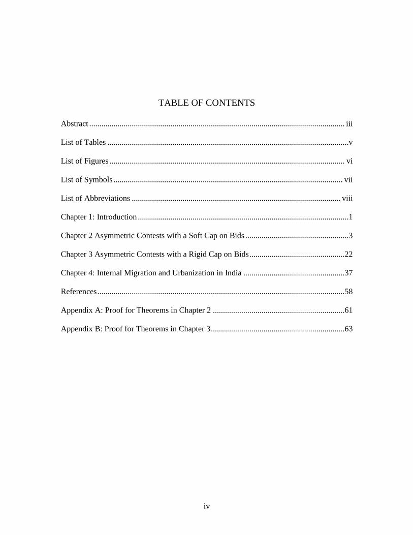
TABLE OF CONTENTS

Abstract .............................................................................................................................. iii

List of Tables .......................................................................................................................v

List of Figures .................................................................................................................... vi

List of Symbols ................................................................................................................. vii

List of Abbreviations ....................................................................................................... viii

Chapter 1: Introduction ........................................................................................................1

Chapter 2 Asymmetric Contests with a Soft Cap on Bids ...................................................3

Chapter 3 Asymmetric Contests with a Rigid Cap on Bids ...............................................22

Chapter 4: Internal Migration and Urbanization in India ..................................................37

References ..........................................................................................................................58

Appendix A: Proof for Theorems in Chapter 2 .................................................................61

Appendix B: Proof for Theorems in Chapter 3 ..................................................................63

v

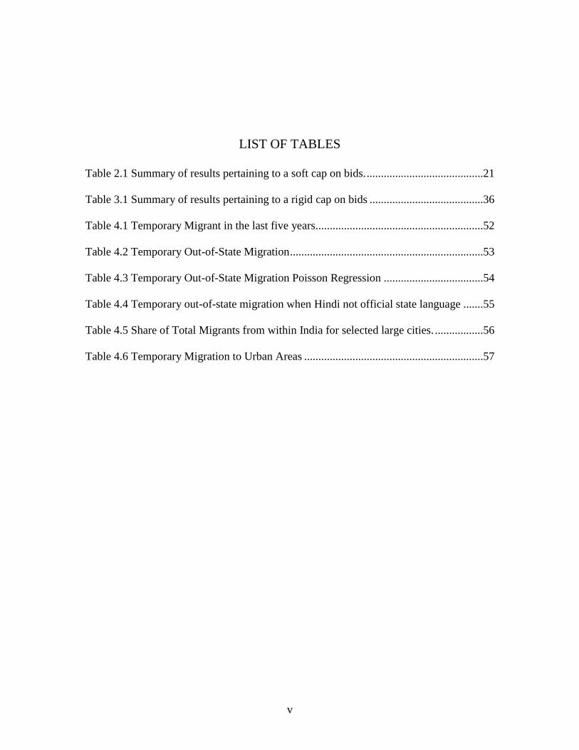
LIST OF TABLES

Table 2.1 Summary of results pertaining to a soft cap on bids. .........................................21

Table 3.1 Summary of results pertaining to a rigid cap on bids ........................................36

Table 4.1 Temporary Migrant in the last five years...........................................................52

Table 4.2 Temporary Out-of-State Migration ....................................................................53

Table 4.3 Temporary Out-of-State Migration Poisson Regression ...................................54

Table 4.4 Temporary out-of-state migration when Hindi not official state language .......55

Table 4.5 Share of Total Migrants from within India for selected large cities. .................56

Table 4.6 Temporary Migration to Urban Areas ...............................................................57

vi

LIST OF FIGURES

Figure 2.1 Cost Functions and Cumulative Distribution Functions ..................................13

Figure 3.1 Cost Functions and Cumulative Distribution Functions ..................................29

Figure 3.2 Cost Functions and Cumulative Distribution Functions ..................................30

Figure 3.3 Aggregate Cost and Aggregate Bids for a Rigid Cap on bids ..........................34

vii

LIST OF SYMBOLS

𝑥𝑖 bid amount for player 𝑖.

𝑉 Value of prize, same for both players.

𝐶𝑖(𝑥) Cost function faced by player 𝑖. Cost is a function of the bid amount 𝑥

𝐿𝑖(𝑥) Cost function faced by player 𝑖 up till the point of discontinuity.

𝐹𝑖 cumulative distribution function for player 𝑖.

𝑠 soft cap on bids, 𝑠 > 0.

𝑚 monetary penalty 𝑚 > 0, or fine imposed on the player who breaches the soft cap.

𝑟 rigid cap on bids, 𝑟 > 0.

viii

LIST OF ABBREVIATIONS

IRR ......................................................................................................... Incident Rate Ratio

NE ............................................................................................................. Nash Equilibrium

RAB ............................................................... Aggregate Bids in case of Rigid Cap on bids

RTC ........................................................................ Total Cost in case of Rigid Cap on bids

SAB .................................................................. Aggregate Bids in case of Soft Cap on bids

STC ........................................................................... Total Cost in case of Soft Cap on bids

1

CHAPTER 1

INTRODUCTION

Contests are events where two or more interested parties or players, compete by

expending effort or resources in order to secure something of value to all players. Contest

can be symmetric, or asymmetric, for a variety of reasons. There could be player specific

attributes that lead one player to have a certain advantage and thereby making the contest

uneven, and asymmetric. In such contests, a cap on bids is placed so as to limit the spending

of the players, so that no player can gain any advantage over the other. There are many

examples of such situations where a cap on spending is implemented with the view of

making the contest fairer. For example, political campaign financing laws in many

countries ensure that the money that any candidate receives to fight an election campaign,

and how much she spends during the campaign is monitored very tightly so that there is no

expenditure that is unaccounted for.

Che and Gale (1998), were perhaps the first to study caps being put in place in a

game theoretic setting of asymmetric contests. Che and Gale (1998) however, considered

a cap which could not be breached by anyone. They showed that the stronger of the two

players in the contest would see her chances of winning this contest to reduce slightly, and

increasing the total cost. Kaplan and Wettstein (2006) pointed out that in most practical

situations, a cap on bids is not one that cannot be breached. An example could be one of

breaching the speed limit while driving. In such cases in the real world, breaching a cap

attracts a fine, monetary or otherwise. Kaplan and Wettstein (2006) show that a contest

2

with no cap on bids stochastically dominates one with cap on bids. We study the three

possible cases here, one with a ‘soft’ cap on bids, which has an associated fine for breaching

the cap, the second case with no cap on bids, and finally one with rigid cap on bids which

cannot be breached. Additionally, we also model the contest in a manner distinct from

earlier approaches in the literature, in that, we allow for players to face discontinuous cost

functions, which competing for a single prize of homogenous valuation. With

discontinuous cost functions, we attempt to capture the jump in cost that a fine, or a

monetary penalty could potentially create if a player were to breach the cap. Alternatively,

a player might factor the jump in cost due to the fine, and bid accordingly.

The third chapter, unlike the first two, which deal with game theoretic models, is

about internal migration and urbanization in India. As India grows economically and also

in terms of its population soon to become the world’s largest, internal migration and

urbanization in India will be of greater interest. I have tried to bring to fore the aspect of

linguistic diversity in India, which is unlike any other country, and how that impact internal

migrations and urbanization. This draws on the cross-country done by Chauvin et. al.

(2017) who find it difficult to explain the low (labor) mobility in India and the high urban

wage premiums there. I attempt to find answers to the questions raised by Chauvin et. al.

(2017) in the linguistic diversity that exists in India. Despite issues pertaining to the

availability of satisfactory data, I am able to show and highlight the impact that linguistic

diversity in India has on internal migration in India.

3

CHAPTER 2

ASYMMETRIC CONTESTS WITH A SOFT CAP ON BIDS

1. Introduction

A cap on spending has conventionally been argued for as a way of providing a level

playing field to contestants of varying capabilities. When the contest is an election

campaign putting a cap on how much a political party, or a candidate can spend on the

campaign is meant to ensure that no one party or candidate accumulates advantage based

simply on their capacity to outspend their opponent(s). Similarly, a cap on salary paid to

players by sports teams is meant to ensure that the best talent is not concentrated in just a

handful of teams making them extraordinarily dominant in a sports league. Usually these

caps are enforced through fines or penalties levied upon those who spend in excess of the

cap. For the 2015 season, the Major League Baseball (MLB) had a spending cap in form

of a Competitive Balance Tax, also known as a Luxury Tax, where a team spending more

than $189 million in player payroll would have to pay a tax for every dollar they were

above the cap1. This however did not prevent Los Angeles Dodgers from spending in

excess of $298 million, significantly above the $189 million cap. LA Dodgers was not

alone in this, they were joined by New York Yankees, Boston Red Sox, and San Francisco

1 Breaking Down Over $400 Million In MLB Luxury Tax Penalties Since 2003. Maury Brown, Forbes, Dec

3, 2015

https://www.forbes.com/sites/maurybrown/2015/12/03/breaking-down-over-400-million-in-mlb-luxury-

tax-penalties-since-2003/#33bb1623541a

4

Giants. Owing to the structure of this Luxury Tax, the amount that these teams had to pay

as a consequence of breaching the cap ranges from $1.3 million for SF Giants to almost

$44 million for LA Dodgers. In the field of politics, ‘Vote Leave’, the official campaign

group advocating British exit from the European Union in the 2016 referendum on that

issue, was fined £61,000 by the (UK) Electoral Commission for breaching the £7 million

spending limit, and spending approximately an extra £500,0002. More recently, soccer’s

European governing body, UEFA, opened investigation into accusations of violation of

Financial Fair Play rules by the English team Manchester City and its owner3. These are

just some of the instances that demonstrate that contestants are willing to exceed a cap on

spending and include the imminent penalty as part of the costs in pursuit of maximizing

their payoffs4.

Given the examples discussed above, it is imperative to point out that there is a

distinction between the cost that players incur in a contest, and the bids they make. The

organizer may want players to incur a high cost in preparing for a contest as a signal of

their intent. For example, in a tendering process for a contract, the organizing party

(government agency or private firm) may want prospective contractors to come up

elaborate proposals for implementation of the project under consideration. This might

increase the cost for the prospective contractors, the organizing party could use the signal

2 Vote Leave fined and referred to police. Jim Pickard and Camilla Hodgson, Financial Times, July 17, 2018

https://www.ft.com/content/a8b848ce-8987-11e8-b18d-0181731a0340 3 Manchester City accuse Uefa of leaks amid Champions League ban threat. David Conn, The Guardian, May

14, 2019

https://www.theguardian.com/football/2019/may/14/manchester-city-uefa-champions-league-ban-protest-

innocence 4 In the case of MLB 2015 season described above, the LA Dodgers spent an extra $109 million above the

cap, which came at a cost of almost $44 million, this shows that costs beyond the threshold of a cap, ‘jumps’

owing to the penalty imposed.

5

to reject those candidates who may come across as tacky. Alternately, in a promotion

contest to be a top executive, a firm might prefer to lower costs for all players and simply

expect that the prospective candidates would put in maximum effort as their bid. This

shows that the distinction between the cost to players (aggregate cost) and bids by players

(aggregate bids) may matter to both the players and the organizer.

2. Literature

Che and Gale (1998) was amongst the first papers to formally analyze model a

contest with caps. They model a contest as a complete information two-player all-pay

auction where players have different valuations for the same prize and their bid is the cost

they incur in participating in the contest. They consider a rigid cap on bids which simply

cannot be breached. As their model considers the cost to be the bid, there is no distinction

between aggregate cost, and aggregate bids. They find that a small rigid cap on bids leads

to an increases in aggregate cost in the contest, which is the same as an increase in

aggregate bids as per their model. Kaplan and Wettstein (2006) in response point out that

more often than not, there is a fine or a penalty associated with the breaching of a cap on

bids, and so a soft, and not a rigid cap is more commonplace. They model the costs incurred

by players as strictly increasing continuous functions of the bid amount. They argue that

bidding without cap stochastically dominates bidding with a (soft) cap, and that the

imposition of a soft cap does not affect aggregate costs but always reduces expected bids.

They further argue that monetary fines could be welfare enhancing, while non-monetary

fines like banning a team may be detrimental. In their response, Che and Gale (2006)

discuss and argue that the aggregate costs increase due cost-equalizing shifts when players

face different cost functions. They further show that monetary fines have no effect on

6

expected aggregate cost, while a nonmonetary penalty generates strictly higher expected

aggregate cost. In a more recent paper, Olszewski and Siegel (2019) look at the effect of

both, rigid and soft caps on the aggregate costs incurred by, and aggregate bids made by

contestants in large all-pay auction contests; where a large number of heterogeneous

contestants compete for a large number of prizes. They conclude that as far as aggregate

costs are concerned, flexible caps have next to no effect, but rigid caps always lower

aggregate costs. Rigid caps also decrease aggregate bids when cost functions are linear or

concave, but could increase aggregate bids for convex cost functions in some conditions.

Flexible caps on the other hand, always decrease aggregate bids. Their approach is different

from the studies mentioned earlier, in that, they consider a situation with 𝑛 number of

players and 𝑛 number of prizes, while earlier studies are 2-player games with a single prize

and 2-valuations of that prize. Furthermore, Olszewski and Siegel (2019) use an assortative

allocation to award 𝑛 prizes to 𝑛 players based on their bid. The authors do have a similarity

with earlier works as each player faces strictly increasing and continuous cost functions

under all circumstances. These studies show there to be some ambiguity around the effects

of a cap on bids5, 6. In this study we focus on soft cap on bids, where a monetary penalty is

implemented for breaching a cap on bids. Our study sits well with the discussion initiated

by Che and Gale (1998) and carried forward by Kaplan and Wettstein (2006), and Che and

Gale (2006). Our findings support Kaplan and Wettstein (2006) when they say that bidding

without a cap strictly dominates bidding with a soft cap on bids. We further are in

5 Pastine and Pastine (2013) extended Kaplan and Wettstein (2006) and Che and Gale (2006) by incorporating

politician preferences into their framework. 6 Other studies look at the Caps in Contests from different angles. Gavious, Moldovanu, and Sela (2002)

study private-information contests with caps. Szech (2015) revisits Che and Gale (1998) and analyzes

different tie-breaking rules.

7

agreement with Kaplan and Wettstein (2006), and Olszewski and Siegel (2019), in so far

as the decrease in aggregate bids is concerned when a soft cap in implemented. However,

we show that aggregate costs decrease when a soft cap with a monetary fine is

implemented, while both, Kaplan and Wettstein (2006), and Olszewski and Siegel (2019),

argue that a soft cap has no effect on aggregate costs. These results are highlighted in Table

1.1.

We model an asymmetric contest as an all-pay auction where the players have the

same valuation of the prize, but different right-continuous cost functions. In doing so, we

seek to capture the ‘jump’, or the discontinuity in the costs owing to a non-rigid fine or a

soft cap being implemented.

It is standard in the literature to model asymmetric contests as all-pay auctions

where players have different valuation of a single prize and the same linear cost functions,

and to obtain conventional mixed-strategy equilibria, where the most efficient player

obtains a positive expected payoff, and the other players get expected zero payoffs. See,

for example, Hillman and Riley (1989), Baye, Kovenock, and De Vries (1993, 1996).7 A

typical assumption in this literature is that cost functions are twice continuously

differentiable.

We provide sufficient conditions for uniqueness of the conventional mixed-strategy

equilibrium in our setting. This equilibrium is qualitatively different from equilibria in

previous studies. Moreover, we construct the conventional mixed-strategy equilibrium

even if different players have caps at different points and the number of such caps is finite.

7 Siegel (2009, 2010, 2014) considers general contests with continuous cost functions.

8

First, we analyze two-player asymmetric contests. We show that there exists the

conventional mixed-strategy equilibrium. However, there might be pure-strategy equilibria

in our model, if the assumption about the right-continuity of the cost functions is violated,

Example 2 illustrates that situation.

3. Asymmetric Two-Player Contest with a Soft Cap

Suppose that two players contest a single prize 𝑉 > 0. The prize value is same for

both players, but the players’ cost functions, indicating their ability, can be different. Thus

we have an asymmetric contest.

We define a ‘soft’ cap on bids as the maximum bid permissible with a penalty

imposed on any player who bids in excess of the soft cap. Essentially, a soft cap on bids is

one where a player can bid in excess of the cap, but at an additional cost incurred in terms

of a monetary penalty or fine. Each player 𝑖 can bid a positive amount 𝑥𝑖 < 𝑠, where 𝑠 > 0

is the soft cap on bids. For a bid 𝑥𝑖 ≥ 𝑠, player 𝑖 will be penalized and will have to pay a

fixed monetary fine 𝑚 ≥ 0. The imposition of the monetary fine will have the effect of

creating a ‘jump’ in the cost faced by any player. Essentially, the cost function faced by

player 𝑖 will increase continuously as long as 𝑥𝑖 < 𝑠. For 𝑥𝑖 ≥ 𝑠 however, the cost function

would be displaced vertically upwards, or jump up by 𝑚 ≥ 0. We model this asymmetric

contest with a soft cap on bids below.

We assume that players have right-continuous cost functions with at most one

discontinuity which satisfy the following conditions8

8 We will discuss left-continuous cost functions below.

9

𝐶𝑖(𝑥) = {

𝐿𝑖(𝑥), if 𝑥 < 𝑠,

𝐿𝑖(𝑥) + 𝑚, if 𝑥 ≥ 𝑠,

(1)

where,

𝑚 ≥ 0 (2)

𝐿1(0) = 𝐿2(0) = 0 (3)

𝐿𝑖(𝑥) is strictly increasing functions for 𝑖 = 1, 2, (4)

We assume that there exists 0 < 𝑡𝑖 < ∞ such that

𝐶𝑖(𝑡𝑖) = 𝑉 for 𝑖 = 1, 2, (5)

and

𝑡2 ≤ 𝑡1. (6)

based on which, we call Player 1 more efficient player.

Each player 𝑖 exerts effort 𝑥𝑖 ≥ 0 in order to win the prize in the all-pay auction

and obtains the following payoff

𝑢𝑖(𝑥1, 𝑥2) =

{

−𝐶𝑖(𝑥𝑖) , if 𝑥𝑖 < 𝑥−𝑖,

𝑉

2− 𝐶𝑖(𝑥𝑖) , if 𝑥1 = 𝑥2,

𝑉 − 𝐶𝑖(𝑥𝑖) , if 𝑥𝑖 > 𝑥−𝑖.

(7)

We can describe a mixed-strategy equilibrium in our setting now.

10

Theorem 1. If conditions (1) – (6) hold, and 𝑑 < 𝑡2, then there exists a conventional mixed-

strategy NE in the asymmetric two-player contest, where Player 1 randomizes according

to the following cumulative distribution function

𝐹1(𝑥) =1

𝑉𝐶2(𝑥), (8)

on the interval [0, 𝑡2] placing an atom at 𝑥 = 𝑠, if 𝑠 < 𝑡2; and player 2 randomizes

according to the following cumulative distribution function, and Player 2 randomizes

according to the following cumulative distribution function

𝐹2(𝑥) =𝑉 − 𝐶1(𝑡2)

𝑉+1

𝑉𝐶1(𝑥), (9)

on the interval [0, 𝑡2] placing an atom at zero and at 𝑥 = 𝑠 if 𝑠 < 𝑡2.

Note that if 𝑚 = 0, or there is no penalty gap, then we get a conventional mixed-

strategy NE, similar to the mixed-strategy equilibrium in Hillman and Riley (1989), and in

Baye, Kovenock, and De Vries (1996).

Corollary 1. If 𝑚 = 0 and conditions (3) – (6) hold, then there exists a conventional mixed-

strategy NE in the asymmetric two-player contest, where player 1 randomizes according

to the following cumulative distribution function

Player 1 randomizes according to the following cumulative distribution function

𝐹1(𝑥) =1

𝑉𝐶2(𝑥)

on the interval [0, 𝑡2], and Player 2 randomizes according to the following cumulative

distribution function

11

𝐹2(𝑥) =𝑉 − 𝐶1(𝑡2)

𝑉+1

𝑉𝐶1(𝑥)

on the interval [0, 𝑡2], placing an atom of size at zero.

The following corollary is a well-known result in the contest literature where cost

functions are linear.

Corollary 2. If 𝑚 = 0, and

𝐶1(𝑥) = 𝐶2(𝑥) = 𝑥,

then there exists a unique (conventional) mixed-strategy NE in the symmetric two-player

contest, where both players randomize according to the following cumulative distribution

function

𝐹1(𝑥) = 𝐹2(𝑥) =𝑥

𝑉

on the interval [0, 𝑡2].

If 𝑚 > 0 and 𝑠 < 𝑡2, then mass points appear at 𝑥 = 0 for player 2 and at the point

of discontinuity, 𝑥 = 𝑠, for both players in the conventional mixed-strategy NE. Note that

player 1 (2) cannot take advantage of the mass point at 𝑥 = 𝑠 in the cdf of player 2 (1)

because her own cost is discontinuous exactly at that point. The following example

illustrates Theorem 1.

Example 1. Suppose that 𝑉 = 2, 𝑠 = 1, 𝑚 = 0.5, the cost functions are

𝐶1(𝑥) = {

√𝑥, if 𝑥 < 1,

√𝑥 + 0.5, if 𝑥 ≥ 1,

and

12

𝐶2(𝑥) = {

𝑥, if 𝑥 < 1,

𝑥 + 0.5, if 𝑥 ≥ 1.

Then, 𝑡2 = 1.5 < 2.25 = 𝑡1 and conditions (1) – (6) hold. In the conventional mixed-

strategy NE, player 1 randomizes according to the following cumulative distribution

function:

𝐹1(𝑥) =

{

1

2𝑥, if 𝑥 ∈ [0, 1),

1

2𝑥 +

1

4, if 𝑥 ∈ [1, 1.5],

on the interval [0, 1.5] placing an atom of size 1

4 at one. Player 2 randomizes according to

the following cumulative distribution function

𝐹2(𝑥) =

{

1.5 − √1.5

2+1

2√𝑥, if 𝑥 ∈ [0, 1)

2 − √1.5

2+1

2√𝑥, if 𝑥 ∈ [1, 1.5]

on the interval [0, 1.5], placing an atom of size 1

4 at one and an atom of size (

1.5−√1.5

2) at

zero.

Figure 2.1 below shows the cost functions used in this example on the left-hand

side panel while the cumulative distribution functions calculated above are plotted on the

right-hand side panel. The solid line represents Player 1’s cost function and cumulative

distribution function in the respective panels, while the dotted line represents the same for

Player 2 in the respective panels.

13

Figure 2.1 Cost Functions and Cumulative Distribution Functions

𝐶1(𝑥) – solid line and 𝐶2(𝑥) – dash line on the left panel

𝐹1(𝑥) – solid line and 𝐹2(𝑥) – dash line on the right panel

Next, we establish uniqueness of the conventional mixed-strategy NE in the

asymmetric two-player contest.

Theorem 2 If conditions (1) – (6) hold, then the conventional mixed-strategy equilibrium

is a unique NE in the asymmetric two-player contest.

The proof is standard and similar to the proofs of Propositions 1 and 2 in Hillman

and Riley (1989) and thus is omitted. The following example shows that there can be a

pure-strategy NE if cost functions are left-continuous, or assumption (1) is violated.

Example 2. Suppose that 𝑉 = 1, 𝑠 = 0.1, and 𝑚 = 0.9, and

𝐶1(𝑥) = 𝐶2(𝑥) = {

0.1𝑥, if 𝑥 ∈ [0, 0.1],

0.1𝑥 + 0.9, if 𝑥 ∈ (0.1, 1],

Then, 𝑡2 = 1 = 𝑡1, and conditions (2) – (6) hold.

Note that there exists a pure strategy equilibrium where both players bid

14

𝑥1 = 𝑥2 = 0.1

and obtain expected payoffs

𝐸𝜋𝑖(0.1, 0.1) = 0.5 − 0.01 = 0.49, for 𝑖 = 1, 2.

3.1 Aggregate Bids and Total Cost

Having determined the bidding behavior for the two players, we now focus on the

total cost in the asymmetric two-player contest with a soft cap. As discussed earlier, the

total cost, and the expected aggregate bids, as given below, are also important aspects of

an asymmetric contest.

𝑆𝑇𝐶 = ∫ 𝐶1(𝑥)𝑡2

0

𝑑𝐹1(𝑥) + ∫ 𝐶2(𝑥)𝑡2

0

𝑑𝐹2(𝑥),

and the expected aggregate bids

𝑆𝐴𝐵 = ∫ 𝑥𝑡2

0

𝑑𝐹1(𝑥) + ∫ 𝑥𝑡2

0

𝑑𝐹2(𝑥).

From Theorem 1,

∫ 𝐶1(𝑥)𝑡2

0

𝑑𝐹1(𝑥) =

{

1

𝑉∫ 𝐿1(𝑥)𝑡2

0

𝑑𝐿2(𝑥), 𝑖𝑓 𝑡2 < 𝑠,

1

𝑉∫ 𝐿1(𝑥)𝑠

0

𝑑𝐿2(𝑥) +1

𝑉∫ (𝐿1(𝑥)𝑡2

𝑠

+𝑚) 𝑑𝐿2(𝑥), 𝑖𝑓 𝑡2 ≥ 𝑠,

(10)

and

∫ 𝐶2(𝑥)𝑡2

0

𝑑𝐹2(𝑥) =

{

1

𝑉∫ 𝐿2(𝑥)𝑡2

0

𝑑𝐿1(𝑥), 𝑖𝑓 𝑡2 < 𝑠,

1

𝑉∫ 𝐿2(𝑥)𝑠

0

𝑑𝐿1(𝑥) +1

𝑉∫ (𝐿2(𝑥)𝑡2

𝑠

+𝑚) 𝑑𝐿1(𝑥), 𝑖𝑓 𝑡2 ≥ 𝑠.

(11)

15

Therefore, we get the following result.

Theorem 3 The total cost is

𝑆𝑇𝐶 =

{

𝐶1(𝑡2), 𝑖𝑓 𝑡2 < 𝑠

𝐶1(𝑡2) −𝑚

𝑉(𝐿1(𝑠) + 𝐿2(𝑠) + 𝑚), 𝑖𝑓 𝑡2 ≥ 𝑠

(12)

The total cost is maximized, if there is no soft cap, or 𝑚 = 0. The expected aggregate bids

are independent from the soft cap,

𝑆𝐴𝐵 =1

𝑉(𝑡2(𝐿1(𝑡2) + 𝐿2(𝑡2)) − (∫ 𝐿1(𝑥)𝑑𝑥

𝑡2

0

+∫ 𝐿2(𝑥)𝑑𝑥𝑡2

0

)) . (13)

The following example illustrates the theorem.

Example 3. Suppose that 𝑉 = 2, 𝑚 = 0, 𝐶1(𝑥) = √𝑥, and 𝐶2(𝑥) = 𝑥.

Then, 𝑡2 = 2 < 4 = 𝑡1 and conditions (1) – (6) hold. From Corollary 2, in the conventional

mixed-strategy NE, Player 1 randomizes according to the following cumulative

distribution function

𝐹1(𝑥) =1

2𝑥,

on the interval [0, 2], and Player 2 randomizes according to the following cumulative

distribution function

𝐹2(𝑥) =2 − √2

2+1

2√𝑥

on the interval [0, 2], placing an atom of size (2−√2

2) at zero. From (12), the total cost is

𝑆𝑇𝐶 = 𝐶1(𝑡2) = √2 ≈ 1.41.

16

From (13), the expected aggregate bids are

𝑆𝐴𝐵 =1

𝑉(∫ 𝑥

𝑡2

0

𝑑𝐿2(𝑥) + ∫ 𝑥𝑡2

0

𝑑𝐿1(𝑥))

=1

𝑉(𝑡2(𝐿1(𝑡2) + 𝐿2(𝑡2)) − (∫ 𝐿1(𝑥)𝑑𝑥

𝑡2

0

+∫ 𝐿2(𝑥)𝑑𝑥𝑡2

0

))

𝑆𝐴𝐵 =1

2(2(√2 + 2) − (

2

32(32) +

22

2)) ≈ 1.47.

Now, suppose that a soft cap is introduced. From Example 1, 𝑚 = 0.5, and 𝑠 = 1,

𝐶1(𝑥) = {

√𝑥, if 𝑥 < 1,

√𝑥 + 0.5, if 𝑥 ≥ 1,

and

𝐶2(𝑥) = {

𝑥, if 𝑥 < 1,

𝑥 + 0.5, if 𝑥 ≥ 1.

Then, 𝑡2 = 1.5 < 2.25 = 𝑡1. and conditions (1) – (6) hold. In the conventional mixed-

strategy NE, Player 1 randomizes according to the following cumulative distribution

function

𝐹1(𝑥) =

{

1

2𝑥, if 𝑥 ∈ [0, 1),

1

2𝑥 +

1

4, if 𝑥 ∈ [1, 1.5],

17

on the interval [0, 1.5] placing an atom of size 1

4 at one. Player 2 randomizes according to

the following cumulative distribution function

𝐹2(𝑥) =

{

1.5 − √1.5

2+1

2√𝑥, if 𝑥 ∈ [0, 1),

2 − √1.5

2+1

2√𝑥, if 𝑥 ∈ [1, 1.5],

on the interval [0, 1.5], placing an atom of size 1

4 at 1 and an atom of size (

1.5−√1.5

2) at zero.

From (12), the total cost is

𝑆𝑇𝐶 = 𝐶1(𝑡2) −𝑚

𝑉(𝐿1(𝑠) + 𝐿2(𝑠) +𝑚),

𝑆𝑇𝐶 = √1.5 + 0.5 −0.5

2(1 + 1 + 0.5) ≈ 1.10.

From (13), the expected aggregate bids are

𝑆𝐴𝐵 =1

𝑉(∫ 𝑥

𝑡2

0

𝑑𝐿2(𝑥) + ∫ 𝑥𝑡2

0

𝑑𝐿1(𝑥))

=1

𝑉(𝑡2(𝐿1(𝑡2) + 𝐿2(𝑡2)) − (∫ 𝐿1(𝑥)𝑑𝑥

𝑡2

0

+∫ 𝐿2(𝑥)𝑑𝑥𝑡2

0

))

𝑆𝐴𝐵 =1

2(1.5(1.5 + √1.5) − (

2

31.5(

32) +

1.52

2)) ≈ 0.87.

Note here that both, the total cost and aggregate bids decrease when a soft cap is

introduced.

18

4. Conclusions

We have shown that a two player asymmetric contest can be modeled as one where

the players have the same valuation of the prize, but face different cost functions. This

provides an additional approach to modeling such contests compared to the existing

approach in the literature. The consistency of our results with those in the existing literature

show that our approach is viable and is successful in presenting an additional framework.

Additionally, the introduction of discontinuous cost functions in the model, and using them

capture the ‘jump’ in costs that a player would face when there is a penalty imposed on

breaching a certain spending limit, is another contribution to the literature.

Using our model, we have also explored the various policy options around the

imposition of an exogenous cap on bids, which organizers face when conducting such

contests. We consider the impact such policy has on the total cost to the players and

aggregate bids made by them. We show that, in terms of increasing the total cost faced by

the players, a policy of no cap on bids strictly dominates the one with a soft cap on bids

with a penalty for breaching the cap. While Kaplan and Wettstein (2006), and Olszewski

and Siegel (2019) show that a soft cap has no effect on total cost; Che and Gale (2006)

show an increase in total cost for a soft cap with non-monetary penalties. Our findings on

the other hand, show that implementing a soft cap on bids would decrease the total cost

faced by the players. We believe that our findings are more intuitive as discussed below.

On expected aggregate bids made by players, Example 3 shows that, the aggregate

bids reduce upon the implementation of a soft cap on bids. Our findings, in the context of

19

aggregate bids, support those of Kaplan and Wettstein (2006), and Olszewski and Siegel

(2019).

A. Cap on bids and competition

While analyzing various policies regarding caps on bids in an asymmetric contest,

it may be fruitful to generally consider the effect of such policies on how competitive they

may, or may not, make the contest itself. With there being no cap on bids, the most efficient

(advantaged) player has a clear advantage. Such players may be advantaged in terms of

certain reputational, experiential, or financial factors. This would provide the less efficient

player with few incentives to bid high, knowing this, the most efficient player will also not

bid as high as they could have. There is nonetheless, still a non-zero possibility that the less

efficient player could bid high and catch the most efficient player unaware and win the

contest. However, when a policy of a soft cap on bids is implemented, so that any player

who bids above a certain capped amount would be required to pay a monetary fine, then

only the most efficient player would take that the opportunity to bid close to the cap, or

even breach the cap. The less efficient player would have less inclination to bid close to

the capped amount where they could lose to the more efficient player(s); and have even

less of a proclivity to breach the cap. Knowing this, even the more efficient player(s) would

then not bid large amounts. As a consequence, both, the expected aggregate bids and the

total cost, which is a function of the bids, would therefore decrease in this situation

compared to the policy of no cap on bids, where the less efficient player(s) does not need

to contend with the possibility of an imminent penalty upon bidding in excess of a specific

amount.

20

B. Total Cost and Aggregate Bids

As has been discussed earlier in the introduction, total cost and aggregate bids may

be of interest to both organizers and player. We have shown the effect that a soft cap on

bids has on the two. Our results imply that if an organizer would want to lower the cost to

players, then they should implement a soft cap on bids, that however, would lead to a

decrease in expected aggregate bids. On the other hand, if an organizer would like to

increase aggregate bids, then going for a no cap on bids option would be her choice, that

however, maximizes the total cost for the players or the participants.

21

Table 2.1 Summary of results pertaining to a soft cap on bids.

This table summarizes our findings with regards to soft cap on bids, and compares it with

previous literature on this subject.

Che and

Gale

(1998)

Kaplan and

Wettstein

(2006)

Che and Gale

(2006)

Olszewski

and Siegel

(2019)

This paper

Effect on Aggregate Cost

Soft Cap -- No Effect

Monetary

fine: No

Effect

Nonmonetary

penalty:

Increases

No Effect Decreases

No Cap -- -- -- -- Dominates

Effect on Aggregate Bids

Soft Cap -- Decreases -- Decreases Decreases

No Cap -- Dominates -- -- Dominates

22

CHAPTER 3

ASYMMETRIC CONTESTS WITH A RIGID CAP ON BIDS

1. Introduction

The costs in a contest such as a lobbying or a political campaign can be substantially

high at times, where the contestants can be spending large sums in order to win the contest.

This has been quite apparent in election campaigns in the United States, where the costs of

running a campaign has been increasing over the years. Such increase in campaign

spending can be quite wasteful, as it would require a politician to considerably increase

fund-raising efforts, which may come at cost of other significant activities. Additionally, a

donor could appropriate undue influence on electoral outcomes, or on policy positions by

making a large enough campaign contribution (Che and Gale, 1998). Such situations may

also give one contestant, an undue advantage over another. Similar situations could also

exit in the field of professional team sports. A team may be able to significantly outspend

another, and thereby purchase many extremely expensive players, potentially giving them

extraordinary advantage over other teams. Despite such a variety of scenarios, a cap on

spending has conventionally been argued for as a way of providing a level playing field to

contestants of varying capabilities. In this paper we consider a two-player asymmetric

contest with a single prize. A rigid cap is placed on the amount that the players can bid.

In addition to their being contestants, contests also tend to have other interested

parties whom we may call organizer(s). It is possible, that the organizer(s) might desire for

23

the contestants to incur a high cost in preparation for a contest. The organizer might use

the cost incurred by the contestant as a signal of their intent. A firm wanting to build its

new corporate office might prefer various architecture firms in competition for the project,

to be as elaborate and detailed in their plans and designs for the new corporate office.

Conversely, the organizer might want contestants to incur as low a cost as possible in

preparation for a contest, but would prefer the contestants to expend maximum effort

during the contest. This is the distinction between aggregate cost, that contestants incur in

participating in the contest, and aggregate bids which is the amount or effort that players

expend as they compete.

2. Literature

Che and Gale (1998) was amongst the first papers to formally analyze model a

contest with caps. They model a contest as a complete information two-player all-pay

auction where players have different valuations for the same prize and their bid is the cost

they incur in participating in the contest. They consider a rigid cap on bids which simply

cannot be breached. As their model considers the cost to be the bid, there is no distinction

between aggregate cost, and aggregate bids. They find that a small rigid cap on bids leads

to an increases in aggregate cost in the contest, which is the same as an increase in

aggregate bids as per their model. Kaplan and Wettstein (2006) in response point out that

more often than not, there is a fine or a penalty associated with the breaching of a cap on

bids, and so a soft, and not a rigid cap is more commonplace. They model the costs incurred

by players as strictly increasing continuous functions of the bid amount. They argue that

bidding without cap stochastically dominates bidding with a (soft) cap, and that the

imposition of a soft cap does not affect aggregate costs but always reduces expected bids.

24

They further argue that monetary fines could be welfare enhancing, while non-monetary

fines like banning a team may be detrimental. In their response, Che and Gale (2006)

discuss and argue that the aggregate costs increase due cost-equalizing shifts when players

face different cost functions. They further show that monetary fines have no effect on

expected aggregate cost, while a nonmonetary penalty generates strictly higher expected

aggregate cost. In a more recent paper, Olszewski and Siegel (2019) look at the effect of

both, rigid and soft caps on the aggregate costs incurred by, and aggregate bids made by

contestants in large all-pay auction contests; where a large number of heterogeneous

contestants compete for a large number of prizes. They conclude that as far as aggregate

costs are concerned, flexible caps have next to no effect, but rigid caps always lower

aggregate costs. Rigid caps also decrease aggregate bids when cost functions are linear or

concave, but could increase aggregate bids for convex cost functions in some conditions.

Flexible caps on the other hand, always decrease aggregate bids. Their approach is different

from the studies mentioned earlier, in that, they consider a situation with 𝑛 number of

players and 𝑛 number of prizes, while earlier studies are 2-player games with a single prize

and 2-valuations of that prize. Furthermore, Olszewski and Siegel (2019) use an assortative

allocation to award 𝑛 prizes to 𝑛 players based on their bid. The authors do have a similarity

with earlier works as each player faces strictly increasing and continuous cost functions

under all circumstances. These studies show there to be some ambiguity around the effects

of a cap on bids9, 10. In this study we focus on rigid cap on bids, that cannot be breached.

9 Pastine and Pastine (2013) extended Kaplan and Wettstein (2006) and Che and Gale (2006) by incorporating

politician preferences into their framework. 10 Other studies look at the Caps in Contests from different angles. Gavious, Moldovanu, and Sela (2002)

study private-information contests with caps. Szech (2015) revisits Che and Gale (1998) and analyzes

different tie-breaking rules.

25

Our study sits well with the discussion initiated by Che and Gale (1998) and carried

forward by Kaplan and Wettstein (2006), and Che and Gale (2006). Our findings support

Kaplan and Wettstein (2006) when they say that bidding without a cap strictly dominates

bidding with a soft cap on bids. We further are in agreement with Kaplan and Wettstein

(2006), and Olszewski and Siegel (2019), in so far as the decrease in aggregate bids is

concerned when a soft cap in implemented. However, we show that aggregate costs

decrease when a soft cap with a monetary fine is implemented, while both, Kaplan and

Wettstein (2006), and Olszewski and Siegel (2019), argue that a soft cap has no effect on

aggregate costs. These results are highlighted in Table 1.

We model an asymmetric contest as an all-pay auction where the players have the

same valuation of the prize, but different right-continuous cost functions. In doing so, we

seek to capture the ‘jump’, or the discontinuity in the costs owing to a non-rigid fine or a

soft cap being implemented.

It is standard in the literature to model asymmetric contests as all-pay auctions

where players have different valuation of a single prize and the same linear cost functions,

and to obtain conventional mixed-strategy equilibria, where the most efficient player

obtains a positive expected payoff, and the other players get expected zero payoffs. See,

for example, Hillman and Riley (1989), Baye, Kovenock, and De Vries (1993, 1996).11 A

typical assumption in this literature is that cost functions are twice continuously

differentiable.

11 Siegel (2009, 2010, 2014) considers general contests with continuous cost functions.

26

We provide sufficient conditions for uniqueness of the conventional mixed-strategy

equilibrium in our setting. This equilibrium is qualitatively different from equilibria in

previous studies. Moreover, we construct the conventional mixed-strategy equilibrium

even if different players have caps at different points and the number of such caps is finite.

First, we analyze two-player asymmetric contests. We show that there exists the

conventional mixed-strategy equilibrium. However, there might be pure-strategy equilibria

in our model, if the assumption about the right-continuity of the cost functions is violated,

Example 2 illustrates that situation.

3. Asymmetric Two-Player Contest with a Rigid Cap

We will consider a rigid cap on bids now. We define a ‘rigid’ cap on bids as the

maximum bid permissible. Each player 𝑖 can bid a positive amount 𝑥𝑖 ≤ 𝑟 in the contest,

where 𝑟 > 0 is the rigid cap on bids. Suppose that two players contest a prize 𝑉 > 0. The

value of the prize is same for both players, but the players’ cost functions can be different

and satisfy the following conditions

𝐿1(𝑥) ≤ 𝐿2(𝑥), (1)

with,

𝐿1(0) = 𝐿2(0) = 0 (2)

𝐿𝑖(𝑥) is strictly increasing functions for 𝑖 = 1, 2, (3)

We assume that there exists 0 < 𝑡𝑖 < ∞ such that

𝐿𝑖(𝑡𝑖) = 𝑉 for 𝑖 = 1, 2, (4)

27

and

𝑡2 ≤ 𝑡1. (5)

based on which, we call Player 1 more efficient player.

Each player 𝑖 exerts effort 𝑥𝑖 ≥ 0 in order to win the prize in the all-pay auction

and obtains the following payoff

𝑢𝑖(𝑥1, 𝑥2) =

{

−𝐿𝑖(𝑥𝑖) , if 𝑥𝑖 < 𝑥−𝑖,

𝑉

2− 𝐿𝑖(𝑥𝑖) , if 𝑥1 = 𝑥2,

𝑉 − 𝐿𝑖(𝑥𝑖) , if 𝑥𝑖 > 𝑥−𝑖.

(6)

In this setting, where (1) – (6) hold, and

𝑟 < 𝑡2. (7)

3.1 Small Rigid Cap

It is intuitively clear that both players make every possible effort if the rigid cap on

bids is small enough. Denote

𝑟0 = 𝑚𝑖𝑛 {𝐿1−1 (

𝑉

2) , 𝐿2

−1 (𝑉

2)} = 𝐿2

−1 (𝑉

2) < 𝑡2. (8)

We get the following result,

Theorem 1 if conditions (1) – (5) and

0 < 𝑟 ≤ 𝑟0 (9)

28

hold, then there exists a pure-strategy NE in which each player submits a bid of r in the

asymmetric two-player contest with a rigid cap.

3.2 Large Rigid Cap

Suppose the rigid cap 𝑟, is “large”, and given as

𝑟0 < 𝑟 < 𝑡2. (10)

It is obvious here that both players cannot bid the cap level in an equilibrium as at least one

of them will get a negative payoff. We can describe the mixed-strategy in our setting now.

Theorem 2 If conditions (1) – (5), and (10) hold, then there exists a mixed-strategy NE in

the asymmetric two-player contest with a rigid cap, 𝑟, where Player 1 randomizes

according to the following cumulative distribution function.

𝐻1(𝑥) =1

𝑉𝐿2(𝑥), (11)

on the interval [0, 𝑡] placing an atom at 𝑥 = 𝑟; and Player 2 randomizes according to the

following cumulative distribution function

𝐻2(𝑥) =𝑉 − (2𝐿1(𝑟) − 𝐿1(𝑡))

𝑉+1

𝑉𝐿1(𝑥), (12)

on the interval [0, 𝑡], placing an atom at zero and at 𝑥 = 𝑟. Where

𝑡 = 𝐿2−1(2𝐿2(𝑟) − 𝑉) (13)

Consider the following example

Example 1. Suppose that 𝑉 = 1, 𝐿1(𝑥) =1

2𝑥, and 𝐿2(𝑥) = 𝑥.

29

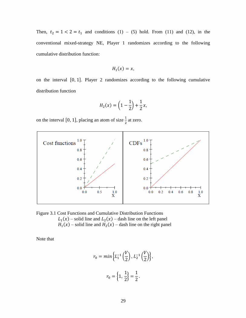
Then, 𝑡2 = 1 < 2 = 𝑡1 and conditions (1) – (5) hold. From (11) and (12), in the

conventional mixed-strategy NE, Player 1 randomizes according to the following

cumulative distribution function:

𝐻1(𝑥) = 𝑥,

on the interval [0, 1]. Player 2 randomizes according to the following cumulative

distribution function

𝐻2(𝑥) = (1 −1

2) +

1

2𝑥,

on the interval [0, 1], placing an atom of size 1

2 at zero.

Figure 3.1 Cost Functions and Cumulative Distribution Functions

𝐿1(𝑥) – solid line and 𝐿2(𝑥) – dash line on the left panel

𝐻1(𝑥) – solid line and 𝐻2(𝑥) – dash line on the right panel

Note that

𝑟0 = 𝑚𝑖𝑛 {𝐿1−1 (

𝑉

2) , 𝐿2

−1 (𝑉

2)} ,

𝑟0 = {1, 1

2} =

1

2 .

30

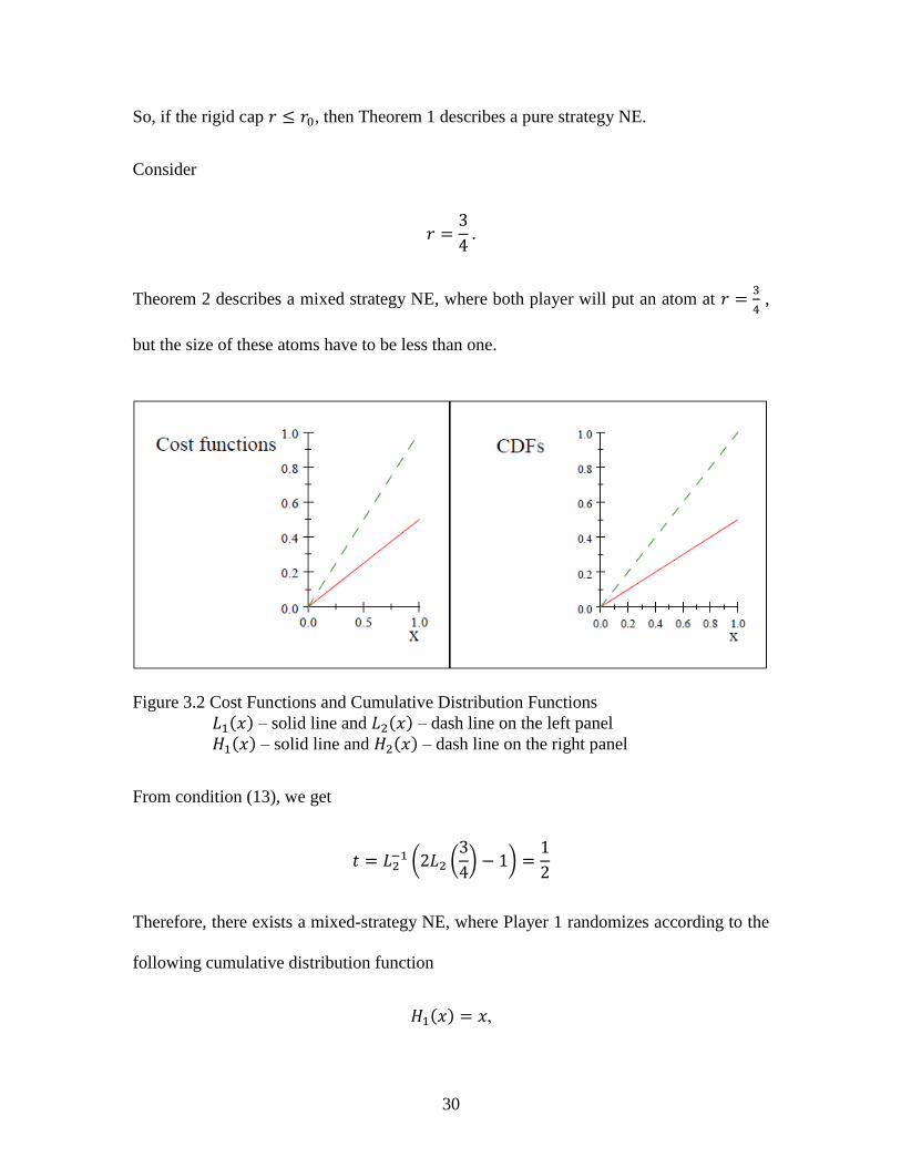
So, if the rigid cap 𝑟 ≤ 𝑟0, then Theorem 1 describes a pure strategy NE.

Consider

𝑟 =3

4 .

Theorem 2 describes a mixed strategy NE, where both player will put an atom at 𝑟 =3

4 ,

but the size of these atoms have to be less than one.

Figure 3.2 Cost Functions and Cumulative Distribution Functions

𝐿1(𝑥) – solid line and 𝐿2(𝑥) – dash line on the left panel

𝐻1(𝑥) – solid line and 𝐻2(𝑥) – dash line on the right panel

From condition (13), we get

𝑡 = 𝐿2−1 (2𝐿2 (

3

4) − 1) =

1

2

Therefore, there exists a mixed-strategy NE, where Player 1 randomizes according to the

following cumulative distribution function

𝐻1(𝑥) = 𝑥,

31

on the interval [0,1

2] placing an atom at 𝑥 = 𝑟 =

3

4 ; and Player 2 randomizes according to

the following cumulative distribution function

𝐻2(𝑥) =1

2+1

2𝑥,

on the interval [0,1

2], placing an atom of size

1

2 at zero and at 𝑥 = 𝑟 =

3

4 .

3.3 Aggregate Bids and Total Cost

We can now determine the total cost in the asymmetric two-player contest with a

rigid cap

𝑅𝑇𝐶(𝑟) = ∫ 𝐿1(𝑥)𝑟

0

𝑑𝐻1(𝑥) + ∫ 𝐿2(𝑥)𝑟

0

𝑑𝐻2(𝑥),

and the expected aggregate bids

𝑅𝐴𝐵(𝑟) = ∫ 𝑥𝑟

0

𝑑𝐻1(𝑥) + ∫ 𝑥𝑟

0

𝑑𝐻2(𝑥).

For both the expressions above, the first term gives the total cost (or expected

aggregate bids) for Player 1, and the second term gives the same for Player 2.

3.3.1 Small Rigid Cap

Suppose that condition (9) holds, then

𝑅𝑇𝐶(𝑟) = 𝐿1(𝑟) + 𝐿2(𝑟),

and

𝑅𝐴𝐵(𝑟) = 2𝑟.

32

The total cost and the expected aggregate bids are maximized at 𝑟 = 𝑟0, or

max0≤𝑟≤𝑟0

𝑅𝑇𝐶(𝑟) = 𝐿1(𝑟0) + 𝐿2(𝑟0) ,

and

max0≤𝑟≤𝑟0

𝑅𝐴𝐵(𝑟) = 2𝑟0 .

3.3.2 Large Rigid Cap

Suppose that condition (10) holds, then we get the following result.

Theorem 3 The total costs are

𝑅𝑇𝐶(𝑟) = {

𝐿1(𝑟) + 𝐿2(𝑟), 𝑖𝑓 0 < 𝑟 ≤ 𝑟0 < 𝑡2,

2𝐿1(𝑟) − 𝐿1(𝑡), 𝑖𝑓 𝑟0 < 𝑟 < 𝑡2,

(14)

and the aggregate bids are

𝑅𝐴𝐵(𝑟) =

{

2𝑟, 𝑖𝑓 0 < 𝑟 ≤ 𝑟0 < 𝑡2,

1

𝑉(𝑡(𝐿1(𝑡) + 𝐿2(𝑡)) − ∫ (𝐿1(𝑥) + 𝐿2(𝑥))𝑑𝑥

𝑡

0

)

+ 𝑟(2 − 𝐻1(𝑡) − 𝐻2(𝑡)), 𝑖𝑓 𝑟0 < 𝑟 < 𝑡2

(15)

where 𝑡 is defined in (13).

The following examples illustrates.

Example 2. Suppose that 𝑉 = 10, 𝐿1(𝑥) = 𝑥 ≤ 2𝑥 = 𝐿2(𝑥).

Then

𝑡2 = 5 < 10 = 𝑡1,

33

𝑟0 = 𝐿2−1 (

𝑉

2) = 2.5,

and

𝑡 = 𝐿2−1(2𝐿2(𝑟) − 𝑉) = 2𝑟 − 5.

The total cost is then given as

𝑅𝑇𝐶(𝑟) = {

3𝑟, 𝑖𝑓 0 < 𝑟 ≤ 2.5,

5, 𝑖𝑓 2.5 < 𝑟 < 5.

and the expected aggregate bids are

𝑅𝐴𝐵(𝑟) = {

2𝑟, 𝑖𝑓 0 < 𝑟 ≤ 2.5,

3.75, 𝑖𝑓 2.5 < 𝑟 < 5.

Furthermore, following on from the analysis conducted in chapter 1, for a situation where

there is no cap on bids, the total cost is given as

𝑇𝐶 = 𝐶1(𝑡2) = 5,

and the expected aggregate bids are

𝐴𝐵 =1

𝑉(∫ 𝑥

𝑡2

0

𝑑𝐿2(𝑥) + ∫ 𝑥𝑡2

0

𝑑𝐿1(𝑥))

=1

𝑉(𝑡2(𝐿1(𝑡2) + 𝐿2(𝑡2)) − (∫ 𝐿1(𝑥)𝑑𝑥

𝑡2

0

+∫ 𝐿2(𝑥)𝑑𝑥𝑡2

0

))

𝐴𝐵 =1

10(5(5 + 10) − (

52

2+ 2

52

2)) = 3.75.

34

Note that the total cost with no cap on bids, is the same as that with a large rigid cap, and

less than the expected revenue with a small rigid cap in place. Additionally, for a small

rigid cap, the total cost and the expected aggregate bids are maximized at 𝑟 = 𝑟0, or

𝑚𝑎𝑥 𝑅𝑇𝐶 = 𝐿1(𝑟0) + 𝐿2(𝑟0) = 7.5,

and

𝑚𝑎𝑥 𝑅𝐴𝐵 = 2𝑟0 = 5.

This shows that both, the total cost, and expected aggregate bids are maximized at the level

of the small rigid cap when compared with a large rigid cap on bids, and when there are no

cap on bids.

The figure below plots the expected revenue as a function of a cap on bids when both

players face linear cost functions. This plot is in agreement with Che and Gale (1998) who

obtain a similar plot for their formulation of cap on bids.

Figure 3.3 Aggregate Cost and Aggregate Bids for a Rigid Cap on bids

Aggregate Cost vs. size of Rigid Cap (𝑟) – on the left panel

Aggregate Bids vs. size of Rigid Cap (𝑟) – on the right panel

35

4. Conclusions

Using our model, we have also explored the various policy options around the

imposition of an exogenous cap on bids, which organizers face when conducting such

contests. We consider the impact such policy has on the total cost to the players and

aggregate bids made by them. We show that, in terms of increasing the total cost and

expected aggregate bids made by players, a policy of small rigid cap on bids strictly

dominates over one with no cap on bids. Our findings support Che and Gale (1998) show

an increase in total cost for a soft cap with non-monetary penalties. These findings are

summarized in Table. 3.1.

Considering various policy options with regards to a rigid cap on bids, a large rigid

cap on bids, may dissuade competition by allowing greater leeway to the more efficient

player, who could outbid the less efficient player at larger amounts, thereby making the

less efficient player not only to be less willing to bid large amounts, but also be more

inclined to not participate. Knowing this, the more efficient player would likely bid

amounts lower than otherwise. On the other hand, a small rigid cap may have the effect of

making competition more even for both players to bid, resulting in an increase in total cost

and expected aggregate bids.

As has been discussed earlier in the introduction, total cost and aggregate bids may

be of interest to both organizers and player. An organizer would be indifferent between a

large cap on bids and no cap on bids from the point of view total cost and aggregate bids.

A small rigid cap is more likely to generate higher total cost and higher expected aggregate

bids.

36

Table 3.1 Summary of results pertaining to a rigid cap on bids

This table summarizes our findings with regards to rigid cap on bids, and compares it with

previous literature on this subject.

Che and

Gale

(1998)

Kaplan and

Wettstein

(2006)

Che and

Gale

(2006)

Olszewski

and Siegel

(2019)

This paper

Aggregate Costs

Rigid Cap -- -- Increases Decreases

Increases

for small

rigid cap

No Cap -- Dominates -- --

Same as

large rigid

cap

Aggregate Bids

Rigid Cap Increase -- -- Decreases

Increases

for small

rigid cap

No Cap -- Dominates -- --

Same as

large rigid

cap

37

CHAPTER 4

INTERNAL MIGRATION AND URBANIZATION IN INDIA

1. Introduction

Since the end of the Second World War, the world population has been urbanizing

at a continuous rate. According to the World Urbanization Prospects 2014 report

commissioned by the UN, while 30% of the world population in 1950 was urbanized, this

figure stood at 54% in 2014, and is projected that by 2050, close to two-thirds of the global

population will be residing in urban settings. Given the current levels of urbanization in

the rest of the world, much of the growth in urbanization would come from Africa and

Asia. The UN in its report expects about 37% of this projected growth to come from just

three countries viz. India, China, and Nigeria. Discussions focused around this trend of

increasing urbanization eventually bring into picture, the enchanting notion of megacities

around the world, especially in Asia with cities like Tokyo, Shanghai, Beijing, Guangzhou,

Mumbai, Delhi, Dhaka etc. capturing imaginations with their already massive populations,

and predictions of unprecedentedly large conurbations. However, as noted by the UN in

the aforementioned report, the fastest growing urban agglomerations are not the mega, but

the medium-sized cities.

Urbanization in India in the 20th Century

The close relationship between urbanization and economic development has long

been understood. As the economy of a country grows, cities develop as centers of trade and

38

commerce, and allied services. India is no exception to that phenomenon. Urban population

in India has grown since at least the late 19th century when regular population census was

instituted under the British Raj. The British were instrumental in the building and

establishment of cities like Kolkata (Calcutta), Mumbai (Bombay), and Chennai (Madras)

as port cities open to international trade. These port cities attracted manual labor for loading

and unloading the ships, for handling the cargo, and the like. These cities also attracted

various business communities from across the country, and the literate others who could

work as accountants, managers, supervisors at the docks, warehouses (godowns) etc. The

British also played an important role in increasing the prominence of existing older cities

like Bengaluru (Bangalore) and Pune, which owing to their relatively pleasant climate and

relative proximity to Bombay in the case of Pune, and to Madras in the case of Bangalore,

made for substantial British settlements, leading eventually to the establishment of some

prominent military, medical, educational and other institutes in Bengaluru and Pune. The

British rule, unlike what many might imagine, was not uniform across the entire Indian

subcontinent. Although there were large parts of what is now India, directly controlled and

ruled over by the British, there were equally large parts that were not under direct British

rule, but were controlled indirectly by subjugation and acquiescence of local rulers or

‘princes’. While the local princes had nominal powers, the cities under their rule did not

“enjoy” the same facilities as those that were directly ruled by the British. An example of

this is the establishment of ‘railway towns’, which almost exclusively were located in the

territory ruled over by the British directly. The partition of India in 1947 (essentially the

partition of the north-western region of Punjab and the eastern region of Bengal) saw the

population of many cities in what became northern, western, eastern, and central India

39

increase sharply owing to the influx of refugees from what became Pakistan. The

population of Delhi, for example, almost doubled in the census period of 1941 – 1951,

from being under a million in 1941 to being under two million in 1951. This study will not

be focusing on this episodic spike in urban population. Given this historical background to

the process of urbanization in India, we now proceed to talk about processes closer to the

present time.

In the period after 1947 with India gaining independence, cities mentioned above

and a few others, therefore had a head start of sorts, relative to cities that were not under

direct British rule. These cities had better infrastructure, higher quality of human capital

(both, educationally, and entrepreneurially) and no surprise then that many of these cities

are among the largest cities in India today.

Linguistic Diversity in India

A development, which may seem unrelated to the discussion on urbanization is the

laying down of India’s federal structure of administrative units. The drafters of the

Constitution of India were keen to take what to them, was best in the American Constitution

among others such documents from around the world, and what they had been familiar

with under the British Parliamentary system. This led to the creation of States in India as

the second level of administration, much like in the United States. However, unlike in the

Unites States, there are multiple languages spoken in India, many with their own scripts

and grammar, which distinguishes India even from much of Europe where for example,

English, French, German, and Italian are all written in the Latin script with relatively minor

differences in the alphabet. A person from England, for example, can read most of what

might be written in Italian, they may not know the meaning of the words or how to

40

pronounce the words correctly. In India however, there are sixty languages with numerous

scripts that are spoken by at least 100,000 people and many other languages spoken by

smaller populations. In such a situation, there was a popular demand for language to be the

criteria for state formation, to which the government of the day reluctantly acceded. The

States Reorganisation Commission was created in 1953 to reorganize States on linguistic

basis. Andhra Pradesh was the first state to be created on this basis in 1956 with the

majority of its population speaking the state language – Telugu. Numerous states created

on linguistic basis followed Andhra Pradesh. The constitution of India currently recognizes

26 languages as official languages, while specifying that India has no national language.

Hindi, the language spoken by the largest share of the population, and English are to be

used by the Central (Federal, as per US terminology) Government and the Supreme Court

of India for official proceedings. An Indian bank note for example, carries on it the value

written in 17 languages in 12 different scripts including Hindi and English as the most

prominent ones. This study argues that the linguistic diversity, specifically the linguistic

nature of Indian states is an important factor to be considered in the urbanization process

in India. Unlike other large countries like the US, China, or Brazil for example, India does

not have a single language that can be designated as the lingua franca. It is therefore

understandable why this aspect of India could, and does get overlooked, and so it seems

worthwhile to look into the evolving urbanization patterns in India in that context and pay

closer attention to such factors that on surface perhaps, even seem immaterial.

2. Literature Review

In the most recent study relevant to this inquiry, Chauvin et al. (2017) look into

urbanization across four countries viz. Brazil, China, India, and the United States. The

41

study concludes that both China and India have fewer extremely large cities than would be

predicted by Zipf’s law. Chauvin et al. also show that despite increasing urbanization in

the country, labor mobility in India is very low. They find the low rates of migration within

India as “puzzling” given the rapid growth of cities. Munshi and Rosenzweig (2009) also

find the mobility rate to be low in India and attribute that to the informal risk-sharing within

caste networks, wherein, if an individual were to migrate, and move away from their caste

network, they would lose the insurance or security provided by their local caste network.

The discussion in Morten (2013) on the other hand, suggests that low mobility numbers for

India are likely due to measurement errors and that the Indian data understates the actual

numbers. This would address the paradox of fast growth of cities despite recorded low

mobility. Also related to the issue of measurement errors and understating of actual

numbers, Tumbe (2016) draws attention to the role played by definitions. According

to him, India uses a rather conservative approach when it comes to defining and

classifying of what is ‘urban’ and what is ‘rural’. As a result, many towns and villages

in India that would be classified as ‘urban’ in other countries, get classified as ‘rural’ in

India. A more liberal definition in keeping with practices in much of the world would see

the urbanization rate in India increase from 31% in 2011 to 47%. Keeping in mind the

fast growth of cities in India, Jedwab and Vollrath (2016) also draw attention to high

fertility rates, which would also explain fast urban growth regardless of mobility. This

paper seeks to add another dimension, namely linguistic diversity, to the discussion

around mobility, or the lack thereof, in India. As has been discussed above, given the

linguistically organized states in India, immigration would be hampered across state

borders. An individual would be less likely to go to another state where the language is

different from the one spoken within his

42

or her native state. On the other hand, migration within a state would be much more

significant than migration across states.

In addition to highlighting the puzzling nature of mobility in India, Chauvin et al.

(2017) also show that there is a very high wage premium for urban areas in India compared

to the United Sates, Brazil, and China. The finding that there exists a very high urban wage

premium, raises further questions. A simple question is that if urban wage premium is very

high, then the rate of urbanization should at least not be as low as it is in India. Due the

absence of any verifiable explanation, the authors suggest that the high urban wage

premium indicates much higher human capital levels, especially educational attainment, in

urban Indians than their rural compatriots. Another plausible explanation according to them

could be down to poor data. This paper explores the possibility of another language-based

explanation, this time to do with proficiency in English, to look into the high urban wage

premium. We argue that English-language skills can be considered as a form of human

capital, the possession of which allows for a better paying job. It is widely acknowledged

from anecdotal evidence that English language skills are considered valuable in India.

Studies like Roy (2004) finds that as a result of the change in medium of instruction in

West Bengal public primary schools from English to Bengali in 1983, parents spent more

on private tutors, presumably to provide English lessons. This shows the value attached to

English language education. Munshi and Rosenzweig (2006) and Chakraborty and Kapur

(2016), both estimate the returns to attending a school with English (as opposed to some

Indian language) as the medium of instruction. Munshi and Rosenzweig collected their

own data on Marathi-speakers living in Dadar, which is located in Mumbai, Maharashtra,

India. Using data on parents' income histories and the language of instruction in their

43

secondary school (Marathi or English), they estimate significant positive returns to an

English-medium education. Attending an English-medium school increased both women's

and men's income by about 25% in 2000. Chakraborty and Bakshi (2016) use National

Sample Survey data to estimate the impact of a 1983 policy in West Bengal which

eliminated English as the medium of instruction in primary schools. They find that

switching from English to Bengali medium of instruction significantly reduced wages.

Simple comparisons of cohorts attending primary school before and after the policy change

suggest that English-medium schooling raised wages about 15% in the 2000s. while these

studies highlight the importance and value of English language education, this study is

more closely related to those done by Shastry (2012) who finds that Indian districts whose

population's mother tongue is more linguistically dissimilar to Hindi attract more

information technology (IT) jobs, which she attributes to the lower cost of learning

English12. Then she finds that a greater IT presence is associated with a greater increase in

school enrollment and a smaller increase in the wage premium for educated workers in

districts where the mother tongue is more linguistically dissimilar to Hindi. However, she

does not have individual-level data on English-language skills her language variables are

at the district level and does not estimate returns to English proficiency per se.

Clingingsmith (2014) finds that districts that had greater increases in manufacturing

employment experienced greater increases in the proportion of minority-language speakers

becoming bilingual (where the second language is a regional or national language). Azam

et. al (2010) study the returns to English-language skills in India and find large difference

in earnings between those who do, and those who do not speak English. These results shed

12 The reasoning is that people whose native language is not Hindi or English will learn Hindi if their

mother tongue is very similar to Hindi and English otherwise.

44

an important light on the processes of urbanization in India in absolute, and in comparative

terms. However, Chauvin et al. (2017) are unable to provide any substantial explanation

for these finding.

3. Research Question and Hypothesis

Some of the questions that we seek to address are those raised by Chauvin et al.

(2016) in that we wish to examine if linguistic diversity is a factor in labor mobility in the

Indian context. We contend that linguistic diversity in India does play a significant role in

determining the movement of people across India as it urbanizes, and that labor, especially,

poorer and low skilled, would be restricted in their mobility by linguistic boundaries.

Another question raised by Chauvin et al. (2017) is regarding very high urban wage

premium in India. We seek to explore a linguistic explanation for this phenomenon as well,

specifically, is there any correlation between the high wage premiums in urban areas to

English being predominantly an urban language? The argument here is that while poorer,

low-skilled workers might be limited in their mobility due to the linguistic diversity, the

more educated, middle, and lower-middle class workers can transcend such linguistic

boundaries owing to their better knowledge of the English language, and that such workers

drive up the urban wages.

4. Data

We use data from the 2011-12 India Human Development Survey (IHDS-II), a

nationally representative household data set collected by the National Council of Applied

Economic Research in New Delhi and the University of Maryland (Desai, Reeve and

NCAER 2011). IHDS-II covers 204,569 individuals located throughout India. One of the

45

most relevant for us is that information pertaining to languages spoken, and read, and

especially each household member's ability to converse in English is collected. We are not

aware of any other large-scale individual-level data set in India that contains a measure of

English-language skills. Aggregated data from the census survey of India has been

employed to support the analysis carries out using the IHDS-II dataset. Data pertaining to

languages across India has been sourced from the 2011 census survey of India. The 2001

census survey is the most recent source for migration related aggregated data. Since the

outcome of interest is earnings, we restrict our sample to individuals aged 18 to 65.

In the following sections, we address the questions raised in section 4, viz., is there

a linguistic explanation for low mobility across India? And, does English language

proficiency explain high urban wage premium?

5. Mobility across State Borders in India

As per Chauvin et al. (2017), labor mobility in India is around 2%, the IHDS-II

dataset also reflects this, as has been shown in Table. 4.1. In this section, we will be looking

for a linguistic explanation for the low mobility in India. Specifically, is linguistic diversity

in India, a hindrance to mobility? The argument here is quite straightforward, in that, one

is less likely to migrate to a place(s) where the language spoken is different. In the Indian

context, where states are organized on a linguistic basis, the most widely spoken language

is Hindi (mother tongue in at least 10 states, and second language in some other states).

There are nonetheless many states with their own languages and scripts. Arguably, the

knowledge of English would allow an individual to transcend these linguistic barriers. The

IHDS-II dataset asks the respondents if they had left their homes in the last five years and

gone off to another state to look for temporary employment. In case the response is a yes,

46

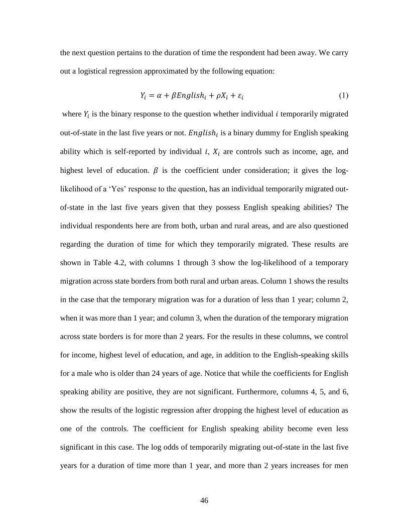
the next question pertains to the duration of time the respondent had been away. We carry

out a logistical regression approximated by the following equation:

𝑌𝑖 = 𝛼 + 𝛽𝐸𝑛𝑔𝑙𝑖𝑠ℎ𝑖 + 𝜌𝑋𝑖 + 𝜀𝑖 (1)

where 𝑌𝑖 is the binary response to the question whether individual 𝑖 temporarily migrated

out-of-state in the last five years or not. 𝐸𝑛𝑔𝑙𝑖𝑠ℎ𝑖 is a binary dummy for English speaking

ability which is self-reported by individual 𝑖, 𝑋𝑖 are controls such as income, age, and

highest level of education. 𝛽 is the coefficient under consideration; it gives the log-

likelihood of a ‘Yes’ response to the question, has an individual temporarily migrated out-

of-state in the last five years given that they possess English speaking abilities? The

individual respondents here are from both, urban and rural areas, and are also questioned

regarding the duration of time for which they temporarily migrated. These results are

shown in Table 4.2, with columns 1 through 3 show the log-likelihood of a temporary

migration across state borders from both rural and urban areas. Column 1 shows the results

in the case that the temporary migration was for a duration of less than 1 year; column 2,

when it was more than 1 year; and column 3, when the duration of the temporary migration

across state borders is for more than 2 years. For the results in these columns, we control

for income, highest level of education, and age, in addition to the English-speaking skills

for a male who is older than 24 years of age. Notice that while the coefficients for English

speaking ability are positive, they are not significant. Furthermore, columns 4, 5, and 6,

show the results of the logistic regression after dropping the highest level of education as

one of the controls. The coefficient for English speaking ability become even less

significant in this case. The log odds of temporarily migrating out-of-state in the last five

years for a duration of time more than 1 year, and more than 2 years increases for men

47

above 24 years of age who can speak English. Coefficients for other explanatory variables

are insignificant. We can therefore conclude that while English speaking ability increases

the likelihood that an individual would temporarily migrate across state borders, it however

is not significant, and even less significant if one does not take into consideration the

highest level of education for the individuals. In addition to the logistic regression, we also

perform a Poisson regression for equation (1) and obtain the incident rate ratios, which are

contained in Table 4.3. The results show that the incident rate for English speakers is 1.1

times the incident rate for non-English speakers when it comes to migrating temporarily

across state borders, which is not significantly large.

We now consider Hindi language as a factor in movement across state borders. As

has been mentioned above, Hindi is the mother tongue of at least ten out of the 29 states,

and is a second language in some other states. That said, there are many states where Hindi

is neither the state-language, nor is it spoken or understood in any significant measure. We

therefore use as control, a binary variable for Hindi not as the official state language. The

binary variable takes the value 1, if Hindi is not the official state language, and zero

otherwise. A logistic regression is performed on the following equation (2):

𝑌𝑖 = 𝛼 + 𝛽1𝐸𝑛𝑔𝑙𝑖𝑠ℎ𝑖 + 𝛽2𝐻𝑖𝑛𝑑𝑖_𝑜𝑓𝑓𝑖𝑐𝑖𝑎𝑙𝑖 + 𝜌𝑋𝑖 + 𝜀𝑖 (2)

where 𝑌𝑖 is the binary response to the question whether individual 𝑖 temporarily migrated

out-of-state in the last five years or not. 𝐸𝑛𝑔𝑙𝑖𝑠ℎ𝑖 is a dummy for self-reported English

speaking ability as was the case with equation (1), 𝐻𝑖𝑛𝑑𝑖_𝑜𝑓𝑓𝑖𝑐𝑖𝑎𝑙𝑖 is the dummy for

whether the official language of a state 𝑖 is not Hindi. 𝑋𝑖 are controls such as income, age,

residence (urban or rural) and highest level of education. Results of the logistic regression

for equation (2) are presented in Table 4.4, where one can notice that Hindi not being the

48

official language in a state is significant hurdle to the movement across state borders. The

coefficient for ‘Hindi not official state language’, is negative and highly significant for all

durations of temporary migrations as shown in columns (1), (2), and (3), of Table 4.4.

Moreover, upon controlling for Hindi as the official language at the state level, English

speaking ability is positive and significant at 5% level. The size of the coefficient rises

slightly with the duration, even as the coefficient for English speaking ability is

insignificant when the duration of temporary migration across state borders is less than 1

year. The result from Table 4.4 shows that for states where the official language (mother

tongue) is not Hindi, most migrants would come from within the state, and not outside the

state. This inference is corroborated by the 2011 census data for migrants across various

cities in India. Table 4.5 contains this information extracted from 2011 census survey of

India. This table does not include Delhi among the cities listed; this is because Delhi is

akin to a ‘city-state’, similar to the District of Columbia in the United States, where by its

very nature, most migrants come from outside the city. It is nonetheless, quite telling, that

even IT-Hubs like, Bangalore and Hyderabad have 56% and 81% of their long-term

immigrant residents respectively, from within the state instead of them belonging from

other parts of the country.

6. Human Capital and Migration in India

Chauvin et al. (2017) find substantial wage premium associated with Indian cities

as compared to cities in the US, Brazil, and China. They are however, unable to explain

why this might be the case. They speculate that this high wage premium in Indian cities

might point to some unobserved human capital. In this section we will attempt to explore

any relationship between human capital and urbanization in the Indian context. Such a

49

connection, we expect, will shed some light on the high wage premiums associated with

cities in India. The relationship between migrating to a city and human capital might be

approximated by the following equation (3):

𝑌𝑖 = 𝛼 + 𝛽1𝐸𝑛𝑔𝑙𝑖𝑠ℎ𝑖 + 𝛽2𝐻𝑖𝑔ℎ𝑒𝑠𝑡 𝑙𝑒𝑣𝑒𝑙 𝑜𝑓 𝑒𝑑𝑢𝑐𝑎𝑡𝑖𝑜𝑛𝑖 + 𝜌𝑋𝑖 + 𝜀𝑖 (3)

where 𝑌𝑖 is the binary choice variable of whether an individual 𝑖 migrated on a temporary

basis to an urban or a rural destination in the last five years. 𝐸𝑛𝑔𝑙𝑖𝑠ℎ𝑖 is a dummy for

English speaking ability of an individual 𝑖 which is self-reported.,

𝐻𝑖𝑔ℎ𝑒𝑠𝑡 𝑙𝑒𝑣𝑒𝑙 𝑜𝑓 𝑒𝑑𝑢𝑐𝑎𝑡𝑖𝑜𝑛𝑖 for an individual 𝑖 is a measure of human capital that the

individual possesses. 𝑋𝑖 are controls such as income, age, residence (urban or rural). The

observations are restricted to males older than 24 years of age. Table 4.6 contains the results

of the logistic regression performed on equation (3). The results show that the coefficient

for 𝐻𝑖𝑔ℎ𝑒𝑠𝑡 𝑙𝑒𝑣𝑒𝑙 𝑜𝑓 𝑒𝑑𝑢𝑐𝑎𝑡𝑖𝑜𝑛𝑖 are strongly significant and positive. More educated

men who are more than 24 years old, are more likely to migrate temporarily to an urban

area for a duration of up to 1 year, and more than 1 year. Coefficient for the duration in

excess of 2 years is positive, but less significant. This might be due to small number of

observations. Furthermore, for those who reside in rural areas as well, better educated men

aged 24 years and above, are more likely to migrate temporarily to an urban area. As more

educated people move to the cities, this perhaps explains high wage premiums in Indian

cities. That said, cities in other parts of the world also attract more educated individuals

with specialist jobs opportunities. In the Indian context then, either more educated

individuals are a lot more scarce compared to other countries, or that there is a much greater

concentration of jobs requiring higher education in Indian cities compared to cities in other

countries. This requires further exploration, which is beyond this scope of this study. It is

50

quite possible that both scenarios coexist. It is well known that for the most part of the last

70 years since India’s independence, the country has suffered from shoddy infrastructure

across the country of the most basic kind. This has over the years meant that many of the

jobs that do require a workforce that is well endowed in human capital, are concentrated in

a handful of cities where the infrastructure is relatively much better developed.

Furthermore, as has been shown in the previous section, mobility across state borders is

hindered by linguistic diversity. This would imply that well-educated individuals may not

migrate to different parts of the country in their job seeking efforts, and hence, there might

a scarcity of well-educated people in Indian cities, causing the wage for such individuals

to attract a significant premium.

7. Conclusion

We have tried to address some of the issues that had been raised by Chauvin et al.

(2016). In doing so, we have tried to consider linguistic diversity in India, and explore

aspects of human capital and its relationship with migration. We show that linguistic

diversity does affect the mobility of individuals across state borders in India. Specifically,

if Hindi is not the official language of a state, the individual residents find it quite a barrier

to overcome to be able to go to different parts of the country. Controlling for Hindi not

being a state’s official language, we find that the self-reported English speaking ability

positively affects mobility across state borders.

We also show that cities in India do attract the more highly educated individuals

including those from rural areas. This may be due to urban-rural disparity in terms of the

types of jobs available in each of these places. Certain jobs might almost be monopolized

in the urban areas, e.g. good university/academic jobs, which are almost exclusively in

51

urban settings in India; and same is the case with hospitals, manufacturing, and IT related

industry. Cities in India have had the advantage over rural areas in terms of better basic

infrastructure, which has allowed for almost all of well-paying jobs that require higher

education, to be almost exclusively be based out of cities. Not to mention that if even the

well-educated individuals find it difficult to be mobile across state borders, then that may

create a shortage of well-educated workers, pushing the wages up, and therefore we find

substantial wage premium associated with Indian cities as compared cities in other parts of

the world. Finally, we would also like to mention some shortcomings of our study that are

borne out of the IHDS-II dataset. The dataset considers and reports on only those

individuals who migrated temporarily, and returned back to their own homes in the last

five years from the date of the interview. A more elaborate study would be able to include

migrants to Indian cities who have decided to stay and not return to their native towns and

villages. Currently the IHDS-II dataset does not allow for such an exploration. Another

issue with the dataset is that the number of observation reduces drastically as one tries to

include variables such as the self-reporting English speaking ability. Small numbers of

observations might lead to untrustworthy findings.

52

Table 4.1 Temporary Migrant in the last five years

This table presents a summary of the number of individual respondents to the IHDS-II

survey who had migrated out of their place of residence temporarily in the last five years,

and have since returned.

Frequency Percentage Cumulative

No 201,280 98.39 98.39

Yes 3,289 1.61 100.00

Total 204, 569 100.00

53

Table 4.2: Temporary Out-of-State Migration

This table shows the impact of various variables on the choice and the likelihood of an

individual to migrate outside their own state.

(1) (2) (3) (4) (5) (6)

Duration

less than

1yr.

Duration

more than

1yr.

Duration

more than

2yrs.

Duration

less than

1yr.

Duration

more than

1yr.

Duration

more than

2yrs. English 0.205 0.504* 0.736* 0.175 0.358 0.021

(0.133) (0.302) (0.382) (0.120) (0.260) (0.411)

Highest level

of education -0.006

(0.011) -0.025

(0.026) -0.052

(0.035)

Log of income -0.078* -0.063 0.127 -0.084* -0.083 0.100

(0.047) (0.110) (0.153) (0.046) (0.108) (0.161)

Age -0.012** 0.005 0.008 -0.011** 0.007 0.015

(0.005) (0.011) (0.015) (0.004) (0.011) (0.019)

constant 1.470*** 1.052 -1.073 1.486*** 1.049 -1.299

(0.520) (1.280) (1.790) (0.519) (1.285) (2.010)

Obs. 2102 403 226 2102 403 148

Note: observations include males older than 24 yrs. of age, from both, rural and urban areas.

Standard errors are in parenthesis.

Asterisks denote significance levels (* = 0.1, ** = 0.05, *** = 0.01)

54

Table 4.3: Temporary Out-of-State Migration Poisson Regression

This table shows results for a Poisson regression where each column reports the incident rate ratio

(IRR).

Note: observations include males older than 24 years of age from both, rural and urban areas.

Standard errors in parenthesis

Asterisks denote significance levels (* = 0.1, ** = 0.05, *** = 0.01)

(1) (2) (3)

Duration

less than 1yr. Duration

more than 1yr. Duration

more than 2yrs. (IRR) (IRR) (IRR)

English 1.093 1.204* 1.335*

(0.095) (0.216) (0.313)

Highest level of education 0.997 0.990 0.979 (0.007) (0.016) (0.022)

Log of income 0.966* 0.977* 1.052

(0.030) (0.065) (0.100)

Age 0.995** 1.002 1.003

(0.003) (0.006) (0.009)

constant 0.968*** 0.762 0.330

(0.330) (0.590) (0.371)

Obs. 2102 403 226

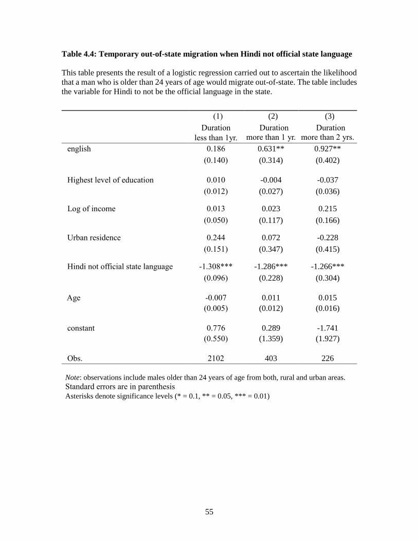
55

Table 4.4: Temporary out-of-state migration when Hindi not official state language

This table presents the result of a logistic regression carried out to ascertain the likelihood

that a man who is older than 24 years of age would migrate out-of-state. The table includes

the variable for Hindi to not be the official language in the state.

(1) (2) (3)

Duration

less than 1yr.

Duration

more than 1 yr.

Duration

more than 2 yrs.

english 0.186 0.631** 0.927**

(0.140) (0.314) (0.402)

Highest level of education 0.010 -0.004 -0.037

(0.012) (0.027) (0.036)

Log of income 0.013 0.023 0.215

(0.050) (0.117) (0.166)

Urban residence 0.244 0.072 -0.228

(0.151) (0.347) (0.415)

Hindi not official state language -1.308*** -1.286*** -1.266***

(0.096) (0.228) (0.304)

Age -0.007 0.011 0.015

(0.005) (0.012) (0.016)

constant 0.776 0.289 -1.741

(0.550) (1.359) (1.927)

Obs. 2102 403 226

Note: observations include males older than 24 years of age from both, rural and urban areas. Standard errors are in parenthesis

Asterisks denote significance levels (* = 0.1, ** = 0.05, *** = 0.01)

56

Table 4.5 Share of Total Migrants from within India for selected large cities.

This table presents a snapshot of the share of total immigrants, both recent, and long-term,

who migrate to a large city from either within the same state, or from outside the state. The

table below also highlights the different official languages in different states, alongside the

second languages.

Source: Census of India 2001, Table D-3

Notes: Delhi is not included in the list because it is “city state”, and all immigrants into

Delhi are by definition from outside Delhi and the distinction as made in the last two

columns, cannot be made for Delhi. The more recent, 2011 census could not be used as this

specific data has not yet been made publicly available.

Share of Total (Urban and Rural)

Migrants from within India

City State

Official State

Language

Second

Language Duration of

Residence From within

the State From outside

the State

Mumbai

(Bombay)

Maharashtra Marathi 1 - 4 years 35% 65%

Hindi 10 yrs. and more 43.70% 56.30%

Kolkata

(Calcutta) West Bengal Bengali 1 - 4 years 63.40% 36.60%

Hindi 10 yrs. and more 52.70% 47.30%

Chennai

(Madras)

Tamil Nadu Tamil 1 - 4 years 76.90% 23.10%

Telugu 10 yrs. and more 78.80% 21.20%

Bengaluru

(Bangalore) Karnataka Kannada 1 - 4 years 51.50% 48.50%

Tamil 10 yrs. and more 56.10% 43.90%

Hyderabad Andhra Pradesh Telugu 1 - 4 years 81.50% 18.50%

Urdu 10 yrs. and more 81.50% 18.50%

Ahmedabad Gujarat Gujarati 1 - 4 years 68.50% 31.50%

Hindi 10 yrs. and more 69.20% 30.80%

Pune Maharashtra Marathi 1 - 4 years 63.60% 36.40%

Hindi 10 yrs. and more 75.40% 24.60%

Surat Gujarat Gujarati 1 - 4 years 49.40% 50.60%

Hindi 10 yrs. and more 54.50% 45.50%

Jaipur Rajasthan Hindi 1 - 4 years 63.00% 37%

Urdu 10 yrs. and more 69.80% 30.20%

57

Table 4.6: Temporary Migration to Urban Area

This table shows the influence of a variety of factors on an individual’s choice to

temporarily migrate to an urban area in India.

(1) (2) (3)

Duration

less than 1yr.

Duration

more than 1 yr.

Duration

more than 2 yrs.

english -0.046 0.251 0.130

(0.150) (0.340) (0.438)

Highest level of education 0.070*** 0.088*** 0.056

(0.012) (0.029) (0.038)

Log of income -0.093* -0.178 0.070

(0.052) (0.125) (0.173)

Rural residence -0.624*** -0.657 -0.375

(0.173) (0.402) (0.472)

Hindi not official state language -0.244** -0.378 0.089

(0.098) (0.232) (0.306)

Age -0.015*** 0.001 -0.013

(0.005) (0.012) (0.016)

constant 2.519*** 2.842* 0.458

(0.614) (1.553) (2.147)

Obs. 2101 403 226

Note: observations include males older than 24 years of age from both, rural and urban areas. Standard errors are in parenthesis

Asterisks denote significance levels (* = 0.1, ** = 0.05, *** = 0.01)

58

REFERENCES

Azam, M., Chin, A., Prakash, N. (2010). The returns to English-language skills in India.

IZA Discussion Papers, No. 4802

Baye, M., Kovenock, D., and De Vries, C. (1993). Rigging the Lobbying Process: An

Application of the All-Pay Auction. American Economic Review ,83, 289 – 294.

Baye, M., Kovenock, D., and De Vries, C. (1996). The all-pay auction with

complete-information. Economic Theory, 8, 291 – 305.

Chakraborty, T. and Bakshi, S. K. (2016) English language premium: Evidence from a

policy experiment in India. Economics of Education Review, 50, 1 – 16.

Chandrashekhar, S. and Sharma, A. (2015). Urbanization and spatial patterns of internal

migration in India. Spatial Demography, 3(2), 63 – 89.

Chauvin, J. P., et. al. (2017). What is different about urbanization in rich and poor

countries? Cities in Brazil, China, India and the United States. Journal of Urban

Economics, 98, 17 – 49.

Che, Y. and Gale I. (1998). Caps on Political Lobbying. American Economic Review, 88,

643 – 51.

Che, Y. and Gale I. (2006). Caps on Political Lobbying: Reply. American Economic

Review, 96, 1355 – 60.

Chen, N. (2004). Intra-national versus international trade in the European Union: why do

national borders matter? Journal of International Economics, 63(1), 93 – 118.

Clingingsmith, D. (2014). Industrialization and Bilingualism in India. Journal of Human

Resources, 49, 73 – 109.

Desai, S. and Reeve V. (2016). India Human Development Survey-II (IHDS-II), 2011-12.

ICPSR36151-v5. Ann Arbor, MI: Inter-university Consortium for Political and

Social Research

Gavious, A., Moldovanu, B., and Sela, A. (2002). Bid Costs and Endogenous Caps. RAND

Journal of Economics, 33, 709 – 722.

Hillman A. and Riley, J. (1989). Politically Contestable Rents and Transfers. Economics

and Politics, 1, 17 – 39.

59

Hohenthal, A. (2003) English in India: Loyalty and Attitudes. Language in India, 3.

Kaplan, T. and Wettstein, D. (2006). Caps on Political Lobbying: Comment. American

Economic Review, 96, 1351 – 54.

Kone, Z. L., et. al. (2018) Internal borders and migration in India, Journal of Economic

Geography, 18(4), 729 – 759

Lusome, R. and R. Bhagat (2006). Trends and patterns of internal migration in india, 1971

– 2001. In Paper presented at the Annual Conference of Indian Association for the

Study of Population (IASP) during, Volume 7, 9.

Mayda, A. M. (2010). International migration: A panel data analysis of the determinants

of bilateral flows. Journal of Population Economics. 23(4), 1249–1274.

Molloy, R., C. L. Smith, and A. Wozniak (2011). Internal migration in the united states.

The Journal of Economic Perspectives. 25 (3), 173–196.

Munshi K., Rosenzweig M. (2006). Traditional institutions meet the modern world: Caste,

gender and schooling choice in a globalizing economy. American Economic

Review, 96(4), 1225 – 1252.

Munshi K., Rosenzweig M. (2016). Networks and misallocation: Insurance, migration, and

the rural-urban wage gap. The American Economic Review. 106(1), 46 – 98.

Olofsson, P. and Andersson M. (2012). Probability, Statistics, and Stochastic Processes.

John Wiley & Sons, Inc.

Olszewski, W., Seigel, R. (2019). Bid Caps in Large Contests. Games and Economic

Behavior, In press.

Pastine, I. and Pastine, T. (2013). Soft Money and Campaign Finance Reform.

International Economic Review, 54, 1118 – 1131.

Poncet, S. (2006). Provincial migration dynamics in china: Borders, costs, and economic

motivations. Regional Science and Urban Economics. 36(3), 385 – 398.

Roy, J. (2004). Can Changing Academic Standards Affect Educational Outcomes?

Evidence from a Policy Experiment in India. Georgetown University unpublished

paper.

Shastry, G. K. (2012). Human capital response to globalization: Education and information

technology in India. Journal of Human Resources, 47, 287 – 330.

Srivastava, R. and S. Sasikumar (2003). An overview of migration in India, its impacts and

key issues. In Regional Conference on Migration, Development and Pro-Poor

Policy Choices in Asia. 22 – 24.

Siegel, R. (2009). All-Pay Contests. Econometrica, 77, 71 – 92.

60

Siegel, R. (2010). Asymmetric Contests with Conditional Investments. American

Economic Review, 100, 2230 – 2260.

Siegel, R. (2014). Asymmetric Contests with Head Starts and Nonmonotonic Costs.

American Economic Journal: Microeconomics, 6, 59 – 105.

Szech, N. (2015). The all-pay auction with complete-information. Games and Economic

Behavior, 92, 138.149.

Tumbe, C. (2016). Urbanization, Demographic Transition and the Growth of Cities in

India, 1870-2020. Working Paper. International Growth Centre C-35205-INC-1.

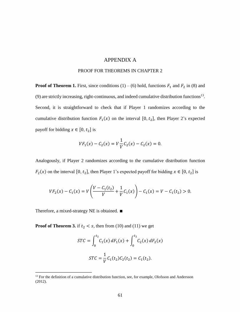
61

APPENDIX A

PROOF FOR THEOREMS IN CHAPTER 2

Proof of Theorem 1. First, since conditions (1) – (6) hold, functions 𝐹1 and 𝐹2 in (8) and

(9) are strictly increasing, right-continuous, and indeed cumulative distribution functions13.

Second, it is straightforward to check that if Player 1 randomizes according to the

cumulative distribution function 𝐹1(𝑥) on the interval [0, 𝑡2], then Player 2’s expected

payoff for bidding 𝑥 ∈ [0, 𝑡2] is

𝑉𝐹1(𝑥) − 𝐶2(𝑥) = 𝑉1

𝑉𝐶2(𝑥) − 𝐶2(𝑥) = 0.

Analogously, if Player 2 randomizes according to the cumulative distribution function

𝐹2(𝑥) on the interval [0, 𝑡2], then Player 1’s expected payoff for bidding 𝑥 ∈ [0, 𝑡2] is

𝑉𝐹2(𝑥) − 𝐶1(𝑥) = 𝑉 (𝑉 − 𝐶1(𝑡2)

𝑉+1

𝑉𝐶1(𝑥)) − 𝐶1(𝑥) = 𝑉 − 𝐶1(𝑡2) > 0.

Therefore, a mixed-strategy NE is obtained. ∎

Proof of Theorem 3. if 𝑡2 < 𝑠, then from (10) and (11) we get

𝑆𝑇𝐶 = ∫ 𝐶1(𝑥)𝑡2

0

𝑑𝐹1(𝑥) + ∫ 𝐶2(𝑥)𝑡2

0

𝑑𝐹2(𝑥)

𝑆𝑇𝐶 =1

𝑉𝐶1(𝑡2)𝐶2(𝑡2) = 𝐶1(𝑡2).

13 For the definition of a cumulative distribution function, see, for example, Olofsson and Andersson

(2012).

62

Suppose that 𝑡2 ≥ 𝑠. Then,

𝑆𝑇𝐶 =1

𝑉∫ 𝐿1(𝑥)𝑠

0

𝑑𝐿2(𝑥) +1

𝑉∫ (𝐿1(𝑥)𝑡2

𝑠

+𝑚) 𝑑(𝐿2(𝑥) + 𝑚) +

1

𝑉∫ 𝐿2(𝑥)𝑠

0

𝑑𝐿1(𝑥) +1

𝑉∫ (𝐿2(𝑥)𝑡2

𝑠

+𝑚) 𝑑(𝐿1(𝑥) + 𝑚) ,

=1

𝑉𝐿2(𝑠)𝐿1(𝑠) +

1

𝑉∫ (𝐿1(𝑥)𝑡2

𝑠

+𝑚) 𝑑(𝐿2(𝑥) + 𝑚) +

1

𝑉((𝐿2(𝑡2) + 𝑚)(𝐿1(𝑡2) + 𝑚) − (𝐿2(𝑠) + 𝑚)(𝐿1(𝑠) + 𝑚))

−1

𝑉∫ (𝐿1(𝑥)𝑡2

𝑠

+𝑚) 𝑑(𝐿2(𝑥) +𝑚),

𝑆𝑇𝐶 = 𝐶1(𝑡2)−𝑚

𝑉(𝐿1(𝑠)+ 𝐿2(𝑠)+𝑚).

Analogously, for aggregate bids with soft caps,

𝑆𝐴𝐵 = ∫ 𝑥𝑡2

0

𝑑𝐹1(𝑥) + ∫ 𝑥𝑡2

0

𝑑𝐹2(𝑥)

𝑆𝐴𝐵 =1

𝑉(∫ 𝑥

𝑠

0

𝑑𝐿2(𝑥) + ∫ 𝑥𝑡2

𝑠

𝑑𝐿2(𝑥) + ∫ 𝑥𝑠

0

𝑑𝐿1(𝑥) + ∫ 𝑥𝑡2

𝑠

𝑑𝐿1(𝑥)) ,

=1

𝑉((𝑥(𝐿2(𝑥) + 𝐿1(𝑥)))|

0

𝑠

+ (𝑥(𝐿2(𝑥) + 𝐿1(𝑥)))|𝑠

𝑡2

− (∫ 𝐿1(𝑥)𝑠

0

𝑑𝑥 + ∫ 𝐿1(𝑥)𝑡2

𝑠

𝑑𝑥 + ∫ 𝐿2(𝑥)𝑠

0

𝑑𝑥 + ∫ 𝐿2(𝑥)𝑡2

0

𝑑𝑥)) ,

𝑆𝐴𝐵 =1

𝑉(𝑡2(𝐿1(𝑡2) + 𝐿2(𝑡2)) − (∫ 𝐿1(𝑥)𝑑𝑥

𝑡2

0

+∫ 𝐿2(𝑥)𝑑𝑥𝑡2

0

)).

∎

63

APPENDIX B

PROOF FOR THEOREMS IN CHAPTER 3

Proof of Theorem 1. Suppose that conditions (1) – (5) and (9) hold and each player bids

the rigid cap 𝑟. Then, player 𝑖 gets the following payoff

𝑢𝑖(𝑟, 𝑟) =𝑉

2− 𝐶𝑖(𝑟) ≥ 0

and cannot increase her payoff given the bid of her opponent. ∎

Proof of Theorem 2. First, since conditions (1) – (5), and (10) hold, functions 𝐻1 and 𝐻2

in (12) and (13) respectively, are strictly increasing and indeed cumulative distribution

functions.

Second, it is straightforward to check that if Player 1 randomizes according to the

cumulative distribution function 𝐹1(𝑥) on the interval [0, 𝑡], then Player 2’s expected

payoff for bidding 𝑥 ∈ [0, 𝑡] is

𝑉𝐻1(𝑥) − 𝐿2(𝑥) = 𝑉1

𝑉𝐿2(𝑥) − 𝐿2(𝑥) = 0.

Suppose that Player 2 bids 𝑥 = 𝑟. Then, her expected payoff is

𝑉𝐻1(𝑡) +1

2(1 − 𝐻1(𝑡))𝑉 − 𝐿2(𝑟) = 0,

where the first term is the expected benefit, if Player 1 bids in the interval [0, 𝑡], the second

term is the expected benefit, if Player 1 bids exactly the rigid cap, 𝑟, and the last term is

64

the cost of bidding. The expected payoff has to be the same as the expected payoff after

Player 2 bids on the interval [0, 𝑡].

We get

𝐻1(𝑡) =2

𝑉𝐿2(𝑟) − 1.

Since

𝐻1(𝑡) =1

𝑉𝐿2(𝑡),

We obtain

𝐿2(𝑡) = 2𝐿2(𝑟) − 𝑉,

or

𝑡 = 𝐿2−1(2𝐿2(𝑟) − 𝑉).

Analogously, if Player 2 randomizes according to the cumulative distribution function

𝐻2(𝑥) on the interval [0, 𝑡], then Player 1’s expected payoff for bidding 𝑥 ∈ [0, 𝑡] is

𝑉𝐻2(𝑥) − 𝐿1(𝑥) = 𝑉𝐻2(𝑡) − 𝐿1(𝑡).

Suppose that player 1 bids 𝑥 = 𝑟. Then, her expected payoff is

𝑉𝐻2(𝑡) +1

2(1 − 𝐻2(𝑡))𝑉 − 𝐿1(𝑟) = 𝑉𝐻2(𝑡) − 𝐿1(𝑡),

since she has to be indifferent among her bids.

Therefore,

65

1

2(1 − 𝐻2(𝑡))𝑉 = 𝐿1(𝑟) − 𝐿1(𝑡) (i)

and

1

2(1 + 𝐻2(𝑡))𝑉 − 𝑉𝐻2(𝑥) = 𝐿1(𝑟) − 𝐿1(𝑥). (ii)

summing (i) and (ii), we get

𝑉 − 𝑉𝐻2(𝑥) = 2𝐿1(𝑟) − 𝐿1(𝑥) − 𝐿1(𝑡),

or

𝐻2(𝑥) = 1 −1

𝑉(2𝐿1(𝑟) − 𝐿1(𝑥) − 𝐿1(𝑡)).

Therefore, a mixed-strategy NE is obtained. ∎

Proof of Theorem 3.

𝑅𝑇𝐶(𝑟) = ∫ 𝐿1(𝑥)𝑟

0

𝑑𝐻1(𝑥) + ∫ 𝐿2(𝑥)𝑟

0

𝑑𝐻2(𝑥)

= ∫ 𝐿1(𝑥)𝑡

0

𝑑𝐻1(𝑥) + 𝐿1(𝑟)𝐻1(𝑟) + ∫ 𝐿2(𝑥)𝑡

0

𝑑𝐻2(𝑥) + 𝐿2(𝑟)𝐻2(𝑟)

or

=1

𝑉∫ 𝐿1(𝑥)𝑡

0

𝑑𝐻2(𝑥) + 𝐿1(𝑟)(1 − 𝐻1(𝑡)) +

∫ 𝐿2(𝑥)𝑡

0

𝑑 (𝑉 − (2𝐿1(𝑟) − 𝐿1(𝑡))

𝑉+1

𝑉𝐿1(𝑥)) + 𝐿2(𝑟)(1 − 𝐻2(𝑡)),

66

=1

𝑉∫ 𝐿1(𝑥)𝑡

0

𝑑𝐿2(𝑥) + 𝐿1(𝑟)(1 − 𝐻1(𝑡)) +1

𝑉∫ 𝐿2(𝑥)𝑡

0

𝑑𝐿1(𝑥) + 𝐿2(𝑟)(1 − 𝐻2(𝑡)),

=1

𝑉𝐿1(𝑡)𝐿2(𝑡) + 𝐿1(𝑟)(1 − 𝐿1(𝑡)) + 𝐿2(𝑟)(1 − 𝐻2(𝑡)),

=1

𝑉𝐿1(𝑡)𝐿2(𝑡) + 𝐿1(𝑟) (1 −

1

𝑉𝐿2(𝑡))

+ 𝐿2(𝑟)(1 − (𝑉 − (2𝐿1(𝑟) − 𝐿1(𝑡))

𝑉+1

𝑉𝐿1(𝑡))) ,

=1

𝑉𝐿1(𝑡)𝐿2(𝑡) + 𝐿1(𝑟) (1 −

1

𝑉𝐿2(𝑡)) + 𝐿2(𝑟)(1 − (

𝑉 − 2(𝐿1(𝑟) − 𝐿1(𝑡))

𝑉)) ,

=1

𝑉𝐿1(𝑡)𝐿2(𝑡) + 𝐿1(𝑟) (1 −

1

𝑉𝐿2(𝑡)) + 𝐿2(𝑟) (

2(𝐿1(𝑟) − 𝐿1(𝑡))

𝑉) ,

= 𝐿1(𝑟) +1

𝑉(𝐿1(𝑡)𝐿2(𝑡) − 𝐿1(𝑟)𝐿2(𝑡) + 2𝐿2(𝑟)(𝐿1(𝑟) − 𝐿1(𝑡))) ,

since

𝑡 = 𝐿2−1(2𝐿2(𝑟) − 𝑉),

we get

𝑅𝑇𝐶(𝑟) = 𝐿1(𝑟)

+1

𝑉(𝐿1(𝑡)(2𝐿2(𝑟) − 𝑉) − 𝐿1(𝑟)(2𝐿2(𝑟) − 𝑉)

+ 2𝐿2(𝑟)(𝐿1(𝑟) − 𝐿1(𝑡))) ,

67

= 𝐿1(𝑟) +1

𝑉(2𝐿1(𝑡)𝐿2(𝑟) − 𝑉𝐿1(𝑡) − 2𝐿1(𝑟)𝐿2(𝑟) + 𝑉𝐿1(𝑟) + 2𝐿1(𝑟)𝐿2(𝑟)

− 2𝐿1(𝑡)𝐿2(𝑟)),

𝑅𝑇𝐶(𝑟) = 2𝐿1(𝑟) − 𝐿1(𝑡).

Analogously,

𝑅𝐴𝐵(𝑟) = ∫ 𝑥𝑟

0

𝑑𝐻1(𝑥) + ∫ 𝑥𝑟

0

𝑑𝐻2(𝑥)

= ∫ 𝑥𝑡

0

𝑑𝐻1(𝑥) + 𝑟𝐻1(𝑟) + ∫ 𝑥𝑡

0

𝑑𝐻2(𝑥) + 𝑟𝐻1(𝑟)

=1

𝑉∫ 𝑥𝑡

0

𝑑𝐿2(𝑥) + 𝑟(1 − 𝐻1(𝑡)) +1

𝑉∫ 𝑥𝑡

0

𝑑𝐿1(𝑥) + 𝑟(1 − 𝐻2(𝑡))

𝑅𝐴𝐵(𝑟) =1

𝑉(𝑡(𝐿1(𝑡) + 𝐿2(𝑡)) − ∫ (𝐿1(𝑡) + 𝐿2(𝑡))𝑑𝑥

𝑡

0

) + 𝑟(2 − 𝐻1(𝑡) − 𝐻2(𝑡)).

∎