Embed Size (px)
Citation preview

Essays in Labour Economics and
Entrepreneurship
Von der Wirtschaftswissenschaftlichen Fakultat der
Gottfried Wilhelm Leibniz Universitat Hannover
zur Erlangung des akademischen Grades
Doktorin der Wirtschaftswissenschaften
- Doctor rerum politicarum -
genehmigte Dissertation
von
MSc Helke Seitz
geboren am 30.07.1985 in Neustadt an der Weinstraße
2019

Referentin: Apl. Prof. Dr. Susan Steiner
Koreferent: Prof. Dr. Lukas Menkhoff
Tag der Promotion: 30.01.2019

Abstract
This dissertation is concerned with research questions in the fields of labour eco-
nomics and entrepreneurship. Chapter 1 introduces the four different research areas
of this thesis and provides an overview of the subsequent chapters.
Chapter 2 contributes to the understanding of the participation in on-the-job
training from a behavioural perspective. This is done by incorporating individual’s
subjective beliefs about the return to training. These beliefs depend on their locus
of control, a psychological concept about beliefs regarding an individual’s control
over the outcome of events in their life. Our empirical results suggest that having an
internal locus of control is associated with higher participation in general but not in
specific training. Specifically, general training is associated with greater expectations
of future wage growth for those with an internal locus of control. There is no evidence
of any link between locus of control and wage expectations or post-training wages
in case of specific training.
Chapter 3 evaluates the relationship between intergenerational co-residence and
female labour force participation in Kyrgyzstan. The direction of the effect is not
clear ex-ante. While elderly caretaking responsibilities might lead to lower labour
force participation, child care support offered by grandparents might lead to the
opposite effect. We find that co-residence has no effect on female labour force par-
ticipation and the number of working hours. While other studies find positive im-
pacts of co-residence on female labour force participation, we seek to analyze the
channels that might link co-residence and female labour force participation. We find
that intergenerational co-residence leads to around half an hour more spent per day
on elder care, on average. We find that this is at the expense of the women’s leisure
time.
Chapter 4 analyses constraints to investments of micro and small enterprises. I
find that in the overall estimation sample, savings and managerial constraints are as-
sociated with lower investments. Further, the paper identifies several subgroups that
are subject to certain constraints. These results reflect that savings and managerial
constraints are non-negligible factors for firm investments. The subsample analysis
provides an attempt to identify firms with similar constraints prior to treatment
assignment, which is important to correctly match client characteristics with the
type of training that will be useful for them.

Chapter 5 evaluates two different financial education trainings. The first teaches
simple rules of financial decision making (rule-of-thumb training) and the second
training includes, in addition to the rule-of-thumb training, an add-on where en-
trepreneurs receive individual information (personalized training) about the finan-
cial situation of their business. Our estimates show that both trainings are generally
effective. Evaluating the effect on each outcome family shows that the effect of
personalized training on savings is strongest, which is 0.279 SD units and highly
statistically significant.
Keywords: on-the-job training, intergenerational coresidence, constraints, microen-
terprises, financial education
ii

Contents
List of Figures vii
List of Tables viii
Abbreviations xii
1 Introduction 1
1.1 Research Area . . . . . . . . . . . . . . . . . . . . . . . . . . . . . . . 1
1.2 Motivation . . . . . . . . . . . . . . . . . . . . . . . . . . . . . . . . . 1
1.2.1 Essays in Labour Economics . . . . . . . . . . . . . . . . . . . 1
1.2.2 Essays in Entrepreneurship . . . . . . . . . . . . . . . . . . . . 3
1.3 Dissertation Outline . . . . . . . . . . . . . . . . . . . . . . . . . . . 4
2 Locus of Control and Investment in Training 9
2.1 Introduction . . . . . . . . . . . . . . . . . . . . . . . . . . . . . . . . 10
2.2 Theoretical Framework . . . . . . . . . . . . . . . . . . . . . . . . . . 13
2.2.1 Modeling the Training Investment Decision . . . . . . . . . . . 13
2.2.2 The Role of Locus of Control in the Investment Decision . . . 15
2.2.3 Model Extensions . . . . . . . . . . . . . . . . . . . . . . . . . 18
2.3 Data . . . . . . . . . . . . . . . . . . . . . . . . . . . . . . . . . . . . 22
iii

2.3.1 Estimation Sample . . . . . . . . . . . . . . . . . . . . . . . . 22
2.3.2 Training Measures . . . . . . . . . . . . . . . . . . . . . . . . 24
2.3.3 Locus of Control . . . . . . . . . . . . . . . . . . . . . . . . . 26
2.3.4 Wage Expectations, Realized Wages and Control Variables . . 28
2.4 Results . . . . . . . . . . . . . . . . . . . . . . . . . . . . . . . . . . . 30
2.4.1 Estimation Strategy . . . . . . . . . . . . . . . . . . . . . . . 30
2.4.2 Participation in Training . . . . . . . . . . . . . . . . . . . . . 31
2.4.3 Wage Expectations and Realized Wages . . . . . . . . . . . . 33
2.4.4 Robustness Analysis . . . . . . . . . . . . . . . . . . . . . . . 37
2.5 Conclusions . . . . . . . . . . . . . . . . . . . . . . . . . . . . . . . . 40
3 Patrilocal Residence and Female Labour Supply: Evidence from
Kyrgyzstan 43
3.1 Introduction . . . . . . . . . . . . . . . . . . . . . . . . . . . . . . . . 44
3.2 Background: Female Labour Supply in Kyrgyzstan . . . . . . . . . . 48
3.3 Data . . . . . . . . . . . . . . . . . . . . . . . . . . . . . . . . . . . . 50
3.3.1 Outcome Variables . . . . . . . . . . . . . . . . . . . . . . . . 51
3.3.2 Co-residence and Youngest Son . . . . . . . . . . . . . . . . . 53
3.3.3 Other Covariates . . . . . . . . . . . . . . . . . . . . . . . . . 53
3.4 Empirical Strategy and Results . . . . . . . . . . . . . . . . . . . . . 55
3.4.1 Discussion of Instrument and Identifying Assumptions . . . . 55
3.4.2 Estimation Results . . . . . . . . . . . . . . . . . . . . . . . . 59
3.4.3 Comparison of Estimated Effects with Other Countries . . . . 64
3.4.4 Channels . . . . . . . . . . . . . . . . . . . . . . . . . . . . . . 65
3.5 Conclusion . . . . . . . . . . . . . . . . . . . . . . . . . . . . . . . . . 69
iv

4 How do Investment Constraints and Business Characteristics Co-
incide? 71
4.1 Introduction . . . . . . . . . . . . . . . . . . . . . . . . . . . . . . . . 72
4.2 Literature Review . . . . . . . . . . . . . . . . . . . . . . . . . . . . . 74
4.3 Data . . . . . . . . . . . . . . . . . . . . . . . . . . . . . . . . . . . . 77
4.3.1 Estimation Sample . . . . . . . . . . . . . . . . . . . . . . . . 77
4.3.2 Outcome Variable: Investments . . . . . . . . . . . . . . . . . 78
4.3.3 Measurement of Constraints . . . . . . . . . . . . . . . . . . . 81
4.3.4 Generating Indices for each Constraint . . . . . . . . . . . . . 85
4.3.5 Other Covariates . . . . . . . . . . . . . . . . . . . . . . . . . 87
4.4 Empirical Analysis . . . . . . . . . . . . . . . . . . . . . . . . . . . . 89
4.4.1 Relation of Constraints on Investment . . . . . . . . . . . . . 89
4.4.2 Coincidence of Constraints and Characteristics . . . . . . . . . 91
4.4.3 Robustness Checks . . . . . . . . . . . . . . . . . . . . . . . . 98
4.5 Conclusion . . . . . . . . . . . . . . . . . . . . . . . . . . . . . . . . . 100
5 The Effects of a Personalized Finance Training on Small Enter-
prises 103
5.1 Introduction . . . . . . . . . . . . . . . . . . . . . . . . . . . . . . . . 104
5.2 Experimental Setting . . . . . . . . . . . . . . . . . . . . . . . . . . . 107
5.2.1 Experimental Design . . . . . . . . . . . . . . . . . . . . . . . 107
5.2.2 Empirical Strategy . . . . . . . . . . . . . . . . . . . . . . . . 109
5.3 Data . . . . . . . . . . . . . . . . . . . . . . . . . . . . . . . . . . . . 110
5.3.1 Sample . . . . . . . . . . . . . . . . . . . . . . . . . . . . . . . 110
5.3.2 Outcome Variables . . . . . . . . . . . . . . . . . . . . . . . . 111
5.3.3 Descriptive Statistics . . . . . . . . . . . . . . . . . . . . . . . 112
v

5.4 Results . . . . . . . . . . . . . . . . . . . . . . . . . . . . . . . . . . . 114
5.4.1 Main Treatment Effects . . . . . . . . . . . . . . . . . . . . . 114
5.4.2 Treatment Effects on Single Components . . . . . . . . . . . . 117
5.4.3 Analysis of Entrepreneurs with Savings Goals . . . . . . . . . 120
5.5 Conclusion . . . . . . . . . . . . . . . . . . . . . . . . . . . . . . . . . 123
Bibliography 125
Appendix A - Appendix for Chapter 2 143
Appendix B - Appendix for Chapter 3 159
Appendix C - Appendix for Chapter 4 173
Appendix D - Appendix for Chapter 5 177
Publications 179
vi

List of Figures
2.1 Description of the Data Structure . . . . . . . . . . . . . . . . . . . . 23
2.2 Predicted Wage Expectations by Locus of Control . . . . . . . . . . . 35
3.1 Co-Residence and Female Labour Force Participation Across Countries 45
3.2 Labour Force Participation in Kyrgyzstan, 1990-2016 . . . . . . . . . 49
4.1 Relevance of Items . . . . . . . . . . . . . . . . . . . . . . . . . . . . 86
4.2 Coincidence of Constraints and Characteristics . . . . . . . . . . . . . 97
A.1 Locus of Control: Factor Analysis and Distribution . . . . . . . . . . 157
vii

viii

List of Tables
2.1 Descriptives Course Characteristics . . . . . . . . . . . . . . . . . . . 25
2.2 Locus of Control Items 1999 and 2005 . . . . . . . . . . . . . . . . . . 27
2.3 Logit Estimation Results: Participation in Training (Marginal Ef-
fects) . . . . . . . . . . . . . . . . . . . . . . . . . . . . . . . . . . . 32
2.4 OLS Estimation Results: Wage Expectations . . . . . . . . . . . . . 34
2.5 OLS Estimation Results: Gross Log Hourly Wage (t+1) . . . . . . . 36
2.6 Robustness Analysis for Training Participation and Wage Expectations 39
3.1 Summary Statistics on Female Labour Supply, Instrument and Ex-
planatory Variables . . . . . . . . . . . . . . . . . . . . . . . . . . . . 52
3.2 Differences in Pre-Marriage Characteristics . . . . . . . . . . . . . . . 58
3.3 Estimation Results: Labour Force Participation . . . . . . . . . . . . 61
3.4 Estimation Results: Working Hours . . . . . . . . . . . . . . . . . . . 62
3.5 Channel Analysis I: Time Use Woman . . . . . . . . . . . . . . . . . 66
3.6 Channel Analysis II: Parents’ Financial Contributions and Gender
Preferences . . . . . . . . . . . . . . . . . . . . . . . . . . . . . . . . 68
4.1 Summary Statistics on Capital Stock and Investment . . . . . . . . . 80
4.2 Summary Statistics on Items measuring Constraints . . . . . . . . . . 83
4.3 Summary Statistics on Explanatory Variables . . . . . . . . . . . . . 88
ix

4.4 Random Effects Estimation Results: Log Investments . . . . . . . . . 90
4.5 Random Effects Estimation Results: Constraints . . . . . . . . . . . . 92
4.6 Heterogeneity Analysis: Socio-economic Characteristics . . . . . . . . 94
4.7 Heterogeneity Analysis: Business Characteristics . . . . . . . . . . . . 96
4.8 Random Effects Estimation Results: Log Investments . . . . . . . . . 99
5.1 Pre-Intervention Descriptive Statistics of Industry Sectors . . . . . . . 111
5.2 Pre-Intervention Descriptive Statistics . . . . . . . . . . . . . . . . . 113
5.3 Main Treatment Effects . . . . . . . . . . . . . . . . . . . . . . . . . 115
5.4 Investment . . . . . . . . . . . . . . . . . . . . . . . . . . . . . . . . . 118
5.5 Savings . . . . . . . . . . . . . . . . . . . . . . . . . . . . . . . . . . . 119
5.6 Profits . . . . . . . . . . . . . . . . . . . . . . . . . . . . . . . . . . . 119
5.7 Diversication . . . . . . . . . . . . . . . . . . . . . . . . . . . . . . . 120
5.8 Pre-Intervention Descriptive Statistics for Savings Goal Group . . . . 121
5.9 Main Treatment Effects for Entrepreneurs with Business related Sav-
ing Goal . . . . . . . . . . . . . . . . . . . . . . . . . . . . . . . . . . 122
A.1 Summary Statistics of Explanatory Variables . . . . . . . . . . . . . . 144
A.2 Logit Estimation Results: Participation in Training, General Train-
ing, Specific Training . . . . . . . . . . . . . . . . . . . . . . . . . . 146
A.3 OLS Estimation Results: Wage Expectations, controlling for General
and Specific Training . . . . . . . . . . . . . . . . . . . . . . . . . . 149
A.4 OLS Estimation Results: Gross Log Hourly Wage Income (t+1) . . . 153
B.1 List of Countries Used for Cross-Country Analysis . . . . . . . . . . 159
B.2 Non-Parametric Differences in Pre-Marriage Characteristics . . . . . . 162
B.3 Number Of Children Up To Age Five . . . . . . . . . . . . . . . . . . 163
B.4 Estimation Results: Number of Children up to Age 5 . . . . . . . . . 164
x

B.5 OLS Estimation Results: Labour Force Participation . . . . . . . . . 165
B.6 Two-stage Least-Squares Estimation Results: Co-Residence (First Stage)166
B.7 Two-stage Least-Squares Estimation Results: Labour Force Partici-
pation (Second Stage) . . . . . . . . . . . . . . . . . . . . . . . . . . 167
B.8 Tobit Estimation Results: Working Hours . . . . . . . . . . . . . . . 168
B.9 IV Tobit Estimation Results: Working Hours (Second Stage) . . . . . 169
B.10 Heterogeneity Analysis: Labour Force Participation . . . . . . . . . . 170
B.11 Heterogeneity Analysis: Working Hours . . . . . . . . . . . . . . . . 171
B.12 Summary Statistics of Variables used in Channel Analysis . . . . . . 172
B.13 Gender Attitude Items . . . . . . . . . . . . . . . . . . . . . . . . . . 172
C.1 Panel Attrition 2013-2017 . . . . . . . . . . . . . . . . . . . . . . . . 173
C.2 Number of Observations on Subitems: Credit Constraints . . . . . . 174
C.3 Managerial Constraint Items . . . . . . . . . . . . . . . . . . . . . . . 175
C.4 Random Effects Estimation Results: Log Investments . . . . . . . . . 176
D.1 Overview Training Program . . . . . . . . . . . . . . . . . . . . . . . 177
D.2 Statements on Separating Finances . . . . . . . . . . . . . . . . . . . 177
D.3 Effect on Aggregates . . . . . . . . . . . . . . . . . . . . . . . . . . . 178
D.4 Separating Finances . . . . . . . . . . . . . . . . . . . . . . . . . . . 178
xi

xii

Abbreviations
ANCOVA Analysis of covariance
ITT Intention-to-treat
IV Instrumental variable
LIK Life in Kyrgyzstan
LoC Locus of Control
MC Managerial constraint
MDE Minimum detectable effect
MSEs Micro and small enterprises
OLS Ordinary least-squares
PCA Principal component analysis
PT Personalized training
RCT Randomized controlled trial
ROSCA Rotating savings and credit association
RoT Rule-of-thumb training
SACCO Savings and credit cooperative
SC Savings constraint
SD Standard deviation
SOEP German Socio-Economic Panel
xiii


Chapter 1
Introduction
1.1 Research Area
This dissertation is concerned with research questions in the fields of labour eco-
nomics and entrepreneurship. While the first chapter elaborates on the relation-
ship between personality traits and on-the-job training, the second chapter eval-
uates the relationship between intergenerational co-residence and female labour
force participation in Kyrgyzstan. The last two chapters examine entrepreneur-
ship in developing countries and are concerned with the constraints of micro and
small enterprises and the evaluation of a training intervention.
1.2 Motivation
1.2.1 Essays in Labour Economics
On-the-job Training. The workplace is shaped by constant changes through
globalization, new technologies, and markets. Working in such an environment
requires workers to constantly adjust and develop their skills. Hence, lifelong
education, beyond formal school education is an integral part of work-life. Due to
the importance of continuous investments in human capital, both education and
training are promoted and on the political agenda of the European Commission
(2010), OECD (2014), and International Labour Organization (2010).
1

Chapter 1 2
The economic implications of work-related training are well documented.
Training participants are associated with higher job performance rating scores
(Bartel, 1995), higher likelihood of promotion (Bishop, 1990), and have higher
wages, as documented in a meta-analysis (Haelermans and Borghans, 2012). In
light of these positive effects, several characteristics that coincide with training
participation are identified. A higher formal education (Asplund, 2005), having
union-coverage (Booth et al., 2003), being male (Lynch, 1992), and being em-
ployed by a larger company (Georgellis and Lange, 2007) are all characteristics
associated with training participation. However, this does not explain why some
groups decide to participate in training and others do not. This is especially in-
teresting in light of high returns to training for groups with lower participation
probability (e.g. for the less educated; see Blundell et al. (1996); Fourage et al.
(2013)).
In light of the importance of lifelong learning and the economic effects of
work-related training, it is crucial to understand how individual behavior leads
to an underinvestment in training. This part of the dissertation contributes to the
ongoing literature on training participation by adopting a behavioral perspective.
This is done by incorporating individual’s subjective beliefs about the return to
training, which depends on their locus of control, a psychological concept about
beliefs regarding an individual’s control over the outcome of events in their life.
Female Labour Force Participation. The participation of women in the
labour market matters in several respect for the individual woman and her house-
hold. Empirical evidence links female labour force participation to increased bar-
gaining power in the household (Antman, 2014; Heath, 2014) and to beneficial
effects for her children in terms of higher preschool enrolment rates (O’Connor,
1988) and improved health (Thomas, 1997).
With these beneficial effects in mind, an observed decrease in women’s labour
market participation in Kyrgyzstan since the dissolution of the Soviet Union
in 1991 is worrisome. In 1990, around 83 percent of Kyrgyz women engaged in
the labour marked (Asian Development Bank, 2005). Since the independence
of Kyrgyzstan female labour force participation declined, leading to a widening
gender gap in the labour force participation rates. Against this background, it is
important to study the women’s behavior on the labour market and their decision

Chapter 1 3
to work in Kyrgyzstan.
Keeping the cultural context in mind, there are many factors that may in-
fluence women’s decisions to participate in the labour market. One factor are
high rates of migrants working abroad. Estimates for 2008-2013 suggest around
200,000 labour migrants, which amounts to 10 percent of the Kyrgyz population
(Yang, 2015). This might be relevant, as negative effects of labour migration on
female labour force participation are documented in the literature (Acosta, 2006;
Mendola and Carletto, 2012). Another potential influencing factor are intergener-
ational living arrangements. Hence, co-residence with parents(-in-law) may affect
female labour force participation. The direction of the effect is not clear ex-ante.
While elderly caretaking responsibilities might lead to lower labour force partici-
pation (Lilly et al., 2007), child care support offered by grandparents might lead
to the opposite effect (Posadas and Vidal-Fernandez, 2013).
This paper contributes to the understanding of female labour force partici-
pation by focusing on the latter determinant of intergenerational co-residence.
Kyrgyzstan is a patrilocal society, which means that women move in with their
husband’s parents or wider family upon marriage.
1.2.2 Essays in Entrepreneurship
Micro and small enterprises (MSEs) are an important part of the economy in
developing countries. They contribute to a large extend to employment and job
creation (Ayyagari, 2011). Many developing countries (e.g. Sub-Saharan Africa)
will experience a steep increase in the labour force caused by demographic shifts
in the next years. This employment challenge increases the need for a “job-rich
economic growth,” without it, unemployment rates will remain high and living
standards cannot improve (G-20 Finance Ministers and Central Bank Governors
Meeting, 2017). Hence, one key policy question that arises is if MSEs have the
potential to grow and to create jobs.
Typically, micro and small enterprises either do not grow much or they dis-
appear after a while. Around half of all small firms disappear within 6 years
(McKenzie and Woodruff, 2017). Given these facts, it is not surprising that the
distribution of firms is right skewed, with the majority of firms being small and
the distribution declining in firm size (Hsieh and Olken, 2014). There are several
potential reasons for the missing growth or development of MSEs. Above all are

Chapter 1 4
financing constraints. This comprises, on the one hand, of credit constraints due
to poorly functioning credit markets (Banerjee and Duflo, 2005). On the other
hand, insufficient accumulation of own financial resources prevents individuals
from making productive investments. The reasons for undersaving are manifold,
comprising lack of information (e.g. low levels of financial literacy), social con-
straints, and behavioral biases (Karlan et al., 2014). Besides financial reasons,
managerial skills are seen are crucial as they affect the production function of
firms (Bruhn et al., 2010).
This dissertation contributes to the ongoing literature on the development of
MSEs in two ways. First, it adds to the understanding on which of the aforemen-
tioned constraints are actually important for MSEs and for groups. Secondly, it
contributes to the literature that aims to improve business performance through
financial education interventions. Here, this dissertation probes whether personal-
ized feedback can increase the effectiveness of a training compared to a benchmark
training.
1.3 Dissertation Outline
This dissertation consists of four separate research papers. The papers in chapters
2, 3, and 5 are joint with co-authors. The work in Chapter 2 joint with Marco
Caliendo, Deborah Cobb-Clark, and Arne Uhlendorff is currently in a revise and
resubmit process at the Journal of Human Resources. Chapter 3 is based on a
paper with Andreas Landmann and Susan Steiner and is published in Demogra-
phy1. The paper in Chapter 5 is joint work with Antonia Grohmann and Lukas
Menkhoff. The field experiment in Chapter 5 was pre-registered at the AEA RCT
Registry on March 15, 2018.2 The following gives a brief outline of each chapter.
Chapter 2 incorporates individuals’ beliefs about wage expectations in the
decision to participate in on-the-job training. These beliefs depend on the worker’s
locus of control. Locus of control can be described as the “generalized attitude,
belief or expectancy regarding the nature of the causal relationship between one’s
own behavior and its consequences” (Rotter, 1966). Those with internal control
1Landmann, A., Seitz, H. & Steiner, S. Demography (2018). https://doi.org/10.1007/s13524-018-0724-1
2ID: AEARCTR-0002785; see: https://www.socialscienceregistry.org/trials/2785

Chapter 1 5
tend to believe that much of what happens in life is influenced by their own be-
havior, whereas those with external control are more likely to believe that life’s
outcomes are driven by external factors. We develop a theoretical two-period
model in which workers and firms participate in the decision to invest in training.
We incorporate locus of control in the model by assuming that workers with an
internal locus of control expect a higher wage return to their training investment.
Further, our model takes into account the transferability of skills as highlighted
by Becker (1962). The more general a training is, the more that the skills learned
are transferable, while specific skills are less transferable. The following testable
predictions are derived from the model: first, workers with an internal locus of
control are more likely to participate in training (unless it is perfectly specific).
Secondly, the more internal the higher are expectations about post-training wage
increases (this relationship is predicted to be stronger for general training). Third
and lastly, post-training wages are independent of their locus of control (as it is
assumed that locus of control is unrelated to productivity). Each of these predic-
tions is empirically validated using data from the German Socioeconomic Panel
(SOEP), a representative household panel survey. Our empirical results suggest
that having an internal locus of control is associated with higher participation
in general but not in specific training. Specifically, general training is associated
with greater expectations of future wage growth for those with an internal locus
of control. There is no evidence of any link between locus of control and wage
expectations or post-training wages in case of specific training.
Chapter 3 analyzes the effect of co-residence with parents on female labour
market outcomes in a society with a patrilocal residence rule. This rule prescribes
that, upon marriage, married women move in with their husband’s parents or,
sometimes, the husband’s wider family. However, the decision to co-reside with
parents is likely endogenous. To obtain unbiased estimates, we exploit a Kyr-
gyz tradition where youngest sons are expected to live with their parents. We
apply an instrumental variable approach where we instrument intergenerational
co-residence with an indicator of whether a women is married to a youngest son of
a family. The empirical analysis uses the Life in Kyrgyzstan (LiK) dataset, which
is a nationally representative individual panel. We use the data wave of 2011
and data from a supplementary data collection that took place in 2014, which

Chapter 1 6
has information on the birth order that is used for our instrument. We find that
co-residence has no effect on female labour force participation and the number
of working hours. While other studies find positive impacts of co-residence on
female labour force participation, we seek to analyze the channels that might link
co-residence and female labour force participation. We find that intergenerational
co-residence leads to around half an hour more spent per day on elder care, on av-
erage. We find that this is at the expense of the women’s leisure time. This study
serves as an example of how culture matters for labour market outcomes. While
studies in China, Japan, and the US find that parents(in-law) provide substantial
assistance in housekeeping, this turns to be not the case in a patrilocal setting,
such as Kyrgyzstan. Hence, intergenerational co-residence is less conducive to fe-
male activity on the labour market in our patrilocal society than in non-patrilocal
settings.
Chapter 4 analyses constraints to investments of micro and small enter-
prises. The core of this paper is first, to analyze which constraints are relevant for
explaining financial investments in the overall sample and, secondly, to identify
subgroups that share the same constraints. The focus is on the most important
constraints discussed in the literature: credit, savings, and managerial constraints.
Credit and savings constraints reflect insufficient access to external capital and
insufficient accumulation of own financial resources, respectively. Apart from fi-
nancial constraints, managerial constraints represent the lack of business skills
(managerial capital). This chapter builds on five waves of a panel study on micro
and small enterprises conducted in Kampala, Uganda. Estimating the effect of
constraints on investment is not straightforward, as constraints are not directly
observable. Therefore, this study relies on several proxy variables to measure each
constraint. In a first step, the proxy variables are identified based on the litera-
ture, while the second step extracts those proxy variables that explain variation
in the investment value. Based on the final selected proxy variables, an index
is built for each constraint. I find that in the overall estimation sample, savings
and managerial constraints are associated with lower investments. A one stan-
dard deviation (SD) increase in savings constraints is associated with a decrease
in the investment value by approximately 15 percent. The magnitude of the ef-
fect of managerial constraints is of around 1 percentage point lower. Further, the

Chapter 1 7
paper identifies several subgroups that are subject to certain constraints. There
are three groups associated with savings constraints: unmarried entrepreneurs,
those with 11 years of education, or firms operating in the services sector. For
these subgroups, a one SD increase in savings constraints is associated with 24-43
percent lower investments. The impact of savings constraints in these subsam-
ples is much stronger compared to the effect in the whole estimation sample
(15 percent). For entrepreneurs with only a primary education, managerial con-
straints hamper investments by more than twice the magnitude as estimated in
the overall sample. These results reflect that savings and managerial constraints
are non-negligible factors for firm investments. The subsample analysis provides
an attempt to identify firms with similar constraints prior to treatment assign-
ment, which is important to correctly match client characteristics with the type
of training that will be useful for them.
Chapter 5 evaluates two different financial education trainings. The first
teaches simple rules of financial decision making (rule-of-thumb training) follow-
ing the approach introduced by (Drexler et al., 2014). The second training in-
cludes, in addition to the rule-of-thumb training, an add-on where entrepreneurs
receive individual information (personalized training) about the financial situa-
tion of their business. To avoid Hawthorne-type effects, our control group receives
health and safety information. In order to assess the causal effect of each train-
ing, we implement a randomized controlled trial in Kampala, Uganda. The in-
tervention is implemented using a sample of approximately 500 micro and small
enterprises, which are part of the panel study mentioned in Chapter 4. Given
the sample size and three treatment arms, power calculations show that signif-
icant treatment effects cannot be expected from this setting. Our experiment
has 80 percent power to detect effect sizes of 0.26 standard deviation units (at
α=0.05). However, while the rule-of-thumb approach as, introduced by Drexler
et al. (2014), is shown as high effective, we use this training as a benchmark.
Both financial trainings cover topics that are related to six outcome families:
investments, savings, profits, risk diversification, separation of finances between
business and household, and record keeping. Our estimates show that both train-
ings are generally effective. To compensate our limited statistically power we
form an index over all six outcome family indices, which yields that the rule-of-

Chapter 1 8
thumb training has a statistically significant effect of 0.178 standard deviation
(SD) units. The personalized training, which adds personalized feedback to the
rule-of-thumb training has a much higher effect of 0.248 standard deviation units,
which is a 40 percent higher effect size. Evaluating the effect on each outcome
family shows that the effect of personalized training on savings is strongest, which
is 0.279 SD units and highly statistically significant.

Chapter 2
Locus of Control and Investment
in Training1
with:
Marco Caliendo
Deborah Cobb-Clark
Arne Uhlendorff
1This paper is in a revise and resubmit process at the Journal of Human Resources.
9

Chapter 2 10
2.1 Introduction
Globalization and technological change are rapidly transforming the workplace,
generating demand for new skills while rendering other skills obsolete. Equipping
workers with the ability to thrive in this changing environment has become a
strategic imperative. National governments are working hard to facilitate contin-
uous, lifelong investment in worker training in order to ensure that workers’ skills
remain up-to-date, firms continue to be competitive, and living standards are
maintained. Training systems are also being touted as mechanisms for achieving
social goals including reduced inequality, active citizenship, and social cohesion.
The International Labour Organisation, for example, has an explicit goal of pro-
moting social inclusion through expanded access to education and training for
those who are disadvantaged (International Labour Organization, 2008, p. vi).
Work-related training, however, often compounds, rather than mitigates, ex-
isting skill differentials – potentially increasing social and economic inequality. In
particular, workers with higher ability (as measured by aptitude scores), more for-
mal education, and higher occupational status receive more work-related training
than do their less-skilled co-workers.2 This disparity is puzzling since less edu-
cated workers, in fact, receive relatively high returns from training (see Blundell
et al., 1999; Bassanini et al., 2007) and firms appear to be equally willing to train
them (Leuven and Oosterbeek, 1999; Maximiano, 2012). Developing a deeper un-
derstanding of what leads some workers to under-invest in training is fundamental
to ensuring that work-related training systems have the potential to deliver social
as well as economic benefits.
The aim of this paper is to advance the literature by adopting a behavioral
perspective on the training investment decision. Specifically, we draw inspiration
from Becker (1962) in developing a stylized model of the decision by firms and
workers to invest in work-related education and training. Firms are assumed
to have perfect information about the productivity of training and its degree of
generality, while workers are instead assumed to have subjective beliefs about the
returns to training. These beliefs depend on their locus of control. We then use
this simplified two-period model to derive testable predictions about the influence
2For reviews of the work-related education and training literature see Asplund (2005); Bishop(1996); Blundell et al. (1999); Bassanini et al. (2007); Leuven (2005); Wolter and Ryan (2011);Haelermans and Borghans (2012); Frazis and Loewenstein (2006).

Chapter 2 11
that the degree of training generality has on the role of locus of control in training
decisions.
Locus of control is a psychological concept that is best described as a “general-
ized attitude, belief or expectancy regarding the nature of the causal relationship
between one’s own behavior and its consequences” (Rotter, 1966). As people dif-
fer in the reinforcement that they have received in the past, Rotter argued that
they will also differ in the degree to which they generally attribute reinforcement
to their own actions and that these beliefs regarding the internal versus exter-
nal nature of reinforcement constituted a personality trait.3 Those with internal
control tend to believe that much of what happens in life is influenced by their
own behavior, whereas those with external control are more likely to believe that
life’s outcomes are driven by external forces, e.g. luck, chance, fate or others.
Given these psychological underpinnings, it is quite natural to link locus of con-
trol to human capital investments through the returns that individuals expect.
Consequently, we allow locus of control to affect training participation through
the influence it has on workers’ subjective expectations about the relationship be-
tween training and future wage growth. Our specific interest in locus of control is
motivated by the growing literature demonstrating its importance in many other
human capital investment decisions including health (Cobb-Clark et al., 2014),
educational attainment (Coleman and Deleire, 2003; Jaik and Wolter, 2016), job
search (Caliendo et al., 2015; McGee, 2015), internal migration (Caliendo et al.,
2015), self-employment (Hansemark, 2003; Caliendo et al., 2016), self-reported
willingness to train (Fourage et al., 2013) and job training (Offerhaus, 2013).
Our model predicts that internal workers will engage in more general train-
ing than their external co-workers because their subjective investment returns are
higher. We expect little relationship between specific training and locus of control,
however, because the returns to specific training largely accrue to firms rather
than workers. We empirically test these predictions using data from the German
Socioeconomic Panel (SOEP). Consistent with our model, we find that locus of
control is related to participation in general but not specific training. Moreover,
we find evidence that locus of control influences participation in general training
through its effect on workers’ expectations about future wage growth. Specifi-
3See also Ng et al. (2006) who note that “some people have a dispositional tendency tobelieve they have more control over the external environment than others” (p.1058)

Chapter 2 12
cally, general training is associated with an increase in the expected likelihood of
receiving a future pay raise that is much larger for those with an internal rather
than external locus of control. However, we find no evidence that the wage returns
to general training actually depend on locus of control when we analyze realized
post-training wages. This suggests that workers are forming different subjective
expectations – which depend on their locus of control – about the same underlying
post-general-training wage distribution. Interestingly, locus of control is unrelated
to realized wages and wage expectations in the case of specific training.
We make a substantial advance on the literature by formally incorporating
locus of control into an economic model of work-related education and training,
carefully accounting for the nature of training itself as well as for the role of
firms and workers in the training decision. This allows us to analyze the chan-
nel through which locus of control operates and generate empirical predictions
that can then be tested. We take a broad perspective on work-related education
and training, considering both training that is offered by employers during work
hours (i.e. on-the-job) and education taking place in external institutions outside
work hours (off-the-job). This broad-brush approach demands that we consider
the perspectives of both firms and workers in the training decision which adds
complexity to our theoretical framework. At the same time, it also adds richness
to the empirical analysis allowing us to assess the robustness of our results to
alternative notions of general versus specific training.
Our research identifies a fundamental distinction – as yet unrecognized in the
literature – in the role of locus of control in general versus specific training. Becker
(1962) was the first to highlight the role of skill transferability in the allocation of
training costs, arguing that, in competitive markets, firms are unwilling to pay for
training that is completely transferable (“perfectly general”), while workers are
unwilling to pay for training that is completely nontransferable (“perfectly spe-
cific”). Subsequent research demonstrates that this sharp bifurcation is blurred in
the face of labor market rigidities, non-competitive market structures, and train-
ing that is both general and specific (see Acemoglu and Pischke, 1999a; Asplund,
2005; Frazis and Loewenstein, 2006, for reviews). Nonetheless, the conceptual link
between skill transferability and the distribution of net training returns across
workers and firms remains fundamental to understanding the incentives for train-
ing to occur. It is this conceptual link that is also at the heart of our finding that

Chapter 2 13
workers’ perceptions of control will have a more profound effect on training in-
vestments if training is relatively transferable (general) than if it is not (specific).
In short, workers’ differential responsiveness to investment returns matters more
if they can capture those returns than if they cannot. Crucially, this result does
not depend on our simplifying assumption that markets are perfectly competitive.
Instead, it is easily generalized to a variety of non-competitive environments in
which greater skill transferability increases workers’ ability to benefit from the
training they receive (see Section 2.2.3).
The remainder of the paper is structured as follows. Our model of training is
developed in Section 2, while the data are described in Section 3. In Section 4, we
provide empirical evidence for the testable implications of our theoretical model.
Our conclusions and suggestions for future research can be found in Section 5.
2.2 Theoretical Framework
2.2.1 Modeling the Training Investment Decision
We begin with a conceptual framework in which both workers and firms partici-
pate in the decision to invest in work-related training. Workers have an incentive
to participate in training if that investment yields positive future returns. Al-
though the returns to training can be conceptualized as positive effects on labor
market outcomes in general, e.g. wages, performance, promotions, occupational
status, etc., we focus specifically on wage returns in our model. Firms’ decisions
to invest in worker training rest on whether or not the investment results in
increased productivity, measured in value added per worker.
We make a number of simplifying assumptions. Firms and workers are as-
sumed to be risk-neutral, to face no liquidity constraints, and to maximize ex-
pected discounted profit and income streams, respectively. Both the labor market
and product market are perfectly competitive and output prices are normalized
to 1. In the first period (t = 0), the wage of worker i, wi0, corresponds to his
or her marginal revenue product (mPL) which is the same in all firms. Training
investments are joint decisions of worker i and firm f ; they take place if the net
present value of the training is non-negative for both the worker and the firm and
if it is positive for at least one of them.

Chapter 2 14
Let K capture the increase in productivity associated with training. The de-
gree of generality of the training is given by γ which takes a value between 0 and
1. When γ = 0, training increases the productivity of worker i only at the current
firm f . Following Becker (1962) we will refer to this as “perfectly specific” train-
ing. If training is “perfectly general”, γ = 1 and the human capital embodied in
the training is fully transferable to other firms, that is, the productivity of trained
workers increases by K in all firms. We account for firms’ asymmetric information
with respect to production process and industry conditions, by assuming that the
firm has perfect information about the training’s productivity returns (K) and
degree of generality (γ). In contrast, workers form expectations about their own
returns to training which is given by the product of these two parameters (see
Section 2.2).
The cost of training C is constant across workers.4 Training costs are known to
both workers and firms in period t = 0. The worker and the firm share training
costs C in proportion to α which is exogenously given. In particular, the firm
offers to pay (1 − α)C while the worker is left to pay αC.
In period t = 0, the worker and the firm decide whether or not to invest
in training which has a given degree of generality γ. Let Ti take the value 1 if
training occurs and 0 otherwise. Worker productivity in period t = 1 is given by
mPL +KTi in firm f and by mPL +KγTi in every other firm. Worker i stays at
the current firm f in period t = 1 if his or her wage is equal to or greater than
the potential wage offer at outside firms. Because the labor market is assumed
to be perfectly competitive, there are no labor market frictions (e.g imperfect
information, job changing costs, etc.) and workers can change employers without
cost. In period t = 1, the worker will receive a wage offer of mPL + KγTi which
corresponds to his or her marginal revenue product at outside firms. The current
firm f will pay this competitive market wage. This implies that the returns to
the training investment are KγTi for the worker and K(1 − γ)Ti for the firm.
Thus, as in Becker (1962), the worker is the residual claimant – and bears the
full cost of training (α = 1) – when training is perfectly general. If training is
perfectly specific, on the other hand, the firm receives all returns from training
and pays all training costs (α = 0). In reality, however, training is unlikely to
4We consider the scenario in which training costs include a stochastic component that isrelated to workers’ characteristics, in particular their locus of control, in Section 2.2.3
Chapter 2 15
be either perfectly-specific or perfectly-general. Work-related training typically
includes some components which may be specific to the current employer as well
as other components which increase productivity both inside and outside the
current firm.5 In what follows, we incorporate locus of control into the training
investment decision, allowing the degree of training generality to vary.
2.2.2 The Role of Locus of Control in the Investment De-
cision
We have assumed that the firm knows both the relationship between the invest-
ment in training and the resulting increase in productivity, K, as well as the
degree to which the training can be utilized by outside firms, γ. These seem
to us to be reasonable assumptions given that firms are in a position to know
much more than workers about both their own production technology and the
aggregate economic conditions in the wider industry. Together, these assumptions
imply that the firm has perfect information about the worker’s productivity in
period t = 1, KγTi, if he or she undertakes training in period t = 0.
In contrast, workers do not have perfect information about the relationship
between training investments and subsequent wage increases. We adopt a be-
havioral perspective on expectation formation by allowing workers’ subjective
beliefs about the return to training, (Kγ)∗, to depend on their locus of control.6
The concept of locus of control emerged out of social learning theory more than
50 years ago. In his seminal work, Rotter (1954) proposed a theory of learning
in which reinforcing (i.e. rewarding or punishing) a behavior leads expectations
of future reinforcement to be stronger when individuals believe reinforcement is
causally related to their own behavior than when they do not. Because the history
of reinforcement varies, Rotter argued that individuals will differ in the extent
to which they generally attribute what happens to them to their own actions
(Rotter, 1954). Individuals with an external locus of control do not perceive a
5Lazear (2009) in fact argues that firm-specific training does not exist. Instead, he views allskills as general implying that it is only the skill mix and the weights attached to particularskills that are specific to each employer.
6Due to the multiplicative form of the returns to training, the predictions of our theoreticalmodel are the same if we instead allow only K or only γ to depend on locus of control. With thedata at hand, we cannot separately identify workers’ expectations regarding K and γ makingthese models empirically equivalent.

Chapter 2 16
strong link between their own behavior and future outcomes. Consequently, we
argue that they are unlikely to believe that any training investments undertaken
today will affect their productivity – and hence wages – tomorrow. Those with an
internal locus of control, in contrast, see a direct causal link between their own
choices (e.g. investment in training) and future outcomes (wages). Thus, although
the true impact of training on future productivity and wages is assumed to be
constant, more internal workers expect a higher wage return to their training
investments.
We capture this dichotomy in our model by adopting the following multi-
plicative specification for the relationship between locus of control and subjective
beliefs about investment returns:
(Kγ)∗ = Kγ ∗ f(loc) (2.1)
where loc denotes locus of control; f(loc) is both positive and increasing in internal
locus of control; ∂(Kγ)∗
∂loc> 0.
Firms and workers have an incentive to undertake training whenever that
training is expected to yield benefits that exceed the costs. Thus, a training
investment occurs if the expected net present value of training is positive for either
the firm and/or the worker and is non-negative for both. The value function of
the firm depends on the true increase in firm-specific productivity, while the value
function of the worker depends on his or her subjective beliefs about the returns
to the training. We can write the expected net present values of the training for
the worker Vi(T ) and the firm Vf (T ) as follows:
Vi(T ) = γf(loc)K − (1 + ρ)αC (2.2)
Vf (T ) = (1 − γ)K − (1 + ρ)(1 − α)C (2.3)
where ρ is the discount rate.
Our model predicts that when training is at least partially transferable to
outside firms, workers with an internal locus of control have a higher expected
net present value from training and, consequently, are more likely to participate

Chapter 2 17
in training.
∂Vi(T )
∂loc= γf ′(loc)K > 0 (2.4)
∂Vf (T )
∂loc= 0 (2.5)
In contrast, firms’ incentives to invest in training are unrelated to workers’ locus
of control.
Moreover, the effect of workers’ locus of control on their incentives to invest
in training depends on the degree of training generality. Specifically, an increase
in the extent to which workers’ have an internal locus of control results in a
larger increase in their willingness to invest in training if that training is highly
transferable (mainly general) than when it is not (mainly specific).
∂2Vi(T )
∂loc∂γ= f ′(loc)K > 0 (2.6)
The intuition is straightforward. The more general the training, the larger the
share of the training benefits that workers will be able to capture in the form of fu-
ture wage increases. Thus, the more important are their expectations about those
future benefits in driving their behavior. When training is largely firm-specific,
workers will capture a much smaller share of the rents generated by training and
their expectations regarding the benefits of training are less important.
In limit, when training is perfectly specific (γ = 0), it is not transferable
to outside firms and only the current firm benefits from the future increase in
worker productivity. Therefore, as in Becker (1962), the firm will pay the full cost
C of training the worker. The firm invests in training if the expected net present
value of training to the firm is positive, i.e. if the discounted productivity gain in
period t = 1 exceeds the training costs incurred in the first period t = 0. Given
this, our model results in the prediction that investments in perfectly specific
training will be independent of workers’ locus of control. The decision to invest in
perfectly specific training is driven solely by firms that have perfect information
about the costs and benefits of worker training. On the other hand, when training
is perfectly general (γ = 1), workers receive the full value of the productivity
increase associated with training in the form of higher wages. Therefore, firms

Chapter 2 18
will be unwilling to share the costs of general training and workers will have to
pay all training costs C. In this case, the investment decision effectively lies in the
hands of workers. Specifically, participation in training will depend on whether
workers expect their post-training productivity (and hence wage) to increase in
present value by more than the cost of training. This, in turn, depends on workers’
locus of control.
Empirical Predictions Baseline Model: Taken together, our model results
in several empirical predictions. First, unless training is perfectly-specific and
cannot be transferred at all to outside firms, workers with an internal locus of
control will be more likely to participate in training. This differential in the train-
ing propensities of internal versus external workers increases with the degree of
training generality. Moreover, we have assumed that locus of control influences
worker expectations about the returns to training. We therefore expect a positive
relationship between workers’ internal locus of control and their expectations
about future post-training wage increases. This relationship is predicted to be
stronger for more general as opposed to more specific training (see equation 6).
At the same time, because we have assumed that locus of control is unrelated to
productivity, workers’ actual post-training wages are predicted to be independent
of their locus of control.
2.2.3 Model Extensions
In what follows, we consider whether our empirical predictions continue to hold
if the key assumptions of our baseline model are relaxed.
Risk Aversion, and Biased Beliefs: It is important to note that our pre-
dictions do not depend on workers being risk neutral. Risk aversion would result
in workers choosing not to invest in some training – despite it delivering positive
expected benefits. This under-investment in risky training is expected to be more
extensive the more general training is, because workers’ exposure to the costs
and benefits of training increase the greater the degree of training generality. Ex-
pected wage gains are discounted because expected utility is lower as a result of
the uncertainty (Stevens, 1999). Nonetheless, we still expect internal workers to

Chapter 2 19
be more likely to invest in general training than their external co-workers because
they are more responsive to the potential benefits of training when they exist.
It is also interesting to consider the implications of our model for training
investments when the true productivity payoff to training differs from workers’
subjective beliefs about those payoffs. Specifically, workers may believe the re-
turns to training are below the true returns (i.e. that (Kγ)∗ < Kγ). In this case,
our model implies that there will be under-investment in training. Moreover, the
degree of under-investment is more severe the more general is the training because
workers’ beliefs weigh more heavily in the investment decision. Workers’ beliefs
thus constitute a form of asymmetric information which can result in less invest-
ment than is optimal. Chang and Wang (1996) reach similar conclusions when
modeling the asymmetry in information between the current and outside employ-
ers regarding the productivity of training.7 At the same time, workers may instead
be overly optimistic regarding the value of training leading to an over-investment
in training. As before, our model predicts that the degree of inefficiency will be
greater the more transferable is the training.
Cost Sharing Rules, Labor Market Frictions and Market Structure:
Becker’s key insight regarding the role of skill transferability in driving the allo-
cation of training benefits fundamentally relies on markets being perfectly com-
petitive (Becker, 1962). Imperfect competition breaks the strict correspondence
between wages and productivity; allowing firms to earn rents by paying wages
that are lower than worker productivity. If the productivity-wage gap increases
with the level of skills, a situation which Acemoglu and Pischke (1999a,b) refer
to as a compressed wage structure, firms may find it profitable to pay for training
even if it is general. Thus, in theory, a firm may pay for general training in a wide
range of circumstances including if: i) it has monopsony or monopoly power (e.g.
Stevens, 1994; Acemoglu and Pischke, 1999a); ii) matching and search frictions
exist (e.g. Acemoglu, 1997; Acemoglu and Pischke, 1999b; Stevens, 1994); iii) in-
formation is asymmetric (e.g. Katz and Ziderman, 1990; Acemoglu and Pischke,
1998); iv) general and specific training are complementary (e.g. Stevens, 1994;
Franz and Soskice, 1995; Acemoglu and Pischke, 1999b,a; Kessler and Lulfes-
7See Bassanini and Ok (2004) who review a number of training and capital market imper-fections and co-ordination failures that also may give rise to under investment in training.

Chapter 2 20
mann, 2006); or v) worker productivity depends on coworker skill levels (Booth
and Zoega, 2000).8 In line with these model extensions, there exist a number of
empirical studies providing evidence that employers pay at least partly for general
training (Leuven and Oosterbeek, 1999; Booth and Bryan, 2007, see for exam-
ple). At the same time, Hashimoto (1981) develops a model in which firms and
workers share the costs and benefits of specific training as a form of long-term
commitment device to prevent costly job separations.
In our model, this implies that the proportion of training costs paid by work-
ers (α) will depend – among other things – on the degree of skill transferability
(γ). It is important to note, however, that although we assume α to be exoge-
nous, the predictions from our baseline model are not dependent on a specific
sharing rule for the costs. Irrespective of the cost sharing rule, we expect there to
be a positive relationship between internal locus of control and participating in
training, because the expected returns from training increase the more internal
workers are, making it more likely that the benefits of training outweigh the costs
(see equation 4).
Labor market frictions and market imperfections drive a wedge between worker
productivity and wages, implying that wages will be less than marginal revenue
product. The key insights of our theoretical model remain unchanged in the face
of noncompetitive markets, however, so long as wages continue to depend posi-
tively on worker productivity. In this case, human capital investments that raise
productivity will also result in higher wages – although potentially to a lesser de-
gree than when markets are perfectly competitive. Workers with a more internal
locus of control will continue to have higher expected returns to their training
investments than will their co-workers who are more external, leading them to
be more willing to participate in training. Similarly, we expect the differential
between internal and external workers to be apparent when we consider future
wage expectations (consistent with our key model assumption), but not when we
examine realized wage outcomes.
Training Costs, Productivity, and Locus of Control: Our model assumes
that training costs (C) are constant. In reality, however, there are many reasons
8See Gersbach and Schmutzler (2012) for references on information asymmetries and com-plementarities.

Chapter 2 21
to believe that training costs might differ across workers in ways that may be re-
lated to their locus of control. Suppose training costs are given by the following:
Ci = c + εi where εi captures some element of the training cost that is relevant
only to workers’ training decisions. Well-known barriers to financing human cap-
ital investments, for example, may lead some workers to be credit constrained,
resulting in suboptimal levels of training (Acemoglu and Pischke, 1999a). Credit
constraints are likely to be less binding, and hence the cost of financing training
lower, for those with an internal locus of control because these individuals tend
to have higher earnings (e.g. Anger and Heineck, 2010; Semykina and Linz, 2007;
Osborne Groves, 2005) as well as more savings and greater wealth (Cobb-Clark
et al., 2016). If training costs are negatively related to locus of control, then it
remains the case that we would expect workers with an internal locus of control
to be more likely to invest in general training, but no more likely than their exter-
nal co-workers to invest in specific training. Conditional on investing in training,
expected and realized wage gains will be unrelated to locus of control because
the increase in worker productivity is unrelated to locus of control.
We have also assumed that workers’ locus of control affects their expecta-
tions about the returns to training rather than the returns themselves. However,
there is evidence that internal workers have higher job turnover (Ahn, 2015). This
shortens the period over which firms are able to re-coop their training costs and
reduces the discounted present value of training investments for internal workers.
At the same time, having an internal locus of control may be a form of “ability”
which results in the productivity gains being larger for internal workers under-
taking training. This implies that the relationship between training productivity
and locus of control is theoretically ambiguous.
Nonetheless, we can investigate the plausibility of these alternative explana-
tions by considering the way that training participation, future wage expectations,
and realized wages depend on locus of control. Specifically, if the firm’s returns to
training are lower when training internal workers, perhaps because of increased
job turnover, then we would expect those workers with an internal locus of control
to be less likely to engage in training. On the other hand, if having an internal
locus of control conveys a productivity advantage to workers, we would expect
a positive relationship between the incidence of training and internal locus of
control. Higher subjective returns and higher actual returns are observationally

Chapter 2 22
equivalent with respect to training rates. However, we expect to see a link between
locus of control and subjective returns reflected in expectations regarding future
wage growth, while a link between locus of control and actual returns would be
reflected in realized wage outcomes conditional on training.
Summary: The predictions of our baseline model continue to hold in the face
of a range of model extensions. In effect, the link between skill transferability and
the distribution of net training returns produces a positive interaction between
workers’ degree of internal control and the extent to which training is transferable.
Internal workers will be more likely than their external co-workers to invest in
training when it is transferable to other firms; they will make similar training
investments when it is not. We will now test these predictions against our data.
2.3 Data
2.3.1 Estimation Sample
The data come from the German Socio-Economic Panel (SOEP), which is an
annual representative household panel survey. The SOEP collects household- and
individual-level information on topics such as demographic events, education, la-
bor market behavior, earnings and economic preferences (e.g. risk, time, and social
preferences). The first wave of the survey took place in 1984 with a sample size of
approximately 6,000 households and 12,000 individuals. Over the subsequent 30
years, the SOEP sampling frame has been extended to the former German Demo-
cratic Republic and top-up samples of high-income and guest-worker households.
The SOEP sample in 2013 comprised approximately 12,000 households and 22,000
individuals.
The SOEP data are perfectly suited for our purposes because in 2000, 2004
and 2008 detailed questions about training activities were included in the sur-
vey. Pre-determined measures of individuals’ locus of control are also available.
Moreover, in each subsequent year (2001, 2005 and 2009), the data contain in-
formation about individuals’ subjective expectations regarding the likelihood of
a future wage increase. Information about expected future wage growth condi-
tional on training participation is helpful in assessing whether the link between

Chapter 2 23
locus of control and training participation operates through expected returns or
productivity differentials. Figure 2.1 provides an overview of the data structure.
Figure 2.1: Description of the Data Structure
Source: Own illustration.
Notes: The figure gives an overview of the variables used from which data waves in
the present analysis. We use the data waves from the years 2000, 2004 and 2008 in our
analysis, as they contain information about the characteristics of training participated
in. The variable measuring the participation in training refers to the three years prior to
the interview date. However, we defined individuals as training participants if they report
participation in training within the 12 months prior to the date of interview. Information
about locus of control and wage expectations were not observed in our three data waves
and therefore had to be imputed from other years. Information about locus of control
are available in the years 1999 and 2005. Locus of control observed in the year 1999 was
imputed in the data waves of the years 2000 and 2004, and we use the locus of control
measured in 2005 in our last data wave. Wage expectations referring to the next following
years are observed one year after each data wave and had to be backward imputed.
We restrict our sample to the working-aged population between the ages of
25 and 60, pooling all three cross-sections. As we are interested in work-related
training and not in training during phases of unemployment, we restrict our
analysis to individuals who were employed at the time of training. We also exclude
individuals who are self-employed at the time of interview. Finally, the sample
is reduced by item non-response in the locus of control and other explanatory
variables, leaving us with a sample of 10,972 person-year observations from 6,703
distinct individuals.

Chapter 2 24
2.3.2 Training Measures
In 2000, 2004 and 2008, respondents under the age of 65 were asked about their en-
gagement in further education over the three-year period prior to the interview.
In particular, self-reports about the number of professionally-oriented courses
undertaken along with detailed information (e.g. course duration, starting date,
costs, etc.) about the three most recent courses are available. We define individ-
uals to be training participants if they undertook at least one course within the
12 months prior to the respective SOEP interview.
Our theoretical framework highlights the importance of distinguishing be-
tween general training that is transferrable to other firms and training that is
firm-specific. We do this using responses to the following question: “To what ex-
tent could you use the newly acquired skills if you got a new job in a different
company?”. This allows us to construct a measure of general versus specific train-
ing that parallels the notion of skill transferability inherent in Becker (1962).
Specifically, we categorize response categories “For the most part” and “Com-
pletely” as general training and response categories “Not at all” and “Only to a
limited extent” as specific training. In 2004 and 2008, we have this information
for up to three different courses, while in 2000 the skill-transferability question
did not target a specific course. Consequently, we assume that in 2000 responses
to this question pertain to the most recent training course undertaken. Using
this definition, we identify 1,730 reports of general-only training, 961 reports of
specific-only training, and 131 reports that both types of training occurred within
the proceeding 12 months. Each of these training events corresponds to a person-
year observation in our data. For 8,150 person-year observations, neither general
nor specific training is reported.9
Information about the nature of general versus specific training is reported in
Table 2.1. The results in Panel A highlight the high degree of skill transferability
embedded in the training that workers are undertaking. Fully, 42 percent of gen-
eral training courses were rated by respondents as being completely transferable
to jobs in different companies, while 58 percent were seen as being mostly trans-
ferable. In 73 percent of cases, respondents undertaking specific training believe
that this training would have at least some limited transferability beyond their
9Descriptive statistics for our dependent and independent variables are reported by trainingstatus in Appendix Table A.1.

Chapter 2 25
Table 2.1: Descriptives Course Characteristics
(1) (2)
General Specific
Training Training
A. All courses
Observations 1,730 961
To what extend could you use the newly acquired
skills if you got a new job in a different company?a
Not At All 0.00 0.27
Limited 0.00 0.73
To A Large Extent 0.58 0.00
Completely 0.42 0.00
B. Most recent course undertaken
Total course duration (weeks)b 4.08 1.47 ∗∗∗
Hours of Instruction every week 16.46 16.06
Correspondence course 0.04 0.04
Introduction to a new job 0.02 0.03
Qualification for professional advancement 0.13 0.07 ∗∗∗
Adjustment to new demands in current job 0.74 0.77
Other 0.10 0.13 ∗∗∗
Did the course take place during working hours
During Working Time 0.66 0.76 ∗∗∗
Some Of Both 0.12 0.11
Outside working time 0.21 0.13 ∗∗∗
Did you receive a participation certificate? 0.80 0.63 ∗∗∗
Who held the course:
Employer 0.44 0.61 ∗∗∗
Private Institute 0.19 0.10 ∗∗∗
Did you receive financial support from your employer
Yes, From The Employer 0.74 0.77
Yes, From another Source 0.08 0.06
Dummy for no own Costs 0.83 0.89 ∗∗∗
Own costs 526.59 133.78 ∗∗∗
Looking back, was this further education worth it
for your professionally?
Very Much 0.44 0.19 ∗∗∗
A Little 0.39 0.56 ∗∗∗
Not At All 0.07 0.16 ∗∗∗
Do Not Know Yet 0.10 0.09
Source: Socio-Economic Panel (SOEP), data for years 1999 - 2008, version 29, SOEP, 2013,doi: 10.5684/soep.v29 , own calculations.Notes: ∗ p < 0.1, ∗∗ p < 0.05, ∗∗∗ p < 0.01.Panel A refers to all courses of the estimation sample, whereas Panel B refers only to themost recent course participated in. Number of observations of the presented survey questionvary slightly due to item non-response.a In case individuals participated in more than one course within one cross-section, wetook the information available of the most recent course.b Own calculation, based on information of the length (days, weeks, months) of each course.

Chapter 2 26
current employer. Only 27 percent view their newly-acquired skills as applicable
only to their current firm and not at all useful in other companies.10 At the same
time, specific training is more likely to be convened by the employer, to be shorter,
and to take place during work hours (see Panel B).
Consistent with the previous literature (e.g. Booth and Bryan, 2007), we also
find that the vast majority of employers do provide financial support for general
training. At the same time, workers undertaking general training are significantly
less likely to receive any financial assistance and pay significantly more for their
training than do their coworkers undertaking specific training.
2.3.3 Locus of Control
Locus of control is measured in 1999 and 2005 using a series of self-reported items
from the Rotter (1966) scale. Item responses in 1999 are reported on a four-point
Likert scale ranging from Totally agree (1) to Totally disagree (4), while in 2005
a seven-point Likert scale ranging from Totally disagree (1) to Totally agree (7)
is used. We begin by harmonizing our 1999 and 2005 locus of control measures by
both recoding and stretching the 1999 response scale so that the response scales
correspond in both years.11 A description of each item and its corresponding mean
can be found in Table 2.2 for both 1999 and 2005.
Following the literature (Piatek and Pinger, 2016; Cobb-Clark et al., 2014),
our measure of locus of control is constructed using a two-step process. First,
factor analysis is used to identify two underlying latent variables (factors) in-
terpretable as internal and external locus of control, respectively. This process
isolates six items that load onto external locus of control and two items that load
onto internal locus of control (see Figure A.1/A and A.1/B). Second, we reverse
the coding of the response scale for the six external items so that higher values
denote higher levels of disagreement. We then use all eight items to conduct a
factor analysis, separately by year, in which a single latent factor is extracted.
This process allows us to identify separate loadings (weights) for each item which
are then applied in constructing a continuous index that is increasing in internal
10We consider the robustness of our results to alternative definitions of general training aswell as to the exclusion of the year 2000 in Section 2.4.4.
11Specifically, the original 1999 response scale is recoded as follows: 1 to 7; 2 to 5; 3 to 3; and4 to 1.

Chapter 2 27
locus of control. To facilitate the interpretation of our results, we use a standard-
ized index (mean = 0; standard deviation = 1) in our estimation models.12 The
distribution of our continuous, standardized locus of control measure is shown in
Figure A.1/C for the year 1999 and in Figure A.1/D for the year 2005.
Table 2.2: Locus of Control Items 1999 and 2005
Wave
Variable 1999a 2005b
Number of observations 6,954 4,018
Components of locus of control (Mean, 1999 Scale: 1-4, 2005 Scale: 1-7)
I1: How my life goes depends on me (I) 3.30 5.55
I2: Compared to other people, I have not achieved what I deserve (E) 2.08 3.10
I3: What a person achieves in life is above all a question of fate or luck (E) 2.19 3.39
I5: I frequently have the experience that other people have a controlling
influence over my life (E) 1.99 3.04
I6: One has to work hard in order to succeed (I) 3.46 6.03
I7: If I run up against difficulties in life, I often doubt my abilities (E) 2.02 3.28
I8: The opportunities that I have in life are determined by the social
conditions (E) 2.67 4.47
I10: I have little control over the things that happen in my life (E) 1.77 2.52
Source: Socio-Economic Panel (SOEP), data for years 1999 - 2008, version 29, SOEP, 2013,doi: 10.5684/soep.v29, own calculations.Notes:In both years, item 4 “If a person is socially or politically active, he/she can have an effect on socialconditions” and 9 “Inborn abilities are more important than any efforts one can make” are not includedin the prediction of the latent factor. Items marked with (I)/(E) refer to internal/external items. Externalitems are reversed prior to factor analysis in order to indicate an internal locus of control for high values.
a In 1999 the LoC was surveyed on a 4-point likert scale from 1 for “Totally Disgree” to 4 for ‘TotallyAgree”. The scale was reversed in the data preparation in order to indicate agreement for high valuesas it is also the case in the other wave of 2005. For the later harmonization, the scale was stretched tothe length of a 7-point likert scale.
b In 2005 the LoC was surveyed on a 7-point likert scale from 1 for “Disagree Completely” to 7 for“Agree completely”.
In order to minimize concerns about reverse causality, we rely on the most
recent, pre-determined measure of locus of control in all of our analyses. That is,
1999 measures of locus of control are used when analyzing the training outcomes
reported in 2000 and 2004, while the 2005 locus of control measure is utilized in
analyzing 2008 training outcomes.
12We consider the sensitivity of our results to an alternative locus of control index whichweights all items equally (see Section 2.4.4).

Chapter 2 28
2.3.4 Wage Expectations, Realized Wages and Control
Variables
In the survey waves immediately following the training module, i.e. in 2001,
2005, and 2009, the SOEP collected data on respondents’ expectations regarding
their future wage growth. Specifically, respondents were asked: “How likely is it
that you personally receive a pay raise above the rate negotiated by the union or
staff in general in the next two years?”. Responses are recorded in deciles, i.e.
0, 10, 20, ..., 100%. Those individuals who participated in general training in the
previous wave have on average a higher expected probability of wage growth (22.3
percent) compared to their coworkers engaged in specific training (15.1 percent)
or not participating in training at all (14.6 percent, see Table A.1). Moreover,
those undertaking general training are more likely to expect at least some wage
growth in the future. In Section 2.4.3, we analyze the relationship between train-
ing and subjective wage expectations for those respondents with an internal versus
external locus of control in order to assess the potential for locus of control to in-
fluence training decisions through expectations about the returns to training. We
also analyze the way that locus of control and training participation are related
to realized gross wages in t + 1 in Section 2.4.3. General training participants
(17.15e) earn on average more per hour than participants in specific training
(16.21e) and non-participants (13.71e) (see Table A.1).
Our analysis also includes an extensive set of controls for: i) socio-economic
characteristics (age, gender, marital status, number of children, disability, educa-
tional attainment, household income and both employment and unemployment
experience); ii) personality traits (i.e. the Big Five); iii) regional conditions (re-
gional indicators, local unemployment rates, regional GDP, etc.); iv) job-specific
characteristics (e.g. occupation, tenure, contract type, trade union/association
membership, etc.); and v) firm-specific characteristics (firm size and industry).
Most of our control variables are measured at the same time as training partici-
pation (2000, 2004, 2008). However, data on trade union/association membership
and Big Five personality information is not collected in these years, requiring it
to be imputed. Specifically, Big Five personality traits are imputed from 2005,
while trade union/association membership data is imputed from 2001, 2003, and

Chapter 2 29
2007.13
Many of these controls have been previously identified in the literature as
important correlates of the decision to engage in training. The probability of
receiving training increases with workers’ educational level (Leuven and Ooster-
beek, 1999; Oosterbeek, 1996, 1998; Bassanini et al., 2007; Lynch, 1992; Lynch
and Black, 1998; Arulampalam and Booth, 1997), for example, while older work-
ers are less likely to participate in training compared to their younger coworkers
(Maximiano, 2012; Oosterbeek, 1996, 1998). The evidence for a gender differ-
ential in the uptake of training is more mixed. Lynch (1992) finds that women
are less likely to participate in training, while Maximiano (2012) and Oosterbeek
(1996) find no gender difference and Lynch and Black (1998) find that women
are more likely to participate in training. Unsurprisingly, training is also related
to both job and firm characteristics. Maximiano (2012) and Oosterbeek (1996)
find that workers with a permanent contract are more likely to receive training.
Leuven and Oosterbeek (1999) instead find no significant differences of the type
of working contract on training incidence, though contract type is associated with
training intensity. Finally, workers in smaller companies have a lower probability
of receiving training (see Maximiano, 2012; Lynch and Black, 1998; Oosterbeek,
1996).
Appendix Table A.1 presents descriptive statistics – by training status – for all
of the conditioning variables in our empirical analysis. Standard t-tests indicate
that individuals engaging in either specific or general training are significantly
different in many respects relative to their co-workers who do not participate
in either form of training. In particular, training recipients are on average more
educated, are less likely to be a blue collar worker, and have fewer years of un-
employment experience.
13Details about the construction of these variables are available from the authors upon re-quest.

Chapter 2 30
2.4 Results
2.4.1 Estimation Strategy
Our objective is to estimate the relationship between workers’ locus of control and
their participation in general or specific training. Our theoretical model predicts
that workers with an internal locus of control will engage in general training
more frequently than their external co-workers because their expected subjective
investment returns are higher. In contrast, we expect little relationship between
specific training and locus of control because training returns largely accrue to
firms rather than workers.
In what follows, we conduct three separate empirical analyses. We first es-
timate the relationship between training participation and locus of control (see
Section 2.4.2). We then examine whether the evidence suggests that locus of
control affects the training decision by influencing the wage returns that workers
expect. Finally, we assess whether realized wages after training differ with respect
to the locus of control (see Section 2.4.3). In Section 2.4.4, we report the results
of a number of robustness tests.
We specify the probability of participating in training (T jit) as a logit model:
P (T j)it =exp(α0 + α1LoCi0 + X′
itα2)
1 + exp(α0 + α1LoCi0 + X′itα2)
(2.7)
where i indexes individuals, t indexes time, and j = (A,G, S) indexes training
type (i.e. any, general, and specific training respectively). Each model pools ob-
servations from the waves 2000, 2004, and 2008 and controls for internal locus of
control (LoC) as well as a vector (Xit) of detailed measures of i) socio-economic
characteristics; ii) personality traits; iii) regional conditions; iv) job-specific char-
acteristics; and v) firm-specific characteristics (firm size and industry) (see Section
2.3.4). Recall that our measure of locus of control is predetermined at the time
training occurs, minimizing concerns about reverse causality, while we account for
a detailed set of controls in order to reduce the potential for unobserved hetero-
geneity to confound our estimates. The parameter of interest is α1 which captures
the impact of locus of control on the probability of participating in different types
of training.

Chapter 2 31
In addition, we model expected wage growth (EWGit+1) and observed hourly
wages (Wit+1) in t+ 1 as functions of training status, i.e. general training (TGit)
or specific training (T Sit) versus the base case of no training, and the interaction
of training status with locus of control. Our estimating equations are given by
the following linear regressions:
EWGit+1 = β0 + β1LoCi0 + β2TGit + β3T
Sit
+β4LoCi0 · TGit + β5LoCi0 · T Sit + X′itβ6 + εit (2.8)
lnWit+1 = γ0 + γ1LoCi0 + γ2TGit + γ3T
Sit
+γ4LoCi0 · TGit + γ5LoCi0 · T Sit + X′itγ6 + eit (2.9)
We control for the same set of observed characteristics Xit as in equation (6).
Here β4 and β5 reflect the relationship between the locus of control and expected
returns to different types of training, while γ4 and γ5 capture potential differ-
ences in hourly wages depending on the locus of control after general and specific
training; eit and εit ∼ N(0, σ2) are i.i.d error terms.
2.4.2 Participation in Training
We begin by using a binomial logit model to estimate the relationship between
internal locus of control and participation in training. The results, i.e. marginal
effects and standard errors, are reported in Table 2.3 for three alternative training
outcomes: i) any training irrespective of type (Panel A); ii) general training (Panel
B); and iii) specific training (Panel C). In each case, we estimate a series of
models increasing in controls. Column (1) reports the unconditional effect of
locus of control on training participation while column (5) reports the effect of
locus of control on training conditioning on our full set of controls (see Section
2.4.1).14 Given the construction of our locus of control measure, the results can be
interpreted as the percentage point (pp) change in training incidence associated
with a one standard deviation change in internal locus of control.
Workers with an internal locus of control are more likely to engage in work-
related education and training. Our unconditional estimate implies that each
standard deviation increase in internal locus of control is associated with a 4.2 pp
14Full estimation results are available in Appendix Table A.2.

Chapter 2 32
Table 2.3: Logit Estimation Results: Participation in Training (Marginal Effects)
(1) (2) (3) (4) (5)
b/se b/se b/se b/se b/se
A. Training
Locus of Control (std.) 0.042∗∗∗ 0.041∗∗∗ 0.024∗∗∗ 0.015∗∗∗ 0.013∗∗∗
(0.004) (0.004) (0.004) (0.004) (0.004)
B. General Training
Locus of Control (std.) 0.039∗∗∗ 0.038∗∗∗ 0.027∗∗∗ 0.02∗∗∗ 0.016∗∗∗
(0.004) (0.004) (0.004) (0.004) (0.004)
C. Specific Training
Locus of Control (std.) 0.007∗∗ 0.007∗∗ 0.0003 -.002 -.001(0.003) (0.003) (0.003) (0.003) (0.003)
Control Variables
Locus of Control X X X X X
year, regional X X X X
socio-demographics X X X
job, firm X X
Big Five Personality X
Observations 10,972 10,972 10,972 10,972 10,972
Source: Socio-Economic Panel (SOEP), data for years 1999 - 2008, version 29, SOEP, 2013,doi: 10.5684/soep.v29, own calculations.
Notes: Standard errors in parentheses.∗ p < 0.1, ∗∗ p < 0.05, ∗∗∗ p < 0.01. Standard errors
are clustered on person-level. The full estimation results can be found in Table A.2 in the
Appendix.
increase in the chances that a worker undertakes some form of training. Although
the estimated marginal effect of locus of control on the incidence of training falls
as we increasingly control for detailed individual-, regional-, job-, and firm-level
characteristics, it remains statistically significant and economically meaningful.
Specifically, in our full specification, we find that a one standard deviation increase
in locus of control increases the probability of training taking place by 1.3 pp,
which corresponds to an effect of almost 5.1 percent. This is consistent with
previous evidence that having an internal locus of control is associated with both
an increased willingness to engage in training (Fourage et al., 2013) and higher
rates of training (Offerhaus, 2013).
Differentiating by training type, however, highlights the fact that much of this
result is driven by the strong relationship between locus of control and general
training. Unconditionally, workers are estimated to be 3.9 pp more likely to engage

Chapter 2 33
in general training for every standard deviation increase in their internal locus of
control. In our preferred specification, each standard deviation increase in locus of
control is associated with an increased likelihood of engaging in general training
of 1.6 pp. This corresponds to an effect size of 9.5 percent. This is nearly double
that associated with training overall and is comparable to the effect of having
an university degree (0.013) or a one standard deviation increase in extraversion
(0.013) (see Table 2.3 in column (2)). In contrast, the link between locus of control
and specific training is both economically unimportant and statistically insignifi-
cant once socio-demographic characteristics are controlled. Failing to distinguish
between alternative types of training masks this crucial differentiation.
Taken together, these findings are consistent with the predictions of our the-
oretical model. A greater degree of internal control results in individuals being
more likely to invest in training when it is transferable to other firms and having
similar levels of investment when it is not.
2.4.3 Wage Expectations and Realized Wages
We turn now to investigating whether there is evidence that locus of control af-
fects training decisions by influencing workers’ subjective beliefs about training
returns. Unfortunately, we do not have direct information about the a priori wage
returns that workers would expect in the event they were and were not to un-
dertake training. Instead we have data on workers’ expectations regarding future
wage growth post-training which we argue is an indirect measure of the returns
that workers expect from training. Consequently, we estimate a series of models of
expected future wage growth conditional on locus of control, participation in gen-
eral or specific training and other control variables. The results are summarized
in Table 2.4, while complete results are presented in Appendix Table A.3.
Workers who participated in general training in the previous wave have sig-
nificantly higher expected future wage growth, whereas there is no relationship
between specific training and wage expectations. These findings are not particu-
larly surprising in light of Becker’s (1962) argument that trainees largely capture
the returns to general training, while the returns to specific training are captured
predominately by firms. Future wage expectations are also related to the extent
to which workers believe that what happens in life is under their control. The
estimated effect of locus of control varies widely with model specification, how-

Chapter 2 34
Table 2.4: OLS Estimation Results: Wage Expectations
(1) (2) (3) (4) (5)
b/se b/se b/se b/se b/se
Locus of Control (std.) 0.823∗∗∗ 0.831∗∗∗ -.013 -.229 -.459∗
(0.287) (0.289) (0.273) (0.269) (0.279)
General Training 6.807∗∗∗ 6.966∗∗∗ 4.139∗∗∗ 3.445∗∗∗ 3.220∗∗∗
(0.734) (0.73) (0.703) (0.687) (0.683)
Specific Training 0.292 0.764 -.794 0.003 -.108(0.848) (0.837) (0.817) (0.803) (0.8)
General Training * Locus of Control (std.) 3.071∗∗∗ 2.795∗∗∗ 2.896∗∗∗ 2.793∗∗∗ 2.705∗∗∗
(0.834) (0.817) (0.771) (0.741) (0.74)
Specific Training * Locus of Control (std.) 0.502 0.366 0.257 0.506 0.431(0.882) (0.871) (0.843) (0.833) (0.829)
Control Variables
Locus of Control, Training X X X X X
year, regional X X X X
socio-demographics X X X
job, firm X X
Big Five Personality X
Observations 10,972 10,972 10,972 10,972 10,972
R2 0.018 0.038 0.128 0.173 0.179
Source: Socio-Economic Panel (SOEP), data for years 1999 - 2008, version 29, SOEP, 2013, doi:10.5684/soep.v29, own calculations.Notes: Standard errors in parentheses. ∗ p < 0.1, ∗∗ p < 0.05, ∗∗∗ p < 0.01. Standard errors are clusteredon person-level. The full estimation results can be found in Table A.3 in the Appendix.
ever. In our preferred (full) specification, an internal locus of control is associated
with a small, marginally significant (at the 10% level) decrease in expected future
wage growth everything else equal.
We are particularly interested in the relationship between locus of control and
expectations about future wage growth conditional on workers’ previous training
decisions. This effect is captured in the estimated interaction between locus of
control and both general and specific training. Specifically, we find that there is
a significant positive interaction between an internal locus of control and general
training. That is, amongst those receiving general training, expected wage growth
increases significantly with internal locus of control. In contrast, the subjective
wage expectations of workers receiving specific training are independent of their
locus of control. These results continue to hold in models with detailed controls for
year and regional controls (column 2), socio-demographic characteristics (column
3), job and firm-characteristics (column 4) and Big Five Personality (column 5).

Chapter 2 35
The relationship between locus of control, training participation, and wage
expectations is shown graphically in Figure 2.2. Specifically, we plot predicted
expectations regarding future wage growth (y-axis) at different quantiles of the
locus of control distribution (x-axis), for general (blue, cross), specific (green,
circle) and non-training participants (red, triangle). The crosses, circles and tri-
angles in the middle of the vertical bars indicate the predicted means, while the
horizontal lines indicate 95 percent confidence intervals. The more internal gen-
eral training participants are, the higher is their wage growth expectation on
average, ranging from a probability of about 13 percent in the lowest quintile
to more than 23 percent in the highest. In contrast, those undertaking specific
training have constant wage growth expectations throughout the locus of con-
trol distribution, while the expected likelihood of experiencing wage growth falls
slightly as training non-participants become more internal.
Figure 2.2: Predicted Wage Expectations by Locus of Control
10
15
20
25
Pred
icte
d W
age
Expe
ctat
ions
Q5 Q10 Q25 Q50 Q75 Q90 Q95Quantiles Locus of Control
General Training Specific Training Training non-participants
Source: Socio-Economic Panel (SOEP), data for years 1999 - 2008, version 29, SOEP,2013, doi: 10.5684/soep.v29, own illustration.Notes: The figure shows different locus of control quantiles plotted against the predictedwage expectations for non-training participants (red, triangle), and only general trainingparticipants (blue, cross). The triangles / crosses in the middle of the vertical bars showthe predicted mean expectations for the respective training outcome. The horizontalending points of the vertical bars denote the lower and upper end of the 95% confidenceinterval.

Chapter 2 36
These results strongly suggest that locus of control is linked to training de-
cisions through workers’ expectations regarding the likely returns. In particular,
there is a strong positive relationship between locus of control and expected wage
increases for those workers who are most likely to capture the returns from train-
ing (i.e. those participating in general training) and either no or a negative rela-
tionship for those who are not (i.e. those participating in specific training or no
training respectively).
Table 2.5: OLS Estimation Results: Gross Log Hourly Wage (t+1)
(1) (2) (3) (4) (5)
b/se b/se b/se b/se b/se
Locus of Control (std.) 0.057∗∗∗ 0.057∗∗∗ 0.024∗∗∗ 0.015∗∗∗ 0.015∗∗∗
(0.006) (0.006) (0.005) (0.004) (0.004)
General Training 0.195∗∗∗ 0.195∗∗∗ 0.113∗∗∗ 0.044∗∗∗ 0.045∗∗∗
(0.013) (0.013) (0.011) (0.009) (0.009)
Specific Training 0.178∗∗∗ 0.189∗∗∗ 0.094∗∗∗ 0.03∗∗∗ 0.03∗∗∗
(0.014) (0.014) (0.012) (0.01) (0.01)
General Training * Locus of Control (std.) 0.022 0.01 -.006 -.003 -.002(0.014) (0.014) (0.012) (0.01) (0.01)
Specific Training * Locus of Control (std.) -.009 -.018 -.004 -.013 -.014(0.016) (0.015) (0.012) (0.011) (0.011)
Control Variables
Locus of Control, Training X X X X X
year, regional X X X X
socio-demographics X X X
job, firm X X
Big Five Personality X
Observations 10,234 10,234 10,234 10,234 10,234
R2 0.057 0.135 0.414 0.54 0.54
Source: Socio-Economic Panel (SOEP), data for years 1999 - 2008, version 29, SOEP, 2013, doi:10.5684/soep.v29, own calculations.Notes: ∗ p < 0.1, ∗∗ p < 0.05, ∗∗∗ p < 0.01. Standard Errors are clustered on person-level.
The dependent variable is the gross log hourly wage income of period t+1. Period t is the period in
which training participation is observed which is in our cross-sections of the years 2000, 2004 and
2008. The full estimation results can be found in Table A.4 in the Appendix.
Finally, we analyze the association of locus of control and training partici-
pation with realized wages in t + 1. Estimation results are summarized in Table
2.5; complete results are available in Table A.4. We assume that the decision
to participate in training takes place in period t (which can be either in 2000,

Chapter 2 37
2004 or 2008) and we estimate the relationship between training status in t and
wages realized in period t+ 1. We loose approximately 738 employed individuals
from our sample due to missing wage or working hours information in t+ 1. Col-
umn (1), Table 2.5 shows the unconditional effect of locus of control and training
participation on hourly gross wage in t+ 1.
We find that being internal is significantly positively related to wages. More-
over, participation in either general or specific training is associated with signif-
icantly higher wages, though the effect of general participation is slightly larger.
There is an insignificant interaction between training (general or specific) and
locus of control in determining realized wages which is robust as we increasingly
add controls. In short, the post-training wages of training participants do not
depend on their locus of control, suggesting that the return to training partici-
pation is independent of locus of control. This is inconsistent with the idea that
workers with an internal locus of control engage in more training because they are
more productive in training, i.e. because they receive larger productivity gains as
a result.
2.4.4 Robustness Analysis
We conduct a number of robustness checks in order to assess the sensitivity of
our conclusions to sample choice, model specification, and the parameterization
of our key variables of interest. The results for our model of training participa-
tion are reported in Panel (A) of Table 2.6, while results for our model of wage
expectations are reported in Panel (B) and the results for the realized wage in
t+ 1 in Panel (C). To facilitate comparisons, Column (1) reproduces the training
results (logit marginal effects), wage expectations results (OLS coefficients) and
realized wage results (OLS coefficients) from our preferred specifications (column
(5)) in Tables 2.3, 2.4 and 2.5 respectively.
Sample Choice: Unlike the case in 2004 and 2008, the SOEP skill-transferability
question in 2000 cannot be linked to a specific training course, requiring us to
assume that individuals’ responses refer to the latest course undertaken (see Sec-
tion 2.3.2). In Column (2), we report results from a restricted estimation sample
in which we drop the data from year 2000. In addition, a small number of re-
spondents (n = 131) participate in both general and specific training within a 12

Chapter 2 38
month period. Column (3) reports the results we obtain when these individuals
are excluded from the sample. In both cases, we find that our results are substan-
tively the same indicating that our conclusions are robust to these two sampling
choices.
Definition of General and Specific Training: We also consider the robust-
ness of our results to the distinction we make between general versus specific train-
ing. Specifically, we narrow the definition of general training to include only train-
ing in which skills are “Completely” transferable to another company. All other
categories of training are considered to be specific training. We find a somewhat
weaker, though still statistically significant, relationship between locus of control
and general training, while there continues to be no significant relationship be-
tween locus of control and specific training (see Column (4)). Thus, the conclusion
that locus of control is related to general, but not specific, training continues to
hold under this alternative definition. Moreover, the association between specific
training and future wage expectations becomes larger and statistically significant
which is unsurprising given that “specific training” now also encompasses train-
ing that is “to a large extent” transferable to other firms. In order to sharpen the
distinction between general and specific training, we also considered an alterna-
tive definition which captures the extremes of the skill-transferability scale. That
is, training is general only when it is “completely” transferable and specific only
when it is “not at all transferable”. All other training events are dropped from
the sample. These results are reported in Column (5). All of our results are vir-
tually unchanged with the exception that the positive interaction between locus
of control and specific training in influencing future wage expectations becomes
much larger, though it remains statistically insignificant.
Definition of Locus of Control: Our locus of control index is constructed
using the weights that result from a factor analysis conducted separately by each
year. Our results are unchanged if we instead construct an alternative index in
which all locus of control items are weighted equally (see Column (6)).

Chapter 2 39
Table 2.6: Robustness Analysis for Training Participation and Wage Expectations
(1) (2) (3) (4) (5) (6) (7) (8) (9)
A. Logit Estimation Results: Participation in Training (Marginal Effects)
General and Specific Training
Locus of Control (std.) 0.013∗∗∗ 0.015∗∗∗ 0.013∗∗∗ 0.013∗∗∗ 0.012∗∗∗ 0.011∗∗ 0.015∗∗∗ 0.024∗∗∗
(0.004) (0.005) (0.005) (0.004) (0.003) (0.004) (0.005) (0.005)
General Training
Locus of Control (std.) 0.016∗∗∗ 0.017∗∗∗ 0.016∗∗∗ 0.011∗∗∗ 0.013∗∗∗ 0.015∗∗∗ 0.017∗∗∗ 0.025∗∗∗
(0.004) (0.005) (0.004) (0.003) (0.003) (0.004) (0.005) (0.004)
Specific Training
Locus of Control (std.) -.001 -.0004 -.002 0.002 0.0002 -.002 -.0003 0.002
(0.003) (0.004) (0.003) (0.004) (0.002) (0.003) (0.004) (0.003)
Observations 10,972 7,387 10,841 10,972 9,002 10,972 7,423 10,972
B. OLS Estimation Results: Wage Expectations
Locus of Control (LoC) (std.) -.459∗ -.783∗∗ -.418 -.452 -.409 -.453 -.799∗∗ -.125 -1.740∗∗∗
(0.279) (0.326) (0.298) (0.279) (0.282) (0.278) (0.326) (0.284) (0.613)
General Training 3.220∗∗∗ 1.887∗∗ 2.925∗∗∗ 2.768∗∗∗ 2.554∗∗ 3.275∗∗∗ 1.854∗∗ 4.604∗∗∗ 5.312∗∗∗
(0.683) (0.773) (0.725) (1.046) (1.090) (0.686) (0.774) (0.698) (1.300)
Specific Training -.108 -.342 -.164 1.823∗∗∗ -.762 -.107 -.337 -.122 -1.440
(0.8) (0.886) (0.828) (0.662) (1.497) (0.802) (0.888) (0.811) (1.727)
General Training * LoC (std.) 2.705∗∗∗ 2.531∗∗∗ 2.634∗∗∗ 3.514∗∗∗ 3.429∗∗∗ 2.515∗∗∗ 2.517∗∗∗ 2.775∗∗∗ 4.835∗∗∗
(0.74) (0.794) (0.817) (1.178) (1.223) (0.726) (0.794) (0.777) (1.384)
Specific Training * LoC (std.) 0.431 -.166 0.223 1.390∗∗ 2.147 0.53 -.135 0.21 1.295
(0.829) (0.886) (0.916) (0.657) (0.849) (1.395) (0.888) (0.832) (1.898)
Observations 10,972 7,436 10,841 10,972 9,085 10,972 7,423 10,972 10,972
C. OLS Estimation Results: Gross Log Hourly Wage (t+1)
Locus of Control (LoC) (std.) 0.015∗∗∗ 0.016∗∗∗ 0.016∗∗∗ 0.015∗∗∗ 0.013∗∗∗ 0.014∗∗∗ 0.016∗∗∗ 0.032∗∗∗
(0.004) (0.005) (0.005) (0.004) (0.005) (0.004) (0.005) (0.005)
General Training 0.045∗∗∗ 0.042∗∗∗ 0.05∗∗∗ 0.043∗∗∗ 0.039∗∗∗ 0.045∗∗∗ 0.042∗∗∗ 0.133∗∗∗
(0.009) (0.011) (0.01) (0.015) (0.015) (0.009) (0.011) (0.011)
Specific Training 0.03∗∗∗ 0.024∗∗ 0.039∗∗∗ 0.044∗∗∗ 0.038∗∗ 0.03∗∗∗ 0.024∗ 0.084∗∗∗
(0.01) (0.012) (0.011) (0.009) (0.018) (0.01) (0.012) (0.012)
General Training * LoC (std.) -.002 -.005 -.003 -.003 -.004 -.003 -.005 -.0007
(0.01) (0.012) (0.012) (0.017) (0.018) (0.01) (0.012) (0.012)
Specific Training * LoC (std.) -.014 -.012 -.013 -.008 0.0008 -.014 -.011 -.026∗∗
(0.011) (0.013) (0.012) (0.009) (0.019) (0.011) (0.013) (0.012)
Observations 10,234 6,925 10,107 10,234 8,436 10,234 6,916 10,234
Control Variables: All X X X X X X X X X
Source: Socio-Economic Panel (SOEP), data for years 1999 - 2008, version 29, SOEP, 2013, doi:
10.5684/soep.v29, own calculations.
Notes: ∗ p < 0.1, ∗∗ p < 0.05, ∗∗∗ p < 0.01. Standard Errors are clustered on person-level. Sensitivity
tests are presented in the different columns, we tested the following specifications: (1): Main results, from
column (5) in Tables 2.3, 2.4 and 2.5 respectively; (2): Excluding year 2000; (3): Excluding individuals
participating in general and specific training within one cross-section; (4): Changing definition of general
training (general=completely; specific=for the most part, only to a limited extend, not at all); (5): Changing
definition of general training (general=completely; specific=not at all); (6): Locus of Control index is average
of items (all items equally weighted); (7): Including general risk attitudes (only available in 2004 and 2008);
(8): Excluding potentially endogenous variables (education, blue/white collar worker, occupational autonomy,
manager, ISCO, NACE) remaining Job + Firm control variables are: firm size, type of contract, member
trade union/ association; (9): Tobit Model

Chapter 2 40
Risk Attitudes: We additionally investigate whether our results are stable
when controlling for individually reported risk attitudes. As briefly discussed in
section 2.2.2, risk aversion might lead to an underinvestment in general training.
If individual risk aversion is unobserved and correlated with locus of control, this
might bias our results. In the SOEP we observe individual risk attitudes in the
years 2004 and 2008. Column (7) presents estimation results including only the
observations from these years and controlling for risk aversion. Our results are
virtually the same as the results in column (2), which are based on the same years
of observation without controlling for risk attitudes.
Potentially Endogenous Variables: Finally, we consider the sensitivity of
our results to our choice of model specification. Specifically, Column (8) presents
estimation results from a model which excludes potentially endogenous variables
such as education, occupation type (blue, white collar), extent of occupational au-
tonomy, ISCO-occupation and NACE-sector classification. The inclusion of these
variables likely moderates the effect of locus of control. As expected, their exclu-
sion strengthens the effect of locus of control on general training and sharpens
the distinction between general and specific training in influencing future wage
expectations.
Model Choice: To account for the large number of individuals reporting that
they have no expectation of receiving a future wage increase, we also estimate a
Tobit model of wage expectations and find very similar results (see Column (9)).
2.5 Conclusions
Nations face enormous challenges in ensuring that the economic prosperity deliv-
ered by globalization and rapid technological change is enjoyed by all members
of society. The risk is that many disadvantaged, under-educated and less-skilled
individuals will struggle to remain competitive and may, as a result, fall even
further behind. The European Commission has recently called for the integration
of work and education “into a single lifelong learning process, open to innovation
and open to all” (European Commission, 2010, p. 5). Whether this successfully
allows marginalized groups to remain economically active and engaged in mean-

Chapter 2 41
ingful employment depends largely on their willingness to take-up work-related
training opportunities.
This paper adopts a behavioral perspective on the tendency for some work-
ers to under-invest in their own training. Specifically, we account for the role of
workers and firms in the training decision and allow workers’ subjective beliefs
about the investment returns to training to be influenced by their sense of con-
trol over what happens in life. A greater degree of internal control is predicted
to make individuals more likely to invest in training when it is transferable to
outside firms, but no more likely to invest in training when it is not. We then
provide empirical evidence that, consistent with our theoretical model, having an
internal locus of control is associated with higher participation in general but not
specific training. Moreover, we argue that our results are consistent with locus of
control affecting training investments through its influence on workers’ expected
investment returns, rather than through training costs or post-training productiv-
ity. Specifically, general training is associated with greater expectations of future
wage growth for those with an internal rather than external locus of control, even
though actual post-general-training wages – and presumably productivity – do
not depend on locus of control. There is also no evidence of any link between lo-
cus of control and wage expectations or post-training wages in the case of specific
training.
Crucially, it is the link between skill transferability and the allocation of train-
ing returns across firms and workers which leads workers’ perceptions of control
to have a more profound effect on their decisions regarding general rather than
specific training. We formally demonstrate this using a stylized, two-period invest-
ment model with competitive markets and risk-neutral agents. However, this key
result is also easily generalized to a variety of non-competitive market structures
and to risk-averse workers so long as increased skill transferability ultimately en-
hances workers’ ability to capture the benefits of the training they receive. When
this is true, we expect workers with an internal locus of control to respond to
these incentives by investing in training. In contrast, those with an external locus
of control are expected to be much less responsive to investment returns even
when they exist.
These insights about workers’ differential responsiveness to general versus spe-
cific training also extend beyond their perceptions of control. Many things – for

Chapter 2 42
example, cognitive biases, risk-aversion, impatience, etc. – can lead subjective
expected investment returns to deviate from objective returns; vary across indi-
viduals; and matter for important economic decisions. In these circumstances, we
would expect the disparity in workers’ responses to objective investment returns
to be larger when those returns accrue to them than when they do not.
The relationship between workers’ investment decisions and their locus of
control suggests that those with a more external sense of control are likely to
require more intensive assistance in meeting their training goals. Moreover, as
work-related training decisions appear to be linked to beliefs about training re-
turns, there is also the potential for objective information regarding the returns
to training to be useful in motivating external workers. Similar information in-
terventions are being explored as a means of increasing disadvantaged students’
propensity to attend college (Peter and Zambre, 2017) and influencing students’
choice of college major (Wiswall and Zafar, 2015).
Future research will no doubt be useful in extending these results along sev-
eral dimensions. There is a particular need for research that models the role of
cognitive biases, risk and time preferences, and personality traits in work-related
training investments. Training decisions are particularly interesting because –
unlike other types of human capital decisions – they are not unilateral; train-
ing investments result from a joint decision making process between workers and
firms. This implies that disparity in workers’ and firms’ expectations regarding
training returns is potentially an important explanation for the apparent under-
investment in training that we observe. Developing models that have more real-
istic behavioral foundations is likely to have large payoffs in explaining why some
individuals under-invest in training. In particular, it would be useful to analyze
the joint decision process of workers and firms in more detail to shed light on the
investment and bargaining strategy of firms facing workers with diverse subjective
expectations about the returns to training.

Chapter 3
Patrilocal Residence and Female
Labour Supply: Evidence from
Kyrgyzstan1
with:
Andreas Landmann
Susan Steiner
1Landmann, A., Seitz, H. & Steiner, S. Demography (2018) 55: 2181. https://doi.org/10.1007/s13524-018-0724-1
43

Chapter 3 44
3.1 Introduction
Post-marital residence rules determine where newly wed couples should reside. A
large share of the world population lives in societies with a patrilocal residence
rule.2 This rule prescribes that women move in with their husbands’ parents, or
sometimes the husband’s wider family, upon marriage. When joining the new
household, women are usually expected to relieve their in-laws from housework
and to care for them in old age Grogan, 2013; Ebenstein, 2014. Such co-residence
arrangements may have significant labour market consequences for the involved
women. In this study, we therefore investigate how intergenerational co-residence
affects female labour supply in a patrilocal setting. We focus on Kyrgyzstan where
elderly parents traditionally reside with their youngest son and his wife.
A priori, the impact of intergenerational co-residence on the labour supply of
women is unclear because several channels can be at play and might counteract
each other. The literature has elaborated on four channels through which the
impact can principally work. First, co-residing parents or in-laws might contribute
to household income or share housing and other assets (Maurer-Fazio et al., 2011).
Any advantage in economic conditions (e.g. high non-labour income) is likely to
make women reduce their labour supply. Second, co-residing parents or in-laws
might require care. Women are typically the caregivers in the household. This
responsibility increases their value of non-market time (their reservation wage)
and reduces their labour supply (Lilly et al., 2007). Third, co-residing parents
or in-laws might take care of women’s children or take over housekeeping tasks.
The reservation wage is reduced for the women, leading to an increase in labour
supply (Compton and Pollak, 2014; Garcıa-Moran and Kuehn, 2017; Posadas and
Vidal-Fernandez, 2013; Shen et al., 2016). Fourth, co-residing parents or in-laws
might be better able to impose their preferences on a woman’s labour market
behaviour than distant parents or in-laws (Chu et al., 2014). Depending on the
type of preferences, parents or in-laws can either induce an increase or a reduction
in female labour supply. These four channels are plausible in patrilocal societies
in the same way as in other societies - with one exception. Women who move in
274 percent of societies around the world were traditionally patrilocal (Murdock, 1967, citedin Baker and Jacobsen, 2007). Today, patrilocality is most common in the Caucasus, CentralAsia, and South Asia. The share of elderly co-residing with a son and his wife is particularlyhigh in these societies (Grogan (2013); Ebenstein (2014)).

Chapter 3 45
with their in-laws are assumed to take over housekeeping tasks from them rather
than the in-laws taking care of housekeeping for the women (Grogan, 2013). This
distribution of tasks within the household should result in more adverse effects
of co-residence on female labour supply in a patrilocal context than in a non-
patrilocal context.
Figure 3.1: Co-Residence and Female Labour Force Participation Across Coun-tries
Source: Data from Global Data Lab (co-residence) and World Development Indicators (female labour forceparticipation). The Global Data Lab provides data on 104 countries, out of which 102 have co-residencemeasures between 1990 and 2016. For 101 countries, we can match female labour force participation. Ouranalysis focuses on 68 countries with a population greater than 5 million. Results hold when including smallercountries.Note: Patrilocal countries are those in which more couples live with the husband’s than the wife’s parents;non-patrilocal countries are all others. The slope of the estimated lines is 1.01 (N=14, p-value=0.036) fornon-patrilocal countries and -0.84 (N=54, p-value=0.004) for patrilocal countries.
A simple cross-country analysis illustrates that patrilocal countries are dif-
ferent from non-patrilocal countries. Figure 3.1 shows the correlation between
female labour force participation and intergenerational co-residence rates in pa-
trilocal countries and non-patrilocal countries separately.3 While co-residence is
positively related to female labour force participation in the latter, the correla-
tion is negative in patrilocal countries. This pattern suggests that the effect of
intergenerational co-residence is distinct, and potentially negative, in patrilocal
3The list of countries used for this analysis can be found in Table B.1.

Chapter 3 46
countries. Yet, cross-country analyses can hardly provide causal insights. Instead,
micro-level investigations are needed.
There are only few micro-level studies on labour supply effects of living with
the parent generation (Kolodinsky and Shirey, 2000; Sasaki, 2002; Oishi and
Oshio, 2006; Maurer-Fazio et al., 2011; Shen et al., 2016).4 All these studies find
that co-residence increases female labour supply and claim that this is due to
parental assistance with child care and housekeeping. Yet, most of the authors
limit themselves to speculation; only Shen et al. (2016) explicitly test and confirm
this claim for the case of housework. None of the other channels are analyzed.
In this study, we contribute to the literature by investigating all channels
through which intergenerational co-residence can potentially affect women’s sup-
ply of labour to the market: We analyze causal effects on time allocation of women.
For parents’ income and gender attitudes, we only provide suggestive evidence.
We focus on Kyrgyzstan, which is a post-Soviet country in Central Asia with a
population of 5.9 million and where patrilocality is common: 46 percent of mar-
ried females in the age group 15-30 live with at least one parent-in-law and only 9
percent live with at least one own parent (Grogan, 2013). Young married women
reportedly have the lowest status in their in-laws’ household (Kuehnast, 2004).
They are supposed to be obedient and to fulfill the demands of their husbands
and his parents. Married couples tend to live with the husband’s parents until the
husband’s younger brothers get married. At that point, they often move out and
form their own household. According to tradition, the youngest son and his wife
never move out and are responsible for the well-being of the parents (Bauer et al.,
1997; Kuehnast, 2004; Thieme, 2014; Rubinov, 2014). As a way of compensation,
the youngest son inherits the house and the land upon the death of his father.5
In contrast to the previous literature, we do not only measure the impact of
living with the parent generation on female labour supply; we also shed light on
the channels. With the help of time use data, we can draw conclusions on how
time spent on child care, elder care and housekeeping differs between women who
4Additionally, Compton (2015) evaluates the effect of proximity to parents on labour marketoutcomes of women. She finds that, when controlling for the endogeneity of distance to theparents, close proximity to parents increases the labour force participation of married women.Please note that this study is not fully comparable to the other studies, as it focuses on proximityto parents rather than co-residence with parents.
5All children traditionally get a share of the parents’ wealth, though in different forms andat different times in their life cycle (Giovarelli et al., 2001).

Chapter 3 47
co-reside and women who do not co-reside. Furthermore, we have information
on income contributed to the household by co-residing parents as well as their
attitudes on gender roles. We correlate this information with female labour supply.
Empirical analysis is not straightforward because co-residence is not exoge-
nous. Even in patrilocal societies such as Kyrgyzstan, there is selection into co-
residence. Couples that are expected to co-reside with the husband’s parents
do not always do so, while couples that are not necessarily expected to co-reside
sometimes decide to live with the older generation. The reason is that co-residence
and labour supply decisions are often made jointly (Sasaki, 2002). For example,
young women with low ambition to work outside the home or with conservative
attitudes on gender roles may be inclined to co-reside with their in-laws. Addi-
tionally, parents are likely to move in with their adult children when they need
to be taken care of or when the adult children need them as caregivers for their
own children, especially if formal care is not easily available or too costly. If there
are several siblings, the co-residence decision could be the result of a bargaining
process. The sibling with the lowest (highest) opportunity costs may be the one
who co-resides with parents if elder (child) care is required (Ettner, 1996; Ma
and Wen, 2016). Due to this endogeneity of co-residence, simple comparisons of
co-residing and non-co-residing women are most likely subject to a bias.
To address the endogeneity of co-residence, we make use of the tradition that
youngest sons are expected to live with their parents in Kyrgyzstan. This tradi-
tion stems from nomadic life style historically prevalent in much of Central Asia.
It was due to the space restrictions in yurts (portable tents) but has no economic
relevance today. Yet, our data show that all ethnic groups residing in the coun-
try, even those without nomadic roots, follow it today.6 The tradition generates
exogenous variation in the co-residence of women with the parent generation,
driven by the birth order of husbands. We use being married to the youngest
6According to information obtained in expert interviews, it was the parents’ duty in Turkicand Mongolian nomadic cultures to allocate a certain number of livestock to their older sonswhen they got married and to separate them by giving them a yurt. Keeping the sons andtheir wives in the parents’ yurt would have been impossible due to space restrictions. Whenparents died, it was the youngest son’s duty to bury the parents. In return, he inherited theparents’ yurt and their remaining livestock. This tradition has been adapted to what we seetoday in Kyrgyzstan: Married older sons form their own households (possibly after living withtheir parents for a certain time period) and youngest sons stay with the parents and take careof them in old age. It is an open question why we see the tradition being practiced even inethnic groups that do not have nomadic roots, such as Tajiks or Russians.

Chapter 3 48
son to construct an instrument for women’s intergenerational co-residence. We
show that wives of youngest sons are significantly and substantially more likely
to co-reside than otherwise comparable wives of older sons. Several tests suggest
plausibility of the instrument: Youngest sons do not seem to differ from older sons
with regard to pre-marriage characteristics and divorce rates. The same holds for
their wives.
We find that the patrilocal setting in Kyrgyzstan is different from the set-
tings investigated in the previous literature, as reflected in the deviating overall
effect of co-residence on female labour supply. In Kyrgyzstan, co-residence does
not significantly affect the labour market outcomes of married females. Effects
are negative and insignificant both when using OLS with a large set of control
variables and when using an instrumental variable strategy. Our channel analy-
sis suggests that co-residing women spend significantly more time on elder care
compared with women who do not co-reside. This increase in elder care seems to
coincide with a reduction in leisure. However, co-residence does not change time
spent on either child care or housekeeping. Income contributed by co-residing
parents and their gender attitudes also do not seem to be related with women’s
labour market outcomes.
3.2 Background: Female Labour Supply in Kyr-
gyzstan
Despite the political objective of the Soviet government to achieve gender equality
on the labour market, the labour force participation rate of females (aged 15-64
years) always remained lower than that of males in what is today Kyrgyzstan.
Just before the dissolution of the Soviet Union, female labour force participation
amounted to 58 percent in 1990, compared with 74 percent for males (Figure
3.2). Since then, the distance between females and males has increased: while 50
percent of females participated in the labour force in 2016, 77 percent of males
did so.
The provision of institutionalised care for children and the elderly remains
low, which potentially keeps women from participating in the labour market. The
enrolment rate in formal child care for children aged 3-6 years was as low as 31

Chapter 3 49
Figure 3.2: Labour Force Participation in Kyrgyzstan, 1990-2016
Source: World Development Indicators, World Bank
percent in 1990, further decreased to 9 percent in 1998 (Giddings et al., 2007) and
then increased again to 22 percent in 2013/14 (UNICEF, 2017). The Ministry of
Labour and Social Development (2017) currently reports a total of six care homes
for the elderly, with 750 residents and an additional 10,000 people receiving care
from these homes in their own houses. Compared with around 550,000 pensioners
in the country, these numbers are very low. Kyrgyzstani women have been and
still are the main providers of care for the household (Akiner, 1997; Paci et al.,
2002).
Women tend to be employed in sectors with relatively low pay. The share of
females is highest in health care and social services, education, and hotels and
restaurant services. The higher paid transportation and communication sector as
well as public administration are in turn male-dominated (Ibraeva et al., 2011;
Schwegler-Rohmeis et al., 2013). A sizable gender earnings gap is the consequence.
In 2013, men earned approximately 26 percent more per month than women, but
they also worked 6 percent more hours. The average hourly earnings gap was 25
percent (Anderson et al., 2015).

Chapter 3 50
3.3 Data
We use data from the Life in Kyrgyzstan (LIK) survey, which is a nationally
representative panel, conducted annually between 2010 and 2013 and again in
2016.7 The LIK provides a wide range of individual and household level informa-
tion on socio-demographic characteristics, employment, and many other topics.
In contrast to household panels where only one member of the household is in-
terviewed, the LIK is an individual panel, in which all adult individuals living
in the originally sampled households are interviewed and tracked over time. The
first wave of the survey included 8,160 adults living in 3,000 households.
In our empirical analysis, we use data from the 2011 wave of the LIK and
restrict the estimation sample to married women in the age range 20-50. There
are 2,043 such women. We further restrict the sample to those women with at
least one living parent-in-law because women without any living parent-in-law do
not have the opportunity to co-reside. Unfortunately, the core LIK questionnaire
does not collect information about whether an individual’s parents are still alive
and also lacks other crucial information required for the below empirical analysis
(namely, parents’ age if still alive, an individual’s birth order, and the number
of brothers). We thus collected supplementary data from all women and their
husbands in our target sample. The supplementary data collection took place in
2014, but we collected retrospective information referring to the year 2011. This
approach allows us to merge the supplementary data to the 2011 LIK wave. At the
same time, it makes the use of additional LIK waves problematic: For later years,
we do not have up-to-date information about whether the husband’s parents or
any of his brothers had died since 2011.8
1,583 women and their husbands were successfully re-interviewed in 2014.9
7The first three waves were collected by the German Institute of Economic Research, thefourth wave by the Stockholm International Peace Research Institute, and the fifth wave by theLeibniz Institute of Vegetable and Ornamental Crops. For detailed information on the survey,see Bruck et al. (2014).
8Adding the 2010 wave to the analysis would be comparably easier because, if someonewas alive in 2011, she or he must also have been alive in 2010. Yet, this wave was the firstwave of the LIK and suffered from some problems during data collection, which were laterremoved. Importantly for us, the relationship to the household head was wrongly reported in anon-negligible number of cases.
9The supplementary data collection in 2014 was implemented by the same survey firm thatalso implements the data collection of all regular LIK waves. Failure to re-interview was higherin urban than in rural areas. The main reason for attrition is migration of the husband or wife

Chapter 3 51
Our final sample is further reduced to 1,048 observations due to the following
reasons: both parents of the husband are deceased (479 observations), the birth
order of the husband could not clearly be identified (1 observation), and there are
missing values on the variables used in the empirical analysis (55 observations).
3.3.1 Outcome Variables
We measure the labour market outcomes of women in two ways: first, the prob-
ability to engage in the labour market, i.e. labour force participation (extensive
margin), and second, the number of weekly working hours (intensive margin).
Women participate in the labour force if they actively engage in the labour mar-
ket by working or if they are unemployed and seeking work. In contrast, women
do not participate in the labour force if they do not work and do not seek work. In
the LIK, engaging in the labour market is measured by (a) working for someone
who is not a household member, (b) working for a farm or business owned or
rented by the respondent or another household member, (c) engaging in farming,
fishing, gathering fruits or other products or (d) being absent from a job to which
one will return.10 Women are identified as unemployed if they do not fall under
any of these four categories but report that they look for work. For all working
women, we observe the number of working hours. We use the total number of
working hours per week in our analysis, which may be spent in up to two occu-
pations.11 Unemployed women and women who do not participate in the labour
force are assumed to have zero working hours.
outside Kyrgyzstan (about 40 percent of cases), followed by failure to meet an interviewee athome, migration within Kyrgyzstan, refusal to be interviewed, death of one of the partners, andend of marriage. As a consequence, our results are essentially restricted to non-migrants.
10Categories (a), (b) and (d) are defined in accordance with the Integrated Sample House-hold Budget and Labour Survey of the National Statistics Committee of the Kyrgyz Republic.Category (c) was added in the LIK because the other three categories missed an important partof self-employment activities. The resulting definition of labour force participation conforms tothat of the International Labour Organization.
111.7 percent of the women in our estimation sample have two occupations, which correspondsto 3.7 percent of all those with positive working hours.

Chapter 3 52
Table 3.1: Summary Statistics on Female Labour Supply, Instrument and Ex-planatory Variables
(1) (2) (3) (4) (5) (6)
All Co-residence
(n=1,048) Yes (n=501) No (n=547)
Mean ( SD ) Mean ( SD ) Mean ( SD )
A. Female Labour Supply and Instrument
Labour force participation 0.48 ( 0.50 ) 0.39 ( 0.49 ) 0.56 ( 0.50 )
Working hoursa,c 35.97 ( 14.30 ) 35.32 ( 14.42 ) 36.38 ( 14.24 )
Married to youngest son 0.35 ( 0.48 ) 0.50 ( 0.50 ) 0.21 ( 0.41 )
B. Explanatory Variables
Conditioning Variabes
Age (husband)c 36.46 ( 8.50 ) 40.83 ( 7.26 ) 31.67 ( 7.07 )
Number of brothers (husband)c 2.09 ( 1.40 ) 2.32 ( 1.47 ) 1.83 ( 1.29 )
Age oldest living parent (husband)c 65.85 ( 10.28 ) 69 ( 9.26 ) 62.41 ( 10.23 )
Wife Characteristics
Agec 32.83 ( 8.49 ) 37.31 ( 7.34 ) 27.95 ( 6.81 )
Low school education b 0.10 ( 0.34 ) 0.10 ( 0.29 ) 0.10 ( 0.31 )
Medium school educationb 0.58 ( 0.49 ) 0.56 ( 0.5 ) 0.60 ( 0.49 )
High school educationb 0.32 ( 0.47 ) 0.34 ( 0.47 ) 0.30 ( 0.46 )
Kyrgyz 0.70 ( 0.46 ) 0.72 ( 0.45 ) 0.67 ( 0.47 )
Uzbek 0.16 ( 0.37 ) 0.16 ( 0.36 ) 0.17 ( 0.38 )
Dungan 0.04 ( 0.20 ) 0.03 ( 0.17 ) 0.06 ( 0.23 )
Russian 0.03 ( 0.18 ) 0.04 ( 0.19 ) 0.03 ( 0.17 )
Other ethnicity 0.06 ( 0.25 ) 0.06 ( 0.23 ) 0.07 ( 0.26 )
Residence Characteristics
Chui 0.16 ( 0.36 ) 0.16 ( 0.36 ) 0.16 ( 0.37 )
Issyk Kul 0.09 ( 0.28 ) 0.11 ( 0.31 ) 0.07 ( 0.26 )
Jalal Abad 0.18 ( 0.38 ) 0.19 ( 0.40 ) 0.16 ( 0.36 )
Naryn 0.04 ( 0.21 ) 0.03 ( 0.17 ) 0.06 ( 0.24 )
Batken 0.08 ( 0.27 ) 0.08 ( 0.27 ) 0.09 ( 0.28 )
Osh 0.27 ( 0.44 ) 0.20 ( 0.4 ) 0.34 ( 0.48 )
Talas 0.05 ( 0.21 ) 0.06 ( 0.23 ) 0.03 ( 0.18 )
Osh (City) 0.04 ( 0.20 ) 0.03 ( 0.17 ) 0.05 ( 0.22 )
Bishkek (City) 0.10 ( 0.29 ) 0.15 ( 0.35 ) 0.04 ( 0.20 )
Community in urban area 0.27 ( 0.45 ) 0.32 ( 0.47 ) 0.22 ( 0.42 )
Kindergarten in Community 0.61 ( 0.49 ) 0.63 ( 0.48 ) 0.60 ( 0.49 )
Husband Charcteristics
Low school eduation (husband)b 0.09 ( 0.28 ) 0.08 ( 0.27 ) 0.10 ( 0.30 )
Medium school eduation (husband)b 0.58 ( 0.49 ) 0.57 ( 0.50 ) 0.60 ( 0.49 )
High school eduation (husband)b 0.29 ( 0.45 ) 0.33 ( 0.47 ) 0.24 ( 0.43 )
Source: Life in Kyrgyzstan (LIK) Survey, wave 2011, own calculations.
Notes: Standard deviation in parentheses.
Columns (1), (3), (5) provide the mean of continuous variables (denoted with c) and the share of dummy
variables, respectively. Columns (2), (4), (6) provide the standard deviation of variables.a Working hours are calculated based on the sample of employed women. b Education is defined based on the
highest certificate / diploma / degree obtained so far. The categories are: Low education (illiterate, primary,
basic), Medium education (secondary general, primary technical), High education (secondary technical,
university).

Chapter 3 53
Panel A of Table 3.1 illustrates that close to half of the sample participates
in the labour force. Out of 1,048 women, 500 (48 percent) participate in the
labour force and 548 (52 percent) do not. Among those participating, 483 are
employed and 17 are unemployed. The average number of weekly working hours
for employed women is 36 hours.
3.3.2 Co-residence and Youngest Son
Our main explanatory variable is co-residence. We define co-residence as a married
woman - and her husband and children (if any) - living in one household with
at least one parent. In principle, the parent can be a parent of the wife or the
husband. Out of 1,048 women, 547 (52 percent) live in nuclear families and 501 (48
percent) co-reside with parents or parents-in-law. Among the co-residing women,
490 (98 percent) live with at least one of the husband’s parents and 11 (2 percent)
with at least one own parent.12 These numbers illustrate the extent of patrilocality
in Kyrgyzstan. Panel A of Table 3.1 shows that women who co-reside tend to
supply less labour to the market. 39 percent of co-residing women and 56 percent
of non-co-residing women participate in the labour market. Among employed
women, co-residing women work 35 hours per week and non-co-residing women
work 36 hours (difference insignificant).
Co-residence is likely endogenous. We create an indicator variable for whether
a woman’s husband is the youngest son in his family and use this as our instru-
ment for co-residence. 35 percent of the women in our sample are married to a
youngest son. Co-residence and marriage with a youngest son are strongly asso-
ciated: Among the co-residing women, 50 percent are married to a youngest son;
among the non-co-residing women, only 21 percent are married to a youngest son
(Table 3.1, Panel A).
3.3.3 Other Covariates
In addition to co-residence, several other factors potentially drive labour market
outcomes of females. We here describe the variables that we use as controls in our
12Among women who co-reside with in-laws, 34 percent live with only the mother-in-law, 8percent with only the father-in-law, and 58 percent with both mother-in-law and father-in-law.Among the few women who co-reside with own parents, 55 percent live with their mother and45 percent with both parents.

Chapter 3 54
analysis (descriptive statistics are reported in Panel B of Table 3.1). Note that
we restrict ourselves to variables which are plausibly unaffected by individual
co-residence decisions to avoid problems of endogenous controls.
Our first set of variables characterizes the woman. Following Mincer (1958),
we include her educational attainment (dummies for different stages of educa-
tion: low, medium, and high) and age (as a proxy for experience). We assume
that education is exogenous to co-residence because most women complete their
education before marriage. However, our results are stable to only controlling for
basic education, which is definitely determined at pre-marriage age.13 Kyrgyzstan
is a multi-ethnic society with ethnicity-specific gender norms related to the labour
market (Anderson et al., 2015; Fletcher and Sergeyev, 2002). We thus control for
the ethnicity of the women. We account for the four main ethnic groups in our
sample (Kyrgyz, Uzbek, Dungan, Russian) and summarize the remaining groups
as “other ethnicity”.14 Our second set of variables relates to the residence of the
women. This set helps us account for geographic heterogeneity. Economic condi-
tions, and with them labour markets, vary largely within the country. The North
is historically more economically developed than the South and urban areas more
than rural areas (Fletcher and Sergeyev, 2002; Anderson and Pomfret, 2002). We
thus include dummy variables for provinces as well as urban areas.15 We also have
information on the local availability of child care facilities. As such facilities ease
women’s integration in the labour market, we control for whether the community
in which a woman lives has a kindergarten. Finally, a third set of variables relates
to the husband. We control for the husband’s educational attainment, because
determinants of the husband’s income might affect a woman’s decision to work.
Education of the husband might furthermore capture attitudes on gender roles
which are relevant for the woman’s labour market participation.
13Basic education consists of four years of primary school and the first five years of secondaryschool. After basic education, women can continue with two more years of secondary school,potentially followed by tertiary education, or with technical school.
14“Other ethnicity” is mainly composed of Uigurs, Tajiks and Kazakhs, but contains a numberof other small ethnic groups as well.
15Issyk-Kul, Naryn, Talas, Chui and the capital Bishkek are provinces in the North, andJalal-Abad, Batken, Osh and the city Osh in the South.

Chapter 3 55
3.4 Empirical Strategy and Results
3.4.1 Discussion of Instrument and Identifying Assump-
tions
Earlier studies on the effect of intergenerational co-residence on female labour
market outcomes use a variety of instrumental variables to control for the en-
dogeneity of co-residence. Sasaki (2002) uses sibling characteristics (number of
siblings and birth order of husband and wife) and housing information (house
owned or rented, detached house or apartment, house size) as instruments. Oishi
and Oshio (2006) enrich this set of instruments with information on, for example,
the husband’s age and educational attainment. The instruments in the Maurer-
Fazio et al. (2011) study are the percentage of households in the prefecture that
have co-resident parents, husband’s age, wife’s age and provincial dummies. Shen
et al. (2016) exploit a tradition about co-residence via sibling structures. They
use the number of surviving brothers and sisters of a woman as well as her birth
order as instruments for co-residing with the woman’s parents. This identification
strategy is the most similar to ours.
All of the instruments used in the previous literature are relevant and explain
the co-residence decision well. However, some of them may not be valid instru-
ments. For example, housing conditions, husband’s educational attainment, living
in a particular province, and the number of siblings are unlikely to affect female
labour supply only through co-residence: housing conditions as well as the num-
ber of siblings reflect the wealth of a family, husband’s education is a proxy for
spousal income, and provincial dummies capture labour market differences across
provinces, all of which may influence female labour supply. Thus, we consider it
possible that the exclusion restriction is not fulfilled. Sasaki (2002), Oishi and
Oshio (2006), Maurer-Fazio et al. (2011) and Shen et al. (2016) do not provide
evidence to refute this possibility.
We argue that the instrument that we use in this paper is both relevant
and plausibly valid. It is derived from a Central Asian tradition, according to
which the youngest son of a family is supposed to stay with his parents and to
ensure their well-being (Bauer et al., 1997; Thieme, 2014; Rubinov, 2014). Any
woman who is married to a youngest son is thus substantially more likely to

Chapter 3 56
co-reside with parents-in-law than a woman who is married to an older sibling.
This could already be seen from our descriptive statistics in Panel A of Table
3.1; and our first-stage estimation results (see below) provide further support.
A dummy variable that indicates whether a woman’s husband is the youngest
son thus provides a relevant instrument for co-residence. Different ethnic groups
residing in Kyrgyzstan are likely to differ from each other with regard to co-
residence decisions. In our data, the tendency of the youngest son to stay with
his parents is prevalent among all ethnic groups (though in some groups, to a
lesser extent than among Kyrgyz). We therefore decided to keep all ethnic groups
in the sample. Restricting attention to the Kyrgyz population only does not
substantially change our results.
In all of our estimations, we control for the age of the husband, the number of
brothers of the husband, and the age of the oldest living parent of the husband.
We refer to these variables as conditioning variables. They are included because
they are, by construction, correlated with being the youngest son. Youngest sons
are on average younger than older sons; the probability of being the youngest
son decreases with the number of brothers; and conditional on son’s age, parents
of youngest sons tend to be older than parents of older sons. Given these rela-
tionships, being married to the youngest son may influence female labour supply
through other channels than through co-residence. For example, younger sons
who are of the same age as older sons tend to have older parents. Older parents,
in turn, are likely to require more care, which potentially reduces female labour
supply. Controlling for the conditioning variables blocks such channels, which may
otherwise violate the exclusion restriction. In contrast to Sasaki (2002), Oishi and
Oshio (2006) and Shen et al. (2016), we control for the number of siblings of the
husband (the number of brothers, to be precise) rather than using it as a separate
instrument.
Several threats to the crucial exclusion restriction remain. First, we need to
assure that there is no selection on the marriage market in the sense that women
with certain characteristics get married to youngest sons. One could think of
anticipation effects: women who are willing to care for a parent-in-law and are
less prone to participate in the labour force might be more likely to marry a
youngest son, as this would result in co-residence with in-laws. Second, we need
to rule out that youngest sons have low career ambitions or have a preference

Chapter 3 57
for partners with low career ambitions. Youngest sons are likely aware of the
responsibility for their parents and could look for a wife willing to share this
responsibility with them. Third, we assume that being married to the youngest
son has no effect on marital stability. If, for example, the wives of youngest sons
are more likely to divorce (possibly due to the responsibility for parents-in-law),
they might be more active on the labour market in anticipation of divorce.
In contrast to prior studies with an instrumental variable strategy - which
all face these challenges - we explicitly test the plausibility of the exclusion re-
striction. This test cannot provide a final answer regarding the validity of the
instrument, which is inherently untestable, but it could reveal clear violations.
To address the first two assumptions, we compare pre-marriage characteristics
between (a) women married to youngest sons and women married to older sons
and (b) men who are the youngest son and men who are an older son. Panel A
of Table 3.2 reports the results for women. We regress a number of pre-marriage
characteristics on a dummy variable indicating whether a woman is married to a
youngest son, controlling for our conditioning variables. The pre-marriage charac-
teristics are socio-demographic characteristics (age at marriage, ethnicity, number
of siblings), proxy variables for labour market affinity (years of education, an in-
dicator for having more than 11 years of education, employment status one and
two years prior to the marriage) and how the marriage was formed. With regard
to the latter point, we distinguish between love marriage, arranged marriage, and
bride capture with the latter two representing traditional values (Nedoluzhko
and Agadjanian, 2015; Becker et al., 2017), which have potential implications for
labour market outcomes of females.16
We estimate a Logit model if the pre-marriage characteristic is binary and
an OLS model if it is continuous. Column (1) presents the coefficient for be-
ing married to the youngest son, column (2) the standard error and column (3)
the t-statistic/z-statistic. As can be seen from the last column, we do not find
differences at the 5 percent significance level. Panel B of Table 3.2 compares
pre-marriage characteristics for youngest sons and older sons, and we find no dif-
ferences in these characteristics at the 5 percent significance level. We conclude
that couples involving a youngest son do not seem to self-select in terms of labour
16Due to ethnicity-specific marriage practices (Nedoluzhko and Agadjanian, 2015; Beckeret al., 2017), we also control for ethnicity when the outcome variable refers to how the marriagewas formed.

Chapter 3 58
Table 3.2: Differences in Pre-Marriage Characteristics
(1) (2) (3)
Coefficient/Marginal Effect S.E. Z-Stat/T-Stat
A. Wife
Age at marriagec 0.47 0.24 1.93
Kyrgyz -0.01 0.04 -0.14
Uzbek -0.03 0.03 -1.01
Dungan 0.01 0.02 0.66
Russian 0.02 0.01 1.36
Other ethnicity -.03 0.02 -1.34
Total number of siblingsc -0.07 0.16 -0.47
Years of educationc 0.24 0.18 1.33
More than 11 years of education 0.05 0.04 1.28
Worked t-1 if t=year of marriage 0.01 0.04 0.34
Worked t-2 if t=year of marriage 0.02 0.03 0.61
Love marriage 0.02 0.04 0.43
Arranged marriage 0.004 0.03 0.12
Bride capture -0.02 0.02 -0.76
B. Husband
Age at marriagec 0.52 0.31 1.69
Kyrgyz -0.01 0.04 -0.32
Uzbek -0.04 0.03 -1.28
Dungan 0.01 0.02 0.46
Russian 0.02 0.01 1.31
Other ethnicity -0.01 0.02 -0.38
Total number of siblingsc 0.07 0.11 0.60
Years of educationc -0.03 0.18 -0.18
More than 11 years of education -0.002 0.04 -0.07
Worked t-1 if t=year of marriage 0.04 0.04 0.93
Worked t-2 if t=year of marriage 0.01 0.04 0.33
Source: Life in Kyrgyzstan (LIK) Survey, wave 2011, own calculations.Notes: c denotes continuous variable.
Panel A shows the effect of being married to the youngest son of a family on pre-marriage characteristics
of the wife. Panel B shows the effect of being a youngest son of a family on pre-marriage characteristics
of the husband. Results are based on Logit estimations for binary outcome variables and ordinary least-
squares (OLS) estimations for continuous outcomes. Column (1) reports the Logit marginal effect or OLS
coefficient of the variable youngest son, while further controlling for number of brothers of the husband, age
of the husband and age of the oldest living parent of the husband (and for ethnicity, but only if the type of
marriage is outcome variable). Column (2) reports the corresponding standard errors, column (3) the values
of z-statistic (for Logit estimations) or t-statistic (for OLS estimations). Critical values of t-distribution:
t∞,0.95 = 1.645, t∞,0.975 = 1.96, t∞,0.995 = 2.576.

Chapter 3 59
market characteristics at the time of marriage.17 Possible negative aspects of
marrying a youngest son, such as running the household or providing elder care
for parents-in-law, and positive aspects, such as the prospect of receiving and
inheriting resources, might cancel each other out.
Last, we want to rule out any effect of being married to a youngest son on mar-
riage stability. More precisely, we would like to find out whether divorced women
are significantly more likely to have been married to youngest sons compared with
older sons.18 We cannot test this assumption with our sample because all women
in the sample are married. We instead use information on all brothers of the
husband, including information of the husband himself, and all brothers of the
women in our sample.19 Their marital status and their birth order are known.
We compare the likelihood of being divorced between male siblings who are the
youngest son and those who are not the youngest son. We estimate a Logit model
for the probability of divorce. Divorce is estimated as a function of the son’s birth
order and the conditioning variables. Based on a sample of 5,679 male siblings, the
marginal effect of being the youngest son is -0.002; the corresponding z-statistic
is -0.75. We conclude that couples involving a youngest son do not differ with
respect to marriage stability from other couples.20
3.4.2 Estimation Results
We estimate the effect of co-residence with parents or in-laws on labour market
outcomes of women using a two-stage least squares estimation.21 For the effect
17In addition we use a non-parametric matching method in order to test for differences inpre-marriage characteristics. We also do not find significant differences (see Table B.2 in theAppendix).
18Divorce is rare but exists in Kyrgyzstan. The divorce rate, according to the 2011 LIK, is4%.
19The list of siblings of all wives and husbands was compiled during the supplementary datacollection in 2014, with the aim to identify the youngest son in every family.
20As before, we additionally use a non-parametric matching method to test for differences inmarriage stability between youngest and non-youngest sons. In accordance with our parametricresult, we do not find a significant difference.
21Note that - as in every IV estimation - the treatment effect has a local interpretation, i.e.it is the effect for women who live with the parent generation only because they are married toa youngest son.

Chapter 3 60
on labour force participation, the estimation equations for the two stages are:
Co-residence i = α1 + α2Youngest Son i +X ′iα3 + εi (3.1)
LFP i = β1 + β2ˆCo-residence i +X ′iβ3 + vi (3.2)
where i indexes individual women. Co-residencei is a dummy variable that cap-
tures whether a woman lives with at least one parent or parent-in-law in the same
household, and Y oungest Soni denotes whether she is married to a youngest
son.22 LFP i is her labour force participation. Xi is a vector of control variables,
including the characteristics of the woman (age, educational attainment, ethnic-
ity), the residence (province, community is urban, availability of kindergarten)
and the husband (educational attainment). We also control for the conditioning
variables, i.e. the age, the number of brothers, and the age of the oldest living
parent of the husband.
Unlike related papers (Sasaki, 2002; Oishi and Oshio, 2006; Maurer-Fazio
et al., 2011; Shen et al., 2016), we do not control for the number of children in
the household because this variable turns out to be a bad control in our context.
The number of children is determined by being married to the youngest son. To
illustrate this, we regress the number of children up to age five on being married
to the youngest son, controlling for the conditioning variables. We restrict this
exercise to the number of children up to age five because these children are not yet
in school and are most likely to affect female labour supply. There is a positive and
significant relationship between the number of children and being married to the
youngest son (Table B.3 in the Appendix). We subsequently estimate the effect
of co-residence on the number of children, instrumenting co-residence with being
married to the youngest son. We find that, ceteris paribus, co-residing couples
have 0.553 more children (Table B.4 in the Appendix). Since we are interested in
establishing causality between co-residence and female labour supply, controlling
for the number of children would be inappropriate.23
In the first stage of the estimation (equation (4.2)), the endogenous variable
(co-residence) is treated as a linear function of the instrument (being married to
22Only sons are defined as youngest sons, but we always control for the number of brothers.Deleting only son observations does not indicate a bias but decreases the precision of ourestimates. We hence prefer the specification with all observations included.
23Controlling for the number of children does not change the results much, though.

Chapter 3 61
the youngest son) and the remaining control variables (Xi). In the second stage
(equation (3.2)), we estimate a linear probability model and replace co-residence
with the predicted values from the first stage ( ˆCo-residence i). β2 is the unbiased
effect of co-residence on female labour force participation. The main two-stage
estimation results are in Panel B of Table 3.3; the main OLS results are in Panel A.
Full estimation results are reported in Tables B.5, B.6, and B.7 in the Appendix.
Table 3.3: Estimation Results: Labour Force Participation
(1) (2) (3) (4) (5)
A. OLS Estimation Results
(Co-residence exogenous)
Co-residence -.168∗∗∗ -.057 -.023 -.054 -.055(0.03) (0.036) (0.037) (0.037) (0.037)
B. Two-stage Least-Squares Estimation Results
First Stage
Married to youngest Son 0.316∗∗∗ 0.204∗∗∗ 0.21∗∗∗ 0.209∗∗∗ 0.207∗∗∗
(0.031) (0.032) (0.031) (0.03) (0.03)
F-statistic 104.104 41.64 46.72 49.78 48.82
Second Stage
Co-residence -.196∗ -.084 -.105 -.045 -.048(0.101) (0.185) (0.175) (0.17) (0.172)
Observations 1,048 1,048 1,048 1,048 1,048
Conditioning Variables X X X X
Wife Characteristics X X X
Residence Characteristics X X
Husband Characteristics X
Source: Life in Kyrgyzstan (LIK) Survey, wave 2011, own calculations.Notes: Standard errors in parentheses. ∗ p < 0.1, ∗∗ p < 0.05, ∗∗∗ p < 0.01.Conditioning variables: age of the husband, number of brothers of the husband, age of the oldest livingparent of the husband.Wife characteristics: age, educational attainment, ethnicity.Residence characteristics: province, community is urban, availability of kindergarten.Husband characteristics: educational attainment.
The estimation equations for the effect of co-residence on hours of work are:
Co-residence i = α1 + α2Youngest Son i +X ′iα3 + εi (3.3)
WH* i = γ1 + γ2ˆCo-residence i +X ′iγ3 + µi (3.4)
where WH* i is the linear index determining working hours WH i (WH i = 0 if
WH* i ≤ 0, WH i = WH* i if WH* i > 0). All other variables are defined as above.

Chapter 3 62
The first stage is identical to equation (4.2). We slightly adapt our approach for
the second stage and employ an IV Tobit model to account for the censored nature
of the dependent variable. The main IV Tobit estimation results are presented in
Panel B of Table 3.4. The main Tobit results are shown in Panel A. Full estimation
results are reported in Tables B.8 and B.9 in the Appendix.
Table 3.4: Estimation Results: Working Hours
(1) (2) (3) (4) (5)
A. Tobit Estimation Results
(Co-residence exogenous)
Co-residence -14.241∗∗∗ -4.388 -1.241 -3.220 -3.319(2.672) (3.131) (3.180) (3.218) (3.228)
B. IV Tobit Estimation Results
(Co-residence endogenous)
First Stagea
Married to youngest Son 0.316∗∗∗ 0.204∗∗∗ 0.21∗∗∗ 0.209∗∗∗ 0.207∗∗∗
(0.031) (0.032) (0.031) (0.03) (0.03)
F-statistic 104.104 41.64 46.72 49.78 48.82
Second Stage
Co-residence -19.731∗∗ -12.161 -15.009 -9.023 -9.193(8.874) (16.120) (15.528) (14.982) (15.136)
Observations 1,048 1,048 1,048 1,048 1,048
Conditioning Variables X X X X
Wife Characteristics X X X
Residence Characteristics X X
Husband Characteristics X
Source: Life in Kyrgyzstan (LIK) Survey, wave 2011, own calculations.Notes: Standard errors in parentheses. ∗ p < 0.1, ∗∗ p < 0.05, ∗∗∗ p < 0.01.Conditioning variables: age of the husband, number of brothers of the husband, age of the oldest livingparent of the husband.Wife characteristics: age, educational attainment, ethnicity.Residence characteristics: province, community is urban, availability of kindergarten.Husband characteristics: educational attainment.a The first stage is identical to the first stage in Table 3.3.
The first stage results show that being married to the youngest son has a
positive and highly significant effect on intergenerational co-residence. Women
who married a youngest son are 21 percentage points more likely to co-reside
compared with women who married an older son (Table 3.3 and 3.4, column
(5)). We test for strength of the instrument and report the relevant F-statistics
in Tables 3.3 and 3.4. The F-statistic is > 40 in all specifications and hence
sufficiently large to rule out weak instrument problems (Staiger and Stock, 1997).

Chapter 3 63
Instrumenting co-residence with being married to the youngest son in all spec-
ifications yields a negative effect. When we compare the OLS and IV regressions
with a Hausman test, we cannot reject the consistency of OLS; both OLS and
IV models produce consistent parameter estimates. In column (1) of Table 3.3,
we estimate a significant effect of -20 percentage points on female labour force
participation (-17 percentage points in the OLS). Including the control variables
in columns (2)-(5) reduces the effect to between -5 to -11 percentage points (-2
to -6 percentage points in the OLS) and makes it insignificant. A similar picture
emerges when we analyze the effect of co-residence on working hours (Tables 3.4).
In column (1), co-residence significantly reduces the number of women’s working
hours by 20 hours (14 hours in the Tobit) per week. Adding control variables
reduces the effect to between -9 and -15 hours (-1 to -4 hours in the Tobit) per
week (columns (2)-(5)) and this effect is again insignificant.24 The effect sizes -
though insignificant - are not negligible.
We observe that, once we control for the conditioning variables in column (2)
in Tables 3.3 and 3.4, the estimated effects do not change much with the inclusion
of the additional control variables in columns (3)-(5). The key variable is the age
of the husband, which proxies the age of the woman. Younger women are more
likely to co-reside (Table B.6), are less likely to participate in the labour force
(Tables B.5 and B.7), and work fewer hours (Tables B.8 and B.9). Controlling
for the age of the woman, either explicitly in columns (3)-(5) or implicitly in
column (2), therefore reduces the stark difference in labour force participation
and working hours between co-residing and non-co-residing women.
We tested for heterogeneity in the effect of intergenerational co-residence on fe-
male labour supply among different groups of women. To do so, we interacted the
co-residence variable with a number of characteristics of the woman or her family
(Tables B.10 and B.11 in the Appendix). These characteristics are residence in
an urban area (column (1)), the woman’s educational attainment (column (2)),
her age cohort (column (3)), the age of the oldest living parent of her husband
(column (4)), an indicator whether this oldest living parent is in retirement age
(column (5)), the woman’s number of children up to the age of 5 (column (6)), and
an indicator whether there are other young women living in the same household
24We also ran an IV estimation for the impact of co-residence on the number of workinghours of only those women with positive working hours. The results are again negative butstatistically insignificant.

Chapter 3 64
with whom duties could potentially be shared (we call them substitute women)
(column (7)). We compute both OLS and IV estimates, but the latter are only
shown if our instrument is sufficiently strong in each respective sub-sample.
Few of the interaction terms turn out to be statistically significant. OLS esti-
mates suggest that the effect of co-residence on female labour supply is negative
for women in the age cohort 40-50, while it is close to zero for women in the
age cohorts 20-29 and 30-39 (column (3)). Although the respective IV estimates
are insignificant, they are qualitatively in line with the OLS results. In addition,
women without small children appear to be negatively affected by co-residence,
but the effect turns positive with the second small child - possibly because co-
residing parents and in-laws participate in care giving (OLS estimates in column
(6)). IV estimates are again insignificant and they are much smaller in magnitude
but, as before, they reflect the OLS estimates.
3.4.3 Comparison of Estimated Effects with Other Coun-
tries
Previous empirical studies on the labour market effects of intergenerational co-
residence invariably find a positive impact. These studies use data from the US
(Kolodinsky and Shirey, 2000), Japan (Sasaki, 2002; Oishi and Oshio, 2006),
and China (Maurer-Fazio et al., 2011; Shen et al., 2016). Among these countries,
patrilocality is common in China (Ebenstein, 2014) and, to a lesser extent, in
Japan (Takagi et al., 2007). Yet, the studies on China do not capture the full
extent of patrilocality. Maurer-Fazio et al. (2011) focus on urban China, where
patrilocality is much less practised than in rural China25, and Shen et al. (2016)
fully exclude patrilocality by restricting their analysis to women’s co-residence
with own parents.
Interestingly, the magnitude of the estimated impacts is smaller in settings
with a higher prevalence of patrilocality. Living with parents or in-laws increases
the probability of female labour force participation by 56 percentage points in
25The Global Data Lab database (Institute for Management Research, Radboud University,2017) reports a patrilocality index of 0.81 for urban China and of 2.55 for rural China. Thepatrilocality index is the log of the percentage of patrilocal residence divided by the percentageof matrilocal residence. This means the larger the value the more patrilocal is the setting. Forcomparison, Kyrgyzstan has a mean patrilocality index of 2.31 at the national level in theperiod 2000-2016.

Chapter 3 65
the US (Kolodinsky and Shirey, 2000), by 28 percentage points in China when
analysis is limited to co-residence with own parents (Shen et al., 2016), by 19-24
percentage points in Japan (Oishi and Oshio, 2006), and by 7 percentage points
in urban China (Maurer-Fazio et al., 2011). We compare our estimated effects for
Kyrgyzstan to these numbers. Taking the full model (column (5) of Table 3.3)
as a reference point, we can reject at the 1 percent significance level that our
OLS estimate is larger or equal to the smallest effect that had previously been
estimated (0.07 in Maurer-Fazio et al. (2011)). For the IV estimate, which has a
much larger variance, we can still reject at the 10 percent significance level that
it is larger or equal to the second smallest effect (0.19 in Oishi and Oshio (2006)).
Our estimates hence appear to be less positive than what most previous findings
suggest. Since Kyrgyzstan has the highest prevalence of patrilocality among these
samples, this finding fits well into the pattern.
3.4.4 Channels
We find that co-residence with parents or in-laws does not significantly affect
female labour supply in Kyrgyzstan. In the following, we examine all channels
mentioned in Section 5.1, through which co-residence may influence the labour
market outcomes of women. For three channels, we can conduct a causal analysis;
for the other two channels, we can only provide descriptive evidence.26
First, we exploit information on the time use of the women in our estimation
sample. We run an instrumental variable estimation in which hours spent on
elder care, housekeeping, and child care are outcome variables. We expect that co-
residence leads to more time spent on elder care and housekeeping (Grogan, 2013;
Ebenstein, 2014) and less time spent on child care. Grandparents - and especially
grandmothers - are known to be heavily involved in child care in Kyrgyzstan
(Kuehnast, 2004). Among all women in our sample, 10 percent spend time on elder
care (if any, 1.2 hours per day on average), 96 percent spend time on housekeeping
(if any, 5.6 hours per day on average), and 64 percent spend time on child care
(if any, 2.8 hours per day on average).
26Descriptive statistics of the channel variables can be found in Table B.12 in the Appendix.

Chapter 3 66
Table 3.5: Channel Analysis I: Time Use Woman
(1) (2) (3) (4)
Hypothesized Channels Supplementary
Elder House- Child Leisure
Care keeping Care
(in hours) (in hours) (in hours) (in hours)
A. OLS Estimation Results
(Co-residence exogenous)
Co-residence 0.189∗∗∗ 0.377∗ 0.104 -.260∗∗
(0.036) (0.203) (0.146) (0.131)
B. Two-stage Least-Squares Estimation Results
(Co-residence endogenous)
Second Stage
Co-residence 0.45∗∗∗ -.659 1.071 -.691(0.171) (0.95) (0.689) (0.611)
Observations 1,048 1,048 1,048 1,048
Conditioning Variables X X X X
Wife Characteristics X X X X
Residence Characteristics X X X X
Husband Characteristics X X X X
Source: Life in Kyrgyzstan (LIK) Survey, wave 2011, own calculations.
Notes: Standard errors in parentheses. ∗ p < 0.1, ∗∗ p < 0.05, ∗∗∗ p < 0.01.
(1) Elder Care (in hours per day): Total time of woman spent for elder care.
(2) Housekeeping (in hours per day): Total time of woman spent for housekeeping (e.g.
cooking, washing, laundry, cleaning, shopping, repairs, other household tasks).
(3) Child Care (in hours per day): Total time of woman spent for child care.
(4) Leisure (in hours per day): Total time of woman spent for leisure (reading, TV,
radio, computer, internet, cinema, theater, concert, physical exercise, conversations with
friends/family/on the phone, social reunion, religious activity, community work).
Table 3.5 reports the results. Co-residence with parents or in-laws leads to
between 11 minutes (OLS estimate) and 27 minutes (IV estimate) more spent per
day on elder care, on average (column (1)). To see whether this time commitment
comes at the cost of leisure, we also run an estimation with time spent on leisure
as the outcome variable (column (4)). Co-residing women indeed seem to have less
time for leisure; namely, between 16 minutes (OLS estimate) and 41 minutes (IV
estimate). These numbers match well with those in column (1), indicating that
elder care reduces leisure time. However, only the OLS estimate is statistically
significant in column (4) leading us to regard this as suggestive evidence only.

Chapter 3 67
The finding of higher elder care among co-residing women fits well into the
previous literature on patrilocal societies. This literature argues that sons are
much more valued by parents than daughters because parents of sons enjoy elder
care within the house provided by the daughter-in-law whereas parents of daugh-
ters have no caretakers (Ebenstein, 2014). This differential valuation leads to the
fact that women in patrilocal societies tend to have fewer children if the first born
was a male (Grogan, 2013). Ebenstein (2014) argues that parents are even willing
to abort daughters because daughters will not be able to provide elder care.
In contrast, co-residence does not significantly influence the time spent by
women on housekeeping or child care (columns (2) and (3)). The point estimates
for child care are positive for both OLS and IV estimation but they are statis-
tically insignificant. Hence, co-residing women do not provide significantly more
child care although they have more small children than women who do not co-
reside. This finding may indicate that parents or in-laws who live in the same
household take care of small children.27 For housekeeping, the point estimates
are positive and significant in the OLS estimation but negative and insignificant
(with large standard errors) in the IV estimation, which makes it hard to detect a
tendency. In any case, we cannot confirm substantial parental assistance related
to housekeeping in Kyrgyzstan, in contrast to what was suggested by the previous
literature for the US, Japan and China.
Second, we exploit variation in income provided to the household by the par-
ent generation and in gender attitudes of parents and in-laws. Because we rely
on information provided by the parents or in-laws themselves, we here need to
restrict our sample to those households where women are co-resident. Instead of
a causal analysis, we therefore investigate whether parents’ or in-laws’ income
and gender attitudes are related with female labour force participation and the
number of working hours. We control for the same variables as above, except
for the conditioning variables.28 This exercise serves as a plausibility check for
the income and gender attitudes channels mentioned in Section 5.1; the results
27In the 2013 LIK, respondents were asked to report the main caretaker (if not institutional-ized child care) of children aged 0-5. For our sample of women who co-reside with their in-laws,grandparents are the main caretakers of small children in 15 percent of the cases. Other relativesdo not play a major role for child care.
28The conditioning variables are neglected because we restrict the analysis to only co-residinghouseholds and do not use information on being married to the youngest son.

Chapter 3 68
have no causal interpretation. Estimation results are found in Table 3.6 (OLS for
labour force participation and Tobit for working hours).
Table 3.6: Channel Analysis II: Parents’ Financial Contributions and GenderPreferences
(1) (2) (3) (4)
Labour Force Participation Working Hours
Financial contribution to the Household
Income parents (in 1000 Som)a -0.004 -0.555(0.004) (0.53)
Preferences of Parents
Gender attitudes (std.)b 0.00008 0.571(0.022) (2.155)
Observations 501 490 501 490
Wife Characteristics X X X X
Residence Characteristics X X X X
Husband Characteristics X X X X
Source: Life in Kyrgyzstan (LIK) Survey, wave 2011, own calculations.
Notes: Standard errors in parentheses. ∗ p < 0.1, ∗∗ p < 0.05, ∗∗∗ p < 0.01.
The analysis is restricted to only co-residing women.a Income parents (in 1000 Som): Includes income of all co-residing parents earned as employees
and received as pension contributions.b Gender Attitudes (std.): Average gender attitudes of co-residing parents in the household.
We define preferences as the parents’ attitude towards the role of females in society. Gender
attitudes are measured using seven self-reported items. Item responses are reported on a four-point
Likert scale ranging from Strongly disagree (1) to Strongly agree (4). We identify two liberal
and five traditional items. We then use all items to conduct a factor analysis and to extract
one single latent factor. To facilitate the interpretation, we use a standardized index ranging
from lower traditional attitudes (lower index values) to stronger traditional attitudes (higher values).
In terms of parents income, we restrict attention to wage income and pension
income, because we are interested in the pure income effect and want to rule
out effects on female labour supply from family-owned businesses that may pro-
vide employment to women. Among all intergenerational households, 86 (17%)
benefit from labour income of the parents or in-laws; and 316 (63%) from pen-
sion income. In households with labour income, the average earned per month
is 7,992 Som (approx. 173 US$). In households with pension income, the aver-
age monthly pension is 4,453 Som (approx. 96 US$). As expected, we observe a
negative correlation between parents’ or in-laws’ income and the labour supply

Chapter 3 69
of the co-residing women (columns (1) and (3)). However, the estimates are not
statistically significant.
We measure the gender attitudes of parents or in-laws in terms of their ex-
pressed attitudes towards the role of females in society. LIK respondents reported
their level of agreement on a four-point Likert scale ranging from Strongly disagree
(1) to Strongly agree (4) on seven statements. A list of these statements can be
found in Table B.13 in the Appendix. We conduct a factor analysis to extract one
single latent factor from the seven statements. To facilitate interpretation, we
use a standardized index ranging from lower traditional attitudes (lower index
values) to stronger traditional attitudes (higher index values). Our estimation
results suggest that the gender attitudes of parents or in-laws are unrelated to
female labour force participation and working hours (columns (2) and (4)).
3.5 Conclusion
We investigate the role of co-residence with the parent generation for labour mar-
ket outcomes of married women in Kyrgyzstan. We find that co-residence has no
significant effect on labour force participation and the number of working hours
of females. Given that extended family members usually live at short distances
from each other, this finding might suggest that female labour supply is treated
as a family optimization problem. When a woman receives an attractive work op-
portunity, the parental generation, possibly in addition to other extended family
members, finds ways to accommodate her increased work-time demands regard-
less of whether she is co-resident or lives in a separate household nearby. When
parents or in-laws require care in old age, however, co-residence does matter: Co-
residing women spend significantly more time on elder care, apparently at the
cost of having less time for leisure, than women who do not co-reside. Despite the
fact that we cannot detect effects on labour market exposure of women overall,
this additional burden - on average half an hour per day - seems non-negligible.
The analysis in our paper provides an illustrative example for how culture
matters for economic outcomes. Kyrgyzstan is a patrilocal society, in which co-
resident women are not only expected to take care for their in-laws in old age but
also to do housekeeping for them once they move into the household after mar-
riage. We find that women who co-reside do not differ significantly from women

Chapter 3 70
who do not co-reside in terms of time spent on housekeeping. This fact makes
the patrilocal setting different from the prior evidence, as parents and in-laws
in China, Japan and the US are assumed to provide substantial assistance with
housekeeping. Due to this particularity, living with the parent generation turns
out to be less conducive to female activity on the labor market in our patrilocal
setup than in prior non-patrilocal settings.

Chapter 4
How do Investment Constraints
and Business Characteristics
Coincide? Evidence from
Ugandan Microenterprises
71

Chapter 4 72
4.1 Introduction
Many developing countries face the enormous challenge of demographic shifts that
require increased job creation. Increasing infant survival rates and life expectan-
cies will lead to the rapid growth of the working age population over the next
decades. While micro and small enterprises (MSEs) account for a large fraction of
employment in developing countries, they tend to remain small as entrepreneurs
typically face various obstacles (Dalton et al., 2018; Campos et al., 2017). One key
policy question that arises is if interventions aiming to alleviate constraints can
foster growth and job creation by micro and small enterprises, thus contributing
to the employment challenge.
The most prominent constraints correlated with low firm growth that are
discussed in the literature are those related to credit, savings and managerial
constraints. Being credit constrained means having insufficient access to external
capital, like formal and informal loans (Banerjee and Duflo, 2014; De Mel and
McKenzie, 2011; McKenzie and Woodruff, 2008). In addition, entrepreneurs can
be savings constrained as they often undersave, that is, the insufficient accumu-
lation of own resources (Dupas and Robinson, 2013; Banerjee and Duflo, 2007).
Lastly, managerial constraints represent the lack of business skills (managerial
capital) that are seen as an inherent part of firm performance (Bruhn and Zia,
2013; McKenzie and Woodruff, 2013; Bloom et al., 2010; Bruhn et al., 2010).
Several studies analyzing implemented randomized interventions aiming to
relax one of the afore-mentioned constraints find heterogeneous treatment effects.
These effects are, for example, with respect to gender (Gine and Mansuri, 2014;
Dupas and Robinson, 2013; De Mel et al., 2008)1 or skill-level (Drexler et al.,
2014).2 These findings support doubts that a “one-size-fits all training program”
(Fischer and Karlan, 2015, p.296) is suitable for all firms. Therefore, Drexler et al.
(2014) and Nichter and Goldmark (2009) point out that it is essential to correctly
match client characteristics with the type of training that will be useful for them.
1Gine and Mansuri (2014), implementing business training, find positive effects for maleson business knowledge, business practices, and household expenditures. Dupas and Robinson(2013) provide access to bank accounts and find that only female market vendors save andinvest more in contrast to male bicycle drivers. De Mel et al. (2008) provide grants and findsignificant returns for male-owned business.
2Drexler et al. (2014) find that participants starting from lower levels of skills benefit fromless complex training (rule-of-thumb training) than from standard accounting training.

Chapter 4 73
Consequently, Fischer and Karlan (2015) suggest identifying firms with similar
constraints prior to assigning treatment.
This study contributes to the literature by investigating whether credit, sav-
ings, or managerial constraints are associated with lower business investments.
Based on the findings of heterogeneous treatment effects in the extant literature,
this study identifies businesses with similar constraints. Therefore, the study com-
bines the findings of two analyses. Firstly, the determinants associated with each
constraint are identified. These are either characteristics of the entrepreneur or
the firm. Secondly, it is analyzed whether the aforementioned constraints are
associated with lower investments for specific subgroups. One challenge is the
measurement of each constraint. As these are neither directly observable nor
measurable, the study relies on proxy variables that are selected based on the
literature. The analyses are based on a rich five-year panel dataset of MSEs in
Kampala, Uganda. Studying the development of MSEs is relevant for the case of
Uganda, as around 80 percent of the labor force primarily works as own-account
or as an unpaid family worker (The Republic of Uganda, 2014). Further, the em-
ployment challenge mentioned above is especially pressing in Uganda, a country
with high fertility rates (5.6 births per woman in 2016), decreasing infant mor-
tality rates, and increasing life expectancy.3 While the number of people entering
the labor market in 2013 was around 700,000, it will amount to approximately
1,500,000 in 2040 (The Republic of Uganda, 2014).
As they are crucial for business growth, several studies analyze the importance
of different constraints.4 In contrast to the existing studies, this paper focuses on
a narrow and pre-defined set of obstacles based on the literature of micro and
small enterprise development: credit, savings and managerial constraints. Un-
doubtedly, these three constraints are not the only obstacles for micro and small
businesses. However, I argue that these constraints are among the most important
and frequent ones studied in the literature as motivated in the following.
3Life expectancy at birth increased from 53.7 to 59.6 to between 2006 and 2016, while at thesame time the infant mortality rate (the number of infants dying before reaching one year ofage, per 1,000 live births) decreased from 64 to 37 (all data from World Development Indicators,The World Bank).
4Among these constraints, are for example, financing constraints (Ayyagari et al., 2017; Dinhand Clarke, 2012), environmental factors, such as crime and policy instability (Ayyagari et al.,2008), and country-specific factors, such as road infrastructure or cell phone communication,as identified in a case-study of Tanzanian enterprises (Kinda, 2008).
Chapter 4 74
This study finds that in the overall estimation sample, savings and manage-
rial constraints are associated with lower firm investments. Based on the deter-
minants of constraints and a heterogeneity analysis regarding investments, this
study clearly identifies that unmarried, lower educated entrepreneurs and firms
operating in the services sector are associated with specific constraints. While
unmarried entrepreneurs, entrepreneurs with 11 years of education, or businesses
operating in the services sector are associated with being savings constrained,
savings constraints significantly reduce the investment levels for these groups.
Entrepreneurs with primary education are associated with being managerial con-
strained, which in turn reduces the investment levels of this group.
However, when interpreting the results of the present study and discussing
the policy implications, it should be kept in mind that the results provided are
correlations and not causal findings. Hence, there are limitations when draw-
ing conclusions. Furthermore, some methodological caveats warrant mentioning:
firstly, the majority of information used in the analysis is self-reported. However,
regarding the outcome variable, I argue that measurement error is low, as dis-
cussed in Section 4.3.2. Secondly, potential reverse causality concerns cannot be
ruled out.
The remainder of this paper is as follows. Section 4.2 provides a literature
overview of the aforementioned constraints. The data, sample, measurement of
constraints, and explanatory variables are described in Section 5.3. Section 4.4
provides an empirical answer to the research questions and Section 4.5 concludes.
4.2 Literature Review
This analysis builds on the literature that studies the constraints of micro and
small businesses in developing countries. The literature provides ample empirical
evidence for the presence of these constraints among micro and small enterprises.
In addition, several interventions have been implemented to overcome these con-
straints.
Credit Constraints. Being credit constrained describes the insufficient access
to capital that stems from outside the business. Capital can be borrowed from
formal (e.g. banks, microfinance institutions, savings and credit cooperatives) and
informal (e.g. friends, relatives, business partners, moneylenders) sources or insti-

Chapter 4 75
tutions. The literature provides ample evidence that micro and small enterprises
are severely credit constrained. Basic evidence is provided from survey responses
on the desire for capital (Sleuwaegen and Goedhuys, 2002). Further evidence
stems from studies that analyze the use of provided capital or that compare esti-
mated returns to capital with market interest rates. Banerjee and Duflo (2014),
for example, evaluate the provision of microcredits to entrepreneurs. They make
use of a policy reform that changes the eligibility for credits. Their results show
that firms use access to credit to finance more production, which hints at credit
constraints. In contrast, unconstrained firms would not expand production but
rather substitute for other borrowing. Other studies apply a similar experimen-
tal design and provide microentrepreneurs with cash and in-kind grants (De Mel
et al., 2008; McKenzie and Woodruff, 2008). Their estimations of monthly re-
turns to capital are large, ranging between 4.6 percent (De Mel et al., 2008) and
20 percent (McKenzie and Woodruff, 2008). Returns to capital exceeding mar-
ket interest rates hint at severe credit constraints, as the optimal level of capital
would result in returns to capital that equal market interest rates.
Further, several supply and demand sided reasons why businesses are credit
constrained are discussed. When comparing access to banks between industrial
and developing countries, a large gap can be observed. While 81 percent of adults
are estimated to be banked in industrial countries, it is 28 percent in developing
countries (Kendall et al., 2010).5
One supply-sided reason for being credit constrained is the insufficient physical
access to banks, which results in long distances to the nearest bank branch. A state
led expansion of banks to rural unbanked areas in India sought to overcome this
limiting factor. As a result of the expansion, it can be shown that rural poverty fell
in these areas, as household were able to accumulate more savings and to obtain
capital for investments (Burgess and Pande, 2005; Burgess et al., 2005).6 While
this research addresses how supply sided credit constraints can be overcome, it
is not obvious that households or businesses who have physical access to banks
require such credit. Hence, it is also possible that there are multiple factors: not
5These numbers reflect a lower level of financial inclusion in developing countries. Whilethe numbers are based on individual data, the general problem also translates to own-accountworker and microenterprises.
6While this literature focuses on beneficial effects of a bank expansion on households, it isplausible to assume that businesses also profit from improved access to savings and borrowingopportunities.

Chapter 4 76
only could people lack the financial literacy to understand credit (e.g. incurred
costs of borrowing), but even if they do understand it, they might not know how
to actually apply for it. De Mel and McKenzie (2011) conduct an intervention
providing information about the availability of loans (at market interest rates)
and the procedure on how to apply for one. While the intervention doubled the
proportion of firms receiving credits, only 10 percent of invited business owners
received a loan. The study also shows that while the lack of information on loans
could be reduced, other practical limiting factors still play a role; such as the
inability to find guarantors or bureaucratic procedures.
Savings Constraints. Another way of being financially constrained is the in-
ability to accumulate sufficient amounts of savings (savings constraint). While
credit constraints reflect insufficient access to capital, which stems from outside
the business, savings constraints indicate a lack of accumulating capital through
own savings from business profits or other labor income from the business owner
or other household members. One tempting explanation of why individuals under-
save in developing countries is that people are simply too poor to save. However,
Banerjee and Duflo (2007) argue that people could (simply) save more without
cutting spending on subsistence consumption by spending less on temptation
goods. However simply saving more is not easy to implement in practice as peo-
ple might lack a safe place to store their savings (Banerjee and Duflo, 2007).
Karlan et al. (2014) discuss several other factors that lead to undersaving, such
as transaction costs, lack of trust, information and knowledge gaps, social con-
straints, and behavioral biases.7 One typical factor that leads to undersavings
is the aforementioned lack of access to a formal saving account (Banerjee and
Duflo, 2007). Bank accounts are a means to secure money and might prevent loss
of savings in cases of lower bargaining within the household and also makes it
easier to withstand temptation as the money is not immediately accessible. Dupas
and Robinson (2013) study an intervention that provides self-employed Kenyans
with bank accounts. They show that a substantial share used the bank accounts,
7The summarized reasons for savings constraints mostly rely on the literature that focuses onindividuals or households. However, household related reasons for savings constraints are likelydirectly transferable to the savings constraints of microenterprises or own-account workers. Thereason is that business and household finances are closely interrelated and not clearly separated.A typical example is that a majority of business owners do not pay themselves a salary butinstead use business sales to finance household expenditures or consumption.

Chapter 4 77
resulting in greater savings and greater investments in their business.8 A similar
study providing bank accounts finds evidence supporting that households make
frequent use of savings account once offered (Prina, 2015). A meta-study on in-
terventions that promote savings confirms the effectiveness of this approach. The
study finds positive effects on total savings, investments, and incomes (Steinert
et al., 2018).
Managerial Constraints. A third constraint receiving increased attention is
managerial constraints, sometimes referred to as managerial capital (Bruhn et al.,
2010; Bloom et al., 2010). Managerial capital is the “organizational and man-
agerial abilities” of the business owner. The early literature discusses two impor-
tant channels through which managerial capital might influence firm performance
(Bruhn et al., 2010, p.630). Firstly, by influencing the productivity of input fac-
tors (e.g. the way business owners motivate and retain workers), and secondly, by
influencing the amount and type of physical and labor inputs (e.g. the decision
to hire labor) (Bruhn et al., 2010). To equip businesses owners with the organi-
zational and managerial abilities needed to successfully manage their business,
several business training programs have been implemented. Classroom training
result in improved business knowledge (Karlan and Valdivia, 2011), business prac-
tices, and investments (Bruhn and Zia, 2013). Several studies specifically tailor
trainings to the specific needs of businesses by providing consulting services and
find results in the intended direction (Bloom et al., 2013; Bruhn et al., 2018).
To foster the efficiency of training programs, some studies examine the complex-
ity of the training program (Drexler et al., 2014) or its content (Campos et al.,
2017). A meta-analysis on financial education programs confirms improvements
in financial behavior and financial literacy (Kaiser and Menkhoff, 2017).
4.3 Data
4.3.1 Estimation Sample
The study uses panel data from a survey of micro and small enterprises in Kam-
pala, Uganda, conducted annually between 2012 and 2017.9 The survey collected
8However, they find heterogeneous treatment effects by gender.9All waves were collected by the German Institute of Global and Area Studies (GIGA).

Chapter 4 78
detailed information on the enterprise, including finances (sales, costs, savings,
borrowing), labor and business equipment. In addition, a wide range of busi-
ness owner information were collected, including socio-economic characteristics,
financial knowledge, cognitive abilities, non-cognitive abilities, and household in-
formation.
As part of the sampling process, administrative areas (zones) with predomi-
nant business activity were identified based on interviews with the local admin-
istration. Out of these 220 identified business zones, 21 were randomly selected
for a door-to-door screening, which resulted in 5,800 enterprises.10 The screening
survey identified enterprises with up to 10 employees and with a fix location.
Finally, a baseline sample of 450 enterprises was drawn with 200 enterprises in
each the retail and the manufacturing sectors and 50 enterprises in the services
sector.11
The following empirical analysis is based on a firm panel covering 2013 through
2017.12 The estimation sample is restricted to firms that had no change in firm
ownership (2 firms dropped). After a further reduction in observations due to
missing values on the variables used in the empirical analysis, the final estima-
tion sample comprises 1,498 observations. The number of firms in the estimation
sample is 383 in 2013, ultimately falling to 219 in 2017.13 An estimation that
accounts for attrition is presented in Section 4.4.3. An overview of the attrition
rates for each wave is in Appendix Table C.1.
4.3.2 Outcome Variable: Investments
The outcome variable in the following analysis is firm investments, which are
investments in business equipment. As part of the survey, the entire business
equipment of each firm is listed in each wave. During this procedure, the business
10In 2015, a second door-to-door listing was implemented.11While the zones selected for the door-to-door screening were selected randomly, the final
sample is not representative for micro and small businesses. The reason is that the number ofbusinesses sampled from each industry sector was predetermined.
12The panel used in the analysis is unbalanced. The sample is based on all firms that werein the sample in 2013. The panel is unbalanced as some businesses drop out because (i) theyrefuse to participate in the survey; (ii) they are not trackable; or (iii) because the businessceased existing. The baseline of 2012 was omitted because the listing procedure of businessequipment changed between 2012 and 2013. In 2012, up to 5 pieces of equipment per categorywere listed, whereas from 2013 onwards, 15 equipment types per category were listed.
13The total number of firms interviewed in 2013 was 429.

Chapter 4 79
equipment is systematically listed according to the categories of tools, furniture,
machines, vehicles, land, and other.14 Based on this listing, the total value of
business equipment (capital stock) of a firm in a given period can be calculated.15
Further, it can then easily be distinguished which business equipment has already
been in the firm in previous waves and which business equipment is new and,
hence, an investment in a particular wave.
The listing of business equipment is very costly in terms of time. However,
there are several reasons to believe that this procedure leads to a quite accurate
measurement of the value of firm investments. Firstly, the survey enumerators
are equipped with a list of a firm’s business equipment compiled based on the
previous wave. They go through this list with the business owner and compare
each item with the actual equipment that is present in the business. This approach
is supportive in ensuring that all new investments are identified. Secondly, the
total value of investments is not based on an estimate of the overall value of all
investments purchased since the last round of interviews. Based on observations
in the field, it seems easier for respondents to estimate costs for single items
than for a bunch of items. Therefore, the survey asks for the value of each single
investment that is newly listed with the purpose on obtaining an accurate estimate
of the total investment value. Thirdly, any errors in the equipment lists that
happened during data collection in time period t-1, which are detected in time
period t, are corrected ex-post. This procedure aims at reducing errors made by
enumerators during the listing of equipment to further ensure high data quality.16
With this procedure in mind, the measurement of the investment value is done
as thoroughly and accurately as possible and concerns due to measurement error
in the investment variable can hopefully be limited to a minimum.
14The listing includes information on: year and reason of acquisition, quantity, and replace-ment value.
15The total value of business equipment is defined as the total cost of business equipment lessaccumulated depreciation. During the listing of business equipment, the business owner is askedfor the replacement value, which is defined as the value of replacing a specific item consideringits actual quality. Hence, the replacement value given by the business owner considers the valueloss due to depreciation.
16This ex-post correction is critical as recall errors regarding the amount of investments canoccur. However, as this system also detects items that were not previously listed, I argue, thatthe gain of listing these missed items outweighs the potential recall error of the investmentamount.

Chapter 4 80
Table 4.1: Summary Statistics on Capital Stock and Investment
(1) (2) (3) (4) (5) (6) (7) (8) (9) (10)
2013 2014 2015 2016 2017
n mean n mean n mean n mean n mean
Capital Stock 383 2633.26 347 2079.36 292 2368.38 257 1988.71 219 1817.93
Investment 383 163.38 347 195.81 292 183.12 257 119.32 219 257.68
Investment (share=0) 200 0.52 107 0.31 114 0.39 98 0.38 54 0.25
Investment 183 341.95 240 283.11 178 300.39 159 192.86 165 342.01
Additional 172 342.12 217 255.4 169 297.48 145 194.09 120 321.86
Replacement 23 162.26 48 260.92 27 118.37 40 63.04 101 176.31
Source: Survey on micro and small enterprises in Uganda, waves 2013-2017, own calculations.Summary statistics refer to the estimation sample.Notes: All values are in USD. The first row gives the average capital stock, which is the total valueof business equipment at the time of the survey. Row two gives the total amount of investmentsconducted in the last 12 months and row three shows the share of businesses that did not conductany investment in a given wave.
Row four shows the total investment value of strictly positive investments only and the last
two rows show the total investment amount separate by additional and replacement investments.
Additional investments are investments that extend the number of products in a business and
replacement investments are new items that replace old items which are not part of the capital
stock any more.
Table 4.1 provides an overview of the development of the value of the entire
business equipment (capital stock) and value of investment over time. The average
value of the capital stock ranges between 2,633 and 1,817 USD between 2013 and
2017, whereas the average investment value ranges between 119 and 258 USD
between 2013 and 2017 (row 2). These numbers show that despite investments,
the average capital stock depreciates over time.17 The table further shows the
share of firms making zero investments in a given period.18which ranges between
25 and 52 percent.
17The reasons for this pattern are speculative. Potential explanations could be that: (i) busi-ness owners overestimate the depreciation of their business equipment; (ii) business equipmentis not renewed frequently but rather used as long as possible; (iii) only a few businesses increasetheir capital stock; and (iv) that the number of decreasing businesses outweighs the number ofgrowing businesses. The last reason is supported by the argument that only a small percentageof firms in developing countries grow and by the finding that firm death is extremely commonamong micro and small enterprises (the estimated annual death rate is 8.3, which translates toa death rate of 50 percent within 6 years (McKenzie and Woodruff, 2017)). The pattern of adecreasing capital stock is also found in a balanced sample, therefore I conclude that it is notdriven by sample attrition.
18Throughout the entire sample period, from 2013 to 2017, the share of firms making noinvestments is 15%. Further, 20% of all firms made investments in 1 wave, 21% in 2 waves, 14%in 3 waves, 19% in 4 waves and 12% in all five waves.

Chapter 4 81
Another effect of the detailed listing of business equipment is that it con-
tributes to understanding reasons why firms purchase business equipment. It can
be distinguished between investments that replace old items (replacement in-
vestments) and investments that extend the number of products of the business
(additional investments).19 The lower part of Table 4.1 shows for each year the
average investment value of additional and replacement investments. As can be
seen, additional investments outweigh replacement investments in terms of num-
ber of investments conducted but also in terms of total investment value.
4.3.3 Measurement of Constraints
The explanatory variables of main interest are the three different types of con-
straints: credit, savings and managerial. As the constraints cannot be measured
directly, the study relies on proxy variables (’items’) associated with each con-
straint. This section describes the measurement of each respective constraint.
Credit Constraints. Regarding the measurement of financial access to credits, I
adopt a classification applied by Dinh and Clarke (2012) and Bigsten et al. (2003)
that indicates whether an entrepreneur has an unmet demand for credit. In addi-
tion, the data allow for distinguishing between being credit (un)constrained with
regard to formal (banks, microfinance institutions, savings and credit coopera-
tives (SACCOs)) or informal (friends, relatives, business partners, moneylenders)
institutions. According to the definition by Dinh and Clarke (2012) and Bigsten
et al. (2003), the group of constrained consists of entrepreneurs who do report
need for credit but did not apply for one. The reasons for not applying are ex-
pected rejection (e.g. because of no collateral), unfamiliarity with the application
process, lack of knowledge about a source that can provide credit, feeling uncom-
fortable, no formal registration of the business, unable to pay back, or religious
reasons. The category of constrained also comprises business owners who applied
for a credit but were rejected or did not receive the full amount. The group of
19These categorizations are identified based on the listing of business equipment. An invest-ment is defined as replacement investment in a specific period, if a new item (e.g. table) ispurchased whereby at the same time another item with the same function or purpose that waspurchased in a previous year, is no longer listed. Additional investments mean that they arepurchased in addition to already existing items of the same functioning or purpose or that theyextend the range of products meaning that no such item has been in the business before.

Chapter 4 82
unconstrained consists of those who actually obtained the full amount of credit,
those with no need for credit, and those who did not apply as interest rates are
too high. The assignment of the latter reason to the group of unconstrained can
be questioned and is handled differently in the two studies. Whereas Bigsten et al.
(2003) assigned this reason to the group of unconstrained, Dinh and Clarke (2012)
does the opposite.20 However, the results are not sensitive to assigning this group
to constrained or unconstrained.
The share of credit constrained entrepreneurs is found in Panel A of Table
4.2. Detailed reasons for being categorized as (un)constrained are found in the
Appendix Table C.2. The share of credit constrained entrepreneurs ranges be-
tween 28 percent for formal and 35 percent for informal credit constrained (Table
4.2, Panel A). Among the credit constrained, the top three most frequently listed
reasons are ’feeling uncomfortable’ (54 percent formal credit, 69 percent informal
credit), followed by ’expected rejection’ (21 percent formal credit, 9 percent infor-
mal credit), and ’unfamiliar with process’ (10 percent for formal credit) or ’does
not know source’ (8 percent for informal credit), (Table C.2, Panel A). In con-
trast, among those classified as unconstrained, 33 percent (27 percent) received
the full credit amount if applied at a formal (informal) institution, and 36 percent
(57 percent) have no need for a formal (informal) loan (Table C.2, Panel B).
Saving Constraints. To find suitable proxy variables that measure the concept
of savings constraints, I take into account the works of Dupas and Robinson
(2013) and Beck et al. (2017) that directly relate the usage of saving devices
to business investments. Dupas and Robinson (2013) evaluate the expansion of
bank accounts and find positive effects on total saving amounts and business
investments. They argue that formal savings is a devise that helps protect money
both from the temptation to spend money as well as from demands made by
relatives and neighbours, thus resulting in an increase in total savings. I use an
indicator whether the respondent has access to a bank account as one proxy to
assess whether someone is savings constrained.
20Bigsten et al. (2003) argue that entrepreneurs who lack the willingness to pay current pricesare not rationed. However, they claim that it cannot be ruled out that credits are too expensive.

Chapter 4 83
Table 4.2: Summary Statistics on Items measuring Constraints
share
A. Credit Constraineda
Formal 0.28
Informal 0.35
B. Saving Constrainedb
No bank account 0.26
Unprotected savings 0.36
C. Managerial Constrainedc
Financial Literacy
Gift sharing (s2) 0.06
Inflation (s3) 0.35
Zero interest (s4) 0.02
Interest (s5a) 0.55
Compound interest (s5b) 0.36
Statement: high return (s6a) 0.19
Statement: inflation (s6b) 0.10
Statement: risk diversification (s6c) 0.22
Statement: agreement (s6d) 0.05
Discount (s7) 0.22
Business Practice
No keeping records 0.27
No salary 0.53
Source: Survey on micro and small enterprises in Uganda, waves 2013-2017, own calculations. Summarystatistics refer to the estimation sample.Notes:a Detailed information on reasons for being credit (un)constrained can be found in Table C.2 in the Appendix.b No bank account gives the share of businesses not having access to a bank account. Unprotected savings givesthe share of peolple that need to protect their savings of others. The higher these numbers the more areconstrained.c Being managerial constrained is measured using items on financial literacy and items reflecting good businesspractices. The survey questions of the financial literacy items can be found in Table C.3.
Panel B in Table 4.2 shows that around 26 percent of the estimation sample have
no access to a bank account. Beck et al. (2017) directly address the question
whether people invest less if they need to protect their savings from consumption
commitments of other household members. They find that people who save with
others (i.e. if people who have ’unprotected savings’) are less likely to invest into
their business compared to people who save individually (either formally or infor-
mally). Based on these findings, an index for unprotected savings is constructed
taking the value of 1 if the majority of savings are held with a rotating savings

Chapter 4 84
and credit association (ROSCA), at home, or with friends and neighbors.21 This
would be people in need to protect their savings from others. In contrast, people
who keep most of their savings in a bank account, who save with a savings and
credit cooperative (SACCO), or who save using their mobile money account are
considered as not having to protect their savings. Panel B in Table 4.2 shows that
around 36 percent do have unprotected savings.
Managerial Constraints. As previously noted, the term managerial capital com-
prises different concepts, such as business practices implemented or the financial
literacy level of entrepreneurs.22 To cover aspects of business practices, indicators
for whether the entrepreneur keeps business records or pays himself a salary are
included (McKenzie and Paffhausen, 2017; Drexler et al., 2014; Karlan and Val-
divia, 2011). Further, the survey includes several questions to measure the level
of the financial literacy of the respondent. Among these items are also the items
used by Lusardi and Mitchell (2014). Table 4.2 gives the share of incorrectly an-
swered financial literacy questions or not implemented business practices. As can
be seen from Panel C in Table 4.2, there are some financial literacy questions
that are answered correctly by the majority of the sample (questions s2, s4 and
s6d; see Table C.3 for the detailed survey questions), while the remaining ques-
tions provide more answer heterogeneity. The bottom of the Table shows, that
27 percent do not keep any records and that 53 do not pay themselves a salary.
21The function of a ROSCA is a self-help group for saving and borrowing money. Savingsof a group are pooled and are returned to members in rotation, until each member got thesame amount of money (Bouman, 1995). Keeping the savings with a ROSCA is categorized asunprotected savings. The argument is that the literature links keeping money with a ROSCA tointra-household bargaining problems. This means that individuals rather save with a ROSCAto protect their money, as it would otherwise be unprotected (Anderson and Pomfret, 2002).One reason why keeping money using this informal saving product reduces investments is thatthe money saved with a ROSCA cannot be accessed until it is the respondent’s turn to receivemoney.
22In general, the term managerial capital is representative for a myriad of skills or abilitiesthat are addressed in different business training programs. McKenzie and Woodruff (2013)provide an overview of the 16 typical topics addressed in business training programs. Amongthese are topics like ’separating household and business finances,’ ’inventory management,’ and’employee management.’ As the survey does not cover information on all topics, the managerialconstraint measured here is limited to selected topics.

Chapter 4 85
4.3.4 Generating Indices for each Constraint
As described in the previous section, each of the three constraints is measured by
a specific set of items that serve as proxy variables. Each item is coded in a way
that values of 1 indicated higher constraints and 0 otherwise.23 In order to analyze
the relationship between these constraints and the investment value, this section
aims at building an index for each constraint based on relevant items. Therefore,
in a first step, all relevant items are identified. The index for each constraint is
constructed in a second step.
The first step is to identify items that are relevant for explaining variation in
the investment value. This is done by estimating a random effects model using
the following equation:24
I it = α1 + α2Item it + εi + uit (4.1)
whereas I is the value of total investment and Item represents each single item
used to measure each of the three constraints. An item is relevant in the present
equation if it is associated with poor firm performance, meaning if it has a nega-
tive sign and significant effect. Figure 4.1 shows the point estimates (α2) and the
corresponding confidence intervals for the item in each simple regression model.
The estimates show that the items measuring being formal and informal credit
constrained are not significant in explaining variation in the investment value.
This finding holds regardless of assigning those not applying for credit because
of high interest rates to the group of constrained or unconstrained. Further, both
proxy variables that measure savings constraints, which is whether someone has
a bank account or unprotected savings, are relevant. Regarding managerial con-
straints, items s6c, s5b, and no record keeping are relevant.
23For example the answers on financial literacy questions are defined as 1 if the respondentgave the wrong answer as this is associated with being more managerial constrained and 0 ifthe answer is correct.
24A similar approach is applied by Dinh and Clarke (2012) and Ayyagari et al. (2008), bothseeking to identify relevant or binding constraints.

Chapter 4 86
Figure 4.1: Relevance of Items
(a) Credit and Saving Constraints
(b) Managerial Constraints I (c) Managerial Constraints II
Source: Survey on micro and small enterprises in Uganda, waves 2013-2017, own calculations.
Notes: The figure shows which items (that are used as proxy variables to measure credit, saving or managerial
constraints) are relevant in explaining variation in the investment value. The horizontal bars in the figure are
based on a random effects model, whereby the estimation equation is as follows: I it = α1 +α2Itemit + εi + uit,
whereas Iit is the investment value and Itemit are the different proxy measures which are displayed on the
y-axis. The dots in the middle of the horizontal bars show the point estimates (α2), and the vertical endings of
the bars denote the lower and upper end of the 95 percent confidence interval. The relevant items are associated
with lower investments if (i) the estimated coefficient (α2) is negative (dot in the middle of the horizontal line
is on the left side of the dashed vertical line) and (ii) if the coefficient is significantly different from zero (the
horizontal bar does not overlap with the dashed vertical bar). The following items are identified as being relevant:
no bank account, unprotected savings, ’Statement: risk diversification’ (s6c), ’compound interest’ (s5b) and no
record keeping. The survey questions of the managerial items can be found in Table C.3.
Based on these identified relevant items an index for savings and managerial
constraints is constructed. As both items that measure credit constraints are
not significant, this constraint is neglected in the following analyses. There are
k = 1, ..., K relevant items belonging to one specific constraint. Each relevant
item is converted to a z-score such that zki = (yki−µk)/σk where µ and σ are the
mean and standard deviation of item yk. Thus, each component of the index has

Chapter 4 87
mean 0 and standard deviation 1. For each category of constraints a summary
measure is constructed as follows z =∑
k zki/K (see Kling et al., 2007).25 Finally,
the constraint index (z) is standardized so that coefficients of constraints in the
following estimation can be interpreted as changes in standard deviations.
4.3.5 Other Covariates
In addition to savings and managerial constraints, several other factors potentially
drive a firms’ investment value. Table 4.3 provides descriptive information on
the control variables used in the following analyses. The first set of variables
characterizes the business owner (Panel A). Because of potential differences in
preferences of spending money for business investments or household needs, or
because of different levels of pressure from household members to share income,
a control is included for whether the respondent is female (Fiala, 2017; Jakiela
and Ozier, 2016). To account for intra-household decision making, a control for
being married is included (Ashraf, 2009). Further, I control for the age of the
business owner. To account for correlations between the level of human capital
and business investments, indicators for the highest educational degree obtained
are included. Education controls include whether the respondent did not complete
primary education, completed primary (7 years of education), O-level (11 years of
education), A-level (13 years of education), or completed university (additional
3-5 years of education); the last is the reference category. To control for skills
and knowledge gathered on-the-job, I control for working experience defined as
the years worked in the current business. In addition a cognitive ability measure
(raven score) is included. Further, a control for planned business investment as
a proxy for whether the business owner wants his business to grow is included
(Dalton et al., 2018).
25The index proposed by Kling et al. (2007) is prominently used in the literature evaluatingrandomized controlled trials. In this context, the index is used as a measure for families of out-comes that comprise several components. The index is also used if components of one outcomefamily consist only of binary variables. See, for example the ’business practices index’ used inDrexler et al. (2014) or the ’aggregated financial numeracy score’ constructed in Carpena et al.(2011).

Chapter 4 88
Table 4.3: Summary Statistics on Explanatory Variables
(1) (2) (3) (4) (5)
mean sd median min max
A. Socio-economic characteristics
Female 0.42 (0.49) [0.00] 0.00 1.00
Married 0.62 (0.49) [1.00] 0.00 1.00
Age 36.83 (9.39) [35.00] 19.00 74.00
No education 0.12 (0.32) [0.00] 0.00 1.00
Completed primary school 0.30 (0.46) [0.00] 0.00 1.00
Completed O-level 0.26 (0.44) [0.00] 0.00 1.00
Completed A-level 0.17 (0.38) [0.00] 0.00 1.00
Completed University (ref.) 0.15 (0.35) [0.00] 0.00 1.00
Business experience 9.33 (6.78) [7.00] 0.00 42.00
Cognitive ability (raven score) 6.09 (2.56) [6.00] 0.00 10.00
Planned investment 0.84 (0.37) [1.00] 0.00 1.00
B. Firm characteristics
Age of firm 9.66 (6.91) [8.00] 0.00 42.00
Initial capital (USD) 4389.81 (54349.53) [618.39] 2.32 2.05e+06
Own-account worker 0.45 (0.50) [0.00] 0.00 1.00
Registered with Revenue Authority 0.18 (0.39) [0.00] 0.00 1.00
Services 0.13 (0.33) [0.00] 0.00 1.00
Manufacturing (printing, paper) (ref.) 0.13 (0.34) [0.00] 0.00 1.00
Manufacturing (textile) 0.13 (0.33) [0.00] 0.00 1.00
Manufacturing (remaining) 0.23 (0.42) [0.00] 0.00 1.00
Retail and Wholesale (remaining) 0.19 (0.39) [0.00] 0.00 1.00
Retail and Wholesale (retail, clothing) 0.09 (0.29) [0.00] 0.00 1.00
Retail and Wholesale (electric, phones) 0.07 (0.25) [0.00] 0.00 1.00
Remaining sectors 0.03 (0.18) [0.00] 0.00 1.00
Source: Survey on micro and small enterprises in Uganda, waves 2013-2017, own calculations. Summarystatistics refer to the estimation sample.Notes: Variables indicated with (ref.) are reference categories in the estimations.
Another set of control variables relates to characteristics of the firm (Panel
B). As theory predicts an inverse relationship between firm age, size, and growth,
controls for age and initial firm size are included (Evans, 1987; Jovanovic, 1982).26
Further, whether the business is run by the owner alone or if the business has
26To reduce the noise in financial variables, e.g. initial capital stock, the variable is winsorizedat the 99th percentile, which means that the top 1 percent values of this variable are replacedwith the 99 percentile value of this variable (see Bruhn et al. (2018); Drexler et al. (2014) whoapply the same approach). Further, the variable is deflated to 2012 values given in USD.

Chapter 4 89
employees is also controlled for. As formalization of the business might influence
access to finance or training programs and, thus, foster business investments, I
control for whether the business is registered with the Ugandan revenue authority.
Lastly, controls for the different industry sectors are included. The industries are
manufacturing27, retail and wholesale28, as well as services29.30
4.4 Empirical Analysis
4.4.1 Relation of Constraints on Investment
This section examines whether savings or managerial constraints are associated
with lower investments. The estimation equation is given by the following random
effects panel data model:
Log(I it) = α1 + α2SC it + α3MC it +X ′itα4 + εi + uit (4.2)
where i indexes the enterprise and t indicates the wave. The dependent variable
Iit is the value of total investment. The different types of constraints, which are
standardized indices for savings (SCit) and managerial constraints (MCit)31 are
controlled for. Xit is a vector of other control variables including the charac-
teristics of the business owner (gender, age, married, highest educational level,
cognitive ability, business experience, planned investment) and firm characteris-
tics (years since establishment of the business, initial capital, own-account worker,
registered with revenue authority, and industry sector). εi is the business-specific
error and uit is the idiosyncratic error.
27The manufacturing industry comprises of the following sectors: manufacture of printing andpaper products, textiles and wearing apparel and remaining manufacturing sectors.
28The retail and wholesale industry comprises of the following sectors: retail and wholesaleof electric, phones, household appliances; clothing, footwear and leather; and remaining retailsectors.
29The services sector mainly covers businesses operating in the hair dressing and beautybusiness.
30There is one additional category that covers businesses not falling in one of the afore-mentioned industry sectors. This category covers between 17 and 6 businesses per wave. Theindustry sector of Manufacturing (printing, paper) is used as the reference category.
31Credit constraints are not controlled for in this estimation. The reason is that both itemsused to measure credit constraints (formal and informal credit constraints) are not significantin explaining variation in the investment value (see Section 4.3.4).

Chapter 4 90
A random effects model is used to estimate the relationship between invest-
ments and constraints.32 The main estimation results are reported in Table 4.4:
Column (1) reports the unconditional effect of constraints on investment, while
column (4) reports the effect of constraints with the full set of control variables.
Given the construction of the indices for each category of constraints, the results
can be interpreted as the percentage change in investment value associated with a
one standard deviation change in the respective constraint index. Full estimation
results are presented in Appendix Table C.4.
Table 4.4: Random Effects Estimation Results: Log Investments
(1) (2) (3) (4)
Saving Constraint Index -.273∗∗∗ -.160∗∗ -.128 -.153∗
(0.078) (0.079) (0.081) (0.081)
Managerial Constraint Index -.260∗∗∗ -.235∗∗∗ -.202∗∗∗ -.142∗
(0.073) (0.074) (0.073) (0.075)
Obs. 1498 1498 1498 1498
Control Variables
Socio-economic characteristics X X X
Firm characteristics X X
Year dummys X
Source: Survey on micro and small enterprises in Uganda, own calculations.
Notes: Standard errors in parentheses. Standard errors clustered at firm level. ∗
p < 0.1, ∗∗ p < 0.05, ∗∗∗ p < 0.01. University and Manufacturing (printing, paper)
are the reference groups for education and industry sector, respectively. The full
estimation results can be found in Table C.4.
The results indicate that business owners subject to savings or managerial
constraints invest significantly less in their business. The unconditional estimates
imply that each standard deviation increase in savings constraints (being more
savings constrained) or managerial constraints (lacking more managerial skills) is
associated with a decrease in the investment value by 27 percent and 26 percent,
respectively (Column 1, Table 4.4). Stepwise including the remaining control vari-
ables for socio-economic and firm characteristics and year dummies in columns
(2)-(4) shows that the coefficients of savings and managerial constraints remain
significant at the 10 percent level but decrease slightly in magnitude. Specifically,
in the full specification, a one standard deviation increase in savings constraints
32The consideration of preferring a random-effects model over a fixed effects model stemsfrom the fact that almost all control variables are time invariant.

Chapter 4 91
reduces the investment value by approximately 15 percent. In contrast, a one
standard deviation increase in managerial constraints, decrease investments by
14 percent.
To summarize the results, based on the whole estimation sample, savings and
managerial constraints are correlated with investments. The result in Section 4.3.4
shows that both proxy variables for credit constraints did not explain variation
in the investment value.
4.4.2 Coincidence of Constraints and Characteristics
The aim of this paper is to identify businesses with similar investment constraints.
In order to do so, the results of two analyses are combined. Firstly, I identify
groups that are at risk of being either savings or managerial constrained. For this
purpose, Section 4.4.2 explores which characteristics are associated with each
specific constraint. Secondly, I analyze if these constraints identified for specific
subgroups are indeed associated with lower investments. Therefore, the estimation
sample is restricted to subgroups in Section 4.4.2.
Determinants of Constraints
This section provides a brief overview of the characteristics of each previously
discussed constraint. Relevant socio-economic or firm characteristics associated
with the constraints are identified based on the following estimation equation:
Constraint it = β1 +X ′itβ2 + εi + uit (4.3)
where Constraint it represents either savings or managerial constraints. Xit is
again the vector of other control variables. Full estimation results are in Table
4.5, with characteristics of savings constraints in Column (1) and managerial
constraints in Column (2).
Starting with the influence of socio-economic characteristics, the results sug-
gest that females are significantly associated with being increasingly savings con-
strained. Savings constraints decrease with age and are lower for married entre-

Chapter 4 92
Table 4.5: Random Effects Estimation Results: Constraints
(1) (2)Saving Constraints Managerial Constraints
Female 0.198∗∗ 0.023(0.081) (0.075)
Married -.128∗∗ 0.082(0.057) (0.06)
Age -.048∗∗ 0.008(0.024) (0.022)
Age squared 0.0005∗ -.0002(0.0003) (0.0003)
No education 0.675∗∗∗ 0.118(0.137) (0.144)
Primary school 0.448∗∗∗ 0.206∗(0.1) (0.109)
Completed O-level 0.375∗∗∗ 0.127(0.086) (0.102)
Completed A-level 0.018 0.049(0.074) (0.102)
Cognitive ability (raven score) -.025∗ -.040∗∗∗(0.015) (0.013)
Business experience -.035∗∗ -.006(0.016) (0.018)
Planned investment -.040 -.147∗∗(0.057) (0.07)
Age of firm 0.023 0.014(0.022) (0.021)
Age of firm squared 0.0001 -.0001(0.0005) (0.0004)
Initial capital stock (USD) 1.06e-06∗∗∗ -1.30e-07(2.10e-07) (1.25e-07)
Own-account worker 0.128∗∗ 0.221∗∗∗(0.055) (0.058)
Registered with revenue authority -.032 -.112(0.053) (0.07)
Services 0.279∗∗ -.085(0.134) (0.134)
Manufacturing (textile) 0.447∗∗∗ -.113(0.136) (0.134)
Manufacturing (remaining) 0.177 -.315∗∗(0.114) (0.124)
Retail and Wholesale (remaining) 0.383∗∗∗ -.123(0.12) (0.128)
Retail and Wholesale (retail, clothing) -.052 -.274∗(0.13) (0.141)
Retail and Wholesale (electric, phones) 0.182 -.129(0.129) (0.157)
Remaining sectors -.032 -.045(0.14) (0.161)
Treatment April 2016 0.144 0.032(0.09) (0.09)
Treatment April 2013 -.203∗∗∗ -.031(0.071) (0.064)
Year 2014 -.022 -.429∗∗∗(0.05) (0.068)
Year 2015 0.005 -.178∗∗(0.063) (0.079)
Year 2016 0.013 -.541∗∗∗(0.081) (0.092)
Year 2017 0.058 -.415∗∗∗(0.086) (0.095)
Const. 0.778 0.438(0.479) (0.435)
Obs. 1498 1498
Source: Survey on micro and small enterprises in Uganda, waves 2013-2017, own calcu-lations.Notes: Standard errors in parentheses. Standard errors clustered at firm level.∗ p < 0.1, ∗∗ p < 0.05, ∗∗∗ p < 0.01. University and Manufacturing (printing, paper) arethe reference groups for education and industry sector, respectively.

Chapter 4 93
preneurs. Comparing the magnitudes of the coefficients of the educational vari-
ables shows that low levels of human capital are associated with higher savings
constraints. For respondents with higher educational levels, this positive effect de-
crease in magnitude and fades out for respondents with A-level degrees. Further,
it is found that increased cognitive ability and business experience are associated
with lower saving constraints. Moving to the determinants of managerial con-
straints in Column (2) shows the less educated, such as people with only primary
education, exhibit higher managerial constraints. Interestingly, entrepreneurs who
plan to invest in their business, in terms of either purchasing business equipment
or hiring additional employees, show lower levels in managerial skills.
The lower part of Table 4.5 provides firm-characteristics. Businesses with no
employees (own-account worker) are associated with being savings and managerial
constrained (Columns (1) and (2)). The comparison of industry sectors shows that
businesses operating in the services sector or in the retail and wholesale sector are
more savings constrained compared to businesses operating in the manufacturing
of printing products, which is the reference category.
Subsample Analysis
The results for the overall sample indicate that savings and managerial constraints
are associated with lower investments (Section 4.4.1). In order to identify which
respondent or business characteristics are associated with specific constraints, this
section provides a detailed subsample analysis. It tests for heterogeneous effects
with respect to socio-economic and firm specific characteristics. Regarding socio-
economic characteristics, the sample is split based on four variables: married, age,
education and gender. The results are shown in Table 4.6. For easier comparison
of effect sizes, Column (1) provides the results of the main estimation presented
previously in Column (4) of Table 4.4.

Chapter 4 94
Tab
le4.6:
Heterogen
eityA
naly
sis:Socio-econ
omic
Characteristics
(1)
(2)
(3)
(4)
(5)
(6)
(7)
(8)
(9)
(10)
(11)
(12)
(13)
(14)
All
Married
Age
Ed
uca
tion
Gen
der
Married
Un
married
17-2
930-3
940-4
950+
Non
eP
rimary
O-lev
elA
-level
Un
iF
emale
Male
A.
Dep
en
dent
Varia
ble
:L
og
Investm
ents
Savin
gC
on
strain
tIn
dex
-.153∗
-.085
-.238∗∗
-.059
-.236∗
-.132
-.117
0.0
13
-.055
-.428∗∗∗
-.143
0.3
63
-.110
-.242∗
(0.0
81)
(0.1
07)
(0.1
19)
(0.1
81)
(0.1
4)
(0.1
62)
(0.2
18)
(0.2
27)
(0.1
2)
(0.1
53)
(0.2
86)
(0.3
63)
(0.1
07)
(0.1
25)
Man
ageria
lC
on
strain
tIn
dex
-.142∗
-.148
-.145
-.065
-.191
-.246∗
-.002
-.196
-.292∗∗
-.301∗∗
0.0
11
0.0
48
-.204∗
-.106
(0.0
75)
(0.0
96)
(0.1
24)
(0.1
35)
(0.1
26)
(0.1
39)
(0.3
35)
(0.2
07)
(0.1
22)
(0.1
53)
(0.1
84)
(0.2
6)
(0.1
16)
(0.1
04)
Ob
s.1498
927
571
370
590
389
149
178
445
389
255
220
625
873
Contro
lV
aria
bles
Socio
-econ
om
icch
ara
cteristicsX
XX
XX
XX
XX
XX
XX
X
Firm
chara
cteristicsX
XX
XX
XX
XX
XX
XX
X
Yea
rd
um
mys
XX
XX
XX
XX
XX
XX
XX
So
urce:
Su
rvey
on
micro
an
dsm
all
enterp
risesin
Ugan
da,
waves
2013-2
017,
ow
nca
lcula
tion
s.N
otes:
Sta
nd
ard
errors
inp
aren
theses.
Sta
nd
ard
errors
clustered
at
firm
level.∗p<
0.1
,∗∗p<
0.0
5,∗∗∗
p<
0.0
1.

Chapter 4 95
Comparing the effects of each single constraint of the main estimation (Col-
umn (1)) to the results of the different subsamples shows that the negative ef-
fect of the savings constraints among unmarried entrepreneurs is especially pro-
nounced. The results by age groups show that investments are influenced by
managerial constraints for entrepreneurs age 40-49 and by savings constraints
for entrepreneurs age 30-39. Differentiating by the level of education shows that
entrepreneurs with O-level education are savings constraints. For managerial con-
straints, the tendency is that lower educational levels are correlated with lower
investments. This is especially the case for entrepreneurs with only primary or
O-level education. The negative effect of savings constraints in the subsample of
males is more pronounced than the estimate of the sample average. In addition,
the investment value of females shows a negative correlation with managerial
skills.
The estimation results by firm-specific characteristics are shown in Table 4.7.
Estimation results are provided with respect to different industry sectors, whether
the business owner is an own-account worker, age of the firm, and whether the
firm is registered with the Ugandan revenue authority. The effects by industry
sector show that constraints play a role in only a few sectors. For example in
the services sector (Column (2)), where 63 percent of business owners are fe-
male, savings and managerial constraints are associated with lower investments.
The latter constraint also matters for businesses operating in specific manufac-
turing (Column (5)) or retail sectors (Columns (7) and (9)). When comparing
the subsample of firms without employees (Column (10)) to firms with employees
(Column (11)), only in the latter does savings and managerial constraints play a
role. The first constraint could reflect the greater capital intensity of the group
with employees, where the average capital stock is around four times higher com-
pared to the own-account group. The latter finding might be surprising at first
glance, as one might expect own-account workers are more vulnerable and less
well skilled compared to firms with employees. However, the finding could also
reflect that decisions and managerial skills might be more complex or diverse in
larger companies. Lastly, Columns (14) and (15) compare firms that are registered
with the Ugandan revenue authority with those that are not. For the unregistered
group, savings and managerial constraints are associated with lower investment
levels.

Chapter 4 96
Tab
le4.7:
Heterogen
eityA
naly
sis:B
usin
essC
haracteristics
(1)
(2)
(3)
(4)
(5)
(6)
(7)
(8)
(9)
(10)
(11)
(12)
(13)
(14)
(15)
Ind
ustry
Ow
n-a
ccou
nt
Firm
age
Reg
istered
All
Serv
icesM
-prin
tM
-text
M-rem
OR
-remR
-cloth
R-elec
Yes
No
0-7
8+
yes
no
A.
Dep
en
dent
Varia
ble
:L
og
Investm
ents
Savin
gC
on
strain
tIn
dex
-.153∗
-.418∗
0.1
27
-.108
-.132
0.0
61
-.032
0.1
31
-.615
-.115
-.215∗
-.179
-.145
0.1
29
-.175∗∗
(0.0
81)
(0.2
17)
(0.4
07)
(0.1
38)
(0.1
83)
(1.1
06)
(0.1
66)
(0.3
04)
(0.5
8)
(0.1
04)
(0.1
29)
(0.1
23)
(0.1
1)
(0.2
79)
(0.0
83)
Man
ageria
lC
on
strain
tIn
dex
-.142∗
-.397∗
0.0
58
-.189
-.292∗
0.4
78
-.320∗∗
0.6
57∗∗∗
-.521∗
-.093
-.191∗
-.102
-.228∗∗
0.2
61
-.182∗∗
(0.0
75)
(0.2
35)
(0.2
45)
(0.1
82)
(0.1
67)
(0.7
13)
(0.1
52)
(0.2
28)
(0.2
77)
(0.0
98)
(0.1
14)
(0.1
05)
(0.1
08)
(0.2
75)
(0.0
78)
Ob
s.1498
192
195
192
352
51
278
140
98
678
820
728
770
272
1226
Contro
lV
aria
bles
Socio
-econ
om
icch
ara
cteristicsX
XX
XX
XX
XX
XX
XX
XX
Firm
chara
cteristicsX
XX
XX
XX
XX
XX
XX
XX
Yea
rd
um
mys
XX
XX
XX
XX
XX
XX
XX
X
So
urce:
Su
rvey
on
micro
an
dsm
all
enterp
risesin
Ugan
da,
waves
2013-2
017,
ow
nca
lcula
tion
s.N
otes:
Sta
nd
ard
errors
inp
aren
theses.
Sta
nd
ard
errors
clustered
at
firm
level.∗p<
0.1
,∗∗p<
0.0
5,∗∗∗
p<
0.0
1.

Chapter 4 97
Results
Drawing conclusions about which characteristics are subject to similar invest-
ment constraints is only possible to a limited extent. The reason is that exoge-
nous variation in the constraints is missing, which means that the results present
correlations from which causal conclusions cannot be inferred. Therefore, I focus
on the most consistent findings by combining the results of both analyses. The
most consistent findings are if a specific characteristic is associated with a cer-
tain constraint (results from Section 4.4.2) and if this constraint is associated
with lower investments (when the sample is restricted to this characteristic as in
Section 4.4.2). Figure 4.2 illustrates the most consistent findings.
Figure 4.2: Coincidence of Constraints and Characteristics
Notes: The figure illustrates the summarized findings on the coincidence of constraints and characteristics.
The figure should be interpreted from the left to the right side. Focusing on the left column (’Subsample’)
shows that characteristics such as being unmarried, having olevel education or businesses in the services sector
are associated with being saving constrained (arrow pointing upwards). Being primary educated is associated
with managerial constaints. This summarizes the findings in Section 4.2.1.. Proceeding from the middle column
(’Characteristics of Constraints’), the figure shows that if the sample is restricted to unmarried, olevel educated
entrepreneurs or businesses in the services sector, saving constraints are associated with lower investments
(column ’Heterogeneity Analysis’, arrow pointing downwards). Restricted to the subsample of primary educated,
it is found that managerial constraints are associated with lower investments.
The combined findings of both analyses suggest that savings constraints should
be considered as relevant for entrepreneurs with medium education (O-level, 11
years of education), for unmarried entrepreneurs, or for businesses operating in
the services sector. Further, for entrepreneurs with lower educational level (max.

Chapter 4 98
7 years of education), managerial constraints play a role. The analyses show that
these characteristics are associated with the respective constraint and that this
constraint is associated with lower investments for each subgroup.
Some of these results are in line or are compatible with findings of the extant
literature. Lower educational levels are likely correlated with lower managerial
capital. This assumption is supported by the findings of heterogeneous treatment
effect of business trainings for lower educated, as they likely have more scope for
improvement than the higher educated. (Drexler et al., 2014; Karlan and Valdivia,
2011) Further, the findings suggest that the unmarried are savings constrained.
Comparing the share of bank account holders for the estimation sample shows
that 79 percent and 65 percent of the married and unmarried, respectively, have
a bank account. While the data does not show a mean difference in total savings
between the groups, there are significant differences when comparing household
wealth and business investments with married respondents having higher levels.33
Higher wealth levels of the married might explain a higher share of bank account
ownership.
4.4.3 Robustness Checks
This section probes the sensitivity of the results to changes in the empirical
specification and inclusion of further control variables. The following issues are
addressed: (i) selective attrition; (ii) pooled ordinary least squares model as alter-
native to the random effects model; (iii) controlling for past randomized controlled
trials; (iv) restriction to a sample with strictly positive investment values; and
(v) estimation explaining the incidence of investments.
The first issue addressed in Table 4.8 is the sensitivity of the main results with
respect to selective attrition in the sample. In order to do so, the determinants
of attrition are estimated using a logit model (Column (1)). Based on this, the
main results are corrected for differential attrition through inverse probability
weighting of selection into the different waves. The results in Column (2) show
that the effects of both constraints are still significant. While the coefficient of
saving constraints is almost of same magnitude, the coefficient of managerial
constraints increases slightly in magnitude. Secondly, I re-estimate the model
33The same pattern is found for differences between the married and unmarried in the US(Waite, 1995).

Chapter 4 99
Table 4.8: Random Effects Estimation Results: Log Investments
(1) (2) (3) (4) (5) (6)Attrition RE-Model (ipw) POLS Past RCT’s Investment > 0 Dummy
Dependent Variable: Attriter Investment Investment Investment Investment InvestmentsSaving Constraint Index 0.156∗ -.161∗ -.155∗∗ -.189∗∗ -.157∗∗ -.010
(0.094) (0.096) (0.079) (0.085) (0.079) (0.014)
Managerial Constraint Index 0.105 -.197∗∗ -.139∗ -.153∗∗ -.123∗ -.013(0.073) (0.089) (0.077) (0.075) (0.069) (0.013)
Female 0.07 -.347 -.228 -.279 -.276 -.028(0.27) (0.333) (0.183) (0.191) (0.192) (0.035)
Married 0.015 0.128 0.076 0.029 -.089 0.027(0.182) (0.274) (0.156) (0.16) (0.142) (0.027)
Age -.025 -.096 -.062 -.065 0.018 -.013(0.089) (0.082) (0.066) (0.068) (0.076) (0.011)
Age squared 0.0004 0.0009 0.0004 0.0004 -.0003 0.00009(0.001) (0.0009) (0.0008) (0.0008) (0.001) (0.0001)
No education -.610 -.604 -.593 -.511 -.855∗∗ -.004(0.512) (0.495) (0.37) (0.373) (0.405) (0.063)
Primary school -.060 -.246 -.095 -.053 -.171 0.025(0.401) (0.486) (0.31) (0.321) (0.322) (0.05)
Completed O-level -.106 -.503 -.259 -.210 -.222 -.014(0.354) (0.388) (0.296) (0.308) (0.321) (0.047)
Completed A-level 0.031 -.493 -.305 -.334 -.118 -.048(0.353) (0.308) (0.317) (0.319) (0.298) (0.047)
Cognitive ability (raven score) 0.023 0.043 0.016 0.025 0.013 0.003(0.049) (0.049) (0.034) (0.036) (0.035) (0.006)
Business experience -.065 0.056 0.011 0.014 -.046 0.008(0.064) (0.05) (0.052) (0.046) (0.039) (0.007)
Planned investment 0.025 0.385 0.52∗∗∗ 0.512∗∗ 0.263 0.077∗∗(0.185) (0.283) (0.202) (0.206) (0.18) (0.037)
Age of firm 0.026 -.044 -.007 -.023 0.007 -.003(0.077) (0.062) (0.063) (0.062) (0.056) (0.009)
Age of firm squared 0.0006 -.00004 -.0002 0.0003 0.001 -.0002(0.002) (0.002) (0.001) (0.001) (0.001) (0.0002)
Initial capital stock (USD) 0.00002 1.19e-06∗ 1.64e-06∗∗∗ 1.46e-06∗∗∗ -3.17e-07 3.70e-07∗∗∗(1.00e-05) (6.44e-07) (5.43e-07) (4.58e-07) (3.85e-07) (7.34e-08)
Own-account worker 0.013 -.114 -.505∗∗∗ -.519∗∗∗ -.705∗∗∗ -.001(0.184) (0.26) (0.157) (0.164) (0.161) (0.027)
Registered with revenue authority -.104 0.277 0.512∗∗ 0.407∗ 0.32∗ 0.031(0.21) (0.309) (0.221) (0.225) (0.181) (0.034)
Manufacturing (printing, paper) -.164 -.181 -.238 -.319 0.754∗∗ -.116∗∗(0.483) (0.623) (0.367) (0.377) (0.32) (0.057)
Manufacturing (textile) 0.246 -1.113∗∗∗ -.761∗∗∗ -.681∗∗ -.978∗∗∗ 0.008(0.459) (0.346) (0.259) (0.275) (0.263) (0.048)
Manufacturing (remaining) -.061 0.127 -.354 -.319 -.199 -.051(0.451) (0.294) (0.301) (0.313) (0.265) (0.049)
Retail and Wholesale (remaining) 0.628 -1.495∗∗∗ -1.383∗∗∗ -1.352∗∗∗ -.484 -.224∗∗∗(0.405) (0.29) (0.269) (0.285) (0.316) (0.051)
Retail and Wholesale (retail, clothing) 0.976∗∗ -1.179∗∗∗ -1.017∗∗∗ -1.002∗∗∗ -.296 -.141∗∗(0.456) (0.381) (0.333) (0.336) (0.31) (0.062)
Retail and Wholesale (electric, phones) 0.754 -.575 -.570 -.520 0.086 -.126∗(0.558) (0.387) (0.405) (0.429) (0.347) (0.065)
Remaining sectors 0.754 -1.045∗∗ -1.199∗∗ -1.042∗ 0.193 -.233∗∗∗(0.644) (0.508) (0.502) (0.536) (0.458) (0.086)
Treatment April 2016 0.452∗(0.255)
Treatment April 2013 -.443∗∗(0.178)
Const. -.167 5.153∗∗∗ 4.676∗∗∗ 4.963∗∗∗ 5.477∗∗∗ 0.811∗∗∗(1.662) (1.543) (1.323) (1.338) (1.383) (0.215)
Obs. 1498 1498 1498 1436 925 1498
Source: Survey on micro and small enterprises in Uganda, waves 2013-2017, own calculations.Notes: Standard errors in parentheses. Standard errors clustered at firm level. ∗ p < 0.1, ∗∗ p < 0.05, ∗∗∗ p < 0.01.University and Services & Beauty are the reference groups for education and industry sector, respectively. Sensitivitytests are presented in the different columns, the following specifications are tested:Column (1): The dependent variable is being attriter, meaning not being observed in a specific wave.Column (2): Random effects model estimated with inverse probability weighting (based on Column (1)).Column (3): Pooled ordinary least-squares (POLS) estimation.Column (4): Estimation controls for past RCTs conducted in April 2013 and April 2016.Column (5): Estimation is restricted to strictly positive investments in a given wave.Column (6): Dependent variable is dichotomous indicating whether someone made an investment in a specific waveor not.

Chapter 4 100
using a pooled ordinary least-squares (OLS) estimation (Column (3)). Results
of the pooled OLS model are very similar to the initial specification in Column
(4) of Table 4.4. Thirdly, in April 2013 and 2016, randomized controlled trials
were conducted with respondents of the present sample.34 To show that these
interventions do not alter the estimation results, an estimation that controls for
these interventions is conducted. Comparing results in Column (4) with the main
estimation results in Column (4) of Table 4.4 shows that the magnitude as well
as the significance of the coefficients is very similar. Fourthly, as there are some
businesses that do not conduct any investments in a given period, I restrict the
sample to only positive investments in a given period. Column (5) shows that
the estimated coefficients for savings and managerial constraints do not change
significantly. Lastly, Column (6) shows an estimation of constraints on the inci-
dence of investment, meaning the decision to make an investment in a specific
period. The results show that the constraints are important in explaining the in-
vestment value but no relationship between constraints and the decision to invest
are found.
4.5 Conclusion
Micro and small enterprises (MSEs) are currently the main employers outside
of agriculture in developing countries. Against the backdrop of considerable ex-
pected population growth and a dearth of formal jobs, especially in Africa, study-
ing the growth performance and growth constraints of MSEe is of prime policy
importance.
This paper analyses if the major constraints of micro and small enterprises dis-
cussed in the extant literature - credit, savings and managerial constraints - ham-
per investments. I find that savings constraints and the lack of managerial skills
are significantly and negatively associated with firm investment in the overall
sample. In contrast, no correlation between credit constraints and investment are
found. After controlling for a large set of entrepreneur- and firm-characteristics,
the results suggest that a one standard deviation increase in savings constraints
is associated with approx. 15 percent lower investments and that a one standard
34In April 2013, 245 entrepreneurs received a money transfer of 300,000 UGX (116 USD) and,in April 2016, respondents received information about the importance of marketing.

Chapter 4 101
deviation increase in managerial constraints is associated with approximately 14
percent lower investments.
A further aim is to identify characteristics of businesses with similar invest-
ment constraints. For this, I combine the findings of analyses of (i) the determi-
nants of constraints and (ii) a subsample analysis. These analyses hint at char-
acteristics associated with savings and managerial constraints. Results based on
correlation analyses imply that medium educated (11 years of schooling), un-
married entrepreneurs or businesses operating in the services sector are saving
constrained. Further, I find correlations between being lower educated (7 years of
schooling) and being managerial constrained.
The present analysis is based on a selected sample of micro and small enter-
prises in Kampala, Uganda which likely shares many characteristics with other
micro and small businesses in Uganda and other low-income countries in Africa.
However, more research is needed to confirm if these results also hold in other
settings.
The motivation of the present analysis is to select businesses with similar
constraints that then can be targeted by the type of training that is useful to
them. This analysis selects businesses by combining criteria defined in the extant
literature and statistical methods, but how can the procedure of preselecting busi-
nesses be applied in practice? One option is to select micro and small businesses
owners based on the identified characteristics found in this study. However, if
the assumption is that different characteristics might face different constraints
in a different setting (e.g. different country or culture, specific industry branch),
one alternative could be to collect information on the proxy variables used in the
present study and to rerun the analysis. This is less time and cost intensive than
collecting an entire in-depth survey.

Chapter 4 102

Chapter 5
The Effects of a Personalized
Finance Training on Small
Enterprises
with:
Antonia Grohmann
Lukas Menkhoff
103

Chapter 5 104
5.1 Introduction
Small entrepreneurs form an important part of the economy in developing coun-
tries. It is estimated that the majority of the work force is either self-employed
or works in small businesses. Despite this importance of small entrepreneurs for
the economy it becomes obvious by just visiting such shops, and is known from
studies, that small entrepreneurs lack capital (e.g., Banerjee and Duflo (2014);
McKenzie and Woodruff (2008); De Mel et al. (2008)) and knowledge (e.g., Bruhn
and Zia (2013); Bruhn et al. (2010); Bloom et al. (2010)) in order to upgrade their
business. Accordingly, there are manifold initiatives providing business trainings
of various kinds. The evidence on the impact of these trainings is encouraging
overall (McKenzie and Woodruff, 2013) as they mostly generate statistically sig-
nificant effects. However, the result of an average effectiveness may mask the often
very limited effect sizes. These limitations mean that many interventions do not
show any intended effects and thus question the usefulness of business trainings.
At the same time, there are very successful trainings from which others can learn
(Dalton et al., 2018; Drexler et al., 2014).
Given this state of the literature it is our motivation to contribute towards an
improvement in the effectiveness of business trainings for small enterprises. While
it is known that individual counseling is more successful than a general and stan-
dardized training of a group of entrepreneurs (Carpena et al., 2017), counseling
is of course very costly. Thus we are interested in testing a new form of training
that is in between a conventional training of a group and an individual one-to-one
counseling. We call this training form the “personalized” training. Personalization
means that elements of a short standard training are combined with concrete in-
formation about the individual entrepreneur (and her small business) which refers
to elements of the training. Inspired by the overall effectiveness of feedback in the
field of energy conservation (Karlin et al., 2015), feedback may stimulate the
entrepreneurs’ attention and involvement. We find indeed that the personalized
feedback increases effectiveness of the standard training by 45 percent.
In order to assess such a personalized training and compare it to the effects of
a non-personalized training we conduct a randomized controlled trial (RCT) in
Kampala, the capital city of Uganda. We rely on a survey study with about 500
micro and small businesses who are randomly sampled based on several strat-

Chapter 5 105
ification criteria, such as area and industry (details are provided in Section 3
below). This sample is divided into three groups: we have two groups with differ-
ent finance trainings and a control group. To rule out that effects may be driven
through contact and time spent with our training staff, the control groups receive
a health training which has nothing to do with business practices. Regarding
the finance trainings, we have to consider two limitations of our study, i.e. the
relatively small sample plus the constrained resources which allow for roughly
a half hour training. Power calculations show that significant treatment effects
cannot be expected in this setting from conventional training approaches. Our
experiment has 80 percent power to precisely detect (at α=0.05) effect sizes as
small as 0.2667. Therefore, the reference treatment is based on lessons learned
from the rule-of-thumb approach as introduced by Drexler et al. (2014) which has
been shown relatively high effectiveness. Thus we get an ambitious benchmark
for the second treatment group which receives a personalized training: this is the
rule-of-thumb training from the other treatment plus an add-on, i.e. addition-
ally provided information about the situation of the entrepreneur and her small
business.
The finance training covers six outcome families: first, and also the core of the
training, is about an increase of investment in order to expand the business in
the longer run. Second, and related to this is the discussion of additional savings
as the easiest way to increase investments. Then sources of profits are discussed
and, fourth, diversification of business in order to reduce riskiness. Finally, the
last quarter of the training is, fifth, about separating finances between business
and household and, sixth, about keeping financial records. Certain parts of the
short training end with concrete rules, such as “make a savings plan to reach
your savings goal” or “start saving now” etc. In addition to these rules, the
personalized feedback uses information from the baseline survey and informs,
for example, that “your savings goal is: to invest in my current business” or
“you already saved XY to reach your saving goal”. Thus the feedback relates
the abstract rules more concrete to the specific entrepreneur and reminds him of
earlier plans and actions. While the overall treatments are intensive because they
take place at the entrepreneur’s business, they are easy to take part in as they
last on average just 28 minutes and 32 minutes, respectively.

Chapter 5 106
We find that both financial trainings generate several desired changes in be-
havior. In order to compensate the limited power of our study, we form an index
over all six outcome family indices and find that both treatments have a statis-
tically significant effect: the pure rule-of-thumb training has an effect of 0.178
standard deviations of the control group which is large relative to financial edu-
cation trainings in general as they realize rather 0.08 SDs (Kaiser and Menkhoff,
2017). However, the additional personalized feedback increases this average effect
to 0.258 SDs and thus by 45 percent relative to the rule-of-thumb training. While
this difference is not statistically significant it is large in economic terms.
Turning to outcome families, the strongest effect of the twelve combinations
(two treatments times six outcomes) is for the personalized treatment on savings:
the effect is 0.279 SDs strong and also highly statistically significant. Also most
other coefficients are larger than the benchmark of 0.08 cited, thus proving the
effectiveness of this training. When the sample is disaggregated we find particu-
larly large effects among those entrepreneurs who follow savings goals, indicating
their entrepreneurial ambition: they also increase savings which goes along with
higher inventory investments and tentatively higher profits, suggesting that this
group is activating their business.
This paper is embedded in a larger literature on trainings of small businesses.
Many of these trainings focus on financial concepts as we do. Typically, they suc-
ceed but the degree of success differs and overall there seems room for improve-
ment. Several classroom training interventions find effects on business knowledge
or business practices, but muted or no effects on key business performance mea-
sures like revenues or profits (Gine and Mansuri, 2014; Bruhn and Zia, 2013;
Karlan and Valdivia, 2011; Bjorvatn, 2010). A classroom training is the most
general way to provide information. The training content is standardized and not
adjusted to the particularities of specific firms. Interventions that take into ac-
count individual challenges of firms are those providing consulting services, where
the content is tailored to the businesses’ needs. Karlan et al. (2015) provide con-
sulting service to tailors in Ghana and find changes in business practices and
increases in investment. However, effects are not persistent and in the long-run,
firms who receive consulting perform similar to control firms. A more promis-
ing consulting intervention was conducted among Mexican enterprises by Bruhn
et al. (2018). They find effects on productivity in the short run and employment

Chapter 5 107
in the long run. However, it should be noted that their sample is not entirely
comparable to ours, as they target micro, small and medium enterprises.
A rule-of-thumb training is among the promising avenues to follow. Our inno-
vation is to combine this training with a personalized feedback and our evidence
suggests that this may be a most promising way to go. However, this requires
that information about the treatment groups is available or will be collected in
advance.
This paper is structured into four more sections: Section 2 describes the ex-
perimental setting and Section 3 the data. Results are presented in Section 4,
while Section 5 concludes.
5.2 Experimental Setting
In this section we describe the implementation of our training programs (Section
5.2.1) and our empirical strategy (Section 5.2.2).
5.2.1 Experimental Design
To foster financial knowledge among micro and small enterprises, we develop two
financial education training programs: a rule-of-thumb training and a personalized
training. As micro and small enterprises typically remain small, the trainings
are designed to match the needs of business owners and focus on investment
and growth strategies. The participants of both training groups receive the same
standard training which covers key topics of typical business training programs
which are (i) financial management, (ii) business investment and growth strategies
and (iii) separating business and household finances (a more detailed training
curriculum can be found in Table D.1 in the Appendix).
Based on this standard training, the rule-of-thumb training group in addition
receives simple rules of financial behavior. Here, we follow the idea of (Drexler
et al., 2014) who compare a training that teaches simple rules for financial deci-
sion making with a standard accounting training. To ensure that the content of
our training is in line with the national financial inclusion strategy, our rule of
thumbs are in accordance with the core messages regarding financial literacy by

Chapter 5 108
the bank of Uganda.1 The personalized training contains one more components
in addition to the standard training. It contains the same rules for financial ed-
ucation as the rule-of-thumb training group. Secondly it also contains elements
of personalization. The entrepreneur receives individual feedback regarding the
past financial performance of the business and the respondents financial behav-
ior, which adds a personalized element to the training. While the rule-of-thumb
training, for example, explains the general concept of how to calculate profits,
the business owner in addition to this general information receives feedback on
the calculation of his actual profits based on the baseline data. Hence, whenever
our data allow, the second training group receives a personalized feedback which
is directly related to the rule-of-thumb that where taught. The control group re-
ceives health and safety information in a comparable amount of time to avoid
estimation bias from Hawthorne-type effects.
Both financial education trainings and the information provided for the control
group are delivered and taught in face-to-face sessions with local instructors.
All instructors have a university degree and are experienced with field surveys.
Prior to treatment implementation the instructors completed an intensive five-day
training and an additional two-day pilot. During the personal meetings between
instructor and respondent, the training contents are delivered using a presentation
on tablet PCs. After the presentation, each respondent receives a booklet which
includes a detailed description of the contents that are presented. The booklet also
includes the rule-of-thumb or in addition the personalized information. To ensure
that all respondents could follow the contents of the training, the presentation
and booklet are either in English or Luganda depending on the preferences and
skills of the business owner.
The presentation of all types of trainings takes between 25 and 40 minutes.2
To encourage respondents to actively listen to the presentation and to foster in-
teraction between instructor and respondent we include several pedagogical tools
such as a presentation, a booklet and individual exercises. We design a presen-
tation and a detailed booklet to deliver the training content. Besides written
1See: https://www.bou.or.ug/opencms/bou/bou-downloads/Financial Inclusion/Core-Messages-Financial-Literacy August-2013.pdf, last checked on August 17th, 2018.
2On average, 28 minutes are spent for the rule-of-thumb training and 32 minutes for thepersonalized training. The time spent for training is not different at any conventional significancelevel.

Chapter 5 109
explanations of training contents, we include graphs and figures to illustrate con-
cepts. The individual exercises include reflections about business investments and
household budget. These reflections are noted down in the booklet. Another exer-
cise is a discussion on the advantages and disadvantages of savings and borrowing
for investments.
Our intervention was implemented in late 2017. Prior to implementation, we
piloted all three trainings on a local market in July 2017 in Kampala. Baseline
information was collected among 503 MSEs beginning of September. Of these,
166 were assigned to the rule-of-thumb training, 168 to the personalized training
and 169 to the control group. The intervention was implemented during another
round of business visits immediately after the baseline survey. The endline data
was collected six months after treatment implementation. We successfully treated
491 people and interviewed 459 entrepreneurs during our endline survey in April
2018.
5.2.2 Empirical Strategy
We estimate causal treatment effects by comparing both treatment groups (rule-
of-thumb and personalized training) to our control group. As entrepreneurs were
randomly assigned to one of the treatments, we obtain unbiased estimates by
estimating the effect of being assigned to one training by the following equation:
yi = α + β1RoTi + β2PTi + θyi(t−1) + εi (5.1)
where yi is the outcome variable, RoTi is an indicator for being assigned to the
rule-of-thumb training, PTi is an indicator for being assigned to the personalized
training and yi(t−1) is the pre-treatment measure of the outcome variable. The
parameters β1 and β2 give the intention-to-treat (ITT) effect, which is the effect
of being assigned to one of the trainings. In case yi is binary we estimate a linear
probability model.
In our analysis, we are interested in the overall effectiveness of each training.
Hence, we test whether the effect of personalized or rule-of-thumb training on
families of related outcomes is significantly different from zero (Duflo et al., 2007).
We aggregate these variables to a standardized index following (Kling et al.,

Chapter 5 110
2007). The index z is the average of all i=1,...I standardized variables belonging
to a family of outcomes. Specifically, z =∑I
i=1 z∗i where z∗i = yi−µi
σi, where yi is
an outcome variable, and µi and σi are the mean and standard deviation of the
respective outcome variable of the control group.
5.3 Data
This section describes the sampling process of our study and the major differences
between the different industry sectors represented in the sample (Section 5.3.1),
the outcome variables (Section 5.3.2 ) and baseline data (Section A.1).
5.3.1 Sample
Our intervention is conducted among a sample of micro and small enterprises
(MSEs) in Kampala, Uganda. As part of the sampling process, 220 administrative
areas (zones) with predominant business activity were identified. Subsequently, 21
zones were randomly selected for a door-to-door screening. Based on this a sample
of 450 enterprises were drawn in 2012. The sample contains 200 enterprises in each
the retail and the manufacturing sectors and 50 enterprises in the services sector.
The annual sample was expanded to around 500 MSEs in 2015.
The three industry sectors covered in the sample have quite distinct charac-
teristics.3 Table 5.1 shows descriptive differences between the industry sectors at
our baseline of the intervention in 2017. The share of female owned enterprises
is highest in the services sector (60 percent). This is not surprising as most of
this businesses operate in the field of hairdressing and beauty which are mostly
owned by women. The sectors are also quite heterogeneous with respect to the
educational level of the entrepreneur. While the overall share of entrepreneurs
with upper secondary degree and higher (high skilled) is 34 percent in the overall
sample, this share is 15 percentage points lower among businesses in the services
sector and 8 percentage points higher in the retail sector. The average capital
stock is highest in the manufacturing sector, whereas the average amount in in-
ventory is highest in the retail sector (whereby 89 percent is stock in finished
3There are some businesses which change their industry sector to one which is different frommanufacturing, retail and services sector. This are 17 businesses. Due to this low number, thedescriptives are neglected for this group.

Chapter 5 111
goods and 11 percent in raw materials). Accompanied with high levels of capital
stock and inventory in these groups, the number of sales in both groups outnum-
ber the sales of the services sector by far.
Table 5.1: Pre-Intervention Descriptive Statistics of Industry Sectors
All Services Sector Manufacturing Sector Retail Sector
n mean n mean n mean n mean
(1) (2) (3) (4) (5) (6) (7) (8)
Female 460 0.40 53 0.60 225 0.31 165 0.46
High skilled 460 0.34 53 0.19 225 0.29 165 0.42
Capital stock 458 5195.53 53 2613.72 224 8033.18 164 2109.68
Inventory 460 3935.41 53 1389.94 225 1723.42 165 7249.16
Sales 459 7179.37 53 1824.92 225 7791.31 164 7774.15
Source: Survey on micro and small enterprises in Uganda, waves 2017-2018, own calculations.
Notes: The table shows baseline descriptive statistics for the services sector, manufacturing and retail sector.
5.3.2 Outcome Variables
In the following analysis we present treatment effects for variables which are
related to investments, savings, profit, diversification, separation of finances and
record keeping.
Among the investment related outcomes are variables which reflect the phys-
ical capital and the inventories. We use the variable whether the respondent has
any new physical capital and the total value of physical capital purchased since
the last interview wave. By physical capital we mean capital invested in tools,
machines, furniture or other items which are used in the production process. Fur-
ther, we use the amount of the current stock of inventory, which are either raw
materials or finished goods. We use several outcomes related to savings. We use
an indicator whether someone has any savings and the total amount of savings
held on any savings devise. Further, we divide savings into formal savings (held on
bank accounts or with savings and credit cooperatives (SACCOs)) and informal
savings (held with a rotating savings and credit association (ROSCA), money
collector, at home, with friends or neighbours, and on a mobile money account).

Chapter 5 112
We use several variables related to the profit of the firm. A survey question
that directly asks for the firms’ profit in the last four weeks as suggested by
De Mel et al. (2009) is included. In addition, we use the value added which is
calculated as revenues minus costs. For the calculation of value added we directly
ask the entrepreneur for the total revenues (sales) and costs in the last month.
The intervention includes a training module on business investment and growth
strategies. To prevent that entrepreneurs blindly invest, we include a section on
risk diversification. We use two proxy variables to measure risk diversification.
First, we included the number of investments in business equipment since the last
interview. Secondly, we included a measure for the number of different categories
in which goods have been purchased (the potential categories are machines, tools,
furniture or other equipment).
We estimate the effect of training on several statements related to separat-
ing finances between business and household. The answer category of each state-
ment is based on a four point Likert scale ranking from 1=“never”, 2=“rarely”,
3=“sometimes” to 4=“almost always”. For the analysis, an indicator variable is
used whereby the value of 1 comprises the answer categories “sometimes and
almost always” and of “never and rarely”. The first two statements refer to
whether the respondent keeps accounts and cash separate between the business
and household. Another two questions refer to whether money or goods which are
taken from the business for household purposes are paid back. We use a question
whether the respondent makes a household budget. Lastly, we use a statement
which asks how often money which is set aside for the business is used for the
household. For this item, the indicator is reversed so that lower answer categories
are associated with improved behavior (Table D.2 provides an overview on the
exact statements). Lastly, we use an item that captures whether the entrepreneur
keeps records in the business.
5.3.3 Descriptive Statistics
Table 5.2 provides pre-intervention characteristics for the baseline by treatment
status along with p-values for differences between the control and both treatment
groups. As the entrepreneurs were randomly assigned to each group, we expect
them to be similar at baseline. The p-values indicate, that there are no significant

Chapter 5 113
Table 5.2: Pre-Intervention Descriptive Statistics
Obs. Full Sample Control (C) Rule-of-Thumb Training Personalized Training
mean (sd) mean (sd) mean (sd) Diff. from C mean (sd) Diff. from C
[p-value] [p-value]
(1) (2) (3) (4) (5) (6) (7)
A. Entrepreneur Characteristics
Age 455 37.57 37.80 37.13 -0.67 37.78 -0.02
(9.98) (9.97) (9.70) [0.55] (10.32) [0.99]
HH size 460 4.38 4.50 4.23 -0.27 4.42 -0.07
(2.36) (2.26) (2.41) [0.32] (2.42) [0.79]
Female 460 0.40 0.42 0.39 -0.03 0.40 -0.03
(0.49) (0.50) (0.49) [0.56] (0.49) [0.66]
High Skilled 460 0.34 0.31 0.37 0.05 0.34 0.03
(0.47) (0.46) (0.48) [0.32] (0.48) [0.60]
B. Business Characteristics
Own-account 458 0.50 0.49 0.50 0.02 0.50 0.01
(0.50) (0.50) (0.50) [0.77] (0.50) [0.86]
Capital stock 458 5,195.53 3,976.03 4,709.12 733.09 6,917.54 2,941.51
(20,964.71) (11,257.80) (10,859.18) [0.56] (32,950.72) [0.30]
Inventory 460 3,935.41 3,161.66 4,253.80 1,092.14 4,374.39 1,212.73
(9,111.99) (6,731.71) (10,762.94) [0.29] (9,326.52) [0.20]
Sales 459 7,179.37 5,593.36 8,417.63 2,824.27 7,471.73 1,878.37
(15,596.33) (8,701.98) (19,815.10) [0.11] (15,942.95) [0.21]
Profit 451 718.38 596.71 787.83 191.11 766.33 169.62
(1,114.19) (987.22) (1,208.25) [0.13] (1,128.40) [0.17]
Saving 460 1,316.99 1,248.86 1,418.35 169.49 1,280.88 32.02
(2,643.26) (2,588.04) (2,923.83) [0.59] (2,398.86) [0.91]
Investment 460 640.85 597.18 674.85 77.67 649.29 52.11
(2,099.80) (1,973.92) (2,283.09) [0.75] (2,037.37) [0.82]
C. Business Outcomes Indices
Investment index 460 0.05 0.00 0.11 0.11 0.05 0.05
(1.13) (1.00) (1.17) [0.37] (1.22) [0.69]
Saving index 460 0.07 0.00 0.15 0.15 0.06 0.06
(1.03) (1.00) (1.14) [0.22] (0.94) [0.57]
Profit index 441 0.07 0.00 0.17 0.17 0.03 0.03
(1.31) (1.00) (1.73) [0.29] (1.08) [0.78]
Separation index 446 -0.05 0.00 -0.04 -0.04 -0.11 -0.11
(1.04) (1.00) (0.99) [0.72] (1.12) [0.38]
Diversification index 460 0.00 0.00 0.02 0.02 -0.03 -0.03
(0.99) (1.00) (0.96) [0.88] (1.01) [0.81]
Record keeping 460 0.31 0.34 0.32 -0.02 0.27 -0.07
(0.46) (0.48) (0.47) [0.66] (0.45) [0.19]
Source: Survey on micro and small enterprises in Uganda, waves 2017-2018, own calculations.
Notes: Standard deviations are in parenthesis, p-values for differences of means appear in square brackets. The
table provides summary statistics of baseline data and mean comparisons between rule-of-thumb training and
control group (Column (5)) and personalized feedback and control group (Column (7)).

Chapter 5 114
differences between the groups regarding entrepreneurial, business characteristics
or the indices aggregated over families of outcomes. Panel (A) provides socio-
economic background characteristics of the entrepreneur in our sample. The table
shows that respondents are on average 38 years old, share a household with 4
other persons, 40 percent of the businesses are run by a women and 34 percent
are high skilled, meaning they have a upper secondary school degree (A-level) or
higher. Panel (B) characterizes the businesses which operate in 50 percent of the
cases without employees as own-account workers. The average business operates
with capital that is on the one hand invested in physical capital (5,195,000 UGX,
approx. 1,400 USD).4 This is capital invested in machines, tools, furniture or other
equipment used in production. On the other hand the businesses have capital
invested in inventory which comprises of raw materials used in production and
finished goods which are ready for sale to customers (3,935,000 UGX, approx.
1,000 USD). The average monthly sales are of around 7,170,000 UGX, which after
taking into account all costs yields to self-reported profits of 718,000 UGX. The
accumulated savings are almost twice the monthly profits and average investments
conducted in the last 12 months are around 12 percent of the total capital stock.
5.4 Results
This section describes the causal treatment effects on different families of out-
come variables. While Section 5.4.1 summarizes the effects on aggregated out-
comes measured as indices, Section 5.4.2 sheds light on the effect of the single
components belonging to each outcome family with economically meaningful re-
sults. Finally, Section 5.4.3 further examines one group of entrepreneurs which
seems to be of particular interest, i.e. those with savings goals.
5.4.1 Main Treatment Effects
We show the effects of the personalized feedback (PT) training and the rule-
of-thumb (RoT) training on business outcomes. The relationship between both
4To account for enumeration errors, financial outcomes used in our analysis are winsorizedat the 99th percentile, see Campos et al. (2017); Karlan et al. (2015); Blattman et al. (2014);Bruhn et al. (2018) who apply the same approach.

Chapter 5 115
trainings and the outcome measures is estimated using an analysis of covari-
ance (ANCOVA) estimation (McKenzie, 2012). The reported results, i.e. average
intent-to-treat (ITT) effects and respective standard errors are reported in Table
5.3 for all six different families of business outcomes: investment, savings, profits,
risk diversification, separation of finances, and lastly an indicator for record keep-
ing. While results on these outcomes are shown in columns (1) to (6), column
(7) shows the result on the index of all other six outcome indices. The presented
coefficients can be interpreted as the standardized mean difference compared to
the control group. For example, the personalized feedback training increases the
investment index by 0.170 standard deviation units of the control group.
Table 5.3: Main Treatment Effects
Investment Savings Profits Risk Separating Record Index over
Div. Finances keeping all Indices
Index Index Index Index Index
(1) (2) (3) (4) (5) (6) (7)
Personalized Training 0.17 0.279∗∗ 0.217 0.197 -.028 0.019 0.258∗∗
(0.114) (0.115) (0.141) (0.121) (0.113) (0.05) (0.117)
Rule-of-Thumb Training 0.117 0.08 0.027 0.099 0.127 0.032 0.178∗
(0.124) (0.121) (0.108) (0.114) (0.103) (0.051) (0.107)
PT-RoT=0 (p-value)) 0.69 0.14 0.22 0.42 0.13 0.78 0.49
R2 0.14 0.18 0.31 0.06 0.06 0.19 0.21
Mean (SD) of 0.00 0.00 0.00 0.00 0.00 0.34 0.00
control group (1.00) (1.00) (1.00) (1.00) (1.00) (0.47) (1.00)
Observations 460 460 441 460 446 460 429
Control for yt−1 yes yes yes yes yes yes yes
Control for industry strata yes yes yes yes yes yes yes
Source: Survey on micro and small enterprises in Uganda, waves 2017-2018, own calculations.
Notes: Standard errors in parentheses. ∗ p < 0.1, ∗∗ p < 0.05, ∗∗∗ p < 0.01. Detailed treatment effects on
variables belonging to the “separating finances index” can be found in Appendix Table D.4.
Overall we find that the coefficients of both types of trainings are positive,
indicating that business outcomes develop in the intended direction due to the
training intervention. The only exception is the separation of finances index,
where the estimated coefficient of the personalized feedback training has a neg-
ative sign. However, this coefficient is close to zero and not significant. Beyond
the expected coefficient signs we find that their sizes are indeed quite large given
the short training intervention of about half an hour.

Chapter 5 116
Given the mentioned limited statistical power of our study we form an index
of all six indices (henceforth overall index) to test whether the treatments do have
an effect overall, and indeed, this is the case: The effect size of the personalized
treatment is 0.258 and highly significant, while the effect of the RoT-treatment is
also sizeable 0.178 and marginally significant. To probe these estimates, we con-
duct a robustness analysis with regard to the construction of the overall index.
The alternative summary indices are found in Appendix Table D.3. For better
comparison, Column (1) shows again the overall index (from Table 5.3, Column
(7)). In Column 2 of Table D.3, we provide an alternative summary measure which
is an average index over all 20 (standardized) variables used as outcome variables
in this analysis. Compared to the overall index, the effect of the personalized
training is similar in magnitude and significance. The effect of the rule-of-thumb
training, however, reduces slightly in magnitude and significance. Both average
indices in Columns (1) and (2) simply weight each component of the index equally.
An alternative option is to assign weights to each variable. Hence, we construct
alternative summary indices using the method of principal components to deter-
mine the weight of each single variable (Filmer and Pritchett, 2001). Typically, a
principal component analysis (PCA) is used to reduce the numbers of correlated
variables to a smaller number of “dimension”. Column (3) shows estimates when
the indices are aggregated using PCA. While PCA was initially constructed for
variables that are multivariate normal distributed, Column (4) reports an PCA
index that allows for ordinal variables and does not rely on a multivariate normal
distribution (Kolenikov and Angeles, 2004). Our results underpin the overall effec-
tiveness of our intervention. The effect of the personalized training on aggregated
indices is relatively robust to the specification of the index.
Next we look at the effects on the six outcome families presented in Columns
(1) to (6) in Table 5.3. The results show, that the first four outcomes quite
consistently have been affected by an effect size of 0.08 and more (with just
one exception in eight cases). In remarkable contrast to these positive results,
the effect of the treatments on “separating finances” (into business and private
purposes) and “record keeping” are negligible with one exception, i.e. the RoT-
treatment on separating finance. This is a bit surprising as generally such elements
of business practices have larger effects due to financial education (Kaiser and
Menkhoff (2017)). The reason for this difference across outcomes may be either

Chapter 5 117
a decline in attention over the training, as the order of columns in Table 5.3
repeats the order during trainings; however, there is no statistically significant
decline in coefficients across the six outcomes. An alternative interpretation may
be that the outcomes of separating finances and record keeping need more time
for a successful training, in particular some exercises may be necessary.
Turning to the four outcome families with more encouraging results, we find
a significant effect of the personalized training on the savings index. This ITT
effect is large with 0.279, i.e. more than one fourth of a standard deviation for the
control group. For the investment, profit, and risk diversification index we find
medium to large effect sizes ranging between 0.170 and 0.217 standard deviation
units. As the estimated minimum detectable effect (MDE) size is 0.26, we are not
powered to detect effect sizes below. Hence, we cannot rule out a non-zero effect
of the personalized training on these indices.
Coefficients are smaller when we turn to the RoT-training. Still, three coeffi-
cients are around 0.1 and only the coefficient regrading “profits” is really small
with 0.027. Finally, we want to mention that also an index of financial literacy
has been measured in both waves, i.e. before and after the treatments. However,
as the training does not teach anything regarding financial literacy, it does not
seem to be surprising that we do not find effects.
5.4.2 Treatment Effects on Single Components
In this section we present the causal effect of each training on the components
that belong to one family of outcome measures. We cover the first four outcomes
from Table 5.3, because the outcomes of business practices were not affected by
either treatments. In the order of presentation from above, we start with the
effects on investment variables.
Investment. The investment index is made up by three variables, i.e. the deci-
sion to purchase physical capital, the amount invested in physical capital since the
baseline survey (without land and vehicles) and the change in inventory amount.
Based on the fact of investments in physical capital by 66 percent of the con-
trol group, the treatments increase this ratio by about 2-3 percent, i.e. not by
very much (see Table 5.4, column 2). Accordingly, this effect is not significant.
While also investment amounts do not change to a statistically significant degree,
the effects seem to be economically important: the personalized treatment leads

Chapter 5 118
to 17 percent higher physical capital and to even more than 22 percent higher
inventories, the respective numbers for the RoT-treatment are 0 and 22.6 percent.
Table 5.4: Investment
Invest Invest Invest Inventory
Index yes/no Amount Amount
(1) (2) (3) (4)
Personalized Training (PT) 0.17 0.015 75.554 937.746(0.114) (0.056) (102.994) (859.862)
Rule-of-Thumb Training (RoT) 0.117 0.037 -10.646 905.266(0.124) (0.057) (93.257) (940.642)
PT-RoT=0 (p-value) 0.69 0.70 0.39 0.98
R2 0.14 0.02 0.09 0.35
Mean (SD) of 0.00 0.66 440.09 4192.62
control group (1.00) (0.48) (1523.04) (11798.13)
Observations 460 460 460 460
Control for yt−1 yes yes yes yes
Control for industry strata yes yes yes yes
Source: Survey on micro and small enterprises in Uganda, waves 2017-2018, own calcu-lations.
Notes: Standard errors in parentheses. ∗ p < 0.1, ∗∗ p < 0.05, ∗∗∗ p < 0.01.
Savings. The effects on the components belonging to the savings index are re-
ported in Table 5.5. We find no evidence, that any of the trainings changed the
extensive margin, meaning the number of business owners who save (Column
(2)). However, we find that the assignment to personalized feedback training sig-
nificantly increases the overall savings (column (3)). This group increased their
savings by 381,000 UGX (100 USD), which is around 32 percent of the savings
of the control group. Distinguishing between the effect of training on formal and
informal savings (columns (4) and (5)) shows that the magnitude of the overall
increase in total savings (column (3)) is driven by both forms of savings, although
only the effect on informal savings is significant. As with investments, the effects
of the RoT-trainings are smaller and do not indicate significant changes in our
relatively small sample.

Chapter 5 119
Table 5.5: Savings
Savings Savings Savings Savings Savings
Index (yes/no) Total Formal Informal
(1) (2) (3) (4) (5)
Personalized Training (PT) 0.279∗∗ 0.023 381.796∗ 262.798 162.008∗∗∗
(0.115) (0.034) (220.381) (211.544) (56.485)
Rule-of-Thumb Training (RoT) 0.08 -.010 237.160 279.123 27.393(0.121) (0.036) (241.787) (250.938) (54.969)
PT-RoT=0 (p-value) 0.14 0.33 0.58 0.95 0.05
R2 0.18 0.05 0.22 0.23 0.11
Mean (SD) of 0.00 0.88 1195.49 953.60 254.47
control group (1.00) (0.33) (2145.50) (2121.08) (335.76)
Observations 460 460 460 460 460
Control for yt−1 yes yes yes yes yes
Control for industry strata yes yes yes yes yes
Source: Survey on micro and small enterprises in Uganda, waves 2017-2018, own calculations.
Notes: Standard errors in parentheses. ∗ p < 0.1, ∗∗ p < 0.05, ∗∗∗ p < 0.01.
Profits. Further, we look at profits and their potential components and find that
the personalized feedback training has a significant effect on the change in sales.
Table 5.6 shows that the personalized feedback training has positive effects on
Table 5.6: Profits
Profit Profit Value added Sales Costs
Index
(1) (2) (3) (4) (5)
Personalized Training (PT) 0.217 26.285 489.389 2141.606∗ 844.071(0.141) (81.195) (439.134) (1246.624) (863.891)
Rule-of-Thumb Training (RoT) 0.027 119.600 -281.833 -170.905 -42.370(0.108) (91.587) (638.359) (737.082) (770.022)
PT-RoT=0 (p-value) 0.22 0.30 0.19 0.08 0.31
R2 0.31 0.16 0.03 0.31 0.44
Mean (SD) of 0.00 514.23 710.43 4653.39 3874.38
control group (1.00) (731.50) (4414.15) (7503.99) (7950.07)
Observations 441 441 441 441 441
Control for yt−1 yes yes yes yes yes
Control for industry strata yes yes yes yes yes
Source: Survey on micro and small enterprises in Uganda, waves 2017-2018, own calculations.
Notes: Standard errors in parentheses. ∗ p < 0.1, ∗∗ p < 0.05, ∗∗∗ p < 0.01.

Chapter 5 120
profits, value added, sales and costs. However, only the effect on sales is signifi-
cant. While the average sales of the control group are 4,653,000 (1,226 USD), the
sales of the personalized training are of 46 percent larger. Surprisingly, the aver-
age treatment effect of the rule-of-thumb group on sales is negative, which leads
to a significant difference between the effects of both treatment groups. Overall,
the RoT-trainings does not have much impact on the profit variables.
Risk diversification. Table 5.7 shows the effect of both trainings on two items
related to risk diversification. All four coefficients are positive and quite sizable.
In particular, we find that the personalized feedback significantly increases the
number physical capital items the business owner invests in.
Table 5.7: Diversication
Diversification Number Number
Index Investments Investment
Categories
(1) (2)
Personalized Training (PT) 0.197 0.308∗ 0.137(0.121) (0.185) (0.098)
Rule-of-Thumb Training (RoT) 0.099 0.118 0.091(0.114) (0.171) (0.092)
PT-RoT=0 (p-value) 0.42 0.29 0.64
R2 0.06 0.08 0.04
Mean(SD)of 0.00 1.17 0.76
control group (1.00) (1.56) (0.79)
Observations 460 460 460
Control for yt−1 yes yes yes
Control for industry strata yes yes yes
Source: Survey on micro and small enterprises in Uganda, waves 2017-2018, own calcula-tions.
Notes: Standard errors in parentheses. ∗ p < 0.1, ∗∗ p < 0.05, ∗∗∗ p < 0.01.
5.4.3 Analysis of Entrepreneurs with Savings Goals
In order to better understand potential mechanisms that lead to the observed
effects, we analyze one group relative to the sample average. We focus on a group

Chapter 5 121
where we expect more openness towards the trainings due to their ex-ante shown
commitment as entrepreneurs. As proxy variable for an entrepreneurial spirit we
take those who report before the treatments that they follow business savings
goals, around 60 percent of the sample say so. We motivate this proxy variable
by early studies that show a positive relationship between goal setting and per-
formance (Locke, 1968).
Table 5.8: Pre-Intervention Descriptive Statistics for Savings Goal Group
All Saving Goal
n mean n mean
(1) (2) (3) (4)
Age 455 38.57 310 38.1
HH size 465 0.98 314 0.99
Female 458 0.41 312 0.42
High skilled 460 0.34 314 0.38
Own-account worker 464 0.51 314 0.49
Savings 465 1424.82 314 1649.3
Investment 465 290.92 314 339.71
Sales 465 6368.83 314 6418.92
Profit 460 598.22 311 631.17
Capital stock 465 5224.73 314 6117.81
Inventory 465 4447.4 314 4850.55
Source: Survey on micro and small enterprises in Uganda, waves2017-2018, own calculations.
Notes: The table shows baseline descriptive statistics for the overall
sample (Columns (1) and (2)) and the group that specifies an ex-
ante intervention saving goal (Columns (3) and (4)).
Table 5.8 shows characteristics of the average sample and the savings goal
group. Both groups are similar ex-ante in terms of age, the share of females,
and own-account workers. The share of high skilled entrepreneurs is 4 percent-
age points higher for the group that sets goals. Descriptive statistics also show,
that the savings goal group has slightly better business outcomes: their savings,
investments, sales, and inventories are higher on average. Despite slightly better
business outcomes, there is no evidence that the goal setting group outperforms
the average sample by much. However, if the savings goal group gets stimulated by
our intervention, they increase their savings, this can be used as working capital
in order to increase inventory and sales.

Chapter 5 122
Table 5.9: Main Treatment Effects for Entrepreneurs with Business related SavingGoal
Investment Savings Profit Risk Separation Record Index over
Div. Finances keeping all Indices
Index Index Index Index Index
(1) (2) (3) (4) (5) (6) (7)
Personalized Training 0.266∗ 0.312∗∗ 0.205 0.152 0.015 0.02 0.333∗∗
(0.143) (0.15) (0.165) (0.147) (0.137) (0.061) (0.148)
Rule-of-Thumb Training 0.216 0.069 -.083 0.099 0.126 0.075 0.21(0.154) (0.147) (0.116) (0.139) (0.125) (0.061) (0.13)
PT-RoT=0 (p-value) 0.76 0.15 0.09 0.70 0.34 0.34 0.42
R2 0.17 0.15 0.28 0.07 0.05 0.15 0.13
Mean (SD) of 0.00 0.00 0.00 0.00 0.00 0.29 0.00
control group 1.00 1.00 1.00 1.00 1.00 0.46 1.00
Observations 314 314 300 314 305 314 292
Control for yt−1 yes yes yes yes yes yes yes
Control for industry strata yes yes yes yes yes yes yes
Source: Survey on micro and small enterprises in Uganda, waves 2017-2018, own calcula-tions.
Notes: Standard errors in parentheses. ∗ p < 0.1, ∗∗ p < 0.05, ∗∗∗ p < 0.01.
Next, we examine the treatment effects for those stating an ex-ante savings
goals only. Table 5.9 shows that treatment effects improve in 3 out of 7 categories
(including the index over all indices). It is noteworthy, that the personalized
treatment performs much better than the rule-of-thumb training. In particular,
the outcome families of investment and savings increase, with effect sizes between
0.266 and 0.312. Looking at the effect of personalized training on single treatment
components underpins that the saving goal group benefits from this training.
While the savings increase in the total sample is 63 percent, the savings goal
group increased their savings by 71 percent. Even stronger is the effect for this
group on inventories, which is 64 percent, 42 percentage points higher than in
the overall sample. In addition, the ITT effect of personalized training on profit
and sales is larger for the savings goal group than for the overall sample. This
picture fits to the example given by Banerjee and Duflo (2012) (Chapter 11), the
shopkeeper with (almost) empty shelves, where an increase in capital may help
to fill shelves and thus to increase sales, although only to a limited extent. The

Chapter 5 123
increase in capital here, comes from the ex-ante specified savings goals, whereby
the personalized training helps in pursuing these goals.
5.5 Conclusion
Financial education is a standard tool in upgrading small entrepreneurs as their
deficits in financial understanding are obvious and obviously limit the develop-
ment of their businesses. In order to best use scarce training resources various
proposals on training design have been made, among which a “rule-of-thumb”
training seems to deliver. Another way to improve the effectiveness of financial
education is counseling, i.e. basically an individualized training. While this also
works well, it is obviously costly. Thus we here follow an approach in between
conventional class size training and fully individualized training which we call
“personalized feedback”.
This treatment proceeds as follows: we design a training that covers the topics
of financial management, business investment and growth, and separating busi-
ness and household finances. The length is reduced to about half an hour to keep
it cost effective. We apply the rule-of-thumb approach. Then trainers visit en-
trepreneurs at their business, teach them and afterwards leave a small booklet
which contains the training content. This is rule-of-thumb training at the work-
place and is provided to one treatment group. Another treatment group receives
the personalized training which is exactly the same rule-of-thumb training plus
the personalized add-on, i.e. information from the baseline on how the individual
entrepreneur behaves and the firm financially performs.
We find that rule-of-thumb succeeds as expected but that the personalized
feedback has a surprisingly large additional impact. Simplifying results it seems
fair to say that the add-on does not change the structure of impacts across out-
comes but that it mainly amplifies the effectiveness. The effect is not driven by
more input as the rule-of-thumb training needs on average 28 minutes and the
add-on another 4 minutes, i.e. 14 percent longer, while the effect is 45 percent
larger.
This raises the question where do these large effects come from? First of
all, it is known that financial education trainings work in general, that a rule-
of-thumb training tentatively works even better and that savings are typically

Chapter 5 124
the most successful outcome area. All this is confirmed by our study, so that
neither effect size nor structure of effects is surprising. However, the size effect
of the personalized feedback is a new result. Obviously this information supports
a change in behavior, probably as entrepreneurs get more involved and better
recognize that the training is directly related to their own business. Of course,
this result creates new questions which may be addressed in later research: first,
what about the external validity of this single RCT? Second, which elements
of the personalized feedback are crucial for its success? Third, and related to
the question before, can we say more about the mechanisms which make the
personalized feedback so successful? This would help to use this kind of treatment
specifically for those groups and situations where it provides the most benefit.

Bibliography
125

Bibliography 126

Bibliography
Acemoglu, D. (1997). Training and innovation in an imperfect labour market.
The Review of Economic Studies 64 (3), 445–464.
Acemoglu, D. and J.-S. Pischke (1998). Why do firms train? Theory and evidence.
The Quarterly Journal of Economics 113 (1), 79–119.
Acemoglu, D. and J.-S. Pischke (1999a). Beyond Becker: Training in imperfect
labour markets. The Economic Journal 109 (453), 112–142.
Acemoglu, D. and J.-S. Pischke (1999b). The structure of wages and investment
in general training. The Journal of Political Economy 17 (3), 539–572.
Acosta, P. (2006). Labor supply, school attendance, and remittances from inter-
national migration: The case of El Salvador. Policy research working paper,
no. 3903, Washington, DC.: World Bank.
Ahn, T. (2015). Locus of control and job turnover. Economic Inquiry 53 (2),
1350–1365.
Akiner, S. (1997). Between tradition and modernity - the dilemma facing con-
temporary Central Asian women. In M. Buckley (Ed.), Post - Soviet Women:
From the Baltic to Central Asia, pp. 261–304. Cambridge: Cambridge Univer-
sity Press.
Anderson, K., D. Esenaliev, and E. Lawler (2015). Gender earnings inequality
after the 2010 revolution: Evidence from the life in Kyrgyzstan surveys, 2010-
2013. Technical report, Unpublished manuscript.
127

Bibliography 128
Anderson, K. H. and R. Pomfret (2002). Relative living standards in new mar-
ket economies: Evidence from Central Asian household surveys. Journal of
Comparative Economics 30 (4), 683–708.
Anger, S. and G. Heineck (2010). The returns to cognitive abilities and personality
traits in Germany. Labour Economics 17 (3), 535–546.
Antman, F. M. (2014). Spousal employment and intra-household bargaining
power. Applied Economic Letters 21 (8), 560–563.
Arulampalam, W. and A. Booth (1997). Who gets over the training hurdle? A
study of the training experiences of young men and women in Britain. Journal
of Population Economics 10 (2), 197–217.
Ashraf, N. (2009, September). Spousal control and intra-household decision
making: An experimental study in the Philippines. American Economic Re-
view 99 (4), 1245–77.
Asian Development Bank (Ed.) (2005). Country Gender Assessment
- The Kyrgyz Republic. https://www.adb.org/sites/default/files/
institutional-document/32233/cga-kyrgyz-republic.pdf (accessed on
October 26, 2018).
Asplund, R. (2005). The provision and effects of company training: A brief review
of the literature. Nordic Journal of Political Economy 31 (1), 47–73.
Ayyagari, Meghana; Demirguc-Kunt, A. M. V. (2011). Small vs. young firms
across the world: Contribution to employment, job creation, and growth. Policy
Research Working Paper, No. 5631, Washington, DC.: World Bank.
Ayyagari, M., A. Demirguc-Kunt, and V. Maksimovic (2008). How important are
financing constraints? The role of finance in the business environment. World
Bank Economic Review 22 (3), 483–516.
Ayyagari, M., A. Demirguc-Kunt, and V. Maksimovic (2017). SME finance. Pol-
icy Research Working Paper, No. 8241, Washington, D.C. : World Bank.
Baker, M. J. and J. P. Jacobsen (2007). A human capital-based theory of post-
marital residence rules. Journal of Law, Economics, and Organization 23 (1),
208–241.

Bibliography 129
Banerjee, A. and E. Duflo (2012). Poor Economics: A Radical Rethinking of the
Way to Fight Global Poverty. New York: PublicAffairs.
Banerjee, A. V. and E. Duflo (2005). Growth theory through the lens of develop-
ment economics. In P. Aghion and S. Durlauf (Eds.), Handbook of Economic
Growth, Volume 1, Part A, Chapter 07, pp. 473–552. Elsevier.
Banerjee, A. V. and E. Duflo (2007). The economic lives of the poor. Journal of
Economic Perspectives 21 (1), 141–168.
Banerjee, A. V. and E. Duflo (2014). Do firms want to borrow more? Testing
credit constraints using a directed lending program. The Review of Economic
Studies 81 (2), 572–607.
Bartel, A. P. (1995). Training, wage growth, and job performance: Evidence from
a company database. Journal of Labor Economics 13 (3), 401–425.
Bassanini, A., A. Booth, G. Brunello, M. D. Paola, and E. Leuven (2007). Work-
place training in Europe. In G. Brunello, P. Garibaldi, and E. Wasmer (Eds.),
Education and Training in Europe, pp. 143–323. Oxford and New York: Oxford
University Press.
Bassanini, A. and W. Ok (2004). How do firms’ and individuals’ incentives to
invest in human capital vary across groups? Proceedings of the joint EC-
OECD seminar on “Human capital and labour market performance: Evidence
and policy challenges”.
Bauer, A., D. Green, and K. Kuehnast (1997). Women and gender relations: The
Kyrgyz Republic in transition. Asian Development Bank.
Beck, T., H. Pamuk, and B. R. Uras (2017). Entrepreneurial saving practices and
reinvestment: Theory and evidence. Review of Development Economics 21 (4),
1205–1228.
Becker, C. M., B. Mirkasimov, and S. Steiner (2017). Forced marriage and birth
outcomes. Demography 54 (4), 1401–1423.
Becker, G. S. (1962). Investment in human capital: A theoretical analysis. The
Journal of Political Economy 70 (5), 9–49.

Bibliography 130
Bigsten, A., P. Collier, S. Dercon, M. Fafchamps, B. Gauthier, J. W. Gun-
ning, A. Oduro, R. Oostendorp, C. Patillo, M. Soderbom, et al. (2003).
Credit constraints in manufacturing enterprises in Africa. Journal of African
Economies 12 (1), 104–125.
Bishop, J. H. (1990). Job performance, turnover, and wage growth. Journal of
Labor Economics 8 (3), 363–386.
Bishop, J. H. (1996). What we know about employer-provided training: A review
of literature. CAHRS Working Paper 96-09, Cornell University, School of In-
dustrial and Labor Relations, Center for Advanced Human Resource Studies,
Ithaca, NY.
Bjorvatn, Kjetil & Tungodden, B. (2010). Teaching business in Tanzania: Eval-
uating participation and performance. Journal of the European Economic As-
sociation 8 (2-3), 561–570.
Blattman, C., N. Fiala, and S. Martinez (2014). Generating skilled self-
employment in Developing Countries: Experimental evidence from Uganda.
The Quarterly Journal of Economics 129 (2), 697–752.
Bloom, N., B. Eifert, A. Mahajan, D. McKenzie, and J. Roberts (2013). Does
management matter? Evidence from India. The Quarterly Journal of Eco-
nomics 128 (1), 1–51.
Bloom, N., A. Mahajan, D. McKenzie, and J. Roberts (2010). Why do firms
in Developing Countries have low productivity? The American Economic Re-
view 100 (2), 619–623.
Blundell, R., L. Dearden, and C. Meghir (1996). The determinants and effects of
work-related training in Britain. IFS Reports, Institute for Fiscal Studies R50,
London.
Blundell, R., L. Dearden, C. Meghir, and B. Sianesi (1999). Human capital
investment: The returns from education and training to the individual, the
firm and the economy. Fiscal Studies 20 (1), 1–23.
Booth, A. and M. L. Bryan (2007). Who pays for general training in private
sector Britain? Research in Labor Economics 26, 85–123.

Bibliography 131
Booth, A. and G. Zoega (2000). Why do firms invest in general training? ‘Good’
firms and ‘bad’ firms as a source of monopsony power. Discussion Paper 2536,
CEPR, London.
Booth, A. L., M. Francesconi, and G. Zoega (2003). Unions, work-related training,
and wages: Evidence for British men. ILR Review 57 (1), 68–91.
Bouman, F. (1995). Rotating and accumulating savings and credit associations:
A development perspective. World Development 23 (3), 371 – 384.
Bruck, T., D. Esenaliev, A. Kroeger, A. Kudebayeva, B. Mirkasimov, and
S. Steiner (2014). Household survey data for research on well-being and be-
havior in Central Asia. Journal of Comparative Economics 42 (3), 819 – 835.
Bruhn, M., D. Karlan, and A. Schoar (2010). What capital is missing in Devel-
oping Countries? The American Economic Review 100 (2), 629–633.
Bruhn, M., D. Karlan, and A. Schoar (2018). The impact of consulting services
on small and medium enterprises: Evidence from a randomized trial in Mexico.
Journal of Political Economy 126 (2), 635–687.
Bruhn, M. and B. Zia (2013). Stimulating managerial capital in emerging mar-
kets: The impact of business training for young entrepreneurs. Journal of
Development Effectiveness 5 (2), 232–266.
Burgess, R. and R. Pande (2005). Do rural banks matter? Evidence from the
Indian social banking experiment. American Economic Review 95 (3), 780–
795.
Burgess, R., R. Pande, and G. Wong (2005). Banking for the poor: Evidence
from India. Journal of the European Economic Association 3 (2-3), 268–278.
Caliendo, M., D. Cobb-Clark, J. Hennecke, and A. Uhlendorff (2015). Locus of
control and labor market migration. Discussion Paper 9600, IZA, Bonn.
Caliendo, M., D. Cobb-Clark, and A. Uhlendorff (2015). Locus of control and job
search strategies. The Review of Economics and Statistics 97 (1), 88–103.
Caliendo, M., S. Kunn, and M. Weißenberger (2016). Personality traits and the
evaluation of start-up subsidies. European Economic Review 86, 87–108.

Bibliography 132
Campos, F., M. Frese, M. Goldstein, L. Iacovone, H. C. Johnson, D. McKenzie,
and M. Mensmann (2017). Teaching personal initiative beats traditional train-
ing in boosting small business in West Africa. Science 357 (6357), 1287–1290.
Carpena, F., S. Cole, J. Shapiro, and B. Zia (2011). Unpacking the causal chain
of financial literacy. Policy Research Working Paper, No. 5798, Washington,
DC.: World Bank.
Carpena, F., S. Cole, J. Shapiro, and B. Zia (2017). The ABCs of financial
education: Experimental evidence on attitudes, behavior, and cognitive biases.
Management Science. https://doi.org/10.1287/mnsc.2017.2819 (accessed
on October 26, 2018).
Chang, C. and Y. Wang (1996). Human capital investment under asymmet-
ric information: The pigovian conjecture revisited. Journal of Labor Eco-
nomics 14 (3), 505–519.
Chu, C. C., S. Kim, and W.-J. Tsay (2014). Coresidence with husband’s parents,
labor supply, and duration to first birth. Demography 51 (1), 185–204.
Cobb-Clark, D. A., S. C. Kassenboehmer, and S. Schurer (2014). Healthy habits:
The connection between diet, exercise, and locus of control. Journal of Eco-
nomic Behavior & Organization 98, 1–28.
Cobb-Clark, D. A., S. C. Kassenboehmer, and M. Sinning (2016). Locus of control
and savings. Journal of Banking and Finance 73, 113–130.
Coleman, M. and T. Deleire (2003). An economic model of locus of control and
the human capital investment decision. Journal of Human Resources 38 (3),
701–721.
Compton, J. (2015). Family proximity and the labor force status of women in
Canada. Review of Economics of the Household 13 (2), 323–358.
Compton, J. and R. A. Pollak (2014). Family proximity, childcare, and womens
labor force attachment. Journal of Urban Economics 79, 72–90.
Dalton, P. S., J. Ruschenpohler, and B. Zia (2018). Determinants and dynamics
of business aspirations. Policy Research Working Paper, No. 8400, Washington,
D.C. : World Bank.

Bibliography 133
De Mel, S. and D. McKenzie (2011). Getting credit to high return microen-
trepreneurs. World Bank Economic Review 25 (3), 456–485.
De Mel, S., D. McKenzie, and C. Woodruff (2008). Returns to capital in mi-
croenterprises: Evidence from a field experiment. The Quarterly Journal of
Economics 123 (4), 1329–1372.
De Mel, S., D. J. McKenzie, and C. Woodruff (2009). Measuring microenter-
prise profits: Must we ask how the sausage is made? Journal of Development
Economics 88 (1), 19–31.
Dinh, H. and G. Clarke (2012). Performance of Manufacturing Firms in Africa:
An Empirical Analysis. Directions in Development. World Bank Publications.
Drexler, A., G. Fischer, and A. Schoar (2014). Keeping it simple: Financial liter-
acy and rules of thumb. American Economic Journal: Applied Economics 6 (2),
1–31.
Duflo, E., R. Glennerster, and M. Kremer (2007). Handbook of Development
Econmics, Chapter Using Randomization in Development Economics Research:
A Toolkit, pp. 3895–3962. Elsevier.
Dupas, P. and J. Robinson (2013). Savings constraints and microenterprise de-
velopment: Evidence from a field experiment in Kenya. American Economic
Journal: Applied Economics 5 (1), 163–192.
Ebenstein, A. (2014). Patrilocality and missing women. Technical report, Unpub-
lished manuscript. http://dx.doi.org/10.2139/ssrn.2422090 (accessed on
October 26, 2018).
Ettner, S. L. (1996). The opportunity costs of elder care. Journal of Human
Resources 31 (1), 189–205.
European Commission (2010). New skills for new jobs: Action now. Report,
European Commission. http://ec.europa.eu/social/main.jsp?catId=88&
eventsId=232&furtherEvents=yes&langId=en (accessed October 26, 2018).
Evans, D. (1987). The relationship between firm growth, size, and age: Estimates
for 100 manufacturing industries. Journal of Industrial Economics 35 (4), 567–
81.

Bibliography 134
Fiala, N. (2017). Business is tough, but family is worse: Household bargaining and
investment in microenterprises in Uganda. Working papers 2017-05, University
of Connecticut, Department of Economics.
Filmer, D. and L. H. Pritchett (2001). Estimating wealth effects without expendi-
ture data-or tears: An application to educational enrollments in states of India.
Demography 38 (1), 115–132.
Fischer, G. and D. Karlan (2015, May). The catch-22 of external validity in the
context of constraints to firm growth. American Economic Review 105 (5),
295–99.
Fletcher, J. F. and B. Sergeyev (2002). Islam and intolerance in Central Asia:
The case of Kyrgyzstan. Europe-Asia Studies 54 (2), 251–275.
Fourage, D., T. Schils, and A. de Grip (2013). Why do low-educated workers
invest less in further training? Applied Economics 45 (18), 2587–2601.
Franz, W. and D. Soskice (1995). The German apprenticeship system. In F. But-
tler, W. Franz, R. Schettkat, and D. Soskice (Eds.), Institutional Frameworks
and Labor Market Performance: Comparative Views on the U.S. and German
Economies, pp. 46–81. London: Routledge.
Frazis, H. and M. A. Loewenstein (2006). On-the-job-training. Foundations and
Trends in Microeconomics 2 (5), 363–440.
G-20 Finance Ministers and Central Bank Governors Meeting (2017).
The G-20 compact with Africa. Technical report. https://www.
compactwithafrica.org/content/dam/Compact%20with%20Africa/
2017-03-30-g20-compact-with-africa-report.pdf (accessed on Oc-
tober 25, 2018).
Garcıa-Moran, E. and Z. Kuehn (2017). With strings attached: Grandparent-
provided child care and female labor market outcomes. Review of Economic
Dynamics 23, 80–98.
Georgellis, Y. and T. Lange (2007). Participation in continuous, on-the-job train-
ing and the impact on job satisfaction: Longitudinal evidence from the Ger-

Bibliography 135
man labour market. The International Journal of Human Resource Manage-
ment 18 (6), 969–985.
Gersbach, H. and A. Schmutzler (2012). Product markets and industry-specific
training. The RAND Journal of Economics 43 (3), 475–491.
Giddings, L., M. Meurs, and T. Temesgen (2007). Changing preschool enrolments
in post-socialist Central Asia: Causes and implications. Comparative Economic
Studies 49 (1), 81–100.
Gine, X. and G. Mansuri (2014). Money or ideas? A field experiment on con-
straints to entrepreneurship in rural Pakistan. Policy Research Working Paper,
No. 6959, Washington, DC.: World Bank.
Giovarelli, R., C. Aidarbekova, J. Duncan, K. Rasmussen, and A. Tabyshalieva
(2001). Women’s rights to land in the Kyrgyz Republic. http://landwise.
resourceequity.org/records/2426 (accessed on April 21, 2017).
Grogan, L. (2013). Household formation rules, fertility and female labour sup-
ply: Evidence from post-communist countries. Journal of Comparative Eco-
nomics 41 (4), 1167–1183.
Haelermans, C. and L. Borghans (2012). Wage effects of on-the-job training: A
meta-analysis. British Journal of Industrial Relations 50 (3), 502–528.
Hansemark, O. C. (2003). Need for achievement, locus of control and the predic-
tion of business start-ups: A longitudinal study. Journal of Economic Psychol-
ogy 24 (3), 301–319.
Hashimoto, M. (1981). Firm-specific human capital as a shared investment. The
American Economic Review 71 (3), 475–482.
Heath, R. (2014). Women’s access to labour market opportunities, control of
household resources, and domestic violence: Evidence from Bangladesh. World
Development 57, 32 – 46.
Hsieh, C.-T. and B. A. Olken (2014). The Missing “Missing Middle”. Journal of
Economic Perspectives 28 (3), 89–108.

Bibliography 136
Ibraeva, G., A. Moldosheva, and A. Niyazova (2011). Gender equality and devel-
opment: Kyrgyz country case study. Background paper for World Development
Report 2012. Technical report, Washington, DC: World Bank.
Institute for Management Research, Radboud University (2017). Global data lab.
https://globaldatalab.org/ (accessed on May 30, 2017).
International Labour Organization (2008). Conclusions on skills for
improved productivity, employment growth and development. Re-
port for the International Labor Conference, Geneva: ILO. https:
//www.ilo.org/wcmsp5/groups/public/---ed_emp/---ifp_skills/
documents/publication/wcms_103457.pdf (accessed on October 26, 2018).
International Labour Organization (2010). A skilled workforce for strong, sus-
tainable and balanced growth. Technical report. https://www.oecd.org/g20/
summits/toronto/G20-Skills-Strategy.pdf (accessed October 25, 2018).
Jaik, K. and S. C. Wolter (2016). Lost in transition: The influence of locus of
control on delaying educational decisions. Discussion Paper 10191, IZA, Bonn.
Jakiela, P. and O. Ozier (2016). Does Africa need a rotten kin theorem? Ex-
perimental evidence from village economies. The Review of Economic Stud-
ies 83 (1), 231–268.
Jovanovic, B. (1982). Selection and the evolution of industry. Econometrica 50 (3),
649–670.
Kaiser, T. and L. Menkhoff (2017). Does financial education impact financial
literacy and financial behavior, and if so, when. Policy Research Working
Paper, No. 8161, Washington, DC.: World Bank.
Karlan, D., R. Knight, and C. Udry (2015). Consulting and capital experiments
with microenterprise tailors in Ghana. Journal of Economic Behavior & Or-
ganization 118, 281 – 302. Economic Experiments in Developing Countries.
Karlan, D., A. Ratan, and J. Zinman (2014). Savings by and for the poor: A
research review and agenda. The Review of Income and Wealth 60 (1), 36–78.

Bibliography 137
Karlan, D. and M. Valdivia (2011). Teaching entrepreneurship: Impact of business
training on microfinance clients and institutions. Review of Economics and
Statistics 93 (2), 510–527.
Karlin, B., J. F Zinger, and R. Ford (2015). The effects of feedback on energy
conservation: A meta-analysis. Psychological Bulletin 141, 1205–1227.
Katz, E. and A. Ziderman (1990). Investment in general training: The role of
information and labour mobility. The Economic Journal 100 (403), 1147–1158.
Kendall, J., N. Mylenko, and A. Ponce (2010). Measuring financial access around
the world. Policy Research Working Paper, No. 5253, Washington, DC.: World
Bank.
Kessler, A. S. and C. Lulfesmann (2006). The theory of human capital revis-
ited: On the interaction of general and specific investments. The Economic
Journal 116 (514), 903–923.
Kinda, Tidiane Loening, J. L. (2008). Small enterprise growth and the ru-
ral investment climate: Evidence from Tanzania. African Development Re-
view 22 (1), 173–207.
Kling, J. R., J. B. Liebman, and L. F. Katz (2007). Experimental analysis of
neighborhood effects. Econometrica 75 (1), 83–119.
Kolenikov, S. and G. Angeles (2004). The use of discrete data in PCA: Theory,
simulations, and applications to socioeconomic indices. Chapel Hill, N.C.: Car-
olina Population Center MEASURE Evaluation, University of North Carolina
at Chapel Hill.
Kolodinsky, J. and L. Shirey (2000). The impact of living with an elder parent
on adult daughter’s labor supply and hours of work. Journal of Family and
Economic Issues 21 (2), 149–175.
Kuehnast, K. (2004). Kyrgyz. In C. Ember and M. Ember (Eds.), Encyclopedia
of Sex and Gender. Men and Women in the World’s Cultures, pp. 592–599.
New York: Kluwer Academic Plenum Publisher.

Bibliography 138
Lazear, E. P. (2009). Firm specific human capital: A skill weights approach.
Journal of Political Economy 117 (5), 914–940.
Leuven, E. (2005). The economics of private sector training: A survey of the
literature. Journal of Economic Surveys 19 (1), 91–111.
Leuven, E. and H. Oosterbeek (1999). The demand and supply of work-related
training: Evidence from four countries. Research in Labor Economics 18, 303–
330.
Lilly, M. B., A. Laporte, and P. C. Coyte (2007). Labor market work and home
care’s unpaid caregivers: A systematic review of labor force participation rates,
predictors of labor market withdrawal, and hours of work. Milbank Quar-
terly 85 (4), 641–690.
Locke, E. A. (1968). Toward a theory of task motivation and incentives. Organi-
zational Behavior and Human Performance 3 (2), 157–189.
Lusardi, A. and O. S. Mitchell (2014). The economic importance of financial
literacy: Theory and evidence. Journal of Economic Literature 52 (1), 5–44.
Lynch, L. M. (1992). Private-sector training and the earnings of young workers.
The American Economic Review 82 (1), 299–312.
Lynch, L. M. and S. E. Black (1998). Beyond the incidence of employer-provided
training. Industrial and Labor Relations Review 52 (1), 64–81.
Ma, S. and F. Wen (2016). Who coresides with parents? An analysis based on
sibling comparative advantage. Demography 53 (3), 623–647.
Maurer-Fazio, M., R. Connelly, L. Chen, and L. Tang (2011). Childcare, eldercare,
and labor force participation of married women in urban China, 1982–2000.
Journal of Human Resources 46 (2), 261–294.
Maximiano, S. (2012). Two to tango: The determinants of workers and firms
willingness to participate in job-related training. Mimeo, Purdue University.
McGee, A. D. (2015). How the perception of control influences unemployed job
search. Industrial and Labor Relations Review 68 (1), 184–211.

Bibliography 139
McKenzie, D. (2012). Beyond baseline and follow-up: The case for more t in
experiments. Journal of Development Economics 99 (2), 210–221.
McKenzie, D. and A. L. Paffhausen (2017). Small firm death in Developing
Countries. Policy Research Working Paper, No. 8236, Washington, D.C. :
World Bank.
McKenzie, D. and C. Woodruff (2008). Experimental evidence on returns to
capital and access to finance in Mexico. World Bank Economic Review 22 (3),
457–482.
McKenzie, D. and C. Woodruff (2013). What are we learning from business
training and entrepreneurship evaluations around the developing world? The
World Bank Research Observer 29 (1), 48–82.
McKenzie, D. and C. Woodruff (2017). Business practices in small firms in De-
veloping Countries. Management Science 63 (9), 2967–2981.
Mendola, M. and C. Carletto (2012). Migration and gender differences in the
home labour market: Evidence from Albania. Labour Economics 19 (6), 870 –
880.
Mincer, J. (1958). Investment in human capital and personal income distribution.
Journal of Political Economy 66 (4), 281–302.
Ministry of Labour and Social Development (2017). Sotsialnye utschreschdeniya.
http://www.mlsp.gov.kg/?q=ru/sotsuchrejdeniya (accessed April 3,
2017).
Murdock, G. P. (1967). Ethnographic Atlas. Pittsburgh: University of Pittsburgh
Press.
Nedoluzhko, L. and V. Agadjanian (2015). Between tradition and modernity:
Marriage dynamics in Kyrgyzstan. Demography 52 (3), 861–882.
Ng, T. W., K. L. Sorensen, and L. T. Eby (2006). Locus of control at work: A
meta-analysis. Journal of Organizational Behavior 27 (8), 1057–1087.
Nichter, S. and L. Goldmark (2009). Small firm growth in Developing Countries.
World Development 37 (9), 1453–1464.

Bibliography 140
O’Connor, S. M. (1988). Women’s labor force participation and preschool en-
rollment: A cross-national perspective, 1965-80. Sociology of Education 61 (1),
15–28.
OECD (2014). Skills beyond school. Technical report, OECD.
http://www.oecd.org/education/skills-beyond-school/
Skills-Beyond-School-Synthesis-Report.pdf (access October 25, 2017).
Offerhaus, J. (2013). The type to train? Impacts of personality characteristcs on
further training participation. SOEPpapers on Multidisciplinary Panel Data
Research 531, DIW SOEP, Berlin.
Oishi, A. S. and T. Oshio (2006). Coresidence with parents and a wife’s decision
to work in Japan. The Japanese Journal of Social Security Policy 5 (1), 35–48.
Oosterbeek, H. (1996). A decomposition of training probabilities. Applied Eco-
nomics 28 (7), 799–805.
Oosterbeek, H. (1998). Unravelling supply and demand factors in work-related
training. Oxford Economic Papers 50 (2), 266–283.
Osborne Groves, M. (2005). How important is your personality? Labor market
returns to personality for women in the US and UK. Journal of Economic
Psychology 26 (6), 827–841.
Paci, P. et al. (2002). Gender in transition. World Bank Washington, DC.
Peter, F. H. and V. Zambre (2017). Intended college enrollment and educational
inequality: Do students lack information? Economics of Education Review 60,
125 – 141.
Piatek, R. and P. Pinger (2016). Maintaining (locus of) control? Data combina-
tion for the identification and inference of factor structure models. Journal of
Applied Econometrics 31 (3), 734–755.
Posadas, J. and M. Vidal-Fernandez (2013). Grandparents’ childcare and female
labor force participation. IZA Journal of Labor Policy 2 (1), 14.
Prina, S. (2015). Banking the poor via savings accounts: Evidence from a field
experiment. Journal of Development Economics 115 (C), 16–31.

Bibliography 141
Rotter, J. B. (1954). Social Learning and Clinical Psychology. New York: Prentice-
Hall.
Rotter, J. B. (1966). Generalized expectancies for internal versus external control
of reinforcement. Psychological Monographs 80 (1), 1–28.
Rubinov, I. (2014). Migrant assemblages: Building postsocialist households with
Kyrgyz remittances. Anthropological Quarterly 87 (1), 183–215.
Sasaki, M. (2002). The causal effect of family structure on labor force partici-
pation among Japanese married women. Journal of Human Resources 37 (2),
429–440.
Schwegler-Rohmeis, W., A. Mummert, and K. Jarck (2013). Labour market and
employment policy in the Kyrgyz Republic. Technical report, Bishkek: GIZ.
Semykina, A. and S. J. Linz (2007). Gender differences in personality and earn-
ings: Evidence from Russia. Journal of Economic Psychology 28 (3), 387–410.
Shen, K., P. Yan, and Y. Zeng (2016). Coresidence with elderly parents and
female labor supply in China. Demographic Research 35 (23), 645–670.
Sleuwaegen, L. and M. Goedhuys (2002). Growth of firms in Developing Coun-
tries, evidence from Cote d’Ivoire. Journal of Development Economics 68 (1),
117–135.
Staiger, D. and J. H. Stock (1997). Instrumental variables regression with weak
instruments. Econometrica 65 (3), 557–586.
Steinert, J. I., J. Zenker, U. Filipiak, A. Movsisyan, L. D. Cluver, and Y. Shen-
derovich (2018). Do saving promotion interventions increase household savings,
consumption, and investments in sub-saharan africa? a systematic review and
meta-analysis. World Development 104 (C), 238–256.
Stevens, M. (1994). An investment model for the supply of training by employers.
The Economic Journal 104 (424), 556–570.
Stevens, M. (1999). Human capital theory and UK vocational training policy.
Oxford Review of Economic Policy 15 (1), 16–32.

Bibliography 142
Takagi, E., M. Silverstein, and E. Crimmins (2007). Intergenerational coresidence
of older adults in Japan: Conditions for cultural plasticity. The Journals of
Gerontology Series B: Psychological Sciences and Social Sciences 62 (5), S330–
S339.
The Republic of Uganda (2014). Ugandas employment challenge.
https://siteresources.worldbank.org/INTPROSPECTS/Resources/334934-
1184090646382/Rep-of-Uganda-2014-Ugandas-Employment-Challenge.pdf
(accessed on October 25, 2018).
Thieme, S. (2014). Coming home? Patterns and characteristics of return migra-
tion in Kyrgyzstan. International Migration 52 (5), 127–143.
Thomas, D. (1997.). Intrahousehold Resource Allocation in Developing Countries,
Chapter Incomes, Expenditures and Health Outcomes: Evidence on Intrahouse-
hold Resource Allocation.
UNICEF (2017). Transmonee database. http://www.transmonee.org (accessed
on April 3, 2017).
Waite, L. J. (1995). Does marriage matter? Demography 32 (4), 483–507.
Wiswall, M. and B. Zafar (2015). Determinants of college major choice: Identifica-
tion using an information experiment. The Review of Economic Studies 82 (2),
791–824.
Wolter, S. C. and P. Ryan (2011). Apprenticeship. In E. A. Hanushek, S. Machin,
and L. Woessmann (Eds.), Handbook of the Economics of Education, Volume 3,
pp. 521–576. Amsterdam: Elsevier.
Yang, J. (2015). Labor migration and welfare in the Kyrgyz Republic
2008-2013. Technical report, Washington, D.C. : World Bank Group.
http://documents.worldbank.org/curated/en/680191467996986293/
Labor-migration-and-welfare-in-the-Kyrgyz-Republic-2008-2013
(accessed on October 26, 2018).

Appendix A - Appendix forChapter 2
143

Appendix A - Appendix for Chapter 2 144
Table A.1: Summary Statistics of Explanatory Variables
(1) (2) (3)
No General Specific
Training Training Training
Number of Observationsa 8,150 1,730 961
Locus of Controlb,c 4.40 4.59 ∗∗∗ 4.46 ∗∗
Wage Expectationsd,c 14.60 22.34 ∗∗∗ 15.05
Share with Expectation of 0% 0.58 0.48 0.61
Realized Gross Wage (per hour) in t+1 (in e)c,e 13.71 17.15 ∗∗∗ 16.21 ∗∗∗
Socio-Economic Variables
Agec 42.92 41.74 ∗∗∗ 43.24
Female 0.48 0.45 ∗ 0.44 ∗∗
Married 0.74 0.71 ∗∗∗ 0.74
Number of Childrenc 0.69 0.70 0.64
Disabled 0.06 0.05 ∗ 0.06
German Nationality 0.90 0.97 ∗∗∗ 0.96 ∗∗∗
Owner of House/Dwelling 0.53 0.58 ∗∗∗ 0.58 ∗∗∗
No School Degree 0.02 0.00 ∗∗∗ 0.00 ∗∗∗
Lower/Intermediate School Degree 0.76 0.56 ∗∗∗ 0.63 ∗∗∗
Highschool Degree 0.22 0.44 ∗∗∗ 0.36 ∗∗∗
No Vocational Training 0.27 0.27 0.23 ∗∗
Apprenticeship 0.47 0.38 ∗∗∗ 0.38 ∗∗∗
Vocational School 0.26 0.35 ∗∗∗ 0.38 ∗∗∗
University Degree 0.19 0.38 ∗∗∗ 0.36 ∗∗∗
Work Experience (FT + PT) (in years)c 18.69 16.93 ∗∗∗ 18.94
Unemployment Experience (in years)c 0.65 0.41 ∗∗∗ 0.35 ∗∗∗
Real Net HH income last month of 2 years ago (in 1000 e)c 2.76 3.03 ∗∗∗ 3.02 ∗∗∗
Regional Information
East Germany 0.26 0.28 ∗ 0.33 ∗∗∗
South Germany 0.28 0.25 ∗∗∗ 0.21 ∗∗∗
North Germany 0.11 0.11 0.11
City States 0.05 0.06 ∗∗∗ 0.06 ∗
Unemployment Ratec 9.73 9.78 10.36 ∗∗∗
GDPc 26.69 27.29 ∗∗∗ 26.24 ∗
Job-Specific Characteristics
White-collar Worker 0.53 0.75 ∗∗∗ 0.65 ∗∗∗
Blue-collar Worker 0.42 0.13 ∗∗∗ 0.16 ∗∗∗
Member Tradeunion 0.19 0.20 0.27 ∗∗∗
Member Tradeassiocation 0.05 0.12 ∗∗∗ 0.11 ∗∗∗
High Occupational Autonomy 0.19 0.44 ∗∗∗ 0.36 ∗∗∗
Manager 0.14 0.32 ∗∗∗ 0.22 ∗∗∗
Tenure (in years)c 11.09 11.32 13.96 ∗∗∗
Contract - Permanent 0.34 0.40 ∗∗∗ 0.40 ∗∗∗
Contract - Temporary 0.60 0.56 ∗∗∗ 0.56 ∗∗
Contract - Other 0.06 0.04 ∗∗∗ 0.05 ∗

Appendix A - Appendix for Chapter 2 145
Table continued from previous page
(1) (2) (3)
No General Specific
Training Training Training
Managers (ISCO88) 0.05 0.09 ∗∗∗ 0.06
Professionals (ISCO88) 0.12 0.28 ∗∗∗ 0.25 ∗∗∗
Technicians and associate professionals (ISCO88) 0.21 0.32 ∗∗∗ 0.31 ∗∗∗
Clerical support workers (ISCO88) 0.12 0.09 ∗∗∗ 0.13
Service and sales workers (ISCO88) 0.11 0.08 ∗∗∗ 0.09 ∗∗∗
Skilled agricultural, forestry and fishery workers (ISCO88) 0.01 0.01 0.01
Craft and related trades workers (ISCO88) 0.17 0.10 ∗∗∗ 0.10 ∗∗∗
Plant and machine operators, and assemblers (ISCO88) 0.10 0.03 ∗∗∗ 0.04 ∗∗∗
Firm-Specific Characteristics
Small Firmsize 0.57 0.46 ∗∗∗ 0.36 ∗∗∗
Medium Firmsize 0.22 0.24 ∗∗ 0.26 ∗∗∗
Large Firmsize 0.21 0.30 ∗∗∗ 0.38 ∗∗∗
NACE - Manufacturing 0.13 0.13 0.10 ∗∗
NACE - Agriculture 0.01 0.01 ∗ 0.02 ∗
NACE - Mining, Quarrying, Energy, Water 0.01 0.02 ∗∗∗ 0.02 ∗∗∗
NACE - Chemicals/Pulp/Paper 0.07 0.04 ∗∗∗ 0.04 ∗∗∗
NACE - Construction 0.07 0.04 ∗∗∗ 0.03 ∗∗∗
NACE - Iron/Steel 0.06 0.03 ∗∗∗ 0.03 ∗∗∗
NACE - Textile/Apparel 0.01 0.00 ∗∗∗ 0.00 ∗∗∗
NACE - Wholesale/Retail 0.14 0.08 ∗∗∗ 0.07 ∗∗∗
NACE - Transportation/Communication 0.05 0.04 ∗∗ 0.05
NACE - Public Service 0.26 0.42 ∗∗∗ 0.45 ∗∗∗
NACE - Financials/Private Services 0.12 0.13 0.13
Personality Characterstics
Big Five Factor Opennessc 4.35 4.62 ∗∗∗ 4.49 ∗∗∗
Big Five Factor Consientiousnessc 6.01 5.98 5.88 ∗∗∗
Big Five Factor Extraversionc 4.77 4.95 ∗∗∗ 4.82
Big Five Factor Agreeablenessc 5.36 5.35 5.26 ∗∗∗
Big Five Factor Neuroticismc 3.88 3.69 ∗∗∗ 3.81 ∗
Source: Socio-Economic Panel (SOEP), waves 1999-2011, version 29, doi:10.5684/soep.v29,own calculations.∗ p < 0.1, ∗∗ p < 0.05, ∗∗∗ p < 0.01Notes: Table shows mean values of explanatory variables by training status. Result of mean comparison testsare indicated by asterisks. The test compared non-training participants to specific and general trainingparticipants. The summary statistics in columns (2) and (3) refer to those people who exclusively participatein general or specific training.a The number of non-training, general and specific training participants does not add up to the estimation
sample size as 131 people participate in general and specific training which are excluded from the descriptives.b The locus of control index in the descriptives table is the average sum over all internal and reversed
external items.c Denotes continuous variable.d Wage expectations refer to the perceived likeliness of receiving a pay raise above the rate negotiated
by the union of staff in general in the next two years.e The number of observations for non-training participants are 7,548, for general 1,640 and for specific 919.

Appendix A - Appendix for Chapter 2 146
Table A.2: Logit Estimation Results: Participation in Training, General Training,Specific Training
(1) (2) (3)
Training General Specific
Training Training
Locus of Control (std.) 0.013∗∗∗ 0.016∗∗∗ -.001(0.004) (0.004) (0.003)
Age -.001 -.001 0.00002(0.001) (0.001) (0.0008)
Female -.026∗∗ -.014 -.013∗
(0.011) (0.009) (0.007)
Married 0.0007 -.003 -.0004(0.011) (0.009) (0.008)
Number of Children -.001 0.0004 0.0009(0.005) (0.005) (0.004)
Disabled -.028 -.013 -.027∗
(0.019) (0.016) (0.014)
German Nationality 0.069∗∗∗ 0.06∗∗∗ 0.023(0.021) (0.02) (0.016)
Owner of House/Dwelling 0.013 0.012 0.0004(0.009) (0.008) (0.007)
School Degree (Ref.: Low/Intermed. School)
No Degree -.113 -.104 -.048(0.077) (0.095) (0.05)
Highschool Degree 0.015 0.02∗ -.007(0.013) (0.011) (0.008)
Vocational Education (Ref.: Non)
Apprenticeship 0.065∗∗∗ 0.04∗∗∗ 0.031∗∗∗
(0.013) (0.011) (0.009)
Vocational School 0.088∗∗∗ 0.051∗∗∗ 0.039∗∗∗
(0.013) (0.011) (0.009)
University or College Degree 0.042∗∗∗ 0.013 0.031∗∗∗
(0.014) (0.012) (0.009)
Work Experience (FT + PT) -.002 -.002 -.0008(0.001) (0.001) (0.0008)
Unemployment Experience -.006 -.001 -.005(0.005) (0.004) (0.003)
Real Net HH income last month of 2 years ago (in 1000 e) -.008∗∗ -.005 -.002(0.003) (0.003) (0.002)
East Germany 0.035 0.025 0.016(0.021) (0.018) (0.015)
South Germany -.020 -.013 -.010(0.014) (0.012) (0.01)
North Germany -.013 -.005 -.004(0.015) (0.013) (0.01)
City States -.003 0.002 -.007(0.021) (0.018) (0.014)

Appendix A - Appendix for Chapter 2 147
Table continued from previous page
(1) (2) (3)
Training General Specific
Training Training
Unemployment Rate -.0005 -.001 0.0003(0.002) (0.002) (0.002)
GDP 0.0009 0.001∗ -.0002(0.0009) (0.0008) (0.0007)
Dummy for year 2000 -.014 -.020 -.008(0.017) (0.015) (0.012)
Dummy for year 2004 -.014 -.015 0.002(0.017) (0.015) (0.013)
White-collar Worker -.065∗∗∗ 0.006 -.051∗∗∗
(0.023) (0.019) (0.014)
Blue-collar Worker -.217∗∗∗ -.126∗∗∗ -.097∗∗∗
(0.027) (0.024) (0.018)
Member Trade Union 0.031∗∗∗ 0.014 0.016∗∗
(0.011) (0.01) (0.007)
Member Trade Association 0.039∗∗ 0.034∗∗∗ 0.009(0.015) (0.013) (0.01)
High Occupational Autonomy 0.059∗∗∗ 0.065∗∗∗ -.004(0.021) (0.019) (0.015)
Manager -.003 -.009 0.00006(0.023) (0.02) (0.016)
Tenure 0.0009 -.0002 0.001∗∗∗
(0.0006) (0.0005) (0.0004)
Contract - Permanent 0.02 0.006 0.017(0.016) (0.013) (0.011)
Contract - Other -.048∗∗ -.028 -.008(0.021) (0.019) (0.014)
Managers (ISCO88) 0.181∗∗∗ 0.133∗∗∗ 0.08∗∗∗
(0.031) (0.029) (0.025)
Professionals (ISCO88) 0.178∗∗∗ 0.124∗∗∗ 0.096∗∗∗
(0.029) (0.028) (0.022)
Technicians and associate professionals (ISCO88) 0.189∗∗∗ 0.13∗∗∗ 0.093∗∗∗
(0.027) (0.026) (0.021)
Clerical support workers (ISCO88) 0.136∗∗∗ 0.078∗∗∗ 0.09∗∗∗
(0.028) (0.027) (0.022)
Service and sales workers (ISCO88) 0.148∗∗∗ 0.099∗∗∗ 0.077∗∗∗
(0.028) (0.027) (0.023)
Skilled agricultural, forestry and fishery workers (ISCO88) 0.218∗∗∗ 0.174∗∗∗ 0.078(0.068) (0.066) (0.049)
Craft and related trades workers (ISCO88) 0.199∗∗∗ 0.152∗∗∗ 0.084∗∗∗
(0.029) (0.027) (0.022)
Plant and machine operators, and assemblers (ISCO88) 0.107∗∗∗ 0.067∗∗ 0.052∗∗
(0.034) (0.032) (0.025)
Firm size small -.074∗∗∗ -.025∗∗∗ -.058∗∗∗
(0.01) (0.009) (0.007)

Appendix A - Appendix for Chapter 2 148
Table continued from previous page
(1) (2) (3)
Training General Specific
Training Training
Firm size medium -.024∗∗ -.008 -.021∗∗∗
(0.012) (0.01) (0.008)
Manufacturing (NACE) 0.019 0.035∗ -.018(0.021) (0.018) (0.015)
Agriculture (NACE) 0.051 -.032 0.063∗
(0.052) (0.046) (0.036)
Mining, Quarring, Energy, Water (NACE) 0.077∗∗ 0.06∗ 0.025(0.034) (0.031) (0.023)
Chemicals/Pulp/Paper (NACE) -.035 -.022 -.026(0.027) (0.024) (0.019)
Construction (NACE) -.051∗ -.018 -.051∗∗
(0.027) (0.024) (0.022)
Iron/Steel (NACE) -.030 -.003 -.030(0.027) (0.024) (0.02)
Textile/Apparel (NACE) -.179∗∗ -.091 -.155∗
(0.075) (0.063) (0.086)
Wholesale/Retail (NACE) -.075∗∗∗ -.046∗∗ -.045∗∗∗
(0.022) (0.02) (0.016)
Transportation/Communication (NACE) -.007 0.008 -.017(0.026) (0.024) (0.018)
Public Service (NACE) 0.029 0.03∗ -.0008(0.018) (0.017) (0.013)
Financials/Private Services (NACE) 0.017 0.013 -.004(0.02) (0.019) (0.015)
Big Five Factor Openness 0.01∗∗ 0.009∗∗ 0.0003(0.005) (0.004) (0.003)
Big Five Factor Conscientiousness -.006 0.003 -.011∗∗∗
(0.006) (0.006) (0.004)
Big Five Factor Extraversion 0.014∗∗∗ 0.013∗∗∗ 0.002(0.005) (0.004) (0.003)
Big Five Factor Agreeableness -.007 -.002 -.005(0.006) (0.005) (0.004)
Big Five Factor Neuroticism -.004 -.005 -.001(0.004) (0.004) (0.003)
Obs. 10,972 10,972 10,972
Source: Socio-Economic Panel (SOEP), data for years 1999 - 2008, version 29, SOEP, 2013, doi:10.5684/soep.v29, own calculations.Notes: ∗ p < 0.1, ∗∗ p < 0.05, ∗∗∗ p < 0.01. Standard errors are clustered on person-level.

Appendix A - Appendix for Chapter 2 149
Table A.3: OLS Estimation Results: Wage Expectations, controlling for Generaland Specific Training
(1) (2) (3) (4) (5)
Locus of Control (std.) 0.823∗∗∗ 0.831∗∗∗ -.013 -.229 -.459∗
(0.287) (0.289) (0.273) (0.269) (0.279)
General Training 6.807∗∗∗ 6.966∗∗∗ 4.139∗∗∗ 3.445∗∗∗ 3.220∗∗∗
(0.734) (0.73) (0.703) (0.687) (0.683)
Specific Training 0.292 0.764 -.794 0.003 -.108(0.848) (0.837) (0.817) (0.803) (0.8)
General Training * Locus of Control (std.) 3.071∗∗∗ 2.795∗∗∗ 2.896∗∗∗ 2.793∗∗∗ 2.705∗∗∗
(0.834) (0.817) (0.771) (0.741) (0.74)
Specific Training * Locus of Control (std.) 0.502 0.366 0.257 0.506 0.431(0.882) (0.871) (0.843) (0.833) (0.829)
East Germany 1.653 2.017∗ 0.891 1.233(1.242) (1.196) (1.178) (1.175)
South Germany -1.969∗∗ -1.994∗∗ -2.137∗∗∗ -2.325∗∗∗
(0.868) (0.81) (0.774) (0.771)
North Germany -2.583∗∗∗ -3.093∗∗∗ -3.274∗∗∗ -3.275∗∗∗
(0.962) (0.92) (0.874) (0.869)
City States 1.909 1.127 1.314 1.250(1.396) (1.324) (1.289) (1.281)
Unemployment Rate -.824∗∗∗ -.822∗∗∗ -.787∗∗∗ -.828∗∗∗
(0.134) (0.127) (0.125) (0.125)
GDP 0.111∗ 0.074 -.023 -.019(0.058) (0.054) (0.053) (0.052)
Dummy for year 2000 5.520∗∗∗ 4.394∗∗∗ 2.003∗∗ 2.237∗∗
(0.675) (0.653) (1.006) (1.005)
Dummy for year 2004 2.628∗∗∗ 1.862∗∗∗ -.387 -.178(0.671) (0.645) (0.999) (0.999)
Age -.519∗∗∗ -.508∗∗∗ -.484∗∗∗
(0.059) (0.058) (0.058)
Female -6.344∗∗∗ -6.276∗∗∗ -5.971∗∗∗
(0.543) (0.625) (0.642)
Married -2.102∗∗∗ -1.781∗∗∗ -1.583∗∗
(0.664) (0.645) (0.641)
Number of Children -.231 -.438 -.381(0.314) (0.302) (0.3)
Disabled -2.032∗∗ -1.392 -1.191(0.952) (0.921) (0.914)
German Nationality 2.647∗∗∗ 1.691∗ 1.853∗∗
(0.925) (0.883) (0.883)
Owner of House/Dwelling 0.387 0.457 0.48(0.533) (0.517) (0.513)
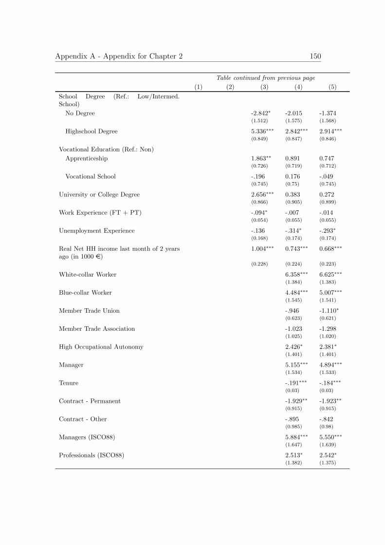
Appendix A - Appendix for Chapter 2 150
Table continued from previous page
(1) (2) (3) (4) (5)
School Degree (Ref.: Low/Intermed.School)
No Degree -2.842∗ -2.015 -1.374(1.512) (1.575) (1.568)
Highschool Degree 5.336∗∗∗ 2.842∗∗∗ 2.914∗∗∗
(0.849) (0.847) (0.846)
Vocational Education (Ref.: Non)
Apprenticeship 1.863∗∗ 0.891 0.747(0.726) (0.719) (0.712)
Vocational School -.196 0.176 -.049(0.745) (0.75) (0.745)
University or College Degree 2.656∗∗∗ 0.383 0.272(0.866) (0.905) (0.899)
Work Experience (FT + PT) -.094∗ -.007 -.014(0.054) (0.055) (0.055)
Unemployment Experience -.136 -.314∗ -.293∗
(0.168) (0.174) (0.174)
Real Net HH income last month of 2 yearsago (in 1000 e)
1.004∗∗∗ 0.743∗∗∗ 0.668∗∗∗
(0.228) (0.224) (0.223)
White-collar Worker 6.358∗∗∗ 6.625∗∗∗
(1.384) (1.383)
Blue-collar Worker 4.484∗∗∗ 5.007∗∗∗
(1.545) (1.541)
Member Trade Union -.946 -1.110∗
(0.623) (0.621)
Member Trade Association -1.023 -1.298(1.025) (1.020)
High Occupational Autonomy 2.426∗ 2.381∗
(1.401) (1.401)
Manager 5.155∗∗∗ 4.894∗∗∗
(1.534) (1.533)
Tenure -.191∗∗∗ -.184∗∗∗
(0.03) (0.03)
Contract - Permanent -1.929∗∗ -1.923∗∗
(0.915) (0.915)
Contract - Other -.895 -.842(0.985) (0.98)
Managers (ISCO88) 5.884∗∗∗ 5.550∗∗∗
(1.647) (1.639)
Professionals (ISCO88) 2.513∗ 2.542∗
(1.382) (1.375)

Appendix A - Appendix for Chapter 2 151
Table continued from previous page
(1) (2) (3) (4) (5)
Technicians and associate professionals(ISCO88)
2.745∗∗ 2.758∗∗∗
(1.072) (1.067)
Clerical support workers (ISCO88) 2.862∗∗ 2.895∗∗
(1.173) (1.165)
Service and sales workers (ISCO88) 0.983 0.936(1.064) (1.059)
Skilled agricultural, forestry and fisheryworkers (ISCO88)
-.288 -.230
(2.575) (2.555)
Craft and related trades workers (ISCO88) -1.010 -1.139(1.013) (1.010)
Plant and machine operators, and assem-blers (ISCO88)
-2.006∗ -2.049∗
(1.079) (1.072)
Firm size small -.925 -.814(0.664) (0.662)
Firm size medium -.790 -.709(0.717) (0.714)
Manufacturing (NACE) 3.092∗∗∗ 3.361∗∗∗
(1.149) (1.144)
Agriculture (NACE) -.680 -.070(2.098) (2.068)
Mining, Quarring, Energy, Water (NACE) 1.168 1.008(1.981) (1.974)
Chemicals/Pulp/Paper (NACE) 3.424∗∗∗ 3.581∗∗∗
(1.326) (1.317)
Construction (NACE) 1.833 1.747(1.322) (1.322)
Iron/Steel (NACE) 0.808 1.060(1.357) (1.350)
Textile/Apparel (NACE) 2.458 2.962(2.191) (2.214)
Wholesale/Retail (NACE) 0.743 0.992(1.126) (1.120)
Transportation/Communication (NACE) -.703 -.620(1.435) (1.435)
Public Service (NACE) -2.811∗∗∗ -2.607∗∗∗
(1.011) (1.003)
Financials/Private Services (NACE) 3.267∗∗∗ 3.387∗∗∗
(1.177) (1.169)
Big Five Factor Openness 0.805∗∗∗

Appendix A - Appendix for Chapter 2 152
Table continued from previous page
(1) (2) (3) (4) (5)(0.257)
Big Five Factor Conscientiousness -.086(0.377)
Big Five Factor Extraversion 0.958∗∗∗
(0.267)
Big Five Factor Agreeableness -1.349∗∗∗
(0.311)
Big Five Factor Neuroticism -.869∗∗∗
(0.251)
Const. 14.653∗∗∗ 17.358∗∗∗ 40.066∗∗∗ 40.382∗∗∗ 41.866∗∗∗
(0.291) (2.204) (2.876) (3.476) (4.425)
Obs. 10972 10972 10972 10972 10972
R2 0.018 0.038 0.128 0.173 0.179
Source: Socio-Economic Panel (SOEP), data for years 1999 - 2008, version 29, SOEP, 2013,
doi: 10.5684/soep.v29, own calculations.
Notes: ∗ p < 0.1, ∗∗ p < 0.05, ∗∗∗ p < 0.01. Standard errors are clustered on person-level.

Appendix A - Appendix for Chapter 2 153
Table A.4: OLS Estimation Results: Gross Log Hourly Wage Income (t+1)
(1) (2) (3) (4) (5)
Locus of Control (std.) 0.057∗∗∗ 0.057∗∗∗ 0.024∗∗∗ 0.015∗∗∗ 0.015∗∗∗
(0.006) (0.006) (0.005) (0.004) (0.004)
General Training 0.195∗∗∗ 0.195∗∗∗ 0.113∗∗∗ 0.044∗∗∗ 0.045∗∗∗
(0.013) (0.013) (0.011) (0.009) (0.009)
Specific Training 0.178∗∗∗ 0.189∗∗∗ 0.094∗∗∗ 0.03∗∗∗ 0.03∗∗∗
(0.014) (0.014) (0.012) (0.01) (0.01)
General Training * Locus of Control (std.) 0.022 0.01 -.006 -.003 -.002(0.014) (0.014) (0.012) (0.01) (0.01)
Specific Training * Locus of Control (std.) -.009 -.018 -.004 -.013 -.014(0.016) (0.015) (0.012) (0.011) (0.011)
East Germany -.176∗∗∗ -.201∗∗∗ -.173∗∗∗ -.173∗∗∗
(0.027) (0.022) (0.019) (0.019)
South Germany -.012 -.014 -.001 -.003(0.016) (0.013) (0.012) (0.012)
North Germany 0.021 0.009 0.007 0.007(0.02) (0.015) (0.013) (0.013)
City States 0.06∗∗ 0.095∗∗∗ 0.072∗∗∗ 0.072∗∗∗
(0.027) (0.022) (0.018) (0.018)
Unemployment Rate -.003 -.005∗∗ -.005∗∗ -.005∗∗
(0.003) (0.002) (0.002) (0.002)
GDP 0.008∗∗∗ 0.005∗∗∗ 0.003∗∗∗ 0.003∗∗∗
(0.001) (0.0009) (0.0008) (0.0008)
Dummy for year 2000 0.045∗∗∗ 0.079∗∗∗ 0.086∗∗∗ 0.085∗∗∗
(0.012) (0.01) (0.018) (0.018)
Dummy for year 2004 0.073∗∗∗ 0.094∗∗∗ 0.102∗∗∗ 0.101∗∗∗
(0.013) (0.01) (0.018) (0.018)
Age -.006∗∗∗ -.004∗∗∗ -.004∗∗∗
(0.001) (0.001) (0.001)
Female -.199∗∗∗ -.154∗∗∗ -.150∗∗∗
(0.009) (0.009) (0.01)
Married -.042∗∗∗ -.012 -.011(0.011) (0.01) (0.01)
Number of Children 0.032∗∗∗ 0.027∗∗∗ 0.028∗∗∗
(0.005) (0.005) (0.005)
Disabled 0.004 -.022 -.021(0.02) (0.018) (0.018)
German Nationality 0.012 -.006 -.007(0.015) (0.013) (0.013)
Owner of House/Dwelling 0.011 0.0004 -.0004(0.009) (0.008) (0.008)

Appendix A - Appendix for Chapter 2 154
Table continued from previous page
(1) (2) (3) (4) (5)
School Degree (Ref.: Low/Intermed.School)
No Degree -.118∗∗ -.077∗ -.076∗
(0.049) (0.043) (0.043)
Highschool Degree 0.179∗∗∗ 0.078∗∗∗ 0.077∗∗∗
(0.014) (0.012) (0.012)
Vocational Education (Ref.: Non)
Apprenticeship 0.03∗∗ 0.029∗∗ 0.029∗∗∗
(0.013) (0.011) (0.011)
Vocational School 0.055∗∗∗ 0.021∗ 0.021∗
(0.014) (0.012) (0.012)
University or College Degree 0.223∗∗∗ 0.088∗∗∗ 0.089∗∗∗
(0.015) (0.014) (0.014)
Work Experience (FT + PT) 0.013∗∗∗ 0.007∗∗∗ 0.007∗∗∗
(0.001) (0.001) (0.001)
Unemployment Experience -.043∗∗∗ -.018∗∗∗ -.018∗∗∗
(0.004) (0.004) (0.004)
White-collar Worker 0.032 0.032(0.022) (0.022)
Blue-collar Worker -.035 -.035(0.023) (0.023)
Member Trade Union 0.038∗∗∗ 0.038∗∗∗
(0.008) (0.008)
Member Trade Association 0.006 0.005(0.015) (0.015)
High Occupational Autonomy 0.078∗∗∗ 0.078∗∗∗
(0.021) (0.021)
Manager 0.103∗∗∗ 0.102∗∗∗
(0.023) (0.023)
Tenure 0.005∗∗∗ 0.005∗∗∗
(0.0005) (0.0005)
Contract - Permanent 0.022 0.021(0.018) (0.018)
Contract - Other -.168∗∗∗ -.168∗∗∗
(0.022) (0.022)
Managers (ISCO88) 0.262∗∗∗ 0.263∗∗∗
(0.024) (0.025)
Professionals (ISCO88) 0.276∗∗∗ 0.276∗∗∗
(0.022) (0.022)
Technicians and associate professionals(ISCO88)
0.235∗∗∗ 0.236∗∗∗
(0.019) (0.019)

Appendix A - Appendix for Chapter 2 155
Table continued from previous page
(1) (2) (3) (4) (5)
Clerical support workers (ISCO88) 0.164∗∗∗ 0.165∗∗∗
(0.02) (0.02)
Service and sales workers (ISCO88) -.001 -.0004(0.02) (0.02)
Skilled agricultural, forestry and fisheryworkers (ISCO88)
0.067 0.071
(0.074) (0.074)
Craft and related trades workers (ISCO88) 0.146∗∗∗ 0.145∗∗∗
(0.018) (0.018)
Plant and machine operators, and assem-blers (ISCO88)
0.099∗∗∗ 0.099∗∗∗
(0.019) (0.019)
Firm size small -.153∗∗∗ -.153∗∗∗
(0.009) (0.009)
Firm size medium -.037∗∗∗ -.037∗∗∗
(0.009) (0.009)
Manufacturing (NACE) 0.075∗∗∗ 0.075∗∗∗
(0.018) (0.018)
Agriculture (NACE) -.139∗∗∗ -.142∗∗∗
(0.051) (0.051)
Mining, Quarring, Energy, Water (NACE) 0.111∗∗∗ 0.111∗∗∗
(0.03) (0.03)
Chemicals/Pulp/Paper (NACE) 0.093∗∗∗ 0.092∗∗∗
(0.021) (0.021)
Construction (NACE) 0.027 0.026(0.02) (0.02)
Iron/Steel (NACE) 0.085∗∗∗ 0.085∗∗∗
(0.021) (0.021)
Textile/Apparel (NACE) -.051 -.048(0.039) (0.04)
Wholesale/Retail (NACE) -.062∗∗∗ -.062∗∗∗
(0.019) (0.019)
Transportation/Communication (NACE) -.015 -.015(0.023) (0.023)
Public Service (NACE) 0.041∗∗ 0.041∗∗
(0.017) (0.017)
Financials/Private Services (NACE) 0.021 0.022(0.019) (0.019)
Big Five Factor Openness 0.0009(0.004)
Big Five Factor Conscientiousness 0.003(0.006)

Appendix A - Appendix for Chapter 2 156
Table continued from previous page
(1) (2) (3) (4) (5)
Big Five Factor Extraversion -.007(0.004)
Big Five Factor Agreeableness -.007(0.005)
Big Five Factor Neuroticism -.004(0.004)
Const. 2.513∗∗∗ 2.324∗∗∗ 2.232∗∗∗ 2.195∗∗∗ 2.262∗∗∗
(0.007) (0.043) (0.051) (0.057) (0.07)
Obs. 10234 10234 10234 10234 10234
R2 0.057 0.135 0.414 0.54 0.54
Source: Socio-Economic Panel (SOEP), data for years 1999 - 2008, version 29, SOEP, 2013, doi: 10.5684/soep.v29,
own calculations.
Notes: ∗ p < 0.1, ∗∗ p < 0.05, ∗∗∗ p < 0.01. Standard Errors are clustered on person-level.

Appendix A - Appendix for Chapter 2 157
Figure A.1: Locus of Control: Factor Analysis and Distribution
item1
item2
item3
item5
item6
item7
item8
item10
-.10
.1.2
.3.4
Fact
or 2
-.4 -.2 0 .2 .4 .6Factor Loading Plot (Locus of Control Items 1999)
Rotation: orthogonal varimaxMethod: principal factors
A
item1
item2
item3
item5
item6
item7
item8
item10
-.10
.1.2
.3.4
Fact
or 2
-.4 -.2 0 .2 .4 .6Factor Loading Plot (Locus of Control Items 2005)
Rotation: orthogonal varimaxMethod: principal factors
B
0.1
.2.3
.4.5
Den
sity
-4 -2 0 2Locus of Control (1999)
C
0.1
.2.3
.4D
ensi
ty
-4 -2 0 2Locus of Control (2005)
D
Source: Socio-Economic Panel (SOEP), data for years 1999 - 2008, version 29, SOEP, 2013, doi:10.5684/soep.v29, own illustration.Notes: Figure 2 A. (B.) shows the loading plot of a factor analysis of the locus of control items of the year 1999(2005). We identify items 1 and 6 as loading on Factor 2 (interpretable as internal factor) and items 2, 3, 5, 7,8, 10 as loading on Factor 1 (interpretable as external factor). Item 4 and 9 are not loading on any of the twofactors and were therefore neglected in the analysis.Figure 2 C. and 2 D. show the distribution of the continuous standardized locus of control index for the years1999 and 2005, which is calculated by firstly reversing all external items and secondly by extracting a singlefactor by running a factor analysis for each year. Hence, higher scores reflect higher internality and lowerscores reflect higher externality. The original item scale of the year 1999 was reversed (in order of higher scoresreflecting higher internality) and was recoded in order to match the locus of control scale of the year 2005. Therecoding is as follows: 2 to 3, 3 to 5 ad 4 to 7.

Appendix A - Appendix for Chapter 2 158

Appendix B - Appendix forChapter 3
Table B.1: List of Countries Used for Cross-Country Analysis
(1) (2) (3) (4)
ISO Code Country % Couples Living % Couples Living
with Wife’s Parents with Husband’s
Parents
mean mean
KHM Cambodia 15.05 5.36
CUB Cuba 8.22 5.02
COL Colombia 7.08 4.87
CHL Chile 4.75 3.29
PER Peru 6.89 4.79
HTI Haiti 5.02 3.63
THA Thailand 9.79 7.31
BRA Brazil 4.60 3.65
IDN Indonesia 10.70 8.55
LAO Lao PDR 16.40 13.30
PHL Philippines 7.49 7.08
UKR Ukraine 5.75 5.53
BOL Bolivia 3.73 3.65
SLV El Salvador 6.14 6.09
PRY Paraguay 4.55 4.65
MWI Malawi 2.44 2.78
ZMB Zambia 2.23 2.69
MEX Mexico 4.53 5.59
HND Honduras 5.17 6.66
GHA Ghana 2.10 3.16
RWA Rwanda 0.39 0.86
COD Congo, Dem. Rep. 3.29 4.84
BDI Burundi 0.23 0.89
AGO Angola 1.82 3.10
159

Appendix B - Appendix for Chapter 3 160
Table continued from previous page
(1) (2) (3) (4)
ISO Code Country % Couples Living % Couples Living
with Wife’s Parents with Husband’s
Parents
mean mean
MDG Madagascar 2.22 3.92
GTM Guatemala 5.62 10.80
SOM Somalia 2.42 5.65
ETH Ethiopia 2.28 5.61
TCD Chad 1.66 4.52
MOZ Mozambique 2.11 6.09
SDN Sudan 3.27 9.84
UGA Uganda 1.09 3.66
TZA Tanzania 2.11 6.89
SLE Sierra Leone 3.78 13.75
CMR Cameroon 1.95 7.14
KAZ Kazakhstan 3.36 13.70
TGO Togo 1.79 6.87
ZWE Zimbabwe 1.92 7.49
BEN Benin 1.47 6.85
VNM Vietnam 3.83 18.95
CIV Cote d’Ivoire 1.76 7.53
TUR Turkey 2.48 13.65
KEN Kenya 0.68 4.09
NGA Nigeria 0.83 5.56
BGD Bangladesh 3.97 26.98
MAR Morocco 2.58 17.80
TUN Tunisia 0.99 6.84
CHN China 1.22 17.60
IRN Iran, Islamic Rep. 0.82 6.48
YEM Yemen, Rep. 2.73 22.20
JOR Jordan 0.91 8.77
KGZ Kyrgyz Republic 2.29 21.65
EGY Egypt, Arab Rep. 1.12 12.11
GIN Guinea 1.29 13.65
MLI Mali 0.41 5.57
AZE Azerbaijan 2.17 25.20
SEN Senegal 2.54 30.16
IND India 2.12 31.45
BFA Burkina Faso 0.61 10.36
NPL Nepal 1.98 30.73
NER Niger 0.53 10.87
DZA Algeria 0.81 16.00

Appendix B - Appendix for Chapter 3 161
Table continued from previous page
(1) (2) (3) (4)
ISO Code Country % Couples Living % Couples Living
with Wife’s Parents with Husband’s
Parents
mean mean
PAK Pakistan 1.84 36.60
UZB Uzbekistan 1.22 30.00
IRQ Iraq 0.88 24.70
TKM Turkmenistan 1.03 30.60
AFG Afghanistan 1.17 34.70
TJK Tajikistan 0.83 37.75
Source: Data from Global Data Lab (https://globaldatalab.org/areadata/patrilocal/).
Notes: This table contains the 68 countries included in Figure 3.1. They have a
population greater than 5 million and at least one data point on co-residence with parents
between 2000 and 2016. We take the mean if there are several data points.

Appendix B - Appendix for Chapter 3 162
Table B.2: Non-Parametric Differences in Pre-Marriage Characteristics
(1) (2) (3) (4) (5)
Treated Controls Difference S.E. T-Stat
A. Wife
Age at marriagec 21.35 20.84 0.51 0.82 0.62
Kyrgyz 0.64 0.69 -0.05 0.11 -0.45
Uzbek 0.15 0.18 -0.03 0.09 -0.33
Dungan 0.10 0.08 0.03 0.06 0.5
Russian 0.05 0.03 0.03 0.04 0.75
Other ethnicity 0.15 0.10 0.05 0.07 0.70
Total number of siblingsc 3.36 3.88 -0.52 0.47 -1.11
Years of educationc 11.00 10.97 0.03 0.49 0.06
More than 11 years of education 0.28 0.36 -0.08 0.11 -0.73
Worked in t-1 if t=year of marriage 0.23 0.26 -0.03 0.11 -0.27
Worked in t-2 if t=year of marriage 0.10 0.23 -0.13 0.10 -1.30
Love marriage 0.70 0.74 -0.04 0.14 -0.29
Arranged marriage 0.26 0.12 0.13 0.11 1.18
Bride capture 0.04 0.13 -0.09 0.09 -1.00
B. Husband
Age at marriagec 25.32 25.49 -0.16 1.10 -0.15
Kyrgyz 0.64 0.69 -0.05 0.11 -0.45
Uzbek 0.15 0.18 -0.03 0.09 -0.33
Dungan 0.10 0.08 0.03 0.06 0.50
Russian 0.03 0.03 0.00 0.04 0.00
Other ethnicity 0.18 0.10 0.08 0.08 1.00
Total number of siblingsc 3.64 3.85 -0.21 0.40 -0.52
Years of educationc 10.92 10.78 0.14 0.45 0.31
More than 11 years of education 0.31 0.28 0.03 0.11 0.27
Worked in t-1 if t=year of marriage 0.82 0.82 0.00 0.1 0.00
Worked in t-2 if t=year of marriage 0.86 0.68 0.18 0.11 1.64
Source: Life in Kyrgyzstan (LIK) Survey, wave 2011, own calculations.Notes: c denotes continuous variable.
Panel A compares pre-marriage characteristics of women married to youngest sons (treated) and not married
to youngest sons (control). Panel B compares pre-marriage characteristics of husbands being youngest sons
(treated) and not being youngest sons (control). Comparisons are based on matching results, whereby the
variable youngest son is used as treatment. The following information are used for balancing: number of
brothers of the husband, age of the husband and age of the oldest living parent of the husband (and
ethnicity, but only if the type of marriage is outcome variable). Column (1) (column (2)) provides the average
treatment effect of the treated (controls), column (3) their difference. Column (4) provides the standard
error and column (5) the t-statistic. Critical values of t-distribution: t∞,0.95 = 1.645, t∞,0.975 = 1.96,
t∞,0.995 = 2.576.

Appendix B - Appendix for Chapter 3 163
Table B.3: Number Of Children Up To Age Five
OLS Estimation Results
Married to youngest son 0.117∗∗
(0.059)
Age husband -.040∗∗∗
(0.004)
No. of brothers (husband) 0.039∗∗
(0.02)
Age oldest living parent (husband) -.0006(0.004)
Const. 2.201∗∗∗
(0.154)
Observations 1,048
Source: Life in Kyrgyzstan (LIK) Survey, wave 2011,own calculations.Notes: Standard errors in parentheses. ∗ p < 0.1, ∗∗
p < 0.05, ∗∗∗ p < 0.01.

Appendix B - Appendix for Chapter 3 164
Table B.4: Estimation Results: Number of Children up to Age 5
(1) (2) (3) (4) (5)
A. OLS Estimation Results
(Co-residence exogenous)
Co-residence 0.334∗∗∗ -.046 -.032 -.013 -.017(0.051) (0.057) (0.056) (0.057) (0.058)
B. Two-stage Least-Squares Estimation Results
(Co-residence endogenous)
Second Stage
Co-residence 0.596∗∗∗ 0.573∗ 0.567∗∗ 0.558∗∗ 0.553∗∗
(0.171) (0.307) (0.281) (0.277) (0.279)
Observations 1,048 1,048 1,048 1,048 1,048
Conditioning Variables X X X X
Wife Characteristics X X X
Residence Characteristics X X
Husband Characteristics X
Source: Life in Kyrgyzstan (LIK) Survey, wave 2011, own calculations.Notes: Standard errors in parentheses. ∗ p < 0.1, ∗∗ p < 0.05, ∗∗∗ p < 0.01.Conditioning variables: age of the husband, number of brothers of the husband, age of the oldest living parent ofthe husband.Wife characteristics: age, educational attainment, ethnicity.Residence characteristics: province, community is urban, availability of kindergarten.Husband characteristics: educational attainment.

Appendix B - Appendix for Chapter 3 165
Table B.5: OLS Estimation Results: Labour Force Participation
(1) (2) (3) (4) (5)Co-residence -.168∗∗∗ -.057 -.023 -.054 -.055
(0.03) (0.036) (0.037) (0.037) (0.037)
Age husband 0.012∗∗∗ -.003 -.005 -.005(0.003) (0.005) (0.005) (0.005)
No. of brothers (husband) 0.003 0.005 0.004 0.004(0.011) (0.011) (0.011) (0.011)
Age oldest living parent (husband) -.0002 -.0007 0.0008 0.0008(0.002) (0.002) (0.002) (0.002)
Age woman 0.047∗∗∗ 0.043∗∗∗ 0.043∗∗∗(0.016) (0.016) (0.016)
Age woman2 -.0004∗∗ -.0004∗ -.0004∗(0.0002) (0.0002) (0.0002)
Medium school education 0.175∗∗∗ 0.157∗∗∗ 0.168∗∗∗(0.054) (0.054) (0.056)
Higher school education 0.273∗∗∗ 0.282∗∗∗ 0.29∗∗∗(0.059) (0.059) (0.062)
Kyrgyz 0.068 -.008 -.008(0.084) (0.087) (0.087)
Uzbek 0.105 0.047 0.045(0.091) (0.097) (0.097)
Dungan -.074 -.086 -.087(0.109) (0.111) (0.111)
Other ethnicity -.049 -.116 -.117(0.1) (0.099) (0.099)
Issyk Kul 0.011 0.014(0.067) (0.067)
Jalalabad 0.003 0.005(0.057) (0.058)
Naryn -.014 -.009(0.081) (0.082)
Batken 0.111 0.112(0.069) (0.069)
Osh 0.177∗∗∗ 0.177∗∗∗(0.054) (0.054)
Talas 0.225∗∗∗ 0.228∗∗∗(0.081) (0.082)
Osh (city) -.068 -.066(0.096) (0.096)
Bishkek (city) 0.101 0.104(0.073) (0.073)
Community in urban area -.113∗∗ -.116∗∗(0.05) (0.05)
Kindergarten in community 0.037 0.038(0.035) (0.036)
Medium school education (husband) -.032(0.048)
Higher school education (husband) -.022(0.055)
Const. 0.558∗∗∗ 0.07 -.638∗∗ -.576∗∗ -.560∗∗(0.021) (0.109) (0.279) (0.278) (0.28)
Observations 1,048 1,048 1,048 1,048 1,048
Source: Life in Kyrgyzstan (LIK) Survey, wave 2011, own calculations.Notes:Standard errors in parentheses. ∗ p < 0.1, ∗∗ p < 0.05, ∗∗∗ p < 0.01.
Russian and Chui are the reference groups for ethnicity and provinces, respectively.

Appendix B - Appendix for Chapter 3 166
Table B.6: Two-stage Least-Squares Estimation Results: Co-Residence (FirstStage)
(1) (2) (3) (4) (5)Married to youngest son 0.316∗∗∗ 0.204∗∗∗ 0.21∗∗∗ 0.213∗∗∗ 0.211∗∗∗
(0.031) (0.032) (0.031) (0.03) (0.03)
Age husband -.033∗∗∗ -.014∗∗∗ -.014∗∗∗ -.014∗∗∗(0.002) (0.004) (0.004) (0.004)
No. of brothers (husband) -.006 -.006 -.007 -.009(0.011) (0.01) (0.01) (0.01)
Age oldest living parent (husband) 0.004∗∗ 0.004∗∗ 0.005∗∗ 0.005∗∗∗(0.002) (0.002) (0.002) (0.002)
Age woman -.104∗∗∗ -.102∗∗∗ -.103∗∗∗(0.013) (0.013) (0.013)
Age woman2 0.001∗∗∗ 0.001∗∗∗ 0.001∗∗∗(0.0002) (0.0002) (0.0002)
Medium school education 0.073 0.059 0.077∗(0.045) (0.044) (0.046)
Higher school education 0.086∗ 0.106∗∗ 0.132∗∗∗(0.049) (0.048) (0.05)
Kyrgyz 0.081 -.050 -.055(0.07) (0.072) (0.072)
Uzbek 0.143∗ -.045 -.057(0.076) (0.08) (0.08)
Dungan 0.141 0.09 0.076(0.091) (0.091) (0.091)
Other ethnicity 0.129 0.035 0.029(0.083) (0.082) (0.082)
Issyk Kul 0.023 0.023(0.055) (0.055)
Jalalabad 0.095∗∗ 0.093∗(0.047) (0.047)
Naryn 0.185∗∗∗ 0.182∗∗∗(0.066) (0.067)
Batken 0.055 0.052(0.057) (0.057)
Osh 0.216∗∗∗ 0.211∗∗∗(0.044) (0.044)
Talas 0.039 0.034(0.067) (0.068)
Osh (city) 0.118 0.117(0.079) (0.079)
Bishkek (city) -.113∗ -.107∗(0.06) (0.06)
Community in urban area -.025 -.025(0.041) (0.041)
Kindergarten in community 0.014 0.018(0.029) (0.029)
Medium school education (husband) -.051(0.04)
Higher school education (husband) -.083∗(0.045)
Const. 0.368∗∗∗ 1.358∗∗∗ 2.474∗∗∗ 2.458∗∗∗ 2.495∗∗∗(0.018) (0.082) (0.22) (0.216) (0.217)
Observations 1,048 1,048 1,048 1,048 1,048
Source: Life in Kyrgyzstan (LIK) Survey, wave 2011, own calculations.Notes: Standard errors in parentheses. ∗ p < 0.1, ∗∗ p < 0.05, ∗∗∗ p < 0.01.
Russian and Chui are the reference groups for ethnicity and provinces, respectively.

Appendix B - Appendix for Chapter 3 167
Table B.7: Two-stage Least-Squares Estimation Results: Labour Force Participa-tion (Second Stage)
(1) (2) (3) (4) (5)Co-residence -.196∗ -.084 -.105 -.045 -.048
(0.101) (0.185) (0.175) (0.17) (0.172)
Age husband 0.011 -.005 -.005 -.005(0.008) (0.006) (0.006) (0.006)
No. of brothers (husband) 0.002 0.002 0.005 0.004(0.013) (0.013) (0.013) (0.013)
Age oldest living parent (husband) 0.00002 0.00007 0.0007 0.0008(0.003) (0.003) (0.003) (0.003)
Age woman 0.039 0.044∗ 0.044∗(0.024) (0.023) (0.023)
Age woman2 -.0003 -.0004 -.0004(0.0003) (0.0003) (0.0003)
Medium school education 0.182∗∗∗ 0.157∗∗∗ 0.167∗∗∗(0.056) (0.055) (0.058)
Higher school education 0.281∗∗∗ 0.281∗∗∗ 0.289∗∗∗(0.061) (0.061) (0.066)
Kyrgyz 0.071 -.007 -.008(0.084) (0.087) (0.087)
Uzbek 0.113 0.047 0.046(0.092) (0.096) (0.097)
Dungan -.065 -.086 -.088(0.11) (0.11) (0.11)
Other ethnicities -.043 -.116 -.117(0.1) (0.098) (0.098)
Issyk Kul 0.011 0.014(0.066) (0.066)
Jalalabad 0.002 0.005(0.058) (0.058)
Naryn -.015 -.011(0.086) (0.086)
Batken 0.11 0.111(0.068) (0.068)
Osh 0.175∗∗∗ 0.176∗∗∗(0.062) (0.062)
Talas 0.225∗∗∗ 0.228∗∗∗(0.08) (0.081)
Osh (city) -.068 -.067(0.096) (0.096)
Bishkek (city) 0.102 0.104(0.076) (0.076)
Community in urban area -.112∗∗ -.115∗∗(0.05) (0.05)
Kindergarten in community 0.037 0.037(0.035) (0.035)
Medium school education (husband) -.032(0.049)
Higher school education (husband) -.022(0.056)
Const. 0.571∗∗∗ 0.106 -.436 -.598 -.577(0.051) (0.267) (0.508) (0.493) (0.503)
Observations 1,048 1,048 1,048 1,048 1,048
Source: Life in Kyrgyzstan (LIK) Survey, wave 2011, own calculations.Notes: Standard errors in parentheses. ∗ p < 0.1, ∗∗ p < 0.05, ∗∗∗ p < 0.01.
Russian and Chui are the reference groups for ethnicity and provinces, respectively.

Appendix B - Appendix for Chapter 3 168
Table B.8: Tobit Estimation Results: Working Hours
(1) (2) (3) (4) (5)Co-residence -14.241∗∗∗ -4.388 -1.241 -3.220 -3.319
(2.672) (3.131) (3.180) (3.218) (3.228)
Age husband 1.118∗∗∗ -.004 -.138 -.136(0.258) (0.467) (0.462) (0.463)
No. of brothers (husband) 0.29 0.505 0.68 0.672(0.964) (0.974) (0.96) (0.963)
Age oldest living parent (husband) -.082 -.125 0.021 0.023(0.195) (0.194) (0.193) (0.194)
Age woman 5.087∗∗∗ 4.721∗∗∗ 4.722∗∗∗(1.439) (1.414) (1.418)
Age woman2 -.056∗∗∗ -.051∗∗∗ -.051∗∗∗(0.019) (0.019) (0.019)
Medium school education 14.336∗∗∗ 13.817∗∗∗ 14.767∗∗∗(5.214) (5.186) (5.429)
Higher school education 22.496∗∗∗ 22.935∗∗∗ 23.522∗∗∗(5.530) (5.542) (5.806)
Kyrgyz 1.777 -.997 -.997(7.317) (7.466) (7.472)
Uzbek 7.275 4.384 4.293(7.894) (8.315) (8.350)
Dungan -14.548 -12.761 -12.704(10.350) (10.358) (10.389)
Other ethnicity -7.550 -11.423 -11.372(8.833) (8.740) (8.752)
Issyk Kul -6.762 -6.400(5.924) (5.944)
Jalalabad -3.693 -3.414(5.105) (5.123)
Naryn -3.674 -3.093(7.341) (7.385)
Batken 2.432 2.524(6.058) (6.064)
Osh 13.799∗∗∗ 13.898∗∗∗(4.762) (4.769)
Talas 14.800∗∗ 15.205∗∗(6.801) (6.836)
Osh (city) -10.166 -9.901(8.848) (8.851)
Bishkek (city) 9.390 9.580(6.315) (6.324)
Community in urban area -2.901 -3.207(4.357) (4.380)
Kindergarten in community 0.952 0.912(3.076) (3.083)
Medium school education (husband) -2.796(4.306)
Higher school education (husband) -1.361(4.774)
Const. 6.661∗∗∗ -34.123∗∗∗ -112.226∗∗∗ -110.210∗∗∗ -109.034∗∗∗(1.871) (9.708) (25.336) (25.119) (25.279)
Observations 1,048 1,048 1,048 1,048 1,048
Source: Life in Kyrgyzstan (LIK) Survey, wave 2011, own calculations.Notes: Standard errors in parentheses. ∗ p < 0.1, ∗∗ p < 0.05, ∗∗∗ p < 0.01.
Russian and Chui are the reference groups for ethnicity and provinces, respectively.

Appendix B - Appendix for Chapter 3 169
Table B.9: IV Tobit Estimation Results: Working Hours (Second Stage)
(1) (2) (3) (4) (5)Co-residence -19.731∗∗ -12.161 -15.009 -9.023 -9.193
(8.874) (16.120) (15.528) (14.982) (15.136)
Age husband 0.816 -.265 -.248 -.245(0.666) (0.552) (0.54) (0.538)
No. of brothers (husband) 0.003 0.0007 0.459 0.44(1.130) (1.130) (1.112) (1.128)
Age oldest living parent (husband) -.009 0.01 0.08 0.084(0.245) (0.246) (0.244) (0.248)
Age woman 3.673∗ 4.136∗∗ 4.120∗∗(2.127) (2.044) (2.074)
Age woman2 -.040 -.045∗ -.045∗(0.027) (0.026) (0.026)
Medium school education 15.530∗∗∗ 14.246∗∗∗ 15.322∗∗∗(5.420) (5.306) (5.615)
Higher school education 23.906∗∗∗ 23.648∗∗∗ 24.420∗∗∗(5.793) (5.837) (6.242)
Kyrgyz 2.245 -1.513 -1.546(7.399) (7.589) (7.610)
Uzbek 8.574 3.921 3.745(8.093) (8.409) (8.475)
Dungan -13.057 -12.449 -12.478(10.552) (10.399) (10.416)
Other ethnicity -6.443 -11.485 -11.474(8.990) (8.754) (8.769)
Issyk Kul -6.637 -6.277(5.941) (5.960)
Jalalabad -3.235 -2.965(5.242) (5.254)
Naryn -2.555 -1.977(7.874) (7.910)
Batken 2.682 2.756(6.100) (6.101)
Osh 14.954∗∗∗ 15.039∗∗∗(5.592) (5.576)
Talas 14.767∗∗ 15.141∗∗(6.813) (6.850)
Osh (city) -9.678 -9.415(8.946) (8.947)
Bishkek (city) 8.643 8.862(6.598) (6.585)
Community in urban area -3.024 -3.329(4.375) (4.397)
Kindergarten in community 1.050 1.034(3.091) (3.103)
Medium school education (husband) -3.128(4.393)
Higher school education (husband) -1.905(4.975)
Const. 9.289∗∗ -23.599 -78.151∗ -95.943∗∗ -94.348∗∗(4.442) (23.480) (45.329) (43.840) (44.745)
Observations 1,048 1,048 1,048 1,048 1,048
Source: Life in Kyrgyzstan (LIK) Survey, wave 2011, own calculations.Notes: Standard errors in parentheses. ∗ p < 0.1, ∗∗ p < 0.05, ∗∗∗ p < 0.01.
Russian and Chui are the reference groups for ethnicity and provinces, respectively.

Appendix B - Appendix for Chapter 3 170
Table B.10: Heterogeneity Analysis: Labour Force Participation
(1) (2) (3) (4) (5) (6) (7)A. OLS Estimation Results
(Co-residence exogenous)
Co-residence -.029 0.069 -.224∗∗∗ 0.093 -.077 -.141∗∗∗ -.080(0.041) (0.096) (0.082) (0.212) (0.061) (0.05) (0.075)
Co-residence * Community in urban area -.111(0.071)
Co-residence * Medium school education -.131(0.1)
Co-residence * Higher school education -.147(0.107)
Co-residence * Age woman 20-29 0.205∗∗(0.099)
Co-residence * Age woman 30-39 0.204∗∗(0.096)
Co-residence * Age oldest living parent (husband) -.002(0.003)
Co-residence * Oldest living parent (husband) retired 0.032(0.07)
Co-residence * Number of children up to age 5 0.09∗∗(0.036)
Co-residence * Substitute women 0.062(0.145)
B. Two-Stage Least-Squares Estimation Results(Co-residence endogenous)Second Stage
Co-residence - - -.303 1.181 -.153 -.009 -(0.228) (1.618) (0.498) (0.192)
Co-residence * Community in urban area -
Co-residence * Medium school education -
Co-residence * Higher school education -
Co-residence * Age woman 20-29 0.344(0.366)
Co-residence * Age woman 30-39 0.411(0.264)
Co-residence * Age oldest living parent (husband) -.017(0.021)
Co-residence * Oldest living parent (husband) retired 0.12(0.45)
Co-residence * Number of children up to age 5 0.013(0.134)
Co-residence * Substitute women -
Observations 1,048 1,048 1,048 1,048 1,048 1,048 1,048Conditioning Variables X X X X X X XWife Characteristics X X X X X X XResidence Characteristics X X X X X X XHusband Characteristics X X X X X X X
Source: Life in Kyrgyzstan (LIK) Survey, wave 2011, own calculations.Notes: Standard errors in parentheses. ∗ p < 0.1, ∗∗ p < 0.05, ∗∗∗ p < 0.01.Heterogeneity tests are presented in the different columns. IV estimates are only shown if our instrument issufficiently strong in eachrespective sub-sample. We control for the same set of variables as in our main specifications. We test forheterogeneous resultswith respect to the following variables:(1) Community in urban area (reference category are communities in rural areas).(2) Education of the women (reference category are women with low school education).(3) Age of the women (reference category are women between age 40 and 50).(4) Age of the oldest living parent of the husband.(5) Oldest living parent of the husband is retired (reference category are husbands with the oldest livingparent not being retired).(6) Number of children up to age 5.(7) Substitute women (reference category are households without substitute women).

Appendix B - Appendix for Chapter 3 171
Table B.11: Heterogeneity Analysis: Working Hours
(1) (2) (3) (4) (5) (6) (7)A. Tobit Estimation Results
(Co-residence exogenous)
Co-eesidence -.243 5.823 -17.384∗∗ 14.940 -5.194 -8.834∗∗ -7.758(3.493) (9.426) (6.974) (18.764) (5.460) (4.185) (6.661)
Co-residence * Community in urban area -14.282∗∗(6.355)
Co-residence * Medium school education -7.787(9.716)
Co-residence * Higher school education -12.948(10.159)
Co-residence * Age woman 20-29 18.350∗∗(8.777)
Co-residence * Age woman 30-39 15.999∗∗(8.107)
Co-residence * Age oldest living parent (husband) -.274(0.278)
Co-residence * Oldest living parent (husband) retired 2.587(6.182)
Co-residence * Number of children up to age 5 6.618∗∗(3.254)
Co-residence * Substitute women 7.754(12.833)
B. IV Tobit Estimation Results(Co-residence endogenous)Second Stage
Co-residence - - -29.124 58.064 -34.515 -4.760 -(19.298) (147.069) (47.582) (16.389)
Co-residence * Community in urban area -
Co-residence * Medium school education -
Co-residence * Higher school education -
Co-residence * Age woman 20-29 22.097(33.650)
Co-residence * Age woman 30-39 35.212(22.193)
Co-residence * Age oldest living parent (husband) -.911(1.902)
Co-residence * Oldest living parent (husband) retired 28.193(43.178)
Co-residence * Number of children up to age 5 2.340(12.504)
Co-residence * Substitute women -
Observations 1,048 1,048 1,048 1,048 1,048 1,048 1,048Conditioning Variables X X X X X X XWife Characteristics X X X X X X XResidence Characteristics X X X X X X XHusband Characteristics X X X X X X X
Source: Life in Kyrgyzstan (LIK) Survey, wave 2011, own calculations.Notes: Standard errors in parentheses. ∗ p < 0.1, ∗∗ p < 0.05, ∗∗∗ p < 0.01.Heterogeneity tests are presented in the different columns. IV estimates are only shown if our instrument is sufficientlystrong in each respectivesub-sample. We control for the same set of variables as in our main specifications. We test for heterogeneous results withrespect to the followingvariables:(1) Community in urban area (reference category are communities in rural areas).(2) Education of the women (reference category are women with low school education).(3) Age of the women (reference category are women between age 40 and 50).(4) Age of the oldest living parent of the husband.(5) Oldest living parent of the husband is retired (reference category are husbands with the oldest living parent not beingretired).(6) Number of children up to age 5.(7) Substitute women (reference category are households without substitute women).

Appendix B - Appendix for Chapter 3 172
Table B.12: Summary Statistics of Variables used in Channel Analysis
(1) (2) (3) (4) (5)Observations Mean SD Min Max
A. WomanElder care time (in hours) 1,048 0.13 (0.47) 0.00 6.50Child care time (in hours) 1,048 1.76 (1.97) 0.00 12.00Housekeeping time (in hours) 1,048 5.38 (2.69) 0.00 14.00Leisure time (in hours) 1,048 2.44 (1.77) 0.00 11.00B. Parents or in-lawsIncome parents (in 1000 Som) 501 4.18 (4.84) 0.00 60.00Gender attitudes 490 -0.05 (0.98) -2.86 1.52
Source: Life in Kyrgyzstan (LIK) Survey, wave 2011, own calculations.
Notes: Summary statistics of parents or in-laws are restricted to only co-residing women.
Table B.13: Gender Attitude Items
Gender Attitude Items Liberal/(Scale 1-4) Traditional
I1: Important decisions should be made by the husband rather than the wife TI2: A man’s job is to earn money; a woman’s job is to look after the home and family TI3: A women is really fulfilled only when she becomes a mother TI4: A working women can establish just as warm and secure of relationship with her
children as a mother who does not work LI5: A husband’s career should be more important to the wife than her own TI6: A university education is more important for a boy than for a girl TI7: Both the husband and the wife should contribute to the household income L
Source: Life in Kyrgyzstan (LIK) Individual Questionnaire 2011.
Notes: Items marked with T/L refer to items which are categorized as traditional (T) or liberal (L), meaning the
respondent has a rather traditional/liberal attitude towards the role of females in the society.

Appendix C - Appendix forChapter 4
Table C.1: Panel Attrition 2013-2017
(1) (2) (3) (4) (5) (6)2013 2014 2015 2016 2017 #firms
22038425347
# firms 383 347 292 257 219attrition rate 0.09 0.24 0.33 0.43
Source: Survey on micro and small enterprises in Uganda, waves 2013-2017, own calculations. Numbers refer to the estimation sample.
Notes: The table provides an overview on how long firms stay in the
sample, the number of firms in each year and on panel attrition The
shaded areas refer to the waves in which a firm is observed in the
sample. Based on all firms in the estimation sample in 2013, 220 firms
stay 5 consecutive waves in the panel (row 1), 38 for 4 waves (row
2), 42 for 3 waves (row 3), 53 for 2 waves (row 4) and 46 for 1 wave
only (row 5). The row labelled with ’#firms’ gives the number of firms
which are observed in the respective waves e.g. in 2013 there are 383
firms in the estimation sample. The last row gives the attrition rate.
For example in 2014, 9 percent of firms observed in 2013 are not in
the survey any more.
173

Appendix C - Appendix for Chapter 4 174
Table C.2: Number of Observations on Subitems: Credit Constraints
(1) (2)Formal Informalshare share
A. Credit Constraineda
Expected rejection 20.93 8.96Unfamiliar with process 9.77 2.05Does not know source 0.93 7.84Uncomfortable 54.19 68.66Not registered 2.09 0.56Unable to pay back 2.79 2.80Rejected 0.93 1.49Not full amount 4.42 4.48Religious reasons 3.95 3.17Sum 100 100
B. Credit Unconstrainedb
Interest rates too high 31.19 15.33Received full amount 33.17 27.20No need 35.64 57.47Sum 100 100
Source: Survey on micro and small enterprises in Uganda,waves 2013-2017, own calculations. Summary statistics re-fer to the estimation sample.Notes:a Shares refer to the total number of credit constrained.b Shares refer to the total number of credit unconstrained.

Appendix C - Appendix for Chapter 4 175
Table C.3: Managerial Constraint Items
(1) (2) (3)Item Abbreviation Item Survey Question
Gift sharing s2 Imagine that five brothers are given a gift of 10,000,000 UGX.If the brothers have to share the money equally how muchdoes each one get?
Inflation s3 Imagine that you get a gift of 300,000 UGX, and you put itat home for 12 months. Inflation stays at 10%. After oneyear, how much could you buy for this money?
Zero interest s4 You lend 100,000 UGX to a friend one evening and he givesyou 100,000 UGX back the next month. How much interesthas he paid on this loan?
Interest s5a Suppose you put 100,000 UGX into a savings account witha guaranteed interest rate of 2% per year. You do not haveto pay fees, you don’t make any further payments into thisaccount and you don’t withdraw any money. How muchwould be in the account at the end of the first year, oncethe interest payment is made?
Compound interest s5b How much would be in the account at the end of five years?
s6 I would like to ask you whether you think the followingstatements are true or false
Statement: high return a An investment with high return is likely to be of high risk
Statement: inflation b High inflation means that the cost of living is increasing sharply
Statement: risk diversification c It is less likely that you will lose all of your money if yousave it in more than one place
Statement: agreement d A financial institution needs to get your agreement firstbefore sharing your information with someone else
Discount s7 Imagine the same cell-phone is on sale in two different shopsat 200,000 UGX and one shop offered a discount of30,000 UGX and the other shop offered a 10% discount: whichone is the better bargain?
Source: Survey on micro and small enterprises in Uganda.
Notes: Column (1) shows the item label, Column (2) the item number as used in the survey, Column (3) gives the
exact survey question.

Appendix C - Appendix for Chapter 4 176
Table C.4: Random Effects Estimation Results: Log Investments
(1) (2) (3) (4)Saving Constraint Index -.273∗∗∗ -.160∗∗ -.128 -.153∗
(0.078) (0.079) (0.081) (0.081)
Managerial Constraint Index -.260∗∗∗ -.235∗∗∗ -.202∗∗∗ -.142∗(0.073) (0.074) (0.073) (0.075)
Female -.577∗∗∗ -.238 -.263(0.175) (0.186) (0.187)
Married 0.11 0.018 0.045(0.164) (0.162) (0.16)
Age -.002 -.042 -.056(0.055) (0.066) (0.065)
Age squared -.0004 0.0002 0.0003(0.0006) (0.0008) (0.0008)
No education -1.107∗∗∗ -.721∗∗ -.583(0.35) (0.367) (0.369)
Primary school -.413 -.223 -.123(0.288) (0.31) (0.313)
Completed O-level -.421 -.372 -.284(0.292) (0.296) (0.302)
Completed A-level -.498 -.417 -.372(0.311) (0.31) (0.31)
Cognitive ability (raven score) 0.029 0.015 0.022(0.036) (0.034) (0.034)
Business experience 0.022 0.027 0.013(0.016) (0.052) (0.051)
Planned investment 0.563∗∗∗ 0.519∗∗∗ 0.522∗∗(0.201) (0.199) (0.204)
Age of firm 0.009 -.015(0.063) (0.063)
Age of firm squared -.0008 0.00004(0.001) (0.001)
Initial capital stock (USD) 1.23e-06∗∗∗ 1.59e-06∗∗∗(4.62e-07) (4.90e-07)
Own-account worker -.413∗∗∗ -.444∗∗∗(0.157) (0.158)
Registered with revenue authority 0.535∗∗ 0.433∗(0.221) (0.223)
Services 0.256 0.201(0.367) (0.369)
Manufacturing (textile) -.580 -.573(0.356) (0.357)
Manufacturing (remaining) -.110 -.115(0.385) (0.387)
Retail and Wholesale (remaining) -1.161∗∗∗ -1.142∗∗∗(0.368) (0.368)
Retail and Wholesale (retail, clothing) -.856∗∗ -.797∗∗(0.384) (0.386)
Retail and Wholesale (electric, phones) -.410 -.393(0.438) (0.432)
Remaining sectors -1.058∗ -.991∗(0.559) (0.551)
Year 2014 0.706∗∗∗(0.186)
Year 2015 0.392∗(0.203)
Year 2016 0.378∗(0.225)
Year 2017 1.315∗∗∗(0.234)
Const. 2.890∗∗∗ 3.272∗∗∗ 4.380∗∗∗ 4.352∗∗∗(0.091) (1.189) (1.318) (1.300)
Obs. 1498 1498 1498 1498
Source: Survey on micro and small enterprises in Uganda, waves 2013-2017, own calculations.Notes: Standard errors in parentheses. Standard errors clustered at firm level.∗ p < 0.1, ∗∗ p < 0.05, ∗∗∗ p < 0.01. University and Manufacturing (printing, paper) are thereference groups for education and industry sector, respectively.

Appendix D - Appendix forChapter 5
Table D.1: Overview Training Program
Topic 1 Financial managementSavingsBorrowingConsumption
Topic 2 Business investment and growth strategiesProfitsInvestmentsRisk Diversification
Topic 2 Separating business and household financesImportance of separating moneySetting yourself a salaryRepaying for money or goodsHousehold budget
Table D.2: Statements on Separating Finances
Question Indicator=1(1) “How often do you keep the accounts or books for your business and ” 1= sometimes/almost always
home separate?(2) “How often do you keep cash for your business and home physically separated?” 1= sometimes/almost always(3) “How often do you set money aside for your business but is gets used for
household/private expenses?” 1= never/rarely(4) “If you take money out of your business (apart from the salary you take out)
to pay household/private expenses, how often do you put it back?” 1= sometimes/almost always(5) “If you take goods out of your business for your household/relatives/friends,
does someone (you/relatives/friends) pay for it?” 1= sometimes/almost always(6) “Writing down what you plan to do with your money for your family and
household means you make a household budget. How often do you do that?” 1= sometimes/almost always
Note: This table provides all statements which are used as outcome variables in the “separating finances index”.
177

Appendix D - Appendix for Chapter 5 178
Table D.3: Effect on Aggregates
Average Average Principal Principalover all Indices over all Variables component component
continuous ordinal(1) (2) (3) (4)
Personalized Training 0.26∗∗ 0.255∗∗ 0.217∗ 0.156∗∗(0.117) (0.108) (0.116) (0.079)
Rule-of-Thumb Training 0.181∗ 0.152 0.092 0.06(0.106) (0.094) (0.106) (0.071)
Source: Survey on micro and small enterprises in Uganda, waves 2017-2018, own calculations.
Notes: Standard errors in parentheses. ∗ p < 0.1, ∗∗ p < 0.05, ∗∗∗ p < 0.01.
Table D.4: Separating Finances
Separating QuestionFinances Separating of Business Money Put money back Paying for goods Budget
Index Accounts Cash used for hh if from business taken from business Making(1) (2) (3) (4) (5) (6) (7)
Personalized Training (PT) -.028 0.002 -.046 -.087 0.005 -.003 0.02(0.113) (0.058) (0.056) (0.054) (0.052) (0.055) (0.058)
Rule-of-Thumb Training (RoT) 0.127 0.031 -.005 -.023 0.082∗ 0.041 0.05(0.103) (0.057) (0.056) (0.055) (0.049) (0.054) (0.057)
Const. 0.049 0.493∗∗∗ 0.599∗∗∗ 0.299∗∗∗ 0.628∗∗∗ 0.662∗∗∗ 0.545∗∗∗(0.143) (0.086) (0.078) (0.075) (0.078) (0.078) (0.082)
PT-RoT=0 (p-value) 0.13 0.61 0.47 0.23 0.12 0.42 0.60R2 0.06 0.03 0.01 0.02 0.02 0.01 0.03Mean (SD) of 0.00 0.60 0.00 0.35 0.71 0.63 0.50control group (1.00) (0.49) (1.00) (0.48) (0.45) (0.48) (0.50)Observations 446 446 446 446 446 446 446Control for yt−1 yes yes yes yes yes yes yesControl for industry strata yes yes yes yes yes yes yes
Source: Survey on micro and small enterprises in Uganda, waves 2017-2018, own calculations.Notes: Standard errors in parentheses. ∗ p < 0.1, ∗∗ p < 0.05, ∗∗∗ p < 0.01. An overview of all exact statements used asoutcome variables in Columns (1)-(7) can be found in Table D.2.

Publications 179
Publications
Kapitel 2: Locus of Control and Investment in Training (with Marco Caliendo,
Deboarah Cobb-Clark, Arne Uhlendorff)
• SOEPpapers (2016), No. 890
• IZA Discussion Paper Series (2016), No. 10406
Kapitel 3: Patrilocal Residence and Female Labour Supply: Evidence from Kyr-
gyzstan (with Andreas Landmann und Susan Steiner)
• Landmann, A., Seitz, H. & Steiner, S. Demography (2018) 55: 2181. https:
//doi.org/10.1007/s13524-018-0724-1
• SOEPpapers (2017), No. 1705
• IZA Discussion Paper Series (2017), No. 10890