Essays in Applied Economics - University of Ottawa

Essays in Applied Economics

Kunyu Wang

Thesis submitted to the Faculty of Graduate and Postdoctoral Studies

in partial fulfilment of the requirements for the degree:

Doctorate in Philosophy Economics

Department of Economics

University of Ottawa

Ottawa, Ontario, Canada

c© Kunyu Wang, Ottawa, Canada, 2018

Abstract

Chapter 1 Does the party of government influence the amount and type of in-

ward foreign investment? The results of a number of correlational studies provide

inconsistent evidence. However none of these studies - for any level of government

or any jurisdiction - have used methods that allow them to speak to causal effects.

Regression discontinuity (RD) method is applied to a set of narrow-margin US guber-

natorial elections. Over the course of a four-year term the election of a Republican

governor causes a 21% boost in the growth of manufacturing-oriented FDI stock,

compared to a Democrat. This effect is robust to a series of challenges. However, the

same approach provides no evidence that partisanship matters for the overall level

of FDI.

Chapter 2 Does an economic shock open a window of opportunity for reform, and

if it does, how does the institution of a state play a role? The paper investigates

how economic shocks affect the structural reforms in various institutions. This paper

addresses this issue by using the exogenous variation in the international price of

large commodity goods to generate the exogenous change in national income. The

analysis relies on a unique mapping between new annual data from 1962 to 2005

ii

on economic shocks from commodity prices and structural reforms in 111 countries.

I find significant heterogeneous effects across sectors in autocratic countries. In

autocracies, positive economic shocks promote reforms in real sectors, but deter

reforms in financial sectors. However the impact of economic shocks on structural

reform in democratic countries is nil.

Chapter 3 The deregulation of branch banking across the United States substan-

tially increased the availability of credit to existing borrowers and others who has

previously been excluded. Exploiting the staggered timing of changes across states

for identification it is estimated that deregulation caused a 3.3% increase in rates of

suicide and a 4.7% increase in rates of divorce. This is consistent with a large body

of evidence linking excess debt to various measures of individual and relationship

distress. Results are in most cases statistically significant at levels much higher than

1%, and prove resilient in a battery of robustness checks and falsification exercises.

iii

Acknowledgements

I am grateful to my thesis supervisor, Anthony Heyes for his guidance, encouragement

and advice. I would like to thank my committee members, Zhihao Yu, Roland Pongou

Jason Garred and Anindya Sen, for their reviews and suggestions. I acknowledge

valuable comments by Abel Brodeur, Paul Makdissi, Aggey Semenov, Louis-Philippe

Morin and Pierre Brochu. I would also like to thank Christopher Ksoll, Zhiqi Chen,

Rose Anne Devlin and Victoria Barham for supporting me during my study. The

research reported in chapters 1 and 3 form the basis for coauthored papers with

Anthony Heyes.

iv

Table of Contents

Abstract ii

Acknowledgements iv

General Introduction 1

1 Subnational Politics and Foreign Direct Investment (FDI): First

Causal Evidence 5

1.1 Introduction . . . . . . . . . . . . . . . . . . . . . . . . . . . . . . . . 5

1.2 Research Design . . . . . . . . . . . . . . . . . . . . . . . . . . . . . . 10

1.2.1 Methods . . . . . . . . . . . . . . . . . . . . . . . . . . . . . . 10

1.2.2 Study Setting . . . . . . . . . . . . . . . . . . . . . . . . . . . 15

1.2.3 Data . . . . . . . . . . . . . . . . . . . . . . . . . . . . . . . . 16

1.3 Results . . . . . . . . . . . . . . . . . . . . . . . . . . . . . . . . . . . 19

1.3.1 Main results . . . . . . . . . . . . . . . . . . . . . . . . . . . . 19

1.3.2 Validity . . . . . . . . . . . . . . . . . . . . . . . . . . . . . . 21

1.3.3 Methodological robustness . . . . . . . . . . . . . . . . . . . . 23

1.4 Possible Channels . . . . . . . . . . . . . . . . . . . . . . . . . . . . . 26

1.5 Conclusion . . . . . . . . . . . . . . . . . . . . . . . . . . . . . . . . . 27

2 Commodity Price Shocks, Institutions and Windows of Opportunity

for Structural Reform 44

2.1 Introduction . . . . . . . . . . . . . . . . . . . . . . . . . . . . . . . . 44

2.2 Literature Review . . . . . . . . . . . . . . . . . . . . . . . . . . . . . 47

v

2.3 Data . . . . . . . . . . . . . . . . . . . . . . . . . . . . . . . . . . . . 50

2.3.1 Data on reforms . . . . . . . . . . . . . . . . . . . . . . . . . . 50

2.3.2 Data on commodity prices . . . . . . . . . . . . . . . . . . . . 52

2.3.3 Data on institutions . . . . . . . . . . . . . . . . . . . . . . . 53

2.4 Research Design . . . . . . . . . . . . . . . . . . . . . . . . . . . . . . 54

2.4.1 Empirical Strategy . . . . . . . . . . . . . . . . . . . . . . . . 54

2.4.2 Model . . . . . . . . . . . . . . . . . . . . . . . . . . . . . . . 55

2.5 Results . . . . . . . . . . . . . . . . . . . . . . . . . . . . . . . . . . . 57

2.5.1 Main Results . . . . . . . . . . . . . . . . . . . . . . . . . . . 57

2.5.2 Robustness Checks . . . . . . . . . . . . . . . . . . . . . . . . 60

2.6 Conclusion . . . . . . . . . . . . . . . . . . . . . . . . . . . . . . . . . 62

3 The Social Footprint of Bank Regulation: Natural Experimental

Evidence from the US 72

3.1 Introduction . . . . . . . . . . . . . . . . . . . . . . . . . . . . . . . . 72

3.2 Literature Review . . . . . . . . . . . . . . . . . . . . . . . . . . . . . 76

3.3 Setting . . . . . . . . . . . . . . . . . . . . . . . . . . . . . . . . . . . 79

3.4 Data . . . . . . . . . . . . . . . . . . . . . . . . . . . . . . . . . . . . 80

3.5 Empirical Strategy . . . . . . . . . . . . . . . . . . . . . . . . . . . . 81

3.6 Results . . . . . . . . . . . . . . . . . . . . . . . . . . . . . . . . . . . 83

3.6.1 Main Results: Suicide . . . . . . . . . . . . . . . . . . . . . . 83

3.6.2 Main Results: Divorce . . . . . . . . . . . . . . . . . . . . . . 84

3.6.3 Robustness . . . . . . . . . . . . . . . . . . . . . . . . . . . . 84

3.6.4 Falsification: Evidence from 6000 Placebos . . . . . . . . . . . 88

3.7 Conclusion . . . . . . . . . . . . . . . . . . . . . . . . . . . . . . . . . 91

3.8 Appendix . . . . . . . . . . . . . . . . . . . . . . . . . . . . . . . . . 104

Bibliography 109

vi

List of Tables

1.1 Summary Statistics . . . . . . . . . . . . . . . . . . . . . . . . . . . 29

1.2 Statistics on Gubernatorial Elections . . . . . . . . . . . . . . . . . . 30

1.3 RD Estimates for FDI Per Capita . . . . . . . . . . . . . . . . . . . 31

1.4 RD Estimates for FDI Manufacturing Per Capita . . . . . . . . . . . 32

1.5 Covariate Balance Tests for Gubernatorial RD Design . . . . . . . . 33

1.6 RD Estimates for FDI Manufacturing Per Capita: Senate/House/President

. . . . . . . . . . . . . . . . . . . . . . . . . . . . . . . . . . . . . . . 34

1.7 RD Estimates for FDI Manufacturing Per Capita: 5% & 10% Bandwidth 35

1.8 RD Estimates for FDI Manufacturing Per Capita: Second Order Poly-

nomial . . . . . . . . . . . . . . . . . . . . . . . . . . . . . . . . . . . 36

1.9 RD Estimates for FDI Manufacturing Per Capita: 99% & 95% Win-

sorizing . . . . . . . . . . . . . . . . . . . . . . . . . . . . . . . . . . 37

1.10 RD Estimates for FDI Manufacturing as Percent of GSP . . . . . . . 38

2.1 Summary Statistic . . . . . . . . . . . . . . . . . . . . . . . . . . . . 65

2.2 Estimation for Financial Market Reform . . . . . . . . . . . . . . . . 66

2.3 Estimation for Product Market Reform . . . . . . . . . . . . . . . . 67

2.4 Robustness Check for Financial Market Reform: Exclude Big Pro-

ducer & Big Regulation Indices & Control for Shares . . . . . . . . . 68

2.5 Robustness Check for Product Market Reform: Exclude Big Producer

& Big Regulation Indices & Control for Shares . . . . . . . . . . . . 69

2.6 Robustness Check for Financial Market Reform: Export Share . . . 70

2.7 Robustness Check for Product Market Reform: Export Share . . . . 71

vii

3.1 Year Intrastate Bank Branching First Allowed . . . . . . . . . . . . . 93

3.2 Summary Statistics . . . . . . . . . . . . . . . . . . . . . . . . . . . 94

3.3 Main Result: Suicide . . . . . . . . . . . . . . . . . . . . . . . . . . . 95

3.4 Main Result: Divorce . . . . . . . . . . . . . . . . . . . . . . . . . . . 96

3.5 Robustness Check: Suicide . . . . . . . . . . . . . . . . . . . . . . . 97

3.6 Robustness Check: Divorce . . . . . . . . . . . . . . . . . . . . . . . 98

3.7 Exclude Large States - Suicide . . . . . . . . . . . . . . . . . . . . . . 104

3.8 Exclude Large States - Divorce . . . . . . . . . . . . . . . . . . . . . 105

3.9 Inclusion of Lagged Unemployment Rate - Suicide . . . . . . . . . . . 106

3.10 Inclusion of Lagged Unemployment Rate - Divorce . . . . . . . . . . . 107

viii

List of Figures

1.1 Histogram of victory margin . . . . . . . . . . . . . . . . . . . . . . . 39

1.2 RD estimates on FDI, 1 to 4 years after election . . . . . . . . . . . . 40

1.3 RD estimates on FDI Manufacturing, 1 to 4 years after election . . . 41

1.4 The effect of electing a Republican governor on change in FDI in

Manufacturing . . . . . . . . . . . . . . . . . . . . . . . . . . . . . . . 42

1.5 McCrary density of victory margin . . . . . . . . . . . . . . . . . . . 43

3.1 Timing of intrastate branching deregulation . . . . . . . . . . . . . . 99

3.2 Timing of bank deregulation and pre-existing suicide rate . . . . . . . 100

3.3 Timing of bank deregulation and pre-existing divorce rate . . . . . . . 101

3.4 Suicide placebo tests . . . . . . . . . . . . . . . . . . . . . . . . . . . 102

3.5 Divorce placebo tests . . . . . . . . . . . . . . . . . . . . . . . . . . . 103

3.6 Timing of bank deregulation and unilateral divorce law . . . . . . . . 108

ix

General Introduction

My thesis lies in applied economic analysis on the partisanship effects on foreign

direct investment, commodity price shocks and window of opportunity for structural

reforms, and social costs of bank de-regulation laws. Given the varied nature of these

topics, I apply a diverse set of tools drawn from applied econometrics by exploiting

natural experiments. Establishing causal inference is one of the most pressing chal-

lenges in modern applied economics as oftentimes, observational associations between

variables of interest are inadequate in unraveling causal pathways. I investigate these

issues by including institutional and geographic context and exploiting political and

economic shocks, ultimately isolating causal concepts in a clear manner.

My first chapter has contributed the first empirical investigation of a causal link

from political partisanship to foreign direct investment in the United States. While

there are many correlational studies relating the political parties to the attraction

of foreign direct investment, none of these studies established a causal effects. This

is the gap that the first chapter seeks to fill. The partisan differences of economic

policy in the US are pronounced. Democratic administrations seek to promote growth

through a consumption-driven approach, while Republican administrations tend to

1

adopt an investment-driven growth strategy. The divergent growth strategies tend

to create different business environments for foreign direct investors.

To obtain the plausibly exogenous variation in political party in power, the re-

gression discontinuity design is adopted, exploiting the discontinuity generated by

the first-past-the-post election system. The identifying assumption that underpins

the application of RDD to close elections is that when one party or the other wins

by a sufficiently narrow margin, then the partisanship of the victory can be regarded

as being random. The evidence points to Republican governors causing a substan-

tial and sustained upward bump in foreign investment into manufacturing activities.

Over the course of a four-year term the election of a Republican governor causes

a 21% boost in the growth of manufacturing-oriented FDI stock, compared to a

Democrat. This paper articulates and defends the essential role of partisanship in

attracting foreign direct investment and also sheds light on the evaluation on the

economic outcomes of ideological growth strategies.

Finding a window of opportunity to conduct economic reform is one of the fun-

damental aims in political economy. Economic reform is difficult to implement,

even when we considered those that are efficiency-enhancing. Unequal distributions

between benefits and costs exist both economically and politically, underlining the

non-neutrality feature of reform. Often-times, we witness reforms that are postponed

or adopted after long delays, because reforms are rarely being Pareto improvement,

resulting in winners and losers. Does an economic shock open a window of oppor-

tunity for reform, and if it does, how does the institution of a state play a role?

The second chapter investigates how economic shocks affect the structural reforms

2

in various institutions.

Previous research is limited to case studies, the use of pre-existing data sources

that cover a relatively narrow set of reforms and countries. An expanded dataset on

structural reform that includes many countries across broader time-frames is inves-

tigated in this chapter. Additionally, the economic literature ignores the fact that

national income is endogenous to economic reform, and overwhelmingly fails to find

a causal effect between economic conditions and economic reform. This chapter ad-

dresses this issue by using the exogenous variation in the international price of large

commodity goods to generate the exogenous change in national income. The analysis

relies on a unique mapping between new annual data from 1962 to 2005 on economic

shocks from commodity prices and structural reforms in 111 countries. I use exoge-

nous shocks from principal commodity world prices to identify the plausible causal

effects from economic shocks on structural reform. I find significant heterogeneous

effects across sectors in autocratic countries. In autocracies, positive economic shocks

promote reforms in real sectors, but deter reforms in financial sectors. However the

impact of economic shocks on structural reform in democratic countries is nil.

In the last chapter, the social impact of financial development is investigated.

In particular, this chapter estimates the social cost in possible suicide and divorce

from banking deregulation in the U.S. Banking industry used to be a highly regulated

industry in US. Throughout the last three decades, the restrictions on banks’ abilities

to conduct business in different geographic areas have almost vanished. In the 1980s

and 1990s, most states removed geographic restrictions on bank branching. Over the

last few years, deregulation of geographic bank branching restrictions has become a

3

widely analyzed policy change.

The economic impact of financial development had been well documented in a

large number of literature in economics and finance, while little looked at the social

impact of the financial development. The cross-state, cross-time variation in bank

deregulation across the US states is used to assess how improvements in banking

systems have affected two indicators of social distress, namely, suicide and divorce

rates. The results from a difference-in-differences approach show that bank dereg-

ulation leads to 3.2% increase in the state level suicide rate and 4.7% increase in

the state level divorce rate. The results derived from this chapter highlights the

importance the social cost of financial development.

4

Chapter 1

Subnational Politics and Foreign

Direct Investment (FDI): First

Causal Evidence

1.1 Introduction

Political leaders - local and national - are not reticent in taking credit for investment

flowing into their jurisdictions. This is not surprising given that foreign direct invest-

ment (FDI) contributes significantly to the vitality of most modern economies. For

example, in the United States a 2016 report by the International Trade Administra-

tion estimated that (a) 12 million jobs were directly attributable to FDI (employing

over 10% of the workforce), a number that is growing and, (b) FDI also has substan-

tial positive spillover effects on the productivity and innovation of domestic firms

5

(Office of Trade and Economic Analysis (2016)). The ability to attract and retain

outside investment is often an important part of the prospectus of candidates from

both major parties in US gubernatorial elections.

While there are many some correlational studies relating the political ‘type’ of

those holding office to the vigor of foreign direct investment (FDI) into states, coun-

tries and cities, there is no empirical evidence (from the US or anywhere else) of any

causal link. This is the gap that we seek to fill in this paper. More concretely our re-

search question is: Are Democrat or Republican state Governors better at attracting

FDI?

Anecdotal evidence points to Republican superiority. For example, all five of the

2017 Golden Shovel Awards - given annually by the Area Development magazine to

acknowledge outstanding performance in this sphere - went to states with Republican

governors (Illinois, Georgia, Arizona, Kentucky and Mississippi).1

However, empirical evidence on the matter is mixed. Using a pooled cross-section

data, Halvorsen and Jakobsen (2013) find that on average FDI is higher in Republican

governed states. That effect is not statistically significant, however, leading them to

conclude that “... foreign direct investors seem relatively agnostic with respect to

the question of which party controls the state government” (page 182). McMillan

(2009) finds a significant and positive relationship between Democratic governorship

and FDI. Using a slightly different measure Fox (1996) also finds a positive and

significant association between Democratic governorship and the foreign firm location

1http://www.areadevelopment.com/Gold-Shovel-Econdev-Awards/Q2-2017/states-compiling-rosters-of-new-expanded-facilities.shtml

6

decisions.2 With a focus on national governments Pinto and Pinto (2008) find that

right-leaning governments attract more total FDI but that incumbent government

partisanship also correlates with the type of investment. In particular jurisdictions

with left-leaning (right-leaning) governments experience greater inflow into sectors

where investment can be expected to complement (substitute) labor in production.3

The central problem with existing studies such as these is that they point only to

correlations and are unable to speak to issues of causation. This is a big limitation.

For example, states that have unobserved characteristics that predispose them to

elect Republican governors also have characteristics (perhaps the same characteris-

tics, perhaps others) that make them attractive targets for inward investment. At

the same time there may be causal effects running in the opposite direction. A state

that is successful in attracting much foreign investment might (for whatever reason)

develop economically or socially in a way that makes it more likely to vote for a

particular type of leader.

2Fox (1996) provides a detailed discussion of why the effect of party could go either way, and insetting up her hypotheses is non-committal on expected sign. “The party of the governor is a dummyvariable equal to 1 for Democratic governors and 0 for Republican governors. A priori it is difficultto determine what the expected relationship between the party of the governor and firm locationdecisions should be. On the one hand, by setting the state’s economic development priorities,Democratic governors may be more likely to take interventionist approaches to the economy byactively pursuing economic development policies that result in favourable business climates. Thissuggests a positive relationship between Democratic governors and firm location decisions. However,a negative relationship will result if firms are attracted to states with Republican governors, whereRepublican governors can affect business climates by being more ‘pro-business’ (Hansen (1989)).Given the viability of each of these options no specific relationship is hypothesized up front” (Fox(1996)).

3There is a much larger literature on how politics affects wider economic outcomes. At theFederal level, for example, Blinder and Watson (2016) report a positive association between USeconomic performance (especially in terms of GDP growth and productivity improvements) andPresident of the United States has been Democrat rather than Republican. Our ambitions in thispaper are much more focused.

7

We apply a regression discontinuity design (RDD) to a set of narrow margin

gubernatorial elections between 1977 and 2004 to generate the first evidence of a

causal link from the party affiliation of the governor of a state to the level and

pattern of FDI that flows into that state.4

The perennial challenge in causal inference is ensuring random or quasi-random

assignment of treatment, in this case the party affiliation of the Governor. A perfect

experimental design would involve randomly assigning a Democratic or Republican

governorship to a large sample of states by toss of a coin, then observing the subse-

quent pattern of FDI across the two groups. Any difference in patterns could then

be causally attributed to the outcome of the toss. Of course, such a randomized

controlled trial would not be feasible in our setting. The identifying assumption that

underpins the application of RDD to close elections is that when one party or the

other wins by a sufficiently narrow margin then the partisanship of the victory can

be regarded as being (close to) random (Lee (2008), Eggers et al. (2015)).

Methods will be detailed below. It is well-known that the RDD researcher faces

a number of choices in conducting his analysis (Lee and Lemieux (2010)), and recent

evidence is that those choices may sometimes be made - perhaps inadvertently - in

way that ensures the statistical significance of results exceeds some critical thresholds

(Brodeur et al. (2016)). To avoid the risk of such manipulation - and to make defen-

sible a claim that we are adhering to best practice in the conduct of the study - our

central estimates are based on the widely-accepted methods summarized in Calonico

4RDD methods were first applied by Thistlethwaite and Campbell (1960). A popular surveyof methods and applications is by Lee and Lemieux (2010). Lee (2008) and Angrist and Pischke(2008) also provide good overviews.

8

et al. (2014). In particular the bandwidth underpinning our central estimates are

optimally chosen to minimize the asymptotic mean square error of the RD estima-

tor, rather than selected arbitrarily, and robust nonparametric confidence intervals

are reported.

In brief our results are as follows. The election of a Republican as governor has a

statistically significant positive effect on net FDI inflows in manufacturing industries

to a state. The effect is substantial - 21% in aggregate dollars in our preferred

specification - and is sustained throughout the term of office. Interestingly it makes

no significant difference to the total value of FDI inflow. The results are relatively

undisturbed by inclusion or exclusion of a range of controls, and prove robust to a

variety of robustness tests.

We will point to various strands of related literature (de la Cuesta and Imai

(2016), Eggers et al. (2015), Grimmer et al. (2011)). However we deliberately exclude

claims of the channels through which party-affiliation might matter. Indeed one

attraction of the RDD method is that it allows the researcher to remain agnostic as

to the mechanism or mechanisms at play. The powers of a Governor are manifold, and

the partisanship of the officeholder might influence investment flows through various

channels. Some of these might be direct, such as inducements and trade visits.

Others indirect. Foreign investors may be attracted to places with low taxes, flexible

regulators, promise a responsive workforce or offer cohesive social settings (Head

et al. (1999)). There are often-claimed partisan differences in approach to economic

policy which might influence the type of investor to which a state appeals. According

to Quinn and Shapiro (1991) Democratic administrations typically seek to promote

9

growth via consumption-driven approaches, while Republican administrations favor

supply-side strategies. Democratic administrations also seek to shift the tax burden

toward corporations and owners of capital. In addition to manipulation of state-

level policy, Innes and Mitra (2015) find that Republican (compared to Democratic)

representation in the US House of Representatives reduces EPA inspection rates in

a state, suggesting partisan politicians are able to influence not just the evolution of

policy but also it’s implementation by Federal Agencies.5 An appeal of RDD is that

it will absorbs all of these effects and delivers a ‘net’ or aggregate measure.

The rest of the paper is organized as follows. Section 2 describes methods and

data. Section 3 reports results. Section 4 concludes.

1.2 Research Design

In this section we outline our methods and data sources, including discussion of

assumptions and potential challenges to compelling identification.

1.2.1 Methods

The regression discontinuity method exploits artificial thresholds that divide entities

arrayed along some inherently continuous dimension into discrete groups.

In a two-candidate election the majority-wins rule provides a sharp threshold. If

a candidate gathers 49.99% of admissible vote he loses, if 50.01% of votes he wins.

For a margin of victory sufficiently close the assignment of winner in such an election

5Our empirical strategy is close to Innes and Mitra (2015) who exploit close-call congressionalelections.

10

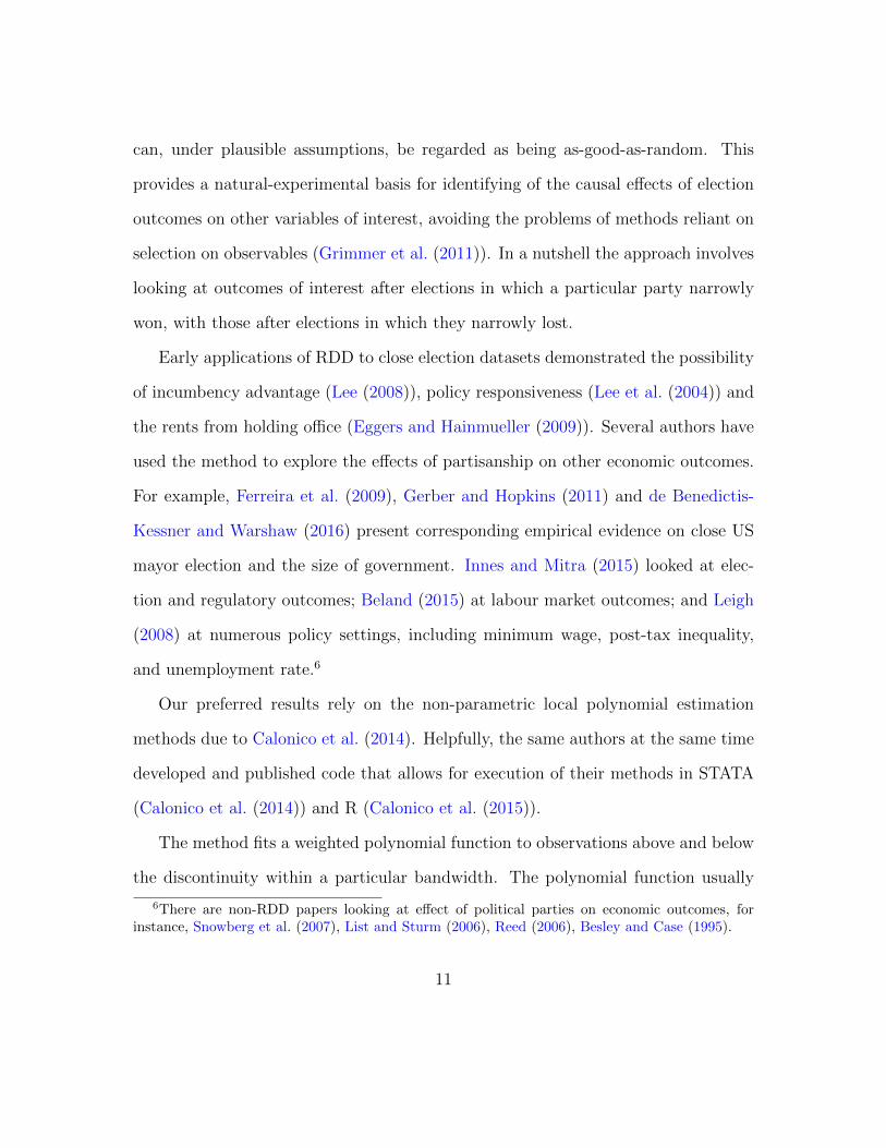
can, under plausible assumptions, be regarded as being as-good-as-random. This

provides a natural-experimental basis for identifying of the causal effects of election

outcomes on other variables of interest, avoiding the problems of methods reliant on

selection on observables (Grimmer et al. (2011)). In a nutshell the approach involves

looking at outcomes of interest after elections in which a particular party narrowly

won, with those after elections in which they narrowly lost.

Early applications of RDD to close election datasets demonstrated the possibility

of incumbency advantage (Lee (2008)), policy responsiveness (Lee et al. (2004)) and

the rents from holding office (Eggers and Hainmueller (2009)). Several authors have

used the method to explore the effects of partisanship on other economic outcomes.

For example, Ferreira et al. (2009), Gerber and Hopkins (2011) and de Benedictis-

Kessner and Warshaw (2016) present corresponding empirical evidence on close US

mayor election and the size of government. Innes and Mitra (2015) looked at elec-

tion and regulatory outcomes; Beland (2015) at labour market outcomes; and Leigh

(2008) at numerous policy settings, including minimum wage, post-tax inequality,

and unemployment rate.6

Our preferred results rely on the non-parametric local polynomial estimation

methods due to Calonico et al. (2014). Helpfully, the same authors at the same time

developed and published code that allows for execution of their methods in STATA

(Calonico et al. (2014)) and R (Calonico et al. (2015)).

The method fits a weighted polynomial function to observations above and below

the discontinuity within a particular bandwidth. The polynomial function usually

6There are non-RDD papers looking at effect of political parties on economic outcomes, forinstance, Snowberg et al. (2007), List and Sturm (2006), Reed (2006), Besley and Case (1995).

11

takes order 1 or 2, and the weights are determined endogenously, not by researcher

discretion, by a kernel function that performs the computation based on the distance

of observations from the discontinuity. Within the bandwidth, the closer the obser-

vation is to the discontinuity the more heavily it is weighted. An election with a

winning margin of 0.03% is given greater weight than an election won by 3%. This

implementation does not impose a parametric form of regression functions (Skovron

and Titiunik (2015)). Excluding the observations far away from the cut-off prevent

the distortion of the approximation near the cut-off (Gelman and Imbens (2014)).

The steps in estimation are as follows.

First, a bandwidth h is selected. The bandwidth is the width of the interval

around the discontinuity within which the local polynomial is fitted. Typically this

choice has been made arbitrarily, and for election-based studies has been set at 5% or

10% winning margins (de la Cuesta and Imai (2016), Erikson et al. (2015), Beland

(2015)). In choosing bandwidth the researcher faces a trade-off between bias and

variance.7 We follow the procedure developed in Calonico et al. (2014) for choosing

the optimal bandwidth - that which minimizes the asymptotic mean squared error

(MSE) of the regression discontinuity estimator, where MSE is the sum of the bias

squared and variance of the estimator. The choice of optimal bandwidth also means

that we avoid ad hoc decisions and the risk of (conscious or inadvertent!) specification

searching.

Second, a kernel function K(·) is chosen. The function assigns non-negative

7As observations fall further from the discontinuity - margin of victory is greater - the as-good-as-random assignment assumption becomes less palatable, introducing the risk of bias. A broaderbandwidth, however, means more data points.

12

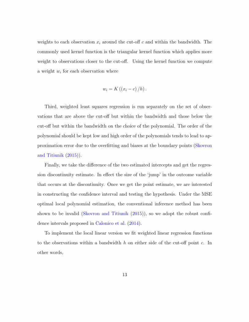
weights to each observation xi around the cut-off c and within the bandwidth. The

commonly used kernel function is the triangular kernel function which applies more

weight to observations closer to the cut-off. Using the kernel function we compute

a weight wi for each observation where

wi = K ((xi − c) /h) .

Third, weighted least squares regression is run separately on the set of obser-

vations that are above the cut-off but within the bandwidth and those below the

cut-off but within the bandwidth on the choice of the polynomial. The order of the

polynomial should be kept low and high order of the polynomials tends to lead to ap-

proximation error due to the overfitting and biases at the boundary points (Skovron

and Titiunik (2015)).

Finally, we take the difference of the two estimated intercepts and get the regres-

sion discontinuity estimate. In effect the size of the ‘jump’ in the outcome variable

that occurs at the discontinuity. Once we get the point estimate, we are interested

in constructing the confidence interval and testing the hypothesis. Under the MSE

optimal local polynomial estimation, the conventional inference method has been

shown to be invalid (Skovron and Titiunik (2015)), so we adopt the robust confi-

dence intervals proposed in Calonico et al. (2014).

To implement the local linear version we fit weighted linear regression functions

to the observations within a bandwidth h on either side of the cut-off point c. In

other words,

13

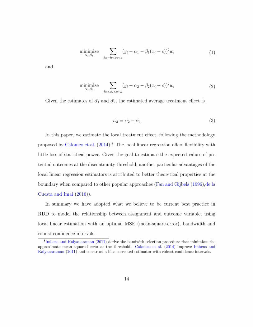
minimizeα1,β1

∑i:c−h<xi<c

(yi − α1 − β1(xi − c))2wi (1)

and

minimizeα2,β2

∑i:c<xi<c+h

(yi − α2 − β2(xi − c))2wi (2)

Given the estimates of α1 and α2, the estimated average treatment effect is

τrd = α2 − α1 (3)

In this paper, we estimate the local treatment effect, following the methodology

proposed by Calonico et al. (2014).8 The local linear regression offers flexibility with

little loss of statistical power. Given the goal to estimate the expected values of po-

tential outcomes at the discontinuity threshold, another particular advantages of the

local linear regression estimators is attributed to better theoretical properties at the

boundary when compared to other popular approaches (Fan and Gijbels (1996),de la

Cuesta and Imai (2016)).

In summary we have adopted what we believe to be current best practice in

RDD to model the relationship between assignment and outcome variable, using

local linear estimation with an optimal MSE (mean-square-error), bandwidth and

robust confidence intervals.

8Imbens and Kalyanaraman (2011) derive the bandwith selection procedure that minimizes theapproximate mean squared error at the threshold. Calonico et al. (2014) improve Imbens andKalyanaraman (2011) and construct a bias-corrected estimator with robust confidence intervals.

14

1.2.2 Study Setting

States are the primary subdivisions of the US and have a high degree of autonomy

in how they govern themselves. Each state possesses a number of important powers

including the operation of local government, regulating business, levying taxes and

spending tax revenues. The head of a state is called a Governor. He or she controls

the governmental budget, appoints many officials, and has a plethora or other powers.

Governors can veto bills and, in many cases, have the power of the line-item veto

on appropriation bills. In addition to hard authority, the governor can also bring

to bear significant ‘soft’ power through the authority given to him by his office. In

summary, governors are influential players in US politics.

A governor may run his or her state in a way that makes it more or less attractive

to a prospective international investor. In addition, in recent decades they have been

increasingly visible players on the international scene. External state-promotional

activity dates back to the 1970s (Fry (1998), Watson (1995)) and has focussed on

promoting trade and attracting inward investment. As regards FDI in particular,

states take the lead role in recruitment of inward investment, with the role of the

federal government much smaller. Many state-operated international offices and

governor-led overseas missions are set up to attract FDI (McMillan (2009)). US state

officials claim that the international trade and investment is the largest category of

state international engagement (Whatley (2003)). As a result, the governor of a state

acts as the chief economic ‘ambassador’ in appealing to prospective investors.

15

1.2.3 Data

We obtain data from several sources.

Our outcome variable of interest is FDI. State level FDI data is drawn from US

Bureau of Economic Analysis. We first obtain the total monetary amount of FDI

stock and the FDI stock in manufacturing sectors in each US State for each year

from 1977 to 2004. The FDI stock refers to the real book value of gross property,

plant, and equipment (PPE) of all nonbank affiliates. This includes the value of

buildings, structures, machinery, and equipment, etc., but excludes inventories and

intangible assets. It corresponds to the standard definition of FDI in the US. We are

interested in FDI flows, so we take the difference between the FDI measures in the

year governor was elected (elections almost always occur in November) and each of

the four years following where governor took the office respectively. So for example, if

the a governor wins a close election in November 2005 we take the difference between

FDI stock in 2005 with that stock in 2006, 2007, 2008 and 2009. This allows us to

answer four slightly different questions: How much ‘extra’ FDI does a governor of

a particular political persuasion attract in his first year in office, first two years in

office, etc. In most cases the fourth variant can be taken to approximate the extra

FDI across the whole term in office. In addition, taking changes in the outcome

variable (rather than working with levels) serves to increase the statistical efficiency

of our regression discontinuity design (Lee and Lemieux (2010)).

Table 1.1 presents summary statistics for FDI and other covariates. The mean

FDI stock per capita across the whole of the US is 2796 USD and the mean FDI

16

stock per capita in the manufacturing sector 921 USD.

The data on gubernatorial elections are obtained from two sources. The election

data from 1977 to 1990 is drawn from dataset Candidate and Constituency Statistics

of Elections in the United States, 1788-1990 (ICPSR 7757) from the Inter-university

Consortium for Political and Social Research. The remaining election data comes

from Dave Leip’s Atlas of U.S. Presidential Elections (Leip (2008)).

Gubernatorial elections usually take place in November and the governor elected

takes power in the following January. A governor’s term usually is four years.9 We

define the election margin to be the percentage of votes obtained by the Republican

candidate minus the percentage obtained by the Democrat. Following that conven-

tion the discontinuity is at zero (we can ignore third candidates). If the election

margin is positive (negative), the Republican (Democrat) has won.

Table 1.2 summarizes outcomes in the 361 elections in our sample. Of those

Republicans won 186, Democrats won 175 times. In terms of close elections we count

for the purpose of this summary table those with winning margins of 5% and 10%.

Within a 5% interval around the cut-off, we get 81 elections of which Republicans

won 42 times, Democrats won 39 times. Of the 157 elections within 10% of the

cut-off Republicans won in 80, Democrats in 77. So by each of these metrics the

sample is roughly balanced, no party seems systematically more likely to prevail

when result margins are narrow. If we look at the elections in terms of incumbents

and challengers, we can see that incumbents win more often. However, in the case of

close elections, the winning frequency of incumbents and challengers are balanced.

9The exceptions to this are New Hampshire and Vermont, where terms are two years. They donot feature in our dataset.

17

Incumbents won rough same number of times as challengers in 5% margins, while

challengers won slightly more times in 10% margins. The close-to-symmetric shape

of the barchart of density of winning margins in figure 1.1 is consistent with this.

Together these numbers suggest that there is no precise manipulation of selection into

the treatment, which would threaten the validity of the identification assumption on

which application of the RDD rests. To back-up this ‘eye-ball’ test, we will conduct

and present the results of more formal tests later.

To improve precision other control variables are included. In particular, we control

for state measures for population, percentage of the state workforce under union con-

tract, average hourly earnings in manufacturing, unemployment rate and education.

In addition, we add some state specific controls including farmland and urbanization.

Farmland is the percentage of each state’s total acreage that is farmland in year 2004

and urbanization refers to the percentage of population in urbanized areas and urban

clusters in the year 2000.

Data for the control variables are obtained from several sources. The labour-

related variables are from U.S. Bureau of Labour Statistics. Figures for educational

expenditures and urbanization are from U.S. Census Bureau. Farmland is from the

U.S. Department of Agriculture Economic Research Service.

18

1.3 Results

1.3.1 Main results

Table 1.3 and table 1.4 present main results on the causal impact of the election

of a Republican on (1) FDI per capita and (2) FDI in manufacturing per capita.

Significance levels are adjusted by robust inference methods proposed by Calonico

et al. (2014). The robust p-values are regarded as conservative, so the significance of

the results reported will also hold if we were to use conventional p-values. Standard

errors are clustered at state level.

Table 1.3 relates to FDI per capita. The top number in each column is the

estimated discontinuity - the additional FDI causally attributed to a Republican

win. In each panel, column (1) derives from estimates with no controls. Column

(2) includes a control for whether the election was associated with a change in ruling

party. Column (3) adds party change and other controls. The estimates are generally

not significant. The second panel identifies a positive and significant effect of a

Republican win on FDI inflow in the two year window following an election win,

but the value becomes smaller and significance is lost (even at 10%) once controls

are added. Overall the analysis reported in table 1.3 points to no discernible effect,

positive or negative, of a Republican governorship.

Table 1.4 reports the results of conducting the same exercise but specialized on

flows of FDI per capita into the manufacturing sectors. We find a significant positive

effect of a Republican governor on these flows, which can be interpreted causally.

19

The effect sustains whole term of governor. The results are relatively insensitive to

exclusion or inclusion of the control for party change or other controls.

Panel 1 implies that in his first year in office a Republican governor, other things

equal, attracts an additional 97.11 USD dollars of FDI in manufacturing per head

compared to his Democratic counterpart. In the first two years he attracts an addi-

tional 156.51 USD. In his first three years 262.88 USD. And in the full four years of

his term an additional 195.59 USD. Note that these are not ‘within year’ flows, but

rather the cumulative effect over four different time horizons. The state-level aver-

age FDI per capita in manufacturing in our sample is 920.82 USD so against that

benchmark, the growth in FDI stock in manufacturing activities is 21% higher under

a Republican governor during a four year term compared to a the counter-factual of

a Democratic governor.

Figure 1.2 and figure 1.3 plot the estimates RD estimates of the effects of a

Republican governorship on cumulative FDI per capita (Figure 1.2) and FDI in

manufacturing per capita (Figure 1.3) across each of the four time horizons. The

plotted estimates are based on our preferred specifications with all controls and the

confidence levels are presented at 90% and 95%.

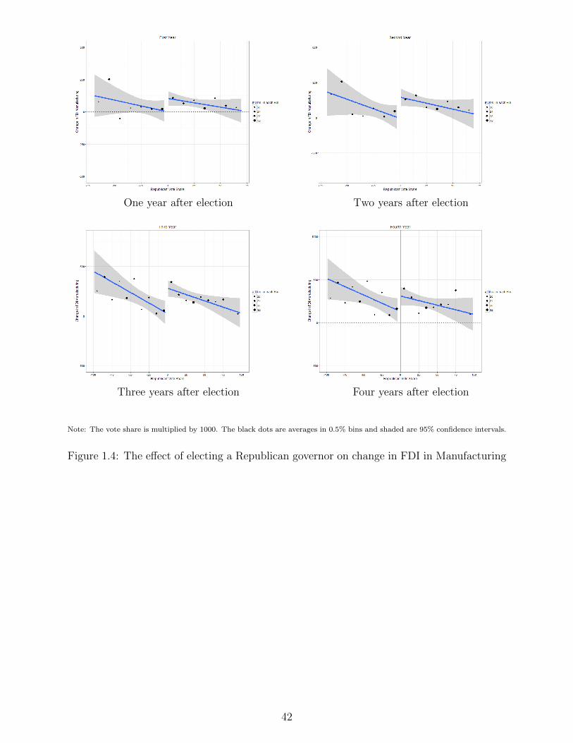
Figure 1.4 present the fitted curves either side of the discontinuity for each of the

four exercises (recall that each exercise refers to a different time horizon over which

the impact of the governorship on cumulative FDI is assessed). The ‘jump’ in the

vicinity of the discontinuity is the effect presented in the earlier tables, and it can be

seen here to be positive in each of the four panels. The size of each dot is determined

by the number of election data points in each winning margin bucket. While the

20

specifications reported are estimated over a wider interval, we can see comparatively

large dots in the immediate vicinity either side of the discontinuity, and that visually

there is a very apparent step up from those just to the left of the discontinuity to

those just to the right. While the data points further from the discontinuity are

included in the estimates, they carry correspondingly lower weight.

To summarize; (1) we find no evidence that the political affiliation of the state

governor has a causal impact on total FDI inflow. However, (2) there is a significant

(at 1%), positive and substantial effect of a Republican governorship on inflows of

manufacturing FDI, an effect that is sustained across the whole of the governor’s

term in office.

1.3.2 Validity

In this section, we challenge our study design by performing three validity checks.

A key assumption of RDD is the continuity assumption - that the only change

which occurs at the point of discontinuity is the shift in the treatment status.10 This

would be compromised if, for example, one party or the other were able to manipulate

the winning margin such as to be ‘just over the line’. In our setting, the violation of

the continuity assumption would require the eventual winner be able to predict vote

shares with extreme precision and then deploy necessary resources to win the close

elections. Existing evidence suggests that this is not a significant risk in our setting

10de la Cuesta and Imai (2016) distinguish the continuity assumption from the local randomizationassumption, where the latter one is more restricted. For the local randomization assumption to bemet, within a window of pre-specified size around the discontinuity threshold, whether or not anobservation receives the treatment is essentially randomly determined. de la Cuesta and Imai (2016)argue that the local randomization assumption is not required for the RD design to be valid.

21

(Eggers et al. (2015), de la Cuesta and Imai (2016)). However, the following validity

checks confirm that there is no evidence of such sorting behavior.

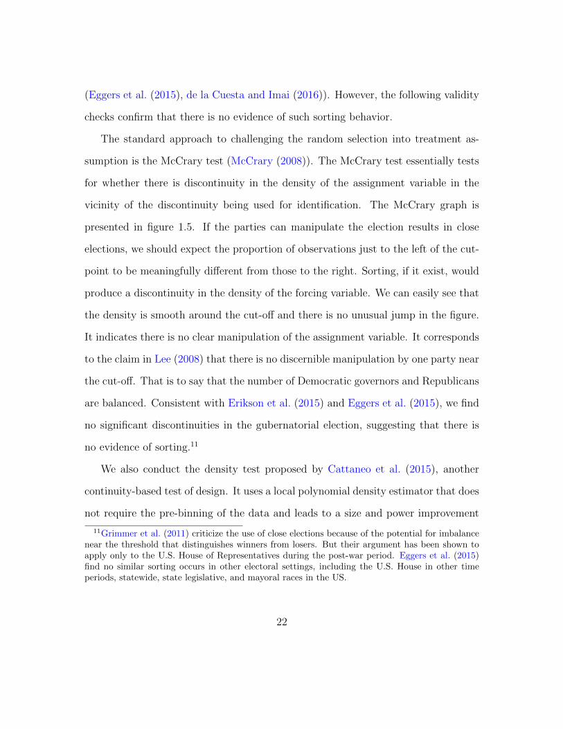
The standard approach to challenging the random selection into treatment as-

sumption is the McCrary test (McCrary (2008)). The McCrary test essentially tests

for whether there is discontinuity in the density of the assignment variable in the

vicinity of the discontinuity being used for identification. The McCrary graph is

presented in figure 1.5. If the parties can manipulate the election results in close

elections, we should expect the proportion of observations just to the left of the cut-

point to be meaningfully different from those to the right. Sorting, if it exist, would

produce a discontinuity in the density of the forcing variable. We can easily see that

the density is smooth around the cut-off and there is no unusual jump in the figure.

It indicates there is no clear manipulation of the assignment variable. It corresponds

to the claim in Lee (2008) that there is no discernible manipulation by one party near

the cut-off. That is to say that the number of Democratic governors and Republicans

are balanced. Consistent with Erikson et al. (2015) and Eggers et al. (2015), we find

no significant discontinuities in the gubernatorial election, suggesting that there is

no evidence of sorting.11

We also conduct the density test proposed by Cattaneo et al. (2015), another

continuity-based test of design. It uses a local polynomial density estimator that does

not require the pre-binning of the data and leads to a size and power improvement

11Grimmer et al. (2011) criticize the use of close elections because of the potential for imbalancenear the threshold that distinguishes winners from losers. But their argument has been shown toapply only to the U.S. House of Representatives during the post-war period. Eggers et al. (2015)find no similar sorting occurs in other electoral settings, including the U.S. House in other timeperiods, statewide, state legislative, and mayoral races in the US.

22

(Skovron and Titiunik (2015)). We are able to reject the null hypothesis that the

density is discontinuous at the cut-off with an associated P-value of 0.4496.

To further examine whether the key identification assumption of the RD design

is credible, we conduct placebo tests on a number of covariates. In particular, we

perform the estimation on the covariates following the same methodology, and the

results are presented in table 1.5. We find no significance, indicating that the covari-

ates are balanced.12 Results show that party affiliation of the governor has no effect

on these variables.

1.3.3 Methodological robustness

In the main results section we explored the robustness of our main estimates to

exclusion and inclusion of a variety of state-level controls. In this section, we perform

sensitivity tests to examine the robustness of our RDD results as they apply to FDI

in manufacturing to changes in modelling assumptions.13

Senate/House & President

In our preferred specification, we add state and time-varying characteristics including

state population, percentage of the state workforce under union contract, average

hourly earnings in manufacturing, unemployment rate, education expenses, farmland

12de la Cuesta and Imai (2016) argue that under the continuity assumption, observations oneither side of the discontinuity threshold can systematically differ from each other in many aspects,even by a large magnitude. The imbalance of barely-winners and barely-losers near the thresholddoes not necessarily invalidate the application of the RDD. Nonetheless we find the covariates arebalanced in our setting and the continuity assumption holds.

13We conducted similar exercises on the aggregate FDI data (that tested the robustness of theresults in table 1.3) and obtain similar results. In other words the non-significance result in thatcase proves robust. We do not report these in detail here.

23

and urbanization in order to control for possible confounding factors that might

influence the results.

To better isolate the impact of the gubernatorial election, we include more factors

that may play roles in shaping foreign economic policies. In addition to state gover-

nor, state legislatures are also regarded powerful on international issues (McMillan

(2009)). In table 1.6 we include the variables indicating which party controls the

house and which controls the senate. Also, the party holds office at national level

matters for setting the economic climate. In table 1.6 we control that the variables in-

dicating which party the president belongs to. The results are robust to the inclusion

of dummy variables for having Republicans control the state senate, for Republicans

controlling the state house, and for the president being a Republican.

Bandwidth

For our preferred estimates we adopted a optimal bandwidth following Calonico et al.

(2014). The optimal bandwidth selected by the method varies between about 7%

and 10% across the specifications. This is similar to the bandwidth chosen (usually

arbitrarily) in other applications of RDD methods to close elections.14 Nonetheless,

as robustness checks we re-run each regression imposing first a 5% and then a 10%

bandwidth. The results of these exercises are presented in table 1.7. The estimates

retain sign and significance and are similar in value to those from the preferred

specifications in table 1.4.

14Our bandwidth is close to Caughey et al. (2016) who study the effect of guernatorial electionoutcomes on policy liberalism and de Benedictis-Kessner and Warshaw (2016) who use similarbandwidth when examining how the size of government reacts to outcomes of US mayoral election.Our bandwidth is tighter than, for example, Klasnja and Titiunik (2014).

24

Order of polynomial

In our base specification we fitted the data linearly on either side of the discontinu-

ity. This is the preferred approach because Gelman and Imbens (2014) argue that

estimators for causal effects based on high order (third, fourth, or higher) polynomi-

als can be misleading in the RDD setting. Gelman and Imbens (2014) recommend

instead use estimators based on local linear or quadratic polynomials.

In table 1.8 we report the results of repeating the exercise but fitting a second-

order polynomial. Again we can see that the size of the estimated effects are little

disturbed, and in all cases the sign and significance of the effect is sustained.

Outliers

To allay concerns that the result is being driven by a small number of extreme ob-

servations we perform outlier analysis by winsorizing data at 99% and 95% level.

Winsorization is the statistical transformation of the data by limiting extreme val-

ues in the data to reduce the effect of (possibly spurious) outliers (winsorization is

widely used by economists (Alesina et al. (2015), Dick and Lehnert (2010)). A 99%

winsorization, for example, would see all data below the 1st percentile set to the 1st

percentile, and data above the 99th percentile set to the 99th percentile. Winsoriza-

tion methods are usually more robust to outliers, although there are alternatives,

such as trimming, that will achieve a similar effect. One advantage of winsorization

is that the transformation limits the impact of outliers, without losing observations.

The results are presented in the table 1.9. The results are little disturbed by the

winsorization suggesting that they are not overly driven by a few extreme-valued

25

outliers.

Alternative denominator for dependent variable

Our central analysis took as dependent variable FDI per capita as out measure of

FDI intensity. An alternative and equally sensible approach would have been to work

with FDI per unit of percentage of state level GSP. To confirm that this would not

significantly have disturbed conclusions we re-estimate our preferred specification on

that basis. The results of this exercise are reported in table 1.10.

In this version, a Republican governor - compared to the benchmark of a Demo-

crat - causes a 12% increase in FDI stock in manufacturing as a percentage of the

gross state product after one year and an increase of 27% over the four-year term in

office. These are qualitatively similar to our main results, though somewhat larger

in size.

1.4 Possible Channels

Economic theory suggests a large variety of potential mechanisms that relate political

parties and attraction of FDI. Political parties can influence the location choices of

multinationals in both direct and indirect ways. On one hand, state governments can

influence the foreign investors directly by offering investment incentives of various

kinds, like tax credits, cheap loans, access to foreign trade zones, and a variety of

subsidies. On the other hand, the attraction policy can be indirect when a state’s

general economic development policies are shaped by political choices concerning

26

infrastructure development, investment in education, and labor-market regulation

policies. But the question of exactly how and to what degree each targeting policies

matter is still largely unresolved (Halvorsen and Jakobsen (2013)).

The literature on FDI determinants documents a number of factors multinational

companies consider. The factors may include, market size and growth potential

(Resmini (2000)), industry clustering (Wheeler and Mody (1992)), labor market

flexibility and financial depth (Yu and Walsh (2010)), infrastructure, institutional

quality, tax level, political risk (Dunning (1998)). But the relative importance of

those factors to the international investors of these different traits is complex. The

multinationals with long time horizons and multifaceted location motives, rarely

count solely on any single incentive offered by states (Halvorsen and Jakobsen (2013).

It is outside the scope of our analysis to investigate the exact mechanisms of

impact of political parties on FDI. Foreign investors’ decision could be influenced by

various economic policies adopted by political parties in office. We take advantage

of the RDD method by uncovering the net impact of those implemented economic

policies.

1.5 Conclusion

Foreign investment plays a crucial role in the American - and other - economies.

But how influential is the type of government in a place in determining the levels or

patterns of inward investment?

In this paper, we present what we believe to be the first empirical investigation

27

of a causal link from political partisanship to FDI. As such we provide a further

empirical point-of-connection between political and economic outcomes, with a di-

rection of effect. To obtain plausibly exogenous assignment of treatment (political

party in power) we use a regression discontinuity design, exploiting the discontinuity

generated by the first-past-the-post election system.

The evidence points to Republican governors causing a substantial and sustained

upward bump in foreign investment into manufacturing activities, when compared to

their Democratic counterparts. However, we find no evidence one way or the other on

total FDI flows, although those effects are much less precisely estimated. Rather than

study particular mechanisms, an advantage of the RDD approach is that it allows

us to be agnostic regarding mechanism(s). It seems likely that Republicans do some

things that are attractive to investors, while Democrats may do other things, and

the analysis here estimates the net effect of those interventions when added together.

This line of research could fruitfully be taken forward in different ways. One

would be to explore the partisan effects on more finely classified activities - which

types of economic activity are more or less sensitive to political events than others?

A second is to explore the role of left- and right-leaning governments in settings other

than the US, with alternative political, social and economic landscapes.

28

Table 1.1: Summary Statistics

Mean Std. Dev Min Max(1) (2) (3) (4)

FDI Stock per Capita 2795.70 4972.94 71.77 47463.41

FDI Stock per Capita in Manufacturing 920.82 1017.17 16.61 8322.05

FDI Stock / GSP 0.112 0.143 0.009 1.844

FDI Stock in Manufacturing / GSP 0.041 0.036 0.002 0.275

Population 4986858 5483532 397363 35842038

Union 15.741 7.142 2.8 38.3

Wage 13.454 1.740 9.589 21.329

Unemployment 2.924 0.948 1.081 12.166

Education Expense 32.889 6.268 15.957 50.201

Farm Land 41 24.3 1 93

Urbanization 71.70 14.76 38.2 94.4

Note: Union: percentage of the state workforce under union contract; Wage: average hourly earnings in manufacturing;Education expense: total state expenditure on education as a percentage of total government expenditure; Farm Land: thepercentage of each state’s total acreage that is farmland in 2004; Urbanization: percentage of population in urbanized areasand urban clusters in 2000.Source: FDI-related variables are from U.S. Bureau of Economic Analysis;labour-related variables are from U.S. Bureau of labourstatistics; Population, Education and Urbanization variable is from U.S. Census Bureau; Farmland is from U.S. Department ofAgriculture Economic Research Service.

29

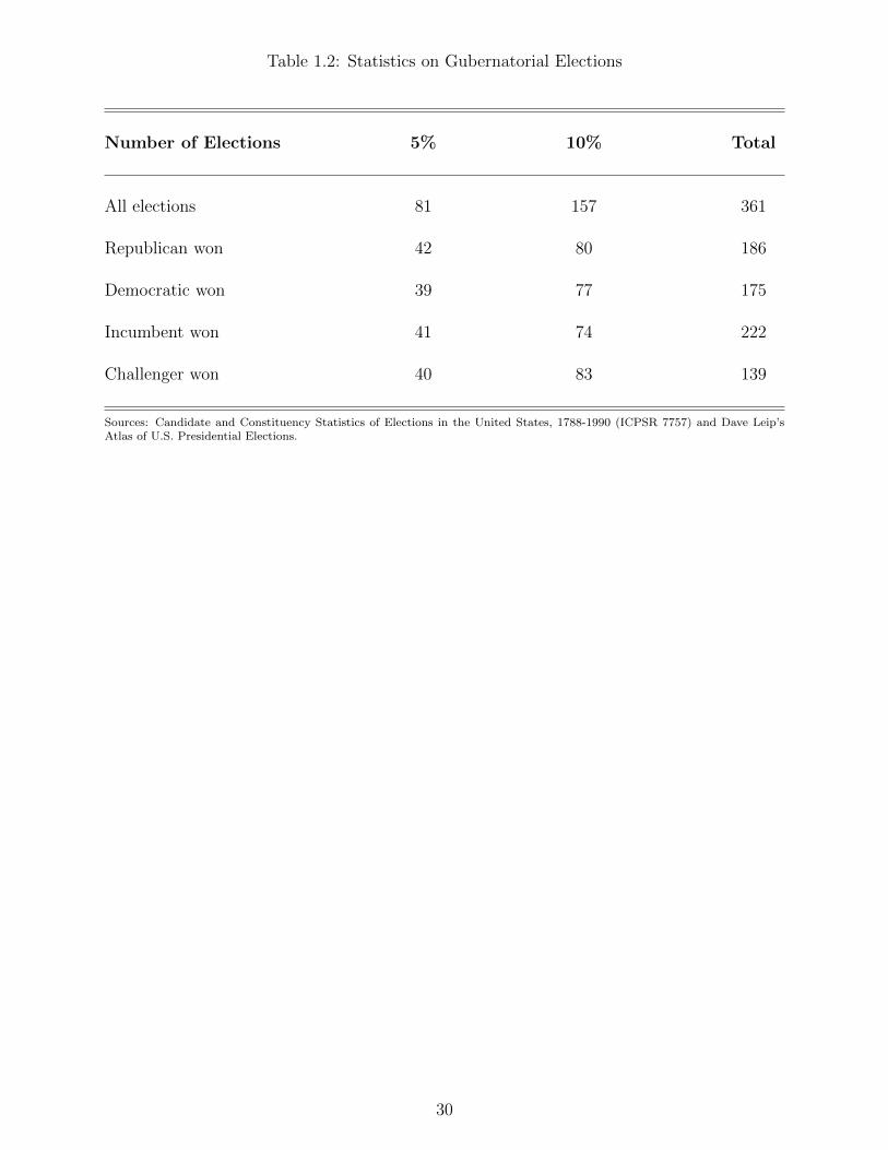
Table 1.2: Statistics on Gubernatorial Elections

Number of Elections 5% 10% Total

All elections 81 157 361

Republican won 42 80 186

Democratic won 39 77 175

Incumbent won 41 74 222

Challenger won 40 83 139

Sources: Candidate and Constituency Statistics of Elections in the United States, 1788-1990 (ICPSR 7757) and Dave Leip’sAtlas of U.S. Presidential Elections.

30

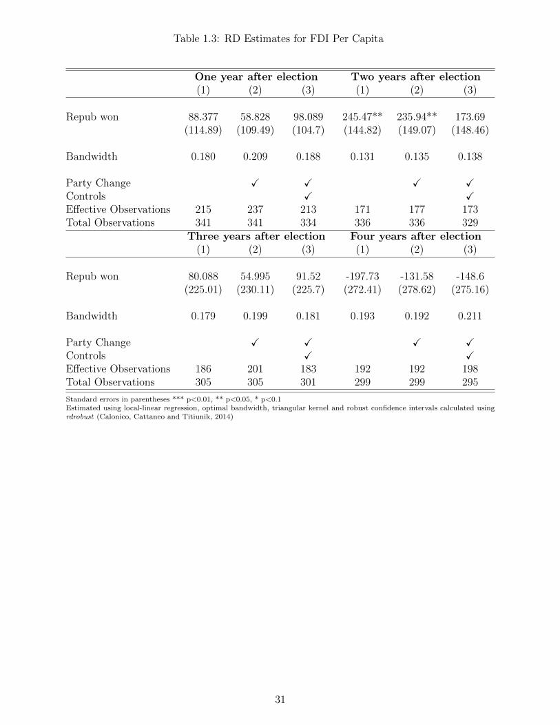
Table 1.3: RD Estimates for FDI Per Capita

One year after election Two years after election(1) (2) (3) (1) (2) (3)

Repub won 88.377 58.828 98.089 245.47** 235.94** 173.69(114.89) (109.49) (104.7) (144.82) (149.07) (148.46)

Bandwidth 0.180 0.209 0.188 0.131 0.135 0.138

Party Change X X X XControls X XEffective Observations 215 237 213 171 177 173Total Observations 341 341 334 336 336 329

Three years after election Four years after election(1) (2) (3) (1) (2) (3)

Repub won 80.088 54.995 91.52 -197.73 -131.58 -148.6(225.01) (230.11) (225.7) (272.41) (278.62) (275.16)

Bandwidth 0.179 0.199 0.181 0.193 0.192 0.211


Standard errors in parentheses *** p<0.01, ** p<0.05, * p<0.1Estimated using local-linear regression, optimal bandwidth, triangular kernel and robust confidence intervals calculated usingrdrobust (Calonico, Cattaneo and Titiunik, 2014)

31

Table 1.4: RD Estimates for FDI Manufacturing Per Capita

One year after election Two years after election(1) (2) (3) (1) (2) (3)

Repub won 103.04*** 102.84*** 97.107*** 177.56*** 176.31*** 156.51***(38.706) (38.193) (32.027) (59.49) (59.394) (44.857)

Bandwidth 0.072 0.074 0.075 0.076 0.077 0.081


Three years after election Four years after election(1) (2) (3) (1) (2) (3)

Repub won 240.06*** 242.18*** 262.88*** 145.97** 144.53** 195.59***(59.21) (59.034) (53.244) (66.121) (65.789) (60.975)

Bandwidth 0.110 0.110 0.084 0.115 0.115 0.102



32

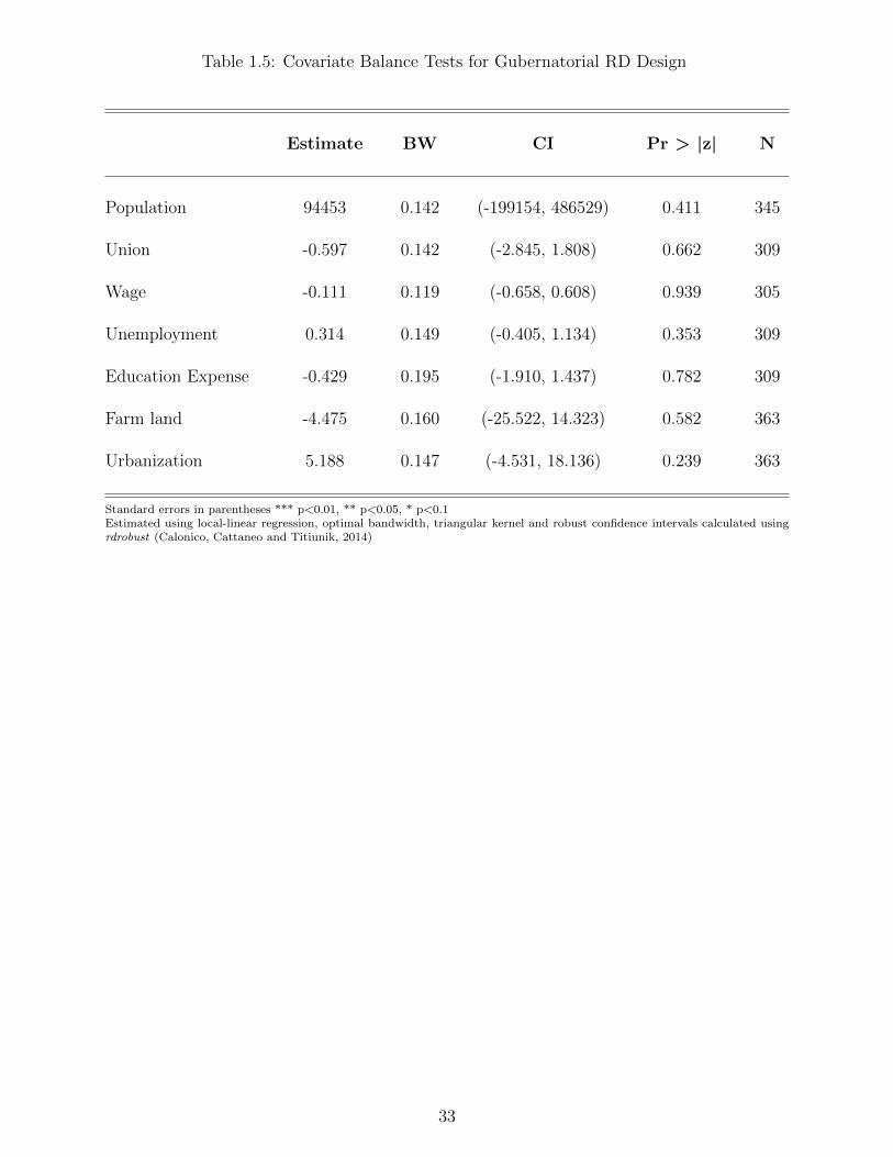
Table 1.5: Covariate Balance Tests for Gubernatorial RD Design

Estimate BW CI Pr > |z| N

Population 94453 0.142 (-199154, 486529) 0.411 345

Union -0.597 0.142 (-2.845, 1.808) 0.662 309

Wage -0.111 0.119 (-0.658, 0.608) 0.939 305

Unemployment 0.314 0.149 (-0.405, 1.134) 0.353 309

Education Expense -0.429 0.195 (-1.910, 1.437) 0.782 309

Farm land -4.475 0.160 (-25.522, 14.323) 0.582 363

Urbanization 5.188 0.147 (-4.531, 18.136) 0.239 363


33

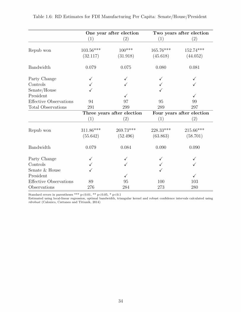
Table 1.6: RD Estimates for FDI Manufacturing Per Capita: Senate/House/President

One year after election Two years after election(1) (2) (1) (2)

Repub won 103.56*** 100*** 165.76*** 152.74***(32.117) (31.918) (45.618) (44.052)

Bandwidth 0.079 0.075 0.080 0.081

Party Change X X X XControls X X X XSenate/House X XPresident X XEffective Observations 94 97 95 99Total Observations 291 299 289 297

Three years after election Four years after election(1) (2) (1) (2)

Repub won 311.86*** 269.73*** 228.33*** 215.66***(55.642) (52.496) (63.863) (58.701)

Bandwidth 0.079 0.084 0.090 0.090

Party Change X X X XControls X X X XSenate & House X XPresident X XEffective Observations 89 95 100 103Observations 276 284 273 280


34

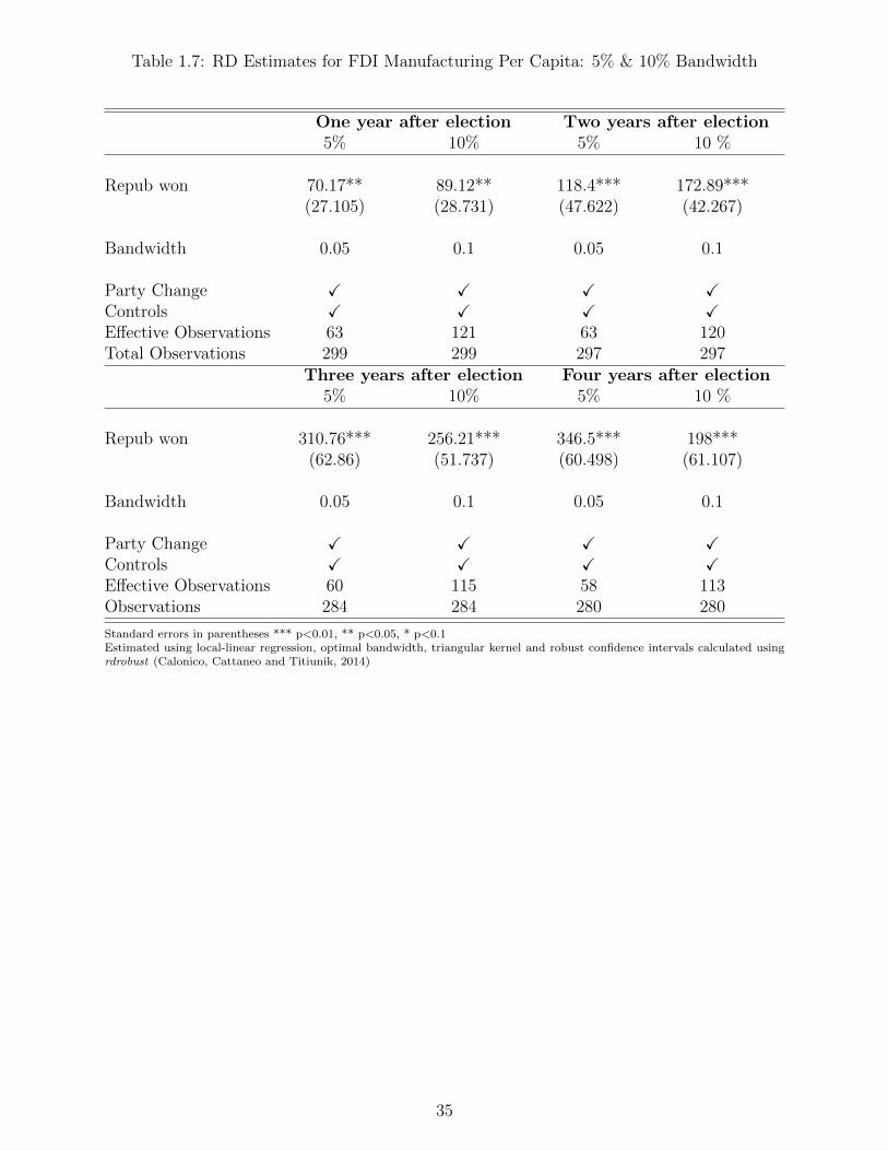
Table 1.7: RD Estimates for FDI Manufacturing Per Capita: 5% & 10% Bandwidth

One year after election Two years after election5% 10% 5% 10 %

Repub won 70.17** 89.12** 118.4*** 172.89***(27.105) (28.731) (47.622) (42.267)

Bandwidth 0.05 0.1 0.05 0.1

Party Change X X X XControls X X X XEffective Observations 63 121 63 120Total Observations 299 299 297 297

Three years after election Four years after election5% 10% 5% 10 %

Repub won 310.76*** 256.21*** 346.5*** 198***(62.86) (51.737) (60.498) (61.107)

Bandwidth 0.05 0.1 0.05 0.1

Party Change X X X XControls X X X XEffective Observations 60 115 58 113Observations 284 284 280 280


35

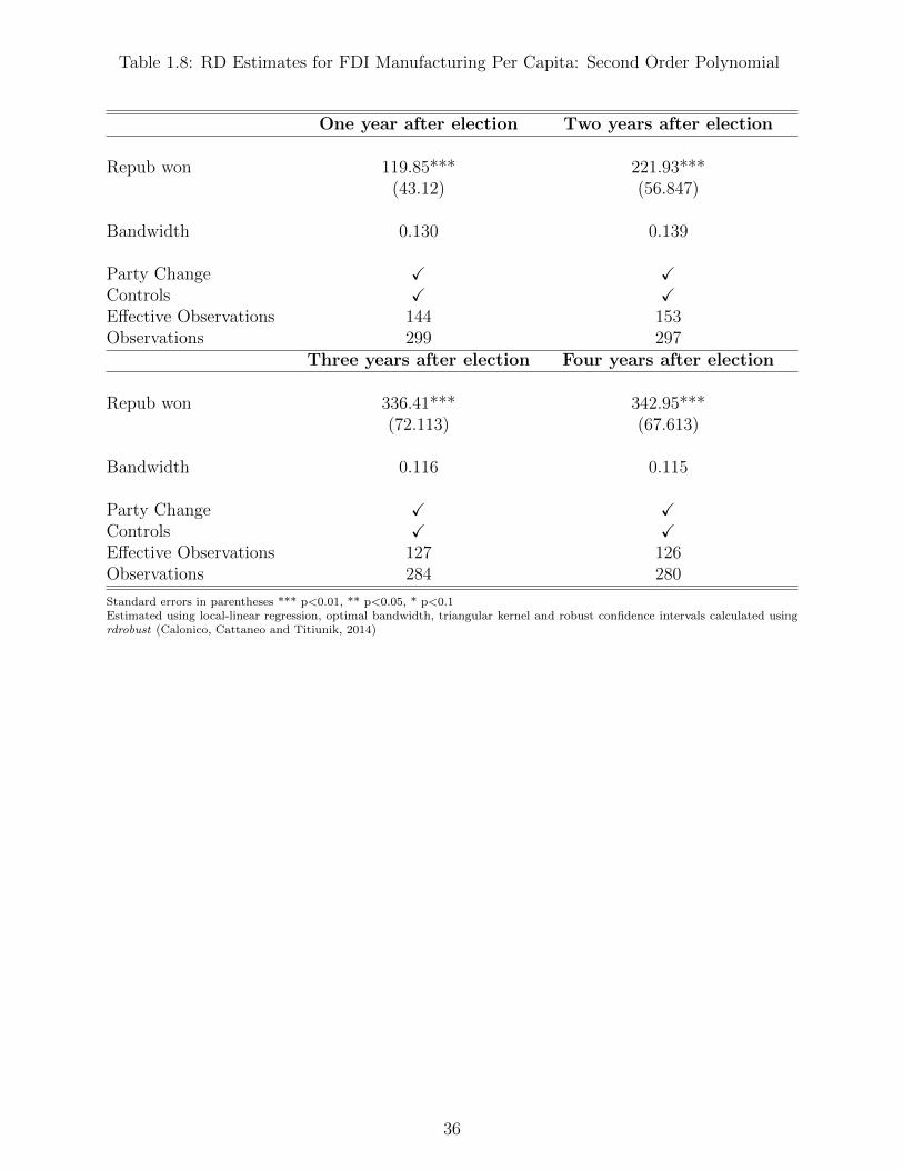
Table 1.8: RD Estimates for FDI Manufacturing Per Capita: Second Order Polynomial

One year after election Two years after election

Repub won 119.85*** 221.93***(43.12) (56.847)

Bandwidth 0.130 0.139

Party Change X XControls X XEffective Observations 144 153Observations 299 297

Three years after election Four years after election

Repub won 336.41*** 342.95***(72.113) (67.613)




36

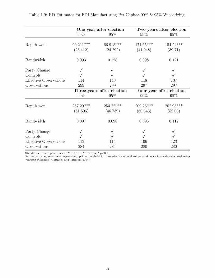
Table 1.9: RD Estimates for FDI Manufacturing Per Capita: 99% & 95% Winsorizing

One year after election Two years after election99% 95% 99% 95%

Repub won 90.211*** 66.918*** 171.65*** 154.24***(26.412) (24.292) (41.948) (39.71)

Bandwidth 0.093 0.128 0.098 0.121


Three years after election Four year after election99% 95% 99% 95%

Repub won 257.29*** 254.22*** 209.26*** 202.95***(51.596) (46.739) (60.343) (52.03)

Bandwidth 0.097 0.098 0.093 0.112



37

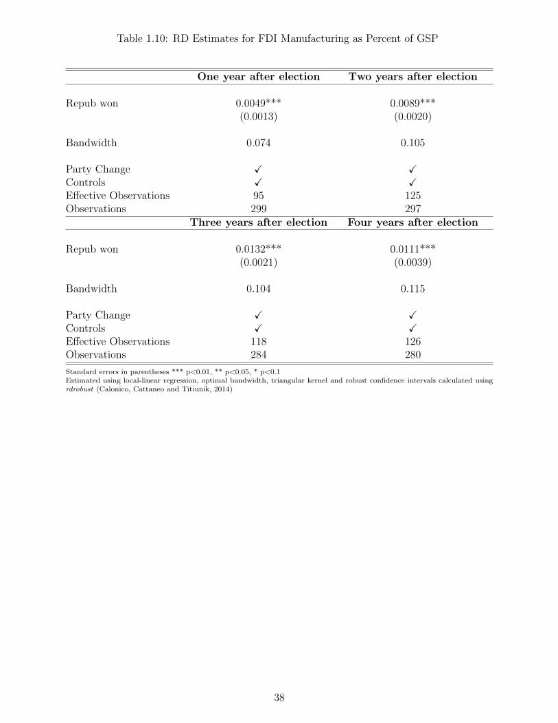
Table 1.10: RD Estimates for FDI Manufacturing as Percent of GSP


Repub won 0.0049*** 0.0089***(0.0013) (0.0020)




Repub won 0.0132*** 0.0111***(0.0021) (0.0039)




38

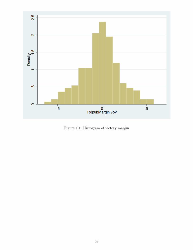
Figure 1.1: Histogram of victory margin

39

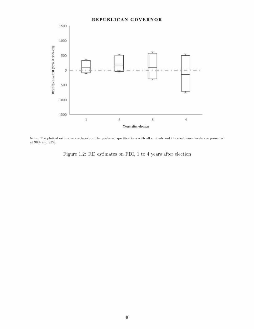
Note: The plotted estimates are based on the preferred specifications with all controls and the confidence levels are presentedat 90% and 95%.

Figure 1.2: RD estimates on FDI, 1 to 4 years after election

40

Note: The plotted estimates are based on the preferred specifications with all controls and the confidence levels are presentedat 90% and 95%.

Figure 1.3: RD estimates on FDI Manufacturing, 1 to 4 years after election

41



Note: The vote share is multiplied by 1000. The black dots are averages in 0.5% bins and shaded are 95% confidence intervals.

Figure 1.4: The effect of electing a Republican governor on change in FDI in Manufacturing

42

Figure 1.5: McCrary density of victory margin

43

Chapter 2

Commodity Price Shocks,

Institutions and Windows of

Opportunity for Structural Reform

2.1 Introduction

Finding a window of opportunity to conduct economic reform is one of the funda-

mental aims in political economy. Economic reform is difficult to implement, even

when we considered those that are efficiency-enhancing. Often times, we witness

reforms that are postponed or adopted after long delays, because reforms are rarely

being Pareto improvement, resulting in winners and losers. Unequal distributions

between benefits and costs exist both economically and politically, underlining the

non-neutrality feature of reform (Fernandez and Rodrik (1991)). The large distri-

44

butional shifts of economic reform raise the stakes for every citizen in the political

process, thus the state plays an important role in shaping the regulatory environment

and in promoting economic reform.

Two important questions remain unanswered in this field. First, does output

contraction induce reform? Does crisis shape the window of reform? The anticipated

effect of output on reform hinges on two countervailing factors. On one hand, some

evidence shows that crisis promotes reform due to the high cost of inaction and low

political cost (Alesina et al. (2006)). On the other hand, crisis reduces the resources

available to compensate losers, and thus deters reform from occurring (Bonfiglioli

and Gancia (2015)). Furthermore, large negative economic shocks could radically

change one’s belief on the current policy and in turn, promote reforms. Meanwhile

negative shocks raise the uncertainty and disagreement on the future economy and

may even lead to political gridlock (Abiad and Mody (2005)). The net effect of

economic shocks on reforms depend on the respective magnitudes of the effects.

Second, how do institutions decide when to conduct reforms? There are signif-

icant findings in the literature that emphasize the role of states and suggest that

political freedom and economic freedom go hand in hand (Persson and Tabellini

(2006)). Theoretically, democratic regimes implement more reforms if reforms create

more winners than losers. Indeed, democratic regimes make decisions within a com-

plex interaction between shifting voter preferences, strategic lobbying, and special

interest politics (Grossman and Helpman (2001)). Democratic regimes could lead to

fewer reforms if the electoral system creates a pivotal voter with veto power. The

uncertainty about the impact of economic reforms at the individual level could also

45

lead to votes against reforms even if a majority of them would benefit from the re-

form. Moreover, if we turn to look back to the reforms in East Asian countries, many

successful reforms were conducted in autocratic countries such as, South Korea and

Singapore. The evidence is still mixed and far from reaching a conclusion.

Despite the growing attention of both economists and policy makers on the topic,

little effort has been devoted to studying the effect of economic shocks on the adoption

of structural reforms. This paper analyzes the relationship between economic shocks

and structural reforms using unique data in 111 countries from 1962 to 2005. Previous

research is limited to case studies, the use of pre-existing data sources that cover

a relatively narrow set of reforms and countries. This paper addresses this issue

by using an expanded dataset on structural reform that includes many countries

across broader time-frame. Additionally, the economic literature ignores the fact

that national income is endogenous to economic reform and overwhelmingly fails to

find a causal effect between economic conditions and economic reform. This paper

addresses this issue by using the exogenous variation in the international price of

large commodity goods to generate the exogenous change in national income.

In the paper, we separately examine two types of structural reforms, namely,

reforms in financial market sector and reforms in the product market sector. Product

market sector reform is different from financial market sector reform in a number of

ways. Due to the nature of the market structure of the product market, the cost of

product market reform tends to concentrate on a few players. Thus, the target groups

who lose from the reform are often easy to identified and get compensated. It is often

not the case in the financial market. In addition, the impact of interest groups may be

46

amplified by several institutional factors, when industry representatives participate

in regulatory decisions in product markets (Høj et al. (2006), Faccio (2006)).

This paper contributes to the literature in two ways. First, we take advantage

of the changes in the international price of the principal commodity of a country

as exogenous sources of income fluctuation to identify the effect of national income

on reform. Secondly, this paper aims to investigate how economic shocks affect the

windows of reform under different institutional regimes. The findings in this paper

suggest that the reforms in autocratic countries are heavily affected by national

income shocks while it is not the case in democratic countries. In addition, the

product market reforms and the financial reforms tend to respond differently to the

economic shocks. Positive economic shocks promote product market reforms but

deter the financial reforms. The results are robust to a variety of robustness checks.

The paper proceeds as follows. Section 2 highlights the related literature. Section

3 describes the data. Section 4 illustrate the empirical methodology. Section 5 reports

our results and Section 6 concludes.

2.2 Literature Review

The political economy of reform has been documented both theoretically and em-

pirically. Theoretically, Fernandez and Rodrik (1991) look at the reform decisions

regarding democratic voting mechanisms and propose that the source of preventing

reforms is uncertainty regarding the distribution of gains and losses from the reform.

In particular, there is a bias toward the status quo whenever the individual win-

47

ners and losers from reform cannot be identified in advance. While on the empirical

side, Giuliano et al. (2013) find that an increase in the quality of democratic insti-

tutions has a positive and significant impact on the adoption of economic reforms.

Also, Alesina et al. (2006) find that reforms tend to follow periods of inflationary

and budgetary crisis, when new governments take office and when governments are

strong.

Concerning the timing of reforms, Ranciere and Tornell (2016) is in favor of the

hypothesis that crises facilitate economic reforms. Specifically, they present a model

where rent-seeking leads to economic decline, which, in turn, will make a future

reform inevitable when times will already be bad enough. Furthermore, they use

the case of trade liberalization as a prime example of structural reform to show

that reforms are induced by severe crises. In addition, Tommasi and Velasco (1996)

suggest that structural reforms tend to occur in crises rather than during prosperous

times based on the experiences of developing countries with market-oriented reforms.

On the other hand, Mian et al. (2014) show that banking, currency, inflation, or

debt crises lead to greater ideological polarization in society, greater fractionalization

of the legislative body, and a decrease in the size of the working majority of the ruling

coalition. The raising political polarization could weaken incumbent governments

and hinder the adoption of the financial reforms.

Moreover, Drazen and Easterly (2001) find mixed evidence of crisis-induced re-

forms. In particular, they find that the reforms are more likely to be conducted

following episodes of high inflation rate and black market premium, but no evidence

show that high current account deficit, high budget deficit, and negative per capita

48

growth rate is correlated with reforms.

The effectiveness of reforms is another strand of related literature. Several em-

pirical papers have looked at the outcomes of reforms. Prati et al. (2013) suggest

that both real sector and financial sector reforms are promoting economic growth,

but the positive effect of reform is influenced by a country’s constraints on the au-

thority of the executive power and by its distance from the technological frontier.

Even though, the evaluation of the reforms is beyond the scope of this paper, the

systematic empirical work in this field conveys an important message that reforms

are mostly complicated issues, and thus the adoption of reforms could differ in timing

and institutions.

The literature on economic shocks from commodity prices is also rich. The ef-

fect of economic shocks on political-economy outcomes like conflicts and democratic

change are widely investigated. Bruckner and Ciccone (2010) examine the effect of

economic conditions on civil war, and find a robust effect of commodity price down-

turns on the outbreak of civil wars, and they also find that Sub-Saharan countries

are more likely to engage in civil wars following economic downturns in their main

OECD export destinations.

Caselli and Tesei (2016) document the effect of natural resource windfalls on

political regimes. Their results indicate that natural resource windfalls have no

effect on the political system when they occur in democracies, while windfalls have

significant political consequences in autocracies. In deeply entrenched autocracies,

the effect of windfalls on politics is little, while in moderately entrenched autocracies,

the effect is significantly larger.

49

Bruckner et al. (2012) look at the oil price shock on the democratic change.

They find that countries with greater net oil exports over GDP see improvements in

democratic institutions following upturns in international oil prices. However, Burke

and Leigh (2010) use commodity price changes as instruments for income changes and

find insignificant effects of commodity-driven income changes on political regimes.

Numerous paper attempts to understand the determinants of structural reform

and how various economic conditions affect the likelihood of the adoption of reforms,

few of them establish a causal effect, which is where we want to fill the gap. Moreover,

the role of the interactions of institutions has received little attention when analyzing

the impact of economic conditions. Institutions play a significant role in economic

development (Acemoglu et al. (2001)). In fact, the political nature of an institutional

equilibrium that makes it very difficult to reform economic institutions (Acemoglu

et al. (2008), Acemoglu and Robinson (2008)). In this paper, we introduced the role

of institutions to analyze the timing of structural reform facing economic shocks.

2.3 Data

In this section, the data used in this paper is described and the data is obtained from

different sources. The sample period is from 1962 to 2005.

2.3.1 Data on reforms

The data on reforms comes from a completely new and extensive dataset, compiled

by the Research Department of the International Monetary Fund (IMF), describing

50

the degree of regulation for a sample of 150 industrial and developing countries. Prati

et al. (2013) describes all data sources of the reform indicators and full details of the

construction of the indicators.

Reform is usually defined as liberalization of markets and changes in the regula-

tory environment (Bonfiglioli and Gancia (2015), Giuliano et al. (2013), Høj et al.

(2006)). The following paragraphs present brief definitions and construction of the

reform indicators used in this paper. Reform indicators cover both financial and real

sectors. Financial sector reform indicators include reforms pertaining to domestic

financial markets, while real sector structural reform indicators include measures of

product markets, including telecommunication and electricity markets. The indi-

cators are constructed such that, firstly, both sectors contains different sub-indices

summarizing different dimensions of the regulatory environment in each sector. Sec-

ondly, the sub-indices are then aggregated into indices and normalized between 0

and 1 and the higher values represent greater degree of liberalization.

The measures of financial sector reforms are mainly for the domestic financial

sector. The domestic financial sector liberalization indicator in turn includes mea-

sures of regulation indicators of banking sector and securities markets. The banking

system index contains (1) credit controls, such as directed credit and subsidized lend-

ing, (2) interest rate controls, such as floors or ceilings, (3) competition restrictions,

such as limits on branches and entry barriers in the banking market, including li-

censing requirements or limits on foreign banks), (4) public ownership of banks. (5)

quality of banking supervision and regulation, including the power and independence

of bank supervisors, the adoption of Basel capital standards, and the presence of a

51

framework for bank inspections.

The security markets index captures the quality of the market framework, includ-

ing the degree of legal restrictions on the development of domestic bonds and equity

markets as well as the existence of independent regulators Turning to the real sector,

the product market indicator covers the degree of liberalization in the telecommuni-

cation and electricity markets, including the extent of competition in the provision

of these services, the presence of an independent regulatory authority, and degree of

privatization.

We use the variation in the absolute degree of economic liberalization within each

sector to measure the reform in the corresponding sector across countries and over

time. To be noted, the differences in the value of the indices across sectors do not

indicate a precise quantitative measure of whether one sector is more liberalized than

another due to the different methodology used to construct each index. A positive

difference between the index in the financial sector and the real sector does not

necessarily mean that the financial sector is more liberalized than the real sector.

2.3.2 Data on commodity prices

To construct a country level economic shock based on commodity price, we follow

the method used in Caselli and Tesei (2016). A country’s principal commodity is

identified as the commodity that is ranked first by its value of exports in the largest

number of years. Then the principal commodity is matched with the corresponding

world prices. The commodities include both agricultural and mineral commodities.

The principal commodity export shares and prices data are from UN Comtrade data

52

set and IMF IFS data set. The detailed data sources and construction are well-

documented in Caselli and Tesei (2016).

2.3.3 Data on institutions

Institutions are measured using the standard, well-established measure of democracy

taken from the Polity IV database, which measures the longitudinal patterns of the

political regime characteristics and transitions. The data on institutions is based on

the Polity2 variable in the Polity IV database. The Polity2 variable captures the

electoral rules and openness of the political institutions. The value determination is

obtained on three main building blocks: (1) Existence of institutions through which

citizens can express preference over different politics and leaders; (2) Existence of

institutional constraints on the exercise of power of the executive in charge; (3)

Guarantee of civil liberties to all citizens both in their daily life and in their political

participation.

In particular, we use the combined Polity2 index ranging from -10 to 10 (-10=high

autocracy; 10=high democracy). The threshold for democracy is conventionally set

at strictly positive values of the variable. In our setting, we adopt the current best

practice in the political science literature that the democratic countries hold positive

values, while the autocratic countries hold negative values.

53

2.4 Research Design

In this section we outline research methods, including discussion of assumptions and

potential challenges to compelling identification.

2.4.1 Empirical Strategy

The empirical strategy we adopt in this paper is to employ the economic shock from

the change in the price of country’s principal commodity. Our strategy is close to

Caselli and Tesei (2016). It relies on two critical assumptions, which are plausible

in our setting. Firstly, the main export commodity of a country should be mostly

driven by geographic features so that it is exogenous to the political and economic

environment. Second, as small and open economies, the vast majority of countries’

principal export commodity individually account for a relatively small share of the

world output, so it is very unlikely that structural reform in one country will have a

significant effect on international prices.

Some related literature (Burke and Leigh (2010)) use the price shocks as an

instrument for income changes. We do not follow the instrument variables approach,

because commodity shocks could affect reforms through many economic channels,

like household incomes, state revenues, inequality (Bazzi and Blattman (2014)). We

maintain the widely accepted hypothesis that the main effect is upon income, but we

do not rule out the possibility of other plausible channels. As a result, we prefer a

reduced-form specification to estimate the direct effect of the commodity price shocks

on reforms.

54

2.4.2 Model

Our baseline specification is as follows:

4Yit = αi + β14Xi(t−1,t−3) + δt + εit (2.1)

4Yit is the outcome of interest: first difference in regulation indices in country i

and year t, measuring structural reform; 4Xi(t−1,t−3) is the average growth rate in a

country’s principal commodity over the last three years horizon; αi are country fixed

effects; δt are year fixed effects; εit is is an error term that is clustered at the country

level and can be correlated across years within the same country.

Reforms are measured by change of the regulation indices between year t-1 and

t. We estimate the structural reform in financial sector and product market sector

separately. The change in commodity prices is the average growth rate in the price of

principal commodity over the year t-4, t-3, t-2, and t-1. The measure of commodity

shock by using the average three-years growth in international price has also been

used extensively in previous literature (Bruckner and Ciccone (2010), Caselli and

Tesei (2016), Deaton (1999)).

There are several reasons that we use lagged average changes in commodity prices.

First, it will defuse concerns about reverse causation. Second, by allowing more

possible lags, we expand the time that the economic reform may take place to react

to economic events. Last, averaging the prices change will reduce the role of extremely

transitory shocks and reduce possible measurement error. The average three-years

growth can capture temporary deviations from the average growth process, while

55

being enough persistent to influence the reform dynamics of a country.

To account for the serial correlation in the estimates introduced by the rolling

windows by construction, the standard errors are clustered at the country level in

all regressions, allowing for heteroscedasticity and arbitrary correlation in the error

term. Also, we include country fixed effects in our dynamic panel regression model in

order to ensure underlying country-specific trends common to changes in principal-

commodity prices and adoption of reforms will not drive our results to being biased.

In order to account for the role of institutions, we introduce the interaction term

between economic shocks from price changes and dummy variables indicating if the

country is a democratic country. In particular, we estimate the following equation:

4Yit = αi + β14Xi(t−1,t−3)|A+ β24Xi(t−1,t−3)|D + δt + εit (2.2)

In this equation,4Xi(t−1,t−3)|A is the interaction term of commodity price change

with the autocratic dummy, while 4Xi(t−1,t−3)|D is the interaction term of com-

modity price change with the democratic dummy. Also, we control for the dummy

capturing whether the country is a democratic country before the economic shock in

the regression. The lagged level of the reform index is also controlled to identify the

existence of convergence toward some possible country specific levels of regulation.

Meanwhile, by including lagged level of dependent variable, the model is a dy-

namic panel data model with fixed effects. There is concern of bias. The bias of the

estimator in a dynamic model is generally known as dynamic panel bias or Nickell

bias Nickell (1981). 1 In the literature, to get consistent estimates in the dynamic

1The bias is caused by eliminating the unknown individual effects from each observation, which

56

panel data model with fixed effects, the System-GMM is usually adopted by taking

first differences and instrumenting the differenced variables with all their available

lags in levels and differences (Caselli and Tesei (2016)). The GMM estimator is

derived by using suitably lagged levels of the dependent and predetermined indepen-

dent variables as instruments for the equation in first differences (Arellano and Bond

(1991)).

In our sample, the long time span may lead to bias in the asymptotic results of

system-GMM, since the instrument count grows large relative to the sample size,

over-fitting the instrumented variables and failing to expunge their endogenous com-

ponents. The number of instruments must be limited (Caselli and Tesei (2016)). To

solve this problem, we follow the practice in Beck and Levine (2004) and Calderon

et al. (2002) to combine instruments through addition into smaller sets so that the

instrument counts linear in T and no information is discarded (Roodman (2009)).

2.5 Results

In this section, we present summary statistics of our sample as well as the estimation

result and robustness checks.

2.5.1 Main Results

Table 2.1 shows the summary statistics of the main variable used in the model. Price

shock refers to the average growth rate in the price of the principal commodity over

creates a correlation of order (1/T) between the explanatory variables and the residuals in thetransformed model.

57

a three-year window, while the reform is the one-year difference in regulation indices.

We can see that there is a big variation in prices shocks. There are more positive

commodity price shocks than negative ones in the sample. 63% of our sample are

democratic countries.

Table 2.2 presents the estimation results of financial market reform. Column

(1) presents the first specification. Our dependent variable is one-year change in

regulation index which represents reform. Our independent variable is lagged price

change in principal commodity averaged over three years. Regressing reform indices

on lagged price change in principal commodity yields a negative but statistically

insignificant coefficient. Column (2) presents the results of adding democratic dummy

as a control. The impact of the price shock is more precisely estimated but remains

negative.

In column (3), we test our model in a more detailed way to uncover the dif-

ferential impact of institutions. In particular, we look at the effect of price shocks

on democracies and autocracies separately. The price shock is interacted with the

dummy variables indicating whether the country is democratic and autocratic. Then

the coefficient of interest becomes the coefficient of the interaction terms. We can

see that the coefficient on the autocracies is negative and statistically significant at

1% level, while coefficient on the democracies is negative and statistically insignifi-

cant. The estimated coefficients imply that the impact of price shock in autocracies

is much stronger than in democracies. Column (3) is our preferred specification. The

coefficient on the the autocracies implies that a one standard deviation increase in

the price of the principal commodity of a country reduces the financial reform indices

58

by 22%.

As predicted in the discussion in the previous section, the institutions do play an

important role in shaping the choice of reform during varying economic conditions.

The negative relationship suggests that the economic shock deters the reform in

financial market.

As we mention in the empirical strategy section, there is a concern of bias in the

dynamic panel regression with fixed effects when we include the lagged level of the

reform index in column (4). However, the Nickell bias in the OLS specification is

not a big concern in our setting, since the sample we use has a large time dimension.

As a result, we should not expect the OLS estimates to be significantly different

from system-GMM estimates. Nonetheless, we provide results from both estimation

methods. We can see from column (4) and column (5) of table 2.2, the estimation

from system-GMM and OLS are typically very similar to each other, which is not

surprising.

In fact, we prefer the OLS estimates to the system-GMM estimates. As Roodman

(2009) points out, if the time span is large, the bias from the dynamic panel regression

becomes insignificant, and a more straightforward fixed-effects estimator will perform

well.2 So we prefer to present OLS estimates.

Now we turn to the estimation results of product market reforms in table 2.3.

We see a positive and significant coefficient, suggesting that the average effect of

price shock is positive related to product market reform. In addition, the results in

2At the same time, the number of instruments in difference and system-GMM tends to explodeas the years of observation grow. If the number of observations is small, the cluster-robust standarderrors and the Arellano-Bond autocorrelation test become unreliable.

59

column (3) decompose the effect of price shock. As we can see the coefficient on

the autocracies is positive and statistically significant at 1% level, and the coefficient

on the democracies is also positive but much less significant than the estimates on

the autocracies. The estimation indicates that the positive impact of price shock

on product market is still largely driven by the autocratic countries. Column (3) is

again our preferred specification. A one standard deviation increase in the price of

the principal commodity of a country increase the product market reform indices by

21%. Economic shocks open windows for product market reform.

2.5.2 Robustness Checks

In this section, we perform robustness checks of our baseline results. One plausible

concern is that current commodity prices are affected by expectations of future eco-

nomic reforms in the main world producers. One possible solution is to investigate

robustness by dropping the largest producers in the sample. In column 1 and column

2 of table 2.4 and table 2.5, we address this concern by excluding from all countries

belonging to OPEC and those accounting for more than 3% of the total world pro-

duction of their principal commodity. Due to the significant drop in sample size, we

lose some levels of significance, but the results stay quantitatively similar. Dropping

these countries has little material effects on our results.

Additionally, for countries which already have a highly liberalized market, the

economic shock would play little role of pushing the reform further. To account

of this concern of dynamics of reform, in column 3 of table 2.4 and table 2.5, we

drop the countries which has the regulation indices equals to one. The coefficient is

60

significant at 1% level and similar in magnitude to our main results.

Furthermore we address the concern that principal commodities may account

for a large share of GDP in autocratic countries. If this is true, the role of the

institution may be just a result of a large economic shocks due to higher share of

principal commodity. To check this, we control the share of principal commodity in

the regression and the results are presented in last columns in table 2.4 and table

2.5. The results are significant, suggesting that this is not a major concern for our

results.

For the countries whose principal commodity accounts for only a small share of

GDP, it is unlikely that a commodity price change represents an important economic

shock to the national income. So we exclude the countries with small principal-

commodity shares. In table 2.6 and table 2.7, column 1 excludes countries in the

first quartile; column 2 excludes all countries below the median average share. All

of the estimation results remain close to the baseline estimates and significance level

and are thus quite robust.

Last, we further test whether the impact of principal commodity price change

is through the national income channel by running placebo regressions which only

include the countries whose principal commodity accounts for only a small share of

GDP. In table 2.6 and table 2.7, column 3 only includes countries in the first quartile;

column 4 only includes all countries below the median average share. The estimation

results show little significance both for financial sector reform and product sector

reform. It suggests that the price change of principal commodity take effects by

affecting national income.

61

2.6 Conclusion

Political economists research the time windows to conduct economic reforms. Eco-

nomic shocks are one of the main causes investigated. The question of whether

economic shocks bring opportunities for conducting economic reforms is central to

the political economy literature. Unfortunately, the empirical evidence is limited to

small set of countries, to restricted reforms and to short periods, while the finding to

this question remain tentative. More importantly, the central problem with existing

studies is that they provide evidence only of correlation and often fail to address the

issues of causation. This is a big limitation. For example, it might be plausible that

some unobserved factors drives two series. At the same time there may be causal

effects running in the opposite direction to the one implicitly assumed. For instance,

a country adopting certain forms of reforms may internalize the economic shocks.

We use novel dataset on structural reforms, which encompasses several sectors

and many countries over a large number of years to generate the first evidence of a

causal link from economics shock to windows of reform. In particular, we identify

an economic shock in a country as the change in the price of the country’s principal

commodity, since both the identity of a country’s principal commodity and its price

in international markets are largely exogenous to the country’s choice of economic

reform.

The main conclusions of this paper are that (1) we find that major economic

reforms following economic shocks are often conducted in autocratic countries; (2)

The effect of economic shocks in autocracies is heterogeneous across sectors. An

62

economic shock is negatively associated with the reform in financial sectors, while

positively related to the reforms in real sectors. (3) By contrast, there is little effect

on reforms in democratic regimes. Democratic regimes are essentially unaffected by

economic shocks, contrasting to the consequences in autocratic regimes, suggesting

that institution types are important in determining the economic reform.

Our results are similar to the literature on the political and economic effects of

natural resource wealth. Andersen and Aslaksen (2013) investigate the relationship

between resource wealth and the duration of a political leadership. They find that

wealth derived from natural resources affects political survival in intermediate and

autocratic, but not in democratic polities. Our results suggest that reforms are only

sensitive to commodity price shock in autocratic countries. A possible channel is

that the revenue flow from resource rents make the autocratic government takes a

strategic action in reform to increase its probability of remaining in power, when

facing commodity shocks.

While the literature has identified several explanations for the timing of windows

of reform, with many of them identifying single factors as cornerstones, until now

the role of interaction between economic shocks and institutions has received little

attention. As a result, existing theories often lack sharp predictions on the window

choice of reform. The analysis in this paper uncovers the asymmetric impact of

economic shock on structural reforms in democracies and autocracies, as well as the

differential impact within autocracies.

This paper offers insights for the broader literature on the political economy

of reform. The function of the institution is of great significance to the window

63

of structural reform. Furthermore, the findings suggest that additional research

on structural reform will only be fruitful by considering reform in particular areas,

rather than focusing on broad reform episodes. More detailed work awaits for further

exploration.

64

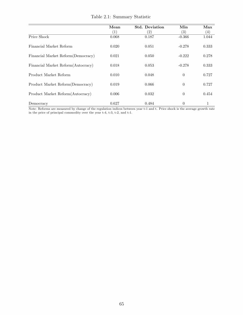
Table 2.1: Summary Statistic

Mean Std. Deviation Min Max(1) (2) (3) (4)

Price Shock 0.068 0.187 -0.366 1.044

Financial Market Reform 0.020 0.051 -0.278 0.333

Financial Market Reform(Democracy) 0.021 0.050 -0.222 0.278

Financial Market Reform(Autocracy) 0.018 0.053 -0.278 0.333

Product Market Reform 0.010 0.048 0 0.727

Product Market Reform(Democracy) 0.019 0.066 0 0.727

Product Market Reform(Autocracy) 0.006 0.032 0 0.454

Democracy 0.627 0.484 0 1

Note: Reforms are measured by change of the regulation indices between year t-1 and t. Price shock is the average growth ratein the price of principal commodity over the year t-4, t-3, t-2, and t-1.

65

Table 2.2: Estimation for Financial Market Reform

Model 1 Model 2 Model 3 Model 4 Model 5OLS OLS OLS OLS GMM

Price shock -0.011 -0.014**(0.007) (0.006)

Price shock in Autocracy -0.023*** -0.023*** -0.017**(0.008) (0.007) (0.007)

Price shock in Democracy -0.003 -0.004 -0.003(0.009) (0.009) (0.009)

Democracy 0.006 0.005 0.004 0.0004(0.004) (0.004) (0.004) (0.002)

Reformt−1 0.063** 0.120***(0.025) (0.026)

Country FE X X X X XYear FE X X X X XNumber of countries 81 81 81 81 81Observations 2,302 2,246 2,246 2,158 2,158

Note: The table presents estimates of the impact of commodity price shocks on Financial Market Reform. Dependent variableis reform index measured by change of the regulation indices. Price shock is the average growth rate in the price of principalcommodity over three years. All models control for state and year fixed effects. Standard errors in parentheses *** p<0.01, **p<0.05, * p<0.1

66

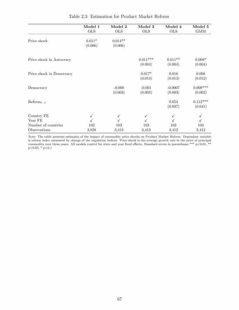
Table 2.3: Estimation for Product Market Reform

Model 1 Model 2 Model 3 Model 4 Model 5OLS OLS OLS OLS GMM

Price shock 0.011* 0.014**(0.006) (0.006)

Price shock in Autocracy 0.011*** 0.011** 0.008*(0.004) (0.004) (0.004)

Price shock in Democracy 0.017* 0.016 0.008(0.013) (0.013) (0.012)

Democracy -0.000 -0.001 -0.0007 0.009***(0.003) (0.003) (0.003) (0.002)

Reformt−1 0.054 0.112***(0.037) (0.041)

Country FE X X X X XYear FE X X X X XNumber of countries 103 103 103 103 103Observations 3,828 3,413 3,413 3,412 3,412

Note: The table presents estimates of the impact of commodity price shocks on Product Market Reform. Dependent variableis reform index measured by change of the regulation indices. Price shock is the average growth rate in the price of principalcommodity over three years. All models control for state and year fixed effects. Standard errors in parentheses *** p<0.01, **p<0.05, * p<0.1

67

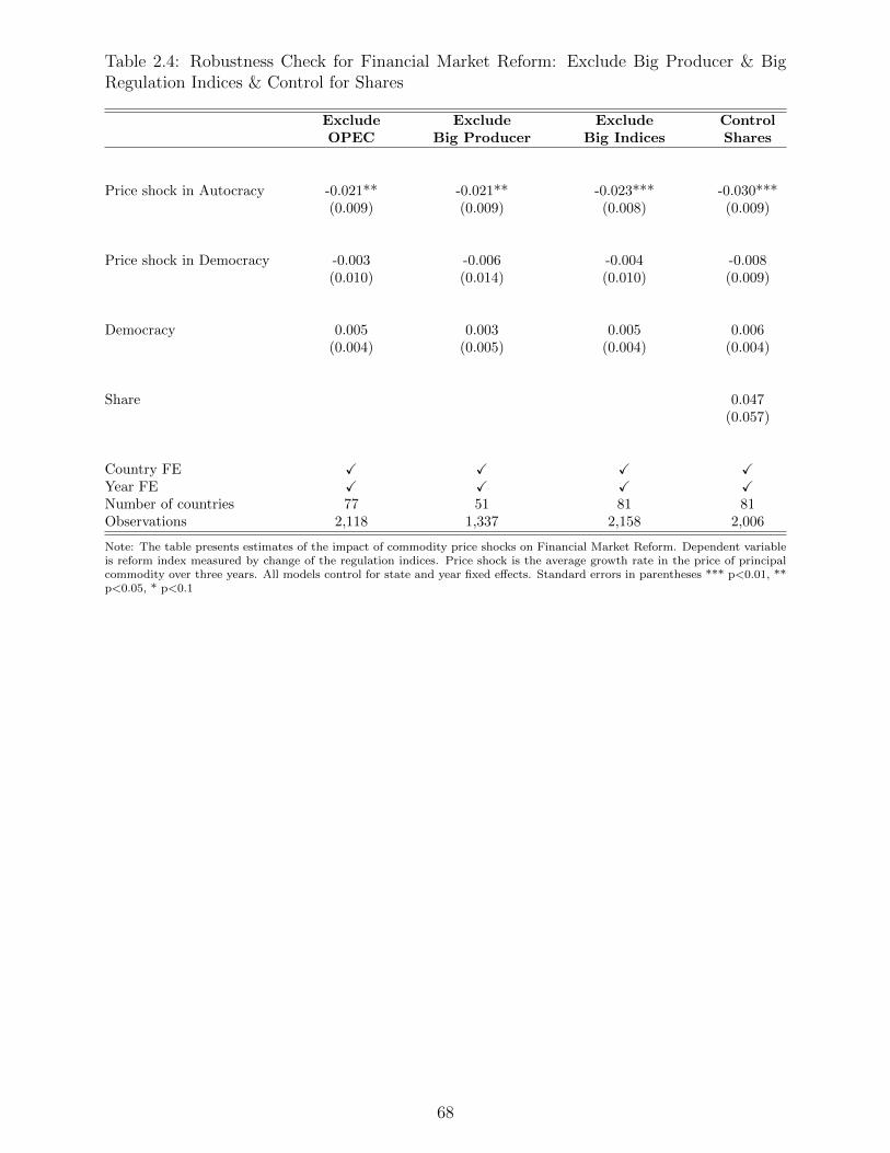
Table 2.4: Robustness Check for Financial Market Reform: Exclude Big Producer & BigRegulation Indices & Control for Shares

Exclude Exclude Exclude ControlOPEC Big Producer Big Indices Shares

Price shock in Autocracy -0.021** -0.021** -0.023*** -0.030***(0.009) (0.009) (0.008) (0.009)

Price shock in Democracy -0.003 -0.006 -0.004 -0.008(0.010) (0.014) (0.010) (0.009)

Democracy 0.005 0.003 0.005 0.006(0.004) (0.005) (0.004) (0.004)

Share 0.047(0.057)

Country FE X X X XYear FE X X X XNumber of countries 77 51 81 81Observations 2,118 1,337 2,158 2,006


68

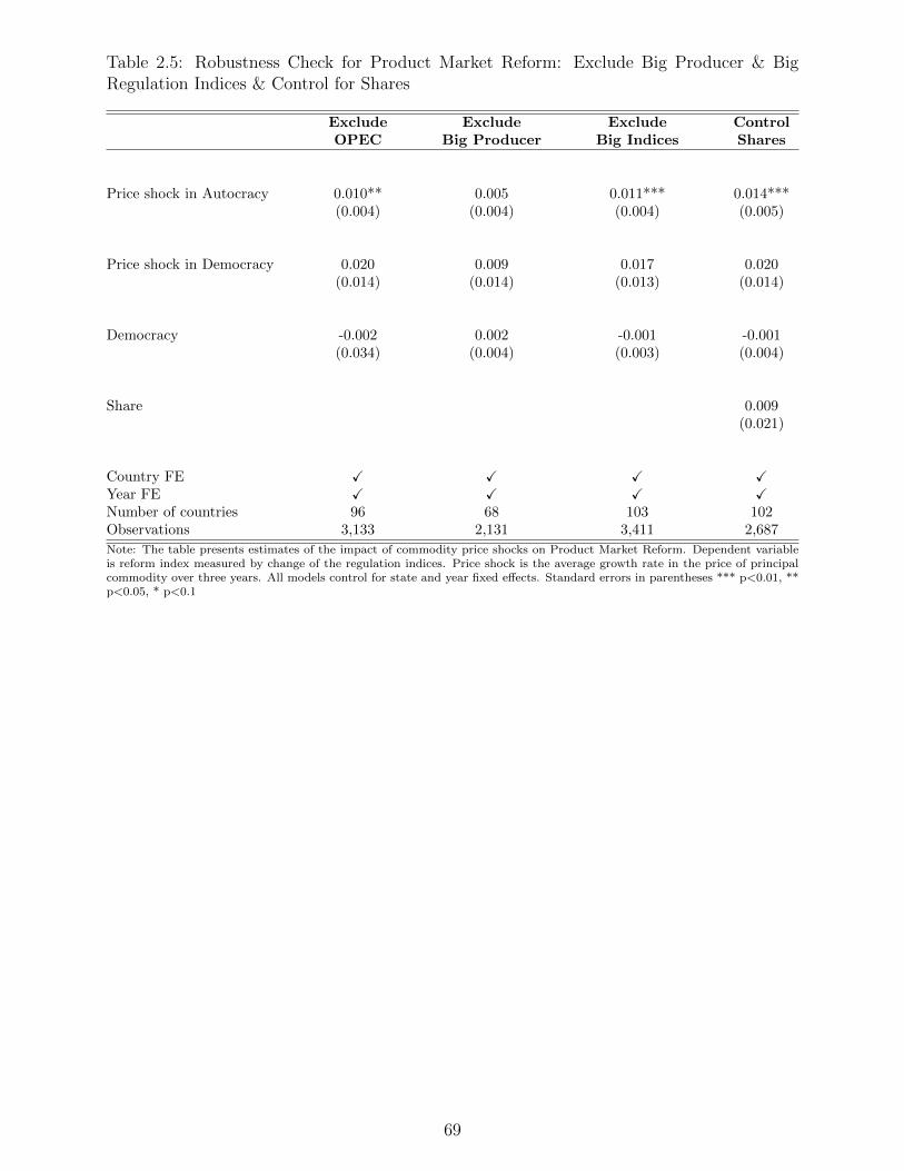
Table 2.5: Robustness Check for Product Market Reform: Exclude Big Producer & BigRegulation Indices & Control for Shares

Exclude Exclude Exclude ControlOPEC Big Producer Big Indices Shares

Price shock in Autocracy 0.010** 0.005 0.011*** 0.014***(0.004) (0.004) (0.004) (0.005)

Price shock in Democracy 0.020 0.009 0.017 0.020(0.014) (0.014) (0.013) (0.014)

Democracy -0.002 0.002 -0.001 -0.001(0.034) (0.004) (0.003) (0.004)

Share 0.009(0.021)

Country FE X X X XYear FE X X X XNumber of countries 96 68 103 102Observations 3,133 2,131 3,411 2,687


69

Table 2.6: Robustness Check for Financial Market Reform: Export Share

Exclude Exclude Placebo PlaceboFirst Quartile Below Median First Quartile Below Median

Price shock in Autocracy -0.020** -0.031*** -0.020 -0.013(0.009) (0.010) (0.023) (0.013)

Price shock in Democracy -0.006 -0.024* 0.012 0.011(0.011) (0.012) (0.013) (0.012)

Democracy 0.004 0.004 0.007 0.006(0.004) (0.005) (0.012) (0.006)

Country FE X X X XYear FE X X X XNumber of countries 56 30 25 51Observations 1,573 845 673 1401


70

Table 2.7: Robustness Check for Product Market Reform: Export Share

Exclude Exclude Placebo PlaceboFirst Quartile Below Median First Quartile Below Median

Price shock in Autocracy 0.015*** 0.015** -0.006 0.009(0.004) (0.006) (0.013) (0.007)

Price shock in Democracy 0.036** 0.034 -0.028 0.006(0.016) (0.024) (0.018) (0.016)

Democracy -0.003 0.002 0.010 -0.005(0.003) (0.004) (0.009) (0.005)

Country FE X X X XYear FE X X X XNumber of countries 75 47 28 56Observations 2,519 1,574 894 1839


71

Chapter 3

The Social Footprint of Bank

Regulation: Natural Experimental

Evidence from the US

3.1 Introduction

The large-scale deregulation of retail banking in the US in the second half of the

twentieth century has been causally linked to economic development (Jayaratne and

Strahan (1996)), more business start-ups (Black and Strahan (2002)), raised effi-

ciency in the banking sector (Jayaratne and Strahan (1998)), reduced income in-

equality (Beck et al. (2010)), improved access to college education of children from

credit-constrained (lower income) households (Sun and Yannelis (2016)) and other

outcomes.

72

While the economic benefits of deregulation of retail banking have often been

discussed in both academic and popular media, the social impacts are much less

well understood.1 In the US it lead, through increased competition in the local

retail banking markets, to a substantial increase in credit extended both to existing

borrowers and also to previously excluded households (Dick and Lehnert (2010)).

Given the central role that debt and financial stress have been shown to play in

depression (Bridges and Disney (2010)), mental health problems (Fitch et al. (2007)),

self-harm and suicide (Hatcher (1994)), suicidal thoughts (Hintikka et al. (1998)),

marital dissatisfaction (Grable et al. (2007)), intra-household conflict (Papp et al.

(2009)), domestic violence (Fox et al. (2002)) and other measures of personal or

family distress, it is natural to ask: Are there previously unaccounted for impacts of

the relaxation of regulation on important human distress metrics?

It is to this debate - what are the aggregate social consequence of freer access

to credit - that we aim to contribute here. Motivated by the research just cited

we focus on two suggestive metrics, namely; (1) rates of suicide and, (2) rates of

divorce. Noting the centrality of debt and financial circumstances in popular and

practitioner discussion of both outcome and divorce, and the important impact that

bank deregulation had on credit availability across the US, it is perhaps surprising

that the possible causal link between the two has not been explored rigorously before.

Cross-sectional analysis could be used to uncover any correlation between strin-

gency of banking regulation in a jurisdiction and rates of suicide and divorce. How-

1The two papers that speak to negative social impact are: (1) Dick and Lehnert (2010) estimatethat lifting of intrastate branching restrictions - which we will focus on here - caused a 10 to 16%increase in personal bankruptcies. (2) Garmaise and Moskowitz (2006) estimate that the samereform caused a decrease in property crime.

73

ever, deducing a causal relationship from any such correlation would be fraught with

danger. Jurisdictions with unobserved characteristics that lead to them to have less

regulated banking might plausibly have characteristics (the same, or other) that make

inhabitants of those jurisdictions more prone to suicide and/or divorce.

Here we overcome this methodological challenge by exploiting the staggered dereg-

ulation of intrastate banking rules across states during the 1970s, 1980s and 1990s.2

Importantly the timing of adoption of deregulation has been shown to be unrelated

to actual or anticipated state-level economic circumstances (Jayaratne and Strahan

(1996)).3 We will also confirm that timing of deregulation was uncorrelated with

state-level suicide and divorce rates, and carry out an unusually thorough set of

placebo exercises in which we repeatedly falsely assign treatment dates to states. A

significant number of papers, some already cited, have used the exogenous variation

in timing of treatment to underpin causal inference using a differences-in-differences

design. We do the same here, following the empirical approach of Sun and Yannelis

(2016), Dick and Lehnert (2010) and others more or less exactly.

So what do we expect to find? As should be clear, there are mechanisms that

plausibly push in opposing directions on our outcomes of interest. Making access to

credit easier can aid consumption smoothing - help individuals and families to remain

liquid during a temporary fall in income - can plausibly mitigate distress. On the

other hand looser credit can feed indebtedness problems and over-borrowing under

predatory lending practices (Bond et al. (2009)) or among those with self-control

2We will outline the institutional detail of this and other components of the deregulation of retailbanking later in the paper.

3Kroszner and Strahan (1999) provide a careful analysis of the economic and political reasonsfor the exact timing of state branching deregulations in various states.

74

problems (Gathergood (2012)), while Brown et al. (2005) and others evidence the

psychological burden of debt more generally. In this way, bank branching deregula-

tion could have negative social impacts. This makes the overall impact on distress

through diverse channels is an empirical question.4

As a preview of our main findings, we identify deregulation of intrastate branching

rules as overall causing a 3.3% increase in state-level suicide rate and a 4.7% increase

in the state-level divorce rate. To give an approximate feel for what that means,

the suicide number converts to around 1515 additional suicide deaths (and 37 100

additional suicide attempts) across the country per annum at an estimated cost of

USD 2.27 billion.5 Results are in most cases statistically significant at levels much

higher than 1%, and prove resilient in a variety of robustness checks and falsification

exercises.

The rest of the paper is organized as follows. Section 2 summarizes some perti-

nent literature on finance and psychological health, suicide and divorce. Section 3

describes our research setting - retail banking in the US and its deregulation between

1970 and the 1990s. Section 4 outlines data. Section 5 outlines empirical strategy.

Section 6 reports main results and those from a number of robustness checks and

falsification exercises. Section 7 concludes.

4Deregulation also spawned innovation and novel practices that could also have had positive ornegative impacts on personal distress. For example Melzer (2011) estimate that the advent andgrowth of the ‘payday loan’ industry, providing very short-term consumer loans at very high annu-alized interest rates, exacerbated indebtedness problems causing increased delinquency on mortgageand rent payments and deferral of needed health care.

5For these indicative numbers we simply interact the estimated percentage change with summarynational statistics and cost estimates for 2016 at afsp.org.

75

3.2 Literature Review

There are several strands of research that make plausible a causal link from avail-

ability of credit and the levels of suicide and divorce. While we will remain largely

agnostic on causal channels it is sensible to review mechanisms consistent with the

statistical results that we will present later in the paper. In this section we provide

brief sketches of research that links credit availability (and debt) to psychological

health, suicide and divorce.

Fitch et al. (2007) find that the greater availability of credit in the UK during the

past two decades has resulted in more mental health problems relating to increasing

debt. Expanded credit in the UK is mainly attributed to the deregulation of financial

markets in the 1980s and the entry of the US lenders into the UK market in 1990s.

Deregulation led to intensified competition, aggressive marketing and targeting of

new customer groups, including low income individuals. They report that one in four

people with mental health problems in the UK report having debt or arrears, three

times the prevalence compared to individuals without similar conditions. In similar

vein Bridges and Disney (2010) study the effect of household financial indebtedness

on psychological well-being using a large household survey of families with children

in Britain. The results show a strong association between being in a depressed

psychological state and metrics for indebtedness and financial stress. Gathergood

(2011) use changes in local housing prices as exogenous variation in the severity

of household debt (difficulties servicing debt) examine the causal impact of problem

debt on psychological health, finding the similar results on the link from indebtedness

76

to psychological stress.

In the medical literature, some studies suggest that debt is linked to psychological

distress including depression and anxiety. Reading and Reynolds (2001) suggest

that financial adversity has a central place in the association between socioeconomic

hardship and maternal depression. They use longitudinal data, collected over six

months, on 271 families with young children and find that stress about debt was the

strongest independent socioeconomic predictor of the depression score in repeated

interviews.

A large literature points to an association between debt problems and suicide.

Hatcher (1994) provides a descriptive survey of financial difficulties in a consecutive

series of patients who deliberately poisoned themselves in the UK. Their study sug-

gests that the patients in debt were more likely to harm themselves with greater

suicidal intent and subsequently to report more symptoms of depression and hope-

lessness. Hintikka et al. (1998) use data from Finnish general population and also

find that difficulties in repaying debts were associated with suicidal ideation and sui-

cide attempts. Yip et al. (2007) find that the presence of indebtedness is a risk factor

that can trigger stressed individuals to contemplate suicide, using data from Hong

Kong. They further attribute unmanageable debt to increasing credit availability in

that jurisdiction, particularly to previously excluded groups.6

Evidence also show that suicide rates increase during periods of economic reces-

6The relationship between debt and suicide is also found in the developing world. Merriott(2016) reviews a broad set of literature concerning factors associated with the farmer suicide crisisin India, where an estimated 16 000 farmers commit suicide annually (far above the rate in the widerpopulation). After reviewing the literature which identified numerous factors, the author concludesthat increased indebtedness (and inability to service debt in the face of income fluctuations) playedthe predominant role in farmer suicides.

77

sion. Frasquilho et al. (2015) demonstrate that periods of economic recession are

associated with a higher prevalence of mental health problems, including common

mental disorders, substance disorders, and ultimately suicidal behaviour thorough

analysis of the selected investigations. One financial stress that were identified as

contributing to mental health problem and suicidal behaviour is debt from loans,

mortgage/rent arrears, and debt to friends and family in 2008 Global Financial Cri-

sis (Gunnell et al. (1998)). Coope et al. (2014) investigated trends in indicators of the

2008 economic recession and trends in suicide rates in England and Wales and find

that the indicators of economic strain other than unemployment and redundancies,

such as personal debt and house repossessions contribute to increased suicide rates

in younger-age men.

There is a well-documented statistical association between financial stress in

within families and divorce. Divorce is determined by many factors, while financial

issues play a more significant role relative to other common marital disagreements.

Papp et al. (2009) analyze diary reports of 748 marital conflict instances from 200

married people. They find that compared to non-monetary issues, marital conflicts

about money were more pervasive, problematic, and recurrent, and more likely to

remain unresolved. In addition, Dew et al. (2012) claim that financial disagreements

are more salient to couples, are less easily resolved, and lead to more problematic

conflicts compared to other common disagreements. Financial satisfaction is strongly

linked to marital satisfaction. Grable et al. (2007) investigate the role financial satis-

faction has on the thought of subsequent divorce and find that individuals with high

levels of financial satisfaction were significantly less likely to have thought about di-

78

vorce during the past three years. Financial distress such as debt is likely to induce

divorce. For example, consumer debt could lead to marital conflict. Dew (2007) finds

that consumer debt directly predicts higher frequency in marital conflict. Spouses

may disagree on the desirability, necessity, and practicality of assuming debt and

these disagreements may strain marriages.7

3.3 Setting

Historically almost all US states restricted banks from expanding geographically both

within and across state borders. With regards to intrastate restrictions, some states

allowed bank holding companies to own separately capitalized and licensed banks

throughout the state, while others were “unit banking states” in which each bank

was permitted to operate only one office. Between the 1970s and mid-1990s these

restrictions were removed state by state. This is widely regarded a wholesale relax-

ation of regulation in the sector, and drove substantial changes in the organization

and operation of the sector and the supply of credit to households.

Consistent with most existing studies (Beck et al. (2010), Sun and Yannelis

(2016)) we will define our date of deregulation as the year in which a state legal-

ized intrastate branching via mergers and acquisitions through the holding company

structure.8

7An alternative view, and one implying as more upbeat view of divorce, is that the availability ofcredit could facilitate an amicable break-up in a setting in which finances would otherwise oblige acouple to remain married. While we will treat marital breakdown as a metric for social distress werecognize the need to be more cautious in interpreting the welfare impacts of an increase in divorcerates. The necessarily negative implication of suicide is less contentious.

8This was the first major deregulatory step and in most cases was followed by lifting of restrictionson de novo branching (allowing a bank holding company to establish a new branch in a different

79

Our identification will exploit the fact that the timing of deregulation was stag-

gered across states. The progress of deregulation is summarized in figure 3.1 and

table 3.1. At the start of the 1970s only 12 states allowed intrastate branching, by

1996 only Arkansas, Iowa and Minnesota had not lifted restrictions. The important

paper by Jayaratne and Strahan (1996) was the first to provide compelling evidence

that dates of deregulation were not explained by state-level variations in economic

conditions (actual or anticipated) and so for our analysis can plausibly be treated as

exogenous.

3.4 Data

To investigate the effect of branch deregulation on suicide and divorce, we gather

data on the timing of bank deregulations, suicide rates, divorce rates and other state

level characteristics. We derive data form several sources. We study the twenty year

period from 1976 to 1996.

Dates of deregulation were taken from Kroszner and Strahan (1999). Certain

peculiarities of the banking sector in Delaware and South Dakota lead us to drop

those two states form our main sample, consistent with most other studies in the

literature (Beck et al. (2010), Dick and Lehnert (2010)). As a robustness check we

will confirm that reinserting them has little impact on results.

Data on suicide are from National Center for Health Statistics (NCHS). The

NCHS is the primary health statistics agency in the US and compiles and dissemi-

nates statistical information on a plethora of health issues. The suicide data we use

geographical area). See Sun and Yannelis (2016) for a more thorough review.

80

are derived from their ongoing census of death certificates (which record causes of

death). We obtain measures of suicide per capita for each state for each year in our

study period. Data on completed divorces on the same basis also come from the

NCHS.

To account for time-varying changes in a state-level economic conditions we will

use a number of control variables, including state unemployment rate, state personal

income, age composition and racial composition. Personal income is the natural log

of state personal income per capita. Age composition variables measure the share of

the population of a state in a series of ten-year cohort ‘bins’. Racial composition to

is the share of the population in the state that is black, white, or other. Age and

race data are constructed from Unicon’s March CPS files, and refer to the population

aged fourteen years or greater.

Table 3.2 provide summary statistics. With respect to our outcome variables of

interest, the average number of suicides in our sample across the whole period is 130

per million of population per annum. The average number of divorces is 5225 per

million of population per annum.

3.5 Empirical Strategy

Our source of identifying variation is the plausibly exogenous variation in timing of

bank branching deregulation across states.

We use this natural variation to explore causal effects from deregulation to our

chosen metrics of social distress (suicide and divorce) using state-based panel esti-

81

mation, including both state and time fixed effects in all regressions. To capture

exposure to our treatment, deregulated banking, we use a dummy. We estimate

Yit = βDeregulationit + γXit + αi + τt + εit (3.1)

The dependent variable Yit is the suicide or divorce rate in state i in year t. The

binary variable Deregulationit takes the value 1 if intrastate branching was allowed

in state i in year t. Xct is a vector of other regressors and includes controls for state

unemployment rate, state personal income, and indicator variables capturing age

composition and racial composition of population at state level. The specification also

includes year fixed effects (τt) that control for national trends in suicide and divorce,

and any time-varying factors that influence suicide and divorce at the national level,

and state fixed effects (αi) that control for any time-invariant factors that influence

suicide and divorce at state level.

Standard errors are calculated using the block bootstrap method to allow for po-

tential serial correlation. Block bootstrap maintains the autocorrelation structure by

keeping all the observations that belong to the same state together. Block bootstrap

methods are widely applied in the difference-in-differences literature (Sun and Yan-

nelis (2016), Bertrand et al. (2004)). Using Monte Carlo simulation, Bertrand et al.

(2004) demonstrate that block bootstrap (taking into account the autocorrelation of

the data) works well when the number of states is large (50 in their case).

The specification is a generalization of the difference-in-differences approach Bertrand

et al. (2004), Imbens and Wooldridge (2009). The coefficient of interest in each case

is β. The difference-in-differences method is appropriate when the timing of inter-

82

vention is as good as random, conditional on time, and group fixed effects. Validity

of our approach requires that timing of deregulation by state not be systematically

related to pre-existing levels suicide or divorce. While such a relationship seems un-

likely, to dispel any residual concern we follow the previous literature (Beck et al.

(2010)) by generating scatter-plots from year of deregulation to each of our outcome

variables. These are presented in figure 3.2 and figure 3.3. Visually there is no

discernible pattern to either scatter, and the lack of correlation is confirmed by the

calculations reported in the figure notes.

3.6 Results

3.6.1 Main Results: Suicide

Table 3.3 reports results with state-level suicide rate as the dependent variable.

Column (1) includes no controls except state and year fixed effects. The coefficient

on the deregulation regressor is positive and statistically significant at 5% (p value =

0.023). In columns (2) through (4) we introduce, individually and together, standard

proxies for state-level economic conditions (unemployment rate and personal income).

Unemployment is positively associated with suicide, income negatively. However, of

interest to us is that the estimated coefficient on deregulation is largely undisturbed

by their inclusion.

We use annual data throughout. However the date within a year at which regu-

lation is relaxed varies between states. Further, it is likely that it would take at least

several months following the date of deregulation for practical consequences to be

83

felt. To account for this we re-estimate the specification in column (4) but excluding

data relating to the year in which reform occurred and the first year calendar year

after reform. The results of this exercise are reported in column (5). The coefficient

remains positive and significant at 1% (p value = 0.004).

Column (5) represents our preferred specification. The suicide rate average across

our sample is 130 per million implying that bank deregulation causes a 3.3% increase

in the state level suicide rate.

3.6.2 Main Results: Divorce

Table 3.4 reports results from conducting the same exercises but with state-level

suicide rate replaced by state-level divorce rate as the dependent variable.

In each column the estimated coefficient on the deregulation regressor is positive

and significant at better than 1%. The estimates can again be seen to be compar-

atively insensitive to inclusion or exclusion of proxies for time-varying state-level

economic conditions.

Our preferred specification is again column (5), which generates an estimated

coefficient of interest of 243.6, significant at better than 1% (p value = 0.000). The

average state level divorce rate in our sample is 5224 per million implying that

deregulation causes a 4.7% increase in the state-level divorce rate.

3.6.3 Robustness

Table 3.3 and table 3.4 presented our preferred specifications. In addition to the

preferred specifications other columns provided some evidence of the stability of our

84

estimated coefficients of interest to the inclusion or exclusion of a key state level

controls (proxies for time-varying, state-specific economic conditions).

In this section we subject our main results to a number of other robustness chal-

lenges.

Demographics Suicide and divorce propensities have been shown to vary with age

and race (Preti and Miotto (1998), Kubrin and Wadsworth (2009), Michael (1978),

Bulanda and Brown (2007)). These demographic profiles vary across state and evolve

through time, which could lead to changing patterns of suicide and divorce. We have

no reason to think those variations would correlate with timing of bank deregulation.

However to investigate any potential confounding factors we re-estimate our main

specifications but now including a set of indicator variables for age and race compo-

sition by state, by year (described in data section). The results of this are reported

in column (1) of each of table 3.5 and table 3.6. The estimated coefficient on the

bank deregulation variable remain positive and significant at better than 1% with

value little disturbed.

Outliers A legitimate question in any analysis of this sort is the role of outliers -

to what extent are the results of our main regressions driven by things happening in

a single or small number of states.

We address this in two ways. In Appendix table 3.7 and Appendix table 3.8 we

re-estimate our preferred specification but excluding in turn each of the five most

populous states (in order, California, New York, Texas, Pennsylvania and Florida).

It can be seen that in few case is sign or statistical significance lost. In 9 out of the

85

10 exercises the coefficient value is little changed, though when considering suicide

as the outcome excluding California reduces the coefficient estimate by around a

quarter.

Separately we execute a 99% winsorization of data. By winsorizing the impact of

outliers is reduced, without losing observations. Column (2) of table 3.5 and table 3.6

summarize the results of reestimating of our preferred specification with the adjusted

data. Results are not substantially impacted (though as expected implied effect sizes

are muted somewhat) allaying concerns that inference is based on outliers.

Delaware and South Dakota Following Beck et al. (2010), Dick and Lehnert

(2010) and others we excluded Delaware and South Dakota from our dataset. His-

torically they had quite different banking policy environments (for example, tax

incentivized credit card lending by banks) such that banking reform in these states

had a different structure, and can be expected to have had different impacts. While

these exclusions are warranted, for each outcome variable we reestimate our preferred

specification but reinserting these two states into the panel. The results of this ex-

ercise are reported in column (3) of each of table 3.5 and table 3.6. The results are

similar to our main results.

Divorce law Another threat to identification arises from the recognition that, in

addition to deregulating banking, many states during this same period reformed

divorce laws. In particular they enacted unilateral divorce legislation that allowed

for either party to initiate dissolution of a marriage without seeking the approval of

the other. Stevenson and Wolfers (2006) and Friedberg (1998) present evidence of

86

a causal effect of such reform on suicide and divorce. As such we want to address

concerns that the state-level changes in suicide and divorce rates that we attribute

to bank reform are not in fact a result of changes to divorce laws happening around

the same period.

We do this in two ways. The first is to confirm that there is little or no correlation

between the timing of bank deregulation and that of divorce law reform. This we do

in Appendix figure 3.6. Visually there is no discernible pattern in the scatter-plot,

and the correlation coefficient is -0.04. This makes divorce law reform unlikely to be

an important confounder in our exercise. Nonetheless in column (4) of table 3.5 and

table 3.6 we re-estimate our preferred specifications but now inserting a dummy vari-

able that takes the value 1 if in state i in period t prevailing divorce law allowed for

unilateral divorce. In each case our estimated coefficients on bank regulation changes

only slightly but the precision of the estimate (and level of statistical significance) is

improved.

Lagged unemployment Unemployment has been shown to be an important con-

tributor to both of our outcomes of interest, with effects sometimes spilling over

between years (Beck et al. (2010)). In Appendix table 3.9 and Appendix table 3.10

we add three lags of the unemployment rate, both individually and as a suite, to

our main specification. Again, our main results are not significantly disturbed - the

implied effect sizes are if anything somewhat larger.

87

3.6.4 Falsification: Evidence from 6000 Placebos

While our interest is the uncovering of a causal effect (should one exist) of bank

deregulation on suicide or divorce, the variation that we exploit is with respect to

date of treatment.

Inclusion of year fixed effects controls for any time-varying, across-state factors

that might have been influencing suicide or divorce rates during our study period.

This includes factors particular to a single year as well as longer-term trends or cycles.

We have also verified that timing of deregulation was not systematically related to

pre-deregulatory levels of our outcome variables.

To further challenge our identification, in this section we report the results of

running a large number of placebo tests. In each of these we falsely assign other,

counterfactual treatment dates.

Placebo exercises are a test of design (Chetty et al. (2016), Card et al. (2012)).

If when we work with a vector of state-level deregulation dates that we know to be

false the regression exercise generates a significant coefficient, then we know that

‘result’ to be spurious. Of course in any given such exercise such significance could

be generated by chance. To endorse our design we want to be convinced that such

spurious outcomes do not occur too often.9

With this in mind, for each of three different ways of randomly-assigning false

treatment dates to states, for each outcome variable, we run 1000 placebo regres-

sions and from each regression harvest the estimated coefficient on the deregulation

9Of the papers that we have cited so far on the effects of deregulation none presents the resultsof any placebo exercises.

88

regressor and associated t values. In other words we end up with 6000 β’s and 6000

t values. From this we can assess how likely it is that the values from our preferred

specifications (with correctly assigned treatment dates) would have been generated

spuriously.

Placebo 1 (Preferred) In the first exercise we construct a list of dates at

which a state deregulated, allowing repetition. So for example the year 1988 ap-

pears on the list four times, because four states (Illinois, Louisiana, Oklahoma and

Texas) deregulated in that year, while 1979 (Ohio) appears only once. To construct

a placebo vector of deregulation dates, for each state we draw at random a date

from that list. If the date happens to coincide with the true date for a particular

state it is discarded and another date is drawn. We do this repeatedly to construct

1000 different placebo vectors. For each placebo vector we reestimate our preferred

specifications (corresponding to column (5) in table 3.3 and table 3.4).

Placebo 2 In the second exercise, to construct a placebo vector of deregulation

dates for each state we draw a year at random from the dates 1960 to 1999 (the

whole period of the bank deregulation wave). If the date happens to coincide with

the true date for a particular state it is discarded and another date is drawn. We do

this repeatedly to construct 1000 different placebo vectors then proceed as above.

Placebo 3 In placebo 3 we proceed as in placebo 1, but not allowing repetition.

In other words any particular date can appear at most once on the list. To construct

a placebo vector of deregulation dates, for each state we draw at random a date from

89

that list. If the date happens to coincide with the true date for a particular state

it is discarded and another date is drawn. We do this repeatedly to construct 1000

different placebo vectors then proceed as above.

Falsification Results

The results of these exercises for suicide as outcome variable are presented in figure

3.4.

The barchart in the left-hand of the top panel plots the 1000 coefficients derived

form placebo exercise 1. The right-hand panel plot the T values. The vertical line

in each case denotes the coefficient from the true assignment. Only 12/1000 (or

1.2%) placebo runs deliver a coefficient estimate bigger than the 4.28 under true

assignment, and 14/1000 (1.4%) deliver a bigger T value.

The middle and bottom panels present equivalent barcharts corresponding to

placebos 2 and 3 respectively. In each case it can be seen that the coefficients and

T values from the regressions under true assignment are far in the right-hand tail of

the distributions. The numbers of cases are summarized in the table underneath. In

the least favorable case (here placebo 2) the coefficient value and t value under true

assignment lie above 97.0% and 97.1% of those from the placebo regressions.

Figure 3.5 presents the results of the same falsification exercises but with divorce

as the outcome variable. Again the results are similar. In the least favorable case

(placebo 2) the coefficient value and t value under true assignment lie above 97.6%

and 97.8% of those from the placebo regressions.

Taken together we believe that these results make it unlikely that the pattern

90

characterized in our main tables are spurious or underpinned by shortcomings with

design.

3.7 Conclusion

Banks play a vital role in supporting economic and social activity by extending credit

and other services to individuals and businesses. The relaxation of branch banking

restrictions in most American states between the 1970s and 1990s led to increased

competition between banks (Jayaratne and Strahan (1998)) and lower prices and

higher quantities of credit. As a result individuals borrow more to buy homes (Tewari

(2014)), start businesses (Black and Strahan (2002)) and pay for education (Sun

and Yannelis (2016)). Total private loan volume increases, bank fees decrease, and

mortgage loan interest rates decrease after branching deregulation takes effect (Sun

and Yannelis (2016)).

However as gatekeepers to credit, banks are also central participants in the cre-

ation of debt. What are the implications of loosening regulation of banks on social

outcomes? Garmaise and Moskowitz (2006) found a significant negative effect on

property crime. Dick and Lehnert (2010) found a significant positive effect on per-

sonal bankruptcy. The important impacts that access to credit can have on individual

and familial distress motivated us to investigate a possible causal influence of dereg-

ulation on patterns of suicide and divorce. Since these impacts can be positive or

negative, the overall impact is an empirical question.

The analysis reported here points to a significant and robust causal impact of

91

deregulation of branching rules on state-level measures of suicide and divorce rates.

The effect size is substantial. In our preferred specification it causes a 3.3% increase

in state-level suicide rate and a 4.7% increase in the state-level divorce rate. Results

are in most cases statistically significant at levels much higher than 1%, and prove

resilient in a variety of robustness checks and falsification exercises.

These empirical findings are consistent with the relaxation credit supply being

the primary mechanism through which this financial deregulation affected suicide

and divorce. We did not provide direct test on the credit availability as the mecha-

nism, but the banking deregulation literature suggest that banks in general allowed

previously excluded households to enter the market and increased overall personal

borrowing, including credit card loans (Dick and Lehnert (2010), Sun and Yannelis

(2016)).

The analysis adds further nuance to the intricate inter-relationship between retail

banking sector and social lives, and that care is needed in thinking about how the

provision of credit should be managed and regulated.

92

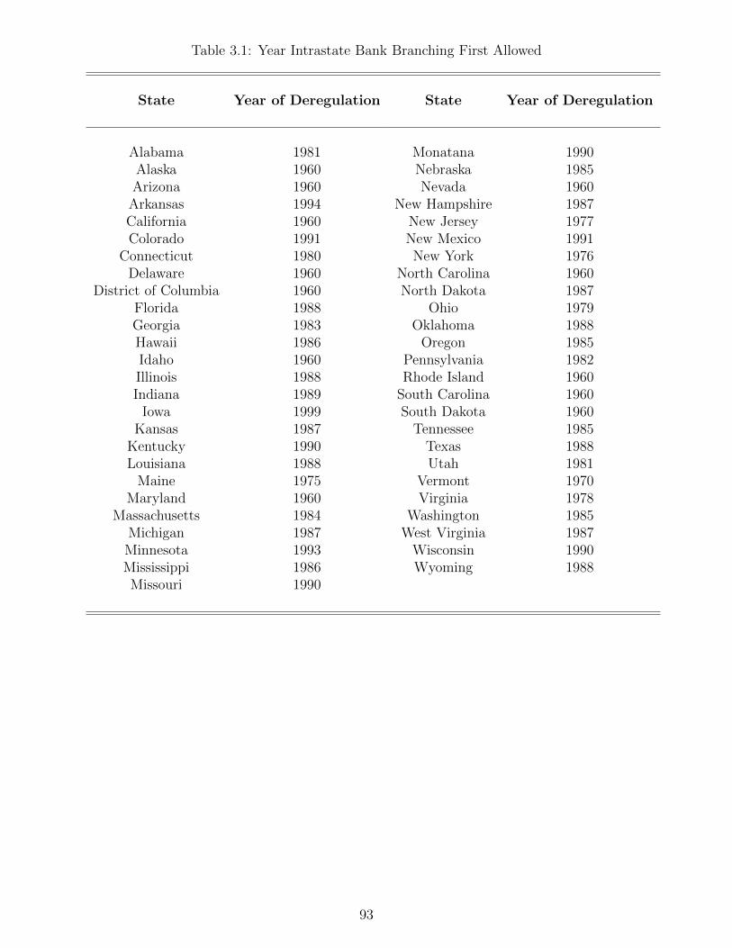
Table 3.1: Year Intrastate Bank Branching First Allowed

State Year of Deregulation State Year of Deregulation

Alabama 1981 Monatana 1990Alaska 1960 Nebraska 1985Arizona 1960 Nevada 1960Arkansas 1994 New Hampshire 1987California 1960 New Jersey 1977Colorado 1991 New Mexico 1991

Connecticut 1980 New York 1976Delaware 1960 North Carolina 1960

District of Columbia 1960 North Dakota 1987Florida 1988 Ohio 1979Georgia 1983 Oklahoma 1988Hawaii 1986 Oregon 1985Idaho 1960 Pennsylvania 1982Illinois 1988 Rhode Island 1960Indiana 1989 South Carolina 1960

Iowa 1999 South Dakota 1960Kansas 1987 Tennessee 1985

Kentucky 1990 Texas 1988Louisiana 1988 Utah 1981

Maine 1975 Vermont 1970Maryland 1960 Virginia 1978

Massachusetts 1984 Washington 1985Michigan 1987 West Virginia 1987Minnesota 1993 Wisconsin 1990Mississippi 1986 Wyoming 1988Missouri 1990

93

Table 3.2: Summary Statistics

Mean Std. Deviation Min Max(1) (2) (3) (4)

Suicide Rate (per 1,000,000) 130.229 33.617 51.245 288.133Divorce Rate (per 1,000,000) 5224.848 1813.538 2037.666 17600Unemployment Rate 0.07206 0.02337 0.02141 0.18771Personal Income 9.5339 0.4081 8.4674 10.3974Share 14-19 0.1226 0.0220 0.0645 0.1926Share 20-29 0.2111 0.02944 0.1303 0.3370Share 30-39 0.1995 0.02717 0.1298 0.2910Share 40-49 0.1493 0.0237 0.0935 0.2298Share 50-59 0.1204 0.0138 0.0758 0.1647Share 60-69 0.1035 0.0150 0.0318 0.1722Share 70-79 0.0662 0.0142 0.0126 0.1140Share 80-89 0.0244 0.0071 0.0005 0.0497Share 90plus 0.0031 0.0017 0.0000 0.0096White Share 0.8620 0.1414 0.2323 0.9994Black Share 0.1005 0.1199 0.0000 0.7399Other Share 0.0374 0.0953 0.0000 0.7567

Note: Suicide and divorce rate is per 1,000,000. Personal income is the natural log of state personal income per capita. Agecomposition variables indicate the share of states’ populations aged 14 to 19, and then ten-year cohorts beginning with age 20up to a variable for 90+. Racial composition refers to the share of the state’s population that is Black, White, and other. Ageand race data are constructed from Unicon’s March CPS files, and refer to the population aged fourteen years or greater.

94

Table 3.3: Main Result: Suicide

Model Model Model Model Model(1) (2) (3) (4) (5)

Bank Deregulation 2.972** 3.308** 3.015** 3.227** 4.281***(1.303) (1.314) (1.320) (1.451) (1.502)

Unemployment Rate 74.831*** 48.523 55.478**(25.582) (31.455) (27.053)

Personal Income -32.879** -28.171* -32.815*(15.290) (16.347) (18.250)

State FE X X X X XYear FE X X X X XObservations 1,029 1,029 1,029 1,029 956R-squared 0.8772 0.8782 0.8791 0.8795 0.8804Note: Dependent variable is state suicide rate per annum per million of population. Bank deregulation equals one during allyears in which a state permits intrastate branching and equals zero otherwise. All models control for state and year fixed effects.Standard errors calculated using block bootstrap method in parentheses *** p<0.01, ** p<0.05, * p<0.1

95

Table 3.4: Main Result: Divorce

Model Model Model Model Model(1) (2) (3) (4) (5)

Bank Deregulation 202.426*** 197.831*** 204.361*** 209.719*** 243.607***(68.979) (73.329) (61.691) (64.962) (67.251)

Unemployment Rate -1507.890 1728.659* 2224.124*(1049.693) (1035.523) (1159.11)

Personal Income 3415.894*** 3576.127*** 3727.999***(417.696) (434.733) (406.790)

State FE X X X X XYear FE X X X X XObservations 986 986 986 986 915R-squared 0.9197 0.9199 0.9269 0.9271 0.9281Note: Dependent variable is state divorce rate per annum per million of population. Bank deregulation equals one during allyears in which a state permits intrastate branching and equals zero otherwise. All models control for state and year fixed effects.Standard errors calculated using block bootstrap method in parentheses *** p<0.01, ** p<0.05, * p<0.1

96

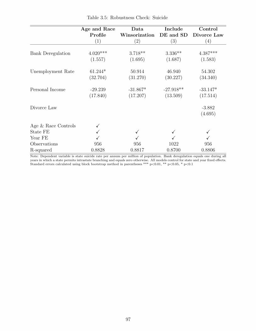
Table 3.5: Robustness Check: Suicide

Age and Race Data Include ControlProfile Winsorization DE and SD Divorce Law

(1) (2) (3) (4)

Bank Deregulation 4.020*** 3.718** 3.336** 4.387***(1.557) (1.695) (1.687) (1.583)

Unemployment Rate 61.244* 50.914 46.940 54.302(32.704) (31.270) (30.227) (34.340)

Personal Income -29.239 -31.867* -27.918** -33.147*(17.840) (17.207) (13.509) (17.514)

Divorce Law -3.882(4.695)

Age & Race Controls XState FE X X X XYear FE X X X XObservations 956 956 1022 956R-squared 0.8828 0.8817 0.8700 0.8806Note: Dependent variable is state suicide rate per annum per million of population. Bank deregulation equals one during allyears in which a state permits intrastate branching and equals zero otherwise. All models control for state and year fixed effects.Standard errors calculated using block bootstrap method in parentheses *** p<0.01, ** p<0.05, * p<0.1

97

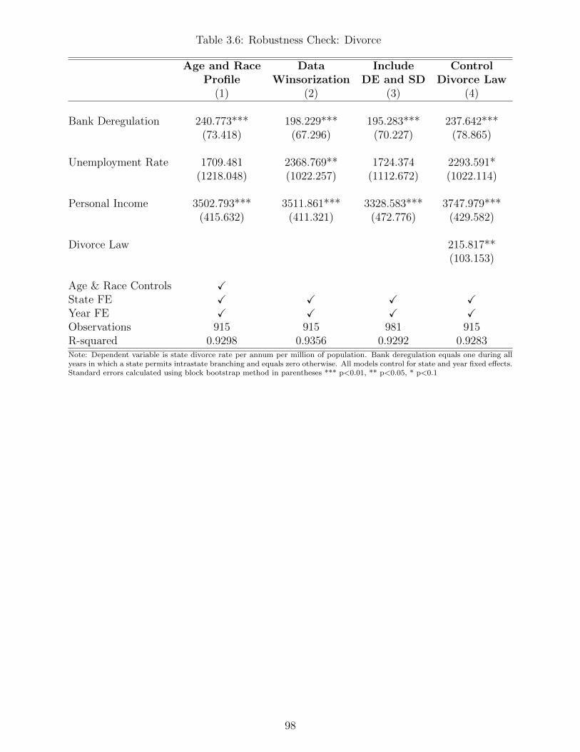
Table 3.6: Robustness Check: Divorce

Age and Race Data Include ControlProfile Winsorization DE and SD Divorce Law

(1) (2) (3) (4)

Bank Deregulation 240.773*** 198.229*** 195.283*** 237.642***(73.418) (67.296) (70.227) (78.865)

Unemployment Rate 1709.481 2368.769** 1724.374 2293.591*(1218.048) (1022.257) (1112.672) (1022.114)

Personal Income 3502.793*** 3511.861*** 3328.583*** 3747.979***(415.632) (411.321) (472.776) (429.582)

Divorce Law 215.817**(103.153)

Age & Race Controls XState FE X X X XYear FE X X X XObservations 915 915 981 915R-squared 0.9298 0.9356 0.9292 0.9283Note: Dependent variable is state divorce rate per annum per million of population. Bank deregulation equals one during allyears in which a state permits intrastate branching and equals zero otherwise. All models control for state and year fixed effects.Standard errors calculated using block bootstrap method in parentheses *** p<0.01, ** p<0.05, * p<0.1

98

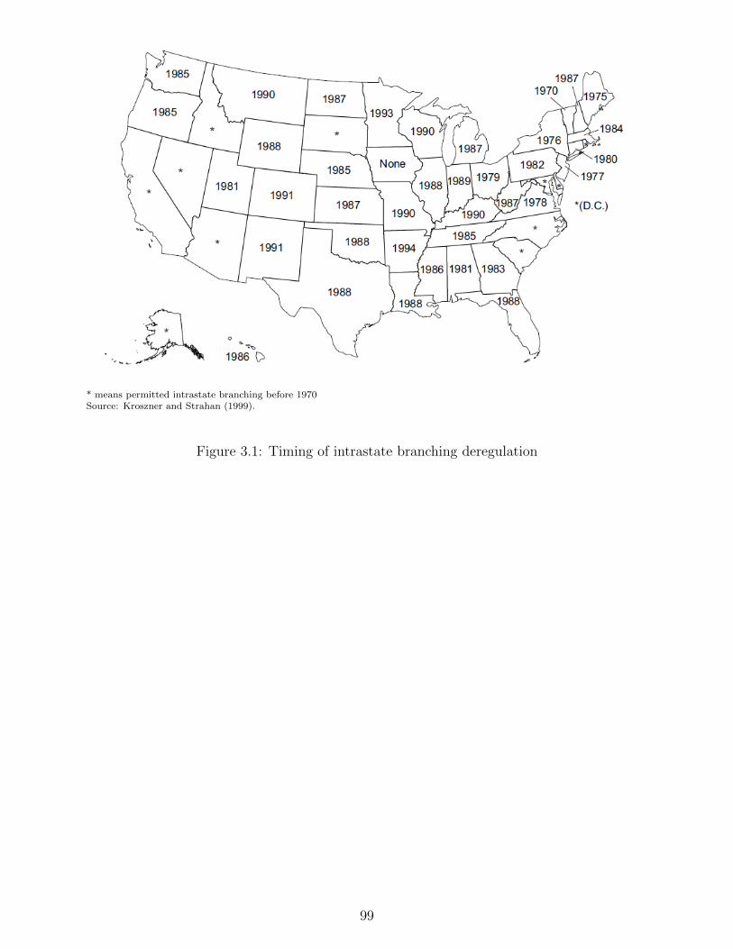
* means permitted intrastate branching before 1970Source: Kroszner and Strahan (1999).

Figure 3.1: Timing of intrastate branching deregulation

99

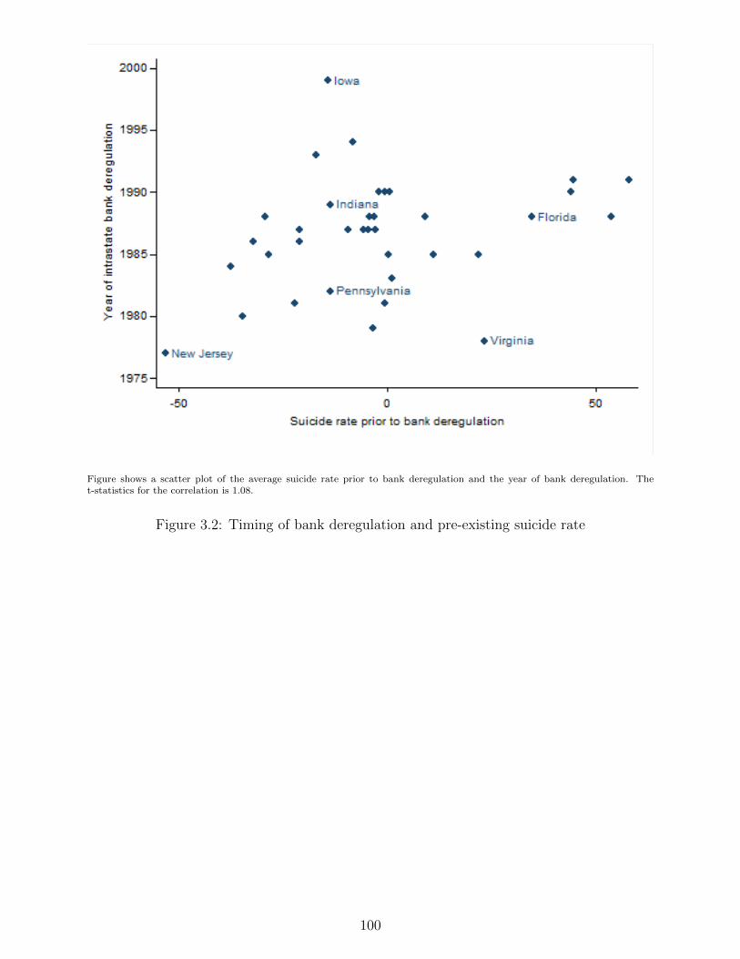
Figure shows a scatter plot of the average suicide rate prior to bank deregulation and the year of bank deregulation. Thet-statistics for the correlation is 1.08.

Figure 3.2: Timing of bank deregulation and pre-existing suicide rate

100

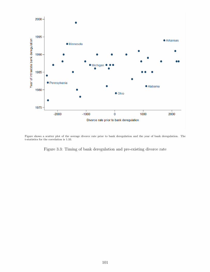
Figure shows a scatter plot of the average divorce rate prior to bank deregulation and the year of bank deregulation. Thet-statistics for the correlation is 1.33.

Figure 3.3: Timing of bank deregulation and pre-existing divorce rate

101

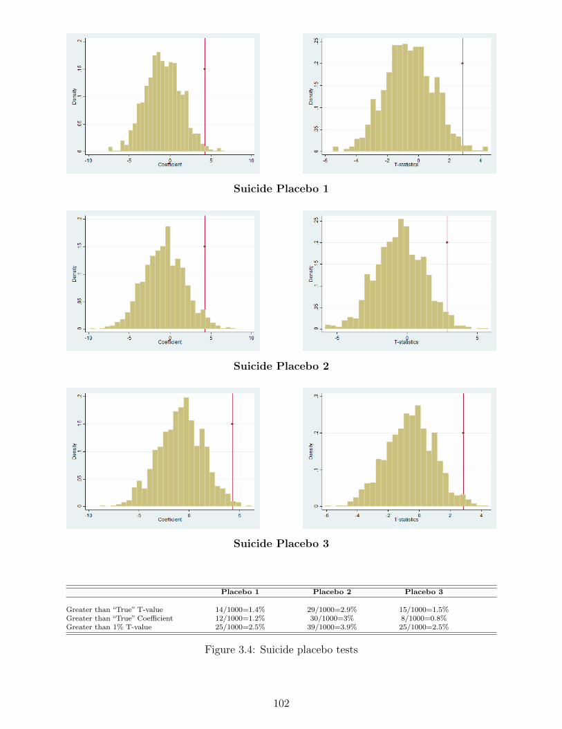
Suicide Placebo 1

Suicide Placebo 2

Suicide Placebo 3

Placebo 1 Placebo 2 Placebo 3

Greater than “True” T-value 14/1000=1.4% 29/1000=2.9% 15/1000=1.5%Greater than “True” Coefficient 12/1000=1.2% 30/1000=3% 8/1000=0.8%Greater than 1% T-value 25/1000=2.5% 39/1000=3.9% 25/1000=2.5%

Figure 3.4: Suicide placebo tests

102

Divorce Placebo 1

Divorce Placebo 2

Divorce Placebo 3

Placebo 1 Placebo 2 Placebo 3

Greater than “True” T-value 16/1000=1.6% 22/1000=2.2% 17/1000=1.7%Greater than “True” Coefficient 15/1000=1.5% 24/1000=2.4% 16/1000=1.6%Greater than 1% T-value 41/1000=4.1% 71/1000=7.1% 49/1000=4.9%

Figure 3.5: Divorce placebo tests

103

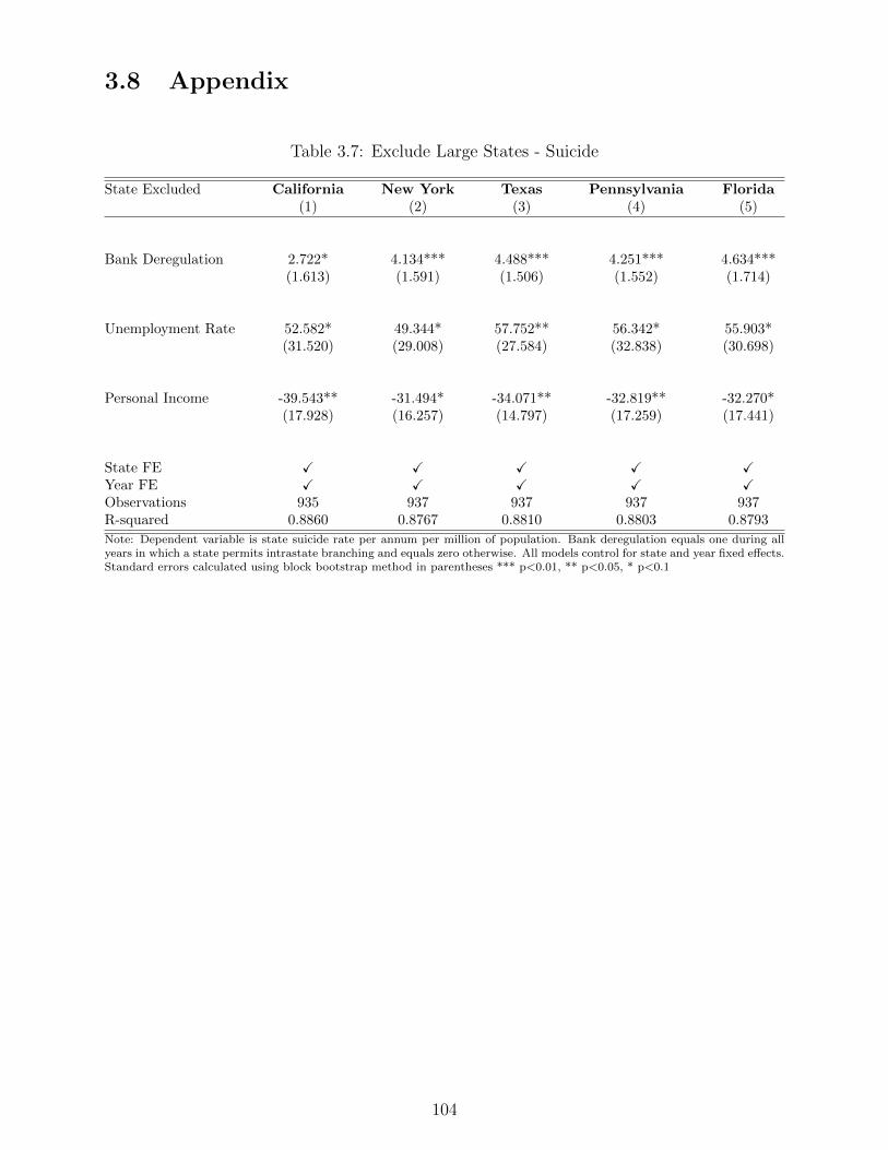
3.8 Appendix

Table 3.7: Exclude Large States - Suicide

State Excluded California New York Texas Pennsylvania Florida(1) (2) (3) (4) (5)

Bank Deregulation 2.722* 4.134*** 4.488*** 4.251*** 4.634***(1.613) (1.591) (1.506) (1.552) (1.714)

Unemployment Rate 52.582* 49.344* 57.752** 56.342* 55.903*(31.520) (29.008) (27.584) (32.838) (30.698)

Personal Income -39.543** -31.494* -34.071** -32.819** -32.270*(17.928) (16.257) (14.797) (17.259) (17.441)

State FE X X X X XYear FE X X X X XObservations 935 937 937 937 937R-squared 0.8860 0.8767 0.8810 0.8803 0.8793

Note: Dependent variable is state suicide rate per annum per million of population. Bank deregulation equals one during allyears in which a state permits intrastate branching and equals zero otherwise. All models control for state and year fixed effects.Standard errors calculated using block bootstrap method in parentheses *** p<0.01, ** p<0.05, * p<0.1

104

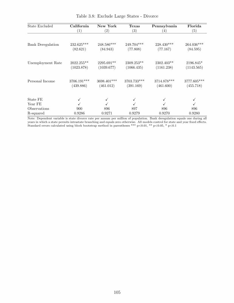
Table 3.8: Exclude Large States - Divorce

State Excluded California New York Texas Pennsylvania Florida(1) (2) (3) (4) (5)

Bank Deregulation 232.625*** 248.586*** 249.704*** 228.430*** 264.036***(82.621) (84.943) (77.808) (77.167) (84.595)

Unemployment Rate 2022.255** 2295.691** 2309.253** 2302.403** 2196.845*(1023.878) (1039.677) (1066.435) (1161.238) (1143.565)

Personal Income 3706.191*** 3698.401*** 3703.733*** 3714.878*** 3777.605***(439.886) (461.012) (391.169) (461.600) (455.718)

State FE X X X X XYear FE X X X X XObservations 900 896 897 896 896R-squared 0.9286 0.9271 0.9279 0.9270 0.9280

Note: Dependent variable is state divorce rate per annum per million of population. Bank deregulation equals one during allyears in which a state permits intrastate branching and equals zero otherwise. All models control for state and year fixed effects.Standard errors calculated using block bootstrap method in parentheses *** p<0.01, ** p<0.05, * p<0.1

105

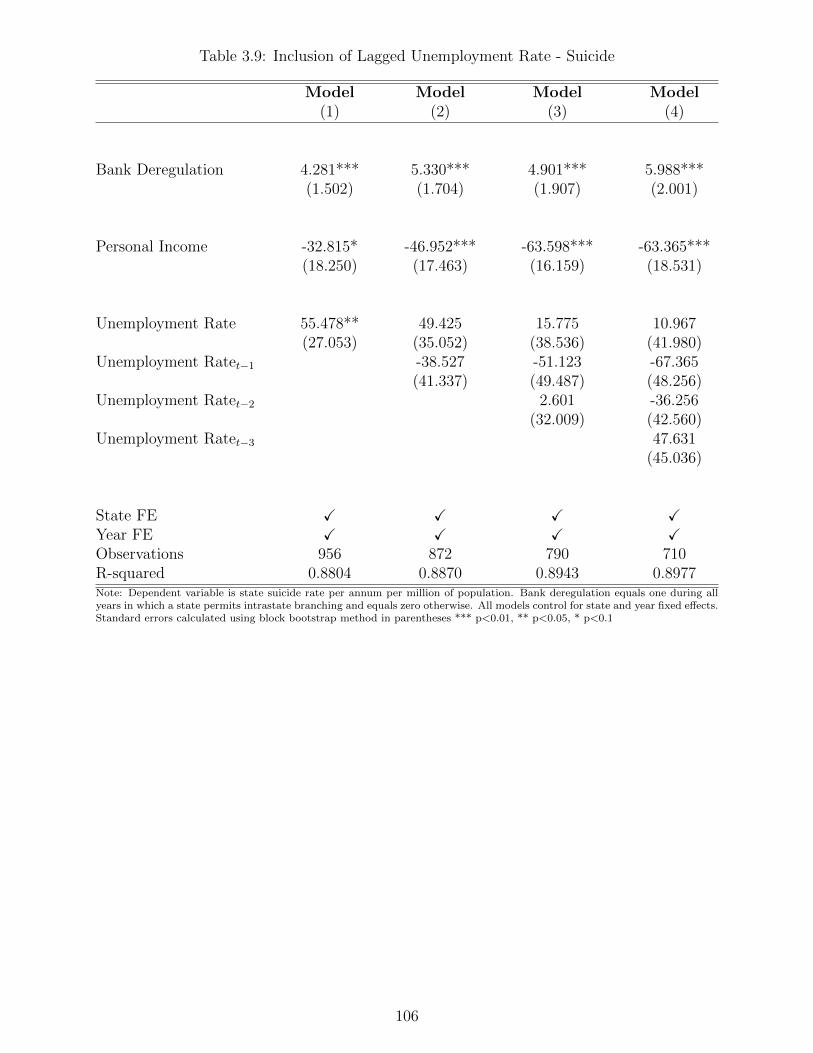
Table 3.9: Inclusion of Lagged Unemployment Rate - Suicide

Model Model Model Model(1) (2) (3) (4)


Personal Income -32.815* -46.952*** -63.598*** -63.365***(18.250) (17.463) (16.159) (18.531)

Unemployment Rate 55.478** 49.425 15.775 10.967(27.053) (35.052) (38.536) (41.980)

Unemployment Ratet−1 -38.527 -51.123 -67.365(41.337) (49.487) (48.256)

Unemployment Ratet−2 2.601 -36.256(32.009) (42.560)

Unemployment Ratet−3 47.631(45.036)

State FE X X X XYear FE X X X XObservations 956 872 790 710R-squared 0.8804 0.8870 0.8943 0.8977Note: Dependent variable is state suicide rate per annum per million of population. Bank deregulation equals one during allyears in which a state permits intrastate branching and equals zero otherwise. All models control for state and year fixed effects.Standard errors calculated using block bootstrap method in parentheses *** p<0.01, ** p<0.05, * p<0.1

106

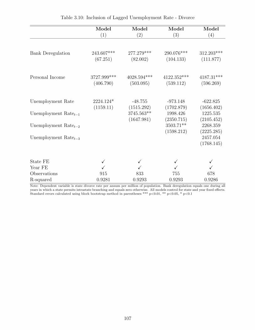
Table 3.10: Inclusion of Lagged Unemployment Rate - Divorce

Model Model Model Model(1) (2) (3) (4)


Personal Income 3727.999*** 4028.594*** 4122.352*** 4187.31***(406.790) (503.095) (539.112) (596.269)

Unemployment Rate 2224.124* -48.755 -973.148 -622.825(1159.11) (1515.292) (1702.879) (1656.402)

Unemployment Ratet−1 3745.563** 1998.426 1225.535(1647.981) (2350.715) (2105.452)

Unemployment Ratet−2 3503.71** 2268.359(1598.212) (2225.285)

Unemployment Ratet−3 2457.054(1768.145)

State FE X X X XYear FE X X X XObservations 915 833 755 678R-squared 0.9281 0.9293 0.9293 0.9286Note: Dependent variable is state divorce rate per annum per million of population. Bank deregulation equals one during allyears in which a state permits intrastate branching and equals zero otherwise. All models control for state and year fixed effects.Standard errors calculated using block bootstrap method in parentheses *** p<0.01, ** p<0.05, * p<0.1

107

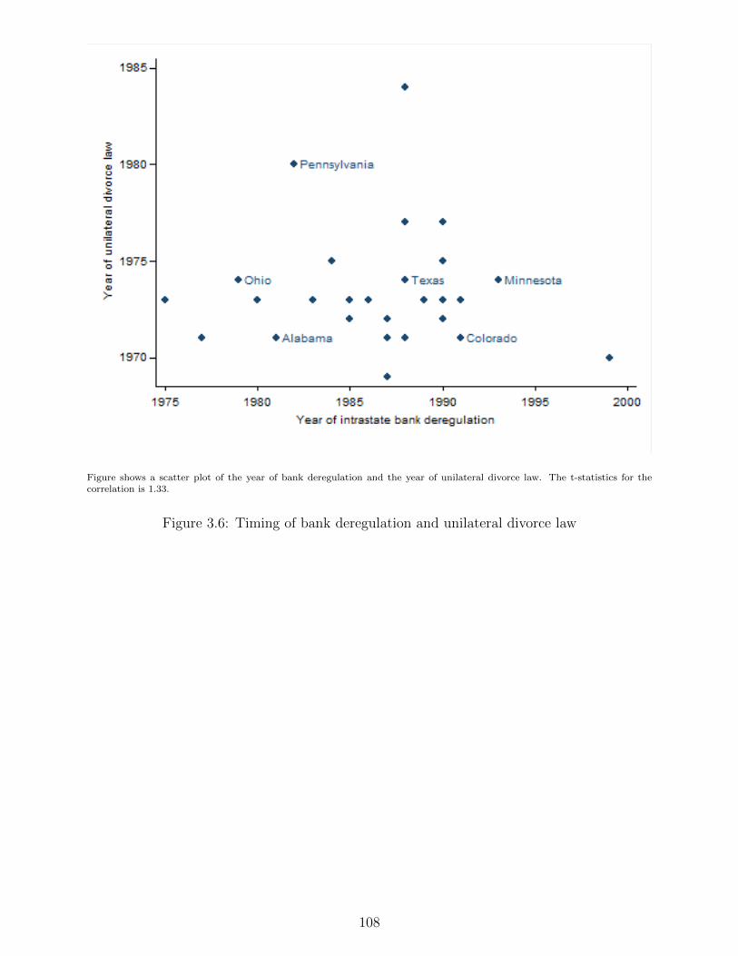
Figure shows a scatter plot of the year of bank deregulation and the year of unilateral divorce law. The t-statistics for thecorrelation is 1.33.

Figure 3.6: Timing of bank deregulation and unilateral divorce law

108

Bibliography

Abiad, A. and Mody, A. (2005). Financial reform: What shakes it? what shapes it?

The American Economic Review, 95(1):66–88.

Acemoglu, D., Johnson, S., and Robinson, J. A. (2001). The colonial origins of

comparative development: An empirical investigation. American economic review,

91(5):1369–1401.

Acemoglu, D., Robinson, J., et al. (2008). The role of institutions in growth and

development. World Bank, Washington DC.

Acemoglu, D. and Robinson, J. A. (2008). Persistence of power, elites, and institu-

tions. American Economic Review, 98(1):267–93.

Alesina, A., Ardagna, S., and Trebbi, F. (2006). Who adjusts and when? on the

political economy of reforms. Technical report, National Bureau of Economic

Research.

Alesina, A. F., Troiano, U., and Cassidy, T. (2015). Old and young politicians.

Technical report, National Bureau of Economic Research.

109

Andersen, J. J. and Aslaksen, S. (2013). Oil and political survival. Journal of

Development Economics, 100(1):89–106.

Angrist, J. D. and Pischke, J.-S. (2008). Mostly harmless econometrics: An empiri-

cist’s companion. Princeton university press.

Arellano, M. and Bond, S. (1991). Some tests of specification for panel data: Monte

carlo evidence and an application to employment equations. The review of eco-

nomic studies, 58(2):277–297.

Bazzi, S. and Blattman, C. (2014). Economic shocks and conflict: Evidence from

commodity prices. American Economic Journal: Macroeconomics, 6(4):1–38.

Beck, T. and Levine, R. (2004). Stock markets, banks, and growth: Panel evidence.

Journal of Banking & Finance, 28(3):423–442.

Beck, T., Levine, R., and Levkov, A. (2010). Big bad banks? the winners and losers

from bank deregulation in the united states. The Journal of Finance, 65(5):1637–

1667.

Beland, L.-P. (2015). Political parties and labor market outcomes: Evidence from

US states. American Economic Journal: Applied Economics, 7(4):198–220.

Bertrand, M., Duflo, E., and Mullainathan, S. (2004). How much should we

trust differences-in-differences estimates? The Quarterly Journal of Economics,

119(1):249–275.

110

Besley, T. and Case, A. (1995). Does electoral accountability affect economic pol-

icy choices? evidence from gubernatorial term limits. The Quarterly Journal of

Economics, 110(3):769–798.

Black, S. E. and Strahan, P. E. (2002). Entrepreneurship and bank credit availability.

The Journal of Finance, 57(6):2807–2833.

Blinder, A. S. and Watson, M. W. (2016). Presidents and the us economy: An

econometric exploration. The American Economic Review, 106(4):1015–1045.

Bond, P., Musto, D. K., and Yilmaz, B. (2009). Predatory mortgage lending. Journal

of Financial Economics, 94(3):412–427.

Bonfiglioli, A. and Gancia, G. A. (2015). Economic uncertainty and structural re-

forms.

Bridges, S. and Disney, R. (2010). Debt and depression. Journal of Health Economics,

29(3):388–403.

Brodeur, A., Le, M., Sangnier, M., and Zylberberg, Y. (2016). Star wars: The

empirics strike back. American Economic Journal: Applied Economics, 8(1):1–32.

Brown, S., Taylor, K., and Price, S. W. (2005). Debt and distress: Evaluating the

psychological cost of credit. Journal of Economic Psychology, 26(5):642–663.

Bruckner, M. and Ciccone, A. (2010). International commodity prices, growth

and the outbreak of civil war in sub-saharan africa. The Economic Journal,

120(544):519–534.

111

Bruckner, M., Ciccone, A., and Tesei, A. (2012). Oil price shocks, income, and

democracy. Review of Economics and Statistics, 94(2):389–399.

Bulanda, J. R. and Brown, S. L. (2007). Race-ethnic differences in marital quality

and divorce. Social Science Research, 36(3):945–967.

Burke, P. J. and Leigh, A. (2010). Do output contractions trigger democratic change?

American Economic Journal: Macroeconomics, 2(4):124–157.

Calderon, C. A., Chong, A., and Loayza, N. V. (2002). Determinants of current

account deficits in developing countries. Contributions in Macroeconomics, 2(1).

Calonico, S., Cattaneo, M. D., and Titiunik, R. (2014). Robust nonparametric con-

fidence intervals for regression-discontinuity designs. Econometrica, 82(6):2295–

2326.

Calonico, S., Cattaneo, M. D., and Titiunik, R. (2015). rdrobust: An r package

for robust nonparametric inference in regression-discontinuity designs. R Journal,

7(1):38–51.

Card, D., Mas, A., Moretti, E., and Saez, E. (2012). Inequality at work: The effect

of peer salaries on job satisfaction. American Economic Review, 102(6):2981–3003.

Caselli, F. and Tesei, A. (2016). Resource windfalls, political regimes, and political

stability. Review of Economics and Statistics, 98(3):573–590.

Cattaneo, M. D., Jansson, M., and Ma, X. (2015). Simple local regression distribution

estimators with an application to manipulation testing. Technical report, working

paper, University of Michigan.

112

Caughey, D., Warshaw, C., and Xu, Y. (2016). Incremental democracy: The pol-

icy effects of the partisan composition of state government. Journal of Politics

(forthcoming).

Chetty, R., Hendren, N., and Katz, L. F. (2016). The effects of exposure to better

neighborhoods on children: New evidence from the moving to opportunity exper-

iment. American Economic Review, 106(4):855–902.

Coope, C., Gunnell, D., Hollingworth, W., Hawton, K., Kapur, N., Fearn, V., Wells,

C., and Metcalfe, C. (2014). Suicide and the 2008 economic recession: who is most

at risk? trends in suicide rates in england and wales 2001–2011. Social Science &

Medicine, 117:76–85.

de Benedictis-Kessner, J. and Warshaw, C. (2016). Mayoral partisanship and mu-

nicipal fiscal policy. The Journal of Politics, 78(4):1124–1138.

de la Cuesta, B. and Imai, K. (2016). Misunderstandings about the regression discon-

tinuity design in the study of close elections. Annual Review of Political Science,

19:375–396.

Deaton, A. (1999). Conmmodity prices and growth in africa. The Journal of Eco-

nomic Perspectives, 13(3):23–40.

Dew, J. (2007). Two sides of the same coin? the differing roles of assets and consumer

debt in marriage. Journal of Family and Economic Issues, 28(1):89–104.

Dew, J., Britt, S., and Huston, S. (2012). Examining the relationship between finan-

cial issues and divorce. Family Relations, 61(4):615–628.

113

Dick, A. A. and Lehnert, A. (2010). Personal bankruptcy and credit market compe-

tition. The Journal of Finance, 65(2):655–686.

Drazen, A. and Easterly, W. (2001). Do crises induce reform? simple empirical tests

of conventional wisdom. Economics & Politics, 13(2):129–157.

Dunning, J. H. (1998). Location and the multinational enterprise: a neglected factor?

Journal of international business studies, 29(1):45–66.

Eggers, A. C., Fowler, A., Hainmueller, J., Hall, A. B., and Snyder, J. M. (2015). On

the validity of the regression discontinuity design for estimating electoral effects:

New evidence from over 40,000 close races. American Journal of Political Science,

59(1):259–274.

Eggers, A. C. and Hainmueller, J. (2009). Mps for sale? returns to office in postwar

british politics. American Political Science Review, 103(04):513–533.

Erikson, R. S., Folke, O., and Snyder Jr, J. M. (2015). A gubernatorial helping hand?

how governors affect presidential elections. The Journal of Politics, 77(2):491–504.

Faccio, M. (2006). Politically connected firms. American economic review, 96(1):369–

386.

Fan, J. and Gijbels, I. (1996). Local polynomial modelling and its applications: mono-

graphs on statistics and applied probability 66, volume 66. CRC Press.

Fernandez, R. and Rodrik, D. (1991). Resistance to reform: Status quo bias in the

presence of individual-specific uncertainty. The American Economic Review, pages

1146–1155.

114

Ferreira, F., Gyourko, J., et al. (2009). Do political parties matter? evidence from

us cities. The Quarterly Journal of Economics, 124(1):399–422.

Fitch, C., Chaplin, R., Trend, C., and Collard, S. (2007). Debt and mental health:

the role of psychiatrists. Advances in Psychiatric Treatment, 13(3):194–202.

Fox, G. L., Benson, M. L., DeMaris, A. A., and Wyk, J. (2002). Economic distress

and intimate violence: Testing family stress and resources theories. Journal of

Marriage and Family, 64(3):793–807.

Fox, S. E. (1996). The influence of political conditions on foreign firm location deci-

sions in the american states (1974-1989). Political Research Quarterly, 49(1):51–75.

Frasquilho, D., Matos, M. G., Salonna, F., Guerreiro, D., Storti, C. C., Gaspar,

T., and Caldas-de Almeida, J. M. (2015). Mental health outcomes in times of

economic recession: a systematic literature review. BMC public health, 16(1):115.

Friedberg, L. (1998). Did unilateral divorce raise divorce rates? evidence from panel

data. The American Economic Review, 88(3):608–627.

Fry, E. H. (1998). The expanding role of state and local governments in US foreign

affairs. New York (USA) Council on Foreign Relations Press.

Garmaise, M. J. and Moskowitz, T. J. (2006). Bank mergers and crime: The real and

social effects of credit market competition. The Journal of Finance, 61(2):495–538.

Gathergood, J. (2011). Debt and depression: Evidence on causal links and social

stigma effects.

115

Gathergood, J. (2012). Self-control, financial literacy and consumer over-

indebtedness. Journal of Economic Psychology, 33(3):590–602.

Gelman, A. and Imbens, G. (2014). Why high-order polynomials should not be used

in regression discontinuity designs. Technical report, National Bureau of Economic

Research.

Gerber, E. R. and Hopkins, D. J. (2011). When mayors matter: estimating the impact

of mayoral partisanship on city policy. American Journal of Political Science,

55(2):326–339.

Giuliano, P., Mishra, P., and Spilimbergo, A. (2013). Democracy and reforms:

evidence from a new dataset. American Economic Journal: Macroeconomics,

5(4):179–204.

Grable, J. E., Britt, S., and Cantrell, J. (2007). An exploratory study of the role

financial satisfaction has on the thought of subsequent divorce. Family and Con-

sumer Sciences Research Journal, 36(2):130–150.

Grimmer, J., Hersh, E., Feinstein, B., and Carpenter, D. (2011). Are close elections

random? Unpublished manuscript.

Grossman, G. M. and Helpman, E. (2001). Special interest politics. MIT press.

Gunnell, D., Donovan, J., Barnes, M., Davies, R., Hawton, K., Kapur, N., Holling-

worth, W., and Metcalfe, C. (1998). The 2008 global financial crisis: effects on

mental health and suicide. Age, 2003(2008):2013.

116

Halvorsen, T. and Jakobsen, J. (2013). Democrats, republicans or both? an empirical

analysis of the effects of the composition of state governments on fdi, 1977–2004.

International Interactions, 39(2):167–191.

Hansen, S. (1989). The Political Economy of State Industrial Policy. University of

Pittsburgh Press.

Hatcher, S. (1994). Debt and deliberate self-poisoning. The British Journal of Psy-

chiatry, 164(1):111–114.

Head, C. K., Ries, J. C., and Swenson, D. L. (1999). Attracting foreign manufac-

turing: Investment promotion and agglomeration. Regional Science and Urban

Economics, 29(2):197–218.

Hintikka, J., Kontula, O., Saarinen, P., Tanskanen, A., Koskela, K., and Viinamaki,

H. (1998). Debt and suicidal behaviour in the finnish general population. Acta

Psychiatrica Scandinavica, 98(6):493–496.

Høj, J., Galasso, V., Nicoletti, G., and Dang, T.-T. (2006). The political economy

of structural reform.

Imbens, G. and Kalyanaraman, K. (2011). Optimal bandwidth choice for the regres-

sion discontinuity estimator. The Review of Economic Studies, page rdr043.

Imbens, G. W. and Wooldridge, J. M. (2009). Recent developments in the econo-

metrics of program evaluation. Journal of Economic Literature, 47(1):5–86.

Innes, R. and Mitra, A. (2015). Parties, politics, and regulation: Evidence from clean

air act enforcement. Economic Inquiry, 53(1):522–539.

117

Jayaratne, J. and Strahan, P. E. (1996). The finance-growth nexus: Evidence from

bank branch deregulation. The Quarterly Journal of Economics, 111(3):639–670.

Jayaratne, J. and Strahan, P. E. (1998). Entry restrictions, industry evolution, and

dynamic efficiency: Evidence from commercial banking. The Journal of Law and

Economics, 41(1):239–274.

Klasnja, M. and Titiunik, R. (2014). The incumbency curse: Weak parties, term

limits, and unfulfilled accountability. American Political Science Review.

Kroszner, R. S. and Strahan, P. E. (1999). What drives deregulation? economics and

politics of the relaxation of bank branching restrictions. The Quarterly Journal of

Economics, 114(4):1437–1467.

Kubrin, C. E. and Wadsworth, T. (2009). Explaining suicide among blacks and

whites: How socioeconomic factors and gun availability affect race-specific suicide

rates. Social Science Quarterly, 90(5):1203–1227.

Lee, D. S. (2008). Randomized experiments from non-random selection in us house

elections. Journal of Econometrics, 142(2):675–697.

Lee, D. S. and Lemieux, T. (2010). Regression discontinuity designs in economics.

Journal of Economic Literature, 48(2):281–355.

Lee, D. S., Moretti, E., and Butler, M. J. (2004). Do voters affect or elect policies?

evidence from the us house. The Quarterly Journal of Economics, 119(3):807–859.

118

Leigh, A. (2008). Estimating the impact of gubernatorial partisanship on policy

settings and economic outcomes: A regression discontinuity approach. European

Journal of Political Economy, 24(1):256–268.

Leip, D. (2008). Atlas of US Presidential Elections. Online document:

http://www.uselectionatlas.org.

List, J. A. and Sturm, D. M. (2006). How elections matter: Theory and evidence from

environmental policy. The Quarterly Journal of Economics, 121(4):1249–1281.

McCrary, J. (2008). Manipulation of the running variable in the regression disconti-

nuity design: A density test. Journal of Econometrics, 142(2):698–714.

McMillan, S. L. (2009). Looking beyond the national level: foreign direct investment

attraction in us states. International Interactions, 35(2):155–178.

Melzer, B. T. (2011). The real costs of credit access: Evidence from the payday

lending market. The Quarterly Journal of Economics, 126(1):517–555.

Merriott, D. (2016). Factors associated with the farmer suicide crisis in india. Journal

of Epidemiology and Global Health, 6(4):217–227.

Mian, A., Sufi, A., and Trebbi, F. (2014). Resolving debt overhang: political con-

straints in the aftermath of financial crises. American Economic Journal: Macroe-

conomics, 6(2):1–28.

Michael, R. T. (1978). The rise in divorce rates, 1960–1974: Age-specific components.

Demography, 15(2):177–182.

119

Nickell, S. (1981). Biases in dynamic models with fixed effects. Econometrica: Jour-

nal of the Econometric Society, pages 1417–1426.

Office of Trade and Economic Analysis (2016). Jobs attributable to foreign direct

investment in the united states.

Papp, L. M., Cummings, E. M., and Goeke-Morey, M. C. (2009). For richer, for

poorer: Money as a topic of marital conflict in the home. Family Relations,

58(1):91–103.

Persson, T. and Tabellini, G. (2006). Democratic capital: The nexus of political and

economic change. Technical report, National Bureau of Economic Research.

Pinto, P. M. and Pinto, S. M. (2008). The politics of investment partisanship:

And the sectoral allocation of foreign direct investment. Economics & Politics,

20(2):216–254.

Prati, A., Onorato, M. G., and Papageorgiou, C. (2013). Which reforms work and

under what institutional environment? evidence from a new data set on structural

reforms. Review of Economics and Statistics, 95(3):946–968.

Preti, A. and Miotto, P. (1998). Seasonality in suicides: the influence of suicide

method, gender and age on suicide distribution in italy. Psychiatry research,

81(2):219–231.

Quinn, D. P. and Shapiro, R. Y. (1991). Economic growth strategies: The effects

of ideological partisanship on interest rates and business taxation in the united

states. American Journal of Political Science, pages 656–685.

120

Ranciere, R. G. and Tornell, A. (2016). Why do reforms occur in crises times?

Reading, R. and Reynolds, S. (2001). Debt, social disadvantage and maternal de-

pression. Social Science & Medicine, 53(4):441–453.

Reed, W. R. (2006). Democrats, republicans, and taxes: Evidence that political

parties matter. Journal of Public Economics, 90(4):725–750.

Resmini, L. (2000). The determinants of foreign direct investment in the ceecs: New

evidence from sectoral patterns. Economics of transition, 8(3):665–689.

Roodman, D. (2009). A note on the theme of too many instruments. Oxford Bulletin

of Economics and statistics, 71(1):135–158.

Skovron, C. and Titiunik, R. (2015). A practical guide to regression discontinuity

designs in political science. American Journal of Political Science.

Snowberg, E., Wolfers, J., and Zitzewitz, E. (2007). Partisan impacts on the economy:

Evidence from prediction markets and close elections. The Quarterly Journal of

Economics, 122(2):807–829.

Stevenson, B. and Wolfers, J. (2006). Bargaining in the shadow of the law: Divorce

laws and family distress. The Quarterly Journal of Economics, 121(1):267–288.

Sun, S. T. and Yannelis, C. (2016). Credit constraints and demand for higher edu-

cation: Evidence from financial deregulation. Review of Economics and Statistics,

98(1):12–24.

121

Tewari, I. (2014). The distributive impacts of financial development: Evidence from

mortgage markets during us bank branch deregulation. American Economic Jour-

nal: Applied Economics, 6(4):175–96.

Thistlethwaite, D. L. and Campbell, D. T. (1960). Regression-discontinuity analysis:

An alternative to the ex post facto experiment. Journal of Educational Psychology,

51(6):309.

Tommasi, M. and Velasco, A. (1996). Where are we in the political economy of

reform? The Journal of Policy Reform, 1(2):187–238.

Watson, D. J. (1995). The new civil war: government competition for economic

development. Praeger Publishers.

Whatley, C. (2003). State official’s guide to international affairs. Council of State

Governments.

Wheeler, D. and Mody, A. (1992). International investment location decisions: The

case of us firms. Journal of international economics, 33(1-2):57–76.

Yip, P. S., Yang, K. C., Ip, B. Y., Law, Y., and Watson, R. (2007). Financial debt and

suicide in hong kong sar. Journal of Applied Social Psychology, 37(12):2788–2799.

Yu, J. and Walsh, M. J. P. (2010). Determinants of foreign direct investment: A

sectoral and institutional approach. Number 10-187. International Monetary Fund.

122

Documents

Essays in Applied Economics - University of Ottawa