Embed Size (px)
Citation preview

ESCI 386 – Scientific Programming, Analysis and Visualization with
Python
Lesson 17 - Fourier Transforms
1

Spectral Analysis
• Most any signal can be decomposed into a sum of sine and cosine waves of various amplitudes and wavelengths.
2
Fourier Coefficients
• For each frequency of wave contained in the signal there is a complex-valued Fourier coefficient.
• The real part of the coefficient contains information about the amplitude of the cosine waves
• The imaginary part of the coefficient contains information about the amplitude of the sine waves
3

Discrete Fourier Transform (DFT)
• The discrete Fourier transform pair
• N is number of data points
4
1
0
( ) ( )exp 2N
m
f n F m i mn N
1
0
1( ) ( )exp 2
N
n
F m f n i mn NN
Forward transform
Backward or inverse transform

Discrete Fourier Transforms
• f (n) is value of function f at grid point n.
• F(m) is the spectral coefficient for the mth wave component.
5
1
0
( ) ( )exp 2N
m
f n F m i mn N
1
0
1( ) ( )exp 2
N
n
F m f n i mn NN

Discrete Fourier Transforms
• f (n) may be real or complex-valued.
• F(m) is always complex-valued.
6
1
0
( ) ( )exp 2N
m
f n F m i mn N
1
0
1( ) ( )exp 2
N
n
F m f n i mn NN

DFT • There will be as many Fourier coefficients (waves)
as there are grid points.
• The natural frequencies/wave numbers associated with the Fourier coefficients are
7
; 0,1,2, , 2
1; 2 1, 2 2, 2 3, , 2
m
s
m
s
mm N
N
N mm N N N N N
N
for negative frequencies
for positive frequencies

The Frequencies/Wave Numbers
• If the input function f(n) is entirely real then the negative frequencies are completely redundant, giving no additional information.
• The highest natural frequency (wave number) that can be represented in a digital signal is called the Nyquist frequency, and is given as 1/2 where is the sampling interval/period.
8

The zeroth Coefficient
• The zeroth Fourier coefficient is the average value of the signal over the interval.
9

Show Visualizations
10
Power Spectrum
• The Fourier coefficients, F(m), are complex numbers, containing a real part and an imaginary part.
• The real part corresponds to the cosine waves that make up the function (the even part of the original function), and the negative of the imaginary terms correspond to the sine waves (the odd part of the original function).
11
Power Spectrum
• For a sinusoid that has an integer number of cycles within the N data points, the amplitude of the sine or cosine wave is twice its Fourier coefficient. – So, a pure cosine wave of amplitude one would have a
single real Fourier coefficient at its frequency, and the value of that coefficient would be 0.5.
• The magnitude squared of the Fourier coefficients , |F(m)|2 , is called the power. – A plot of the power vs. frequency is referred to as the
power spectrum.
12

Power Spectra for Square Signal
13

Power Spectra for Gaussian Signal
14
The numpy.fft Module
15
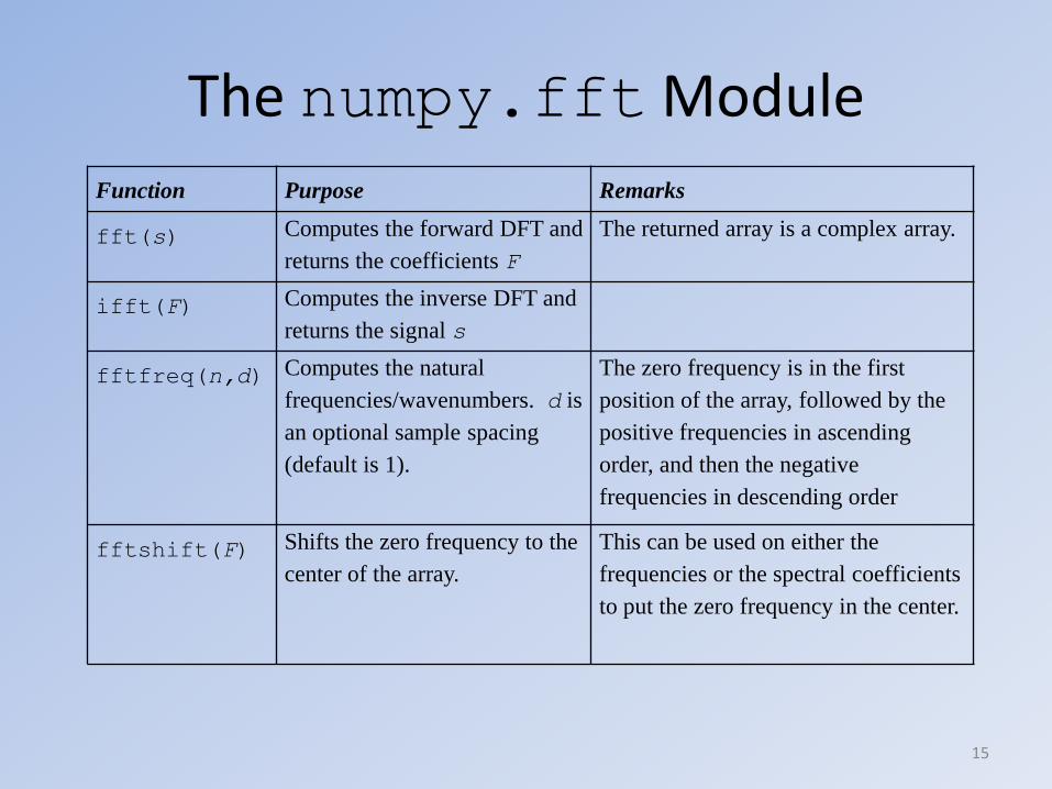
Function Purpose Remarks
fft(s) Computes the forward DFT and
returns the coefficients F
The returned array is a complex array.
ifft(F) Computes the inverse DFT and
returns the signal s
fftfreq(n,d) Computes the natural
frequencies/wavenumbers. d is
an optional sample spacing
(default is 1).
The zero frequency is in the first
position of the array, followed by the
positive frequencies in ascending
order, and then the negative
frequencies in descending order
fftshift(F) Shifts the zero frequency to the
center of the array.
This can be used on either the
frequencies or the spectral coefficients
to put the zero frequency in the center.

The numpy.fft Module (cont.)
• There are also functions for taking FFTs in two or more dimensions, and for taking FFTs of purely real signals and returning only the positive coefficients. See documentation for details.
• We normally import this as
from numpy import fft
16
The numpy.fft.fft() Function
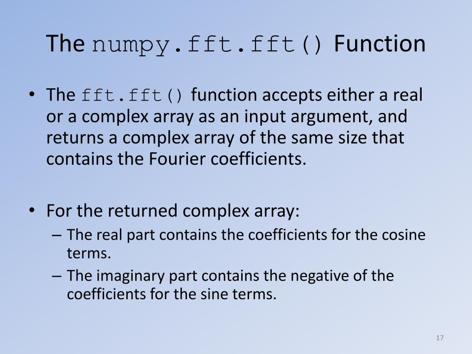
• The fft.fft() function accepts either a real or a complex array as an input argument, and returns a complex array of the same size that contains the Fourier coefficients.
• For the returned complex array: – The real part contains the coefficients for the cosine
terms.
– The imaginary part contains the negative of the coefficients for the sine terms.
17

The fft.fft() Function (cont.)
• IMPORTANT NOTICE!!! There are different definitions for how a DFT should be taken.
18
The fft.fft() Function (cont.)
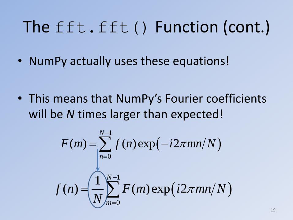
• NumPy actually uses these equations!
• This means that NumPy’s Fourier coefficients will be N times larger than expected!
19
1
0
1( ) ( )exp 2
N
m
f n F m i mn NN
1
0
( ) ( )exp 2N
n
F m f n i mn N

The fft.fftfreq() Function
• The natural frequencies associated with the spectral coefficients are calculated using the fft.fft() function.
• The zeroth frequency is first, followed by the positive frequencies in ascending order, and then the negative frequencies in descending order.
20

FFT Example Program from numpy import fft
import numpy as np
import matplotlib.pyplot as plt
n = 1000 # Number of data points
dx = 5.0 # Sampling period (in meters)
x = dx*np.arange(0,n) # x coordinates
w1 = 100.0 # wavelength (meters)
w2 = 20.0 # wavelength (meters)
fx = np.sin(2*np.pi*x/w1) + 2*np.cos(2*np.pi*x/w2) # signal
Fk = fft.fft(fx)/n # Fourier coefficients (divided by n)
nu = fft.fftfreq(n,dx) # Natural frequencies
Fk = fft.fftshift(Fk) # Shift zero freq to center
nu = fft.fftshift(nu) # Shift zero freq to center
f, ax = plt.subplots(3,1,sharex=True)
ax[0].plot(nu, np.real(Fk)) # Plot Cosine terms
ax[0].set_ylabel(r'$Re[F_k]$', size = 'x-large')
ax[1].plot(nu, np.imag(Fk)) # Plot Sine terms
ax[1].set_ylabel(r'$Im[F_k]$', size = 'x-large')
ax[2].plot(nu, np.absolute(Fk)**2) # Plot spectral power
ax[2].set_ylabel(r'$\vert F_k \vert ^2$', size = 'x-large')
ax[2].set_xlabel(r'$\widetilde{\nu}$', size = 'x-large')
plt.show()
21 File: fft-example.py
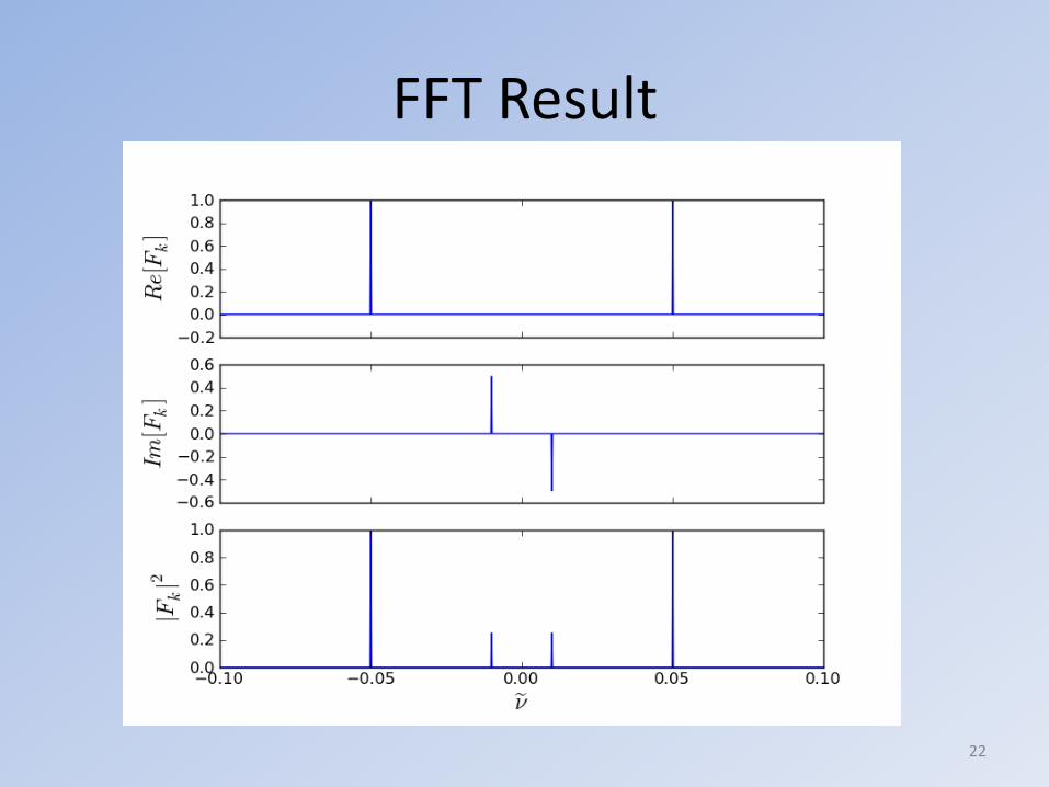
FFT Result
22

FFT Leakage
• There are no limits on the number of data points when taking FFTs in NumPy.
• The FFT algorithm is much more efficient if the number of data points is a power of 2 (128, 512, 1024, etc.).
• The DFT assumes that the signal is periodic on the interval 0 to N, where N is the total number of data points in the signal.
• Care needs to be taken to ensure that all waves in the signal are periodic within the interval 0 to N, or a phenomenon known as leakage will occur.
23
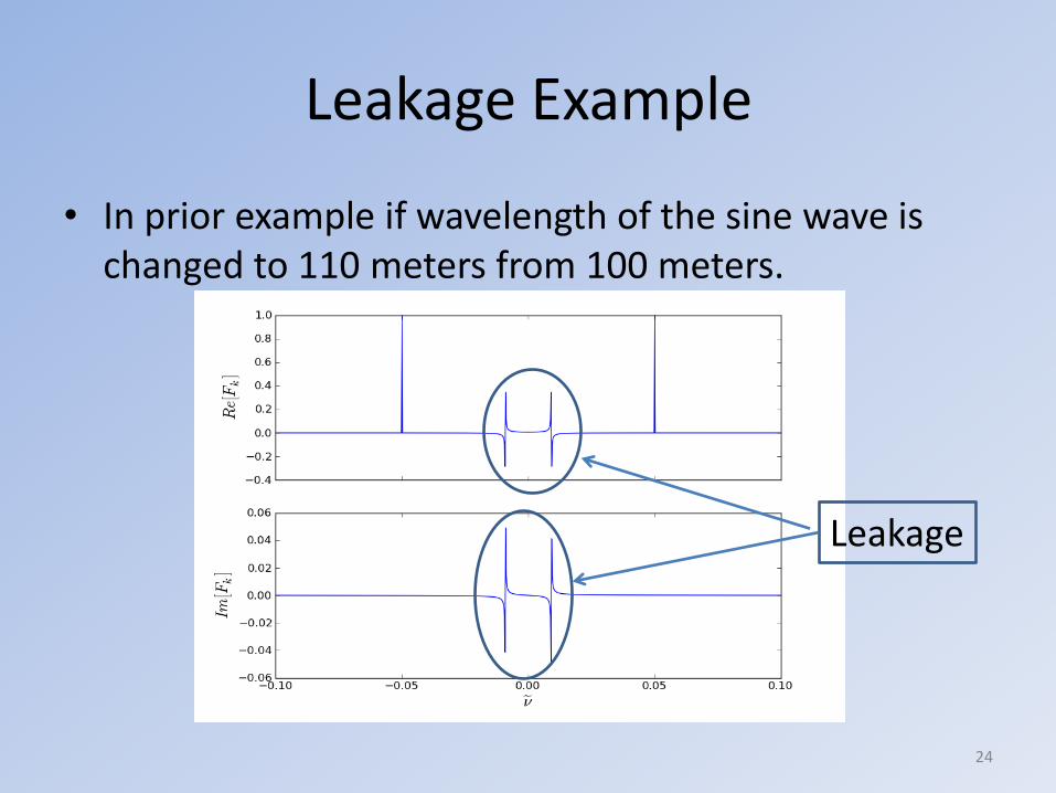
Leakage Example
• In prior example if wavelength of the sine wave is changed to 110 meters from 100 meters.
24
Leakage
The fft.rfft() Function
• Since for real input the negative frequencies are redundant, there is an fft.rfft() function that only computes the positive coefficients for a real input.
• The helper routine fftfreq() only returns the frequencies for the complex FFT.
25
The fft.rfft() Function
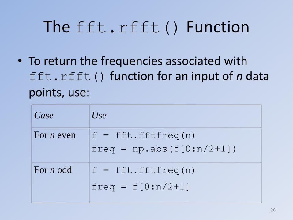
• To return the frequencies associated with fft.rfft() function for an input of n data points, use:
26
Case Use
For n even f = fft.fftfreq(n)
freq = np.abs(f[0:n/2+1])
For n odd f = fft.fftfreq(n)
freq = f[0:n/2+1]