ESA Standard Document

ESA UNCLASSIFIED – For Official Use

esrin Via Galileo Galilei

Casella Postale 64 00044 Frascati

Italy T +39 06 9418 01

F +39 06 9418 0280 www.esa.int

Guidelines for the SAR (Delay-Doppler) L1b Processing

Prepared by Salvatore Dinardo Reference XCRY-GSEG-EOPS-TN-14-0042 Issue 2 Revision 3 Date of Issue 29/05/2013 Status Approved/Applicable Document Type TN Distribution


Title Guidelines for the SAR (Delay-Doppler) L1b Processing

Issue 2 Revision 3

Author Salvatore Dinardo Date 29/05/2013

Approved by Jerome Benveniste Date 29/05/2013

Reason for change Issue Revision Date

Issue 2 Revision 3 Reason for change Date Pages Paragraph(s)

Page 2/20 Date 29/05/2013 Issue 2 Rev 3


Table of contents:

REFERENCES & APPLICABLE DOCUMENTS ......................................................................................... 4 1 INTRODUCTION ............................................................................................................................. 5 2 ACRONYMS & GLOSSARY .............................................................................................................. 5 3 CLOSED-BURST DELAY-DOPPLER RADAR ALTIMETER ................................................................ 6 4 SAR (DELAY-DOPPLER) L1B PROCESSING .................................................................................... 6 4.1 Calibration Correction ....................................................................................................................................................... 6 4.2 Ground Cell Gridding ......................................................................................................................................................... 7 4.3 Beam Pointing .................................................................................................................................................................... 7 4.4 Beam Steering & Beam Forming .......................................................................................................................................8 4.4.1 Approximated Beam Steering ........................................................................................................................................ 11 4.4.2 Exact Beam Steering ....................................................................................................................................................... 11 4.5 Beam Stacking .................................................................................................................................................................. 13 4.6 Range Alignment .............................................................................................................................................................. 14 4.6.1 Slant Range Correction .................................................................................................................................................. 14 4.6.2 Tracker Range Correction ............................................................................................................................................. 15 4.6.3 Doppler Range Correction ............................................................................................................................................. 15 4.7 Range Compression ......................................................................................................................................................... 16 4.8 Multi-Looking .................................................................................................................................................................. 17 4.9 Delay-Doppler Processing Block-Scheme ....................................................................................................................... 19 4.10 CryoSat-2 and Sentinel-3 L1b SAR Processing Configuration ....................................................................................... 19 5 AKNOWLEDGEMENTS ................................................................................................................. 20



REFERENCES & APPLICABLE DOCUMENTS

[RD1]: CryoSat Product Handbook. April 2012. ESA and Mullard Space Science Laboratory – University College London, (available at http://emits.esa.int/emits-doc/ESRIN/7158/CryoSat-PHB-17apr2012.pdf) [RD2]: Francis, C. R., 2007, “Mission and Data Description”, ESA editor, CS-RP-ESA-SY-0059, issue 3. (available at http://esamultimedia.esa.int/docs/Cryosat/Mission_and_Data_Descrip.pdf) [RD3]: Cullen, R. A., Wingham, D. et al., ESA’s CryoSat-2 Multi-Mode Level 0 to Level 1b Science Processors–Algorithm Design and Pre-Launch Verification with ASIRAS, Envisat Symposium 2007 (available at https://earth.esa.int/envisatsymposium/proceedings/posters/4P4/459065rc.pdf). [RD4]: Cullen, R. A. and Wingham, D. J. , CryoSat level 1b processing algorithms and simulation results. In Geoscience and Remote Sensing Symposium, 2002. IGARSS ’02. 2002 IEEE International, volume 3, pages 1762–1764. Centre for Polar Obs. & Modelling, Univ. Coll. London, UK, IEEE [RD5]: Raney, R. K., 1998, “The Delay/Doppler Radar Altimeter”, IEEE Trans. Geoscience and Remote Sensing, Vol. 36, No. 5, pp. 1578-1588 Sept 1998 [RD6]: Raney, R.K. , 2008, “The Delay-Doppler Altimeter”, in 2nd Coastal Altimetry Workshop, Pisa, Italy, November 2008 [RD6]: Rosmorduc V. and al. Radar Altimetry Tutorial (RAT), February 2011, ESA-CNES/CLS, J. Benveniste & N.Picot Editors, (available at http://www.altimetry.info/documents/Radar_Altimetry_Tutorial_20110216.pdf) [RD7]: ENVISAT RA2/MWR Product Handbook, ESA-ESRIN, Issue 2.2, (available at https://earth.esa.int/handbooks/ra2-mwr/CNTR.htm) [RD8]: Dinardo. S, Waveform Re-tracking starting from Level 2 SGDR DATA, ESA/ESRIN/EOP-SER, issue 1.0, January 2009, (available at http://earth.esa.int/raies/docs/RETR_SGDR.pdf)

Page 4/20 ESA Standard Document Date 29/05/2013 Issue 2 Rev 3

http://emits.esa.int/emits-doc/ESRIN/7158/CryoSat-PHB-17apr2012.pdf

http://emits.esa.int/emits-doc/ESRIN/7158/CryoSat-PHB-17apr2012.pdf

http://esamultimedia.esa.int/docs/Cryosat/Mission_and_Data_Descrip.pdf

https://earth.esa.int/envisatsymposium/proceedings/posters/4P4/459065rc.pdf

http://www.altimetry.info/documents/Radar_Altimetry_Tutorial_20110216.pdf

https://earth.esa.int/handbooks/ra2-mwr/CNTR.htm

http://earth.esa.int/raies/docs/RETR_SGDR.pdf


1 INTRODUCTION

The purpose of this document is to present the major theoretical guidelines for a standard SAR (aka Delay Doppler) Processing from low-level data (FBR, aka L1a) to multi-looked waveforms (L1b) in case of the Closed-Burst instrument transmission mode (CryoSat-2 and Sentinel-3 case). The description does not intend to be comprehensive and fully detailed as it simply aims to give a clear high-level overview of the technical processes which the altimetric signal undergoes during a standard SAR Processing and to shed a light on some particular expressions used in the Delay-Doppler terminology or jargon. The target reader of the present Technical Note is meant to be a conventional altimetry skilled user, holding already all the pulse-limited altimetry theoretical basic principles but eager to extend own knowledge to SAR (Delay-Doppler) concepts. For any instrumental detail on the CryoSat-2 Altimeter working principles and operations in SAR mode, the reader can refer to the CryoSat Handbook [RD1].

2 ACRONYMS & GLOSSARY

Along-Track Direction: direction parallel to the flight direction Across-Track Direction: direction perpendicular to the flight direction AGC: Automatic Gain Control Burst: A series of transmitted radar pulses in sequence COM: Center of Mass Doppler Axis (or zero-Doppler Axis): Axis orthogonal to the satellite velocity vector in the plane holding the velocity vector and geodetic nadir Doppler Beam: Synthetic Antenna Beam, focused exploiting the Doppler shift due to the relative platform motion with respect the ground. The Doppler Beams are more sharpened than the Real Antenna Beam. Doppler Beam Angle: Angle that Doppler Beam Boresight makes with the velocity vector FBR: Full Bit Rate: Un-calibrated Complex (I and Q) Individual Echoes posted at full PRF rate and deramped in time domain FFT: Fast Fourier Transform L1a: Level 1a L1b: Level 1b LPF: Low Pass Filter LPF: Low Pass Filter PRF: Pulse Repetition Frequency Posting Rate: Temporal Rate (Hz) at which the measurement record is posted in a data product



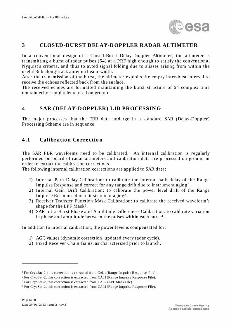
3 CLOSED-BURST DELAY-DOPPLER RADAR ALTIMETER

In a conventional design of a Closed-Burst Delay-Doppler Altimeter, the altimeter is transmitting a burst of radar pulses (64) at a PRF high enough to satisfy the conventional Nyquist’s criteria, and thus to avoid signal folding due to aliases arising from within the useful 3db along-track antenna beam-width. After the transmission of the burst, the altimeter exploits the empty inter-bust interval to receive the echoes reflected back from the surface. The received echoes are formatted maintaining the burst structure of 64 complex time domain echoes and telemetered on ground.

4 SAR (DELAY-DOPPLER) L1B PROCESSING

The major processes that the FBR data undergo in a standard SAR (Delay-Doppler) Processing Scheme are in sequence:

4.1 Calibration Correction The SAR FBR waveforms need to be calibrated. An internal calibration is regularly performed on-board of radar altimeters and calibration data are processed on-ground in order to extract the calibration corrections. The following internal calibration corrections are applied to SAR data:

1) Internal Path Delay Calibration: to calibrate the internal path delay of the Range Impulse Response and correct for any range drift due to instrument aging 1.

2) Internal Gain Drift Calibration: to calibrate the power level drift of the Range Impulse Response due to instrument aging2.

3) Receiver Transfer Function Mask Calibration: to calibrate the received waveform’s shape for the LPF Mask3.

4) SAR Intra-Burst Phase and Amplitude Differences Calibration: to calibrate variation in phase and amplitude between the pulses within each burst4.

In addition to internal calibration, the power level is compensated for:

1) AGC values (dynamic correction, updated every radar cycle). 2) Fixed Receiver Chain Gains, as characterized prior to launch.

1 For CryoSat-2, this correction is extracted from CAL1 (Range Impulse Response File). 2 For CryoSat-2, this correction is extracted from CAL1 (Range Impulse Response File). 3 For CryoSat-2, this correction is extracted from CAL2 (LPF Mask File). 4 For CryoSat-2, this correction is extracted from CAL1 (Range Impulse Response File).



4.2 Ground Cell Gridding The purpose of this stage is to identify along the over-flown surface elevation profile a set of surface locations (or surface samples or ground cells or reference points or Doppler Bins) wherein the synthetized Doppler Beams will be afterwards focused, steered and incoherently accumulated. The position of the surface locations is determined using an iterative method consisting in enforcing between the surface samples the same along-track angular separation, (in order to obtain a regular angular grid) and placing the surface samples on the sub-satellite elevation profile. The along-track angular separation between surface samples is fixed equal to the one by which the Doppler beams are in average separated. The used approximated over-flown elevation profile is derived from the on-board calculated tracker range converted to a surface elevation. Each surface sample is assigned a time-tag equal to the time, in TAI, the satellite passes ellipsoidally normal to the sample. The level 1b multi-looked waveforms will be then time-referenced to these surface sample time-tags and no longer dependent on the burst structure of the input FBR data. This means that the posting rates of the FBR and Level 1b data are independent of each other.

4.3 Beam Pointing Given the set of surface sample locations, the purpose of this stage is to determine for each burst center:

1) vectors joining the position of the current burst center to the positions of the all surface samples (beam direction vectors).

2) the angles between beam direction vectors and satellite velocity vector evaluated in the burst center (beam direction angles).

3) the ranges between the position of satellite COM at burst center and the positions of all the surface samples (beam direction ranges).

Based on all the calculated direction angles, only the surface samples5, whose beam directions are included in the antenna’s physical 3db along-track aperture, are selected and retained in memory.

5 For geometrical reasons, the number of surface samples in the antenna’s physical 3db along-track aperture is variable along the orbit; for software memory size issues, the max accepted number is limited to 64.



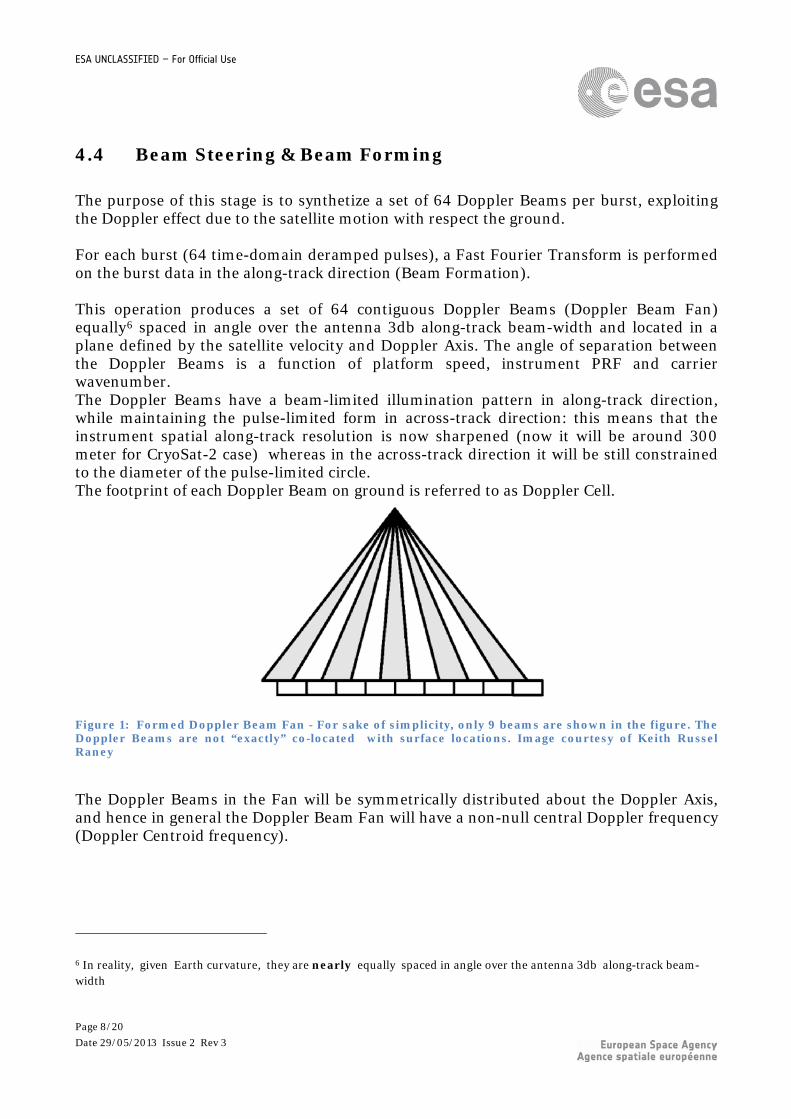
4.4 Beam Steering & Beam Forming The purpose of this stage is to synthetize a set of 64 Doppler Beams per burst, exploiting the Doppler effect due to the satellite motion with respect the ground. For each burst (64 time-domain deramped pulses), a Fast Fourier Transform is performed on the burst data in the along-track direction (Beam Formation). This operation produces a set of 64 contiguous Doppler Beams (Doppler Beam Fan) equally6 spaced in angle over the antenna 3db along-track beam-width and located in a plane defined by the satellite velocity and Doppler Axis. The angle of separation between the Doppler Beams is a function of platform speed, instrument PRF and carrier wavenumber. The Doppler Beams have a beam-limited illumination pattern in along-track direction, while maintaining the pulse-limited form in across-track direction: this means that the instrument spatial along-track resolution is now sharpened (now it will be around 300 meter for CryoSat-2 case) whereas in the across-track direction it will be still constrained to the diameter of the pulse-limited circle. The footprint of each Doppler Beam on ground is referred to as Doppler Cell.

Figure 1: Formed Doppler Beam Fan - For sake of simplicity, only 9 beams are shown in the figure. The Doppler Beams are not “exactly” co-located with surface locations. Image courtesy of Keith Russel Raney

The Doppler Beams in the Fan will be symmetrically distributed about the Doppler Axis, and hence in general the Doppler Beam Fan will have a non-null central Doppler frequency (Doppler Centroid frequency).

6 In reality, given Earth curvature, they are nearly equally spaced in angle over the antenna 3db along-track beam-width



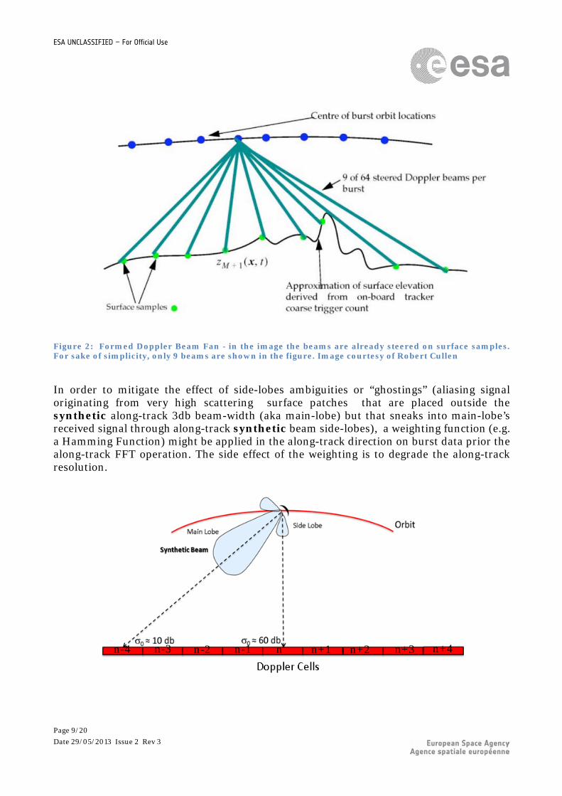
Figure 2: Formed Doppler Beam Fan - in the image the beams are already steered on surface samples. For sake of simplicity, only 9 beams are shown in the figure. Image courtesy of Robert Cullen

In order to mitigate the effect of side-lobes ambiguities or “ghostings” (aliasing signal originating from very high scattering surface patches that are placed outside the synthetic along-track 3db beam-width (aka main-lobe) but that sneaks into main-lobe’s received signal through along-track synthetic beam side-lobes), a weighting function (e.g. a Hamming Function) might be applied in the along-track direction on burst data prior the along-track FFT operation. The side effect of the weighting is to degrade the along-track resolution.

n-4 n-3 n-2 n-1 n n+1 n+2 n+3 n+4



Figure 3: Side-Lobe Ambiguity Effect: the signal originating from the Doppler Cell n at nadir (high scattering patch) sneaks into the antenna through the side lobe, and overlaps and aliases the signal originating from Doppler Cell n-4 (Doppler Cell which the synthetic beam main lobe in figure is oriented towards)

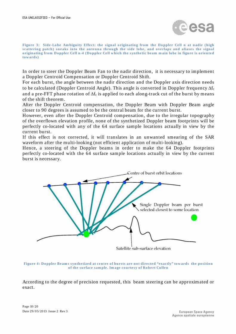
In order to steer the Doppler Beam Fan to the nadir direction, it is necessary to implement a Doppler Centroid Compensation or Doppler Centroid Shift. For each burst, the angle between the nadir direction and the Doppler axis direction needs to be calculated (Doppler Centroid Angle). This angle is converted in Doppler frequency ∆fc and a pre-FFT phase rotation of ∆fc is applied to each along-track cut of the burst by means of the shift theorem. After the Doppler Centroid compensation, the Doppler Beam with Doppler Beam angle closer to 90 degrees is assumed to be the central beam for the current burst. However, even after the Doppler Centroid compensation, due to the irregular topography of the overflown elevation profile, none of the synthetized Doppler beam footprints will be perfectly co-located with any of the 64 surface sample locations actually in view by the current burst. If this effect is not corrected, it will translates in an unwanted smearing of the SAR waveform after the multi-looking (not efficient application of multi-looking). Hence, a steering of the Doppler beams in order to make the 64 Doppler footprints perfectly co-located with the 64 surface sample locations actually in view by the current burst is necessary.

Figure 4: Doppler Beams synthetized at centre of bursts are not directed “exactly” towards the position

of the surface sample. Image courtesy of Robert Cullen

According to the degree of precision requested, this beam steering can be approximated or exact.



4.4.1 Approximated Beam Steering In the approximate beam steering, all the Doppler Beams will be steered by the same angle (here referred as Rock Angle). In order to apply the aforesaid steering, for each burst, the angle between the central beam direction and the Doppler Axis needs to be calculated (Rock Angle). This angle is converted in a Doppler frequency ∆fr and a pre-FFT phase rotation of ∆fr is applied to each along-track cut of the burst by shift theorem. By the effect of this rock steering, only the Doppler central beam footprint will be co-located “exactly”7 with own closest surface sample location whereas the other beams are steered by the same rock angle but each of them will be only approximately co-located with the own closest surface samples location. This approximation can be considered acceptable on gentle undulating surfaces.

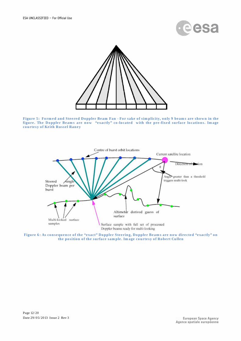
4.4.2 Exact Beam Steering For effect of the application of the Beam Formation, the Doppler Beams are angularly equispaced8 but it can happen that angularly equispaced Doppler beams produce strongly unevenly spaced projections on the ground, in event of highly variable Earth topography. In this case, the approximate steering solution does not hold anymore and it needs now to apply an “exact” beam steering. In the “exact” beam steering, each of the Doppler Beams will be steered by a different angle (Rock Angles); by effect of these phase rotations, each Doppler beam footprint (i.e. not only the central Doppler Beam) will be now co-located “exactly”9 with the own closest surface sample location. The exact beam forming needs to be applied in case of highly variable topographic surfaces.

7 Clearly, in the practical implementations, perfect exactness of the co-location can’t be achieved due to uncertainties in the knowledge of satellite's elliptical orbit, Earth ellipsoid as well as topographic relief. 8 in reality, given Earth curvature, they are only nearly equally spaced in angle over the antenna 3db along-track beam-width 9 Clearly, in the practical implementations, perfect exactness of the co-location can’t be achieved due to uncertainties in the knowledge of satellite's elliptical orbit and of the overflown topographic relief.



Figure 5: Formed and Steered Doppler Beam Fan - For sake of simplicity, only 9 beams are shown in the figure. The Doppler Beams are now “exactly” co-located with the pre-fixed surface locations. Image courtesy of Keith Russel Raney

Figure 6: As consequence of the “exact” Doppler Steering, Doppler Beams are now directed “exactly” on

the position of the surface sample. Image courtesy of Robert Cullen



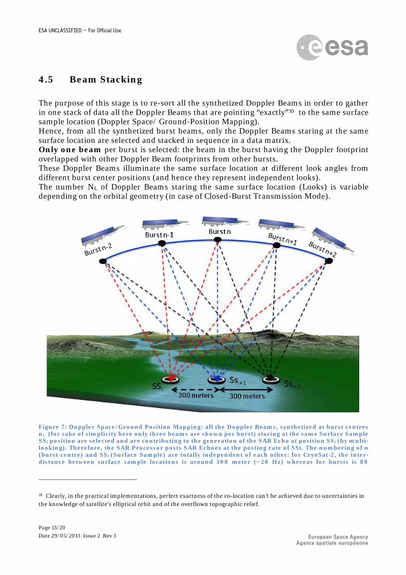
4.5 Beam Stacking The purpose of this stage is to re-sort all the synthetized Doppler Beams in order to gather in one stack of data all the Doppler Beams that are pointing “exactly”10 to the same surface sample location (Doppler Space/ Ground-Position Mapping). Hence, from all the synthetized burst beams, only the Doppler Beams staring at the same surface location are selected and stacked in sequence in a data matrix. Only one beam per burst is selected: the beam in the burst having the Doppler footprint overlapped with other Doppler Beam footprints from other bursts. These Doppler Beams illuminate the same surface location at different look angles from different burst center positions (and hence they represent independent looks). The number NL of Doppler Beams staring the same surface location (Looks) is variable depending on the orbital geometry (in case of Closed-Burst Transmission Mode).

Figure 7: Doppler Space/Ground Position Mapping: all the Doppler Beams, synthetized at burst centres n, (for sake of simplicity here only three beams are shown per burst) staring at the same Surface Sample SSi position are selected and are contributing to the generation of the SAR Echo at position SSi (by multi-looking). Therefore, the SAR Processor posts SAR Echoes at the posting rate of SSi. The numbering of n (burst centre) and SSi (Surface Sample) are totally independent of each other: for CryoSat-2, the inter-distance between surface sample locations is around 300 meter (~20 Hz) whereas for bursts is 80

10 Clearly, in the practical implementations, perfect exactness of the co-location can’t be achieved due to uncertainties in the knowledge of satellite's elliptical orbit and of the overflown topographic relief.



meters (~85 Hz). In the picture, the black and white circles represent the centres of the surface locations.

4.6 Range Alignment The purpose of this stage is to correct all the mis-alignment in range between the beams of the same stack. Indeed, if we wish to operate an efficient multi-looking, all the mis-alignment in range between the stack beams needs to be corrected. Three range corrections need to be operated and they are described in the following sub-sections:

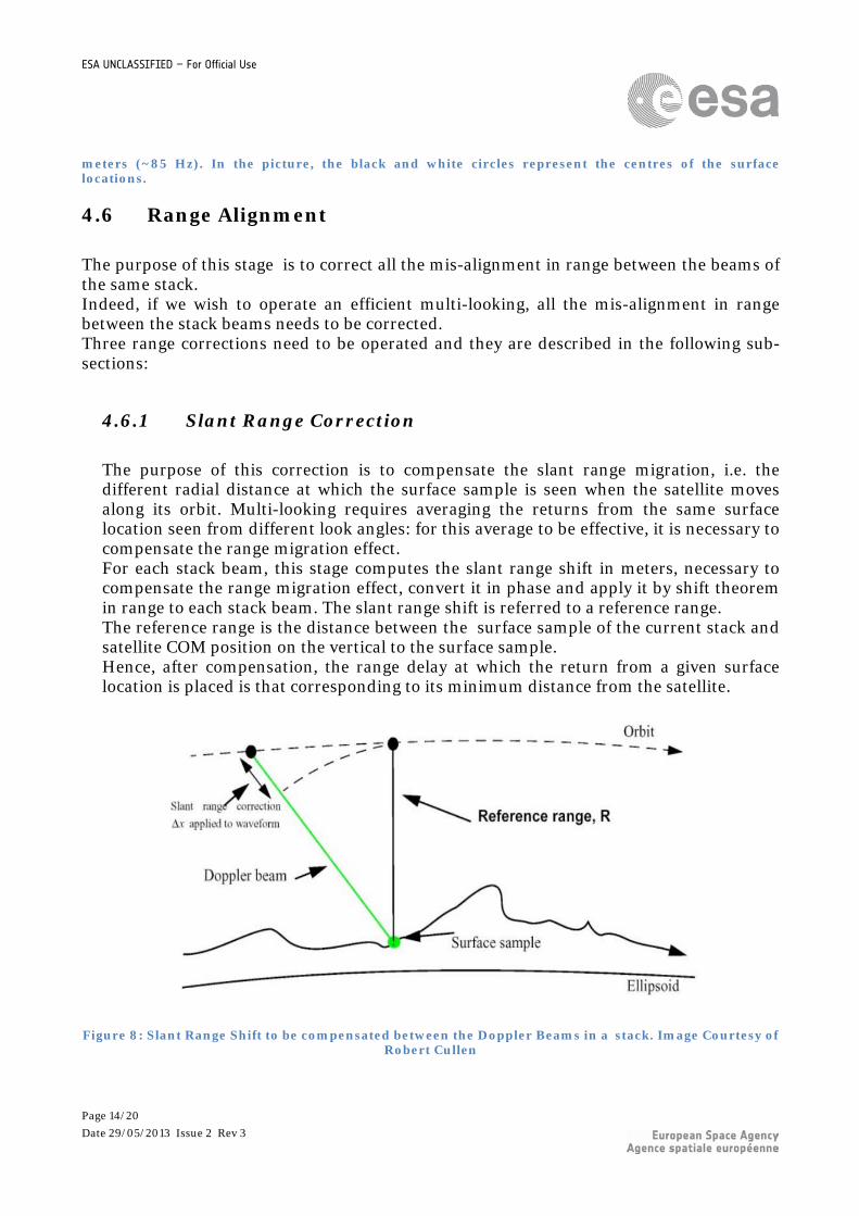
4.6.1 Slant Range Correction The purpose of this correction is to compensate the slant range migration, i.e. the different radial distance at which the surface sample is seen when the satellite moves along its orbit. Multi-looking requires averaging the returns from the same surface location seen from different look angles: for this average to be effective, it is necessary to compensate the range migration effect. For each stack beam, this stage computes the slant range shift in meters, necessary to compensate the range migration effect, convert it in phase and apply it by shift theorem in range to each stack beam. The slant range shift is referred to a reference range. The reference range is the distance between the surface sample of the current stack and satellite COM position on the vertical to the surface sample. Hence, after compensation, the range delay at which the return from a given surface location is placed is that corresponding to its minimum distance from the satellite.

Figure 8: Slant Range Shift to be compensated between the Doppler Beams in a stack. Image Courtesy of Robert Cullen



4.6.2 Tracker Range Correction

The purpose of this correction is to compensate the movement in range of the on board tracker across all the beams in the current stack. For each stack beams, this stage computes the range shift in meters, necessary to compensate the tracker movement, convert it in phase and apply it in range by shift theorem to each stack beam. After compensation, the tracker shift is that corresponding to its minimum tracker distance from the satellite.

4.6.3 Doppler Range Correction

The purpose of this correction is to compensate the Doppler shift in range for all the Doppler beams in the current stack. For each beam of the stack, knowing the angle that Doppler beam makes with the velocity vector, this stage computes the Doppler frequency shift, necessary to compensate the Doppler effect induced by sensor motion during the pulse transmission and echo reception, converts it in phase and applies it by shift theorem in range to each stack beam.

Figure 9: Formed, Steered and Range-Aligned Doppler Beam Fan - For sake of simplicity, only 9 beams are shown in the figure. The range mis-alignment between Doppler Beams is now compensated. Image courtesy of Keith Russel Raney.



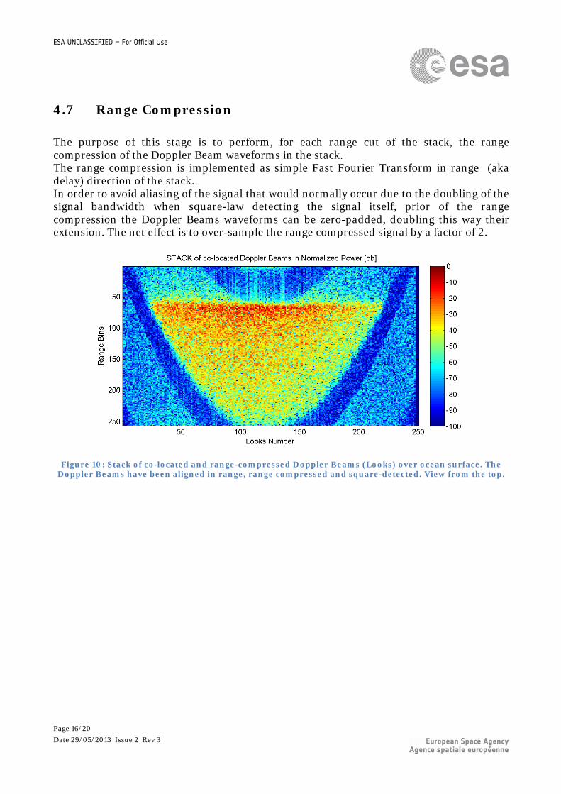
4.7 Range Compression The purpose of this stage is to perform, for each range cut of the stack, the range compression of the Doppler Beam waveforms in the stack. The range compression is implemented as simple Fast Fourier Transform in range (aka delay) direction of the stack. In order to avoid aliasing of the signal that would normally occur due to the doubling of the signal bandwidth when square-law detecting the signal itself, prior of the range compression the Doppler Beams waveforms can be zero-padded, doubling this way their extension. The net effect is to over-sample the range compressed signal by a factor of 2.

Figure 10: Stack of co-located and range-compressed Doppler Beams (Looks) over ocean surface. The Doppler Beams have been aligned in range, range compressed and square-detected. View from the top.



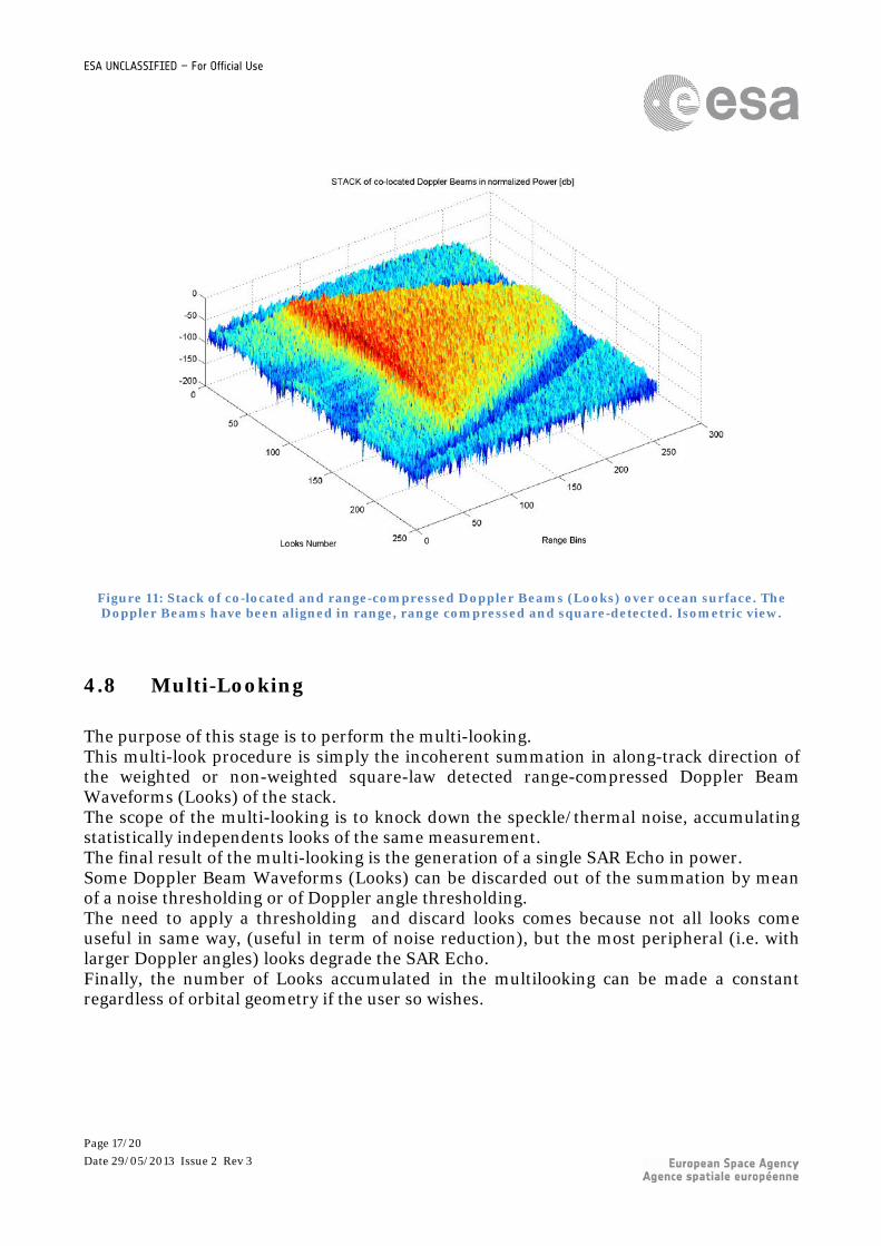
Figure 11: Stack of co-located and range-compressed Doppler Beams (Looks) over ocean surface. The Doppler Beams have been aligned in range, range compressed and square-detected. Isometric view.

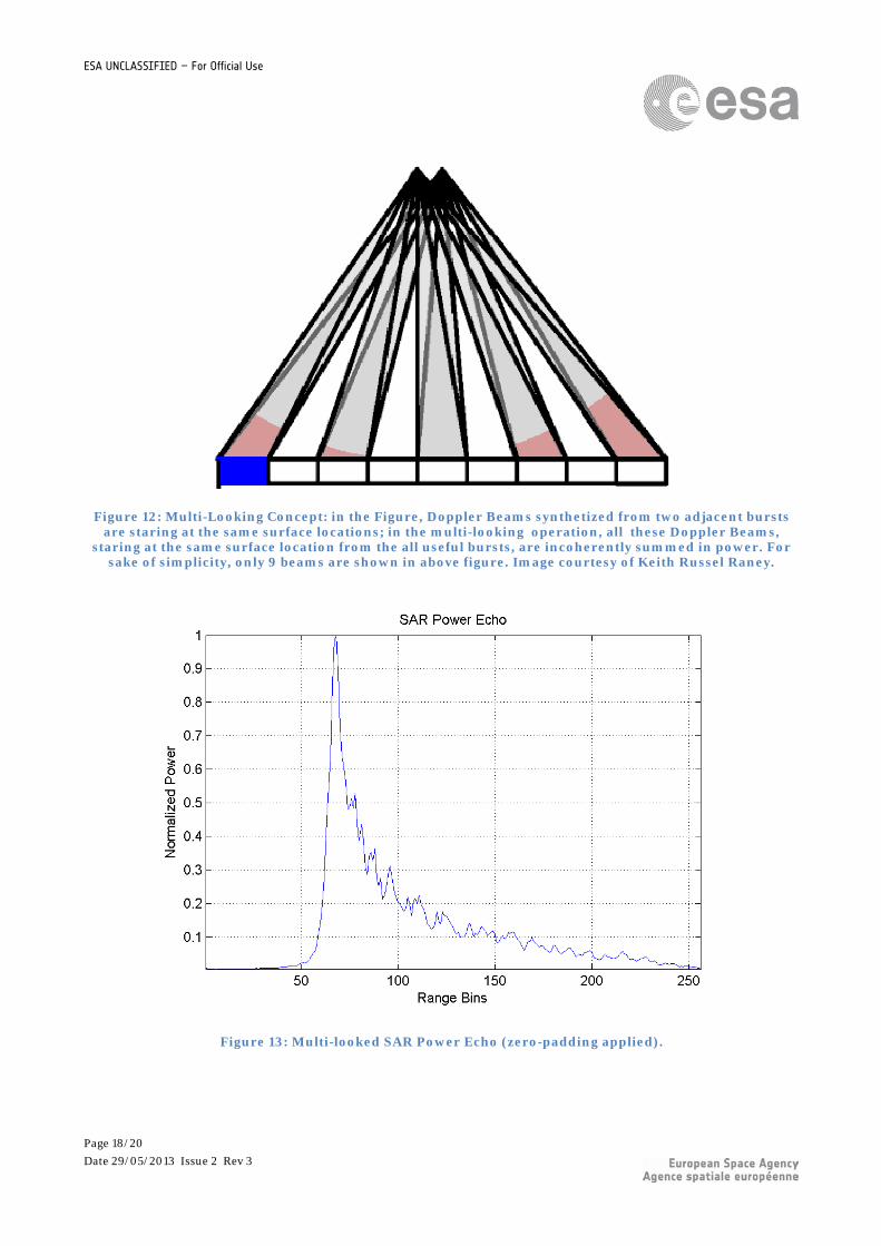
4.8 Multi-Looking The purpose of this stage is to perform the multi-looking. This multi-look procedure is simply the incoherent summation in along-track direction of the weighted or non-weighted square-law detected range-compressed Doppler Beam Waveforms (Looks) of the stack. The scope of the multi-looking is to knock down the speckle/thermal noise, accumulating statistically independents looks of the same measurement. The final result of the multi-looking is the generation of a single SAR Echo in power. Some Doppler Beam Waveforms (Looks) can be discarded out of the summation by mean of a noise thresholding or of Doppler angle thresholding. The need to apply a thresholding and discard looks comes because not all looks come useful in same way, (useful in term of noise reduction), but the most peripheral (i.e. with larger Doppler angles) looks degrade the SAR Echo. Finally, the number of Looks accumulated in the multilooking can be made a constant regardless of orbital geometry if the user so wishes.



Figure 12: Multi-Looking Concept: in the Figure, Doppler Beams synthetized from two adjacent bursts are staring at the same surface locations; in the multi-looking operation, all these Doppler Beams,

staring at the same surface location from the all useful bursts, are incoherently summed in power. For sake of simplicity, only 9 beams are shown in above figure. Image courtesy of Keith Russel Raney.

Figure 13: Multi-looked SAR Power Echo (zero-padding applied).



4.9 Delay-Doppler Processing Block-Scheme

Figure 14: Final Block-Scheme for the Delay-Doppler Processing as presented in this Technical Note.

Figure 15: Summary of the signal manipulations operated during the Delay-Doppler Processing. Please note that in the above scheme the range compression and range alignment stages are performed before the stacking stage. Image courtesy of Keith Russel Raney.

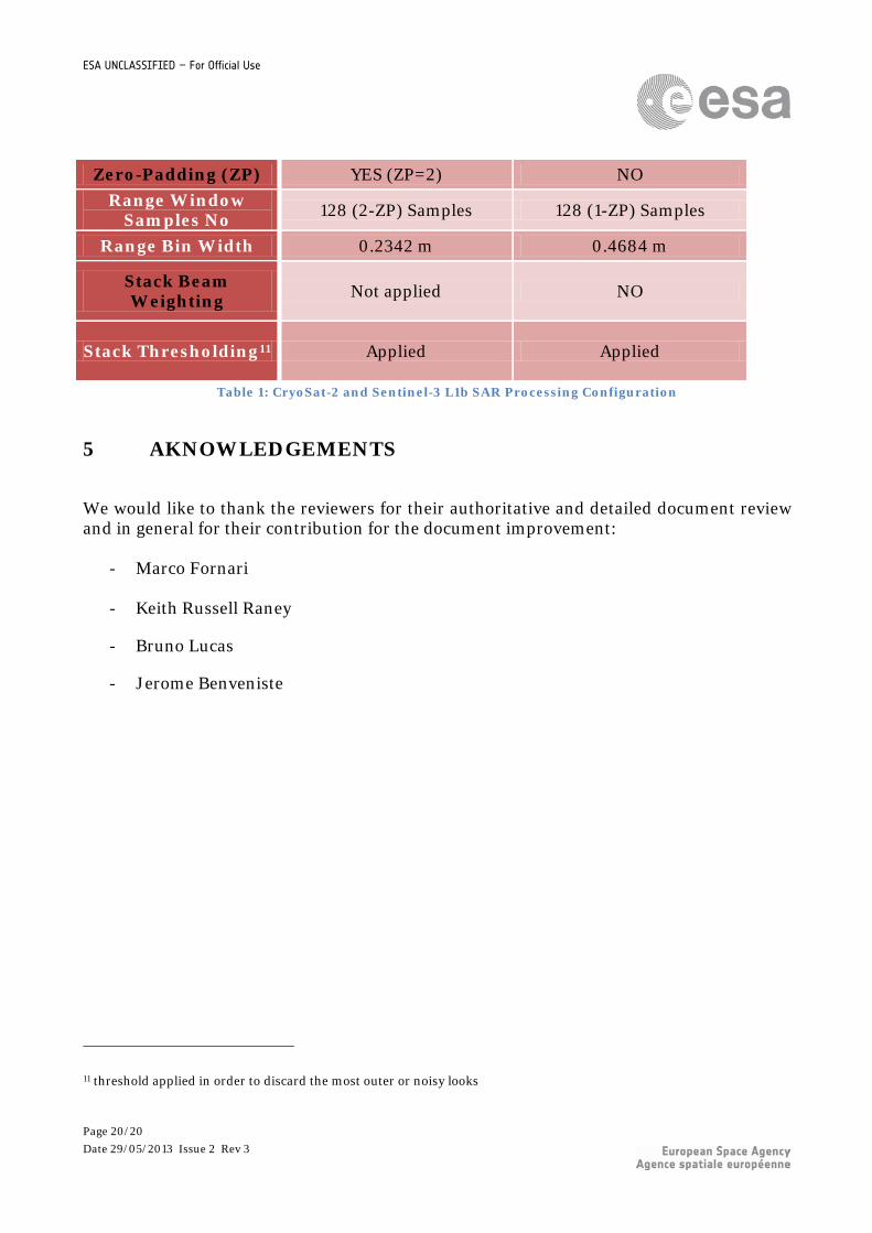
4.10 CryoSat-2 and Sentinel-3 L1b SAR Processing Configuration The following table lists the customization of the L1b SAR Processing configuration for CryoSat-2 and Sentinel-3 SAR Altimeter Ground Segment. The differences reflect the different mission’s primary objective: Ice for CryoSat-2 Processor and Ocean for Sentinel-3.

OPERATION

CRYOSAT-2 SENTINEL-3

Burst Data Weighting

YES, Hamming Window NO

Approximated/Exact Beam Forming

Both available, approximated method is

used Both available



Zero-Padding (ZP) YES (ZP=2) NO Range Window

Samples No 128 (2-ZP) Samples 128 (1-ZP) Samples

Range Bin Width 0.2342 m 0.4684 m

Stack Beam Weighting Not applied NO

Stack Thresholding11 Applied Applied

Table 1: CryoSat-2 and Sentinel-3 L1b SAR Processing Configuration

5 AKNOWLEDGEMENTS

We would like to thank the reviewers for their authoritative and detailed document review and in general for their contribution for the document improvement:

- Marco Fornari

- Keith Russell Raney

- Bruno Lucas

- Jerome Benveniste

11 threshold applied in order to discard the most outer or noisy looks


Documents

ESA Standard Document