1

ESA SPACE WEATHER STUDYALCATEL Consortium

GROUND BASED MEASUREMENTSWP 3120

November 30, 2001

Laboratoire de Physique Solaire et de l’Héliosphère, Observatoire de Paris

Laboratoire de Planétologie de Grenoble

M. Pick , C. Lathuillere and J. Lilensten

With the contribution of R. Bentley, L. R. Cander, T. Dudok de Wit, E. Flueckiger, F Jansen, P. Manoharan, B.Schmieder, P. Stauning , L. Van Driel and A. Kerdraon, JM. Malherbe, J. L. Michau, P. Picard for the pre-feasibility studies.

2

TABLE OF CONTENTS

1. Introduction ..........................................................................................................................................................................32. Scientific context..................................................................................................................................................................4

2.1 Introduction......................................................................................................................................................................42.2 Solar magnetic fields and active regions....................................................................................................................52.3 Coronal holes ...................................................................................................................................................................62.4 Coronal Mass Ejections.................................................................................................................................................62.5 Solar wind and interplanetary magnetic field ............................................................................................................82.6 Corotating Interaction Regions ....................................................................................................................................92.7 Interplantary Coronal Mass Ejections.......................................................................................................................102.8 Solar Energetic Particles..............................................................................................................................................112.9 Cosmic rays ...................................................................................................................................................................112.10 Aurora ...........................................................................................................................................................................112.11 Geomagnetic storms and substorms ........................................................................................................................12

3. Observables ........................................................................................................................................................................ 123.1 Solar magnetic field......................................................................................................................................................123.2 EUV and soft x-ray (SXR) Images..........................................................................................................................133.3 Hα + wings full disk images......................................................................................................................................133.4 Monitoring of Hard X-ray flux...................................................................................................................................133.5 Solar energy flux...........................................................................................................................................................143.6 Monitoring of radio flux at 10 cm .............................................................................................................................143.7 Radio spectra and radio imaging...............................................................................................................................143.8 Coronagraphs ................................................................................................................................................................153.9 Interplanetary scintillation..........................................................................................................................................153.10 Upstream Solar WIND and IMF.............................................................................................................................153.11 Terrestrial magnetic field variations .......................................................................................................................153.12 Cosmic rays .................................................................................................................................................................153.13 Cosmic Radio waves..................................................................................................................................................173.14 Convection electric field............................................................................................................................................183.15 Auroral precipitations................................................................................................................................................183.16 Ionospheric density ....................................................................................................................................................193.17 Thermospheric densities and temperatures ............................................................................................................19

4. Observing ground facilities: operational and under construction ...................................................................... 204.1 Full disk magnetographs and Halpha telescope networks .....................................................................................204.2 Radio Observations......................................................................................................................................................204.3 Coronagraphs ................................................................................................................................................................204.4 Measurements of interplanetary scintillation...........................................................................................................204.5 Neutron and Muon detectors ......................................................................................................................................214.6 Ground magnetometer networks ................................................................................................................................224.7 The SUPERDARN Radar............................................................................................................................................234.8 Ionosonde Networks.....................................................................................................................................................234.9 GPS receivers ................................................................................................................................................................244.10 Incoherent Scatter radar.............................................................................................................................................254.11 Optical Interferometers ..............................................................................................................................................264.12 Riometers .....................................................................................................................................................................26

5. Space-borne and ground-based segments ................................................................................................................. 275.1 Sun and Heliosphere ...................................................................................................................................................27

5.1.1 Preliminary remarks ............................................................................................................................................275.1.2 space- and ground segments ...............................................................................................................................27

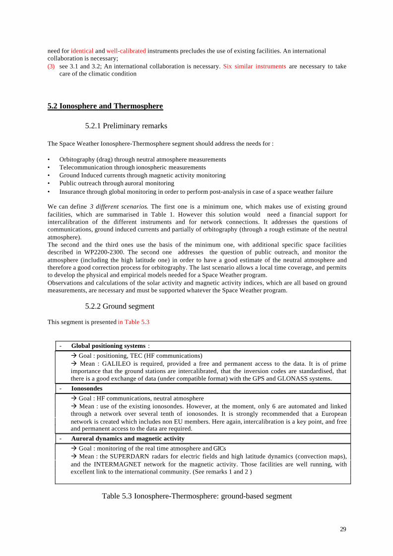
5.2 Ionosphere and Thermosphere ...................................................................................................................................295.2.1 Preliminary remarks .............................................................................................................................................295.2.2 Ground segment................................................................................................................................................... 29

6 Appendix Technical requirements for space based radiospectrograph ..............................................................316.1 Goals and constraints ...................................................................................................................................................316.2 Proposal..........................................................................................................................................................................31

7. Appendix Ground based segment:some cost estimates.......................................................................................... 33References (incomplete)...................................................................................................................................................... 35

3

1 Introduction

Space weather requires data monitoring that can be obtained from space borne and/or ground based instruments.In this report we define the parameters that are needed with emphasis on ground-based instruments. Elaborationof this report has received input from various team members, consultants and also from other team reports, inparticular from: WP 2200 and 2300 (space segment), WP 2100 (space weather parameters), WP 1300 and WP1400 (space weather parameters required by the users and synthesis of the user requirements).

We have defined in a first approach the physical phenomena and the required observations without distinctionbetween ground or space measurements. Then, when the observations can be made by both techniques , ourcriteria are the need to cover 24 hours and a high priority to space borne instruments, when suitable.Moreover, to establish our preference between space or ground, we have been led to make some preliminarypre-feasibility studies briefly presented.Table 1 summarises the conclusions of this report and presents the required Earth-based instruments necessaryto observe a given space weather inducing phenomenon. In addition, it is important to note here that theobservations and calculations of the solar activity and magnetic activity indices should also be supported by anySpace Weather program. More specifically, targets and corresponding solar and interplanetary observablesare summarised in Table 3.1 . Similar information has been provided for the ionosphere and thermosphere, inWP 1300 and in First Iteration. Table 5.1 presents the space-borne segment limited to the Sun andInterplanetary medium (see WP 2200-2300). Tables 5.2 and 5.3 present the ground-based and space-bornesegments.

4

Table 1.1 Required Earth-based instruments necessary to observe a given space weather inducingphenomenon

Instrument

C

ME

ons

et

CM

E p

ropa

gatio

n

CM

E (f

ew c

oron

alpr

oxie

s)

Flar

es

Flar

es w

ith p

roto

ns

Cor

onal

hol

es

Shoc

ks

Mag

netic

clo

uds

Ups

trea

m p

lasm

aco

nditi

ons

Geo

mag

netic

sto

rms

and

subs

torm

s

Cos

mic

Ray

Par

ticle

s

Rad

iatio

n be

lten

hanc

emen

ts

Rin

g cu

rren

t cha

nges

Iono

sphe

ric d

ensi

tych

ange

s

Scin

tilla

tions

Aur

oral

ova

l sha

pe &

dyna

mic

s

Con

vect

ion

patte

rn

Magnetograph (1) ? ? X X X ? XCoronagraph (1) ?H-α imager (1) X X X XRadio spectrograph (2) ? X X X X XRadio imaging X ? X X X X XInterplanetary scintillation X X XMagnetometer network X X X XHF radar network XIonosondes XGPS receivers X XRiometers X X XNeutron and muon monitor X X X

N.B.: The instruments marked with a (*) provide fundamental parameters which are used in space weatherforecasting or monitoring at present. The other instruments are at present used for research but may ultimately beused operationally.

(1) Our first choice is to recommend space-based instruments.(2) For frequencies below 400 MHz , we recommend a space based radiospectrograph

2. Scientific context

2.1 Introduction

Earth environment and geomagnetic activity are controled by ionized solar plasma, the solar wind which flowsoutward from the sun to form the heliosphere. The solar wind is divided between streams of slow (~300km/s)and fast solar wind (700 km/s). The steady fast wind originates from open magnetic field regions at the sun, thecoronal holes. The solar wind is affected by solar activity. The most dramatic solar events affecting the terrestrialenvironment are solar flares and Coronal Mass Ejections (CMEs). They are the primary cause of majorgeomagnetic storms and are associated with essentially all of the largest solar energetic particle events. Theradiation effects occur immediately, the particle effects occur within tens of minutes to days. Geomagneticstorms are correlated with CMEs that reach the Earth environment within 2-4 days. The origin of CMEs andflares is still questionable but there is a consensus that magnetic energy release is the source for both flares andCMEs. Flares occur in a localized region while CMEs are due to a large scale reorganization of the coronalmagnetic field produced by a loss of stability. CMEs are easily observable at the solar limb by coronagraphs overthe dark background. However Earth-directed-disk CMEs, so-called Halo events, are much more difficult todetect. Consequently, establishing the correlation between solar surface magnetic disturbances, coronalmanifestations and CMEs is a fundamental question to understand origin, initiation and development of CMEs.It is of primary importance for space weather.Solar Energetic Particle Events (SEP) which result from solar flares and CMEs can reach high energy rangingfrom tens of MeV to over a GeV. These particles can reach the Earth very promptly after the flare occurrence ormore gradually.

5

Geomagnetic storms and more generally geomagnetic activity affect the magnetosphere, the ionosphere and thethermosphere.In the magnetosphere, they have a drastic effect on the radiation belts and on the plasmasheet, which are tworegions crossed by most of the spacecrafts. Moreover, the opening of the subdiurnal magnetopause makes somespacecraft to be directly exposed to the high energetic solar wind. Finally, storms can compress themagnetopause toward the Earth below the altitude of the geostationary orbit.In the atmosphere, they result in more particle precipitation which can reach middle latitude and enhancedelectric fields. Consequences are fast variation of the electron density (effects on communication), generation ofgravity waves (effects on orbits), heating of the thermosphere (effects on orbits), ground induced currents(effects on power companies, petrol companies …). All these effects are detailed in WP 1300.

2.2 Solar magnetic fields and active regions

The solar magnetic field reveals many fine-scale structures which are not distributed at random on the solarsurface. Flux tubes, coronal holes, energetic flares and the 11 year solar cycle all depend on the configuration

Figure 1 Left panel: Hale law for the present cycle. Middle panel: Helicity law for active regions and filaments, cycle independent. Rightpanel: Helicity inside magnetic clouds (from Bothmer and Schwenn, 1994).

and dynamics on the field. Active regions are concentrated into complexes of activity associated with thedevelopment of larger regions of background magnetic field. Twisted magnetic flux that emerges into thephotosphere forms sunspots, active regions and filaments (prominences). Eruptive flares and CMEs occur inmultipolar topologies involving large and small scale regions. Eruptive events, flares and CMEs, result from anenergy release that has been stored in these regions. ( see the models in WP 2100). Magnetic shear and twist,exceeding a critical value (e.g. >70° shear angle) can lead to the destabilization of these regions. In the presentstate of our knowledge we cannot predict the exact timing of a flare or CME occurrence. Nevertheless assummarized below, magnetic field measurements are of primary importance to:- Safely forecast periods of quiet solar activity and periods of high activity,- Identify among all CMEs whose that will be the most geoeffective.- Develop numerical modeling of the solar-terrestrial system.

Conditions for the generation of flares and CMEs

? About 93% of flares arise in active regions which contain sunspots. Proton flares occur in active regionshaving two sunspot rows of opposite polarity. Magnetic evolution like flux emergence or shearing motions willlead to the flare occurrence.

? A significant portion of CMEs contain an erupting filament which presents a high level of helicity, but theinstability levels are presently not known. Destabilization of the structure is due to the magnetic evolutionobserved in the form of:

- Small-scale flux emergence or flux cancellation along the magnetic inversion line, i.e. under thefilament.

- Larger-scale flux emergence or, in general, magnetic field evolution in the vicinity of the filament.

6

? Large-scale CME events are often produced in association with a flare. Multipolar topology of these eventsinvolve large transequatorial loops connecting two active regions. Having the same sign of helicity increases theprobability of inter-AR connectivities and such connectivities can be destabilized by eruptive events at eitherfootpoint. In addition, if an active region disobeys the hemisphere helicity rule (i.e. negative on the northern andpositive on the southern hemisphere) not only increases the probability of CMEs involving both hemispheres,but also, possibly, represents an increased CME-probability (Figure 1).

2.3 Coronal holes

Coronal holes correspond to open magnetic field regions at the sun and are the source of high-speed solar windstreams. Because of their lower density, they are observed as brightness depressions on X-ray images and radiomaps from centimeter to meter wavelengths. Coronal holes can remain stable for many months

2.4 Coronal Mass Ejections

The observations suggest two classes of CMEs:-Slow CMEs associated with prominence/filament eruptions; many of them accelerate when they move outthrough the corona and may reach similar speeds as the CME/flare events.-Fast CMEs are most often associated with flares. They show no evidence of acceleration and appear to movewith nearly constant speed, may decelerate in the interplanetary medium. These flare/CME events are most oftenassociated with large energetic particle events and the particles reach the Earth environment within tens ofminutes.There is no clear-cut distinction but some overlap between these two classes. Large majorities of CMEs, whichare associated with large geomagnetic disturbances, correspond to Halo-CMEs. Surface and coronalmanifestations correlated with CMEs can be used as proxies .

CME's associated with erupting filament/ prominences

A large majority of slow CMEs in the corona are associated with eruptive prominences. Seen on the limb, theyhave been described as a three-part structure consisting of a bright loop overlying a coronal cavity containingbright core of denser material coming from an eruptive prominence. Disk events correspond to eruptivefilaments for which Doppler shift (>60 kms -1) are observed (Schmieder et al., 2000), sometimes several hoursbefore the filament erupts. Large magnetic shear is detected along the inversion line. It is plausible to assumethat the orientation of the CME's is closely associated with the orientation and location of the underlyingfilament.

Flare-CME events

Most of the flare CME events result from an initial perturbation leading to a further destabilization on a muchlarger magnetic multipolar arch system; the resulting CME will cover a large latitudinal and longitudinal range.The underlying magnetic geometry of CME’s can involve connections between the flare region and widespreadmagnetic regions sometimes on the opposite sites of the equator. These large loop systems are seen in radio, Xrays and/or in EUV before the CME occurrence. These loops are rising up in the corona and the expansion ofthe plasma leads to a dimming. These dimming regions are identified by their strong depletion in coronal EUVemission within half an hour of the estimated time of CME lift-off. Large loop systems and the dimming areasprobably map out the "footprint" of the CME’s (Thompson et al., 2000; C Delannée, 2000 ).

Radio imaging observations have shown that CMEs spread from an initial small volume in the corona in thevicinity of the flare site and are built up by successive interactions with coronal structures at progressively biggerdistances from the flare site. Signatures of these interactions are non-thermal emissions in the metric wavelengthrange. CMEs reach their full angular extent in the low corona in time scales of several minutes (Maia et al.,1999; Pick et al., 1999.).Following step by step the CME development for this category of flare/CME events, early magnetic interactionis followed by subsequent magnetic interaction at the flare site which represents the main phase of energyrelease, leading to particle acceleration and the production of a blast wave called Moreton wave when detectedin Hα. The observations suggest that this wave originating from the flaring region and propagating in the coronamight lead to further destabilization and magnetic interactions when it encounters other large or small scalecoronal structures. These interactions are detected in radio and results in the generation of fast plasmoids and ofsecondary shock waves leading to coronal radio type II bursts. Recent results suggest that the total extent of a

7

CME is correlated with its velocity (Maia, 2001). CME-driven shocks are also associated with the leading edgeof these fast ejecta moving up in the corona.

Tracking a CME-driven shock prior to its in-situ detection at the Lagrange point

Type II radio bursts are attributed to plasma waves excited by shocks and converted into radio waves at the localplasma frequency and/or its harmonics. On spectrograph data, the type II emission is observed to drift towardlower frequencies. This frequency drift results from the decrease of the plasma density as the shock propagatesfurther from the Sun. They are usually observed below 400 MHz. Kilometric type II radio emission from 30kHz to a few MHz are produced in the interplanetary medium.

Figure 2. Dynamic spectrum of the Wind/WAVES radio data for the period of May 12-15, 1997 in the frequency range from 27 kHz to13.825 MHz. The ordinate scale is the inverse of the observing frequency. The dynamic spectrum was purposely over exposed to bring outthe very weak type II radio emissions. The observed weak type II radio emissions for this event lie along straight lines, labeled F and H, thatoriginate from the CME solar lift-off time of ~05:10 UT on May 12. These radio emissions are generated up stream of the CME-drivenshock at the fundamental and harmonic of the plasma frequency (from Reiner et al., 1998).

What has been firmly established is the association between interplanetary type II bursts and CME-driven shocks(Cane, Sheeley and Howard, 1987). Interplanetary radio emission is generated upstream of the CME-drivenshock (Reiner and Kaiser,1999). Figure 2 displays an example of interplanetary type II bursts: the radio intensityin the dynamic spectrum has been plotted versus 1/f where f is the frequency. As the interplanetary density variesas R-2, R being the radial distance from the sun, the plasma frequency fp must vary as R-1 and thus 1/f versustime will vary as R. Assuming a shock is travelling with a constant velocity v, type II radio emissions will beexpected to be organized as a straight line since R=v(t-t0), t0 being the lift-off time. The type II emissionsdisplayed in Figure 2 lie along two straight lines labeled F and H. The straight line corresponding to F emissiongoes from the solar lift-off time to the measured plasma frequency upstream of the shock. As well as for shockwave originated type II emissions, dynamic radio spectra of type III bursts (see also in Figure 2) also allows thedetermination of the propagation velocity of energetic electron beams (in the order of 100000 km/s) andconsequently the estimation of the arrival time at near Earth orbit for shock waves and electrons (Mann et al.,1999).These examples clearly illustrate the importance of tracking the radio disturbances in the interplanetary mediumand particularly when the radio instrument is equipped with antennas having the direction finding capability. Thesame example, however, shows also the limitation of this method. Indeed, interplanetary type II emissions arecomposed of discrete, narrow frequency bandwidth features , dispersed in time and thus the type II identificationmay be rather delicate to establish before having obtained the full history of the event i.e. before the disturbancehas reached the Lagrange point. Methods for automatic detection and identification are currently beingdeveloped ( Hoang, private communication).

8

Recent results based on the combination of radio and coronagraphic images show that weak bursts drifting infrequency as type II bursts, most often not detected in spectrograph data are associated with the leading edge ofthe CMEs (Maia et al., 2000). This result shows that early phase of shock development (so called interplanetaryshock) can be detected in the corona.

Figure 3 20 April 1998 event.Composite image of one Hα image from Meudon Observatory, one NRH imageat 164 MHz (red) and one Coronagraph LASCO/SOHO image. This example illustrates the detection of type IIradio emission associated with the CME leading edge (from Maia et al., 2000).

2.5 Solar Wind and interplanetary magnetic field

The solar wind is the consequence of the supersonic expansion of the hot solar corona. It consists largely ofionized hydrogen plus a small quantity of helium and fewer ions of heavier elements. Embedded in this plasmaflow is a weak magnetic field (IMF). Magnetic field lines are frozen into the expanding plasma and because ofthe solar rotation take the shape of a spiral. The heliospheric longitude of the foot point of the spiral crossing theearth orbit is about 60° for a solar wind of 400 km/s. Two different kinds of coronal regions and wind exist: thesteady fast wind emanates from the solar magnetically open coronal holes, predominantly the polar holes,whereas the much more variable slow solar wind originates from the equatorial closed magnetic field regions,the streamer belt.

The IMF polarity is highly correlated with the photospheric field and modelling is quite successful in predictingthe polarity of IMF at 1 AU. Regions of toward and away polarity at the sun are separated by a neutral line thatextends into the interplanetary medium as a warped heliospheric current sheet (Figure 4).

The two most solar wind disturbances that affect the Earth environment are CMEs and CIR’s.

9

Figure 4 A schematic representation of the solar wind source function in the declining and minimum phase of thesolar activity function (from Balogh et al., 1999).

2.6 Corotating Interaction Regions

The increasing interaction between fast and slow solar wind streams with distance from the sun leads to thedevelopment of the Corotating Interacting Regions, CIRs. Being regions of high pressure, CIRs are bounded byforward and reverse waves that develop into shock pairs, most often beyond 1AU. Within a CIR, the streaminterface marks the boundary between the fast and slow solar wind regimes. CIRs that sweep the Earthenvironment are the cause of recurrent geomagnetic storms. They also modulates the intensity of cosmic rays

10

Figure 5 Schematic showing the expected IMF-CIR shock geometry when the ambient field consists of Parkerspiral ( from Crooker et al., 1999).

2.7 Interplantary Coronal Mass Ejections

The magnetic clouds MC are characterized by a smooth magnetic field rotation, representative of large magneticflux ropes, which is preceded by a shock. The B strength is higher than the average and the temperature is lowerthan the average. The term ejecta is given to the events for which the field rotation is not observed. Thesedisturbances are interplanetary manifestations of CMEs. It is however not yet firmly established which coronalmass ejections will be seen in the interplanetary medium as MC or ejecta.

Tracking an ICME prior to its their in-situ detection at the Lagrange point

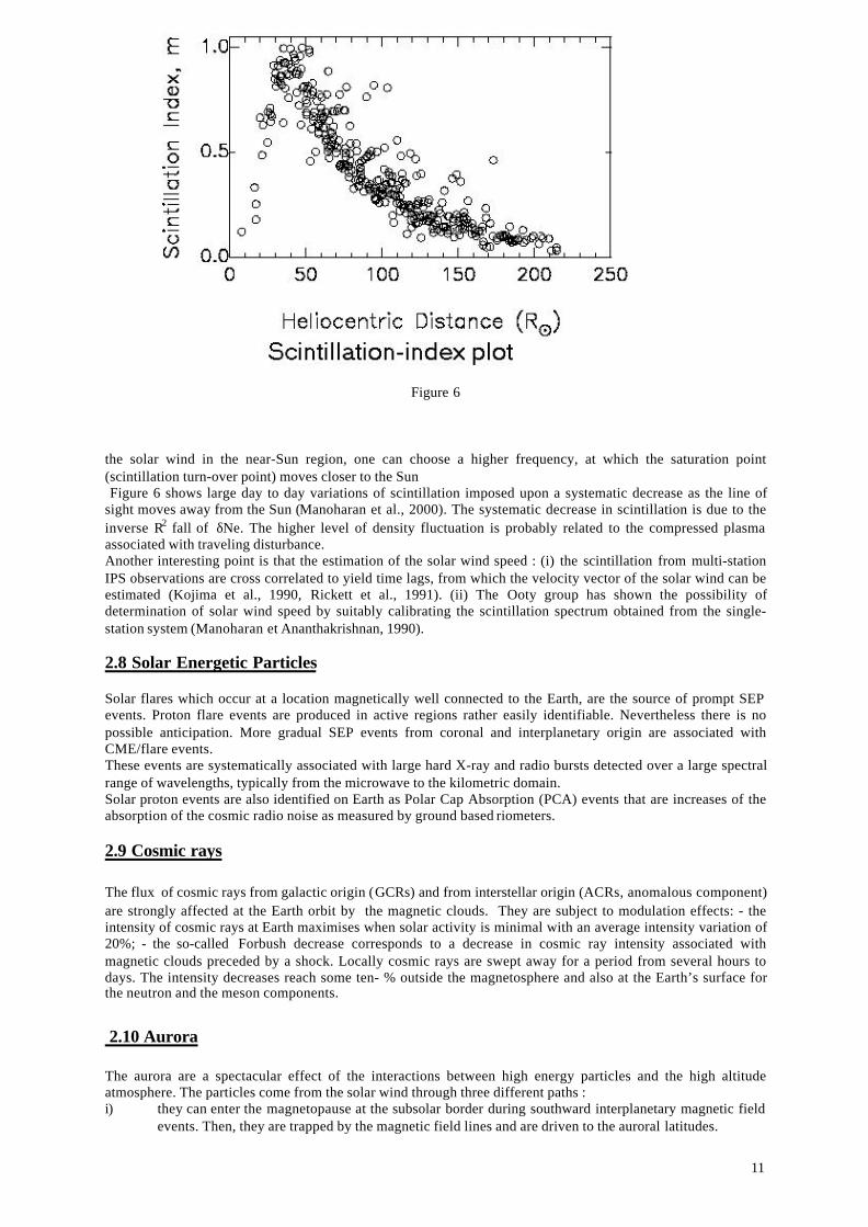
Interplanetary scintillation arises when the radiation from a distant compact radio source is scattered by electron-density irregularities in the solar wind, producing a random diffraction pattern on the ground. The resultantdiffraction pattern drifts past the observer with the velocity of the solar wind, causing temporal variation in thesource intensity. An increase in scintillation is observed when the line of sight passes through an ICME.The scintillation of a given radio sources is quantified using a scintillation index, m, which is the ratio of the rmsof intensity fluctuations to the mean intensity of the source. Since the line-of-sight distance of a radio sourcechanges due to the orbital motion of the Earth, the IPS measurements of a given source over many days providethe level of scintillation at various distances as well as at different position angles around the Sun. When thescattering is weak the measured scintillation is linearly related to the density fluctuations δNe in the solar wind.At 327 MHz frequency, the weak-scattering occurs at distances greater than about 40 Rs and however, to probe

11

Figure 6

the solar wind in the near-Sun region, one can choose a higher frequency, at which the saturation point(scintillation turn-over point) moves closer to the Sun Figure 6 shows large day to day variations of scintillation imposed upon a systematic decrease as the line ofsight moves away from the Sun (Manoharan et al., 2000). The systematic decrease in scintillation is due to theinverse R2 fall of δNe. The higher level of density fluctuation is probably related to the compressed plasmaassociated with traveling disturbance.Another interesting point is that the estimation of the solar wind speed : (i) the scintillation from multi-stationIPS observations are cross correlated to yield time lags, from which the velocity vector of the solar wind can beestimated (Kojima et al., 1990, Rickett et al., 1991). (ii) The Ooty group has shown the possibility ofdetermination of solar wind speed by suitably calibrating the scintillation spectrum obtained from the single-station system (Manoharan et Ananthakrishnan, 1990).

2.8 Solar Energetic Particles

Solar flares which occur at a location magnetically well connected to the Earth, are the source of prompt SEPevents. Proton flare events are produced in active regions rather easily identifiable. Nevertheless there is nopossible anticipation. More gradual SEP events from coronal and interplanetary origin are associated withCME/flare events.These events are systematically associated with large hard X-ray and radio bursts detected over a large spectralrange of wavelengths, typically from the microwave to the kilometric domain.Solar proton events are also identified on Earth as Polar Cap Absorption (PCA) events that are increases of theabsorption of the cosmic radio noise as measured by ground based riometers.

2.9 Cosmic rays

The flux of cosmic rays from galactic origin (GCRs) and from interstellar origin (ACRs, anomalous component)are strongly affected at the Earth orbit by the magnetic clouds. They are subject to modulation effects: - theintensity of cosmic rays at Earth maximises when solar activity is minimal with an average intensity variation of20%; - the so-called Forbush decrease corresponds to a decrease in cosmic ray intensity associated withmagnetic clouds preceded by a shock. Locally cosmic rays are swept away for a period from several hours todays. The intensity decreases reach some ten- % outside the magnetosphere and also at the Earth’s surface forthe neutron and the meson components.

2.10 Aurora

The aurora are a spectacular effect of the interactions between high energy particles and the high altitudeatmosphere. The particles come from the solar wind through three different paths :i) they can enter the magnetopause at the subsolar border during southward interplanetary magnetic field

events. Then, they are trapped by the magnetic field lines and are driven to the auroral latitudes.

12

ii) they can cross the magnetopause on its sides principally on the night side of the Earth. They feed theplasmasheet and under the coordinated effect of the geomagnetic field and the interplanetary electricfield, are driven back toward the Earth, until they are also trapped by the magnetic field lines and aredriven to the auroral latitudes.

iii) they may be trapped directly by the geomagnetic field above the cusp : there, the field lines are openonto the magnetosheat.

The two first class of particle experience an acceleration in the bow shock, which enhance their energy up toseveral hundreds of keV. The last class of particles are not accelerated and therefore enter the atmosphere withsmall energies.When these particle collide the atmosphere, they can ionize, excite, dissociate the atoms or molecules.Dissociated atoms and ions may be in excited states. The way back to ground state can occur through chemicalreactions, or through the emission of electromagnetic beams, some of them being in the visible spectrum. This isthe origin of the aurora.

2.11 Geomagnetic storms and substorms

Depending on fast or slow solar wind regims, the interplanetary magnetic field may experience multiplereversals. Recombinations may occur between the subsolar magnetopause and the interplanetary magnetic field(this phenomenon is known as a “transfer flux event”, and partly explained by the theory of the “openmagnetosphere”, (Stern 1996, and references herein). The solar wind can enter directly the magnetosphere on theday side. The magnetopause is pushed toward the Earth, sometimes below the geostationary spacecraft orbit (6.6Earth radii). The literature is not very precise on the definition of geomagnetic storms and geomagneticsubstorms. We can make a rough distinction : substorms are the effects of the transfer flux events when only thehigh latitudes are affected. Geomagnetic storms correspond to planetary effects of the transfer flux events. Whenit is the case, more solar wind particle cross the magnetopause (growing phase of the storm), and therefore, theplasmasheet becomes much thicker. The particle precipitation are enhanced, the auroral oval takes a θ shape(expansion phase) and the electric fields increase to several tenth of mV/m. The outer border of the plamapausegoes down to 2 to 3 Earth radii. The polar wind populates the plasmasheet with oxygen ions up to 40% between10 and 23 Earth radii.The enhanced precipitation create brighter aurora, and more electron production in the ionosphere, sometimes atmiddle latitudes. It also creates a strong heating rate. Since they depend on the temperature, the chemicalcoefficients are modified, which turns in depletions of the electron density. The effect of the precipitation on theionosphere is instantaneous. Therefore, during the storms, strong and fast local variations of the electron densityoccur.There are also several effects on the thermosphere. A thermospheric heating occur through collisions withprecipitation, and through Joule heating due to the electric field. This results in an expansion of thethermosphere. Finally, the energy which is deposited at high latitude expands toward the equator through gravitywaves.

3. Observables

3.1 Solar magnetic field

Full disk magnetograms provide the large and small scale topology of the magnetic field. This is necessary for:

Prediction of:CME and flaresShape of the heliosheetGeoeffective CIRs and ICMEs (sign of Bz)

No significant geomagnetic activity is seen unless the interplanetary magnetic field has a southward component(Bz negative at the sun), antiparallel to the earth 's magnetic field near the subsolar point at the daysidemagnetopause. A southward interplanetary field interconnects with the earth’s magnetic field.

13

CMEs that will develop into geoeffective ICMEs are those having a substantial negative transverse magneticfield Bz. The sign of Bz can be derived from the sign of helicity and from the Hale law (see Figure 1) for manyCMEs. However this is more difficult to be predicted in the case of large-scale CME eventsThe geoeffectiness will also depends on the respective location of the Earth and of the plasma sheet extrapolatedfrom the photospheric field.

These measurements can be obtained from space or from ground. Magnetograms with a spatial resolution of 2arcsec/pixel and temporal resolution of the order of 15 minutes are needed. We propose a space based instrument(see WP 2200 and 2300). Moreover, vector ground based magnetographs will be used to show changes onshorter time scales and also for the helicity computations.

3.2 EUV and soft x-ray (SXR) Images

Coronal holes are well observed in EUV. Their observations are needed for:

CME predictionSigmoid precursor structures (twisted magnetic field) are present in over 50% of CMEs (Sterling, 2000;Van Driel et al., 2000). These sigmoid structures are more apparent in SXR images than in EUVimages, indicating that they are hotter features than those typically seen in EUV

Diagnostic on the large scale topologie

CMEs detectionCMEs are associated with long-duration SXR events called LDEs. The correlation can reach 100 %for events of duration > 6 hours. (Sheeley et al., 1983), typically 1-8 Å.

Imaging observations coordinated with Hα and radio imaging observations determine the foot print(dimming) of the CME thus the extend in latitude and longitude and the orientation.

3.3 Hα + wings full disk images

These observations are needed for:

Monitoring of solar activity

Flare and CME predictionExcellent tracers of filaments and active centers; they are a complementary tool to magnetic field andXUV measurements to determine the large scale topologie

Provide the dynamical behavior of filaments and prominences

Flare and CME onsetsFlare location

Observation of Erupting filaments

Detection of Moreton waves

These observations can be obtained from space or ground and we propose for the first time a space-based Hαtelescope. Pre-feasibility study is presented in WP 2200 and 2300.

3.4 Monitoring of Hard X-ray flux

Diagnostic on SEP events

14

3.5 Solar energy flux

The extreme ultraviolet (EUV) solar flux is energetic enough to ionise the upper atmosphere. It constitutes themajor source for the diurnal ionosphere. Most of the current models rely on few experiments taken onboard theDynamics Explorer missions (Hinteregger,1973, Hinteregger et al. 1981, Tobiska , 1991; Tobiska and Eparvier,1998, Richards et al., 1994).Those models are very important for aeronomic computation. However, they cannot take into account thevariability at different wavelengths. It is therefore not surprising that several instruments will be soon launchedin order to solve the problem of the determination of the solar flux in this domain (UV, EUV, XUV). The SEEinstrument onboard the TIMED spacecraft (www.timed.jhuapl.edu/home.htm will be devoted to it.A radically different approach has been undertaken by Warren and co-authors (Warren et al., 1998). Theycombined different data and models to synthesize the irradiance from EUV line emission formed in the upperchromosphere and lower transition region from the Ca II K-line through the model. This approach rises a newquestion, which is the variability of the EUV spectrum versus specific solar zones (quiet sun, coronal hole …)and, in a single zone, versus time.Finally, the TIGER Program was established within the framework of the SCOSTEP International Solar CycleStudy. This decision is based on the general agreement that the improvement of existing thermospheric-ionospheric (T/I) models is absolutely necessary to meet scientific and engineering goals for thermospheric-ionospheric research as well as for a broad range of commercial applications in space. There are also a numberof scientific questions underlying the goal of understanding solar EUV/UV variability such as what are theprimary mechanisms by which solar ultraviolet (UV), extreme ultraviolet (EUV), and soft X-ray (XUV)irradiance variations affect terrestrial global climate change with the upper atmosphere included and spaceweather.

In summary, the improvement of T/I models in the frame of space weather requires coordinated work onmeasurement and modeling of solar EUV/UV radiation and on EUV/UV Space Instrumentation, since theseobservations can only be made from space.

F10.7 cm as proxy of the solar EUV flux

The Earth atmosphere is transparent to solar radiowaves around a few centimeters. Since 1947, the 10.7 cmwavelength has been chosen as proxy for the solar EUV flux. Its intensity is called the decimetric index f10.7 . Itis expressed in 1022 W.m-2.Hz-1. It ranges from about 70 for quiet solar conditions to about 350 for active sun.This index is today used in most operational and physical models of the ionosphere and thermosphere (Table 2of WP2100). It is very important for the continuity of the geophysical records that this index continues to bemeasured permanently.

3.6 Monitoring of radio flux at 10 cm

In addition to the interest of measuring the flux at 10cm as proxy of the solar EUV flux and solar activity, Bala etal. have recently investigated 40 years of solar radio burst data in the frequency range 1-20 GHz (Bala et al,2001). They discussed the rate of occurrence of events (>103 SFU) in the context of the noise levels in typicalwireless communication systems. They found that a wireless cell site could suffer severe interference from asloar radio burst on several occasions in a year, especially during solar maxima.

3.7 Radio spectra and radio imaging

These observations are needed for:Location of the neutral sheet provided by the imaging observations of the quiet sun at decimetric wavelengths.

Signatures of B field emergence and interaction

Signatures of SEP events, and energetic electron beams over a large range of altitude

Shock signatures over a large range of altitude

CME initiation and development

Spatio-temporal history of flare-CME events in the corona

15

Imaging observations coordinated with Hα and radio imaging observations determine the foot print(dimming) of the CME thus the extend in latitude and longitude and the orientation.

Projected velocities above the solar disk

We propose to monitor:

Spectral observations covering the 20 GHz-30 KHz spectral domain. Because of the ionospheric effects, radioemissions at frequencies below 10 MHz cannot be performed from the Earth.

Imaging observations covering a frequency range of approximatively 700-70 MHz.

3.8 Coronagraphs

CME development over a large range of altitudes

3.9 Interplanetary scintillation

ICME propagation in the interplanetary medium prior to in-situ detection

Although, the IPS method represents a measurement, which is line of sight integrated, it has several advantages.It is one of the few remote sensing techniques by which one can observe the dynamics and structure of the solarwind in three dimensions, including regions where in situ measurements are not easily possible, e.g., near theSun or at high helio latitudes. This inexpensive method is being used for the long-term monitoring of the solarwind over a large period of time, i.e., over solar cycles. In the study of energetic transients which leaves the outercorona, there is a large observational gap between the while-light coronagraph measurements and about 1 AUwhere interplanetary shocks are recorded by spacecraft. Since there may be considerable evolution of physicalproperties of transients on their way from Sun to Earth, the lack of information in the Sun-Earth distance is oneof the major drawbacks in the understanding of transients in the line, which transients are geoeffective and whichones are not. IPS method provides unique information on the location and nature of propagation of large-scaletransients. IPS-imaging and requires daily scintillation measurement on a grid of radio sources over the wholesky.

3.10 Upstream Solar WIND and IMF

Most SW prediction services are entirely based on use of upstream conditions: Solar wind density and velocityand IMF topology. Today, these data are gathered at the L1 Lagrange point by the ACE and WIND spacecraft.In situ monitoring of these quantities is required since they are key parameters to forecast the geomagneticstorms and substorms.

3.11 Terrestrial magnetic field variations

Magnetic field variations are used to derive the different planetary magnetic indices (see WP2100 and its annexD) which are today inputs of most Space Weather operational models as indicated in Table 3 of WP2100, andalso of physical model of the magnetosphere, ionosphere and thermosphere (Table 2 of WP2100).

Furthermore, at high latitude, observations of the variations of the geomagnetic field provide a direct signature ofthe ionospheric currents that affect some space weather users : power generation and supply, oil and gas pipelinegeneration, railways, as identified in table 11.2 of WP-1300. These observations are useful to identify the Solarwind pressure pulses and the magnetic storms and substorms as outlined in Table 11.1 of WP-1300, and can beused to derive the convection electric field as described in WP-2100 (p24-25), when combined to others ground–based and spatial measurements.

3. 12 Cosmic rays

16

Approach of CMEs is detected through specific signatures in the intensity-time profiles of cosmic rays. Thesesignatures are the result of the interaction of cosmic rays with interplanetary CME driven shocks. Theycorrespond either to an intensity deficit confined in a small pitch angle region around the sunward IMFdirection (loss cone effect due to the cosmic-ray depleted region behind the shock) or to an increase or decreasewhich does not systematically align with the IMF direction. Such observations are done with ground-levelmultidirectional muon detectors. Recently muon monitoring was proposed to be a tool to forecast geomagneticstorms several hours in advance (K. Manukata et al, 2000).

Among the Space Weather users, the civil aviation has to assess radiation doses due to Galactic cosmic rays andSEP events, to aircrew as the result of a new European legislation (see WP1300-1400). The SIEVERT project ofDGAC (Direction Générale de l’Aviation Civile in France) aims to calculate these doses using neutron monitordata and models of particle transport. It should be operational in June 2001, using observations made by theKerguelen and Terre-Adelie neutron monitors operated by IFRTP (Institut Français de Recherche et deTechnologie Polaires) and cosmic ray previsions provided by Observatoire de Paris 18 months ahead. SIEVERTis today based on a program developed by the US Federal Aviation authority, that calculates the dose as afunction of the altitude, the geographical coordinates and the heliocentric potential deduced from neutronmonitor observations. This program should be replaced in the future by a new one developed under a EuropeanUnion contract.

17

Table 3.1 summarizes the most significant solar and interplanetary targets to be reached, the observables and thecorresponding key parameters.

Forecast Targets Observables Key parameters Space (S)or

Ground(G)

Coronal Holes, originof fast solar wind

Xray and EUV imaging Brightness depletion S

Neutral sheet,prediction of helio. CS

Solar magnetic fieldsRadio imagingCoronagraphs

Field measurementsThermal emission topologyStreamer belt

S, GGG, S

Steady IPmedium

CIRs In-situ measurements See WP 2200 and 2300 SCME and flareprediction

Solar magnetic fieldsHα imagingX ray and EUV imaging

Polarity, shear, helicityHα velocities, topology Sigmoids, topology

S, GS, GS

CME onset anddevelopment in corona

X ray and EUV imagingHα imagingRadio spectra (GHz-MHz)Radio imaging (750-75 MHz)

Coronagraph

Structural changes, dimmingHα velocities, Moreton wavesShocksSpatio temporal evolutionorientaton and extendProjected velocities

SS, GS , GG

S,G

ICMEs

Forecast at 1AU

Radio IP scintillationRadio spectraWhite light imagersIn-situ measurementsMuon detectors

ICME propagationIP shocksICME propagationParameters (WP2200 and 2300)Intensity of cosmic rays

GSSSG

ICME at1AU

Prediction ofgeoeffective CMEs

Solar magnetic fields Sign of Bz S, G

SEP Solar energetic events,Link with SEPSEP

Hard X-rays flux and imagingRadio spectra and imagingIn-situ measurements

Importance and location ofaccelerating sites,shockssee WP 2200 and 2300

G, partlyspace

Geomagne.Activity

Forcast from in-situmeasurement

In-situ measurements Upstream solar wind and IMF S

Table 3.1

3. 13 Cosmic Radio waves

The absorption of cosmic radio waves in the upper atmosphere is related to disturbance processes likeprecipitation of energetic particles into the upper atmosphere and heating of the ionospheric electrons by largeelectric fields. Riometers observations allow therefore to detect such events related to the solar wind-magnetosphere coupling processes like substorms as shown on Figure 7

18

Figure 7: The arrow points the onset of a magnetic substorm.

As for the use of riometers for Space Weather, one should note that a riometer provides an integrated measure ofhigh-energy particle radiation effects in the upper atmosphere. Space Weather uses are of three types:1. A polar cap riometer measures the Polar Cap Absorption (PCA) related to the solar proton fluxes followingsolar flares. This is complementary to the possible observations of the protons by interplanetary or outermagnetospheric satellites.2. A meridional chain of riometers from sub-auroral to trans-auroral latitudes will observe the border of PCAevents which gives a measure of magnetospheric compression in the solar wind (often strong compression in theenhanced solar wind following solar activity). This can be made in coarse spatial, but high temporal resolution incontrast to the sparse boundary crossings with high spatial resolution provided by LEO satellites.3. A longitudinally distributed array of riometers could provide a "radiation index" equivalent to the AE indexfor magnetic disturbances, but probably more significant for radiation effects than AE.

3.14 Convection Electric field

The convection electric field appear, under the name “ polar ionospheric electric field distribution” in table 11.3from WP-1300 that describes the measurements required to characterise the state of the sun-earth system, andmore specifically the energy coupling from the interplanetary medium to the magnetosphere.The convection electric field is directly responsible for the Geomagnetic Induced Currents (GICs) on the earthsurface.It is also a very important input for the ionosphere-thermosphere modelling as it provides a measurement of theauroral energy input that is directly responsible for the increase of the satellite drag during magnetic storms (seeWP 2100).The convection electric field is therefore useful for nowcating, post-analysis and modelling the space weathereffects associated to geoeffective CME's.Moreover it could be used to forecast the thermospheric warming that occurs several hours later than ageomagnetic substorm onset. The time delay depends on the latitude and can reach 9 hours.The convection electric fields can be measured in situ by satellite and by ground radar observations. It can alsobe inferred from magnetic observations. Our approach is to propose an assimilation of data provided by satellitesand by the SuperDARN radars.

3.15 Auroral precipitations

Auroral precipitations pattern are used as inputs in physical modelling of the ionsophere-thermopshere system(see WP2100). Precipitations increase the electron density, the local heating rate and also the ionsophericconductivities, and therefore participate to the Geomagnetic Induced Currents.

19

Images of the auroral oval from satellite allows to determine the main characteristics of the auroral precipitationpattern: equatorail boundary index and characteristic energy of precipitating particles. Furthermore, such imagesconstitute a unique tool for public outreach.

3.16 Ionospheric density

The ionospheric electron density profile directly impacts the HF communications and the OTH radar asdescribed in table 11.2 of work package WP-1300. It also provides a measurement of the ionosphericdisturbances (table11.3 of WP-1300).Only incoherent scatter radars provide a measurement of the ionospheric density profile. Ground basedionosondes measure mainly the maximum plasma frequency (f0F2) and the corresponding propagation time,from which one deduces the electron density profile below the maximum of the ionospheric F2 layer. Thealtitude and the maximum value of the peak (hF2 and NmF2 parameters) are used to forecast the maximumusable frequency for HF radiocommunications (see 3.9).The Total electron content (TEC) is deduced from ground GPS observations (see 3.10).Topside electron density measurements from satellite are necessary to complement ground-based measurementsand provide good TEC estimates for satellite to satellite communications.

Ionosonde measurements, TEC measurements and ionospheric models can also be used to tune the neutralatmosphere empirical models, allowing to retrieve the neutral thermospheric density, which is an importantSpace Weather parameter for the satellite operators and the launch services (table 11.3 of WP-1300). Suchprocedures are not yet operational but have already been validated in specific research papers.

3.17 Thermospheric densities and temperatures

Thermospheric densities and temperatures, and also thermospheric winds have been identified in work packageWP-2100 as important parameters for developing and testing ionosphere-thermosphere physical modelling.Thermospheric densities and temperatures are also needed to improve the empirical thermospheric models,which are used to forecast the orbits.

From the user point of view, what is outlined is the need of neutral density measurements because densityvariations directly affect the satellite drag force (table 11.3 of WP-1300).In a first approximation, our atmosphere is in hydrostatic equilibrium, which means that the neutrals decay witha scale height proportional to the temperature. Therefore measurements of the thermospheric temperature can beused to tune (or to adjust) an empirical model of the atmosphere that will provide neutral densities. Thisprocedure is already used for research work using mainly temperatures deduced from incoherent scattermeasurements. For operational orbit predictions, it is also proposed by Marcos et al. (1998 ) and Nicholas et al(2000) to tune an empirical model of the thermosphere using respectively inferred drag from reference objects ordensity profiles retrieved from satellite limb measurements of the UV airglow. Both methods have to bevalidated in particular for magnetic storm periods, which means that new thermospheric densities andtemperature measurements are needed.

Thermospheric neutral wind and temperature can be deduced from interferometric measurements of the airglowobtained from space and from ground observations. In some cases, they can also be inferred from groundincoherent scatter radars. Ground observations are however local ones that can only be used to validate spatialobservations.

Thermospheric densities can only be measured in situ by spectrometry and through measurements of the dragforce with an accelerometer. However the derivation of the thermospheric density from accelerometricmeasurements is not obvious: this exercice is on way for the CHAMP satellite. Direct measurements ofthermospheric densities by means of spectrometry are therefore proposed in the spatial component (see WP2200-2300).

20

4. Observing ground facilities: operational and underconstruction

4.1 Full disk Magnetograph and Halpha Telescope Networks

GONG (Global Oscillation Network Group, NSO) is operational, comprises six sites in six longitudinal bands,provides magnetograms of the longitudinal magnetic field. Current coverage is about 87%.

SOLIS (Solar Long Term Investigation of the Sun, NSO) comprises one Vector-spectromagnetograph in one site(First light in 2002). Building of two additional systems has been recommended in the NAS/NRC report.SOLIS will provide images in the Halpha core and wings, one per minute.

ISOON (Improved Solar Observing Optical network) is an US air force facility, willreplace the SOON system that comprises four sites in four longitudinal ranges. SOON provides images in theHalpha line center, one per minute.SOON comprises one vectormagnetograph in one site.

BBSO, coordinator of the global High-resolution Halpha network provides images in four sites in threelongitudinal ranges: Big Bear, Huairou, Yunnan, Kanzelhohe. Seeing of the sites in Europe and Asia has to beevaluated.

4.2 Radio Observations

Radio imaging

-Multifrequency Nançay Radioheliograph, NRH, France operating in the 410-150 MHz observes the middlecorona, typically in the altitude range 0.2-1 Ro, up to 3 Ro for some rare CME events.-Nobeyama Radioheliograph, Japan, operating at 35 GHz and 17GHz. Observes the top of the transition regionand the low corona.-Owens Valley Solar Array, California, OVSA, operating between 1 and 18 GHz (this is not a radioheliograph)

Locator

-Solar Radio Burst Locator (SRBL) will be developed into a multi-station network by USAF in the frequencyrange, 1-18 GHz and a few channels below 1 GHz.-Solar Radio Spectro Polarimeter (SRSP) same principle as SRBL, under construction, one station at Bell Labs,New Jersey.

Spectrographs and radio monitoring at discrete radio frequencies

-Several spectrographs operating at distinct frequency ranges and discrete frequency patrols are monitoring theSun routinely. The list of these facilities can be found at the address:http://www.astro.phys.ethz.ch/rapp/cesra/sites_nf.html

4.3 Coronagraphs

(list restricted to white light or coronal line instruments; network)-Mauna Loa Solar Observatory, MLSO Mark IV coronagraph: white light K corona-Mirror coronagraph in Argentina , MICA (same as C1 LASCO coronagraph)

4.4 Measurements of interplanetary scintillation

21

- The European Incoherent Scatter Facility, EISCAT has a three-antenna system in northern Scandinavia,operating at 930 MHz. This system is most suitable for summer observations and used in the IPS observingmode during campaigns (Bourgois, 1985 and see below the more recent references). One interest of EISCAT isthe possibility to detect the CMEs and then later on, in using the radar mode, to analyze the response of theionosphere to these disturbances when they reach the Earth environment..

-Multi-antenna system at Solar-Terrestrial Environment Laboratory (STEL), Nagoya University, Japan(Longitude 138 degree East). This system, operating at 327 MHz, makes routine measurements of solar wind(Kojima. and Kakinuma 1990)

-Large, streeable Ooty Radio Telescope, operated by RadioAstronomy Centre, Tata Institute of FundamentalResearch, India (Longitude 76 degree East). The ORT also operates at 327 MHz and at this observatory almostregular IPS measurements are being carried out (Manoharan and Ananthakrishnan, 1990).

-A dipole are operating at 103 MHz is routinely making IPS measurements on selected strong scintillators. Thissystem is located at Rajkot (Longitude 70 degree East) operated by Physical Research Laboratory, India (Alurkaret al., 1982).

-26-m dish antenna at the Kashima Space Research Center, Communication Research Laboratory, Japan,operating at 2.3 and 8.5 GHz has also been used to study the scintillation at the near-Sun regions (Tokumaru etal., 1991).

4.5 Neutron and Muon detectors

Neutron monitors permanently count the intensity of high energy cosmic rays on the ground. For more than 40years neutron monitors have been used world-wide. High counting rate neutron monitors operate in Beijing(China), Climax (U.S.A.), Deep River (Canada), Haleakala (Hawaii), Kiel (Germany), Thule(Greenland/Danmark), Tokyo (Japan), Kerguelen and Terre-Adelie (France). No data is available in real time.Today, final data of the monitors, i.e. daily and monthly mean data, are released to NOAA in Boulder(ftp://ftp.ngcd.noaa.gov/STP/SOLAR_DATA/COSMIC_RAYS ) and the World Data Center in Nagoya(ftp://ftp.envsci.ibaraki.ac.jp/pub/WDCCR/ ).

New developments are in progress: For example IZMIRAN (in Troitsk nearby Moscow) studies the adaptationof the different monitors to receive the intensity of cosmic rays as a function of time and arrival direction. InFrance, new hardware and software is being developed for the Kerguelen and Terre-Adelie monitors: windmeasurements will be added to allow better corrections of the atmospheric pressure.

Networks of 30 ground-level multidirectional muon detectors are operating at Nagoya (Japan), Hobart(Australia) and Mawason-PC (Antartica), 17 detectors are foreseen at Santa Maria (Brazil). Today Europe has nomulti-directional muon telescope. In Figure 8 is given the coverage of the muon detector network including newtelescopes and Santa Maria (Brazil) and Greifswald (Germany, project proposition). With the new telescopes inGermany the North Atlantic and European region will be covered and will fill the major gape in longitudinalcoverage over the European and Atlantic region (South Atlantic region will be covered by the new telescopes inSanta Maria (Brazil)).

22

Figure 8: Asymptotic viewing directions of muon telescopes

including European telescopes (at Greifswald, Germany)

4.6 Ground magnetometer networks

About 150 geomagnetic observatories operating throughout the world provide absolute values of thegeomagnetic field. 76 of them are members of the International Real-time Magnetic observatory Network(INTERMAGNET ). Digital data from these observatories are available via e-mail and in some cases via ftpfrom at least one of the Geomagnetic Information Nodes (GIN's) located around the world. Two GIN’s arelocated in Europe: http://obsmag.ipgp.jussieu.fr/INTERMAGNET/index.htmland http://www.gsrg.nmh.ac.uk/intermagnet/.

Among the observatories that provide data for the derivation of geomagnetic indices, only a few Russian ones,that are still operated with analogue magnetometers or locate to far north for having easy connection, do not yetbelong to this network. In addition to the geomagnetic observatories, one find several research networks ofvariometers. A complete list of world-wide geomagnetic magnetometers, their gathering into arrays and generalinformation about measurements can be found at http://www.irfl.lu.se/HeliosHome/magnetometers.html whichprovides links to all world-wide available data on the net.

In Northern Europe, the IMAGE network consists of 25 magnetometer stations maintained by 9 institutes fromFinland, Germany, Norway, Poland, Russia and Sweden, covering geographic latitudes from 60 to 79 degrees.Together with its predecessor, the EISCAT magnetometer cross started in 1982, IMAGE provides high-qualitydata useful for studies of geomagnetic induction and long-term geomagnetic activity in the auroral region.Several stations provide real time data with a time resolution of 1 minute, that are directly accessible on theWEB (http://www.geo.fmi.fi/image/).

In the Southern hemisphere the British Antarctic Survey is now deploying a new magnetometer network in theAntarctic poleward of Halley. Seven magnetometers have already been deployed and 3 more are planned fornext year.

23

4.7 The SUPERDARN Radar

The electric field convection or equivalently the ion convection pattern can be deduced from HF radarobservations. Such observations are done permanently by SuperDARN, a network of 9 radars in the Northernhemisphere and 6 in the southern one. Ion velocities can be obtained with a time resolution of a few secondsfrom observations of two radars whose fields of view overlap, when ionospheric irregularities are present.Four radar in the Northern hemisphere (including the CUTLASS radar that covers Scandinavia) and two in thesouthern hemisphere are operated by research groups from European countries (France and U.K.).Real time maps are available on the WEB: they use radar data combined with IMF driven models to provideglobal view of the ionospheric convection pattern, as shown in Figure 9. The cross-tail potential drop that isdirectly deduced from the convection pattern (50kV on Figure 9) is a measurement of the energy coupling fromthe interplanetary medium to the magnetosphere.

Figure 9: SuperDARN Real Time ion convection pattern retrieved from the WEB site indicated on the figure. Also shown on the figure isthe direction of the Interplanetary Magnetic Field, its magnitude, and the value of the cross-tail potential drop.

Observations are available only when ionospheric irregularities are present, as outlined above. Therefore the realtime maps represent mainly the empirical models in region where, and at time when observations are notavalaible. It is why, such a capability should be further increased by the assimilation of space observations of theionospheric electric field as done in the AMIE procedure developed by Richmond and Kamide (1981) (seeWP2100, p 24-25).

4.8 Ionosonde Networks

There is actually about 50 ground stations covering Europe, the main ones being shown in Figure 10, howeveronly 6 stations are automatic and provide real time data.

24

Figure 10. Map showing locations of vertical-incidence ionosondes (credit : COST 251 european action).

Co-operative research on effects of the ionosphere on communication systems has been effective in theframework of the European commission actions COST 238 (1991-1995), and then COST 251 (1995-1999) whohad for main objectives the prediction and retrospective of ionospheric modelling over Europe. One of the mainsource of data is ionosonde data and a recommendation has been made by the COST 251 action to the Europeancommunity to densify this network. The new COST 271 action has been approved in September 2000.

Today, The Radio Communications Research Unit at CLRC Rutherford Appleton Laboratory maintains aninteractive ionospheric forecasting tool, under sponsorship of the Radiocommunication Agency of the DTI. Anetwork of 23 ionospheric stations provides daily updates of hourly measurements over Europe. Forecasts offoF2 , MUF(3000)F2, and TEC are available at http://www.rcru.rl.ac.uk/iono/stif.htm as well as an archive ofmaps based on past measurements. It should however be noted that during severe geomagnetic storms, theionosphere can be so depleted at midlatitudes that ionosonde measurements are no more available.

4.9 GPS receivers

For space weather purposes, GPS receivers are used to infer the Total Electron Content (WP 2200, 2.6.1). Thereis no doubt that the most important source of satellite to ground total electron content data are ‘geodetic’receivers for the signals of the (US) Global Positioning System (GPS). So far the Russian equivalent(GLONASS) has not found much use in Western Europe but since the inclination of the GLONASS satellites ishigher (62 degrees - GPS: 55 degrees) the use of GLONASS signals to gain ground based TEC could be veryvaluable. Global Navigation Satellite Systems (GNSS - presently GPS and GLONASS) data are gained in co-operative efforts by satellite geodesy oriented research groups and are stored centrally. The most important datacollection is that of the International GPS Service for Geodynamics (IGS). The IGS data collection consists ofraw data from which electron content can be derived by two methods, namely Group Delay (plasma influence onmodulation phase) and Differential Doppler (plasma influence on carrier phase). The IGS european groundreceivers are shown in Figure 11.

25

Figure 11: The IGS european ground receivers.

In Europe, TEC data have been derived in DLR/IKN Neustrelitz (IKN: Institute For Navigation andCommunication, Germany) through a model (Neustrelitz TEC Model) especially developed for this purpose(Jakowski, 1998). The constructed maps cover the geographic ranges between 32.5-70°N and 20°-60°E inlatitude and longitude. The pixel sizes amounts to 2.5° x 5° in latitude and longitude respectively, resulting in272 grid points. Several European groups are joined in a collaborative efforts, including DLR/IKN in Germanyand RCRU/RAL in UK. Here again, the COST 251 european action had a leading role, and maderecommendations on the future of ground based instrumentation.In Switzerland, global ionosphere maps are generated on a daily basis by the Center for Orbit Determination inEurope (CODE), University of Berne (http://www.cx.unibe.ch/aiub/ionosphere.html). The TEC is modeled witha spherical harmonic expansion up to degree 12 and order 8 referring to a solar-geomagnetic reference frame,using 12 2-hour sets of 149 ionosphere parameters per day derived from GPS data of the global IGS(International GPS Service) network.

4.10 Incoherent Scatter radar

The incoherent scatter technique is a powerful tool to retrieve profiles of electron density, electron and iontemperatures, ion velocity along the magnetic field line from typically 80 to 1000 km.Among the few facilities existing in the world, the EISCAT Scientific Association (an european / japaneseresearch organisation) operates three incoherent scatter radar systems, at 931 MHz, 224 MHz and 500 MHz, inNorthern Scandinavia and Spitzbergen. These locations are particularly adapted to the studies of the interactionbetween the Sun and the Earth as revealed by disturbances in the magnetosphere and the ionised parts of theatmosphere.EISCAT is funded and operated by the research councils of Norway, Sweden, Finland, Japan, France, the UnitedKingdom and Germany. The radars are operated about 3000 hours per year in both Common and SpecialProgramme modes, depending on the particular research objective, and Special Programme time is accountedand distributed between the associates countries according to rules which are published from time to time.

26

In addition to the incoherent scatter radars, EISCAT also operates an Ionospheric Heater facility atRamfjordmoen to support various active plasma physics experiments in the high latitude ionosphere and adynasonde (i.e automatic ionosonde).

For Space Weather purposes, EISCAT is a unique European tool for calibration of the other instruments, inparticular GPS data. EISCAT / spacecrafts experiments have proved to be extremely useful for the knowledge ofour plasma environment, and the orbits of CLUSTER mission have been drawn in particular in order to ensuresuch co-ordinated experiments.Therefore, an ESA space program should certainly look for co-ordinations with this facility. However, it is notforeseen today that such a facility could be used for monitoring the Space Weather. It is why it does not appearin the synthetic table of ground measurements.

4.11 Optical Interferometers

Optical interferometers, Fabry-Perot or Michelson ones, are able to provide thermospheric temperature andwinds from the 630 nm oxygen emission, but only during nights without clouds. About ten scientific instrumentsexist in the world including three Fabry-Perot in Scandinavia, and in the near future a Michelson one. Dataanalysis is not performed in real time, and therefore the use of such instruments in a space weather operationalprogram would require R and T developments. However, in the same way as Incoherent scatter radars, theseresearch instruments are very important for validation of space instruments.

4.12 Riometers

23 imaging riometers operate in the northern and southern hemispheres. Some produce real-time data. In Europe,there are few global programs on a large area. The Kilpisjärvi IRIS system in northern Finland (69.05° N, 20.79°E) is supervised by Lancaster University (UK) and operated in conjunction with Sodankylä GeophysicalObservatory (SGO), Finland. It has been in operation since 2nd September 1994. It is used to forecastscintillations. ItaliAntartide project PNRA is an Italian initiative and has a riometer in antarctica. The BritishAntarctic Survey operates an imaging riometer in the Antarctic at Halley at L=4.2, and operates riometers attheir 4 Automatic Geophysical Observatories (AGO) at deep field sites poleward of Halley, up to 84 degreessouth. However, the long term future of the british AGO operations is now uncertain.

27

5. Space-borne and ground-based package5.1 Sun and Heliosphere

The present section summarizes the instrumentation considered as the most significant for monitoring solaractivity for the purpose of a Space Weather Program. (see Work packages 2200, 2300, 4400)

5.1.1 Preliminary remarks

• As recalled in the introduction, the need to cover 24 hours implies that a high priority to space measurementsmust be given when suitable.

• The need for ground-based instruments to cover 24 hours implies an international cooperation to getobservations with identical and well-calibrated instruments located at different longitudes and latitudes.Defining a program in Europe has to take care of the network facilities that have been already defined in USA.Finally, we recommend that new SW optical equipment’s be constructed only in sites tested for the seeing,typically two sites per range of longitude (due to occasional bad weather conditions, redundancy in theobservations is needed).

• A good coordination between the ground and space segment definitions is necessary

• What are proposed below results from a clear distinction between requirements for space weather and forresearch. As an example, highest priority is given, for several instruments, to high cadence acquisition ratherthan multiple wavelength facility.

5.1.2 space and ground segments

Tables 5.1 and 5.2 summarizes the space and ground segment for the sun and interplanetary medium. Thesetables present the instrumentation that we have identified for an operational space weather program and thechoice which has been made between space-based and earth-based instruments. We refer to WP 2200 and 2300for more information about the space-based instruments. We recommend to develop two space instruments thathave been up to present time operating on ground: An Hα telescope (see WP 2200 and 2300) and a radiospectrograph with a upper frequency limit higher than 10 MHz. All observations at frequencies above 10 MHzhave been up to now exclusively obtained with ground-based radio telescopes. Below 50 MHz, radioobservations become disturbed by ionospheric effect. The choice of the highest frequency, for space-basedinstrumentation will result from technical considerations presented in V. We suggest to investigate thepossibility tomonitor from space the 30 kHz-50 MHz spectral range

28

..Instruments Characteristics

Imaging

Magnetograph

Halpha imaging

EUV telescope

Soft X-ray telescope

Coronagraphs

Radiospectrographs

X-ray flux monitor

UV fluxes

Solar wind

2” pixels, sensitivity 5 gauss, 15 min, fullsun

Hα ± 2Å, 2”pixels, 30 seconds, full sun

195 Å and 304 Å, 5”pixels, 2.5 min.,

Broad band, full sun, 5” pixels, 2.5 min.

1.5-30 SR, 10 min., two coronagraphs(inner and outer)

10 MHz->40 MHz (1), résolution 1 MHz,2 sec, two or three antennas: 10-40, 40-150, 150-400 MHz.30 kHz-10 MHz, WIND-like

Soft: wide band, 1 min, GOES-likeHard: wide band, a few channels, 50 keV

Wide band, SXR-Yohkoh like

In situ-measurements

Table 5.1: Sun and interplanetary medium: Needs for space-borne measurements (See WP2200-2300)

(1) As explained in the document, the choise of the upper frequency is not yet determinedRequired instruments for in-situ measurements are indicated in WP 2200-2300

Instruments CharacteristicsRadiospectrographs

10 cm flux monitoring

Radio imaging

IPS measurements

Muon detectors

Vector magnetographs

Halpha imaging

>40 MHz-20 GHz, 2sec, bandwidth1% frequency.(1) (2)

Network(2)

1 GHz-70 MHz, 10 frequencies,each freq. 2 images persec., spacing20 ?, size~1000 ? (~antenna) (2)

Multidirectional scintillatortelescopes at European latitudes

Existing network(3)

Existing network(3)

Table 5.2 Sun and interplanetary medium: ground-based segment (1) Choice of the lowest frequency depends on the choice of the highest frequency choosen for the spacespectrograph(2) Three identical instruments at three distinct longitudes are requested to cover 24 hour observing time. The

29

need for identical and well-calibrated instruments precludes the use of existing facilities. An internationalcollaboration is necessary;(3) see 3.1 and 3.2; An international collaboration is necessary. Six similar instruments are necessary to take

care of the climatic condition

5.2 Ionosphere and Thermosphere

5.2.1 Preliminary remarks

The Space Weather Ionosphere-Thermosphere segment should address the needs for :

• Orbitography (drag) through neutral atmosphere measurements• Telecommunication through ionospheric measurements• Ground Induced currents through magnetic activity monitoring• Public outreach through auroral monitoring• Insurance through global monitoring in order to perform post-analysis in case of a space weather failure

We can define 3 different scenarios. The first one is a minimum one, which makes use of existing groundfacilities, which are summarised in Table 1. However this solution would need a financial support forintercalibration of the different instruments and for network connections. It addresses the questions ofcommunications, ground induced currents and partially of orbitography (through a rough estimate of the neutralatmosphere).The second and the third ones use the basis of the minimum one, with additional specific space facilitiesdescribed in WP2200-2300. The second one addresses the question of public outreach, and monitor theatmosphere (including the high latitude one) in order to have a good estimate of the neutral atmosphere andtherefore a good correction process for orbitography. The last scenario allows a local time coverage, and permitsto develop the physical and empirical models needed for a Space Weather program.Observations and calculations of the solar activity and magnetic activity indices, which are all based on groundmeasurements, are necessary and must be supported whatever the Space Weather program.

5.2.2 Ground segment

This segment is presented in Table 5.3

- Global positioning systems :

à Goal : positioning, TEC (HF communications)à Mean : GALILEO is required, provided a free and permanent access to the data. It is of primeimportance that the ground stations are intercalibrated, that the inversion codes are standardised, thatthere is a good exchange of data (under compatible format) with the GPS and GLONASS systems.

- Ionosondes

à Goal : HF communications, neutral atmosphereà Mean : use of the existing ionosondes. However, at the moment, only 6 are automated and linkedthrough a network over several tenth of ionosondes. It is strongly recommended that a Europeannetwork is created which includes non EU members. Here again, intercalibration is a key point, and freeand permanent access to the data are required.

- Auroral dynamics and magnetic activity

à Goal : monitoring of the real time atmosphere and GICsà Mean : the SUPERDARN radars for electric fields and high latitude dynamics (convection maps),and the INTERMAGNET network for the magnetic activity. Those facilities are well running, withexcellent link to the international community. (See remarks 1 and 2 )

Table 5.3 Ionosphere-Thermosphere: ground-based segment

30

In addition is absolutely required a monitoring of the EUV spectrum for the knowledge of the diurnal ionosphereand thermosphere. The space segment for this monitoring is described elsewhere. The efforts to have solaractivity proxies must also be supported. The Pendicton f10.7 index must be maintained for continuity of thegeophysics records.Remark 1 Superdarn Developments are needed in Europe to make the data measurements operational and toprovide data 24 hours a day. Some specific running modes have to be developed

Remark 2 Geomagnetic indices are derived from magnetometer data provided by observatories. Mostobservatories belong to the Intermagnet network. Only a few one (in the Ex-URSS countries) that are stilloperated with analogue magnetometers or located to far north for having easy connection, do not yet belong tothis network. An INTAS project submitted in 2000 for upgrading 9 of them has been rejected. A new oneconcerning only 5 observatories has been submitted in Nov. 2001. For an operational SW, this is necessary toupgrade thse stations.Ionospheric currents can be inferred from variometer networks (no absolute calibration) such us the Imagenetwork, or the magnetometer chain of the Canopus network (14 sites), that is supported by the Canadian SpaceAgency.

31

6 Appendix TECHNICAL REQUIREMENTs for spacebased radiospectrograph

6.1 Goals and constraints

The radio spectrograph aboard WIND has the specifications required to observe the radio spectrum below 10MHz. The main goal is the continuous observation of the solar radio flux in the frequency band 10 – 400 MHz.At highest frequencies, the antenna must have a parabolic collector, and it is probably more reasonable to build aset of ground based systems. This is because, for the sensitivity we would like to have, the antenna effective areais almost constant with frequency, and this imply a collecting surface at frequencies greater than 400 MHz.Furthermore, in this frequency range, there is no FOV problem because the required effective area is not verylarge.

For this monitoring program, a spectral resolution of 1 MHz and a time resolution of 2 seconds aresufficient. In the low frequency part of the band (10 to 100 MHz), we propose to measure fluxes in contiguous 1MHz bands and in the high frequency part (100 to 400 MHz), we propose to measure fluxes in 1 MHz bandsevery 2 MHz. That lead to 240 measurements every 2 seconds. Two bytes will be sufficient to deal with the solaremission dynamic.

The sensitivity will allow the detection of 1 solar flux unit (SFU, 10-22 watts/m2/Hz). In a 1 MHzbandwidth, solar emissions will have a circular polarization. As we want to measure accurate fluxes, and not thepolarization rate, the antennas will have a linear polarization.

The lifetime of the mission will be long (more than 10 years). The position of the spacecraft must bechosen in order to avoid interferences from terrestrial emissions (short wave communications, radio and TVbroadcast…). For example, a ground based 100 kW isotropic emitter will produce a signal above typical noiselevel (see below) at distance up to 1 000 000 km. The Lagrange point already used by SOHO should be aconvenient location.

6.2 Proposal

The following table shows an estimation of the measure noise rms. value. We made the hypothesis thatthe effective area of the antenna is close to the square of wavelength. We also admit that a swept frequencyreceiver makes the measure. (integration time of 10-2 sec.) Values are given are antennas temperature (Kelvin).The power is mainly due to the sky background at low frequencies, and to the noise of the receiver at highfrequencies.

Frequency MHz) Antenna temperature for 1 SFU System temperature Measurement rms.

10 2800 20000 200100 35 1000 10400 2 300 3

The sensitivity is not high enough at the highest frequency. This is mainly due to the small antennaeffective area. It is therefore necessary to build a more efficient receiver, and we propose a frequency agilespectrograph, which will have at least 16 simultaneous frequency channels. Its sensitivity will be 4 times betterthan the sensitivity of swept frequency receiver. The frequency table of the receiver will be changed during ifnecessary (for example in order to avoid interferences from the spacecraft)

2 or3 antennas will feed the receiver:A short dipole antenna for the 10 – 40 MHz bandA log periodic antenna for the 40 –150 MHz bandAn other log periodic, or a thick dipole antenna for the 150 – 400 band.

(or one log periodic antenna for a 40 – 400 MHz band)The choice between 1 or 2 log periodic antennas is a mechanical one: 2 antennas may be more difficult tointegrate on a small satellite, but a single antenna may require a higher mechanical accuracy.The main problem is the deployment of the big log periodic antenna. (nearly 3.5 by 2.5 meters) It appears to befeasible, but a more detail study is still recommended in order to find a more compact antenna design..

32

The big log periodic antenna (3.5 x 2.5 m) have to be folded for the launch. This operation is feasible using, forexample, hinge shoots folded along the central structure with a pyrotechnic deployment system. This gives alinear structure of about 2.5 m size, which may not be compatible with a small spacecraft.

This document has been established by A. Kerdraon, LPSH, J.L. Michau LPCE, P. Picard, Nançay

6.3 ConclusionThe priority is given to cover in space the frequency range 30kHz-40MHz

33

7. Appendix Ground based segment: some cost estimatesNovember 30, 2001

Halpha telescope

We assume that the site is of good quality, about 300 observing days, 8 hours, per year and in altitude in order toget a good seeing. We also assume that this is an existing site (roads to have access, electricity, water, connectionto Internet), typically in Europe ENO, Canaries; ESO, Chili.. …Even in a good an Halpha telescope must beheightened to limit the effects of turbulence.

Civil infrastructure 0.08ME(For the instrument)Building and tower 0.6MEDome 0.15MEEquipment 0.20MEMan Power 0.03ME

Total 1.06ME

Running cost 0.1ME/year(Including man power)

Radioheliograph

50 antennas are sufficient for a SW instrument. To cover the frequency range (a few GHz to 40 MHz) twoantennas are necessary. We assume that the receiver will be a copy of the future receiver for FASR (The USproject) and we have included only the cost for the construction. We have not included the cost of the sites andthe civil infrastructure (construction of road etc). If we assume that FASR will be accepted and that the lowfrequency part of this instrument could be operational also for SW, Two more instruments are necessary at twodifferent longitudes.

Antennas: 50 *2 2.MEBuilding: 0.6MESignal transport 0.5MEReceiver and filters 0.90MEMan Power 3.ME

Total 7.ME

Running cost 0.4 ME/year(Including man power)

Radiospectrograph

The cost of the sites are not included, etc. Two equipments are necessary to cover the frequency range (20 GHz-40 MHz).

Equipment: 0.17 ME *2 0.35MEConstruction Man power 0.45ME

Total 0.80ME

Running cost 0.06 ME/year(Including man power)

34

Superdarn

Manpower needed in Europe to make the data measurements 30kE/yearoperational and to provide data 24 hours a dayInternet link 2kE/year

Ground magnetometer station

Equipment for a new magnetometer 60kEwith real-time transmission by satellite(without infrastructure)

Running cost 3kE/yearManpower 20kE/year

Variometer station

Equipment with internet connection: 35kE(without infrastructure)

This document has been made with the help of J.M. Malherbe (Halpha telescope), D. Gary, A. Kerdraon, P.Picard (Radioheliograph), D.Gary, A. Benz (Radiospectrograph), Bitterly (ground magnetometer and variometer,J. P. Villain (Superdarn).

35

References (incomplete)

-Bala, B., L. J. Lanzerotti, D. E. Gary and D. J. Thomson, Noise in wireless systems produced by solar radiobursts, Radio Science, submitted, 2001.-Balogh, A., V. Bothmer and 21 coauthors, The solar origin of Corotating interaction regions and their formationin the inner heliosphere, Space Science Reviews, 141-178 , 89, 1-2, 1999.-Bothmer, V. and Schwenn, R., Eruptive prominences as sources of magnetic clouds, H. E.Space ScienceReview, 70, 215, 1994.-Cane, H. V., N. R. Jr., Sheeley and R. A. Howard, Energetic interplanetary shocks, radio emission and coronalmass ejections, J. Geophys. Res., 92, 9869, 1987.-Crooker, N. U. and 19 coauthors, CIR morphology, turbulence, discontinuities and energetic particles, SpaceScience Reviews, 179-220, 89, 1-2, 1999.-Delannée, C., Astrophys. J., Another view of the EIT wave phenomenon, 545, 512-523, 2000.-Hinteregger, H.E., D.E. Bedo, and J.E. Manson, The EUV spectrophotometer on Atmosphere Explorer, RadioSci., 8, 349-354, 1973-Hinteregger, H.E., and F. Katsura, Observationnal, reference and model data on solar EUV, from measurementson AE-E, Geophys. Res. Lett.,8,1147-1150, 1981-Maia, D., A. Vourlidas, M. Pick, R A.. Howard, R. Schwenn and A. Magalhes: Radio signatures of a fastcoronal mass ejection development on November 1997,. Geophys. Res, 104, A6, 12507, 1999.-Maia, D.; M. Pick, A. Vourlidas, R. Howard, Development of coronal mass ejections: radio shock signatures theAstrophys., 528, L49-51, January 1, 2000.-Mann, G.; F. Jansen; R. J. MacDowall, M. L. Kaiser; R. G. Stone, A heliospheric density model and type IIIradio bursts, Astron. Astrophys. 348, 614 – 620, 1999.-Marcos F.A., M.J. Kendra, J.M. Griffen, J.N. Bass, D.R.. Larsen, J.F. Lui, Precision low earth orbitdetermination using atmopsheric density calibration, in: Hoots, F.R., Kaufman, B., Cefola, P.J., Spencer, D.B.(Eds), Astrodynamics. Vol 97 (1), San Diego, 501-513, 1998.-Neidig, D. and 19 coauthors , Synoptic Solar Physics -- 18th NSO/Sacramento Peak Summer Workshop held atSunspot; New Mexico 8-12 September 1997. ASP Conference Series; ed. by K. S. Balasubramaniam; JackHarvey; and D. Rabin Vol. 140; p. 519, 1998.-Nicholas A.C., J.M. Picone, S.E. Thonnard, R.R. Meier, K.F. Dymond and D.P. Drob, A methodology for usingoptimal MSIS parameters retrieved from SSULI data to compute satellite drag on LEO objects, J. Atmos. Solar-Terrestrial Physics, 62, 1317_1326, 2000.-Pick, M. P. Demoulin, D. Maia, S. Plunckett, Coronal Mass Ejections., Proc. 9th European Meeting on solarphysics, ESA SP-448, December, 1999.-Reiner, M. J.; M. L. Kaiser, J. Fainberg, R. G. Stone, A new method for studying remote type II radio emissionsfrom coronal mass ejection-driven shocksJ. Geophys. Res., 103, 1951, 1998.-Reiner, M. J. and M. L. Kaiser, High-frequency type II radio emissions associated with shocks driven bycoronal mass ejectionsJ. Geophys., Res., 104, 16979, 1999.-Richard P.G., Fennelly and D.J. Torr, EUVAC : a solar EUV flux model for aeronomic calculation, J. Geophys.Res. 99, 8981-8992, 1994-Scheeley, N. R., R. A. Howard, M. J. koomen, and D. J. Michels, Associations between coronal mass ejectionevents and soft x-ray events, Astrophys. J., 272, 349, 1983.-Schmieder, B.; C. Delannée, Y. Yong, Deng ; J. C. Vial; M. Madjarska, Multi-wavelength study of the slowdisparition brusque of a filament observed with SOHO et al., Astron. and Astrophys., 358, 728, 2000.-Sterling, A. C., Sigmoid CME source regions at the sun: some recent results, JASTP, 62, 2000.-Stern, D.P., A Brief History of Magnetospheric Physics during the Space Age, Reviews of Geophysics, 34, p. 1-31, 1996.-Thomson, B. J., E. W. Cliver, N. Nitta, C. Delannée, J.P. Delaboudinière, Coronal dimmings and energeticCMEs in April-May 1998,, Geophys. Res. Letters, 27, 10, 1431-1434, 2000.-Van Driel-Gesztelyi, L. and 9 coauthors, Initiation of CMEs : the role of magnetic twist, , JASTP, 62, 1437,2000.-Tobiska, W.K., revised solar extreme ultraviolet flux model, J. Atmos. Terr. Phys. , 53, 1005-1018, 1991-Tobiska, J.R., and Eparvier, EUV 97 : improvements to EUV irradiance modeling in the soft X-ray and FUV,Sol. Phys., 177, 147-159, 1998-Warren H.P., Mariska and J.T., Lean J., A new reference spectrum for the EUV irradiance of the quiet sun. 1.Emission measure formulation, Journal Geoph. Res., 103, 12077-12089, 1998

36

References related to interplanetary scintillation studies

-Alurkar, S. K. et al., A correlation interferometer for interplanetary scintillation observations, J.IETE, 28, 577-582, 1982.-Bourgois G. et al., measurements of the solar wind velocity with EISCAT, Astron. Astrophys., 114, 452-462,1985.-Breen A.R., W.A. Coles, R. Grall, U.P. Løvhaug, J. Markkanen, H. Misawa and P.J.S. Williams, EISCATMeasurements of Interplanetary Scintillation. J.atmos.terr.Phys. 58, 507-519, 1996.-Breen A.R., W.A. Coles, R. Grall, M.T. Klinglesmith, J. Markkanen, P.J. Moran, B. Tegid and P.J.S. Williams,EISCAT measurements of the solar wind. Ann. Geophys. 14, 1235-1245, 1996.-Breen A.R., W.A. Coles, R.R. Grall, M.T. Klinglesmith, J. Markkanen, P.J. Moran, B. Tegid and P.J.S.Williams, EISCAT measurements in the solar wind, Ann.Geophys., 14, 1235-1245, 1997.-Breen, A. R.; Moran, P. J.; Varley, C. A.; Williams, P. J. S.; Coles, W. A.; Grall, R. R.; Klinglesmith, M. T.;Markkanen, J., EISCAT measurements of interaction regions in the solar wind, Advances in Space Research,vol. 20, p. 27 , 1997.-Breen A.R., P.J. Moran, C.A. Varley, W. Wilkinson, P.J.S. Williams, W.A. Coles, W. Lecinski and J.Markkanen, Interplanetary Scintillation Observations of Interaction Regions in the Solar Wind,; Ann. Geophys.,16,1265-1282, 1998-Breen, A. R.; Mikic, Z.; Linker, J. A.; Lazarus, A. J.; Thompson, B. J.; Biesecker, D. A.; Moran, P. J.; Varley,C. A.; Williams, P. J. S.; Lecinski, A. Interplanetary scintillation measurements of the solar wind during WholeSun Month: Comparisons with coronal and in situ observations, Journal of Geophys. Res, 104, A5, 9847-9870,1999-Breen, A. R.; Moran, P. J.; Williams, P. J. S.; Lecinski, A.; Thompson, B. J.; Harra-Murnion, L. K.; Mikic, Z;Linker, J. A. Interplanetary Scintillation Measurements of the Solar Wind Above Low-Latitude Coronal Holes,Advances in Space Research, Vol. 26, Issue 5, p. 789-792, 2000.-Breen, A. R.; de Forest, C. F.; Thompson, B. J.; McKenzie, J. F.; Modigliani, A.; Moran, P. J.; Williams, P. J.S., Comparisons of Interplanetary Scintillation and Optical Measurements of Solar Wind Acceleration withModel Results, Advances in Space Research, Volume 26, Issue 5, p. 781-784. 2000.-Gapper, G.R., et al., Observing interplanetary disturbances from the ground, Nature, 296, 633-636, 1982.-Kojima, M. and Kakinuma, T., Solar cycle dependence of global distribution of solar wind speed, Space Sci.Rev., 53, 173-222, 1990.-Manoharan, P.K., et al., Radio scintillation in the solar wind plasma: Imaging interplanetary disturbances,Astronomical Society of the Pacific Conference Series, 2000.-Manoharan, P.K. and S. Ananthakrishnan, Determination of solar-wind velocities using single-stationmeasurements of interplanetary scintillation, Mon. Not. R. astr. Soc., 244 , 691, 1990.-Manukata K., J.W. Bieber, S. Yasue, C. Kato, M. Koyama, S. Akahane, K. Fujimoto,Z. Fujii, J.E. Humble andM.L. Duldig: 2000, Precursors of geomagnetic storms observed by the muon detector network, J. of GeophysicalResearch, Vol. 105, No. A12, p. 27,457-27,468-Moran P.J., A.R Breen, C.A. Varley, P.J.S. Williams, W.P. Wilkinson and J. Markkanen, Measurements of thedirection of the solar wind using Interplanetary Scintillation, Ann. Geophys., 16,1259-1264, 1998-Rickett, B.J. and Coles, W.A., Evolution of the solar wind structures over a solar cycle: Interplanetaryscintillation velocity measurements compared with coronal observations, J. Geophysical Research, 96, 1717-1736, 1991.-Tokumaru, M. et al., Solar wind near the sun observed with interplanetary scintillation using three microwavefrequencies, J. geomag. Geoelectr., 43, 619-630, 1991.-Watanabe, T. and Kakinuma, T., Radio-scintillation observations of interplanetary disturbances, Adv. space.Res., 4, 331-341, 1984.