Error-Tolerant Image Processing Application Based

on Stochastic Logic

Yulin Shi, Yilei Xu, Yunkai Zhao and Yue Zheng

Department of Electrical Engineering and Computer Science, University of Michigan

{yulins, yileixu, zyk, yuezheng} @ umich.edu

Abstract—Aggressive scaling of semiconductor devices

exacerbates issues of reliability. Stochastic logic, which operates

on probabilistic signals, takes advantage of randomness resulting

in a more reliable system with simple hardware. In this paper, we

present our stochastic design of low-pass (smoothing) and high-

pass (sharpening) filters. We modeled our design in Verilog and

synthesized the design. The synthesis results show that stochastic

logic can have operate at a faster clock frequency and consume less

silicon area in specific applications compared to the conventional

implementation. In addition, the stochastic implementations are

much more tolerant of soft errors.

Keywords—Stochastic Logic; Error-Tolerant Computation;

Image Processing; Low-pass Filter; High-pass Filter

I. INTRODUCTION

High density of devices leads to more probable occurrences of errors in computer system. Transient faults, also known as soft errors, present a serious challenge to the correct operation of modern processors [2]. Soft errors including particles striking and ray radiation will have a larger impact on the high-density chips compared to the chips less progressive scaling and lower densities. A particle striking on the chip can cause a bit flip and break the entire application. Therefore, it is important to develop a method to enhance the reliability of the system. Our idea is to use stochastic logics to implement image processing hardware such as high-pass (sharpening) and low-pass (smoothing) filters and make it error-tolerant to transient faults.

A. Stochastic Logic

Stochastic logic operates numerical computations with corresponding probabilities [7]. The numerical values will be converted to binary value (probability) first, which is a sequence of random bit stream, as the input for stochastic logic. After computations, new binary values generated are de-randomized back to numerical values. It is a promising technique having a

number of applications, especially in data intensive application [7]. In recent years, with the nature of stochastic logic, it has been successfully applied into image processing [1].

Stochastic number (SN) is an N-bit stream with 𝑁1 1s and 𝑁 – 𝑁1 0s and the value, which can also be called probability, is 𝑃 = 𝑁1/𝑁 [1]. The SN value is defined in the interval [0, 1]. For example, 101000 and 100011 are represented as 2/6 and 3/6, respectively.

SN can be either unipolar or bipolar. If only the positive numbers are represented in SN value, which is 𝑃 = 𝑁1/𝑁, it is called unipolar SN value. If both positive numbers and negative numbers are represented in SN value, which is 2𝑃 − 1 (interval [−1,1]), it is called bipolar SN value [3].

Stochastic logic takes more cycle number than conventional one. It needs 2𝑛 cycles to process a 𝑛 bit number with same precision, which can be a huge performance overhead in ordinary computation.

However, stochastic logic performs fast computation in specific applications with low area and faster clock. While the stochastic creates more bits than traditional logics, in some cases it will be faster by taking advantage of statistics concept. For example, in Fig. 1a, the multiplication 𝑦 = 𝑥1 ⋅ 𝑥2 is directly computed by using a simple AND gate. Another example is scaled addition shown in Fig. 1b. Using a single MUX, the stochastic logic can perform a weighted average easily.

B. Error Tolerance

Stochastic logic is error-tolerant due to its nature and can create analog signal states in digital-based systems. In stochastic logic, a normal input will take advantage of randomness and be transformed to a bit stream. The bit streams or wire bundles are digital, carrying zeros and ones, and the signal is conveyed through the statistical distribution of the logical values.

A single binary value is presented with bit stream which reduces the impact when transient fault happens. In normal operations, if the significant bit of one value is corrupted, it is likely to have a large impact on the result. However, in the stochastic logics, the impact is minimized by equally distributing value weight to all bits in the bit stream.

Fig 1. Examples of Simple Stochastic Logic

2/6

0,0,0,0,1,00,1,0,1,1,0

1,0,0,0,1,0

3/6 1/6

AND

MUX

0

1

(a) (b)

C. Filter

Low pass filter, also called “smoothing” filter, is to remove high frequency components from pictures. High frequency in pixels indicates sharp transitions between pixels. With the low pass filter, image is smoothened by averaging adjacent pixels. Fig. 2b gives an example image of low-pass processing.

High pass filter, also known as “sharpening” filter, is opposite to low-pass filter. It is used to make a picture sharper by enhancing high frequency signals. Fig. 2c gives an example image high-pass processing.

Image filters are implemented using neighborhood operations, which will modify the pixel value depending on the selected pixel and its neighboring pixels [4] [9]. Fig. 3 shows the basic low pass filter mask and high pass filter mask.

D. Overview

In this paper, we used stochastic logics to implement image processing hardware such as sharpening and smoothing filters and make it more error-tolerant to transient faults. To evaluate our results, we also implemented a baseline for comparison in terms of hardware cost, performance and error-tolerance capability.

The remaining of this paper is organized as follows. Section 2 introduces the architecture of stochastic design. In Section 3 and 4, we describes our implementation and presents experimental results. A discussion is given in section 5 and followed by related work in Section 6. Finally, a conclusion is presented in section 7.

II. THE STOCHASTIC ARCHITECTURE

We present an architecture based on the ReSC architecture in [7]. As illustrated in Fig. 4, the stochastic logic is composed of three parts: the Randomizer Unit generating stochastic bit streams, the Stochastic Filter processing these bit streams, and the De-Randomizer Unit converting the resulting bit stream to binary output values.

A. The Stochastic Filter

The Stochastic Filter is the kernel of the architecture. As described in Section I.B, we can use a MUX to perform a weighted average easily. As mentioned in Section I.C, smoothening filter and sharpening filter have different parameters. We have different logic designs for these two filters.

The sharpening filter is shown in Fig. 5. It needs bipolar system to support the subtraction. The probability 𝑥 of the independent stochastic bit stream 𝑥𝑖 is controlled by the Randomizer Unit. We control 𝑥 to get corresponding filter parameters. The logic of sharpening filter is shown in (1).

𝑅𝑒𝑠𝑢𝑙𝑡 = −1

2(

1

8(𝑧0 + ⋯ 𝑧3 + 𝑧5 + ⋯ + 𝑧7)) +

1

2𝑧4

Smoothing filter has similar logic. To simplify the logic, we only take eight pixels into calculation, so we only use the first mux in Fig. 5. Equation (2) is the smoothening filter logic. It works in both unipolar and bipolar system.

𝑅𝑒𝑠𝑢𝑙𝑡 =1

8(𝑧0 + ⋯ + 𝑧7)

X1X2X3

Z0

Z1

Z2

Z3

Z5

Z6

Z7

Z8

0

1

2

3

4

5

6

7

MUX

Z4

0

1MUX

X4

Result

Fig 5. Stochastic Filter Design

(a) Original (b) Low-Pass (c) High-Pass

Fig 2. Example Images after Filter Processing

De-Randomizer

Randomizer

LFSR

Comparator

Stochastic Filter

Picture Interface (MATLAB)

DataSharpening

Smoothing

Data Out

Random Sequence

Fig 4. Stochastic Architecture

-1 -1 -1

-1 8 -1

-1 -1 -1

Fig 3b: High Pass Mask

1 1 1

1 1 1

1 1 1

Fig 3a: Low Pass Mask

B. The Randomizer Unit

The Randomizer Unit is a comparator between random number register and constant number register. We use LFSR (Linear Feedback Shift Register) to generate random number and compare it with a constant number in each clock cycle. If the random number is less than the constant number, then the comparator generates a one; otherwise, it generates a zero.

To generate random bit streams for 8-bit pixels, we have 9-bit LFSR, so that the pseudo-random numbers’ period is 29 −1 = 511, which is longer than the length of input random bit streams, 256. In addition, to make sure every bit of the random sequence in the stochastic logic is decoupled and independent of each other, every randomizer is configured to have different initial states.

C. The De-Randomizer Unit

The De-randomizer Unit translates the result of stochastic filter back to an 8-bit pixel value using a counter. It is essentially a counter design which counts all ones in the stochastic bit stream in 28 cycles. Since each bit of the stream has probability 𝑥 of being digital value one, the mean value of the counter is

𝑥 ⋅ 28, which is the expected value represented by the bit stream [7].

III. IMPEMENTATION

The top-level block diagram of the system is illustrated in Fig. 4. We use MATLAB to pre-process images into 2-dimentional arrays and store them into a text file as inputs of stochastic architecture. After the simulation of stochastic logic, we store output data as a 2-dimentional array using testbench and display picture from array with MATLAB.

We implemented both filters (high-pass and low-pass) in Verilog with both conventional and stochastic implementation to monitor the behavior difference. To evaluate our results, we also implemented a baseline for comparison. The baseline filters were implemented in conventional way. The formulas (1) and (2) were directly implemented by multiplications and divisions.

To analyze the results, we use embedded functions in MATLAB to calculate SSIM and PSNR values. More details will be covered in the next section.

Baseline Implementation (High-Pass)

Stochastic Implementation (High-Pass)

Baseline Implementation (Low-Pass)

Stochastic Implementation (Low-Pass)

(a) (b) (c) (d) (e)

Fig 6. Fault tolerance for the high-pass (sharpening) and low-pass (smoothing) filters. The images in the top and

third rows are generated by a (baseline) conventional implementation. The images in the second and bottom rows

are generated by our stochastic logic implementation. Transient errors are injected at a rate of (a) 0%; (b) 1%; (c)

5%; (d) 10%; (e) 15%.

Original Image

IV. EXPERIMENTAL RESULTS

A. Methodology

In this section, we present experimental results comparing conventional and stochastic implementations of low-pass and high-pass filter. We have implemented the hardware modules in Verilog and synthesized it using EECS470 Library to determine the clock period and silicon area. We used MATLAB as the interface to process the simulation outputs. The images we used in testing were all 8-bit grayscale pictures.

To test the error-tolerant capability of stochastic logic, we randomly flipped the input of the filter at some error rate to see the behavior. SSIM (Structural SIMilarity) and PSNR(the peak signal-to-noise ratio) are used to analyze the similarity of pictures quantitatively.

B. SSIM & PSNR

We used two well-known objective image quality metrics, the peak-signal-to-noise ratio (PSNR) as well as the structural similarity index (SSIM) to measure the image quality. PSNR is the ratio between the reference signal and the distortion signal in an image, given in decibels. The higher the PSNR, the closer the distorted image is to the original. In most cases, a higher PSNR value correlate to a higher quality image. PSNR is a popular quality metric because it is easy and fast to calculate while giving reasonable results. SSIM is based on the idea that the human visual system is highly adapted to process structural information, and the algorithm attempts to measure the change in this information between the reference and the distorted

image. The value of SSIM is between -1 and 1, and value 1 is only reachable in the case of two identical images [5] [11].

C. Error-tolerant

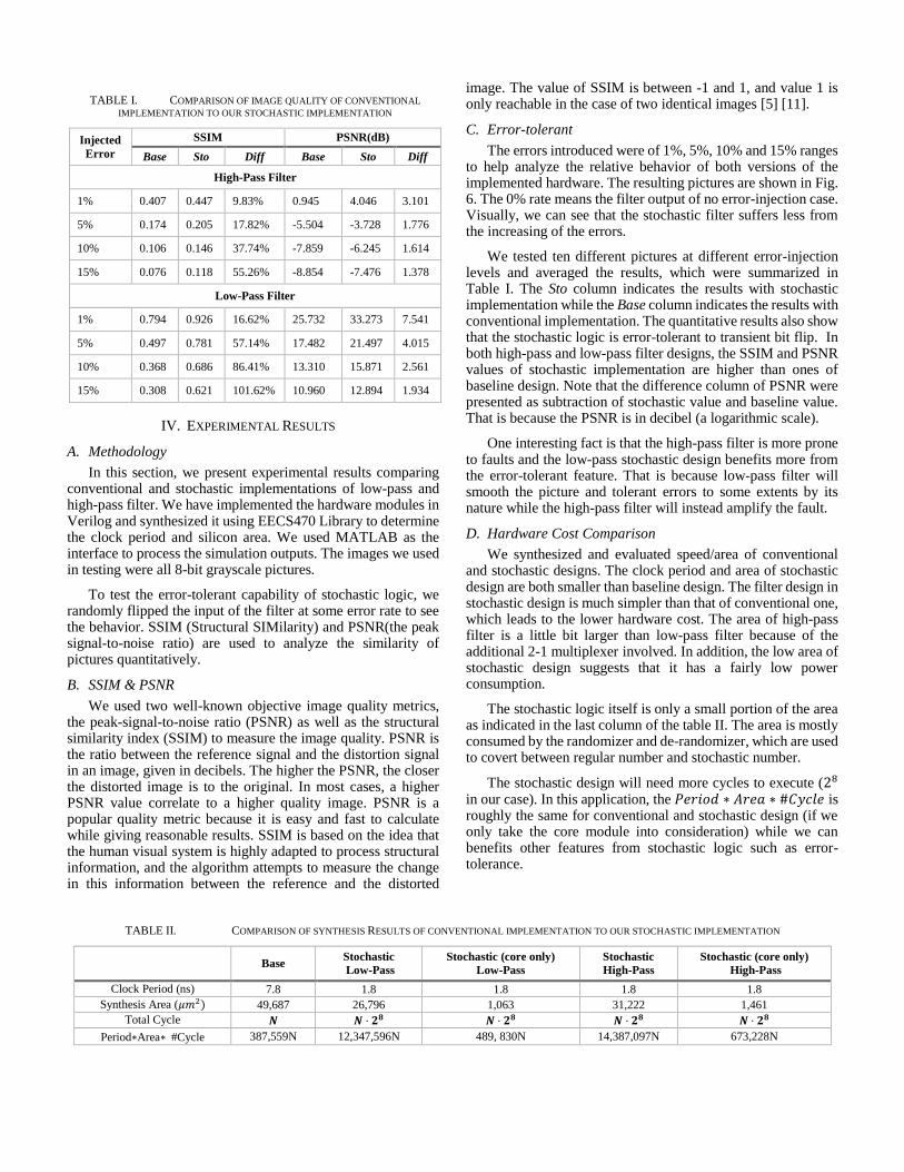
The errors introduced were of 1%, 5%, 10% and 15% ranges to help analyze the relative behavior of both versions of the implemented hardware. The resulting pictures are shown in Fig. 6. The 0% rate means the filter output of no error-injection case. Visually, we can see that the stochastic filter suffers less from the increasing of the errors.

We tested ten different pictures at different error-injection levels and averaged the results, which were summarized in Table I. The Sto column indicates the results with stochastic implementation while the Base column indicates the results with conventional implementation. The quantitative results also show that the stochastic logic is error-tolerant to transient bit flip. In both high-pass and low-pass filter designs, the SSIM and PSNR values of stochastic implementation are higher than ones of baseline design. Note that the difference column of PSNR were presented as subtraction of stochastic value and baseline value. That is because the PSNR is in decibel (a logarithmic scale).

One interesting fact is that the high-pass filter is more prone to faults and the low-pass stochastic design benefits more from the error-tolerant feature. That is because low-pass filter will smooth the picture and tolerant errors to some extents by its nature while the high-pass filter will instead amplify the fault.

D. Hardware Cost Comparison

We synthesized and evaluated speed/area of conventional and stochastic designs. The clock period and area of stochastic design are both smaller than baseline design. The filter design in stochastic design is much simpler than that of conventional one, which leads to the lower hardware cost. The area of high-pass filter is a little bit larger than low-pass filter because of the additional 2-1 multiplexer involved. In addition, the low area of stochastic design suggests that it has a fairly low power consumption.

The stochastic logic itself is only a small portion of the area as indicated in the last column of the table II. The area is mostly consumed by the randomizer and de-randomizer, which are used to covert between regular number and stochastic number.

The stochastic design will need more cycles to execute (28 in our case). In this application, the 𝑃𝑒𝑟𝑖𝑜𝑑 ∗ 𝐴𝑟𝑒𝑎 ∗ #𝐶𝑦𝑐𝑙𝑒 is roughly the same for conventional and stochastic design (if we only take the core module into consideration) while we can benefits other features from stochastic logic such as error-tolerance.

TABLE II. COMPARISON OF SYNTHESIS RESULTS OF CONVENTIONAL IMPLEMENTATION TO OUR STOCHASTIC IMPLEMENTATION

Base Stochastic

Low-Pass

Stochastic (core only)

Low-Pass

Stochastic

High-Pass

Stochastic (core only)

High-Pass

Clock Period (ns) 7.8 1.8 1.8 1.8 1.8

Synthesis Area (𝜇𝑚2) 49,687 26,796 1,063 31,222 1,461

Total Cycle 𝑵 𝑵 ⋅ 𝟐𝟖 𝑵 ⋅ 𝟐𝟖 𝑵 ⋅ 𝟐𝟖 𝑵 ⋅ 𝟐𝟖

Period∗Area∗ #Cycle 387,559N 12,347,596N 489, 830N 14,387,097N 673,228N

TABLE I. COMPARISON OF IMAGE QUALITY OF CONVENTIONAL

IMPLEMENTATION TO OUR STOCHASTIC IMPLEMENTATION

Injected

Error

SSIM PSNR(dB)

Base Sto Diff Base Sto Diff

High-Pass Filter

1% 0.407 0.447 9.83% 0.945 4.046 3.101

5% 0.174 0.205 17.82% -5.504 -3.728 1.776

10% 0.106 0.146 37.74% -7.859 -6.245 1.614

15% 0.076 0.118 55.26% -8.854 -7.476 1.378

Low-Pass Filter

1% 0.794 0.926 16.62% 25.732 33.273 7.541

5% 0.497 0.781 57.14% 17.482 21.497 4.015

10% 0.368 0.686 86.41% 13.310 15.871 2.561

15% 0.308 0.621 101.62% 10.960 12.894 1.934

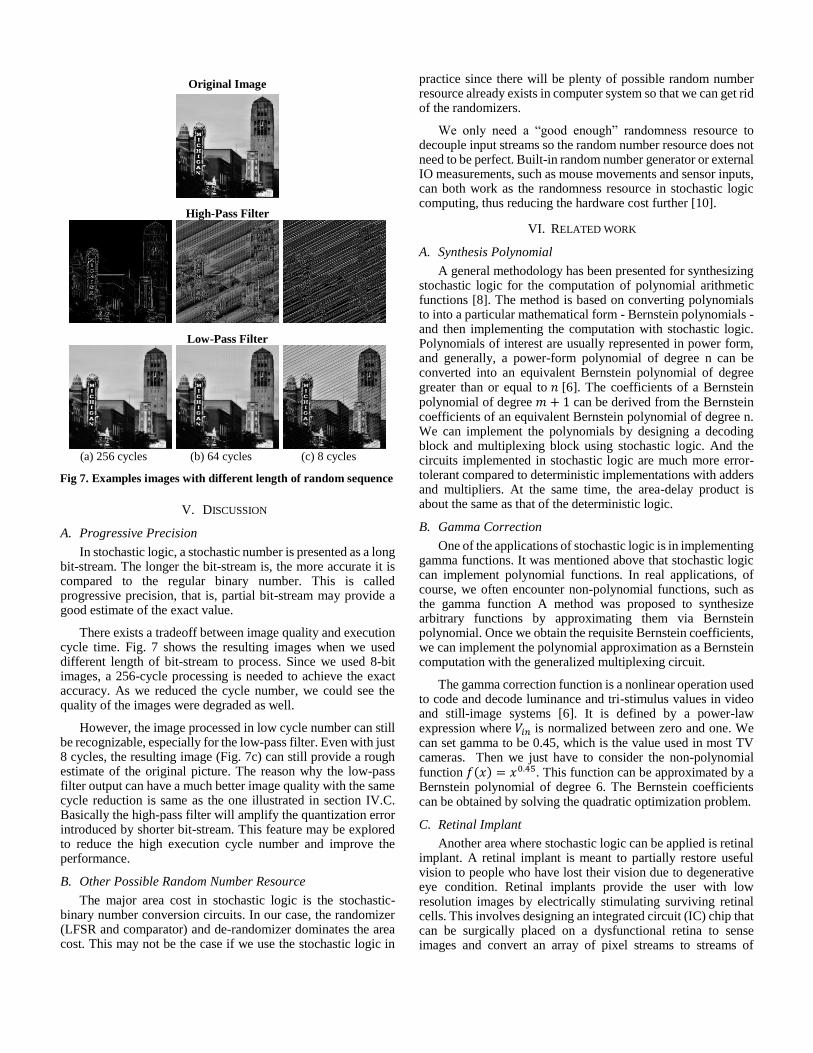
V. DISCUSSION

A. Progressive Precision

In stochastic logic, a stochastic number is presented as a long bit-stream. The longer the bit-stream is, the more accurate it is compared to the regular binary number. This is called progressive precision, that is, partial bit-stream may provide a good estimate of the exact value.

There exists a tradeoff between image quality and execution cycle time. Fig. 7 shows the resulting images when we used different length of bit-stream to process. Since we used 8-bit images, a 256-cycle processing is needed to achieve the exact accuracy. As we reduced the cycle number, we could see the quality of the images were degraded as well.

However, the image processed in low cycle number can still be recognizable, especially for the low-pass filter. Even with just 8 cycles, the resulting image (Fig. 7c) can still provide a rough estimate of the original picture. The reason why the low-pass filter output can have a much better image quality with the same cycle reduction is same as the one illustrated in section IV.C. Basically the high-pass filter will amplify the quantization error introduced by shorter bit-stream. This feature may be explored to reduce the high execution cycle number and improve the performance.

B. Other Possible Random Number Resource

The major area cost in stochastic logic is the stochastic-binary number conversion circuits. In our case, the randomizer (LFSR and comparator) and de-randomizer dominates the area cost. This may not be the case if we use the stochastic logic in

practice since there will be plenty of possible random number resource already exists in computer system so that we can get rid of the randomizers.

We only need a “good enough” randomness resource to decouple input streams so the random number resource does not need to be perfect. Built-in random number generator or external IO measurements, such as mouse movements and sensor inputs, can both work as the randomness resource in stochastic logic computing, thus reducing the hardware cost further [10].

VI. RELATED WORK

A. Synthesis Polynomial

A general methodology has been presented for synthesizing stochastic logic for the computation of polynomial arithmetic functions [8]. The method is based on converting polynomials to into a particular mathematical form - Bernstein polynomials - and then implementing the computation with stochastic logic. Polynomials of interest are usually represented in power form, and generally, a power-form polynomial of degree n can be converted into an equivalent Bernstein polynomial of degree greater than or equal to 𝑛 [6]. The coefficients of a Bernstein polynomial of degree 𝑚 + 1 can be derived from the Bernstein coefficients of an equivalent Bernstein polynomial of degree n. We can implement the polynomials by designing a decoding block and multiplexing block using stochastic logic. And the circuits implemented in stochastic logic are much more error-tolerant compared to deterministic implementations with adders and multipliers. At the same time, the area-delay product is about the same as that of the deterministic logic.

B. Gamma Correction

One of the applications of stochastic logic is in implementing gamma functions. It was mentioned above that stochastic logic can implement polynomial functions. In real applications, of course, we often encounter non-polynomial functions, such as the gamma function A method was proposed to synthesize arbitrary functions by approximating them via Bernstein polynomial. Once we obtain the requisite Bernstein coefficients, we can implement the polynomial approximation as a Bernstein computation with the generalized multiplexing circuit.

The gamma correction function is a nonlinear operation used to code and decode luminance and tri-stimulus values in video and still-image systems [6]. It is defined by a power-law expression where 𝑉𝑖𝑛 is normalized between zero and one. We can set gamma to be 0.45, which is the value used in most TV cameras. Then we just have to consider the non-polynomial function 𝑓(𝑥) = 𝑥0.45. This function can be approximated by a Bernstein polynomial of degree 6. The Bernstein coefficients can be obtained by solving the quadratic optimization problem.

C. Retinal Implant

Another area where stochastic logic can be applied is retinal implant. A retinal implant is meant to partially restore useful vision to people who have lost their vision due to degenerative eye condition. Retinal implants provide the user with low resolution images by electrically stimulating surviving retinal cells. This involves designing an integrated circuit (IC) chip that can be surgically placed on a dysfunctional retina to sense images and convert an array of pixel streams to streams of

Original Image

High-Pass Filter

Low-Pass Filter

(a) 256 cycles (b) 64 cycles (c) 8 cycles

Fig 7. Examples images with different length of random sequence

neural-style electrical signals that stimulate useful visual sensations.

Due to the fact that stochastic logic can handle streaming analog data, process the data digitally and has good noise tolerance, it has the potential to meet most of the challenging requirements of the retinal implant application: streaming neural-style data, very small circuit size, extremely low power and insensitivity to noise. For example, in the retinal implant application, a real-time edge-detecting circuit generates high-contrast images of the environment that greatly help a vision-impaired person to navigate correctly and avoid obstacles. The stochastic logic circuit can be designed in a high efficient way to meet this requirement [1].

VII. CONCLUSION

In this paper, we presented our implementation of low-pass (smoothing) and high-pass (sharpening) filters in stochastic logic. We found that stochastic logic filters can operate at a faster clock frequency and consume less silicon area than conventional filter design. While it will take more cycles to process one pixel, stochastic logic takes advantage of randomness to make the filter error tolerant and more reliable. In the future, more efforts are needed to minimize the hardware cost of conversion circuits.

ACKNOWLEDGEMENTS

We thank Professor Bertacco and Dr. Doowon Lee for providing guidance and assistance in our project. This project is motivated by the slides from course EECS 478, taught by Professor John P. Hayes.

REFERENCES

[1] A. Alaghi, C.Li and J. P. Hayes. Stochastic circuits for real-time image-processing applications. In Proceedings of the 50th Annual Design Automation Conference (p. 136). ACM. May. 2013.

[2] M. Alioto, G. Palumbo and M. Pennisi. Understanding the effect of process variations on the delay of static and domino logic. Very Large Scale Integration (VLSI) Systems, IEEE Transactions on, 18(5), 697-710, 2010.

[3] B. D. Brown and H. C. Card. Stochastic neural computation. I. Computational elements. Computers, IEEE Transactions on, 50(9), 891-905, 2001.

[4] V. A. Chandrasetty. VLSI Design: A Practical Guide for FPGA and ASIC Implementations. Springer Science & Business Media. 17-46, 2011.

[5] A. Hore and D. Ziou (2010, August). Image quality metrics: PSNR vs. SSIM. In Pattern Recognition (ICPR), 2010 20th International Conference on (pp. 2366-2369). IEEE, Aug. 2010.

[6] P. Li, W. Qian and D. J, Lilja. A stochastic reconfigurable architecture for fault-tolerant computation with sequential logic. In Computer Design (ICCD), 2012 IEEE 30th International Conference on, 303-308, IEEE, Sep. 2012.

[7] W. Qian, X. Li, M. D. Riedel, K. Bazargan and D. J. Lilja. An architecture for fault-tolerant computation with stochastic logic. Computers, IEEE Transactions on, 60(1), 93-105, 2011.

[8] W. Qian and M. D. Riedel. The synthesis of robust polynomial arithmetic with stochastic logic. In Design Automation Conference, 2008. DAC 2008. 45th ACM/IEEE (pp. 648-653). IEEE, Jun.2008.

[9] K. B. R. Teja, A. S. Warrier, A. S. Belvadi and D. R. Gawhane. Design and implementation of neighborhood processing operations on FPGA using verilog HDL. IOSR Journal of VLSI and Signal Processing, 4(1), 75-80, 2014.

[10] J. Ortega, C. Janer, J. Quero, L. Franquelo, J. Pinilla, and J. Serrano,“Analog to digital and digital to analog conversion based on stochastic logic,” in International Conference on Industrial Electronics, Control, and Instrumentation, 1995, pp. 995–999

[11] Y. B. Tong, Q. S. Zhang and Y. P. Qi. Image quality assessing by combining PSNR with SSIM. Journal of Image and Graphics, 12, 1758-1763, 2006.