Error Squares

8/11/2019 Error Squares

http://slidepdf.com/reader/full/error-squares 1/26



Linea r Least Sq uares

Approximatio n

ByKristen Bauer, Renee Metzger,

Holly Soper, Amanda Unklesbay

http://muskingum.facebook.com/photo.php?pid=47629&id=566420623&op=1&view=all&subj=82001515








http://muskingum.facebook.com/photo.php?pid=30273604&id=82000852&op=1&view=user&subj=82000852



Linear Least Squares

Is the line of best fitfor a group of points

It seeks to minimizethe sum of all datapoints of the squaredifferences between

the function value anddata value.

It is the earliest form

of linear regression

http://www.vias.org/science_cartoons/thumbnails.html



Gauss and Legendre

The method of least squares wasfirst published by Legendre in1805 and by Gauss in 1809.

Although Legendre’s work waspublished earlier, Gauss claimshe had the method since 1795.Both mathematicians applied the

method to determine the orbits ofbodies about the sun.Gauss went on to publish furtherdevelopment of the method in

1821.

http://upload.wikimedia.org/wikipedia/commons/9/9b/Carl_Friedrich_Gauss.jpg



ExampleConsider the points (1,2.1) , (2,2.9) , (5,6.1) , and (7,8.3) with the best fit line f(x) = 0.9x + 1.4

The squared errors are:x1=1 f(1)=2.3 y 1=2.1 e 1= (2.3 – 2.1)² = .04

x2=2 f(2)=3.2 y 2=2.9 e 2= (3.2 – 2.9)² =. 09x3=5 f(5)=5.9 y 3=6.1 e 3= (5.9 – 6.1)² = .04x4=7 f(7)=7.7 y 4=8.3 e 4= (7.7 – 8.3)² = .36

So the total squared error is .04 + .09 + .04 + .36 = .53

By finding better coefficients of the best fit line, we can make this errorsmaller…



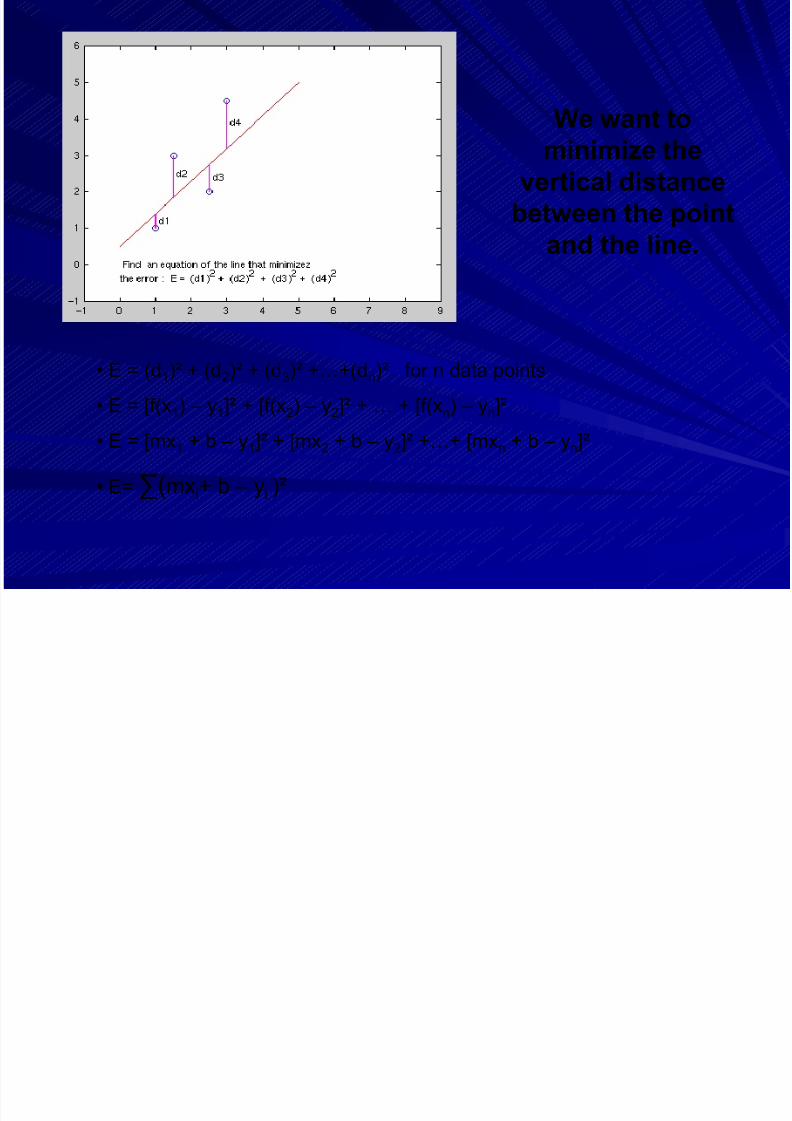
We want tominimize the

vertical distancebetween the point

and the line.

• E = (d 1)² + (d 2)² + (d 3)² +…+(d n)² for n data points

• E = [f(x 1) – y1]² + [f(x 2) – y2]² + … + [f(x n) – yn]²• E = [mx 1 + b – y1]² + [mx 2 + b – y2]² +…+ [mx n + b – yn]²

• E= ∑(mx i+ b – y i )²



E must be MINIMIZED!

How do we do this?E = ∑(mx i+ b – y i )²

Treat x and y as constants, since we aretrying to find m and b.So…PARTIALS!

E/ m = 0 and E/ b = 0But how do we know if this will yieldmaximums, minimums, or saddle points?



Minimum Point Maximum Point

Saddle Point



Minimum!

Since the expressionE is a sum ofsquares and istherefore positive (i.e.it looks like an upwardparaboloid), we knowthe solution must be aminimum.We can prove this byusing the 2 nd PartialsDerivative Test.



2nd Partials Test

And form the discriminant D = AC – B2

1) If D < 0, then (x 0,y0) is a saddle point .2) If D > 0, then f takes on

A local minimum at (x 0,y0) if A > 0

A local maximum at (x 0,y0) if A < 0

A f x

B f y x

C f y

2

2

2 2

2, ,

Suppose the gradient of f(x 0,y0) = 0.(An instance of this is E/ m = E/ b = 0.)

We set



Calculating the Discriminant

A f

x

A E

m

Amx b y

m

A x mx b y

m A x

A x

2

2

2

2

2 2

2

2

2

2

2

2

( )

( )( )

( )

B f

y x

B E

b m

Bmx b y

b m

B x mx b y

b B x

B x

2

2

2 2

2

2

2

( )

( )( )

( )

C f

y

C E

b

C mx b y

b

C mx b y

bC C

2

2

2

2

2 2

2

2

22 1

( )

( )( )

D AC B x x 2 2 24 1 4( ( ))



1) If D < 0, then (x 0,y0) is a saddle point .2) If D > 0, then f takes on

A local minimum at (x 0,y0) if A > 0 A local maximum at (x 0,y0) if A < 0

Now D > 0 by an inductive proof showing that

Those details are not covered in thispresentation.We know A > 0 since A = 2 ∑ x2 is always

positive (when not all x’s have the same value).

D AC B x x 2 2 24 1 4( ( ))

n x xi

n

ii

n

i

1

2

1

2



Therefore…

Setting E/ m and E/ b equal to zero will

yield two minimizing equations of E, thesum of the squares of the error.

Thus, the linear least squares algorithm(as presented) is valid and we can continue.



E = ∑(mx i + b – y i)² is minimized (as just shown) whenthe partial derivatives with respect to each of thevariables is zero. ie: E/ m = 0 and E/ b = 0

E/ b = ∑2(mx i + b – y i) = 0 set equal to 0m∑x i + ∑b = ∑y i

mSx + bn = SyE/ m = ∑2x i (mx i + b – y i) = 2∑(m xi² + bx i – x iyi) = 0

m∑xi² + b ∑x i = ∑x iyi

mSxx + bSx = Sxy

NOTE:∑x i = Sx ∑y i = Sy ∑x i² = Sxx ∑x iyi = SxSy



Next we will solve the system ofequations for unknowns m and b:

nmSxx + bnSx = nSxy Multiply by nmSxSx + bnSx = SySx Multiply by Sx

nmSxx – mSxSx = nSxy – SySx Subtract

mSxx bSx SxymSx bn Sy

mnSxy SySxnSxx SxSx

m(nSxx – SxSx) = nSxy – SySx Factor m

Solving for m…



Next we will solve the system ofequations for unknowns m and b:

mSxSxx + bSxSx = SxSxy Multiply by SxmSxSxx + bnSxx = SySxx Multiply by Sxx

bSxSx – bnSxx = SxySx – SySxx Subtract

mSxx bSx SxymSx bn Sy

bSxxSy SxySxnSxx SxSx

b(SxSx – nSxx) = SxySx – SySxx Solve for b

Solving for b…



Example: Find the linear least squaresapproximation to the data: (1,1), (2,4), (3,8)

mnSxy SySxnSxx SxSx

Sx = 1+2+3= 6Sxx = 1²+2²+3² = 14Sy = 1+4+8 = 13Sxy = 1(1)+2(4)+3(8) = 33n = number of points = 3

The line of best fit is y = 3.5x – 2.667

Use these formulas:

bSxxSy SxySxnSxx SxSx

b

14 13 33 63 14 6 6

166

2667( ) ( )( ) ( )

.

m

3 33 6 133 14 6 6

216

35( ) ( )( ) ( )

.



Line of best fit: y = 3.5x – 2.667

-1 1 2 3 4 5

-5

5

10

15



THE ALGORITHM

in Mathematica







ActivityFor this activity we are going to use the linear leastsquares approximation in a real life situation.You are going to be given a box score from either abaseball or softball game.With the box score you are given you are going to writeout the points (with the x coordinate being the number ofhits that player had in the game and the y coordinatebeing the number of at-bats that player had in the game).

After doing that you are going to use the linear leastsquares approximation to find the best fitting line.The slope of the besting fitting line you find will be theteam’s batting average for that game.



In Conclusion…

E = ∑(mx i+ b – y i )² is the sum of thesquared error between the set of datapoints {(x1,y1),…,(x i,y i),…,(x n,yn)} and theline approximating the data f(x) = mx + b .By minimizing the error by calculusmethods , we get equations for m and bthat yield the least squared error :

mnSxy SySxnSxx SxSx

b

SxxSy SxySxnSxx SxSx



Advantages

Many common methods of approximating dataseek to minimize the measure of differencebetween the approximating function and givendata points.

Advantages for using the squares of differencesat each point rather than just the difference,absolute value of difference, or other measures oferror include: – Positive differences do not cancel negative differences – Differentiation is not difficult – Small differences become smaller and large differences

become larger



Disadvantages

Algorithm will fail if data points fall in avertical line.

Linear Least Squares will not be the bestfit for data that is not linear.






http://slidepdf.com/reader/full/error-squares 26/26Th E d








Documents

Error Squares