Error estimation of paired comparison tests for Thurstone’sCase VPeter Zolliker, Zofia Baranczuk, Laboratory for Media Technology; Swiss Federal Laboratory for Materials Testing and Research(EMPA), Duebendorf

AbstractPair comparison methods based on Case V of Thurstone’s

Law of Comparative Judgment are widely used to derive intervalscales for perceptual image quality. A thorough treatment of theinvolved statistical errors is often neglected, even though this isthe base for computing confidence intervals and other statisticaltests. In this paper we show, that consequent error estimationthrough all steps of the data analysis provides a simple and reli-able method to compute confidence intervals. Monte Carlo simu-lations are used to verify the results and to compare the proposederror estimation with other known methods.Keywords: paired comparison, Thurstone’s Law of ComparativeJudgment, error estimation

IntroductionPsycho-visual tests are used for subjectively evaluating the

quality of images. A typical example is the measurement ofthe quality of images transformed by gamut mapping algorithms.There are a variety of methods to carry out such tests. The aimof the tests is to compare images with respect to perceived qual-ity. Often an interval scale for the different variants of an imageis computed from these comparisons, where a scale value is ameasure for the relative quality of a specific image variant. Forone important application, namely gamut mapping, CIE guide-lines for algorithms [1] provide specific experimental methods,viewing conditions, and reference algorithms. Three kinds ofpsycho-visual tests are recommended for evaluating the qualityof gamut mapping algorithms: pair comparison, rank order, andcategory judgment. The most widely used method is pair com-parison. It is also the easiest for the observers, especially if thedifferences between the images are small.

A pair of images from a set A is presented to an observer.He or she is then asked to choose the one that better fulfills in-structions of the test. In the gamut mapping case, the instructionsusually state that one should choose the more aesthetic image, orthe image more similar to the original. In the latter case the orig-inal image is shown along with the transformed images.

A thorough treatment of the involved statistical errors is of-ten neglected, even though this is the base for computing confi-dence intervals. Morovic [2] gives a simple formula to estimateconfidence intervals. The formula depends only on the number ofobservations N per pair of stimuli but not on the number of stim-uli n. Since then this method seems to have been used in manypsycho-visual studies on gamut mapping. Only a few of themcite the used formula explicitly [3]. The CIE-guidelines [1] givea reference to Morovic’s thesis concerning confidence intervalsof paired comparison.

In a recent paper Montag [4] has investigated the problemof missing dependency on the number of stimuli n using MonteCarlo simulations. He derived an empirical formula showing ap-proximate dependency of the estimated error with the square rootof the product of N as well as and n. Newer gamut mapping stud-

ies have used this formula for error estimation [5]. Older stan-dard books on psycho-visual scaling [6, 7] give more detaileddescription for error estimations, however their results are tied totheir specific data analysis and a direct application to the standardevaluation of the Thurstone’s Case V is not obvious.

In this paper we will give a direct derivation of error esti-mation for Thurstone’s Case V. It is based on error propagation.We will use Monte Carlo simulations to compare the results withother commonly used methods and to find the region of applica-bility as a function of the number of observations N the numberof stimuli n and scale value range.

MethodologyThurstone’s Law of Comparative Judgment

Thurstone’s Law of Comparative Judgment is a methodused for evaluating data obtained in a pair comparison test [8].It falls into the class of discrete choice models. We consider onlyCase V, i.e. that the discriminal differences follow a Gaussian dis-tribution of equal width and that there is no correlation betweentwo stimuli. For our methodology we leave it open, whether apair comparison test was made by one or several observers. Wealso ignore whether a single image or several images were usedin the test. However we make the rather strong assumption, thatall judgments are independent of a specific observer and image.Furthermore we assume forced choice for the pair comparisontest to avoid treatment of tie choices.

Given a set A of n stimuli, e.g. gamut mapping algorithms,and choice data of the form i� j with i, j ∈ A. We know the fre-quency fi j (F-matrix) of stimulus i being preferred over stimulusj (number of times i is preferred over j). We consider the propor-tion qi j (Q-matrix) of stimulus i being preferred over stimulus jdefined by

qi j =fi j +δ

fi j + f ji +2δ(1)

as an indirect measure for the distance of the “qualities” (namedscale values) vi of i and v j of j, respectively. We introduced thebias correction δ in order to eliminate numerical problems forpairs of items, which have zero entries in the frequency matrix.Except where stated we used in this paper δ = 0.2. For a discus-sion of different bias correction formulae see also Engeldrum [9,chapter 9.4].

Discrete choice models build on the assumption that theobserved choices are outcomes of random trials: confrontedwith the two options i, j ∈ A an observer assigns quality valuesui = vi + εi and u j = v j + ε j, respectively, to the stimuli, wherethe error terms εi and ε j are drawn independently from the samedistribution. The observer then prefers the stimulus with largerquality value. Hence the probability pi j that i is preferred over jis given as

pi j = Pr[ui ≥ u j]

= Pr[vi + εi ≥ v j + ε j] = Pr[vi− v j ≥ ε j− εi].

CGIV 2010 Final Program and Proceedings 39

In Thurstone’s model [8] the error terms εi are drawn froma normal distribution N(0,σ2). Thurstone’s Case V model as-sumes that the variances for all stimuli are equal. The differenceε j − εi is also normally distributed with expectation 0 and vari-ance 2σ2 and thus

pi j = Pr[ui ≥ u j] = Pr[vi− v j ≥ ε j− εi]

= Φ

(vi− v j√

2σ

),

where Φ is the cumulative distribution function of the standardnormal distribution

Φ(x) =1√2π

∫ x

−∞

e−y2/2dy.

This is equivalent to

vi− v j =√

2σΦ−1(pi j). (2)

Let us notice, that qi j is an empirical approximation of pi j.Using the proportion qi j of i being preferred over j we set

zi j = Φ−1(qi j) [Z−matrix]. (3)

Note, that the Z-matrix is antisymmetric, thus zi j = −z ji.Mosteller [10] has already mentioned that the least squares so-lution of the system of equations for the scale values vi can bedetermined by averaging the columns

vi =1n

√2σ ∑

jzi j. (4)

In order to fix the arbitrary offset of the scale values, the sum ofall scale values vi is assumed to be zero.

Error estimation.In order to gauge the statistical significance of differences

between scale values as well as for statistical tests a good errorestimation is needed. In this paper consider the estimated stan-dard deviation of a value as the estimated error of that value.These estimated errors serve as a basis for the calculation ofconfidence intervals and other statistical tests such as χ2-tests.Typical applications are model verification using Mosteller’s Testor the testing whether scale values from different data sets (e.g.expert versus general observers) are statistically indistinguish-able. There are a few known methods for estimating errors forthe Thurstone Case V, which will be described in the following.

Morovic’s error estimation. Morovic [2, chapter 4] gives thefollowing formula to estimate the 95 per cent confidence interval:

CIS = 1.96σ√N

. (5)

With σ = 1/√

2 we can compute the underlying estimated stan-dard deviation for the scale values

Em =

√1

2N(6)

Montag’s error estimation. Montag [4] has published an em-pirical formula for the estimated standard deviation of scale val-ues based on Monte Carlo simulations.

Ee = b1(n−b2)b3(N−b4)b5 (7)

with b1 = 1.76, b2 = −3.08, b3 = −0.613, b4 = 2.55 and b5 =−0.491. It shows the expected approximate dependency of theestimated error with the square root of the product of N and n(b3 ≈−0.5 and b5 ≈−0.5).

Analytic error estimation. Here we derive an analytic errorestimate for Thurstone’s method. The basic approach is to es-timate the error in the image choice process and then propagat-ing the error through the data evaluation steps: This process ofchoosing one image from the pair of images can be modeled asa Bernoulli trial with success probability pi j. The standard de-viation for pi j equals to the standard deviation for a Bernoullivariable in N trials

σpi j =

√pi j(1− pi j)

N(8)

As we approximate pi j by the empirical value qi j the es-timated error Eqi j for the proportion qi j in equation (1) can bewritten as

Eqi j = σqi j =

√qi j(1−qi j)

fi j + f ji +2δ. (9)

To compute the errors of the entries zi j in the Z matrix, wepropagate the error using equation (3)

Ezi j = Eqi j

ddqi j

Φ−1(qi j). (10)

Using equation (4) the errors of the scale values vi are com-puted as

Evi =1n

√2σ

√∑

b∈A;a6=bE2

zi j. (11)

Approximation of errors. An approximate error estimate canbe derived for Thurstone’s Case V if the probabilities pi j are notfar from 1/2. Then their standard deviation is

Eqi j ≈ const =

√1

4N(12)

and the error of the Z-matrix elements zi j can be approximatedas

Ez ≈√

14N

ddq

Φ−1(q) (13)

for q = 0.5 yielding

Ez ≈√

π

2N(14)

independent off i and j. Assuming σ = 1/√

2 the error forthe scale values vi is approximatively

Ev ≈1n

√π(n−1)

N(15)

independent on i. This formula shows also the expected approx-imate dependency of the estimated error with the square root ofthe product of N and n if n is not too small.

Experimental error estimation. Experimental error estima-tion [11] is an approach complementing above methods. It isbased on a minimum of assumptions. It samples the error bydividing the choice data randomly into two groups. For bothgroups scale values are individually computed and errors are es-timated from the differences of the values obtained from bothgroups. This process is repeated several times and the resultsare averaged to increase the accuracy of the error estimation. Ifall model assumption are fulfilled this error estimation should

40 ©2010 Society for Imaging Science and Technology

0

0.05

0.1

0.15

0.2

0.25

0 10 20 30 40 50 60 70

Number of observations N

err

or

es

tim

ati

on

fo

r s

ca

le v

alu

es

E_v

E_e

E_m

E_s (δ=0.1)

E_s (δ=0.5)

n=4n=7n=10n=15

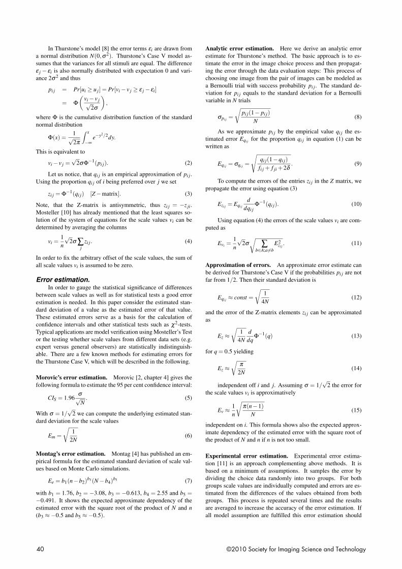
Figure 1. Simulated scale value errors ES compared to error error estimates Em (eq. 6), Ee (eq. 7) and Ev (eq 15) for different number of stimuli. Triangles

and circles are for simulated errors and lines are for estimated errors.

within the statistics deliver the same error as the one obtainedfrom analytic error estimation.

A special option of this method is to test the heterogeneityamong the observers (or among the individual images). In thiscase individual observers (or individual images) are randomly di-vided into two groups and errors are computed from the averagedifference of the scale values between the two groups. Here er-ror estimation using such biased samplings allows to test whetherthe choices depend on individual observers (or images).

Relation of error propagation with Mosteller’stest.

Based on the error estimation Eqi j the error of the arcsinetransformed scale values θi j = arcsin(2qi j − 1) can be derivedusing error propagation

Eθ i j = Eqi j

ddqi j

arcsin(2qi j−1)) (16)

Using equation (9) and the derivative of arcsin the errors ofthe θi j values simplify to

Eθ i j =

√qi j(1−qi j)

N

√1

qi j(1−qi j)=

1√N

(17)

This result confirms the usefulness of the arcsine transfor-mation in Mosteller’s χ2 test. With this transformation the vari-ance of the θ -values is independent of the proportion qi j and de-pends only on the number of observations N.1 Thus estimation

1Note, that if we want to find a transformation which has the propertyof equalizing the standard deviation of all probability values pi j based oneq. (8) we end up with an arcsine function.

of errors and confidence intervals based on the arcsine transfor-mation can be linked to the error estimation of the scale valuesby error propagation.

SimulationWe used Monte Carlo simulation in order to compare the

different error estimations and to investigate their validity as afunction of the number of observation N, the number of stimuli nand the scale value range. For all simulations we assumed a psy-chological continuous scale that conforms to Thurstone’s CaseV, i.e., that the discriminal differences follow a Gaussian distri-bution of equal width and that no correlation exist between twostimuli i and j. Furthermore we assumed no correlation neitherin the responses of an individual observer nor in responses foran individual image. Thus ideal conditions are assumed for thesimulated experiments.

Simulation for small scale valuesThe first series of simulation experiments was set up to com-

pare the analytic error estimation with the estimation and sim-ulation given in Montag’s [4] article. We used the followingnumber of stimuli n = [4,7,10,15]. The number N of observa-tions per pair of stimuli was in the range of [10...60]. We usedstimuli with small scale value differences compared to the widthof the distribution of the discriminal process. Thus the n scalevalues were assumed to be uniformly distributed in the range[−0.25... + 0.25]. Each experiment was repeated 10’000 timesfor each combination of parameters. The simulated error Es ofthe scale values was calculated using the standard deviation ofthe scale values from the experiments. Furthermore it was veri-

CGIV 2010 Final Program and Proceedings 41

fied, that the average scale values extracted from the simulationcompare to the scale value of the model with an accuracy wellwithin the error estimation. Three different values for the biascorrection were used in the simulation (δ = 0.1, 0.2 and 0.5).

In Fig. 1 the experimental error Es is compared to the errorestimates Em (eq. 6), Ee (eq. 7) and Ev (eq. 15). The error Emgenerally overestimates the simulated error Es. The overestima-tion increases with the number n of stimuli. The error estimatesEe and Ev are in good agreement with the simulated error for allinvestigated combinations of n and N and compare well with theresults given by Montag [4]. The differences between Ee and Evget smaller with higher N. For small N the differences are in thevariability range of different bias correction values δ . Simulatederrors using a bias correction δ = 0.1 follows Montag’s error es-timation Ee, where a use of δ = 0.5 is in good agreement withEv.

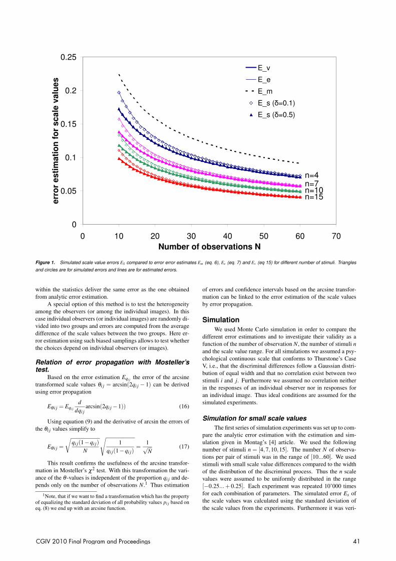
Error simulation for individual scale valuesThe estimated error Evi in eq. (11) depends on the scale

value. This dependency gets important as soon as the percentagesqi j differ substantially from 0.5. In a second series of simulationexperiments this dependency has been investigated. We used thefollowing parameters: The number of stimuli was n = [4,8,16],the n scale values were assumed to be uniformly distributed in therange [−1.0...+1.0]. The number of observations was fixed to arather large number N = 200 to avoid a significant influence ofbias corrections. The result is shown in Fig. 2. Each experimentwas repeated 10’000 times for each combination of parameters.

0

0.02

0.04

0.06

0.08

0.1

-1 -0.5 0 0.5 1

scale value

es

tim

ate

d e

rro

r

E_vi (n=16) E_s (n=16) E_v (n=16)

E_vi (n=8) E_s (n=8) E_v (n=8)

E_vi (n=4) E_s (n=4) E_v (n=4)

E_m

Figure 2. Simulated scale value errors as a function of z-scale compared

to error estimations for different number of stimuli. squares and circles are

for simulated errors, full lines for estimated errors Evi , dashed lines for Em

and Ev.

The simulated error Es is increasing with higher absolutescale values. This increase is nicely reproduced by the error es-timation Evi given in eq. (11). The error approximation Ev canbe regarded as a lower limit for the simulated error. The same is

true for Ee which, for this high number N, is basically identicalto Ev.

Accuracy of error estimationA third series of simulation experiments has been performed

to test the accuracy of the four error estimations Em, Ee, Ev andEvi as a function of N, n and the scale value range. For thispurpose we investigate the relative accuracy in percentage of theerror compared to the simulated error. Within one specific exper-iment the maximum relative deviation of an estimated error fromthe simulated error was taken as a measure for the accuracy ofan estimated error. 40 different scale value ranges were used upto [−2.0...2.0], N was in the range [2..100] in steps of 2 and thenumber of stimuli n was [3,4,5,8,12,16]. For each experimentscale values for n stimuli were selected as follows: n values xiwere randomly chosen in the range [−1.0...+ 1.0]. Then thesevalues were scaled such that the difference between the mini-mum and maximum scale corresponded to the target scale valuerange. For each combination of N, n and scale value ranges theexperiment was repeated at least 2000 times and simulated errorsEs, average scale value errors Evi , approximate errors Em and Eewere calculated. In Fig. 3 we show the results for 3, 5 and 8stimuli.

The error estimation Em is accurate in a range of 20% onlyfor n = 3. It is not accurate for larger number of stimuli. Thisconfirms, that the error estimation Em should, if at all, be usedonly for a small number of stimuli, i.e. smaller than five. Theerror estimations Ee and Ev have regions with high accuracy forall numbers of stimuli, but only for small and moderate scalevalues up to about 1.0. For these scale value ranges, the errorestimation for all scale values are approximately equal and Ee(as well as Ev) give a simple, quick and accurate error estimation.The best error estimation is given by Evi . The accuracy is betterthan 10% for all number of stimuli n and number of observationsN up to a limiting scale value range. The limiting scale valuerange basically scales with the square root of N. The limit isreached when one or more expected fi j in the frequency matrixare close to or smaller than one. Interestingly the accuracy of theerror estimations Ee, Evi and Ev depend only marginally dependon the number of stimuli n.

DiscussionThe simple error estimation given by Morovic [2] gener-

ally overestimates the error and is approximately correct only forsmall number of stimuli (n≈ 3...4). It is not suitable as a generalerror estimation method.

For many cases the error approximation Ev as well as theempirical error estimation Ee given by Montag [4] are sufficientlyaccurate. The advantage of deriving the error approximation an-alytically (as for Ev and Evi ) is, that an adaption to other dis-criminal distributions such as the logistic distribution of Bradley-Terry [12] is straightforward. The inverse cumulative distributionfunction Φ−1 and its derivative in equations (3), (10) and (14)have to be replaced by the appropriate functions. Furthermorenote that an empirical formula is always restricted to the param-eter range used in the fitting process. It is questionable, whetherthe formula given by Montag can be extended to n < 4 or to largeN. It will even fail for the (trivial) case of n = 2, because the pa-rameter b4 is larger then 2.

From Fig. 3 we can define a validity range of error estima-tion if we assume some limit for the accuracy. It is reasonableto assume that error estimation has to be accurate to 10%. Thenthe approximative errors Em (eq. 7) and Ev (eq. 15) are good ap-

42 ©2010 Society for Imaging Science and Technology

proximations for all large enough number N of observation, aslong as the range of the scale values is small enough. The upperlimit for the scale value range for large N is just above 1.0. Thevalidity range of the error estimation Evi extends to much higherscale value range. The limiting factor of this error estimation isthe expected number of judgments for the least probable entry inthe frequency matrix fi j. This is due to the fact that the entriesin the Z-matrix column zi j are averaged and the error of the en-try with the highest error also has the highest contribution to theerror of the scale value vi. A weighted linear regression methodsuch as described by Bock and Jones [6, chapter 6] could givemore accurate scale values with smaller estimated errors in thecase of a large scale value range. For these cases the proposederror estimation Evi has reached its limit.

In all our simulations we assumed the ideal Case V of Thur-stone’s Law of Comparative Judgment. Note that besides ac-curate computation of scale values also the estimation of theirerror is valid only if the underlying assumptions are valid. Forexample, if Mosteller’s test fails the error estimation must alsobe questioned. Furthermore, correlations within individual ob-servers’ choices or within individual images have to be tested forexample by using experimental error estimation [11]. If enoughdata is available for individual observers, a comparison of intra-observer errors with inter-observer error estimations [2] can alsobe used to verify whether such correlations have to be taken intoaccount. The latter method can also be adapted to compare intra-image errors with inter-image errors.

ConclusionWe have shown, that analytic error estimation using error

propagation gives good results for data evaluation of psycho-visual data using Thurstone Case V. The effort for this errorcomputation is as small as the computation of the scale valuesthemselves. This error estimation method should replace previ-ous methods because it can be applied for a much larger rangeof psycho-visual scales. The simulation was based on an idealThurstone Case V model. Future simulations including corre-lations among individual users or individual images could givefurther insight to improve error estimation.

AcknowledgmentsPart of this research was supported by the Hasler Stiftung

Proj. # 2200.

References[1] Central Bureau of the CIE, Vienna. CIE Publication 156: Guide-

lines for the Evaluation of Gamut Mapping Algorithms, 2004.[2] J. Morovic. To Develop a Universal Gamut Mapping Algorithm.

PhD thesis, University of Derby, UK, 1998.[3] J. Y. Hardeberg, E. Bando, and M. Pedersen. Evaluating colour

image difference metrics for gamut mapping images. ColorationTechnology, 124(4):243–253, July 2008.

[4] E. D. Montag. Empirical formula for creating error bars for themethod of paired comparison. Journal of Electronic Imaging,15(1):010502 1–3, 2006.

[5] F. Dugay, I. Farup, and J. Y. Hardeberg. Perceptual evaluation ofcolor gamut mapping algorithms. Color Research and Application,33(6):470–476, 2008.

[6] R. D Bock and L. V. Jones. The measurement and Prediction ofJudgment and Choice. Holden-Day, San Francisco, 1968.

[7] H. A. David. The method of paired comparison. Hafner Press, NewYork, 1969.

[8] L Thurstone. A law of comparative judgement. In PsychologicalReview, pages 273–286, 1927.

[9] Peter G. Engeldrum. Psychometric Scaling, A Toolkit for ImagingSystems Development. Imcotek Press, Winchester MA, USA, 2000.

[10] F. Mosteller. Remarks on the method of paired comparisons: I. theleast squares solution assuming equal standard deviations and equalcorrelations. Psychometrika, 16:3, 1951.

[11] P. Zolliker, Z. Baranczuk, Sprow I., and Giesen J. Conjoint analy-sis used for the evaluation of parameterized gamut mapping algo-rithms. IEEE Transactions in Image Proceeding, 19(3):758–769,March 2010.

[12] R. A. Bradley and M. E. Terry. Rank analysis of incomplete blockdesigns, I. the method of paired comparisons. Biometrika, 39(3-4):324–345, 1952.

Author BiographyPeter Zolliker received a degree in physics from the ETH

Zurich, and the Ph.D. degree in crystallography from the Uni-versity of Geneva, Switzerland, in 1987. After two post-doc yearsat the Brookhaven National Laboratory he was a member of theR&D team at Gretag Imaging, working on image analysis, imagequality, setup, and color management procedures for analog anddigital printers. In 2003, he joined the EMPA, where his researchis focused on digital imaging and psychophysics.

Zofia Baranczuk received her bachelor’s degree in computerscience and master’s degree in mathematics from the WarsawUniversity. She works now on her doctorate and is engaged inpsycho-visual tests and gamut-mapping.

CGIV 2010 Final Program and Proceedings 43

Figure 3. Accuracy map of error estimation methods Em (top), Ee (upper middle), Ev (lower middle) and Evi (bottom) for number of stimuli n = 3 (left column),

n = 5 (middle column) and n = 8 (right column). Number N of observations is on vertical axis and scale value range on horizontal axis. Regions with an error

estimation accuracy better than 10% are shown in white, those between 10% and 20% in gray and accuracies worse than 20% in black.

44 ©2010 Society for Imaging Science and Technology