Embed Size (px)
Citation preview

Error Control for Network Coding
by
Danilo Silva
A thesis submitted in conformity with the requirementsfor the degree of Doctor of Philosophy
Graduate Department of Electrical and Computer EngineeringUniversity of Toronto
Copyright c© 2009 by Danilo Silva
Abstract
Error Control for Network Coding
Danilo Silva
Doctor of Philosophy
Graduate Department of Electrical and Computer Engineering
University of Toronto
2009
Network coding has emerged as a new paradigm for communication in networks, allowing
packets to be algebraically combined at internal nodes, rather than simply routed or
replicated. The very nature of packet-mixing, however, makes the system highly sensitive
to error propagation. Classical error correction approaches are therefore insufficient to
solve the problem, which calls for novel techniques and insights.
The main portion of this work is devoted to the problem of error control assuming
an adversarial or worst-case error model. We start by proposing a general coding theory
for adversarial channels, whose aim is to characterize the correction capability of a code.
We then specialize this theory to the cases of coherent and noncoherent network coding.
For coherent network coding, we show that the correction capability is given by the rank
metric, while for noncoherent network coding, it is given by a new metric, called the
injection metric. For both cases, optimal or near-optimal coding schemes are proposed
based on rank-metric codes. In addition, we show how existing decoding algorithms for
rank-metric codes can be conveniently adapted to work over a network coding channel.
We also present several speed improvements that make these algorithms the fastest known
to date.
The second part of this work investigates a probabilistic error model. Upper and lower
bounds on capacity are obtained for any channel parameters, and asymptotic expressions
are provided in the limit of long packet length and/or large field size. A simple coding
ii

scheme is presented that achieves capacity in both limiting cases. The scheme has fairly
low decoding complexity and a probability of failure that decreases exponentially both
in the packet length and in the field size in bits. Extensions of the scheme are provided
for several variations of the channel.
A final contribution of this work is to apply rank-metric codes to a closely related
problem: securing a network coding system against an eavesdropper. We show that
the maximum possible rate can be achieved with a coset coding scheme based on rank-
metric codes. Unlike previous schemes, our scheme has the distinctive property of being
universal: it can be applied on top of any communication network without requiring
knowledge of or any modifications on the underlying network code. In addition, the
scheme can be easily combined with a rank-metric-based error control scheme to provide
both security and reliability.
iii

To Amanda
iv

Acknowledgements
I am most grateful to Prof. Frank Kschischang for being no less than the best super-
visor I could possibly imagine. In fact, Frank has continually surprised me by exceeding
all my expectations. He is not just a brilliant researcher and a wonderful person. He
is a real coach: encouraging, supportive, understanding, honest, and kind. He not only
was constantly helping me identify and overcome my weaknesses, but seemed to always
have a well-thought-out plan to develop my potential. He has also been very generous in
giving advice—about life, the academia and everything—which has been priceless to me.
Moreover, he is a scientist in the strongest sense of the word. I truly admire his focus
on fundamental questions, his interest in practically relevant problems, his attention to
textual clarity and logical precision, and his taste for beautiful mathematics, all of which
have exerted an invaluable influence on me. To top it off, Frank is an excellent teacher
and communicator, and makes every effort to pass on his abilities to his students. His
wisdom and his dedication in giving careful feedback have greatly benefited me (and, I
hope, the audience of my talks). In summary, Frank is not just a brilliant researcher,
he also cares a lot about his students. I will always be grateful to him for making my
graduate experience so significant, rewarding, and fun.
I am also grateful to Prof. Ralf Kotter for his generosity, patience and confidence
in collaborating with me. Ralf was the pioneer of this work and a constant source of
inspiration to me. His ingenious insights and invaluable suggestions greatly contributed
to this work.
I wish to thank the members of the examination committee, Prof. Baochun Li, Prof.
Ben Liang, Prof. Wei Yu, and Dr. Emina Soljanin from Alcatel-Lucent, for their useful
suggestions to improve this thesis.
I would like to thank the University of Toronto for their excellent resources and work
environment and their friendly and helpful staff. In addition, I would like to thank the
CAPES Foundation, Brazil, for their generous financial support.
v

Thank you to all my friends and colleagues from the communications group: Ben
Smith, Hayssam Dahrouj, Nevena Lazic, Jim Huang, Azadeh Khaleghi, Da Wang, Weifei
Zeng, Chen Feng, and Siyu Liu; as well as my Brazilian friends who are also in the
academia: Tiago Falk, Eric Bouton, Marcos Vasconcelos, and Tiago Vinhoza.
Last but not least, I would like to thank my family, for their love and support, and
especially my sweet and loving wife Amanda, for placing our relationship above anything
else, and for being so strong, understanding and supportive.
vi

Contents
1 Introduction 1
1.1 Network Coding . . . . . . . . . . . . . . . . . . . . . . . . . . . . . . . . 1
1.2 Error Control . . . . . . . . . . . . . . . . . . . . . . . . . . . . . . . . . 4
1.3 Information-Theoretic Security . . . . . . . . . . . . . . . . . . . . . . . 6
1.4 Contributions . . . . . . . . . . . . . . . . . . . . . . . . . . . . . . . . . 8
1.5 Outline . . . . . . . . . . . . . . . . . . . . . . . . . . . . . . . . . . . . . 11
2 Preliminaries 13
2.1 Matrices and Subspaces . . . . . . . . . . . . . . . . . . . . . . . . . . . 13
2.2 Bases over Finite Fields . . . . . . . . . . . . . . . . . . . . . . . . . . . 17
2.3 Rank-Metric Codes . . . . . . . . . . . . . . . . . . . . . . . . . . . . . . 19
2.4 Linearized Polynomials . . . . . . . . . . . . . . . . . . . . . . . . . . . . 22
2.5 Operations in Normal Bases . . . . . . . . . . . . . . . . . . . . . . . . . 25
3 The Linear Network Coding Channel 28
3.1 Linear Network Coding . . . . . . . . . . . . . . . . . . . . . . . . . . . . 28
3.2 Linear Network Coding with Packet Errors . . . . . . . . . . . . . . . . . 30
4 Error Control under an Adversarial Error Model 34
4.1 A General Approach . . . . . . . . . . . . . . . . . . . . . . . . . . . . . 35
4.1.1 Adversarial Channels . . . . . . . . . . . . . . . . . . . . . . . . . 35
vii

4.1.2 Discrepancy . . . . . . . . . . . . . . . . . . . . . . . . . . . . . . 37
4.1.3 Correction Capability . . . . . . . . . . . . . . . . . . . . . . . . . 38
4.2 Coherent Network Coding . . . . . . . . . . . . . . . . . . . . . . . . . . 42
4.2.1 A Worst-Case Model and the Rank Metric . . . . . . . . . . . . . 42
4.2.2 Reinterpreting the Model of Yeung et al. . . . . . . . . . . . . . . 45
4.2.3 Optimality of MRD Codes . . . . . . . . . . . . . . . . . . . . . . 48
4.3 Noncoherent Network Coding . . . . . . . . . . . . . . . . . . . . . . . . 50
4.3.1 A Worst-Case Model and the Injection Metric . . . . . . . . . . . 50
4.3.2 Comparison with the Metric of Kotter and Kschischang . . . . . . 55
4.3.3 Near-Optimality of Liftings of MRD Codes . . . . . . . . . . . . . 59
4.4 Equivalence of Coherent and Noncoherent Decoding Problems . . . . . . 64
5 Generalized Decoding of Rank-Metric Codes 67
5.1 Problem Formulation . . . . . . . . . . . . . . . . . . . . . . . . . . . . . 68
5.1.1 Motivation . . . . . . . . . . . . . . . . . . . . . . . . . . . . . . . 68
5.1.2 The Reduction Transformation . . . . . . . . . . . . . . . . . . . 69
5.2 A Coding Theory Perspective . . . . . . . . . . . . . . . . . . . . . . . . 74
5.2.1 Error Locations and Error Values . . . . . . . . . . . . . . . . . . 74
5.2.2 Erasures and Deviations . . . . . . . . . . . . . . . . . . . . . . . 75
5.2.3 Errata Correction Capability of Rank-Metric Codes . . . . . . . . 77
5.2.4 Comparison with Previous Work . . . . . . . . . . . . . . . . . . 79
5.3 Relationship with the Linear Network Coding Channel . . . . . . . . . . 81
6 Efficient Encoding and Decoding of Gabidulin Codes 86
6.1 Standard Decoding Algorithm . . . . . . . . . . . . . . . . . . . . . . . . 87
6.1.1 ESP Version . . . . . . . . . . . . . . . . . . . . . . . . . . . . . . 87
6.1.2 ELP Version . . . . . . . . . . . . . . . . . . . . . . . . . . . . . . 89
6.1.3 Summary and Complexity . . . . . . . . . . . . . . . . . . . . . . 90
viii

6.2 Incorporating Erasures and Deviations . . . . . . . . . . . . . . . . . . . 91
6.2.1 ESP Version . . . . . . . . . . . . . . . . . . . . . . . . . . . . . . 92
6.2.2 ELP Version . . . . . . . . . . . . . . . . . . . . . . . . . . . . . . 94
6.2.3 Summary and Complexity . . . . . . . . . . . . . . . . . . . . . . 96
6.3 Fast Decoding Using Low-Complexity Normal Bases . . . . . . . . . . . . 98
6.4 Transform-Domain Methods . . . . . . . . . . . . . . . . . . . . . . . . . 100
6.4.1 Linear Maps over Fqm and the q-Transform . . . . . . . . . . . . . 100
6.4.2 Implications to the Decoding of Gabidulin Codes . . . . . . . . . 104
6.5 Fast Encoding . . . . . . . . . . . . . . . . . . . . . . . . . . . . . . . . . 107
6.5.1 Systematic Encoding of High-Rate Codes . . . . . . . . . . . . . . 108
6.5.2 Nonsystematic Encoding . . . . . . . . . . . . . . . . . . . . . . . 108
6.6 Practical Considerations . . . . . . . . . . . . . . . . . . . . . . . . . . . 109
7 Error Control under a Probabilistic Error Model 110
7.1 Matrix Channels . . . . . . . . . . . . . . . . . . . . . . . . . . . . . . . 111
7.2 The Multiplicative Matrix Channel . . . . . . . . . . . . . . . . . . . . . 114
7.2.1 Capacity and Capacity-Achieving Codes . . . . . . . . . . . . . . 114
7.3 The Additive Matrix Channel . . . . . . . . . . . . . . . . . . . . . . . . 117
7.3.1 Capacity . . . . . . . . . . . . . . . . . . . . . . . . . . . . . . . . 117
7.3.2 A Coding Scheme . . . . . . . . . . . . . . . . . . . . . . . . . . . 118
7.4 The Additive-Multiplicative Matrix Channel . . . . . . . . . . . . . . . . 121
7.4.1 Capacity . . . . . . . . . . . . . . . . . . . . . . . . . . . . . . . . 122
7.4.2 A Coding Scheme . . . . . . . . . . . . . . . . . . . . . . . . . . . 127
7.5 Extensions . . . . . . . . . . . . . . . . . . . . . . . . . . . . . . . . . . . 129
7.5.1 Dependent Transfer Matrices . . . . . . . . . . . . . . . . . . . . 129
7.5.2 Transfer Matrix Invertible but Nonuniform . . . . . . . . . . . . . 130
7.5.3 Nonuniform Packet Errors . . . . . . . . . . . . . . . . . . . . . . 130
7.5.4 Error Matrix with Variable Rank (≤ t) . . . . . . . . . . . . . . . 131
ix
7.5.5 Infinite Packet Length or Infinite Batch Size . . . . . . . . . . . . 132
8 Secure Network Coding 134
8.1 The Wiretap Channel II . . . . . . . . . . . . . . . . . . . . . . . . . . . 136
8.2 Security for Wiretap Networks . . . . . . . . . . . . . . . . . . . . . . . . 138
8.2.1 Wiretap Networks . . . . . . . . . . . . . . . . . . . . . . . . . . . 138
8.2.2 Security via Linear MDS Codes . . . . . . . . . . . . . . . . . . . 139
8.2.3 Universal Security via MRD Codes . . . . . . . . . . . . . . . . . 141
8.3 Weak Security for Wiretap Networks . . . . . . . . . . . . . . . . . . . . 145
8.4 Extension: A Wiretapper-Jammer Adversary . . . . . . . . . . . . . . . . 152
8.5 Practical Considerations . . . . . . . . . . . . . . . . . . . . . . . . . . . 156
9 Conclusion 158
9.1 Open Problems . . . . . . . . . . . . . . . . . . . . . . . . . . . . . . . . 160
A Detection Capability 163
B Omitted Proofs 166
B.1 Proofs for Chapter 4 . . . . . . . . . . . . . . . . . . . . . . . . . . . . . 166
B.2 Proofs for Chapter 5 . . . . . . . . . . . . . . . . . . . . . . . . . . . . . 168
B.3 Proofs for Chapter 8 . . . . . . . . . . . . . . . . . . . . . . . . . . . . . 174
Bibliography 176
x

Chapter 1
Introduction
1.1 Network Coding
The traditional way of operating communication networks is to treat data as a commodity.
Packets originating at a source node are routed through the network until they reach
a destination; in this process, each packet is kept essentially intact. The underlying
assumption is that the very packets that are produced at the source node must be delivered
to a destination node. Indeed, the theory and practice of network communications has
evolved together with the theory of commodity flows in networks. As an analogy, we
may think of the commodity flow problem as that of cars traveling on interconnected
roads. It is evident that, if a car is to travel to another city, all its parts (either together
or disassembled) must be physically transported.
This assumption that information flows could be treated as commodity flows remained
unquestioned for several decades, until very recently. The revolutionary insight of network
coding is that bits are not like cars [1]. Bits can be coded, i.e., undergo mathematical
operations, something no physical commodity can. The analogy breaks down because, in
contrast to the parts of a car, there is no need to deliver to a destination the actual packets
produced by the source node: instead, mere evidence about these packets suffices. In this
1
Chapter 1. Introduction 2
A B
A
A B
B
s
t1 t2
v
?
? ?
(a)
A B
A
A B
B
s
t1 t2
v
A⊕B
A⊕B A⊕B
(b)
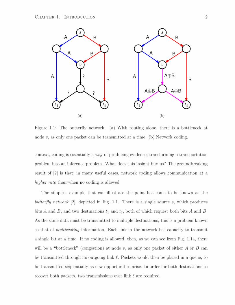
Figure 1.1: The butterfly network. (a) With routing alone, there is a bottleneck at
node v, as only one packet can be transmitted at a time. (b) Network coding.
context, coding is essentially a way of producing evidence, transforming a transportation
problem into an inference problem. What does this insight buy us? The groundbreaking
result of [2] is that, in many useful cases, network coding allows communication at a
higher rate than when no coding is allowed.
The simplest example that can illustrate the point has come to be known as the
butterfly network [2], depicted in Fig. 1.1. There is a single source s, which produces
bits A and B, and two destinations t1 and t2, both of which request both bits A and B.
As the same data must be transmitted to multiple destinations, this is a problem known
as that of multicasting information. Each link in the network has capacity to transmit
a single bit at a time. If no coding is allowed, then, as we can see from Fig. 1.1a, there
will be a “bottleneck” (congestion) at node v, as only one packet of either A or B can
be transmitted through its outgoing link ℓ. Packets would then be placed in a queue, to
be transmitted sequentially as new opportunities arise. In order for both destinations to
recover both packets, two transmissions over link ℓ are required.

Chapter 1. Introduction 3
On the other hand, if coding is allowed, then node v can simply transmit the XOR of
bits A and B, as illustrated in Fig. 1.1b. This allows destination t1 to recover B = A ⊕
(A⊕B) and destination t2 to recover A = B⊕ (A⊕B). Thus, by overcoming congestion,
network coding allows to increase the throughput of a communication network. More
precisely stated, to achieve the capacity of a multicast network in general, it is strictly
necessary to use network coding.
In contrast to the simple example of Fig. 1.1, real networks can be hugely complex.
If network coding is to be widely used, efficient coding (and decoding) operations must
be devised so that the benefits of network coding can be obtained without increasing the
implementation costs to a prohibitive level. In this context, two contributions can be
said to have raised network coding from a theoretical curiosity to a potential engineering
application: these are linear network coding [3,4] and random linear network coding [5,6].
With linear network coding, all coding operations at nodes are constrained to be linear
combinations of packets over a finite field. The importance of linear operations is that
they are arguably the simplest possible to perform in practice, and the fundamental
contribution of [3] is to show that no loss in multicast capacity is incurred if the field size is
sufficiently large. What exactly to choose as the coefficients of these linear combinations,
however, remains a problem. Must the network code be designed by a central authority
and informed individually to each node before transmission? The contribution of [6]
shows that a distributed design is sufficient in most cases. More precisely, if nodes choose
coefficients uniformly at random and independently from each other, then no capacity is
lost with high probability if the field size is sufficiently large. The actual coefficients used
can be easily recorded in the packet headers. As decoding corresponds to performing the
well-known algorithm of Gaussian elimination, random linear network coding becomes a
practical approach that can potentially be implemented over virtually any network.
An important benefit of random network coding is that, even in the cases where
network coding does not increase the throughput, it can greatly simplify the network

Chapter 1. Introduction 4
operation. The idea is that all “intelligence” is removed from the network (in the form
of scheduling and other algorithms) and is instead placed at its endpoints. The inter-
nal nodes are as “dumb” as possible, simply performing random linear combinations of
packets, with little regard to the conditions of farther nodes. One could argue that this
principle is consistent, for instance, with the design principle of the Internet [7], and
therefore represents an unavoidable trend.
Indeed, since its original publication in 2000, network coding has quickly emerged
into a major research area. The quickly growing list of contributions (see [8]) ranges
from theoretical inquiries on fundamental limits to real-world practical applications, and
provides sound evidence that network coding may indeed spur a revolution in network
communications in the near future.
1.2 Error Control
However elegant and compelling, the principle of network coding is not without its draw-
backs. Network coding achieves its benefits, essentially, by making every packet in the
network be statistically dependent on (almost) every other packet. However, this de-
pendence creates a problem. What if some of the packets are corrupted? As Fig. 1.2
illustrates, corrupt packets may contaminate other packets when coded at the internal
nodes, leading to an error propagation problem. Indeed, even a single corrupt packet
has the potential, when linearly combined with legitimate packets, to affect all packets
gathered by a destination node. This is in contrast to routing (no coding), where an
error in one packet affects only one source-destination path.
Thus, the phenomenon of error propagation in network coding can overwhelm the
error correction capability of any classical error-correcting code used to protect the data
end-to-end. The word “classical” here means designed for the Hamming metric. In short,
we might say that the Hamming metric is not well-suited to the end-to-end channel

Chapter 1. Introduction 5
.
.
.
.
.
.
s t
i
Figure 1.2: The phenomenon of error propagation induced by network coding. An error
occurred at the link i, which then propagated to the rightmost links after packet mixing.
induced by network coding. Thus, novel coding techniques are needed to solve this new
error correction problem. As we shall see, network coding requires error-correcting codes
designed for a different metric.
At this point, one might wonder whether considering this problem is indeed realistic.
Aren’t corrupt packets detected and immediately rejected by the lower network layers—
leading to an erasure rather than an undetected error? First, it must be noticed that the
physical-layer code may not always be perfect. Very reliable physical-layer codes require
very long block lengths, and there are several situations where a very short block length
is required for practical reasons (e.g., [9]). Thus, we must be able to cope with eventual
packet errors, without having to drop (and request retransmission of) all the received
packets.
Another compelling source of errors might be the presence of an adversary, i.e., a
user who does not comply with the protocol. Since the adversary injects corrupt packets
at the application layer, his effects cannot possibly be detected at the physical layer.
Adversarial errors represent an even more severe threat than random errors, since they
can be specifically designed to defeat the end-to-end error-correcting code.
Research into error-correcting codes for network coding started with [10–14], which

Chapter 1. Introduction 6
investigated fundamental limits for adversarial error correction under a deterministic (i.e.,
non-random) network coding setting. Code constructions for random network coding
were later proposed in [15, 16]; these constructions rely on using arbitrarily large packet
length and field size. In contrast, the framework proposed in [17,18] is valid for any field
or packet size. It can be said that their main philosophical contribution is to “take the
network out of the problem:” given any parameters of a random network coding system,
an end-to-end error-correcting scheme can be constructed providing any specified error-
correcting capability. Thus, the whole network can be seen simply as a (different kind
of) channel—in fact, a noncoherent multiple-input multiple-output finite field channel.
The work in [18] has been the main motivation for this thesis. Some of the questions
left open in [18], and which we tackle in this thesis, are the following. What are the
fundamental limits of this end-to-end approach? Can the approach be extended to the
deterministic setting of [11, 12]? And how can we design codes that simultaneously
exhibit good performance and yet admit computationally efficient encoding and decoding
algorithms? As we shall see, designing such efficient encoders and decoders is a vast
research problem on its own.
1.3 Information-Theoretic Security
Another issue brought up by the use of network coding lies in the field of information-
theoretic security. The issue has to do with the fact that the linear scrambling of packets
induced by network coding may actually be helpful to an eventual eavesdropper.
Consider the problem of securely transmitting a message over a network subject to
the presence of a wiretapper. More precisely, assume that the network supports the
reliable transmission of n packets from source to destination, and that the wiretapper
can intercept only µ < n packets (anywhere in the network). Suppose that the network
uses routing only. This problem is an instance of the wiretap channel II of Ozarow and
Chapter 1. Introduction 7
Wyner [19]. It can be shown that the maximum rate that can be achieved, such that
the wiretapper obtains no information about the message, is precisely n − µ packets
per network use. Moreover, a simple coding scheme achieving this rate can be obtained
as follows. First, generate µ packets uniformly at random; then, apply a (carefully
designed) invertible linear transformation to the collection of these µ random packets
together with the n − µ message packets, in order to produce the n packets that should
be transmitted. While the destination can easily invert the linear transformation and
obtain the message, the fact that “noise” was added to the transmission has the effect
of completely confusing the wiretapper. This happens because the linear transformation
has been carefully designed to produce a perfect mixing of message and noise.
Now, consider the case where the network uses linear network coding. It may be
the case that the linear scrambling performed by network coding actually “unscrambles”
part of the linear transformation applied at the source. In other words, network coding
may disrupt the perfect mixing of message and noise, and help the wiretapper obtain
non-negligible information about the message. Thus, network coding may significantly
impair the use of information-theoretic security.
In order to reconcile network coding and information-theoretic security, several works
have proposed a joint design of the network code and the outer linear transformation.
In [20, 21], security was achieved by carefully designing the linear transformation taking
into account a given network coding. In contrast, [22] proposed to design the network
code based on a specific linear transformation (one suitable for the routing-only problem).
A difficulty in all of these works is that they require a significantly large field size in order
for such a joint design to be possible. In other words, it is not possible under any of these
approaches to guarantee perfect information-theoretic security for a large network that
uses a small field size. In this spirit of the end-to-end approach of [18], we may formulate
the following question: is it possible to design an encoding that is universally secure, i.e.,
regardless of the network code and the field size?

Chapter 1. Introduction 8
At a first glance, the problem of error-control coding and information-theoretic secu-
rity seem barely related. Our motivation for addressing the latter problem is that the
techniques we propose for error correction are actually very helpful to solve the security
problem. We shall see that end-to-end codes designed for adversarial error correction
turn out to be closely related to linear transformations that are universally secure. Not
only can universal security be achieved: it can be implemented in an efficiently manner
using techniques similar to those for error control coding.
A final question that is natural at this point: is it possible to simultaneously provide
error control and information-theoretic security in the same random linear network coding
system?
As we see in Chapter 8, an affirmative answer can be obtained by appropriately
concatenating (layering) our proposed error control and security schemes; in particular,
no joint design is required, but simply a common interface.
1.4 Contributions
This thesis aims at providing a theoretical but practically-oriented solution to the prob-
lems of error control and security in network coding. The solutions we propose are
neither unique nor optimal, but lie in an (arguably) compelling point of the “theoretical
performance” versus “practical feasibility” tradeoff.
Our results can be divided into three main areas: correction of adversarial errors;
correction of random errors; and security against a wiretapper.
Our results for random error correction are the easiest to explain. This is because a
linear network coding channel that admits a probabilistic model can be understood and
analyzed using principles from information theory. Given such a probabilistic model, we
can define notions of channel capacity and capacity-achieving codes, as well as examine
the tradeoff between performance and delay. Our results in this area are the following:

Chapter 1. Introduction 9
We compute upper and lower bounds on the capacity of the random linear network
coding channel under a probabilistic error model. These bounds match (giving the
channel capacity) when either the field size or the packet length are large.
We present a simple coding scheme that asymptotically achieves the channel ca-
pacity when either the field size or the packet length grows.
For finite channel parameters, our coding scheme has simultaneously a better per-
formance and lower complexity than previous schemes [23].
We present extensions of our results for several variations of the channel.
In contrast to information theory, a unified framework is unavailable for treating
adversarial channels. The kind of adversarial channel discussed in this thesis (where the
adversary can inject at most t error packets) is most closely analogous to a binary vector
channel where an adversary may arbitrarily flip at most t bits—a channel for which
classical coding theory provides a complete and elegant solution. However, classical
coding theory alone is not enough to provide guidance for network error correction.
For instance, classical coding theory often requires a distance metric relating channel
input and output words; however, for the network coding channel, the input and output
alphabets may not even be the same (thus making it impossible to define any such
metric).
To fill this gap, we propose a coding theory for adversarial channels that is suitable
for the channels at hand. Such a theory is then specialized to coherent and noncoherent
network coding—the distinction is in whether or not the receiver has information about
the channel state. As in classical coding theory, the core notion of our theory is a
“distance function” that precisely describes the error correction capability of a code. The
close relationship between such distance functions (for both coherent and noncoherent
network coding) and the rank metric allows us to construct optimal or near-optimal
codes based on rank-metric codes. Moreover, decoding of our codes is shown to be

Chapter 1. Introduction 10
closely related to the decoding of rank-metric codes.
Our results for adversarial error correction comprise the main part of this thesis and
can be summarized as follows:
We define the concept of ∆-distance and compute this distance for both coherent
and noncoherent network coding. We then prove an “if and only if” statement
relating the minimum ∆-distance of a code and its error correction capability. A
consequence of this result is that—just as with classical coding theory—one can
ignore the channel model and focus solely on the combinatorial problem of finding
the largest code with a given minimum ∆-distance.
We show that a class of rank-metric codes called maximum-rank-distance (MRD)
codes are optimal for coherent network coding and can be slightly modified to
provide near-optimal codes for noncoherent network coding.
We show that the decoding problems for both coherent and noncoherent network
coding are mathematically equivalent and can be reformulated as a generalized
decoding problem for rank-metric codes.
We propose two algorithms for generalized rank-metric decoding: one is based on a
well-known “time-domain” algorithm and the other is based on a novel transform-
domain approach. We also propose two encoding algorithms, one for high-rate
systematic codes and another for nonsystematic codes.
The encoding and decoding algorithms we propose make use of optimal (or low-
complexity) normal bases to improve their speed. We show that these algorithms
are faster than any previous algorithms.
With respect to information-theoretic security, our framework follows closely that
of [22] (which in turn follows [19]). The novelty lies in the fact that we investigate more
general transformations to be applied at the source. More precisely, we show how one
can exploit the properties of rank-metric codes to achieve universal security. This is all

Chapter 1. Introduction 11
developed in the succinct and elegant algebraic language of finite field extensions, which
proves useful to investigate variations and generalizations of the problem. Our results in
this area are as follows:
We propose a MRD-based coding scheme that can provide universal security. We
show that the scheme is optimal in the sense of requiring the smallest packet length
possible for universal security.
We investigate the notion of weak security proposed in [24], as well as extensions
and variations of the problem, and show that universal weak security amounts to
the existence of matrices with certain properties. We then show that such matrices
always exist if the packet length (not the field size) is sufficiently large. In some
special cases we present coding schemes that are optimal in terms of packet length.
We address the case where wiretapper is also a jammer (who can introduce error
packets) and show that universal strong/weak security and error control can be
simultaneously achieved using a simple tandem scheme based on MRD codes.
The results in this thesis originated the following publications: [25–30] for adversarial
error correction, [31,32] for random error correction, and [33–35] for information-theoretic
security.
1.5 Outline
The remainder of the thesis is organized as follows. Chapter 2 reviews mathematical
preliminaries on linear algebra and finite field theory, as well as the theory of rank-metric
codes. Chapter 3 presents the basic model of a linear network coding channel subject to
errors. Chapters 4, 5 and 6 treat adversarial error correction, Chapter 7 treats random
error correction, and Chapter 8 treats information-theoretic security. Chapter 9 provides
our conclusions and suggestions for future work.

Chapter 1. Introduction 12
Due to the variety of subjects covered, we anticipate that this thesis may be read
by readers with distinct interests and backgrounds. To their benefit, this thesis can be
read in a modular fashion after Chapters 2 and 3. Readers who are interested only in
fundamental limits (i.e., capacity results) for network coding may read only Chapters 4,
7 and 8. Readers who are interested only in results for rank-metric codes may read only
Chapter 6 (possibly also Section 5.2). Readers who are only interested in error control
aspects of network coding may read Chapters 4, 5, 6 and 7 and skip Chapter 8, while
readers who are only interested in security issues may read only Chapter 8.

Chapter 2
Preliminaries
This chapter reviews necessary mathematical background and establishes the notation
used in this thesis. Sections 2.1 and 2.2 review linear algebra and finite-field algebra.
Section 2.3 reviews the basic theory of rank-metric codes. Section 2.4 reviews linearized
polynomials, which are used in Chapter 6 in the decoding of rank-metric codes. Sec-
tion 2.5 discusses the complexity of operations in normal bases; this section may safely
be skipped by readers who are not interested in implementation details.
We start with some miscellaneous notation. Let N = 0, 1, 2, . . .. Define [x]+ =
maxx, 0. Let 1[P ] represent the Iverson notation for a proposition P , i.e., 1[P ] is equal
to 1 if P is true and is equal to 0 otherwise.
2.1 Matrices and Subspaces
Let q ≥ 2 be a power of a prime, and let Fq denote the finite field with q elements. Let
Fn×mq denote the set of all n × m matrices over Fq, and set Fn
q = Fn×1q . In particular,
v ∈ Fnq is a column vector and v ∈ F1×m
q is a row vector.
If v is a vector, then the symbol vi denotes the ith entry of v. If A is a matrix, then
the symbol Ai may denote either the ith row or the ith column of A; the distinction will
always be clear from the way in which A is defined. In either case, the symbol Aij always
13

Chapter 2. Preliminaries 14
refers to the entry in the ith row and jth column of A.
For clarity, the n × m all-zero matrix and the n × n identity matrix are denoted by
0n×m and In×n, respectively, where the subscripts may be omitted when there is no risk of
confusion. If I = In×n, then our convention is that Ii denotes the ith column of I. More
generally, if U ⊆ 1, . . . , n, then IU = [Ii, i ∈ U ] denotes the sub-matrix of I consisting
of the columns indexed by U .
The row (column) rank of a matrix A ∈ Fn×mq is the maximum number of rows
(columns) of A that are linearly independent. The row rank and the column rank are
always equal and are simply called the rank of A, denoted by rank A. If rank A = n
(rank A = m), then A is said to have full row rank (column rank); otherwise, it is said
to have a row-rank (column-rank) deficiency of n− rank A (m− rank A). The maximum
possible rank for A is minn, m, in which case A is said to be a full-rank matrix.
Let wt(X) denote the number of nonzero rows of a matrix X. Clearly, rank X ≤
wt(X).
Let Tn×m,t(Fq) denote the set of all n × m matrices of rank t over Fq. We shall write
simply Tn×m,t = Tn×m,t(Fq) when the field Fq is clear from the context. We also use the
notation Tn×m = Tn×m,minn,m for the set of all full-rank n × m matrices.
The rank of a matrix X ∈ Fn×mq is the smallest r for which there exist matrices
P ∈ Fn×rq and Q ∈ Fr×m
q such that X = PQ, i.e.,
rank X = minr∈N,P∈F
n×rq ,Q∈F
r×mq :
X=PQ
r. (2.1)
Note that both matrices obtained in the decomposition are full-rank; accordingly, such
a decomposition is called a full-rank decomposition [36]. In this case, note that, by
partitioning P and Q, the matrix X can be further expanded as
M = PQ =
[
P ′ P ′′]
Q′
Q′′
= P ′Q′ + P ′′Q′′

Chapter 2. Preliminaries 15
where rank(P ′Q′)+ rank(P ′′Q′′) = r. In particular, X can be expanded as a sum of outer
products
X = PQ =
[
P1 · · · Pr
]
Q1
...
Qr
=
r∑
i=1
PiQi
where P1, . . . , Pr ∈ Fn×1q and Q1, . . . , Qr ∈ F1×m
q .
Two other useful properties of the rank function are given below [36]: for any X, Y ∈
Fn×mq , we have
rank(X + Y ) ≤ rank X + rank Y (2.4)
and, for X ∈ Fn×mq and A ∈ FN×n
q , we have
rank A + rank X − n ≤ rank AX ≤ minrank A, rank X. (2.5)
Let dim V denote the dimension of a vector space V. Let 〈v1, . . . , vk〉 denote the linear
span of a set of vectors v1, . . . , vk, and let 〈X〉 denote the row space of a matrix X. Recall
that F1×mq (or Fm
q ) is an m-dimensional vector space over Fq. The row space of X ∈ Fn×mq
is a subspace of F1×mq . Moreover, dim 〈X〉 = rank X.
Let U and V be subspaces of some fixed vector space. Recall that the sum
U + V = u + v : u ∈ U , v ∈ V
is the smallest vector space that contains both U and V. The intersection U ∩ V is the
largest vector space that is contained in both U and V. Recall also that
dim(U + V) = dim U + dim V − dim(U ∩ V). (2.7)
If X ∈ Fn×mq and Y ∈ FN×m
q are matrices, then a very useful fact about their row
spaces is that⟨
X
Y
⟩
= 〈X〉 + 〈Y 〉 . (2.8)

Chapter 2. Preliminaries 16
Therefore,
rank
X
Y
= dim(〈X〉 + 〈Y 〉)
= rank X + rank Y − dim(〈X〉 ∩ 〈Y 〉). (2.9)
Let P(Fmq ) denote the set of all subspaces of Fm
q . Assume n ≤ m. The Grassmannian
Pn(Fmq ) is the set of all n-dimensional subspaces of Fm
q . Define
Pmaxn (Fm
q ) =
n⋃
k=0
Pk(Fmq )
as the set of all subspaces of Fmq with dimension up to n. Let RRE (X) denote the
reduced row echelon (RRE) form of a matrix X. Note that there exists a bijection
between Pmaxn (Fm
q ) and the subset of Fn×mq consisting of matrices in RRE form. In other
words, every subspace V ∈ Pmaxn (Fm
q ) can be uniquely represented by a matrix X ∈ Fn×mq
in RRE form such that V = 〈X〉. In particular, every subspace in Pn(Fmq ) is associated
with a matrix in Tn×m in RRE form.
The size of the Grassmannian Pn(Fmq ) is given by the Gaussian coefficient
[m
n
]
q
=n−1∏
i=0
(qm − qi)
(qn − qi).
Two useful properties of the Gaussian coefficient are [18, Lemma 5]
qn(m−n) <
[m
n
]
q
< 4qn(m−n) (2.12)
and [37][m
n
]
q
[n
t
]
q
=
[m
t
]
q
[m − t
n − t
]
q
, t ≤ n ≤ m. (2.13)
The Gaussian coefficient also arises when computing the size of Tn×m,t. It can be

Chapter 2. Preliminaries 17
shown that the number of n × m matrices of rank t is given by [38, p. 455]
|Tn×m,t| =|Tn×t||Tt×m|
|Tt×t|= |Tn×t|
[m
t
]
q
(2.14)
= q(n+m−t)t
t−1∏
i=0
(1 − qi−n)(1 − qi−m)
(1 − qi−t). (2.15)
A method of computing the RRE form of a matrix is the well-known Gaussian (or
rather, Gauss-Jordan) elimination [39]. It is a straightforward exercise to show that
the number of operations needed to convert an n × m matrix of rank r to RRE form
(assuming n ≤ m) is no more that r divisions, 12rn(2m − r − 1) multiplications, and
12r(n − 1)(2m − r − 1) additions in Fq.
2.2 Bases over Finite Fields
For convenience, when dealing with bases over finite fields, we assume that the entries of
all bases, vectors and matrices are indexed starting from 0.
Let V be n-dimensional vector space over Fq with an ordered basis A = α0, . . . , αn−1.
For v ∈ V, we denote by
[
v
]
A
the coordinate vector of v relative to A; that is,[
v
]
A
=
[
v0 · · · vn−1
]
, where v0, . . . , vn−1 are the unique elements in Fq such that
v =∑n−1
i=0 viαi. When the basis A is clear from context, we shall use the simplified
notation v ,
[
v
]
A
.
Let W be an m-dimensional vector space over Fq with ordered basis B = β0, . . . , βm−1,
and let T be a linear transformation from V to W. We denote by
[
T
]B
A
the matrix rep-
resentation of T in the bases A and B; that is,
[
T
]B
A
is the unique n×m matrix over Fq
such that
T (αi) =m−1∑
j=0
([
T
]B
A
)
ij
βj , i = 0, . . . , n − 1. (2.16)

Chapter 2. Preliminaries 18
With these notations, we have, for v ∈ V,
[
T (v)
]
B
=
[
v
]
A
[
T
]B
A
.
Let U be a k-dimensional vector space over Fq with ordered basis Θ = θ0, . . . , θk−1,
and let S be a linear transformation from W to U . Recall that [39]
[
S T
]Θ
A
=
[
T
]B
A
[
S
]Θ
B
. (2.18)
Let Fqm be an extension field of Fq. Recall that every extension field can be regarded
as a vector space over the base field. Let A = α0, . . . , αm−1 be a basis for Fqm over Fq.
If A is of the form A = α0, α1, . . . , αm−1, then A is called a polynomial (or standard)
basis. If A is of the form A =
αq0, αq1
, . . . , αqm−1
, then A is called a normal basis, and
α is called a normal element [38].
Every basis over a finite field admits a dual basis. The dual basis of A is the unique
basis A′ = α′0, . . . , α′m−1 such that
Tr(αiα′j) =
1 i = j
0 otherwise
where Tr(β) =∑m−1
k=0 βqk
denotes the trace of an element β ∈ Fqm [38]. Note that β 7→ βq
is an Fq-linear operator. It follows that if [β]A =
[
β0 · · · βn−1
]
, then βj = Tr(βα′j), for
all j. An important property of the trace is that it always returns elements in the base
field, i.e., Tr(β) ∈ Fq, for all β ∈ Fqm . Moreover,
Tr(βq) = Tr(β), for all β ∈ Fqm (2.20)
due to the fact that βqm
= β in Fqm.
A basis is self-dual if it is equal (in the same order) to its dual basis.
Chapter 2. Preliminaries 19
2.3 Rank-Metric Codes
Let X, Y ∈ Fn×mq be matrices. The rank distance between X and Y is defined as
dR(X, Y ) , rank(Y − X).
As observed in [37, 40], the rank distance is indeed a metric. In particular, the triangle
inequality follows directly from (2.4). Thus, Fn×mq is a metric space.
A rank-metric code C ⊆ Fn×mq is a matrix code (i.e., a nonempty set of matrices) used
in the context of the rank metric. The minimum rank distance of C, denoted dR(C), is
the minimum rank distance between all pairs of distinct codewords of C.
Rank-metric codes are typically used as error-correcting codes. A minimum distance
decoder for a rank-metric code C ⊆ Fn×mq takes a word r ∈ Fn×m
q and returns a codeword
x ∈ C that is closest to r in rank distance, that is,
x = argminx∈C
rank(r − x). (2.22)
Note that if dR(x, r) < dR(C)/2, then a minimum distance decoder is guaranteed to return
x = x. Throughout this text, we refer to problem (2.22) as the conventional rank-metric
decoding problem.
There is a rich coding theory for rank-metric codes that is analogous to the classical
coding theory in the Hamming metric. In particular, the Singleton bound for the rank
metric [37, 41] (see also [27, 42, 43]) states that every rank-metric code C ⊆ Fn×mq with
minimum rank distance d must satisfy
|C| ≤ qmaxn,m(minn,m−d+1). (2.23)
Codes that achieve this bound are called maximum-rank-distance (MRD) codes and they
are known to exist for all choices of parameters q, n, m and d ≤ minn, m [37].
In order to construct rank-metric codes, it is useful to endow Fn×mq with additional
algebraic properties. Specifically, it is useful to regard F1×mq as the finite field Fqm (i.e.,
Chapter 2. Preliminaries 20
endowing it with a multiplication operation). More precisely, let A be a basis for Fqm over
Fq. Then we can extend the bijection [·]A : Fqm → F1×mq to a bijection [·]A : Fn
qm → Fn×mq
given by
[
x
]
A
=
[
x0
]
A...
[
xn−1
]
A
where x ∈ Fnqm . As before, we shall use the simplified notation x ,
[
x
]
A
when A is fixed.
Note that x ∈ Fnqm is a length-n (column) vector over the field Fqm , while x is an n × m
matrix over Fq. Thus, concepts such as the rank of a vector x ∈ Fnqm or the rank distance
between vectors x, y ∈ Fnqm are naturally defined through their matrix counterparts. In
this context, a rank-metric code C ⊆ Fnqm is simply a block code of length n over Fqm .
(Note that, differently from classical coding theory, here we treat each codeword as a
column vector.)
It is particularly useful to consider linear block codes over Fqm . For linear (n, k) codes
over Fqm with minimum rank distance d, the Singleton bound becomes
d ≤ min
1,m
n
(n − k) + 1. (2.25)
Note that the classical Singleton bound d ≤ n − k + 1 can be achieved only if m ≥ n;
that is, a code has d = n − k + 1 if and only if it is MRD and m ≥ n. The similarity
with the classical Singleton bound is not accidental: every MRD code with m ≥ n is also
MDS as a block code over Fqm.
Such a class of linear MRD codes can be characterized by the following theorem [37].
Theorem 2.1: Let C be a linear (n, k) code over Fqm with parity-check matrix H ∈
F(n−k)×nqm . Then C is an MRD code with m ≥ n if and only if the matrix HT is nonsingular
for any full-rank matrix T ∈ Fn×(n−k)q .
For m ≥ n, an important class of rank-metric codes was proposed by Gabidulin [37].
For convenience, let [i] denote qi. A Gabidulin code is a linear (n, k) code over Fqm defined

Chapter 2. Preliminaries 21
by the parity-check matrix
H =
h[0]0 h
[0]1 · · · h
[0]n−1
h[1]0 h
[1]1 · · · h
[1]n−1
......
. . ....
h[n−k−1]0 h
[n−k−1]1 · · · h
[n−k−1]n−1
(2.26)
where the elements h0, . . . , hn−1 ∈ Fqm are linearly independent over Fq. It can be shown
that the minimum rank distance of a Gabidulin code is d = n − k + 1, so it is an MRD
code [37]. Encoding and decoding of Gabidulin codes can be performed efficiently; this
topic is covered in more detail in Chapter 6.
Besides the matrix version and the block version, yet a third (and most general)
definition of rank-metric codes is possible. This definition arises when we take the code
“alphabet” to be, rather than F1×mq or Fqm , a general vector space V with dimension m
over Fq.
Consider the set Vn of n-tuples with components from V. Recall, once again, that
we may establish a bijection between Vn and Fn×mq once a basis is fixed for V over Fq.
Under this bijection, the rank of a tuple x ∈ Vn can be defined as the rank of the
corresponding matrix, and similarly for the rank distance. This turns Vn into a metric
space. A rank-metric code is simply a subset of Vn.
This abstract definition is particularly useful when V is also a vector space over a
larger field, say, over Fqℓ . In this situation, we may explicitly refer to a rank-metric
code over V/Fq, in order to emphasize the field Fq with respect to which a bijection
is established. Note that this definition encompasses the previous two, as we can take
V = F1×mq or V = Fqm .
For convenience, define a “matrix-by-tuple” multiplication in the natural way: for
A = [Aij ] ∈ Fk×nq and x = [xi] ∈ Vn, denote by Ax the tuple y = [yi] ∈ Vk given by
yi =∑n−1
j=0 Aijxj, i = 0, . . . , k − 1.
Note that, when m ≥ n, the Singleton bound (2.25) exhibits no dependency on m.

Chapter 2. Preliminaries 22
Thus, if n|m, any linear (n, k) MRD code over Fqn/Fq can be used to construct an MRD
code over V/Fq, as shown in the following theorem.
Theorem 2.2: Let V be a vector space over Fqn . Let C1 be a linear (n, k) MRD code over
Fqn with generator and parity-check matrices G ∈ Fk×nqn and H ∈ F
(n−k)×nqn , respectively.
Then C ⊆ Vn defined by
C = GTU, U ∈ Vk = X ∈ Vn : HX = 0
is an MRD code over V/Fq.
Proof: Let r be the dimension of V as a vector space over Fqn. Then C is isomorphic to
an r-fold Cartesian product of C1 with itself and thus dR(C) = dR(C1).
From a matrix perspective (i.e., by expanding V as a vector space over Fqn), the code C
in Theorem 2.2 is the set of all n × r matrices over Fqn obtained by “gluing together”
any r = m/n codewords of C1.
2.4 Linearized Polynomials
Linear transformations from Fqm to itself can be elegantly described in terms of linearized
polynomials. A linearized polynomial or q-polynomial over Fqm [38] is a polynomial of
the form
f(x) =
n∑
i=0
fix[i]
where fi ∈ Fqm. If fn 6= 0, we call n the q-degree of f(x). It is easy to see that evaluation
of a linearized polynomial is indeed an Fq-linear transformation from Fqm to itself. In
particular, the set of roots in Fqm of a linearized polynomial is the kernel of the associated
map (and therefore a subspace of Fqm).

Chapter 2. Preliminaries 23
It is well-known that the set of linearized polynomials over Fqm forms a noncommu-
tative ring (actually, an algebra over Fq) under addition and composition (evaluation).
The latter operation is usually called symbolic multiplication in this context and denoted
by f(x) ⊗ g(x) = f(g(x)). Note that if n and k are the q-degrees of f(x) and g(x),
respectively, then P (x) = f(x) ⊗ g(x) has q-degree equal to t = n + k. Moreover, the
coefficients of P (x) can be computed as
Pℓ =
minℓ,n∑
i=max0,ℓ−k
fig[i]ℓ−i =
minℓ,k∑
j=max0,ℓ−n
fℓ−jg[ℓ−j]j , ℓ = 0, . . . , t.
In particular, if n ≤ k, then
Pℓ =
n∑
i=0
fig[i]ℓ−i, n ≤ ℓ ≤ k (2.30)
while if k ≤ n, then
Pℓ =
k∑
j=0
fℓ−jg[ℓ−j]j , k ≤ ℓ ≤ n. (2.31)
One of the most convenient properties of linearized polynomials is to provide canonical
maps for specified kernels. There is a unique linearized polynomial MS(x) =∑t
i=0 Mix[i]
with smallest q-degree and M0 = 1 whose root space contains a specified set S ⊆ Fqm .
This polynomial is called the minimal q-polynomial of S. The q-degree of MS(x) is
precisely equal to the dimension of the space spanned by S, and is also equal to the
nullity of MS(x) as a linear map. The polynomial MS(x) can be computed recursively.
Let s1, . . . , st be a basis for the space spanned by S. Then we can find MS(x) by
computing Ms1(x) = x − x[1]s1/s[1]1 and, for i = 2, . . . , t, zi = Ms1,...,si−1(si) and
Ms1,...,si(x) = Mzi(x) ⊗ Ms1,...,si−1(x).
It is useful to define two notions of reverse linearized polynomials. In the first def-
inition, we are given a linearized polynomial f(x) =∑t
i=0 fix[i] whose q-degree does
not exceed a specified number t. Then the partial q-reverse of f(x) is the polynomial
f(x) =∑t
i=0 fix[i] given by fi = f
[i−t]t−i , for i = 0, . . . , t. If t is not specified, it is taken
as the q-degree of f(x). In the second definition, we are given a linearized polynomial

Chapter 2. Preliminaries 24
Table 2.1: Complexity of operations with linearized polynomials. See text for details.
OperationNumber of operations in Fqm
Multiplications Additions q-Exponentiations Inversions
f(x) ⊗ g(x) n′k′ nk nk′ –
f(β) n′ n n –
S 7→ MS(x) t2 t(t − 1) t2 t
f(x) =∑m−1
i=0 fix[i] of q-degree at most m − 1. Then the full q-reverse of f(x) is the
polynomial f(x) =∑m−1
i=0 fix[i] given by fi = f
[i]−i mod m, i = 0, . . . , m− 1. Note that a full
q-reverse can be seen as a partial q-reverse with t = m and indices taken modulo m. As
we will see in Chapter 6, a full q-reverse is closely related to the transpose of a matrix
representing a linear map.
It is worth mentioning that Gabidulin codes can be described in terms of linearized
polynomials, just as Reed-Solomon codes can be described in terms of conventional poly-
nomials. It is shown in [37] that the generator matrix of a Gabidulin code is of the
form
G =
g[0]0 g
[0]1 · · · g
[0]n−1
g[1]0 g
[1]1 · · · g
[1]n−1
......
. . ....
g[k−1]0 g
[k−1]1 · · · g
[k−1]n−1
for some linearly independent g0, . . . , gn−1 ∈ Fqm. Thus, a Gabidulin code may be de-
scribed as the set of all codewords c ∈ Fnqm such that ci = f(gi), i = 0, . . . , n − 1, for
some linearized polynomial f(x) of q-degree at most k − 1.
Table 2.1 lists the complexity of some useful operations with linearized polynomials.
In the table, β is any element of Fqm , t denotes the size of S ⊆ Fqm, and f(x) and g(x)
are linearized polynomials with q-degrees n and k, respectively. Additionally, n′ = n if

Chapter 2. Preliminaries 25
f(x) is monic and n′ = n + 1 otherwise; similarly, k′ = k if g(x) is monic and k′ = k + 1
otherwise.
2.5 Operations in Normal Bases
Let α ∈ Fqm be a normal element, and fix a basis A =α[0], . . . , α[m−1]
. In a practical
implementation, an element a ∈ Fqm is usually represented as the vector a over the base
field Fq. It is useful to review the complexity of some common operations in Fqm when
elements are represented in this form. For convenience, let JαK denote the column vector[
α[0] · · · α[m−1]
]T
. Then any element a ∈ Fqm can be written as a = a JαK.
For a vector a =
[
a0, . . . , am−1
]
∈ F1×mq , let a←i denote a cyclic shift to the left by i
positions, that is, a←i =
[
ai, . . . , am−1, a0, . . . , ai−1
]
. Similarly, let a→i = a←m−i. In this
notation, we have a[i] = a→i JαK, or a[i] = a→i. Thus, q-exponentiation in a normal basis
corresponds to a cyclic shift.
Multiplications in normal bases are usually performed in the following way. Let
T = [Tij] ∈ Fn×mq be a matrix such that αα[i] =
∑m−1j=0 Tijα
[j], i = 0, . . . , m − 1. The
matrix T is called the multiplication table of the normal basis. The number of nonzero
entries in T is denoted by C(T ) and is called the complexity of the normal basis [44].
Note that α JαK = T JαK. It can be shown that, if a, b ∈ Fqm , then
ab =m−1∑
i=0
bi
(a←iT
)→i.
Thus, a general multiplication in a normal basis requires mC(T ) + m2 multiplications
and mC(T ) − 1 additions in Fq. Clearly, this is only efficient if T is sparse; otherwise,
it is more advantageous to convert back and forth to a polynomial basis to perform
multiplication.
It is a well-known result that the complexity of a normal basis is lower bounded by
2m − 1. Bases that achieve this complexity are called optimal. More generally, low-

Chapter 2. Preliminaries 26
Table 2.2: Complexity of operations in Fqm using a normal basis constructed via Gauss
periods, for q a power of 2.
Operation in Fqm
Number of operations in Fq
Multiplications Additions Inversions
Multiplication m2 m(C(T ) − 1) –
Addition – m –
Inversion 52m2 + O(m) 4m2 + O(m) m + 2
complexity (but not necessarily optimal) normal bases can be constructed using Gauss
periods, as described in detail in [44]. For q = 2s, such a construction is possible if
and only if m satisfies gcd(m, s) = 1 and 8 ∤ m [45]. As an example, for q = 256, this
condition is satisfied for any odd m. Among the odd m ≤ 100, the normal bases that
result are in fact optimal when m = 3, 5, 9, 11, 23, 29, 33, 35, 39, 41, 51, 53, 65, 69,
81, 83, 89, 95, 99. For q = 2s and odd m, all of the normal bases constructed by Gauss
periods are self-dual [45].
An interesting fact about a normal basis constructed via Gauss periods is that its
multiplication table T lies entirely in the prime field Fp, where p is the characteristic
of q. This in turn implies that the minimal polynomial of α has coefficients in Fp and
the conversion matrices from/to the standard basis α0, α1, . . . , αm−1 have entries also
in Fp.
In this thesis, we are mostly interested in the case p = 2. In this case, multiplication
by T can be done simply by using XORs. In Table 2.2, we give the complexity of
each operation in Fqm assuming that p = 2. We also assume that q-exponentiations are
free. Note that inversion can be performed using the extended Euclidean algorithm on a
standard basis, which takes at most 52m2 + O(m) multiplications, 2m2 + O(m) additions
and m + 2 inversions in Fq [46]. Converting between standard and normal basis takes at

Chapter 2. Preliminaries 27
most m(m − 1) additions since the conversion matrices lie in F2.
Chapter 3
The Linear Network Coding
Channel
This chapter describes a channel model for communication over a network subject to
packet errors. This model is an extension of the linear network coding model, which is
reviewed in Section 3.1.
Network coding was proposed in [2] by Ahlswede, Cai, Li, and Yeung. Linear network
coding was proposed in [3] by Li et al., and later received an algebraic formulation by
Koetter and Medard [4]. The idea of random linear network coding was proposed by Ho et
al. [5, 6] and subsequently implemented by Chou et al. [47]. The additive matrix model
for network coding with errors, which we review in this chapter, was first mentioned
in [13] and [15], although it had been implicit from [4]. Subsequent work that is based
on this model includes [48] and [18].
3.1 Linear Network Coding
Consider a communication network represented by a directed multigraph with unit ca-
pacity edges. The network is used for single-source multicasting : there is a single source
node, which produces a message, and multiple destination nodes, all of which demand
28

Chapter 3. The Linear Network Coding Channel 29
the message. All the remaining nodes are called internal nodes. Each link in the network
is assumed to transport, free of errors, a packet (i.e., a vector) of m symbols from a finite
field Fq. A packet transmitted on a link directed from a node u to a node v is said to be
an outgoing packet of u and an incoming packet of v. The message to be transmitted by
the source node is a matrix X ∈ Fn×mq , where n is a positive integer. The n rows of this
matrix, denoted by X1, . . . , Xn ∈ F1×mq , are assumed to be the incoming packets of the
source node.
The network runs as follows: at each transmission opportunity, a node computes an
outgoing packet as an Fq-linear combination of incoming packets. It is easy to see that
a packet Pi transmitted on an edge i must be an Fq-linear combination of the source
packets, i.e., Pi = giX, where gi ∈ F1×nq . The vector gi is called the global coding vector
of edge i. Consider some specific destination node, and let Y ∈ FN×mq be a matrix whose
rows are the N packets received by this node. It follows that
Y = AX (3.1)
for some matrix A ∈ FN×nq , which is called the transfer matrix of the network (from the
source node to that destination node). It is clear that all destination nodes can obtain X
if (and only if, in the case that X is a uniform random variable) all the transfer matrices
have rank n, in which case the network code is said to be feasible.
It is important to mention that (3.1) holds under a variety of situations:
Any network topology is allowed (in particular, the network may contain cycles);
The network may be reused for multiple rounds (called generations in [47]), ex-
hibiting possibly different transfer matrices;
Packet transmissions may contain delays and the overall topology may be time-
varying;
Wireless broadcast transmissions may be modeled by constraining a node to send
the same packet on each of its outgoing links;

Chapter 3. The Linear Network Coding Channel 30
Erasure channels may be modeled by assuming that each link is the instantiation
of a successful packet transmission.
Let h be the minimum source-destination min-cut among all the destination nodes. In
a general network code (not necessarily linear), nodes are allowed to perform any arbitrary
operations on packets. It is shown in [2] that a feasible network code exists if and only
if n ≤ h and the packet size qm is sufficiently large. Assuming that n ≤ h, a remarkable
result of [3] (see also [4]) is that a feasible linear network code always exists if the field
size q is sufficiently large. If q is at least the number of destination nodes, such a code
can be constructed in polynomial time by a centralized algorithm [49]. Alternatively, the
network code can be constructed in a decentralized fashion by having nodes select coding
coefficients uniformly at random from Fq. As shown in [6], such a random network code is
feasible with high probability if q is sufficiently large. In order to inform the destination
nodes about the specific realization of the network code (or rather their corresponding
transfer matrices), a typical approach is to prepend to X an identity matrix [6, 47]. In
this way, each packet will contain a header that records its global coding vector as the
packet traverses the network.
For the remainder of this text, we assume for simplicity that there is a single desti-
nation node. For the problems considered here, each destination node will behave in a
similar manner, so any generalization to multicast is straightforward.
3.2 Linear Network Coding with Packet Errors
We now extend the model of the previous section to include the possibility of packet er-
rors. That model assumes that, for every link in the network, the following two conditions
are satisfied:
the link is an error-free channel;
the transmitter node at the link complies with the established protocol.
Chapter 3. The Linear Network Coding Channel 31
Ei
u vP
(ideal)i
P(rec)i
u vi
=⇒
Pi
+
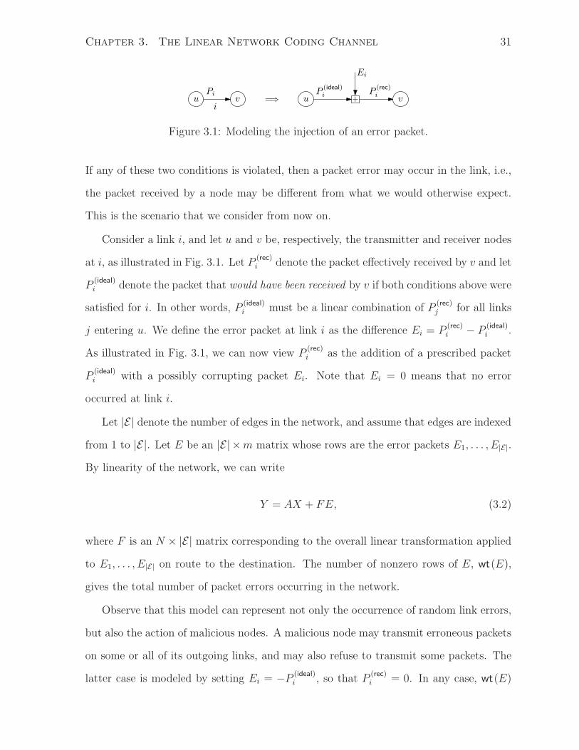
Figure 3.1: Modeling the injection of an error packet.
If any of these two conditions is violated, then a packet error may occur in the link, i.e.,
the packet received by a node may be different from what we would otherwise expect.
This is the scenario that we consider from now on.
Consider a link i, and let u and v be, respectively, the transmitter and receiver nodes
at i, as illustrated in Fig. 3.1. Let P(rec)i denote the packet effectively received by v and let
P(ideal)i denote the packet that would have been received by v if both conditions above were
satisfied for i. In other words, P(ideal)i must be a linear combination of P
(rec)j for all links
j entering u. We define the error packet at link i as the difference Ei = P(rec)i − P
(ideal)i .
As illustrated in Fig. 3.1, we can now view P(rec)i as the addition of a prescribed packet
P(ideal)i with a possibly corrupting packet Ei. Note that Ei = 0 means that no error
occurred at link i.
Let |E| denote the number of edges in the network, and assume that edges are indexed
from 1 to |E|. Let E be an |E| ×m matrix whose rows are the error packets E1, . . . , E|E|.
By linearity of the network, we can write
Y = AX + FE, (3.2)
where F is an N × |E| matrix corresponding to the overall linear transformation applied
to E1, . . . , E|E| on route to the destination. The number of nonzero rows of E, wt(E),
gives the total number of packet errors occurring in the network.
Observe that this model can represent not only the occurrence of random link errors,
but also the action of malicious nodes. A malicious node may transmit erroneous packets
on some or all of its outgoing links, and may also refuse to transmit some packets. The
latter case is modeled by setting Ei = −P(ideal)i , so that P
(rec)i = 0. In any case, wt(E)

Chapter 3. The Linear Network Coding Channel 32
gives the total number of “packet interventions” performed by all malicious nodes and
thus gives a sense of the total adversarial “effort” employed towards jamming the network.
Equation (3.2) is our basic model of an additive error channel induced by linear
network coding, and we will refer to it as the linear network coding channel (LNCC).
The channel input and output alphabets are given by Fn×mq and FN×m
q , respectively. The
conditional probability of Y given X is given by
Pr(Y |X) = Pr(A, F, E|X)1[Y = AX + FE].
Clearly, we still need to specify joint distribution of A, F and E given X in order to fully
specify the channel. For generality, we leave this open in the definition of the LNCC and
proceed below to discuss a number of special cases.
Definition 3.1: An LNCC is called coherent if the transfer matrix A is a constant known
to the receiver; otherwise it is called noncoherent.
The definition of coherent LNCC is motivated by a scenario where the network code is
designed by a central entity and informed to each node in the network before transmission
starts; in this case, the matrix F would naturally be known at the receiver. A noncoherent
LNCC, on the other hand, is motivated by the use of random network coding, in which
case both A and F would be random and unknown.1 Note that Definition 3.1 also applies
also to an LNCC free of errors (as in Section 3.1).
Definition 3.2: An LNCC is said to have a random or probabilistic error model if the
matrix E is a random variable independent from (A, F, X). Otherwise, the error model
is said to be adversarial.
1One might wonder if our definition is appropriate for the case where A is known only at the trans-mitter but not at the receiver. We believe that this situation is undeserving of a definition for thefollowing reasons: if the network code varies from time to time, then it is unlikely that the transmitter(and only the transmitter) would have knowledge of A; on the other hand, if the network code is fixed,then it should be a simple matter to communicate the transfer matrix to the receiver before messagetransmission (say, through a control channel as the receiver joins the system, or even by using a singleround of noncoherent network coding).

Chapter 3. The Linear Network Coding Channel 33
A random error model corresponds to dropping the assumption that the links are
error-free, while an adversarial error model corresponds to dropping the assumption that
the nodes comply with the protocol, i.e., some nodes may be malicious, as discussed
above.
A main assumption made throughout this thesis is that the number of error packets
injected in the network is limited, i.e., wt(E) ≤ t. This assumption allows us to rewrite
(3.2) as
Y = AX + DZ, (3.4)
where Z ∈ Ft×mq consists of the (potentially) nonzero rows of E, and D ∈ FN×t
q is a
submatrix of F . We use expression (3.4) for the most part of this thesis.
In the next three chapters, we address the problem of error correction for an LNCC
(either coherent or noncoherent) with an adversarial error model. An LNCC with a
probabilistic error model is investigated in Chapter 7.

Chapter 4
Error Control under an Adversarial
Error Model
This chapter addresses the problem of error control in linear network coding under an
adversarial error model. One main insight of our approach is that both the coherent and
the noncoherent LNCCs can be characterized by a parameter that we call maximum dis-
crepancy. In Section 4.1, we start by proposing a general theory for adversarial channels
that admit such characterization. The theory generalizes classical coding theory in that
it provides us with a function—the ∆-distance—that perfectly describes the correction
capability of a code. We use this approach in Sections 4.2 and 4.3 to study coherent and
noncoherent network coding, respectively.
Our results in Sections 4.2 and 4.3 are closely related to those of Yeung et al. [11,48]
and Kotter and Kschischang [18], respectively. Comparisons with such works are made
in the corresponding Sections 4.2.2 and 4.3.2. Our main result in Section 4.2 is to
show that, under certain mild conditions, MRD codes are optimal for the correction of
adversarial errors in coherent network coding. Section 4.3 contains two main results:
we provide a precise framework for assessing optimality of error-correcting codes for
noncoherent network coding (which was missing in [18]); and we show that a class of
34

Chapter 4. Error Control under an Adversarial Error Model 35
MRD-based codes—which we call liftings of MRD codes—are nearly optimal for any
practical purposes.
Finally, Section 4.4 discusses the decoding problems that arise in coherent network
coding, as well as in noncoherent network coding when the lifting approach is used, and
shows that these two problems are mathematically equivalent. The discussion opens
grounds for investigating efficient decoding algorithms, which is done in Chapter 5.
In this chapter we use the following notation. Let X be a set, and let C ⊆ X .
Whenever a function d : X × X → N is defined, denote
d(C) , minx,x′∈C: x 6=x′
d(x, x′).
If d(x, x′) is called a “distance” between x and x′, then d(C) is called the minimum
“distance” of C.
4.1 A General Approach
This section presents a general approach to error correction over adversarial channels.
This approach is specialized to coherent and noncoherent network coding in sections 4.2
and 4.3, respectively.
4.1.1 Adversarial Channels
An adversarial channel is specified by a finite input alphabet X , a finite output alphabet
Y and a collection of output sets Y(x) ⊆ Y for all x ∈ X . For each input x, the output
y is constrained to be in Y(x) but is otherwise arbitrarily chosen by an adversary. The
constraint on the output is important: otherwise, the adversary could prevent commu-
nication simply by mapping all inputs to the same output. No further restrictions are
imposed on the adversary; in particular, the adversary is potentially omniscient and has
unlimited computational power.

Chapter 4. Error Control under an Adversarial Error Model 36
A code for an adversarial channel is a subset1 C ⊆ X . We say that a code is unam-
biguous for a channel if the input codeword can always be uniquely determined from the
channel output. More precisely, a code C is unambiguous if the sets Y(x), x ∈ C, are
pairwise disjoint. The importance of this concept lies in the fact that, if the code is not
unambiguous, then there exist codewords x, x′ that are indistinguishable at the decoder:
if Y(x)∩Y(x′) 6= ∅, then the adversary can (and will) exploit this ambiguity by mapping
both x and x′ to the same output.
A decoder for a code C is any function x : Y → C ∪ f, where f 6∈ C denotes a
decoding failure (detected error). When x ∈ C is transmitted and y ∈ Y(x) is received,
a decoder is said to be successful if x(y) = x. We say that a decoder is infallible if it is
successful for all y ∈ Y(x) and all x ∈ C. Note that the existence of an infallible decoder
for C implies that C is unambiguous. Conversely, given any unambiguous code C, one can
always find (by definition) a decoder that is infallible. One example is the exhaustive
decoder
x(y) =
x if y ∈ Y(x) and y 6∈ Y(x′) for all x′ ∈ C, x′ = x
f otherwise.
In other words, an exhaustive decoder returns x if x is the unique codeword that could
possibly have been transmitted when y is received, and returns a failure otherwise.
Ideally, one would like to find a large (or largest) code that is unambiguous for a
given adversarial channel, together with a decoder that is infallible (and computationally-
efficient to implement).
1There is no loss of generality in considering a single channel use, since the channel may be taken tocorrespond to multiple uses of a simpler channel.

Chapter 4. Error Control under an Adversarial Error Model 37
4.1.2 Discrepancy
It is useful to consider adversarial channels parameterized by an adversarial effort t ∈ N.
Assume that the output sets are of the form
Y(x) = y ∈ Y : ∆(x, y) ≤ t (4.3)
for some ∆: X×Y → N. The value ∆(x, y), which we call the discrepancy between x and
y, represents the minimum effort needed for an adversary to transform an input x into
an output y. The value of t then represents the maximum adversarial effort (maximum
discrepancy) allowed in the channel.
In principle, there is no loss of generality in assuming (4.3) since, by properly defining
∆(x, y), one can always express any Y(x) in this form. For instance, one could set
∆(x, y) = 0 if y ∈ Y(x), and ∆(x, y) = ∞ otherwise. However, such a definition
would be of no practical value since ∆(x, y) would be merely an indicator function.
Thus, an effective limitation of our model is that it requires channels that are naturally
characterized by some discrepancy function. In particular, one should be able to interpret
the maximum discrepancy t as the level of “degradedness” of the channel.
On the other hand, the assumption ∆(x, y) ∈ N imposes effectively no constraint.
Since |X × Y| is finite, given any “naturally defined” ∆′ : X × Y → R, one can always
shift, scale and round the image of ∆′ in order to produce some ∆: X × Y → N that
induces the same output sets as ∆′ for all t.
Example 4.1: Let us use the above notation to define a t-error channel, i.e., a vector
channel that introduces at most t symbol errors (arbitrarily chosen by an adversary).
Assume that the channel input and output alphabets are given by X = Y = Fnq . It is
easy to see that the channel can be characterized by a discrepancy function that counts
the number of components in which an input vector x and an output vector y differ.
More precisely, we have ∆(x, y) = dH(x, y), where dH(·, ·) denotes the Hamming distance
function.

Chapter 4. Error Control under an Adversarial Error Model 38
A main feature of our proposed discrepancy characterization is to allow us to study a
whole family of channels (with various levels of degradedness) under the same framework.
For instance, we can use a single decoder for all channels in the same family. Define the
minimum-discrepancy decoder given by
x = argminx∈C
∆(x, y) (4.4)
where any ties in (4.4) are assumed to be broken arbitrarily. It is easy to see that a
minimum-discrepancy decoder is infallible provided that the code is unambiguous. Thus,
we can safely restrict attention to a minimum-discrepancy decoder, regardless of the
maximum discrepancy t in the channel.
4.1.3 Correction Capability
Given a fixed family of channels—specified by X , Y and ∆(·, ·), and parameterized by a
maximum discrepancy t—we wish to identify largest (worst) channel parameter for which
we can guarantee successful decoding. We say that a code is t-discrepancy-correcting if it
is unambiguous for a channel with maximum discrepancy t. The discrepancy-correction
capability of a code C is the largest t for which C is t-discrepancy-correcting.
We start by giving a general characterization of the discrepancy-correction capability.
Let the function τ : X × X → N be given by
τ(x, x′) = miny∈Y
max∆(x, y), ∆(x′, y) − 1. (4.5)
We have the following result.
Proposition 4.1: The discrepancy-correction capability of a code C is given exactly by
τ(C). In other words, C is t-discrepancy-correcting if and only if t ≤ τ(C).
Proof: Suppose that the code is not t-discrepancy-correcting, i.e., that there exist some
distinct x, x′ ∈ C and some y ∈ Y such that ∆(x, y) ≤ t and ∆(x′, y) ≤ t. Then

Chapter 4. Error Control under an Adversarial Error Model 39
τ(C) ≤ τ(x, x′) ≤ max∆(x, y), ∆(x′, y) − 1 ≤ t − 1 < t. In other words, τ(C) ≥ t
implies that the code is t-discrepancy-correcting.
Conversely, suppose that τ(C) < t, i.e., τ(C) ≤ t − 1. Then there exist some distinct
x, x′ ∈ C such that τ(x, x′) ≤ t − 1. This in turn implies that there exists some y ∈ Y
such that max∆(x, y), ∆(x′, y) ≤ t. Since this implies that both ∆(x, y) ≤ t and
∆(x′, y) ≤ t, it follows that the code is not t-discrepancy-correcting.
At this point, it is tempting to define a “distance-like” function given by 2(τ(x, x′)+1),
since this would enable us to immediately obtain results analogous to those of classical
coding theory (such as the error correction capability being half the minimum distance
of the code). This approach has indeed been taken in previous works, such as [50].
However, there is a subtle reason why such a definition is neither necessary nor desirable:
the function (4.5) is not generally easy to handle analytically. It is important to note that,
while τ(C) has an important practical interpretation—it gives the discrepancy-correction
capability of the code—the same cannot (necessarily) be said for τ(x, x′).
It is the objective of this section to propose a fundamentally different function δ : X ×
X → N that, while easier to handle analytically, is such that ⌊ δ(C)−12
⌋ = τ(C) for every
code C. Thus, we shall be able to obtain the same results as [50] with much greater
mathematical simplicity—which will later turn out to be instrumental for code design.
For x, x′ ∈ X , define the ∆-distance between x and x′ as
δ(x, x′) , miny∈Y
∆(x, y) + ∆(x′, y). (4.6)
Example 4.2: Let us compute the ∆-distance for the channel of Example 4.1. We have
δ(x, x′) = miny dH(x, y) + dH(x′, y) ≥ dH(x, x′), since the Hamming distance satisfies
the triangle inequality. This bound is achievable by taking, for instance, y = x′. Thus,
δ(x, x′) = dH(x, x′), i.e., the ∆-distance for this channel is given precisely by the Hamming
distance.
The following result justifies our definition of the ∆-distance.

Chapter 4. Error Control under an Adversarial Error Model 40
Proposition 4.2: For any code C, we have τ(C) ≥ ⌊(δ(C) − 1)/2⌋.
Proof: This follows from the fact that ⌊(a + b + 1)/2⌋ ≤ maxa, b for all a, b ∈ Z.
Proposition 4.2 shows that δ(C) gives a lower bound on the correction capability—
therefore providing a correction guarantee. The converse result, however, is not necessar-
ily true in general. Thus, up to this point, the proposed function is only partially useful:
it is conceivable that the ∆-distance might be too conservative and give a guaranteed
correction capability that is lower than the actual one.
A special case where the converse is true is for a family of channels whose discrepancy
function satisfies the following condition:
Definition 4.1: A discrepancy function ∆: X × X → N is said to be normal if, for all
x, x′ ∈ X and all 0 ≤ i ≤ δ(x, x′), there exists some y ∈ Y such that ∆(x, y) = i and
∆(x′, y) = δ(x, x′) − i.
Theorem 4.3: Suppose that ∆(·, ·) is normal. For every code C ⊆ X , we have τ(C) =
⌊(δ(C) − 1)/2⌋.
Proof: We just need to show that ⌊(δ(C) − 1)/2⌋ ≥ τ(C). Take any x, x′ ∈ X . Since
∆(·, ·) is normal, there exists some y ∈ Y such that ∆(x, y)+∆(x′, y) = δ(x, x′) and either
∆(x, y) = ∆(x′, y) or ∆(x, y) = ∆(x′, y)−1. Thus, δ(x, x′) ≥ 2 max∆(x, y), ∆(x′, y)−1
and therefore ⌊(δ(x, x′) − 1)/2⌋ ≥ τ(x, x′).
Theorem 4.3 shows that, for certain families of channels, our proposed ∆-distance
achieves the goal of this section: it is a (seemingly) tractable function that precisely
describes the correction capability of a code. In particular, the basic result of classical
coding theory—that the Hamming distance precisely describes the error correction ca-
pability of a code—follows from the fact that the Hamming distance (as a discrepancy
function) is normal. As we shall see, much of our effort in the next sections reduces to
showing that a specified discrepancy function is normal.

Chapter 4. Error Control under an Adversarial Error Model 41
Example 4.3: To give a nontrivial example, let us consider a binary vector channel that
introduces at most ρ erasures (arbitrarily chosen by an adversary). The input alphabet
is given by X = 0, 1n, while the output alphabet is given by X = 0, 1, ǫn, where ǫ
denotes an erasure. We may define ∆(x, y) =∑n
i=1 ∆(xi, yi), where
∆(xi, yi) =
0 if yi = xi
1 if yi = ǫ
∞ otherwise
.
The output sets are then given by Y(x) = y ∈ Y : ∆(x, y) ≤ ρ. In order to compute
δ(x, x′), observe the minimization in (4.6). It is easy to see that we should choose yi = xi
when xi = x′i, and yi = ǫ when xi 6= x′i. It follows that δ(x, x′) = 2dH(x, x′). Note
that ∆(x, y) is normal. It follows from Theorem 4.3 that a code C can correct all the
ρ erasures introduced by the channel if and only if 2dH(C) > 2ρ. This result precisely
matches the well-known result of classical coding theory.
It is worth clarifying that, while we call δ(·, ·) a “distance,” this function may not
necessarily be a metric. While symmetry and non-negativity follow from the definition,
a ∆-distance may not always satisfy “δ(x, y) = 0 ⇐⇒ x = y” or the triangle inequality.
Nevertheless, we keep the terminology for convenience.
Although this is not our main interest in this thesis, it is worth pointing out that the
framework of this section is also useful for obtaining results on error detection. Namely,
the ∆-distance gives, in general, a lower bound on the discrepancy detection capability of
a code under a bounded discrepancy-correcting decoder; when the discrepancy function
is normal, then the ∆-distance precisely characterizes this detection capability (similarly
as in classical coding theory). For more details on this topic, see Appendix A.
Chapter 4. Error Control under an Adversarial Error Model 42
4.2 Coherent Network Coding
4.2.1 A Worst-Case Model and the Rank Metric
The basic channel model for coherent network coding with adversarial errors is a matrix
channel with input X ∈ Fn×mq , output Y ∈ FN×m
q , and channel law given by (3.4), where
A ∈ FN×nq is fixed and known to the receiver, and Z ∈ Ft×m
q is arbitrarily chosen by an
adversary. Here, we make the following additional assumptions:
The adversary has unlimited computational power and is omniscient; in particular,
the adversary knows both A and X;
The matrix D ∈ FN×tq is arbitrarily chosen by the adversary.
We also assume that t < n (more precisely, we should assume t < rank A); otherwise, the
adversary may always choose DZ = −AX, leading to a trivial communications scenario.
The first assumption above allows us to use the approach of Section 4.1. The second
assumption may seem somewhat “pessimistic,” but it has the analytical advantage of
completely eliminating from the problem the influence of the matrix F (recall that, in
principle, D should be a submatrix of F ).
The power of the approach of Section 4.1 lies in the fact that the channel model
defined above can be completely described by the following discrepancy function
∆A(X, Y ) , minr∈N, D∈F
N×rq , Z∈F
r×mq :
Y =AX+DZ
r. (4.8)
The discrepancy ∆A(X, Y ) represents the minimum number of error packets that the
adversary needs to inject in order to transform an input X into an output Y , given that
the transfer matrix is A. The subscript in ∆A(X, Y ) is to emphasize the dependence
on A. For this discrepancy function, the minimum-discrepancy decoder becomes
X = argminX∈C
∆A(X, Y ). (4.9)
Chapter 4. Error Control under an Adversarial Error Model 43
Similarly, the ∆-distance induced by ∆A(X, Y ) is given by
δA(X, X ′) , minY ∈F
N×mq
∆A(X, Y ) + ∆A(X ′, Y ) (4.10)
for X, X ′ ∈ Fn×mq .
We now wish to find a simpler expression for ∆A(X, Y ) and δA(X, X ′), and show that
∆A(X, Y ) is normal.
Lemma 4.4:
∆A(X, Y ) = rank(Y − AX). (4.11)
Proof: Consider ∆A(X, Y ) as given by (4.8). For any feasible triple (s, D, Z), we have
s ≥ rank Z ≥ rank DZ = rank(Y − AX). This bound is achievable by setting s =
rank(Y − AX) and letting DZ be a full-rank decomposition of Y − AX.
Lemma 4.5:
δA(X, X ′) = dR(AX, AX ′) = rank A(X ′ − X).
Proof: From (4.10) and Lemma 4.4, we have δA(X, X ′) = minY dR(Y, AX)+dR(Y, AX ′).
Since the rank metric satisfies the triangle inequality, we have dR(AX, Y )+dR(AX ′, Y ) ≥
dR(AX, AX ′). This lower bound can be achieved by choosing, e.g., Y = AX.
Note that δA(·, ·) is a metric if and only if A has full column rank—in which case
it is precisely the rank metric. (If rank A < n, then there exist X 6= X ′ such that
δA(X, X ′) = 0.)
Theorem 4.6: The discrepancy function ∆A(·, ·) is normal.
Proof: Let X, X ′ ∈ Fn×mq and let 0 ≤ i ≤ d = δA(X, X ′). Then rank A(X ′ − X) = d.
By performing a full-rank decomposition of A(X ′−X), we can always find two matrices
W and W ′ such that W + W ′ = A(X ′ − X), rank W = i and rank W ′ = d − i. Taking
Y = AX + W = AX ′ − W ′, we have that ∆A(X, Y ) = i and ∆A(X ′, Y ) = d − i.

Chapter 4. Error Control under an Adversarial Error Model 44
Note that, under the discrepancy ∆A(X, Y ), a t-discrepancy-correcting code is a code
that can correct any t packet errors injected by the adversary. Using Theorem 4.6 and
Theorem 4.3, we have the following result.
Theorem 4.7: A code C is guaranteed to correct any t packet errors if and only if
δA(C) > 2t.
Theorem 4.7 shows that δA(C) is indeed a fundamental parameter characterizing the
error correction capability of a code in our model. Note that, if the condition of Theo-
rem 4.7 is violated, then there exists at least one codeword for which the adversary can
certainly induce a decoding failure.
Note that the error correction capability of a code C is dependent on the network
code through the matrix A. Let ρ = n − rank A be the column-rank deficiency of A.
Since δA(X, X ′) = rank A(X ′ − X), it follows from (2.5) that
dR(X, X ′) − ρ ≤ δA(X, X ′) ≤ dR(X, X ′)
and
dR(C) − ρ ≤ δA(C) ≤ dR(C). (4.14)
Thus, the error correction capability of a code is strongly tied to its minimum rank
distance; in particular, δA(C) = dR(C) if ρ = 0. While the lower bound δA(C) ≥ dR(C)−ρ
may be not be tight in general, we should expect it to be tight when C is sufficiently
large. This is indeed the case for MRD codes, as discussed in Section 4.2.3. Thus, a rank
deficiency of A will typically reduce the error correction capability of a code.
Taking into account the worst case, we can use Theorem 4.12 to give a correction
guarantee in terms of the minimum rank distance of the code.
Proposition 4.8: A code C is guaranteed to correct t packet errors, under rank defi-
ciency ρ, if dR(C) > 2t + ρ.

Chapter 4. Error Control under an Adversarial Error Model 45
Note that the guarantee of Proposition 4.8 depends only on ρ and t; in particular, it
is independent of the network code or the specific transfer matrix A.
4.2.2 Reinterpreting the Model of Yeung et al.
In this subsection, we investigate the model for coherent network coding studied by Yeung
et al. in [10–12, 48], which is similar to the one considered in the previous subsection.
The model is that of a matrix channel with input X ∈ Fn×mq , output Y ∈ FN×m
q , and
channel law given by (3.2), where A ∈ FN×nq and F ∈ F
N×|E|q are fixed and known to the
receiver, and E ∈ F|E|×mq is arbitrarily chosen by an adversary provided wt(E) ≤ t. In
addition, the adversary has unlimited computational power and is omniscient, knowing,
in particular, A, F and X.
We now show that some of the concepts defined in [48], such as “network Hamming
distance,” can be reinterpreted in the framework of Section 4.1. As a consequence, we
can easily recover the results of [48] on error correction and detection guarantees.
First, note that the current model can be completely described by the following
discrepancy function
∆A,F (X, Y ) , minE∈F
|E|×mq :
Y =AX+FE
wt(E). (4.15)
The ∆-distance induced by this discrepancy function is given by
δA,F (X1, X2) , minY
∆A,F (X1, Y ) + ∆A,F (X2, Y )
= minY,E1,E2:
Y =AX1+FE1Y =AX2+FE2
wt(E1) + wt(E2)
= minE1,E2 :
A(X2−X1)=F (E1−E2)
wt(E1) + wt(E2)
= minE :
A(X2−X1)=FE
wt(E)
where the last equality follows from the fact that wt(E1 − E2) ≤ wt(E1) + wt(E2),
Chapter 4. Error Control under an Adversarial Error Model 46
achievable if E1 = 0. The minimum ∆-distance is defined similarly as
δA,F (C) , minX,X′∈C : X 6=X′
δA,F (X, X ′).
Let us now examine some of the concepts defined in [48]. For a specific sink node,
the decoder proposed in [48, Eq. (2)] has the form
X = argminX∈C
ΨA,F (X, Y ).
The definition of the objective function ΨA,F (X, Y ) requires several other definitions pre-
sented in [48]. Specifically, ΨA,F (X, Y ) , Drec(AX, Y ), where Drec(Y1, Y2) , W rec(Y2 −
Y1), W rec(Y ) , minE∈Υ(Y ) wt(E), and Υ(Y ) , E : Y = FE. Substituting all these
values into ΨA,F (X, Y ), we obtain
ΨA,F (X, Y ) = Drec(AX, Y )
= W rec(Y − AX)
= minE∈Υ(Y−AX)
wt(E)
= minE : Y−AX=FE
wt(E)
= ∆A,F (X, Y ).
Thus, the decoder in [48] is precisely a minimum-discrepancy decoder.
In [48], the “network Hamming distance” between two messages X1 and X2 is defined
as Dmsg(X1, X2) , W msg(X2 − X1), where W msg(X) , W rec(AX). Again, simply

Chapter 4. Error Control under an Adversarial Error Model 47
substituting the corresponding definitions yields
Dmsg(X1, X2) = W msg(X2 − X1)
= W rec(A(X2 − X1))
= minE∈Υ(A(X2−X1))
wt(E)
= minE : A(X2−X1)=FE
wt(E)
= δA,F (X1, X2).
Thus, the “network Hamming distance” is precisely the ∆-distance induced by the dis-
crepancy function ∆A,F (X, Y ). Finally, the “unicast minimum distance” of a network
code with message set C [48] is precisely δA,F (C).
Let us return to the problem of characterizing the correction capability of a code.
Proposition 4.9: The discrepancy function ∆A,F (·, ·) is normal.
Proof: Let X1, X2 ∈ Fn×mq and let 0 ≤ i ≤ d = δA,F (X1, X2). Let E ∈ F
|E|×mq be a
solution to the minimization in (4.15). Then A(X2 − X1) = FE and wt(E) = d. By
partitioning E, we can always find two matrices E1 and E ′2 such that E1 + E ′2 = E,
rank E1 = i and rank E ′2 = d − i. Taking Y = AX1 + FE1 = AX2 − FE2, we have that
∆A,F (X1, Y ) ≤ i and ∆A,F (X2, Y ) ≤ d − i. Since d ≤ ∆A,F (X1, Y ) + ∆A,F (X2, Y ), it
follows that ∆A,F (X1, Y ) = i and ∆A,F (X2, Y ) = d − i.
It follows that a code C is guaranteed to correct any t packet errors if and only
if δA,F (C) > 2t. Thus, we recover theorems 2 and 3 in [48] (for error detection, see
Appendix A). The analogous results for the multicast case can be obtained in a straight-
forward manner.
We now wish to compare the parameters devised in this subsection with those of
Section 4.2.1. From the description of the LNCC in Chapter 3, it is intuitive that the
model of this subsection should be equivalent to that of the previous subsection if the

Chapter 4. Error Control under an Adversarial Error Model 48
matrix F , rather than fixed and known to the receiver, is arbitrarily and secretly chosen
by the adversary. A formal proof of this fact is given in the following proposition.
Proposition 4.10:
∆A(X, Y ) = minF∈F
N×|E|q
∆A,F (X, Y )
δA(X, X ′) = minF∈F
N×|E|q
δA,F (X, X ′)
δA(C) = minF∈F
N×|E|q
δA,F (C).
Proof: Consider the minimization
minF∈F
N×|E|q
∆A,F (X, Y ) = minF∈F
N×|E|q , E∈F
|E|×mq :
Y =AX+FE
wt(E).
For any feasible (F, E), we have wt(E) ≥ rank E ≥ rank FE = rank(Y − AX). This
lower bound can be achieved by taking F =
[
F ′ 0
]
and E =
E ′
0
, where F ′E ′ is a full-
rank decomposition of Y − AX. This proves the first statement. The second statement
follows from the first by noticing that δA(X, X ′) = ∆A(X, AX ′) and δA,F (X, X ′) =
∆A,F (X, AX ′). The third statement is immediate.
Proposition 4.10 shows that the model of Section 4.2.1 is indeed more pessimistic,
as the adversary has additional power to choose the worst possible F . It follows that
any code that is t-error-correcting for that model must also be t-error-correcting for the
model of Yeung et al.
4.2.3 Optimality of MRD Codes
Let us now evaluate the performance of an MRD code under the models of the two
previous subsections.
The Singleton bound of [11] (see also [51]) states that
|C| ≤ Qn−ρ−δA,F (C)+1 (4.19)
Chapter 4. Error Control under an Adversarial Error Model 49
where Q is the size of the alphabet2 from which packets are drawn. Note that Q = qm
in our setting, since each packet consists of m symbols from Fq. Using Proposition 4.10,
we can also obtain
|C| ≤ Qn−ρ−δA(C)+1 = qm(n−ρ−δA(C)+1). (4.20)
On the other hand, the size of an MRD code, for m ≥ n, is given by
|C| = qm(n−dR(C)+1) (4.21)
≥ qm(n−ρ−δA(C)+1) (4.22)
≥ qm(n−ρ−δA,F (C)+1)
where (4.22) follows from (4.14). Since Q = qm, both (4.19) and (4.20) are achieved in
this case. Thus, we have the following result.
Theorem 4.11: When m ≥ n, an MRD code C ⊆ Fn×mq achieves maximum cardinality
with respect to both δA and δA,F .
Theorem 4.11 shows that, if an alphabet of size Q = qm ≥ qn is allowed (i.e., a packet
size of at least n log2 q bits), then MRD codes turn out to be optimal under both models
of sections 4.2.1 and 4.2.2.
Remark: It is straightforward to extend the results of Section 4.2.1 for the case of
multiple heterogeneous receivers, where each receiver u experiences a rank deficiency
ρ(u). In this case, it can be shown that an MRD code with m ≥ n achieves the refined
Singleton bound of [51].
Note that, due to (4.20), (4.21) and (4.22), it follows that δA(C) = dR(C) − ρ for an
MRD code with m ≥ n. Thus, in this case, we can restate Theorem 4.7 in terms of the
minimum rank distance of the code.
2This alphabet is usually assumed a finite field, but, for the Singleton bound of [11], it is sufficientto assume an abelian group, e.g., a vector space over Fq.

Chapter 4. Error Control under an Adversarial Error Model 50
Theorem 4.12: An MRD code C ⊆ Fn×mq with m ≥ n is guaranteed to correct t packet
errors, under rank deficiency ρ, if and only if dR(C) > 2t + ρ.
Observe that Theorem 4.12 holds regardless of the specific transfer matrix A, depend-
ing only on its column-rank deficiency ρ.
The results of this section imply that, when designing a linear network code, we may
focus solely on the objective of making the network code feasible, i.e., maximizing rank A.
If an error correction guarantee is desired, then an outer code can be applied end-to-end
without requiring any modifications on (or even knowledge of) the underlying network
code. The design of the outer code is essentially trivial, as any MRD code can be used,
with the only requirement that the number of Fq-symbols per packet, m, is at least n.
4.3 Noncoherent Network Coding
4.3.1 A Worst-Case Model and the Injection Metric
Our model for noncoherent network coding with adversarial errors differs from its co-
herent counterpart of Section 4.2.1 only with respect to the transfer matrix A. Namely,
the matrix A is unknown to the receiver and is freely chosen by the adversary while
respecting the constraint rank A ≥ n − ρ. The parameter ρ, the maximum column rank
deficiency of A, is a parameter of the system that is known to all. Note that, as discussed
above for the matrix D, the assumption that A is chosen by the adversary is what pro-
vides the conservative (worst-case) nature of the model. The constraint on the rank of
A is required for a meaningful coding problem; otherwise, the adversary could prevent
communication by simply choosing A = 0.
As before, we assume a minimum-discrepancy decoder
X = argminX∈C
∆ρ(X, Y ) (4.23)

Chapter 4. Error Control under an Adversarial Error Model 51
with discrepancy function given by
∆ρ(X, Y ) , minA∈F
N×nq ,r∈N,D∈F
N×rq ,Z∈F
r×mq :
Y =AX+DZrank A≥n−ρ
r (4.24)
= minA∈F
N×nq :
rank A≥n−ρ
∆A(X, Y ).
Again, ∆ρ(X, Y ) represents the minimum number of error packets needed to produce an
output Y given an input X under the current adversarial model. The subscript is to
emphasize that ∆ρ(X, Y ) is still a function of ρ.
The ∆-distance induced by ∆ρ(X, Y ) is defined below. For X, X ′ ∈ Fn×mq , let
δρ(X, X ′) , minY ∈F
N×mq
∆ρ(X, Y ) + ∆ρ(X′, Y ). (4.25)
We now prove that ∆ρ(X, Y ) is normal and therefore δρ(C) characterizes the correction
capability of a code.
First, observe that, using Lemma 4.4, we may rewrite ∆ρ(X, Y ) as
∆ρ(X, Y ) = minA∈F
N×nq :
rank A≥n−ρ
rank(Y − AX). (4.26)
Also, note that
δρ(X, X ′) = minY
∆ρ(X, Y ) + ∆ρ(X′, Y )
= minA,A′∈F
N×nq :
rank A≥n−ρrank A′≥n−ρ
minY
dR(AX, Y ) + dR(A′X ′, Y )
= minA,A′∈F
N×nq :
rank A≥n−ρrank A′≥n−ρ
dR(AX, A′X ′) (4.27)
where the last equality follows from the fact that dR(AX, Y )+dR(A′X ′, Y ) ≥ dR(AX, A′X ′),
achievable by choosing, e.g., Y = AX.
Theorem 4.13: The discrepancy function ∆ρ(·, ·) is normal.

Chapter 4. Error Control under an Adversarial Error Model 52
Proof: Let X, X ′ ∈ Fn×mq and let 0 ≤ i ≤ d = δρ(X, X ′). Let A, A′ ∈ FN×n
q be a solution
to the minimization in (4.27). Then rank(A′X ′ − AX) = d. By performing a full-
rank decomposition of A′X ′−AX, we can always find two matrices W and W ′ such that
W+W ′ = A′X ′−AX, rank W = i and rank W ′ = d−i. Taking Y = AX+W = AX ′−W ′,
we have that ∆ρ(X, Y ) ≤ i and ∆ρ(X′, Y ) ≤ d − i. Since d ≤ ∆ρ(X, Y ) + ∆ρ(X
′, Y ), it
follows that ∆ρ(X, Y ) = i and ∆ρ(X′, Y ) = d − i.
As a consequence of Theorem 4.13, we have the following result.
Theorem 4.14: A code C is guaranteed to correct any t packet errors if and only if
δρ(C) > 2t.
Similarly as in Section 4.2.1, Theorem 4.14 shows that δρ(C) is a fundamental pa-
rameter characterizing the error correction capability of a code in the current model.
In contrast to Section 4.2.1, however, the expression for ∆ρ(X, Y ) (and, consequently,
δρ(X, X ′)) does not seem mathematically appealing since it involves a minimization. We
now proceed to finding simpler expressions for ∆ρ(X, Y ) and δρ(X, X ′).
The minimization in (4.26) is a special case of a more general expression, which we
give as follows. For X ∈ Fn×mq , Y ∈ FN×m
q and L ≥ maxn − ρ, N − σ, let
∆ρ,σ,L(X, Y ) , minA∈F
L×nq ,B∈F
L×Nq :
rank A≥n−ρrank B≥N−σ
rank(BY − AX).
The quantity defined above is computed in the following lemma.
Lemma 4.15:
∆ρ,σ,L(X, Y ) =[
maxrank X − ρ, rank Y − σ − dim(〈X〉 ∩ 〈Y 〉)]+
.
Proof: See Appendix B.1.

Chapter 4. Error Control under an Adversarial Error Model 53
Note that ∆ρ,σ,L(X, Y ) is independent of L, for all valid L. Thus, we may drop the
subscript and write simply ∆ρ,σ(X, Y ) , ∆ρ,σ,L(X, Y ).
We can now provide a simpler expression for ∆ρ(X, Y ).
Theorem 4.16:
∆ρ(X, Y ) = maxrank X − ρ, rank Y − dim(〈X〉 ∩ 〈Y 〉).
Proof: This follows immediately from Lemma 4.15 by noticing that ∆ρ(X, Y ) = ∆ρ,0(X, Y ).
From Theorem 4.16, we observe that ∆ρ(X, Y ) depends on the matrices X and Y
only through their row spaces, i.e., only the transmitted and received row spaces have a
role in the decoding. Put another way, we may say that the channel really accepts an
input subspace 〈X〉 and delivers an output subspace 〈Y 〉. Thus, all the communication
is made via subspace selection. This observation provides a fundamental justification for
the approach of [18].
At this point, it is useful to introduce the following definition.
Definition 4.2: The injection distance between subspaces U and V in P(Fmq ) is defined
as
dI(U ,V) , maxdim U , dim V − dim(U ∩ V) (4.31)
= dim(U + V) − mindim U , dim V.
The minimum injection distance of a set Ω ⊆ P(Fmq ), denoted dI(Ω), is the minimum
injection distance between all pairs of distinct elements in Ω.
The injection distance can be interpreted as measuring the number of error packets
that an adversary needs to inject in order to transform an input subspace 〈X〉 into
an output subspace 〈Y 〉. This can be clearly seen from the fact that dI(〈X〉 , 〈Y 〉) =
∆0(X, Y ). Thus, the injection distance is essentially equal to the discrepancy ∆ρ(X, Y )

Chapter 4. Error Control under an Adversarial Error Model 54
when the channel is influenced only by the adversary, i.e., when the non-adversarial aspect
of the channel (the column-rank deficiency of A) is removed from the problem. Note that,
in this case, the decoder (4.23) becomes precisely a minimum-injection-distance decoder.
Proposition 4.17: The injection distance is a metric.
We delay the proof of Proposition 4.17 until Section 4.3.2.
We can now use the definition of the injection distance to simplify the expression for
the ∆-distance.
Proposition 4.18:
δρ(X, X ′) = [dI(〈X〉 , 〈X ′〉) − ρ]+.
Proof: This follows immediately after realizing that δρ(X, X ′) = ∆ρ,ρ(X, X ′).
From Proposition 4.18, it is clear that δρ(·, ·) is a metric if and only if ρ = 0 (in which
case it is precisely the injection metric). If ρ > 0, then δρ(·, ·) does not satisfy the triangle
inequality.
It is worth noticing that δρ(X, X ′) = 0 for any two matrices X and X ′ that share the
same row space. Thus, any reasonable code C should avoid this situation.
For C ⊆ Fn×mq , let
〈C〉 = 〈X〉 : X ∈ C
be the subspace code (i.e., a collection of subspaces) consisting of the row spaces of all
matrices in C. The following corollary of Proposition 4.18 is immediate.
Corollary 4.19: Suppose C is such that |C| = | 〈C〉 |, i.e., no two codewords of C have
the same row space. Then
δρ(C) = [dI(〈C〉) − ρ]+.

Chapter 4. Error Control under an Adversarial Error Model 55
Using Corollary 4.19, we can restate Theorem 4.14 more simply in terms of the injec-
tion distance.
Theorem 4.20: A code C is guaranteed to correct t packet errors, under rank deficiency
ρ, if and only if dI(〈C〉) > 2t + ρ.
Note that, due to equality in Corollary 4.19, a converse is indeed possible in Theo-
rem 4.20 (contrast with Proposition 4.8 for the coherent case).
Theorem 4.20 shows that dI(〈C〉) is a fundamental parameter characterizing the com-
plete correction capability (i.e., error correction capability and “rank-deficiency correc-
tion” capability) of a code in our noncoherent model. Put another way, we may say that
a code C is good for the model of this subsection if and only if its subspace version 〈C〉
is a good code in the injection metric.
4.3.2 Comparison with the Metric of Kotter and Kschischang
Let Ω ⊆ Pmaxn (Fm
q ) be a subspace code whose elements have maximum dimension n.
In [18], the network is modeled as an operator channel that takes in a subspace V ∈
P(Fmq ) and puts out a possibly different subspace U ∈ P(Fm
q ). The kind of disturbance
that the channel applies to V is captured by the notions of “insertions” and “deletions”
of dimensions (represented mathematically using operators), and the degree of such a
dissimilarity is captured by the subspace distance
dS(V,U) , dim(V + U) − dim(V ∩ U)
= dim V + dim U − 2 dim(V ∩ U) (4.35)
= dim(V + U) − dim V − dim U .
The transmitter selects some V ∈ Ω and transmits V over the channel. The receiver
receives some subspace U and, using a minimum subspace distance decoder, decides that
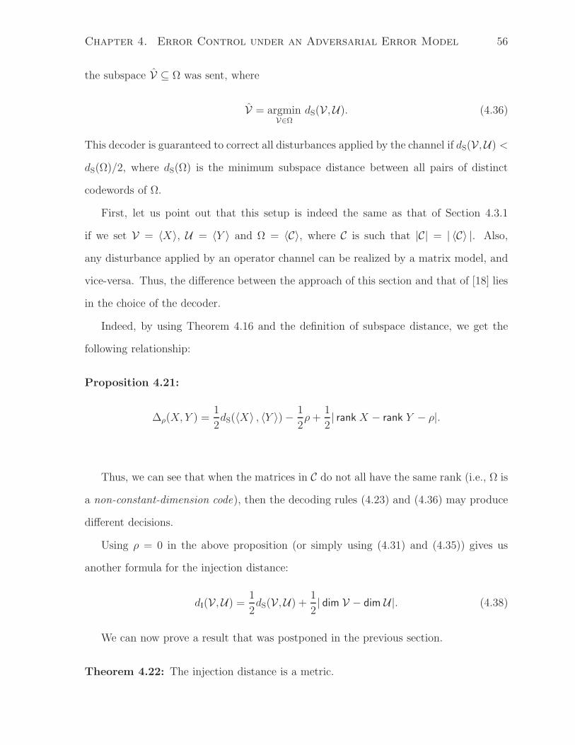
Chapter 4. Error Control under an Adversarial Error Model 56
the subspace V ⊆ Ω was sent, where
V = argminV∈Ω
dS(V,U). (4.36)
This decoder is guaranteed to correct all disturbances applied by the channel if dS(V,U) <
dS(Ω)/2, where dS(Ω) is the minimum subspace distance between all pairs of distinct
codewords of Ω.
First, let us point out that this setup is indeed the same as that of Section 4.3.1
if we set V = 〈X〉, U = 〈Y 〉 and Ω = 〈C〉, where C is such that |C| = | 〈C〉 |. Also,
any disturbance applied by an operator channel can be realized by a matrix model, and
vice-versa. Thus, the difference between the approach of this section and that of [18] lies
in the choice of the decoder.
Indeed, by using Theorem 4.16 and the definition of subspace distance, we get the
following relationship:
Proposition 4.21:
∆ρ(X, Y ) =1
2dS(〈X〉 , 〈Y 〉) − 1
2ρ +
1
2| rank X − rank Y − ρ|.
Thus, we can see that when the matrices in C do not all have the same rank (i.e., Ω is
a non-constant-dimension code), then the decoding rules (4.23) and (4.36) may produce
different decisions.
Using ρ = 0 in the above proposition (or simply using (4.31) and (4.35)) gives us
another formula for the injection distance:
dI(V,U) =1
2dS(V,U) +
1
2| dim V − dim U|. (4.38)
We can now prove a result that was postponed in the previous section.
Theorem 4.22: The injection distance is a metric.

Chapter 4. Error Control under an Adversarial Error Model 57
Proof: Since dS(·, ·) is a metric on P(Fmq ) and | · | is a norm on R, it follows from (4.38)
that dI(·, ·) is also a metric on P(Fmq ).
We now examine in more detail an example situation where the minimum-subspace-
distance decoder and the minimum-discrepancy decoder produce different decisions.
Example 4.4: For simplicity, assume ρ = 0. Consider a subspace code that contains
two codewords V1 = 〈X1〉 and V2 = 〈X2〉 such that γ , dim V2 − dim V1 satisfies d/3 <
γ < d/2, where d , dS(V1,V2).
Suppose the received subspace U = 〈Y 〉 is such that V1 ⊆ U ⊆ V1 + V2 and dim U =
dim V1 +γ = dim V2, as illustrated in Fig. 4.1. Then dS(V1,U) = γ and dS(V2,U) = d−γ,
while Proposition (4.21) gives ∆ρ(X1, Y ) = γ and ∆ρ(X2, Y ) = (d − γ)/2 , ǫ. Since, by
assumption, d − γ > γ and ǫ < γ, it follows that dS(V1,U) < dS(V2,U) but ∆ρ(X1, Y ) >
∆ρ(X2, Y ), i.e., the decoders (4.36) and (4.23) will produce different decisions.
This situation can be intuitively explained as follows. The decoder (4.36) favors the
subspace V1, which is closer in subspace distance to U than V2. However, since V1 is
low-dimensional, U can only be produced from V1 by the insertion of γ dimensions.
The decoder (4.23), on the other hand, favors V2, which, although farther in subspace
distance, can produce U after the replacement of ǫ < γ dimensions. Since one packet
error must occur for each inserted or replaced dimension, we conclude that the decoder
(4.23) finds the solution that minimizes the number of packet errors observed.
Remark: The subspace metric of [18] treats insertions and deletions of dimensions
(called in [18] “errors” and “erasures”, respectively) symmetrically. However, depending
upon the position of the adversary in the network (namely, if there is a source-destination
min-cut between the adversary and the destination) then a single error packet may cause
the replacement of a dimension (i.e., a simultaneous “error” and “erasure” in the termi-
nology of [18]). The injection distance, which is designed to “explain” a received subspace
with as few error-packet injections as possible, properly accounts for this phenomenon,
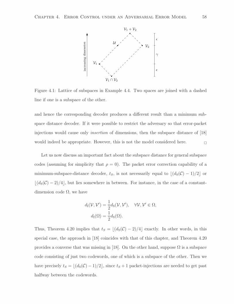
Chapter 4. Error Control under an Adversarial Error Model 58
V2
V1
V1 ∩ V2
V1 + V2
U
ǫ
γ
ǫincre
asi
ng
dim
ensi
on
Figure 4.1: Lattice of subspaces in Example 4.4. Two spaces are joined with a dashed
line if one is a subspace of the other.
and hence the corresponding decoder produces a different result than a minimum sub-
space distance decoder. If it were possible to restrict the adversary so that error-packet
injections would cause only insertion of dimensions, then the subspace distance of [18]
would indeed be appropriate. However, this is not the model considered here.
Let us now discuss an important fact about the subspace distance for general subspace
codes (assuming for simplicity that ρ = 0). The packet error correction capability of a
minimum-subspace-distance decoder, tS, is not necessarily equal to ⌊(dS(C) − 1)/2⌋ or
⌊(dS(C) − 2)/4⌋, but lies somewhere in between. For instance, in the case of a constant-
dimension code Ω, we have
dI(V,V ′) =1
2dS(V,V ′), ∀V,V ′ ∈ Ω,
dI(Ω) =1
2dS(Ω).
Thus, Theorem 4.20 implies that tS = ⌊(dS(C) − 2)/4⌋ exactly. In other words, in this
special case, the approach in [18] coincides with that of this chapter, and Theorem 4.20
provides a converse that was missing in [18]. On the other hand, suppose Ω is a subspace
code consisting of just two codewords, one of which is a subspace of the other. Then we
have precisely tS = ⌊(dS(C)− 1)/2⌋, since tS + 1 packet-injections are needed to get past
halfway between the codewords.

Chapter 4. Error Control under an Adversarial Error Model 59
Since no single quantity is known that perfectly describes the packet error correction
capability of the minimum-subspace-distance decoder (4.36) for general subspace codes,
we cannot provide a definitive comparison between decoders (4.36) and (4.23). However,
we can still compute bounds for codes that fit into Example 4.4.
Example 4.5: Let us continue with Example 4.4. Now, we adjoin another codeword
V3 = 〈X3〉 such that dS(V1,V3) = d and where γ′ , dim V3 − dim V1 satisfies d/3 < γ′ <
d/2. Also we assume that dS(V2,V3) is sufficiently large so as not to interfere with the
problem (e.g., dS(V2,V3) > 3d/2).
Let tS and tM denote the packet error correction capabilities of the decoders (4.36)
and (4.23), respectively. From the argument of Example 4.4, we get tM ≥ maxǫ, ǫ′,
while tS < minǫ, ǫ′, where ǫ′ = (d − γ′)/2. By choosing γ ≈ d/3 and γ′ ≈ d/2, we
get ǫ ≈ d/3 and ǫ′ ≈ d/4. Thus, tM ≥ (4/3)tS, i.e., we obtain a 1/3 increase in error
correction capability by using the decoder (4.23).
4.3.3 Near-Optimality of Liftings of MRD Codes
Unlike the coherent case, where optimal codes can be easily constructed, it seems a hard
combinatorial problem to achieve optimality for noncoherent network coding. So far, no
nontrivial optimal codes are known for either the injection or the subspace metric. Even
in the constant-dimension case, only very simple optimal codes (with very low rate) are
known [52]. Nevertheless, it is a natural question to ask whether MRD codes can be
adapted to noncoherent network coding, and if so, what their relative performance is.
In this subsection, we propose a class of subspace codes that can be easily constructed
from MRD codes and achieve nearly optimal performance.
Lifting Construction
Assume m = n + m′, where m′ ≥ 0. Let I = In×n.

Chapter 4. Error Control under an Adversarial Error Model 60
Definition 4.3: Let the function Π: Fn×m′
q → P(Fn+m′
q ) be given by x 7→ Π(x) =
〈[I x]〉. The subspace Π(x) is called the lifting of the matrix x. Similarly, define the
lifting of the matrix code C ⊆ Fn×m′
q , denoted Π(C), as the subspace code obtained by
lifting each codeword of C.
Definition 4.3 provides an injective mapping between matrix codes and subspace
codes. Note that a subspace code constructed by lifting is always a constant-dimension
code, with codeword dimension n.
The next proposition shows that rank-metric codes are a natural choice of codes in
which to apply the lifting construction.
Proposition 4.23: Let C ⊆ Fn×m′
q and x, x′ ∈ C. Then
dI(Π(x), Π(x′)) = dR(x, x′)
dI(Π(C)) = dR(C).
Proof: We have
dI(Π(x), Π(x′)) = dim(Π(x) + Π(x′)) − mindim Π(x), dim Π(x′)
= rank
I x
I x′
− n
= rank
I x
0 x′ − x
− n
= rank(x′ − x).
The second statement is immediate.
Proposition 4.23 shows that a subspace code constructed by lifting inherits the dis-
tance properties of its underlying rank-metric code. It follows that a subspace code

Chapter 4. Error Control under an Adversarial Error Model 61
Ω ⊆ Pn(Fn+m′
q ) with constant dimension n, minimum injection distance d and cardinal-
ity
|Ω| = qmaxn,m′(minn,m′−d+1) (4.39)
can be constructed as the lifting Ω = Π(C) of an MRD code C ∈ Fn×m′
q with minimum
rank distance d.
In this context, it is worth mentioning that the Reed-Solomon-like constant-dimension
codes proposed in [18] correspond exactly to the lifting of Gabidulin codes.
Performance
We now investigate whether such liftings of MRD codes are really “good” in terms of the
injection metric. We start with some results on the size of optimal subspace codes.
Let Aq(m, d, n) denote the size of a largest subspace code in Pmaxn (Fm
q ) with minimum
injection distance d. Similarly, let Bq(m, d, n) denote the size of a largest constant-
dimension code in Pn(Fmq ) with minimum injection distance d.
It is shown in [53] that, for 1 ≤ d ≤ n,
Bq(m, d, n) ≤[
mn−d+1
]
[n
n−d+1
] .
It follows from (2.12) that, for 1 ≤ d ≤ n,
Bq(m, d, n) ≤ 4q(m−n)(n−d+1).
Note that Bq(m, d, n) = 1 for d > n.
A very simple bound on Aq(m, d, n) can be obtained by noticing that Pmaxn (Fm
q ) =
Pn(Fmq ) ∪ Pmax
n−1(Fmq ). Thus,
Aq(m, d, n) ≤ Bq(m, d, n) + Aq(m, d, n − 1).

Chapter 4. Error Control under an Adversarial Error Model 62
Iterating the bound, and using the fact that Bq(m, d, k) is nondecreasing for 0 ≤ k ≤ m/2,
we have, for n ≤ m/2,
Aq(m, d, n) ≤ Bq(m, d, n) + Bq(m, d, n − 1) + · · ·+ Bq(m, d, 0)
≤ Bq(m, d, n) + nBq(m, d, n − 1)
≤ 4q(m−n)(n−d+1) + 4nq(m−n+1)(n−d). (4.43)
For a subspace code Ω ⊆ Pmaxn (Fm
q ) with dI(Ω) = d, let
α(Ω) ,logq Aq(m, d, n) − logq |Ω|
logq Aq(m, d, n)
denote the rate loss incurred when using Ω rather than an optimal subspace code.
The following theorem shows that liftings of MRD codes are asymptotically optimal
for large packet sizes.
Theorem 4.24: Let Ω ⊆ Pmaxn (Fm
q ) be the lifting of an MRD code with m ≥ 2n and
dI(Ω) = d. Then
α(Ω) ≤ 1
(m − n)(n − d + 1)
(2
log2 q+
n
qm−2n+d ln q
)
≤ 4
P+
1
2P/2 ln 2
where P = m log2 q is the packet size in bits.

Chapter 4. Error Control under an Adversarial Error Model 63
Proof: We have
α(Ω) ≤ logq Aq(m, d, n) − logq |Ω|logq |Ω|
=1
logq |Ω|logq
(Aq(m, d, n)
|Ω|
)
≤ 1
logq |Ω|logq
(4q(m−n)(n−d+1) + 4nq(m−n+1)(n−d)
|Ω|
)
(4.46)
=1
(m − n)(n − d + 1)
(
logq 4 + logq
(
1 +nq(m−n+1)(n−d)
q(m−n)(n−d+1)
))
(4.47)
=1
(m − n)(n − d + 1)
(logq 4 + logq
(1 + nq2n−m−d
))
≤ 1
(m − n)(n − d + 1)
(
logq 4 +nq2n−m−d
ln q
)
(4.48)
≤ 1
(m − n)(n − d + 1)
(2
log2 q+
n
qm−2n+d ln q
)
(4.49)
where (4.46) follows from (4.39), (4.47) follows from (4.43), and (4.48) follows from the
fact that ln(1 + x) ≤ x. Let fn(d) denote the RHS of (4.48). Since fn(d) is a convex
function of d for 1 ≤ d ≤ n, it is maximized at one of the boundaries, i.e., either fn(1)
or fn(n). Let L = max1≤n≤m/2 fn(1) and U = max1≤n≤m/2 fn(n) . We now show that
U ≥ L.
Clearly, since fn(n) is an increasing function of n, it is maximized at n = m/2. We
have
U = fm/2(m/2) =1
m/2
(2
log2 q+
m/2
qm/2 ln q
)
=4
P+
1
2P/2 ln q
Since m = 2, 3 forces L = f1(1) = U , it suffices to assume m ≥ 4. A simple evaluation

Chapter 4. Error Control under an Adversarial Error Model 64
shows that L = maxf1(1), f2(1) < U for m = 4, so we assume that m ≥ 5. We have
fn(1) =2
(m − n)n log2 q+
1
(m − n)qm−2n+1 ln q
≤ 2
(m − n)n log2 q+
1
(m/2)q ln q
≤ 2
(m − 1) log2 q+
1
(m/2)q ln q
=2m
(m − 1)P+
2
Pq ln 2
≤ 1
P
(2m
(m − 1)+
1
ln 2
)
≤ 4
Pfor m ≥ 5.
Thus, L ≤ U for all m. It follows that
α(Ω) ≤ U ≤ 4
P+
1
2P/2 ln 2.
Theorem 4.24 shows that, for all practical purposes, liftings of MRD codes are es-
sentially optimal. Indeed, for packet sizes of more than 400 bits, the rate loss is smaller
than 1%.
4.4 Equivalence of Coherent and Noncoherent De-
coding Problems
We have seen in Section 4.2.1 that, for coherent network coding, the minimum-discrepancy
decoding problem is given by
Xcoh = argminX∈C
rank(Ycoh − AcohX) (4.52)
where C ⊆ Fn×mq is the code, Acoh ∈ FN×n
q is the (known) transfer matrix, and Ycoh ∈
FN×mq is the received matrix.
For noncoherent network coding, the minimum-discrepancy decoding problem has, in
general, quite a different nature. However, consider the case of a lifted code. Specifically,
let C ⊆ Fn×mq be a rank-metric code, and suppose that each transmitted matrix X has the
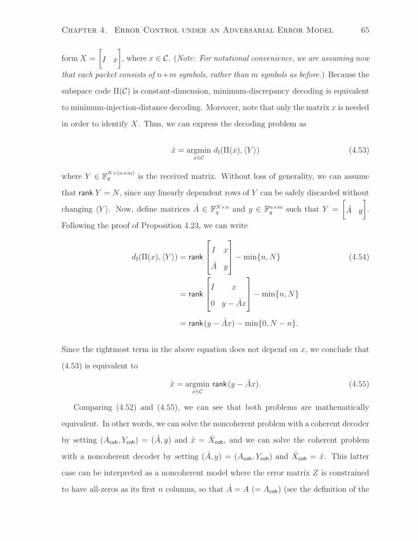
Chapter 4. Error Control under an Adversarial Error Model 65
form X =
[
I x
]
, where x ∈ C. (Note: For notational convenience, we are assuming now
that each packet consists of n+m symbols, rather than m symbols as before.) Because the
subspace code Π(C) is constant-dimension, minimum-discrepancy decoding is equivalent
to minimum-injection-distance decoding. Moreover, note that only the matrix x is needed
in order to identify X. Thus, we can express the decoding problem as
x = argminx∈C
dI(Π(x), 〈Y 〉) (4.53)
where Y ∈ FN×(n+m)q is the received matrix. Without loss of generality, we can assume
that rank Y = N , since any linearly dependent rows of Y can be safely discarded without
changing 〈Y 〉. Now, define matrices A ∈ FN×nq and y ∈ Fn×m
q such that Y =
[
A y
]
.
Following the proof of Proposition 4.23, we can write
dI(Π(x), 〈Y 〉) = rank
I x
A y
− minn, N (4.54)
= rank
I x
0 y − Ax
− minn, N
= rank(y − Ax) − min0, N − n.
Since the rightmost term in the above equation does not depend on x, we conclude that
(4.53) is equivalent to
x = argminx∈C
rank(y − Ax). (4.55)
Comparing (4.52) and (4.55), we can see that both problems are mathematically
equivalent. In other words, we can solve the noncoherent problem with a coherent decoder
by setting (Acoh, Ycoh) = (A, y) and x = Xcoh, and we can solve the coherent problem
with a noncoherent decoder by setting (A, y) = (Acoh, Ycoh) and Xcoh = x. This latter
case can be interpreted as a noncoherent model where the error matrix Z is constrained
to have all-zeros as its first n columns, so that A = A (= Acoh) (see the definition of the

Chapter 4. Error Control under an Adversarial Error Model 66
LNCC). With this understanding, we will from now on consider only the noncoherent
decoding problem.
In the next chapter, we will look for computationally efficient approaches to solving
(4.55).

Chapter 5
Generalized Decoding of
Rank-Metric Codes
The objective of this chapter is to develop an approach to solving (4.55) that can exploit
the structure of rank-metric codes.
It is important to note that a different algorithm for solving (4.55) has been previously
proposed in [18] for the case where the rank-metric code is a Gabidulin code. This
algorithm is based on Sudan-style list decoding methods and can be performed in O(n3m)
operations in Fq. On one hand, the literature on rank-metric codes suggests that faster
decoding algorithms should be possible; on the other hand, it is not obvious how to
reconcile the theory of rank-metric codes and our decoding problem (4.55). Thus, the
goal of this chapter is to propose a rank-metric approach to solving (4.55). As we will
see in Chapter 6, this approach indeed allows much faster decoding algorithms, with
complexity O(d2nm + n2m).
In Section 5.1, we propose a generalized rank-metric decoding problem that captures
both (4.55) and the conventional rank-metric decoding problem (2.22). In Section 5.2 we
propose a coding-theoretic perspective on this problem. We show that the generalized
problem differs from the conventional problem by the fact that partial information is
67

Chapter 5. Generalized Decoding of Rank-Metric Codes 68
available about the error word. This partial information may be in the form of erasures
(knowledge of an error location but not its value) and deviations (knowledge of an error
value but not its location). As we show in Section 5.3, taking erasures and deviations
into account (when they occur) is strictly necessary for appropriately solving (4.55).
5.1 Problem Formulation
5.1.1 Motivation
The problem we are interested in solving, (4.55), looks quite similar to a conventional
rank-metric decoder problem. Indeed, (2.22) is the special case of (4.55) where A is an
identity matrix. Since both problems are similar, and efficient techniques already exist
for solving (2.22), one might wonder if (4.55) can be solved by the same techniques for
(2.22). The goal of this section is to reformulate (4.55) in order to make this possible.
A naive approach would be to consider the auxiliary code CA = Ax, x ∈ C. Then,
(4.55) can be reexpressed as the conventional rank-metric decoding problem
x′ = minx′∈C
A
rank(y − x′) (5.1)
where any x ∈ x | Ax = x′ is a solution to (4.55).
Although conceptually simple, this approach can only be computationally efficient if
an efficient decoder for CA (for every admissible A) is readily available at the decoder.
This requirement is likely to render the approach infeasible to implement in practice.
This is especially true for noncoherent network coding, since the matrix A—which could
be any—is only known at the time of decoding.
For this reason, we seek to reformulate the decoding problem in such a way that
the structure of the code C can be exploited. Roughly speaking, we should attempt to
manipulate y rather than x in the expression for (4.55).
Let us first consider a special case. Suppose N = n and A is invertible. Then we can

Chapter 5. Generalized Decoding of Rank-Metric Codes 69
write
rank(y − Ax) = rank A−1(y − Ax) = rank(r − x)
where r = A−1y. In this case, (4.55) becomes precisely a conventional decoding problem
for the rank-metric code C, with received word r ∈ Fn×mq .
In general, however, the matrix A may not be invertible. The next subsection presents
our approach to this general case.
5.1.2 The Reduction Transformation
Let µ = n − rank A and let δ = rank Y − rank A. Recall that Y =
[
A y
]
is assumed to
be a matrix with full row rank. It follows that µ and δ = N − rank A give the row- and
column-rank deficiencies of A. The essence of our approach lies in converting Y (through
row operations) into a form that resembles X =
[
I x
]
; for instance, into Y = [I r] as
in the special case above. Then we can hope to (partially) cancel out the left portion of
Y when computing (4.54).
Before proceeding, let us define a convenient notation. Let dflip : Fn×µq → Fµ×n
q be
given by (dflip(L))i,j = Lµ−j+1,n−i+1. That is, dflip(·) flips a matrix along its main diago-
nal, by exchanging its bottom-right and top-left corners (analogously to the transpose).
Let us now describe the steps of our proposed transformation.
Step 1: Convert Y to reduced row echelon form
Let RRE (Y ) denote the reduced row echelon form of Y . For i = 1, . . . , N , let pi be
the column position of the leading entry of row i in RRE (Y ). Let U c = p1, . . . , pn−µ
and U = 1, . . . , n \ U c. Note that |U| = µ.
Step 2: Insert µ all-zero rows
Let p0 = 0. Let Y be a matrix constructed by inserting all-zero rows in certain
positions of RRE (Y ). Namely, for i = 1, . . . , n − µ, insert pi − pi−1 − 1 all-zero rows
just before the ith row, and insert further n− pn−µ all-zero rows just after the (n− µ)th

Chapter 5. Generalized Decoding of Rank-Metric Codes 70
row. The resulting matrix Y will have all-zero rows precisely in the positions indexed by
U , and the columns indexed by U c will coincide with those of an identity matrix. More
precisely, Y will be an (n + δ) × (n + m) matrix of the form
Y =
J r
0 V
where J ∈ Fn×nq , r ∈ Fn×m
q and V ∈ Fδ×mq satisfy
ITU
[
J r
]
= 0 (5.4)
JIUc = IUc (5.5)
RRE(V ) = V (5.6)
rank V = δ. (5.7)
Step 3: Extract matrices r, L, V
Note that JIUc = IUc implies (J − I)IUc = 0. This means that the columns of J − I
indexed by U c are all-zero (or, equivalently, only the columns indexed by U are nonzero).
Thus, we can write J − I = LITU , for some L ∈ Fn×µ
q . Note that, by construction, L is
such that dflip(−L) is in RRE form. Finally, we can express Y as
Y =
I + LITU r
0 V
. (5.8)
Note that Y has the same row space as Y .
The tuple (r, L, V ) ∈ Fn×mq × Fn×µ
q × Fδ×mq obtained by the above procedure is called
a reduction of the matrix Y . Since we are really only interested in the row space of Y ,
we may also call (r, L, V ) a reduction of the subspace 〈Y 〉.
Remark: The set U is not included in the definition of reduction since it can be easily
obtained from L: each element of U corresponds to the row position of the last nonzero
entry of a column of L. (This holds because dflip(−L) is in RRE form.) Thus, every

Chapter 5. Generalized Decoding of Rank-Metric Codes 71
subspace is mapped to a unique reduction and every reduction uniquely identifies a
subspace.
Example 5.1: Let q = 7, n = m = 5 and suppose
Y =
[
A y
]
=
3 0 4 5 4 4 6 2 3 5
1 5 5 3 5 4 0 1 2 6
4 3 1 6 1 0 4 3 1 0
5 6 5 5 1 4 2 1 3 1
6 2 2 4 4 6 6 0 1 2
. (5.9)
Note that rank Y = N = 5, while rank A = 4, i.e., µ = δ = 1. We first convert Y to RRE
form to obtain
RRE (Y ) =
1 0 6 0 0 0 4 2 3 1
0 1 4 0 0 0 4 6 2 5
0 0 0 1 0 0 1 4 2 3
0 0 0 0 1 0 5 2 6 5
0 0 0 0 0 1 1 6 4 4
.
Note that U = 3. After inserting µ = 1 all-zero row in the appropriate place, we obtain
Y =
1 0 6 0 0 0 4 2 3 1
0 1 4 0 0 0 4 6 2 5
0 0 0 0 0 0 0 0 0 0
0 0 0 1 0 0 1 4 2 3
0 0 0 0 1 0 5 2 6 5
0 0 0 0 0 1 1 6 4 4
.

Chapter 5. Generalized Decoding of Rank-Metric Codes 72
We can now extract matrices (recall that −1 = 6 in F7)
L =
6
4
6
0
0
r =
0 4 2 3 1
0 4 6 2 5
0 0 0 0 0
0 1 4 2 3
0 5 2 6 5
V =
[
1 1 6 4 4
]
such that (5.8) is satisfied. Thus, (r, L, V ) is a reduction of Y .
It is worth mentioning that if Π(x) is the lifting of x, then (x, [ ], [ ]) is the reduction
of Π(x). That is, reduction can be interpreted as the inverse of lifting.
We can now prove the main result of this section.
Theorem 5.1: Let (r, L, V ) ∈ Fn×mq × Fn×µ
q × Fδ×mq be a reduction of Y . Then
dI(Π(x), 〈Y 〉) = rank
r − x L
V 0
− minµ, δ.
Proof: Let U be a set consistent with the reduction transformation, and let J = I+LITU .
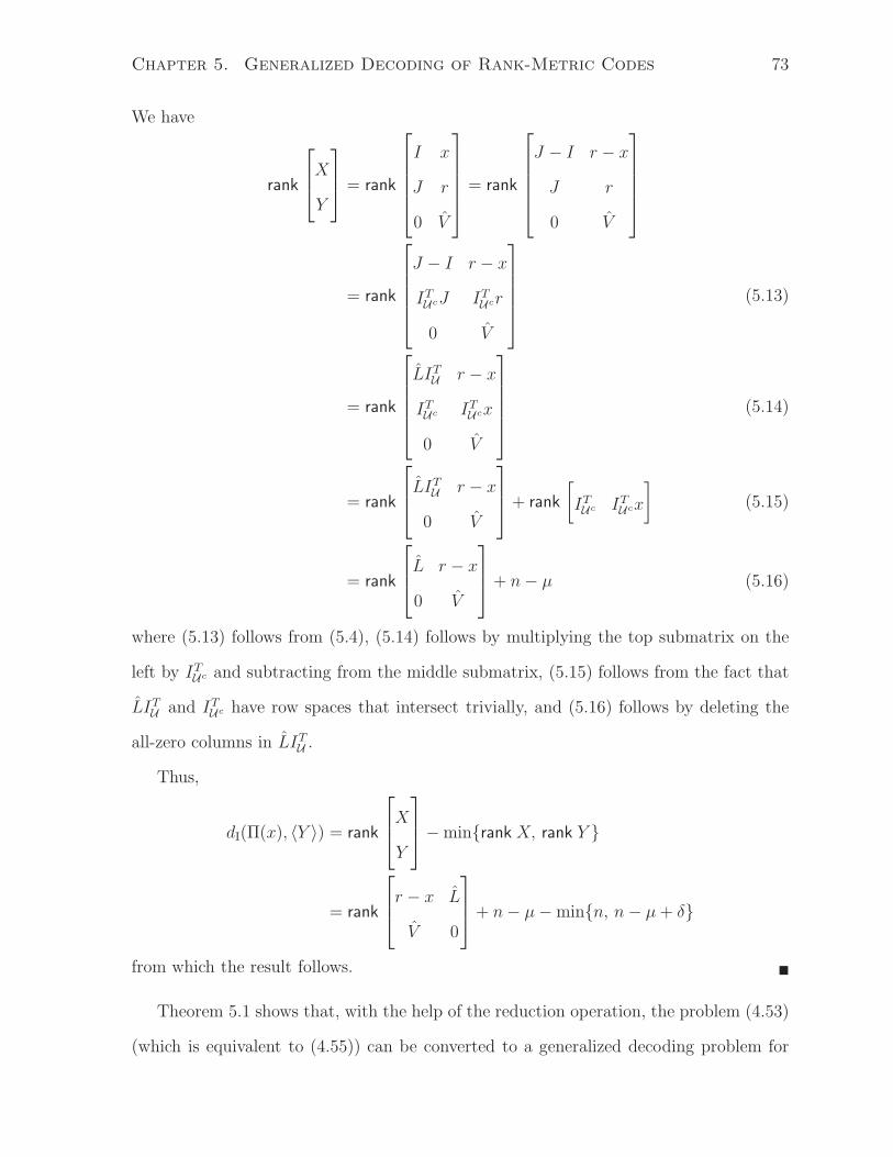
Chapter 5. Generalized Decoding of Rank-Metric Codes 73
We have
rank
X
Y
= rank
I x
J r
0 V
= rank
J − I r − x
J r
0 V
= rank
J − I r − x
ITUcJ IT
Ucr
0 V
(5.13)
= rank
LITU r − x
ITUc IT
Ucx
0 V
(5.14)
= rank
LITU r − x
0 V
+ rank
[
ITUc IT
Ucx
]
(5.15)
= rank
L r − x
0 V
+ n − µ (5.16)
where (5.13) follows from (5.4), (5.14) follows by multiplying the top submatrix on the
left by ITUc and subtracting from the middle submatrix, (5.15) follows from the fact that
LITU and IT
Uc have row spaces that intersect trivially, and (5.16) follows by deleting the
all-zero columns in LITU .
Thus,
dI(Π(x), 〈Y 〉) = rank
X
Y
− minrank X, rank Y
= rank
r − x L
V 0
+ n − µ − minn, n − µ + δ
from which the result follows.
Theorem 5.1 shows that, with the help of the reduction operation, the problem (4.53)
(which is equivalent to (4.55)) can be converted to a generalized decoding problem for

Chapter 5. Generalized Decoding of Rank-Metric Codes 74
the rank-metric code C. Notably, the structure of the code is preserved in this new
formulation. The problem is summarized below.
Generalized Rank-Metric Decoding: Let C ⊆ Fn×mq be a rank-metric code. Given a
tuple (r, L, V ) ∈ Fn×mq × Fn×µ
q × Fδ×mq with rank L = µ and rank V = δ, compute
x = argminx∈C
rank
r − x L
V 0
. (5.17)
Note that, when µ = δ = 0, we recover precisely the conventional rank-metric decod-
ing problem (2.22).
5.2 A Coding Theory Perspective
In this section, we develop a perspective on the generalized rank-metric decoding problem
that proves useful to the understanding of the correction capability of rank-metric codes,
as well as to the formulation of an efficient decoding algorithm.
5.2.1 Error Locations and Error Values
Let C ∈ Fn×mq be a rank-metric code. For a transmitted codeword x and a received word
r, define e , r − x as the error word.
Note that if an error word e has rank τ , then we can write e = LV for some full-rank
matrices L ∈ Fn×τq and V ∈ Fτ×m
q , as in (2.1). Let L1, . . . , Lτ ∈ Fnq denote the columns of
L and let V1, . . . , Vτ ∈ F1×mq denote the rows of V . Then we can expand e as a summation
of outer products
e = LV =
τ∑
j=1
LjVj. (5.18)
We will now borrow some terminology from classical coding theory. Recall that an

Chapter 5. Generalized Decoding of Rank-Metric Codes 75
error vector e ∈ Fnq of Hamming weight τ can be expanded uniquely as a sum of products
e =
τ∑
j=1
Iijej
where 1 ≤ i1 < · · · < iτ ≤ n and e1, . . . , eτ ∈ Fq. The index ij (or the unit vector Iij )
specifies the location of the jth error, while ej specifies the value of the jth error.
Analogously, in the sum-of-outer-products expansion (5.18) we will refer to L1, . . . , Lτ
as the error locations and to V1, . . . , Vτ as the error values. The location Lj (a column
vector) indicates that, for i = 1, . . . , n, the jth error value Vj (a row vector) occurred in
row i multiplied by the coefficient Lij . Of course, Lij = 0 means that the jth error value
is not present in row i.
Note that, in contrast to the classical case, the distinction between error locations
and error values in the rank metric is merely a convention. If we prefer to think of
errors as occurring on columns rather than rows, then the roles of Lj and Vj would be
interchanged. The same observation will also apply to any concept derived from the
interpretation of these quantities as error locations and error values.
It is important to mention that, in contrast with classical coding theory, the expansion
(5.18) is not unique, since
e = LV = LT−1TV
for any nonsingular T ∈ Fτ×τq . Thus, strictly speaking, L1, . . . , Lτ and V1, . . . , Vτ are just
one possible set of error locations/values describing the error word e.
5.2.2 Erasures and Deviations
We now reformulate the generalized rank-metric decoding problem in a way that facili-
tates its understanding and solution.
First, observe that the problem (5.17) is equivalent to the problem of finding an error
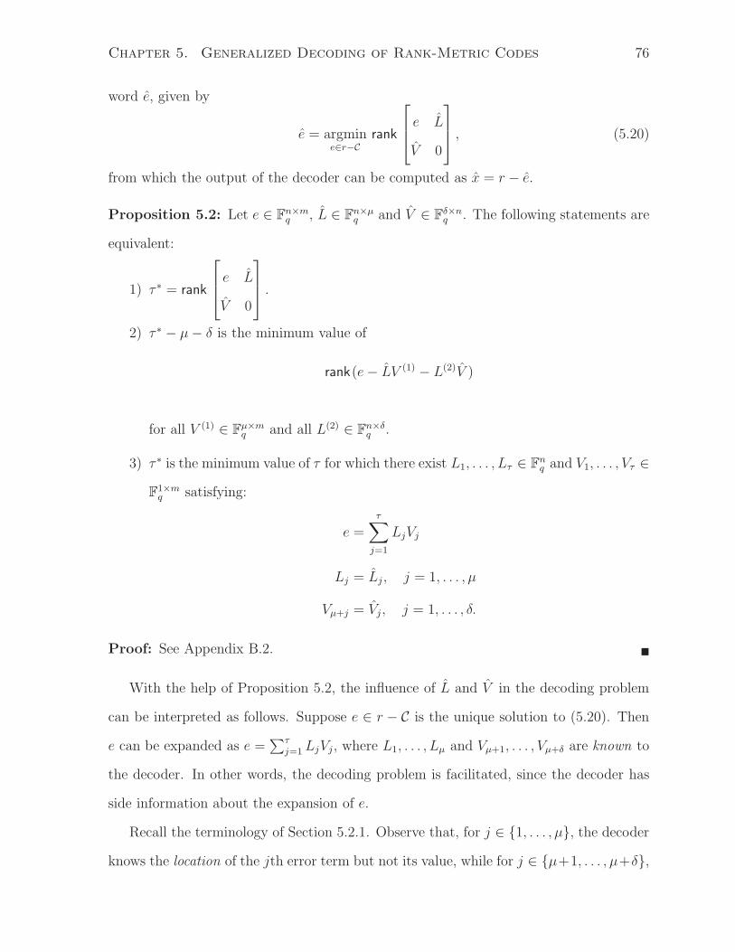
Chapter 5. Generalized Decoding of Rank-Metric Codes 76
word e, given by
e = argmine∈r−C
rank
e L
V 0
, (5.20)
from which the output of the decoder can be computed as x = r − e.
Proposition 5.2: Let e ∈ Fn×mq , L ∈ Fn×µ
q and V ∈ Fδ×nq . The following statements are
equivalent:
1) τ ∗ = rank
e L
V 0
.
2) τ ∗ − µ − δ is the minimum value of
rank(e − LV (1) − L(2)V )
for all V (1) ∈ Fµ×mq and all L(2) ∈ Fn×δ
q .
3) τ ∗ is the minimum value of τ for which there exist L1, . . . , Lτ ∈ Fnq and V1, . . . , Vτ ∈
F1×mq satisfying:
e =τ∑
j=1
LjVj
Lj = Lj , j = 1, . . . , µ
Vµ+j = Vj, j = 1, . . . , δ.
Proof: See Appendix B.2.
With the help of Proposition 5.2, the influence of L and V in the decoding problem
can be interpreted as follows. Suppose e ∈ r − C is the unique solution to (5.20). Then
e can be expanded as e =∑τ
j=1 LjVj, where L1, . . . , Lµ and Vµ+1, . . . , Vµ+δ are known to
the decoder. In other words, the decoding problem is facilitated, since the decoder has
side information about the expansion of e.
Recall the terminology of Section 5.2.1. Observe that, for j ∈ 1, . . . , µ, the decoder
knows the location of the jth error term but not its value, while for j ∈ µ+1, . . . , µ+δ,
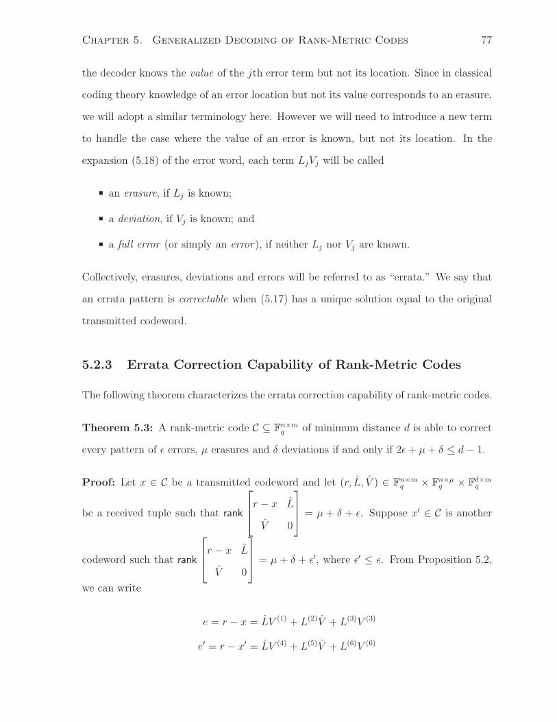
Chapter 5. Generalized Decoding of Rank-Metric Codes 77
the decoder knows the value of the jth error term but not its location. Since in classical
coding theory knowledge of an error location but not its value corresponds to an erasure,
we will adopt a similar terminology here. However we will need to introduce a new term
to handle the case where the value of an error is known, but not its location. In the
expansion (5.18) of the error word, each term LjVj will be called
an erasure, if Lj is known;
a deviation, if Vj is known; and
a full error (or simply an error), if neither Lj nor Vj are known.
Collectively, erasures, deviations and errors will be referred to as “errata.” We say that
an errata pattern is correctable when (5.17) has a unique solution equal to the original
transmitted codeword.
5.2.3 Errata Correction Capability of Rank-Metric Codes
The following theorem characterizes the errata correction capability of rank-metric codes.
Theorem 5.3: A rank-metric code C ⊆ Fn×mq of minimum distance d is able to correct
every pattern of ǫ errors, µ erasures and δ deviations if and only if 2ǫ + µ + δ ≤ d − 1.
Proof: Let x ∈ C be a transmitted codeword and let (r, L, V ) ∈ Fn×mq × Fn×µ
q × Fδ×mq
be a received tuple such that rank
r − x L
V 0
= µ + δ + ǫ. Suppose x′ ∈ C is another
codeword such that rank
r − x L
V 0
= µ + δ + ǫ′, where ǫ′ ≤ ǫ. From Proposition 5.2,
we can write
e = r − x = LV (1) + L(2)V + L(3)V (3)
e′ = r − x′ = LV (4) + L(5)V + L(6)V (6)

Chapter 5. Generalized Decoding of Rank-Metric Codes 78
for some V (1), L(2), . . . , V (6) with appropriate dimensions such that rank L(3)V (3) = ǫ and
rank L(6)V (6) = ǫ′.
Thus,
e − e′ = L(V (1) − V (4)) + (L(2) − L(5))V + L(3)V (3) + L(6)V (6)
and
rank(x′ − x) = rank(e − e′) ≤ µ + δ + ǫ + ǫ′ ≤ d − 1
contradicting the minimum distance of the code.
Conversely, let x, x′ ∈ C be two codewords such that rank(x′ − x) = d. For all µ, δ
and ǫ such that µ + δ + 2ǫ ≥ d, we can write
x′ − x = L(1)V (1) + L(2)V (2) + L(3)V (3) + L(4)V (4)
where the four terms above have inner dimensions equal to µ, δ, ǫ and ǫ′ = d−µ− δ− ǫ,
respectively. Let
e = L(1)V (1) + L(2)V (2) + L(3)V (3)
e′ = −L(4)V (4)
and observe that x′−x = e−e′. Let r = x+e = x′+e′, L = L(1) and V = V (2). Suppose
that x is transmitted and the tuple (r, L, V ) is received. Then
rank
r − x L
V 0
= rank
e L
V 0
= µ + δ + ǫ
rank
r − x′ L
V 0
= rank
e′ L
V 0
= µ + δ + ǫ′.
Since ǫ′ = d−µ− δ − ǫ ≤ ǫ, it follows that x cannot be the unique solution to (5.17) and
therefore the errata pattern cannot be corrected.

Chapter 5. Generalized Decoding of Rank-Metric Codes 79
Theorem 5.3 shows that, similarly to erasures in the Hamming metric, erasures and
deviations cost half of an error in the rank metric.
Theorem 5.3 also shows that taking into account information about erasures and
deviations (when they occur) can strictly increase the error correction capability of a
rank-metric code. Indeed, suppose that an error word of rank t = µ + δ + ǫ is applied
to a codeword, where µ, δ and ǫ are the number of erasures, deviations and full errors,
respectively, in the errata pattern. It follows that a conventional rank decoder (which
ignores the information about erasures and deviations) can only guarantee successful
decoding if 2t ≤ d− 1, where d is the minimum rank distance of the code. On the other
hand, a generalized rank decoder requires only 2ǫ + µ + δ ≤ d− 1, or 2t ≤ d− 1 + µ + δ,
in order to guarantee successful decoding. In this case, the error correction capability is
increased by (µ+δ)/2 if a generalized rank decoder is used instead of a conventional one.
5.2.4 Comparison with Previous Work
We conclude this chapter by comparing our generalized rank-metric decoding problem
with other decoding problems previously proposed for rank-metric codes.
There has been a significant amount of research on the problem of correcting rank
errors in the presence of “row and column erasures” [54–58], where a row erasure means
that all entries of that row are replaced by an erasure symbol, and similarly for a column
erasure. The decoding problem in this setting is naturally defined as finding a codeword
such that, when the erased entries in the received word are replaced by those of the
codeword, the difference between this new matrix and the codeword has the smallest
possible rank. We now show that this problem is a special case of (5.17).
First, we force the received word r to be in Fn×mq by replacing each erasure symbol
with an arbitrary symbol in Fq, say 0. Suppose that the rows i1, . . . , iµ and the columns
k1, . . . , kδ have been erased. Let L ∈ Fn×µq be given by Lij ,j = 1 and Li,j = 0, ∀i 6= ij ,
for j = 1, . . . , µ and let V ∈ Fδ×mq be given by Vj,kj
= 1 and Vj,k = 0, ∀k 6= kj, for

Chapter 5. Generalized Decoding of Rank-Metric Codes 80
j = 1, . . . , δ. Since
r − x L
V 0
=
r L
V 0
−
x 0
0 0
(5.25)
it is easy to see that we can perform column operations on (5.25) to replace the erased
rows of r with the same entries as x, and similarly we can perform row operations on (5.25)
to replace the erased columns of r with the same entries as x. The decoding problem
(5.17) is unchanged by these operations and reduces exactly to the decoding problem
with “row and column erasures” described in the previous paragraph. An example is
given below.
Example 5.2: Let n = m = 3. Suppose the third row and the second column have been
erased in the received word. Then
r =
r11 0 r13
r21 0 r23
0 0 0
, L =
0
0
1
, V =
[
0 1 0
]
.
Since
r11 0 r13 0
r21 0 r23 0
0 0 0 1
0 1 0 0
and
r11 x12 r13 0
r21 x22 r23 0
x31 x32 x33 1
0 1 0 0

Chapter 5. Generalized Decoding of Rank-Metric Codes 81
are row equivalent, we obtain that
rank
r − x L
V 0
= rank
r11 − x11 0 r13 − x13 0
r21 − x21 0 r23 − x23 0
0 0 0 1
0 1 0 0
= 2 + rank
r11 − x11 0 r13 − x13
r21 − x21 0 r23 − x23
0 0 0
which is essentially the same objective function as in the decoding problem with “row
and column erasures” described above.
While row/column erasures are a special case of erasures/deviations, it also true
that the latter can always be transformed into the former. This can be accomplished by
multiplying all rank-metric codewords to the left and to the right by nonsingular matrices
in such a way that the corresponding Lj and Vj become unit vectors. The drawback of
this approach, as pointed out in Section 5.1.1, is that the structure of the code is changed
at each decoding instance, which may increase complexity and/or raise implementation
issues. Thus, it is probably more advantageous in practice to fix the structure of the
code and construct a decoder that can handle the generalized notions of erasures and
deviations. This is the approach that is taken in Chapter 6.
5.3 Relationship with the Linear Network Coding
Channel
In this section, we relate the concepts of erasures, deviations and full errors to the model
of Section 4.3. More precisely, we determine all possible values for µ, δ and ǫ under that
model.

Chapter 5. Generalized Decoding of Rank-Metric Codes 82
Recall once again that we are assuming that packets consist of n + m symbols. Let
H = 1, . . . , n denote the column positions of the first n entries of a packet (which we
interpret as the packet header). Let YH denote the sub-matrix of Y consisting of the
columns indexed by H. In addition, note that, from the definition of full errors together
with (5.16), we have
ǫ , rank
r − x L
V 0
− µ − δ = rank
X
Y
− n − δ.
Definition 5.1: Let A ∈ FN×nq and X ∈ F
n×(n+m)q be such that XH = I. A tuple (µ, δ, ǫ)
is admissible for (A, X, t) if there exists an output of the LNCC that induces precisely
µ erasures, δ deviations and ǫ full errors; in other words, there exist matrices D ∈ FN×tq
and Z ∈ Ft×(n+m)q such that Y = AX + DZ satisfies
rank YH = n − µ (5.29)
rank Y = n − µ + δ (5.30)
rank
X
Y
= n + δ + ǫ. (5.31)
When A and X are fixed, we may simply say that (µ, δ, ǫ) is admissible for t.
Theorem 5.4: For any A ∈ FN×nq and X ∈ F
n×(n+m)q such that XH = I, a tuple (µ, δ, ǫ)
is admissible for t if and only if
maxρ − t, n − N, 0 ≤ µ ≤ ρ + t
0 ≤ δ ≤ mint, t − ρ + µ, N − n + µ
0 ≤ ǫ ≤ t − maxµ − ρ, δ
where ρ = n − rank A.
Proof: See Appendix B.2.
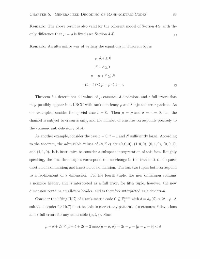
Chapter 5. Generalized Decoding of Rank-Metric Codes 83
Remark: The above result is also valid for the coherent model of Section 4.2, with the
only difference that µ = ρ is fixed (see Section 4.4).
Remark: An alternative way of writing the equations in Theorem 5.4 is
µ, δ, ǫ ≥ 0
δ + ǫ ≤ t
n − µ + δ ≤ N
−(t − δ) ≤ µ − ρ ≤ t − ǫ.
Theorem 5.4 determines all values of µ erasures, δ deviations and ǫ full errors that
may possibly appear in a LNCC with rank deficiency ρ and t injected error packets. As
one example, consider the special case t = 0. Then µ = ρ and δ = ǫ = 0, i.e., the
channel is subject to erasures only, and the number of erasures corresponds precisely to
the column-rank deficiency of A.
As another example, consider the case ρ = 0, t = 1 and N sufficiently large. According
to the theorem, the admissible values of (µ, δ, ǫ) are (0, 0, 0), (1, 0, 0), (0, 1, 0), (0, 0, 1),
and (1, 1, 0). It is instructive to consider a subspace interpretation of this fact. Roughly
speaking, the first three tuples correspond to: no change in the transmitted subspace;
deletion of a dimension; and insertion of a dimension. The last two tuples both correspond
to a replacement of a dimension. For the fourth tuple, the new dimension contains
a nonzero header, and is interpreted as a full error; for fifth tuple, however, the new
dimension contains an all-zero header, and is therefore interpreted as a deviation.
Consider the lifting Π(C) of a rank-metric code C ⊆ Fn×mq with d = dR(C) > 2t+ρ. A
suitable decoder for Π(C) must be able to correct any patterns of µ erasures, δ deviations
and ǫ full errors for any admissible (µ, δ, ǫ). Since
µ + δ + 2ǫ ≤ µ + δ + 2t − 2 maxµ − ρ, δ = 2t + ρ − |µ − ρ − δ| < d

Chapter 5. Generalized Decoding of Rank-Metric Codes 84
it follows that a generalized rank-metric decoder is a suitable decoder for Π(C).
We conclude this chapter by presenting an example that illustrates all the ideas
discussed.
Example 5.3: Let q = 7, let n = m = 5, and let C ⊆ Fn×mq be a rank-metric code with
dR(C) = 5. Consider an LNCC with ρ = 0 and t = 2. Since 2t+ ρ = 4 < dR(C), we know
that the lifting Π(C) is able to guarantee reliable communication.
Suppose that X =
[
I x
]
is transmitted through the LNCC, where
x =
6 3 2 1 6
2 5 0 4 6
5 2 5 0 4
3 5 2 5 0
1 3 5 2 5
is a codeword of C. Let the channel parameters be
A =
3 0 4 5 4
1 5 0 3 5
4 3 6 6 1
5 6 6 5 1
6 2 5 4 4
D =
0 4
2 5
5 2
1 0
3 5
and
Z =
0 0 6 0 0 0 1 2 3 4
0 0 0 0 0 6 2 4 4 0
.
Then the channel output Y = AX + DZ is given precisely by (5.9). The reduction
(r, L, V ) of this matrix was computed in Example 5.1. It follows that there are µ = 1
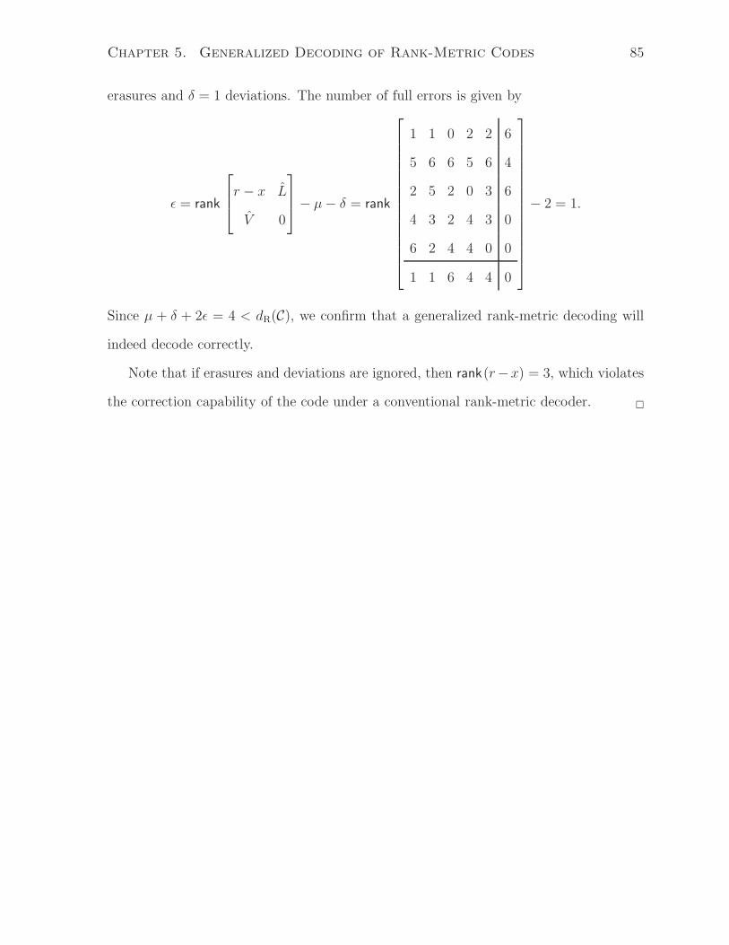
Chapter 5. Generalized Decoding of Rank-Metric Codes 85
erasures and δ = 1 deviations. The number of full errors is given by
ǫ = rank
r − x L
V 0
− µ − δ = rank
1 1 0 2 2 6
5 6 6 5 6 4
2 5 2 0 3 6
4 3 2 4 3 0
6 2 4 4 0 0
1 1 6 4 4 0
− 2 = 1.
Since µ + δ + 2ǫ = 4 < dR(C), we confirm that a generalized rank-metric decoding will
indeed decode correctly.
Note that if erasures and deviations are ignored, then rank(r−x) = 3, which violates
the correction capability of the code under a conventional rank-metric decoder.
Chapter 6
Efficient Encoding and Decoding of
Gabidulin Codes
The goal of this chapter is to propose a computationally efficient algorithm for solving
the generalized rank-metric decoding problem (with errors, erasures and deviations) up
to the errata correction capability of the code. Our algorithm is applicable to Gabidulin
codes.
More precisely, we show in Section 6.2 how to modify the standard decoding algorithm
for Gabidulin codes (reviewed in Section 6.1) in order to incorporate erasures and devia-
tions. No significant increase of complexity is observed with this modification. Moreover,
in Section 6.3 we propose the use of optimal (or low-complexity) normal bases to signifi-
cantly speed up the algorithm. In addition, in Section 6.4, we propose a novel algorithm
based on transform-domain approach. Such a transform-domain approach was origi-
nally proposed by Blahut for Reed-Solomon codes [59, 60]; here, we adapt it Gabidulin
codes, which requires new results and interpretations regarding linearized polynomials.
Additional contributions of this chapter are two new encoding algorithms for Gabidulin
codes, which are described in Section 6.5. Together, our proposed encoding and decoding
algorithms appear to be the fastest know to date.
86
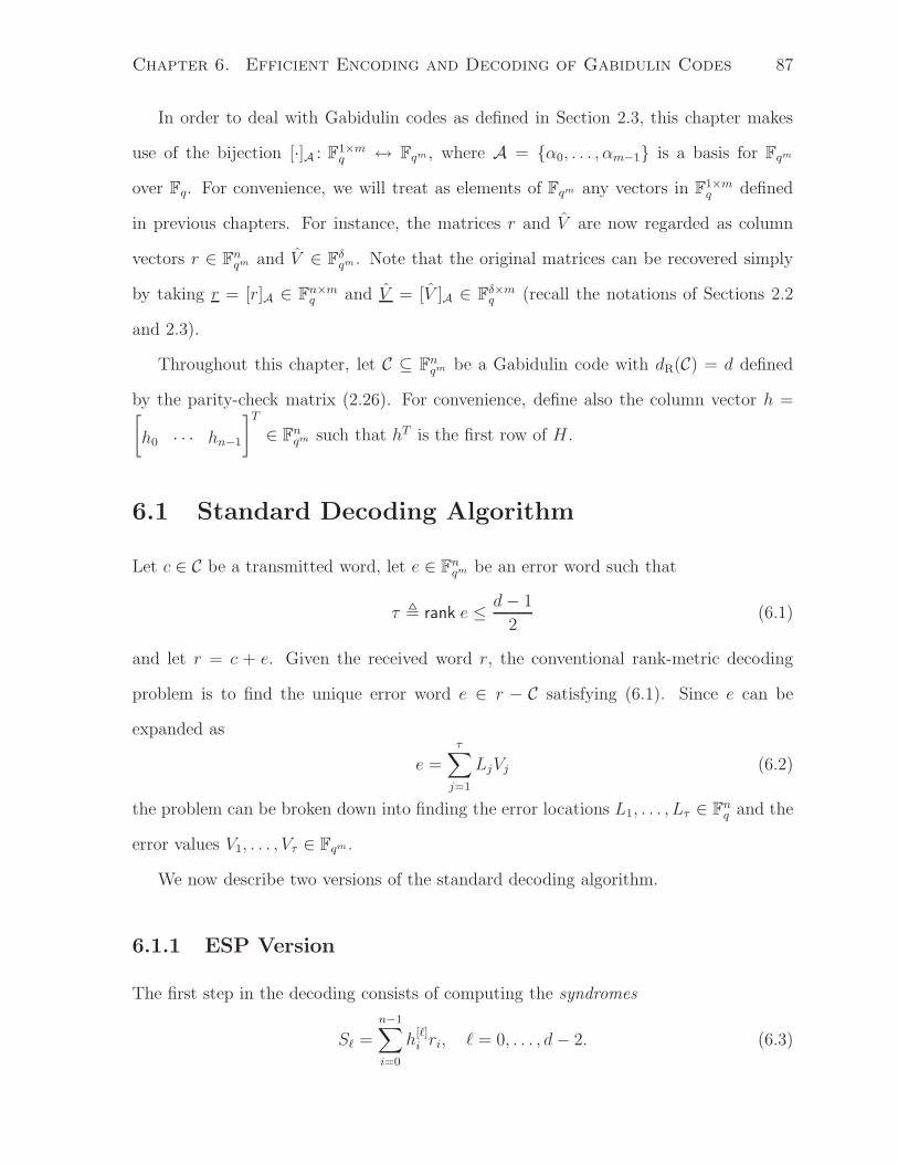
Chapter 6. Efficient Encoding and Decoding of Gabidulin Codes 87
In order to deal with Gabidulin codes as defined in Section 2.3, this chapter makes
use of the bijection [·]A : F1×mq ↔ Fqm , where A = α0, . . . , αm−1 is a basis for Fqm
over Fq. For convenience, we will treat as elements of Fqm any vectors in F1×mq defined
in previous chapters. For instance, the matrices r and V are now regarded as column
vectors r ∈ Fnqm and V ∈ Fδ
qm. Note that the original matrices can be recovered simply
by taking r = [r]A ∈ Fn×mq and V = [V ]A ∈ Fδ×m
q (recall the notations of Sections 2.2
and 2.3).
Throughout this chapter, let C ⊆ Fnqm be a Gabidulin code with dR(C) = d defined
by the parity-check matrix (2.26). For convenience, define also the column vector h =[
h0 · · · hn−1
]T
∈ Fnqm such that hT is the first row of H .
6.1 Standard Decoding Algorithm
Let c ∈ C be a transmitted word, let e ∈ Fnqm be an error word such that
τ , rank e ≤ d − 1
2(6.1)
and let r = c + e. Given the received word r, the conventional rank-metric decoding
problem is to find the unique error word e ∈ r − C satisfying (6.1). Since e can be
expanded as
e =τ∑
j=1
LjVj (6.2)
the problem can be broken down into finding the error locations L1, . . . , Lτ ∈ Fnq and the
error values V1, . . . , Vτ ∈ Fqm.
We now describe two versions of the standard decoding algorithm.
6.1.1 ESP Version
The first step in the decoding consists of computing the syndromes
Sℓ =
n−1∑
i=0
h[ℓ]i ri, ℓ = 0, . . . , d − 2. (6.3)
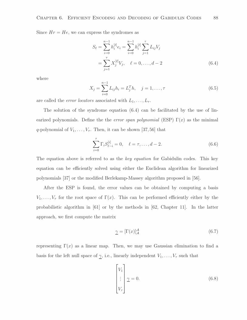
Chapter 6. Efficient Encoding and Decoding of Gabidulin Codes 88
Since Hr = He, we can express the syndromes as
Sℓ =
n−1∑
i=0
h[ℓ]i ei =
n−1∑
i=0
h[ℓ]i
τ∑
j=1
LijVj
=
τ∑
j=1
X[ℓ]j Vj , ℓ = 0, . . . , d − 2 (6.4)
where
Xj =n−1∑
i=0
Lijhi = LTj h, j = 1, . . . , τ (6.5)
are called the error locators associated with L1, . . . , Lτ .
The solution of the syndrome equation (6.4) can be facilitated by the use of lin-
earized polynomials. Define the the error span polynomial (ESP) Γ(x) as the minimal
q-polynomial of V1, . . . , Vτ . Then, it can be shown [37, 56] that
τ∑
i=0
ΓiS[i]ℓ−i = 0, ℓ = τ, . . . , d − 2. (6.6)
The equation above is referred to as the key equation for Gabidulin codes. This key
equation can be efficiently solved using either the Euclidean algorithm for linearized
polynomials [37] or the modified Berlekamp-Massey algorithm proposed in [56].
After the ESP is found, the error values can be obtained by computing a basis
V1, . . . , Vτ for the root space of Γ(x). This can be performed efficiently either by the
probabilistic algorithm in [61] or by the methods in [62, Chapter 11]. In the latter
approach, we first compute the matrix
γ = [Γ(x)]AA (6.7)
representing Γ(x) as a linear map. Then, we may use Gaussian elimination to find a
basis for the left null space of γ, i.e., linearly independent V1, . . . , Vτ such that
V1
...
Vτ
γ = 0. (6.8)

Chapter 6. Efficient Encoding and Decoding of Gabidulin Codes 89
To find the error locators, one can use Gabidulin’s algorithm [37, pp. 9–10], which is
an efficient algorithm to solve a system of the form (6.4).
After X1, . . . , Xτ and V1, . . . , Vτ are found, the error locations can be computed by
inverting (6.5), i.e., by
LTj = Xj(h)†, (6.9)
where (h)† is a right-inverse of h. Note that (h)† can be precomputed. Finally, the error
word is computed from (6.2).
6.1.2 ELP Version
Due to the similarity between error locators and error values, an alternative approach
exists where the error locators are computed before the error values.
First, compute the “reversed syndromes”
Sℓ , S[ℓ−d+2]d−2−ℓ =
τ∑
j=1
V[ℓ−d+2]j Xj , ℓ = 0, . . . , d − 2. (6.10)
Note that (6.10) has the same form as (6.4), with the roles of Vj and Xj exchanged.
Define the error locator polynomial (ELP) Λ(x) as the minimal q-polynomial of
X1, . . . , Xτ . Then, it can be shown [57] that
τ∑
i=0
ΛiS[i]ℓ−i = 0, ℓ = τ, . . . , d − 2. (6.11)
This key equation has the same form as (6.8) and can be solved by exactly the same
methods.
After the ELP is found, we can use exactly the same procedure outlined in Sec-
tion 6.1.1 to find a basis X1, . . . , Xτ for the root space of Λ(x); namely, we first compute
λ = [Λ(x)]AA (6.12)

Chapter 6. Efficient Encoding and Decoding of Gabidulin Codes 90
and then solve
X1
...
Xτ
λ = 0. (6.13)
Then, as before, Gabidulin’s algorithm may be used to solve (6.10) and find the error
values.
The remainder of the algorithm is identical to that of Section 6.1.1.
6.1.3 Summary and Complexity
A summary of the algorithm is given below. The algorithm consists of six steps:
1) Find the syndromes: Compute (6.3);
2) Find the ESP/ELP: Solve (6.6)/(6.11) using the Berlekamp-Massey algorithm [56];
3) Find a basis for the root space of the ESP/ELP:
a) Compute (6.7)/(6.12);
b) Solve (6.8)/(6.13) using Gaussian elimination;
4) Find the error locators/error values: Solve (6.4)/(6.10) using Gabidulin’s algo-
rithm [37];
5) Find the error locations: Compute (6.9);
6) Find the error word: Compute (6.2).
A breakdown of complexity is given in Table 6.1. The complexity of Step 3a corre-
sponds to m evaluations of a linearized polynomial (with lowest-order coefficient equal
to 1) of q-degree τ (see Section 2.4), while the complexity of Step 3b corresponds to con-
verting an m×m matrix of rank m−τ to reduced column-echelon form (see Section 2.1).
The complexity of the remaining steps is taken from [63]. It can be seen that the overall
complexity is dominated by Steps 1 and 3a, each requiring O(dm3) operations in Fq.
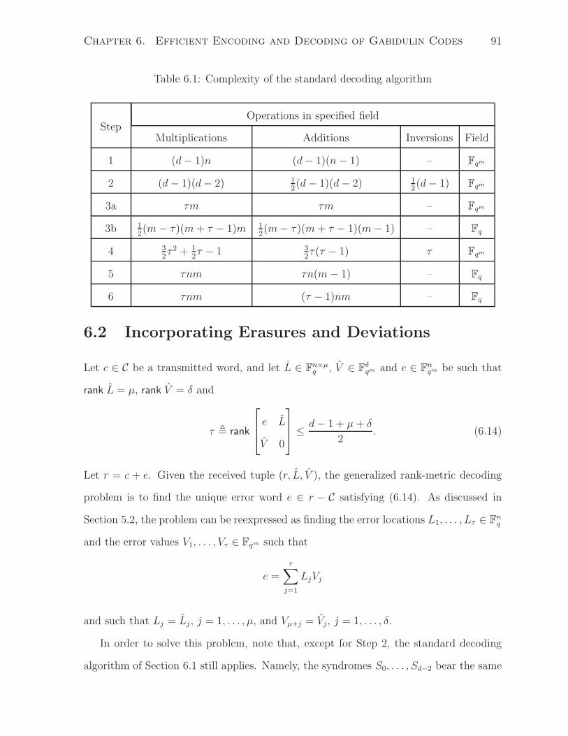
Chapter 6. Efficient Encoding and Decoding of Gabidulin Codes 91
Table 6.1: Complexity of the standard decoding algorithm
StepOperations in specified field
Multiplications Additions Inversions Field
1 (d − 1)n (d − 1)(n − 1) – Fqm
2 (d − 1)(d − 2) 12(d − 1)(d − 2) 1
2(d − 1) Fqm
3a τm τm – Fqm
3b 12(m − τ)(m + τ − 1)m 1
2(m − τ)(m + τ − 1)(m − 1) – Fq
4 32τ 2 + 1
2τ − 1 3
2τ(τ − 1) τ Fqm
5 τnm τn(m − 1) – Fq
6 τnm (τ − 1)nm – Fq
6.2 Incorporating Erasures and Deviations
Let c ∈ C be a transmitted word, and let L ∈ Fn×µq , V ∈ Fδ
qm and e ∈ Fnqm be such that
rank L = µ, rank V = δ and
τ , rank
e L
V 0
≤ d − 1 + µ + δ
2. (6.14)
Let r = c + e. Given the received tuple (r, L, V ), the generalized rank-metric decoding
problem is to find the unique error word e ∈ r − C satisfying (6.14). As discussed in
Section 5.2, the problem can be reexpressed as finding the error locations L1, . . . , Lτ ∈ Fnq
and the error values V1, . . . , Vτ ∈ Fqm such that
e =τ∑
j=1
LjVj
and such that Lj = Lj , j = 1, . . . , µ, and Vµ+j = Vj, j = 1, . . . , δ.
In order to solve this problem, note that, except for Step 2, the standard decoding
algorithm of Section 6.1 still applies. Namely, the syndromes S0, . . . , Sd−2 bear the same

Chapter 6. Efficient Encoding and Decoding of Gabidulin Codes 92
relationship (6.4) to the error locators X1, . . . , Xµ and the error values V1, . . . , Vδ (or
(6.10) for the reversed syndromes). Moreover, if either the ESP or the ELP is found,
then the algorithm can be resumed at Step 3 and carried out unchanged. (This is because
(6.14) implies µ + δ ≤ (d − 1)/2 and therefore τ ≤ d − 1, which is the only assumption
needed at Step 4.) Thus, only Step 2 needs to be modified in order to incorporate erasures
and deviations.
In the following, we present such modification for both the ESP version and ELP
version of the algorithm. In both cases, the decoder computes
Xj = LTj h, j = 1, . . . , µ (6.16)
ΛU(x) = MX1,...,Xµ(x) (6.17)
ΓD(x) = MV1,...,Vδ(x). (6.18)
Let S(x) =∑d−2
ℓ=0 Sℓx[ℓ] be the syndrome polynomial and let S(x) be the partial q-
reverse of S(x). Also, let ΛU(x) and ΓD(x) be the partial q-reverses of ΛU(x) and ΓD(x),
respectively. Let ǫ = τ − µ − δ.
6.2.1 ESP Version
Let ΓF (x) and ΓU(x) be the minimal linearized polynomials satisfying
ΓF (ΓD(Vj)) = 0, j = µ + δ + 1, . . . , τ
ΓU(ΓF (ΓD(Vj))) = 0, j = 1, . . . , µ.
Since Vµ+1, . . . , Vτ are necessarily linearly independent, we have that the q-degrees of
ΓD(x) and ΓF (x) ⊗ ΓD(x) are δ and δ + ǫ, respectively, and therefore the q-degree of
ΓF (x) must be ǫ. On the other hand, all the Vj may not be linearly independent, so the
q-degree of ΓU(x) is at most µ. It follows that the error span polynomial is given by
Γ(x) = ΓU(x) ⊗ ΓF (x) ⊗ ΓD(x) (6.19)

Chapter 6. Efficient Encoding and Decoding of Gabidulin Codes 93
and it has q-degree at most τ . Since ΓD(x) is known to the decoder, finding Γ(x) reduces
to the determination of ΓF (x) and ΓU(x).
We define an auxiliary syndrome polynomial as
SDU(x) = ΓD(x) ⊗ S(x) ⊗ ΛU(x). (6.20)
Observe that SDU(x) incorporates all the information that is known at the decoder,
including erasures and deviations.
Our modified key equation is given in the following theorem.
Theorem 6.1:
ΓF (x) ⊗ SDU(x) ≡ Ω(x) mod x[d−1]
where Ω(x) is a linearized polynomial of q-degree ≤ τ − 1. Equivalently, we may write
ǫ∑
i=0
ΓF,iS[i]DU,µ+δ+ℓ−i = 0, ℓ = ǫ, . . . , d − 2 − µ − δ. (6.22)
Proof: Let Ω(x) = ΓF (x) ⊗ SDU(x) mod x[d−1]. If τ ≥ d − 1, we have nothing to prove,
so let us assume τ ≤ d − 2. We will show that Ωℓ = 0 for ℓ = τ, . . . , d − 2.
Let ΓFD(x) = ΓF (x) ⊗ ΓD(x) and
SFD(x) = ΓF (x) ⊗ ΓD(x) ⊗ S(x) = ΓFD(x) ⊗ S(x). (6.23)
According to (2.30), for ǫ + δ ≤ ℓ ≤ d − 2 we have
SFD,ℓ =
ǫ+δ∑
i=0
ΓFD,iS[i]ℓ−i =
ǫ+δ∑
i=0
ΓFD,i
(τ∑
j=1
X[ℓ−i]j Vj
)[i]
=τ∑
j=1
X[ℓ]j ΓFD(Vj) =
µ∑
j=1
X[ℓ]j ζj, (6.24)
where
ζj = ΓFD(Vj), j = 1, . . . , µ.

Chapter 6. Efficient Encoding and Decoding of Gabidulin Codes 94
Note that ΓF (x)⊗SDU (x) = SFD(x)⊗ ΛU (x). Using (2.31) and (6.24), for µ+ ǫ+δ ≤
ℓ ≤ d − 2 we have
Ωℓ =
µ∑
i=0
Λ[ℓ−i]U,i SFD,ℓ−i =
µ∑
i=0
Λ[ℓ−µ]U,µ−i
µ∑
j=1
X[ℓ−i]j ζj
=
µ∑
j=1
µ∑
i=0
Λ[ℓ−µ]U,i X
[ℓ−µ+i]j ζj =
µ∑
j=1
ΛU(Xj)[ℓ−µ]ζj = 0.
This completes the proof of the theorem.
Note that this key equation reduces to the original key equation (6.6) when there are
no erasures or deviations. Moreover, it can be solved by the same methods as the original
key equation (6.6), e.g., using the Euclidean algorithm for linearized polynomials [37] or
using the modified Berlekamp-Massey algorithm from [56], provided 2ǫ ≤ d − 1 − µ − δ
(which is true by assumption). Note that we should take “Sℓ” in (6.6) as SDU,ℓ+µ+δ and
take “d” as d − µ − δ.
After computing ΓF (x), we still need to determine ΓU(x). In the proof of Theorem 6.1,
observe that (6.24) has the same form as (6.4); thus, ζ1, . . . , ζµ can be computed using
Gabidulin’s algorithm [37], since SFD(x) and X1, . . . , Xµ are known. Finally, ΓU(x) can
be obtained as the minimal q-polynomial of ζ1, . . . , ζµ, i.e.,
ΓU(x) = Mζ1,...,ζµ(x). (6.26)
6.2.2 ELP Version
Let ΛF (x) and ΛD(x) be the minimal linearized polynomials satisfying
ΛF (ΛU(Xj)) = 0, j = µ + δ + 1, . . . , τ
ΛD(ΛF (ΛU(Xj))) = 0, j = µ + 1, . . . , µ + δ.
As before, we have that the q-degree of ΛF (x) is ǫ and the q-degree of ΛD(x) is at most
δ. The error locator polynomial is given by
Λ(x) = ΛD(x) ⊗ ΛF (x) ⊗ ΛU(x) (6.27)

Chapter 6. Efficient Encoding and Decoding of Gabidulin Codes 95
and it has q-degree at most τ . Since ΛU(x) is known to the decoder, we only need to
determine ΛF (x) and ΛD(x).
Let the auxiliary syndrome polynomial be defined as
SUD(x) = ΛU(x) ⊗ S(x) ⊗ ΓD(x[d−2])[−d+2]. (6.28)
We have the following key equation:
Theorem 6.2:
ΛF (x) ⊗ SUD(x) ≡ Ψ(x) mod x[d−1]
where Ψ(x) is a linearized polynomial of q-degree ≤ τ − 1. Equivalently, we may write
ǫ∑
i=0
ΛF,iS[i]UD,µ+δ+ℓ−i = 0, ℓ = ǫ, . . . , d − 2 − µ − δ. (6.30)
Proof: Let Ψ(x) = ΛF (x) ⊗ SUD(x) mod x[d−1]. We will show that Ψℓ = 0 for ℓ =
τ, . . . , d − 2.
Let ΛFU(x) = ΛF (x) ⊗ ΛU(x) and
SFU(x) = ΛF (x) ⊗ ΛU(x) ⊗ S(x) = ΛFU(x) ⊗ S(x). (6.31)
According to (2.30), for ǫ + µ ≤ ℓ ≤ d − 2 we have
SFU,ℓ =
ǫ+µ∑
i=0
ΛFU,iS[i]ℓ−i =
ǫ+µ∑
i=0
ΛFU,i
(τ∑
j=1
V[ℓ−i−d+2]j Xj
)[i]
=
τ∑
j=1
V[ℓ−d+2]j ΛFU(Xj) =
δ∑
j=1
V[ℓ−d+2]µ+j ξj, (6.32)
where ξj = ΛFU(Xµ+j), j = 1, . . . , δ.
Note that ΛF (x) ⊗ SUD(x) = SFU(x) ⊗ ΓD(x[d−2])[−d+2]
. Using (2.31) and (6.32), for

Chapter 6. Efficient Encoding and Decoding of Gabidulin Codes 96
δ + ǫ + µ ≤ ℓ ≤ d − 2 we have
Ψℓ =
δ∑
i=0
(Γ[−d+2]D,i )
[ℓ−i]SFU,ℓ−i
=δ∑
i=0
Γ[ℓ−δ−d+2]D,δ−i
δ∑
j=1
V[ℓ−i−d+2]µ+j ξj
=δ∑
j=1
δ∑
i=0
Γ[ℓ−δ−d+2]D,i V
[ℓ−δ+i−d+2]µ+j ξj
=δ∑
j=1
ΓD(Vµ+j)[ℓ−δ−d+2]ξj = 0.
This completes the proof of the theorem.
After computing ΛF (x), we can determine ΛD(x) in the following way. First, we apply
Gabidulin’s algorithm on (6.32) in order to obtain ξ1, . . . , ξδ. Then, we compute ΛD(x)
as the minimal q-polynomial of ξ1, . . . , ξδ, i.e.,
ΛD(x) = Mξ1,...,ξδ(x). (6.33)
6.2.3 Summary and Complexity
A summary of the modified Step 2 is given below. It consists of nine sub-steps:
2) Find the ESP/ELP:
a) Compute (6.16);
b) Compute (6.17);
c) Compute (6.18);
d) Compute (6.20)/(6.28);
e) Solve (6.22)/(6.30) using the Berlekamp-Massey algorithm [56];
f) Compute (6.23)/(6.31);
g) Solve (6.24)/(6.32) using Gabidulin’s algorithm [37];

Chapter 6. Efficient Encoding and Decoding of Gabidulin Codes 97
Table 6.2: Complexity of modified Step 2 to incorporate erasures and deviations. Short-
hand: d′ = d − µ − δ.
StepOperations in specified field
Multiplications Additions Inversions Field
2a µnm µ(n − 1)m – Fq
2b µ2 µ(µ − 1) µ Fqm
2c δ2 δ(δ − 1) δ Fqm
2d (d − 1)(µ + δ) + µδ (d − 2)(µ + δ) + µδ – Fqm
2e (d′ − 1)(d′ − 2) 12(d′ − 1)(d′ − 2) 1
2(d′ − 1) Fqm
2f (ESP) ǫ(d − 1 + δ) ǫ(d − 2 + δ) – Fqm
2g (ESP) 32µ2 + 1
2µ − 1 3
2µ(µ − 1) µ Fqm
2h (ESP) µ2 µ(µ − 1) µ Fqm
2f (ELP) ǫ(d − 1 + µ) ǫ(d − 2 + µ) – Fqm
2g (ELP) 32δ2 + 1
2δ − 1 3
2δ(δ − 1) δ Fqm
2h (ELP) δ2 δ(δ − 1) δ Fqm
2i ǫ(µ + δ) + µδ ǫ(µ + δ) + µδ – Fqm
h) Compute (6.26)/(6.33);
i) Compute (6.19)/(6.27).
The complexity of each sub-step is given in Table 6.2. A few comments are in order. The
complexity of Steps 2a–2e and 2i do not vary between the ESP and the ELP versions.
In Step 2f, a few operations are avoided since we can reuse the product ΓD(x)⊗S(x) (or
ΛU(x)⊗ S(x)) computed in Step 2d. In the ESP version, Steps 2a, 2b, 2f, 2g and 2h can
be skipped if there are no erasures. Similarly, in the ELP version, Steps 2c, 2f, 2g and
2h can be skipped if there are no deviations.

Chapter 6. Efficient Encoding and Decoding of Gabidulin Codes 98
Assuming that the decoder can freely choose between the ESP version and the ELP
version depending on the values µ and δ, the worst-case complexity is obtained in the
case where µ = δ = (d − 1)/2 (assuming for simplicity that d is odd). In this case, the
complexity of Step 2 is given by
21
8(d − 1)2 +
1
4(d − 1) − 1 multiplications in Fqm
21
8(d − 1)2 − 13
4(d − 1) additions in Fqm
2(d − 1) inversions in Fqm
where we have ignored the Fq-operations in Step 2a. By comparing with Table 6.1, we
can see that the complexity of Step 2 with erasures and deviations is at most 7 times
the complexity of this step when only errors occur. Thus, incorporating erasures and
deviations does not increase the order of complexity of the decoding algorithm.
6.3 Fast Decoding Using Low-Complexity Normal
Bases
In this section, we describe how the decoding algorithm of the previous sections can be
made much more efficient.
We assume that A = α[i] is a low-complexity normal basis with multiplication table
T , and that Fq has characteristic 2. The essence of our approach lies in the following
expression:
aα[i] =(a←iT
)→i, ∀i = 0, . . . , m − 1.
In other words, multiplying an element of Fqm by a q-power of α costs only C(T )−m
additions in Fq (recall that T lies in F2), rather than O(m2) operations in Fq as in a
general multiplication.

Chapter 6. Efficient Encoding and Decoding of Gabidulin Codes 99
Let H ′ =
[
α[i+j]
]
, 0 ≤ i ≤ d− 2, 0 ≤ j ≤ n′ − 1. Then H = H ′A for some A ∈ Fn′×nq
and some n ≤ n′ ≤ m. Thus, the map given by c′ = Ac is an injection from C to C′,
where C′ ∈ Fn′
qm is the Gabidulin code defined by H ′. Note that dR(C′) = d. Thus, a
tuple (r, L, E) can be decoded by first applying a decoder for C′ on the tuple (Ar, AL, E),
yielding a codeword c′ = Ac, and then computing c = A†c′, where A† is a left inverse of
A. The decoding complexity is equal to n′n(2m + µ) additions and multiplications in Fq
plus the complexity of decoding C′. Thus, we will assume in the following that hi = α[i],
i = 0, . . . , n − 1. (Note that there is apparently no good reason for choosing a different
H .)
Now, consider the syndrome computation in Step 1. We have
Sℓ =n−1∑
i=0
riα[i+ℓ], ℓ = 0, . . . , d − 2. (6.35)
It follows that the syndromes can be computed with only (d − 1)n(C(T ) − m) + (d −
1)(n − 1)m = (d − 1)(nC(T ) − m) additions in Fq (no multiplications).
Consider the computation of
γj = Γ(α[j]) =
τ∑
i=0
Γiα[i+j], j = 0, . . . , m − 1 (6.36)
or
λj = Λ(α[j]) =
τ∑
i=0
Λiα[i+j], j = 0, . . . , m − 1 (6.37)
in Step 3a. Either computation can be done simply with τm(C(T )−m)+τm2 = τmC(T )
additions in Fq.
Thus, the steps that were once the most demanding ones are now among the easiest
to perform.
There are some additional savings. Note that h is now an identity matrix with m−n
additional all-zero columns at the right; thus the cost of computing Lj from Xj in Step 5
reduces to zero. (In particular, if n = m, then Xj = LTj , i.e., LT
j is precisely the vector
representation of Xj with respect to the normal basis.)

Chapter 6. Efficient Encoding and Decoding of Gabidulin Codes 100
Table 6.3: Complexity of the updated decoding steps for a code matched to a normal
basis of complexity C(T ) over a field of characteristic 2.
StepOperations in specified field
Multiplications Additions Inversions Field
1 – (d − 1)(nC(T ) − m) – Fq
3a – τmC(T ) – Fq
5 – – – Fq
The complexity of the updated steps is shown in Table 6.3. It follows that the decoding
complexity is now dominated by Steps 2 and 4 (although the kernel computation in
Step 3b may become significant if d is very small). For n = m and d = 2τ + 1, the
overall complexity of the algorithm is approximately 112τ 2m2 + 1
2m3 multiplications and
112τ 2mC(T )+ 1
2m3 additions in Fq. An example is illustrated in Fig. 6.1 for varying rates.
6.4 Transform-Domain Methods
6.4.1 Linear Maps over Fqm and the q-Transform
In this section, unless otherwise mentioned, all polynomials are q-polynomials over Fqm
with q-degree smaller than m. If v ∈ Fnqm is a vector of length n ≤ m over Fqm, we will
take v to have length m, i.e., v ∈ Fmqm, and set vn = · · · = vm−1 = 0.
We adopt the following convenient notation: if f(x) =∑
i=0 fix[i] is q-polynomial,
then f =
[
f0 · · · fm−1
]T
is a vector over Fqm, and vice-versa. Thus, f(x) and f are
simply equivalent representations for the sequence f0, . . . , fm−1. In addition, we adopt a
cyclic indexing for any such a sequence: namely, we define fi = fi mod m for all i. With
this notation, we can write the symbolic multiplication h(x) = f(x)⊗ g(x) mod x[m] − x
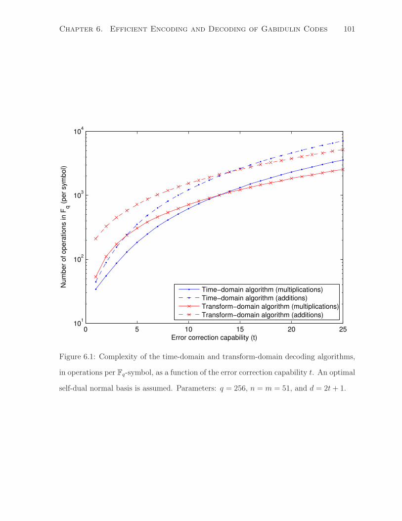
Chapter 6. Efficient Encoding and Decoding of Gabidulin Codes 101
0 5 10 15 20 2510
1
102
103
104
Error correction capability (t)
Nu
mb
er
of
op
era
tio
ns in
Fq (
pe
r sym
bo
l)
Time−domain algorithm (multiplications)
Time−domain algorithm (additions)
Transform−domain algorithm (multiplications)
Transform−domain algorithm (additions)
Figure 6.1: Complexity of the time-domain and transform-domain decoding algorithms,
in operations per Fq-symbol, as a function of the error correction capability t. An optimal
self-dual normal basis is assumed. Parameters: q = 256, n = m = 51, and d = 2t + 1.

Chapter 6. Efficient Encoding and Decoding of Gabidulin Codes 102
as a cyclic “q-convolution,” namely,
hℓ =m−1∑
i=0
fig[i]ℓ−i =
m−1∑
j=0
fℓ−jg[ℓ−j]j , ℓ = 0, . . . , m − 1. (6.38)
Recall that the full q-reverse of a q-polynomial f(x) is the q-polynomial f(x) =
∑m−1i=0 fix
[i], where fi = f[i]−i, ∀i.
For the remainder of this subsection, A = αi, B = βi and Θ = θi are bases for
Fqm over Fq, with dual bases A′ = α′i, B′ = β ′i and Θ′ = θ′i, respectively.
Lemma 6.3: M =
[
f(x)
]B
A
⇐⇒ MT =
[
f(x)
]A′
B′.
Proof: By (2.16), we have
f(αi) =
m−1∑
j=0
Mijβj.
This implies that, for all i, j,
Mij = Tr(f(αi)β
′j
)
=
m−1∑
ℓ=0
Tr(
fℓα[ℓ]i β ′j
)
=
m−1∑
ℓ=0
Tr(
f−ℓα[−ℓ]i β ′j
)
=
m−1∑
ℓ=0
Tr(
f[ℓ]−ℓαiβ
′j[ℓ])
(6.40)
= Tr
(m−1∑
ℓ=0
fℓβ′j[ℓ]
αi
)
= Tr(f(β ′j)αi
)
where (6.40) follows from (2.20).
Now, let N =
[
f(x)
]A′
B′. From (2.16) we have
f(β ′j) =m−1∑
k=0
Njkα′k

Chapter 6. Efficient Encoding and Decoding of Gabidulin Codes 103
which implies that, for all i, j,
Nji = Tr(f(β ′j)αi
)= Mij .
Thus, N = MT . The converse part follows immediately from the fact that ¯f(x) = f(x).
Lemma 6.4: Suppose A is a normal basis. Let F ∈ Fmqm be such that
[
F
]
B
=
[
f(x)
]B
A
.
Then fi = F (α′i), i = 0, . . . , m − 1. In particular,
[
f
]
Θ
=
[
F (x)
]Θ
A′
.
Proof: By (2.16), we have
Fj = f(α[j]), j = 0, . . . , m − 1.
It follows that, for all i,
F (α′[i]
) =m−1∑
j=0
Fjα′[i+j]
=m−1∑
j=0
f(α[j])α′[i+j]
=
m−1∑
j=0
m−1∑
ℓ=0
fℓα[ℓ+j]α′
[i+j]
=m−1∑
ℓ=0
fℓ Tr(
α[ℓ]α′[i])
= fi.
Definition 6.1: The q-transform of a vector f ∈ Fmqm (or a q-polynomial f(x)) with
respect to a normal element α is the vector F ∈ Fmqm (or the q-polynomial F (x)) given
by Fj = f(α[j]) =∑m−1
i=0 fiα[i+j], j = 0, . . . , m − 1.
Theorem 6.5: The inverse q-transform of a vector F ∈ Fmqm (or a q-polynomial F (x))
with respect to α is given by fi = F (α′[i]) =∑m−1
j=0 Fjα[i+j], i = 0, . . . , m − 1. In other
words, the inverse q-transform with respect to α is equal to the forward q-transform with
respect to α′.
Proof: Follows immediately from Lemma 6.4 by taking B = Θ to be the basis for Fqm .

Chapter 6. Efficient Encoding and Decoding of Gabidulin Codes 104
6.4.2 Implications to the Decoding of Gabidulin Codes
Recall the notations of Section 6.1. Assume that A = α[i] is a normal basis and that
the Gabidulin code has parity-check matrix H =
[
α[i+j]
]
.
As in the transform-domain decoding of Reed-Solomon codes [60], the equation r =
c+e, or r(x) = c(x)+e(x), is translated to the transform domain as R(x) = C(x)+E(x),
where R(x), C(x) and E(x) are the q-transforms with respect to α of r(x), c(x) and
e(x), respectively. Now, the fact that Cℓ = c(α[ℓ]) = 0, ℓ = 0, . . . , d − 2, implies that
Sℓ = Rℓ = Eℓ, ℓ = 0, . . . , d − 2. Note also that Sℓ = Eℓ−d+2, ℓ = 0, . . . , d − 2.
Lemma 6.6: Let A(x), B(x) and E(x) be linearized polynomials with q-degrees at most
a, b and m − 1, respectively. Let S(x) be another linearized polynomial, and suppose
that E(x) and S(x) agree in the coefficients ℓ = 0, . . . , d − 2. Then A(x) ⊗ E(x) ⊗
B(x) mod x[m] − x and A(x)⊗ S(x)⊗B(x) agree in the coefficients ℓ = a + b, . . . , d− 2.
Proof: Let P (x) = A(x)⊗E(x) mod x[m] − x and let Q(x) = A(x)⊗ S(x). From (6.38)
and (2.30), we have that, for ℓ = a, . . . , d − 2,
Pℓ =
a∑
i=0
AiE[i]ℓ−i =
a∑
i=0
AiS[i]ℓ−i = Qℓ.
Now, let Ψ(x) = P (x) ⊗ B(x) mod x[m] − x and let Ω(x) = Q(x) ⊗ B(x). From (6.38)
and (2.30), we have that, for ℓ = a + b, . . . , d − 2,
Ψℓ =b∑
j=0
Eℓ−jB[ℓ−j]j =
b∑
j=0
Sℓ−jB[ℓ−j]j = Ωℓ.
Theorem 6.7 (The Key Equations):
Γ(x) ⊗ E(x) ≡ 0 (mod x[m] − x) (6.45)
Λ(x) ⊗ E(x) ≡ 0 (mod x[m] − x). (6.46)
In particular, (6.6) and (6.11) hold.

Chapter 6. Efficient Encoding and Decoding of Gabidulin Codes 105
Proof: For the first key equation, let γ =
[
Γ(x)
]A
A
. Note that Γ(Vj) = 0 implies Vj γ = 0,
j = 1, . . . , τ . From (2.18) we have
[
Γ(x) ⊗ E(x)
]A
A′
=
[
E(x)
]A
A′
[
Γ(x)
]A
A
= e γ =τ∑
j=1
XjT Vj γ = 0.
Thus, we obtain (6.45). The form (6.6) of this key equation follows immediately after
applying Lemma 6.6.
For the second key equation, let λ =
[
Λ(x)
]A
A
. Note that Λ(Xj) = 0 implies Xj λ = 0,
j = 1, . . . , τ . From (2.18) we have
[
Λ(x) ⊗ E(x)
]A
A′
=
[
E(x)
]A
A′
[
Γ(x)
]A
A
= eT λ =τ∑
j=1
VjT Xj λ = 0.
To obtain the form (6.11), we first have to multiply both sides of (6.46) on the right by
x[d−2] (so that E(x) ⊗ x[d−2] agrees with S(x)), and then apply Lemma 6.6.
Theorem 6.8 (The Modified Key Equations):
ΓF (x) ⊗ ΓD(x) ⊗ E(x) ⊗ ΛU(x) ≡ 0 (mod x[m] − x) (6.49)
ΛF (x) ⊗ ΛU(x) ⊗ E(x) ⊗ ΓD(x) ≡ 0 (mod x[m] − x). (6.50)
In particular, (6.22) and (6.30) hold.
Proof: For the first key equation, let ΓFD(x) = ΓF (x) ⊗ ΓD(x) and γFD =
[
ΓFD(x)
]A
A
.
Note that ΓFD(Vj) = 0 implies Vj γFD = 0, j = µ+1, . . . , τ . Similarly, let λU =
[
ΛU(x)
]A
A
and note that Xj λU = 0, j = 1, . . . , µ. From (2.18) we have
[
ΓFD(x) ⊗ E(x) ⊗ ΛU(x)
]A
A′
=
[
ΛU(x)
]A′
A′
[
E(x)
]A
A′
[
ΓFD(x)
]A
A
= λUT e γFD
=
τ∑
j=1
λUT Xj
T Vj γFD = 0.

Chapter 6. Efficient Encoding and Decoding of Gabidulin Codes 106
For the second key equation, let ΛFU(x) = ΛF (x) ⊗ ΛU(x) and λFU =
[
ΛFU(x)
]A
A
.
Note that ΛFU(Xj) = 0 implies Xj λFU = 0, j = 1, . . . , µ, µ + δ + 1, . . . , τ . Similarly, let
γD =
[
ΓD(x)
]A
A
and note that Vj γD = 0, j = µ + 1, . . . , µ + δ. From (2.18) we have
[
ΛFU(x) ⊗ E(x) ⊗ ΓD(x)
]A
A′
=
[
ΓD(x)
]A′
A′
[
E(x)
]A
A′
[
ΛFU(x)
]A
A
= γDT eT λFU
=
τ∑
j=1
γDT Vj
T Xj λFU = 0.
The alternative forms (6.22) and (6.30) follow after applying Lemma 6.6 and per-
forming a few manipulations. In particular, (6.30) follows by applying Lemma 6.6 on
(ΛF (x) ⊗ ΛU(x)) ⊗(E(x) ⊗ x[d−2]
)⊗(x[−d+2] ⊗ ΓD(x) ⊗ x[d−2]
)mod x[m] − x.
Besides allowing us to give conceptually simpler proofs of the key equations, the
transform approach also provides us with the theoretical ground for proposing a new
decoding algorithm for Gabidulin codes. The main idea is that, after the ESP or the
ELP is found, the remaining coefficients of E(x) can be computed using the recursion
Eℓ = −τ∑
i=1
ΓiE[i]ℓ−i = 0, ℓ = d − 1, . . . , m − 1 (6.51)
Eℓ = −τ∑
i=0
ΛiE[i]ℓ−i = 0, ℓ = 1, . . . , m − d + 1. (6.52)
Then, the error polynomial e(x) can be obtained through an inverse q-transform, i.e.,
ei = E(α′[i]
) =m−1∑
j=0
ejα′[i+j]
, i = 0, . . . , n − 1 (6.53)
where A′ = α′[i] is the dual basis of A.
Computing this inverse transform takes, in general, nm multiplications and additions
in Fqm (or km if the code is systematic and the parity portion is ignored). However, if
A is a self-dual normal basis, then an inverse transform becomes a forward transform,
and the same computational savings described in Section 6.3 can be obtained here. Note
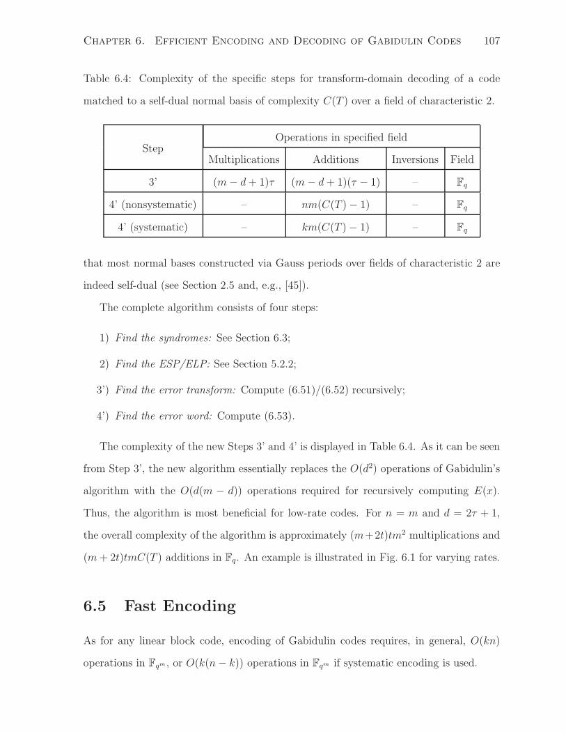
Chapter 6. Efficient Encoding and Decoding of Gabidulin Codes 107
Table 6.4: Complexity of the specific steps for transform-domain decoding of a code
matched to a self-dual normal basis of complexity C(T ) over a field of characteristic 2.
StepOperations in specified field
Multiplications Additions Inversions Field
3’ (m − d + 1)τ (m − d + 1)(τ − 1) – Fq
4’ (nonsystematic) – nm(C(T ) − 1) – Fq
4’ (systematic) – km(C(T ) − 1) – Fq
that most normal bases constructed via Gauss periods over fields of characteristic 2 are
indeed self-dual (see Section 2.5 and, e.g., [45]).
The complete algorithm consists of four steps:
1) Find the syndromes: See Section 6.3;
2) Find the ESP/ELP: See Section 5.2.2;
3’) Find the error transform: Compute (6.51)/(6.52) recursively;
4’) Find the error word: Compute (6.53).
The complexity of the new Steps 3’ and 4’ is displayed in Table 6.4. As it can be seen
from Step 3’, the new algorithm essentially replaces the O(d2) operations of Gabidulin’s
algorithm with the O(d(m − d)) operations required for recursively computing E(x).
Thus, the algorithm is most beneficial for low-rate codes. For n = m and d = 2τ + 1,
the overall complexity of the algorithm is approximately (m+2t)tm2 multiplications and
(m + 2t)tmC(T ) additions in Fq. An example is illustrated in Fig. 6.1 for varying rates.
6.5 Fast Encoding
As for any linear block code, encoding of Gabidulin codes requires, in general, O(kn)
operations in Fqm, or O(k(n − k)) operations in Fqm if systematic encoding is used.
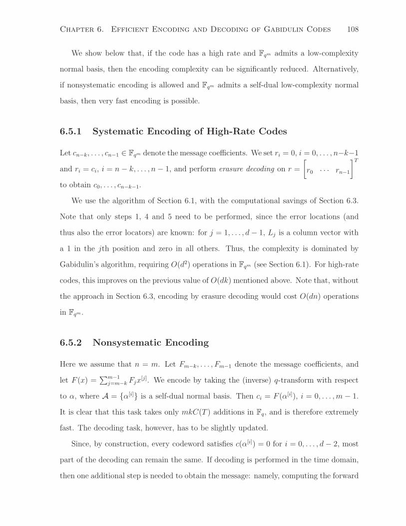
Chapter 6. Efficient Encoding and Decoding of Gabidulin Codes 108
We show below that, if the code has a high rate and Fqm admits a low-complexity
normal basis, then the encoding complexity can be significantly reduced. Alternatively,
if nonsystematic encoding is allowed and Fqm admits a self-dual low-complexity normal
basis, then very fast encoding is possible.
6.5.1 Systematic Encoding of High-Rate Codes
Let cn−k, . . . , cn−1 ∈ Fqm denote the message coefficients. We set ri = 0, i = 0, . . . , n−k−1
and ri = ci, i = n − k, . . . , n − 1, and perform erasure decoding on r =
[
r0 · · · rn−1
]T
to obtain c0, . . . , cn−k−1.
We use the algorithm of Section 6.1, with the computational savings of Section 6.3.
Note that only steps 1, 4 and 5 need to be performed, since the error locations (and
thus also the error locators) are known: for j = 1, . . . , d − 1, Lj is a column vector with
a 1 in the jth position and zero in all others. Thus, the complexity is dominated by
Gabidulin’s algorithm, requiring O(d2) operations in Fqm (see Section 6.1). For high-rate
codes, this improves on the previous value of O(dk) mentioned above. Note that, without
the approach in Section 6.3, encoding by erasure decoding would cost O(dn) operations
in Fqm.
6.5.2 Nonsystematic Encoding
Here we assume that n = m. Let Fm−k, . . . , Fm−1 denote the message coefficients, and
let F (x) =∑m−1
j=m−k Fjx[j]. We encode by taking the (inverse) q-transform with respect
to α, where A = α[i] is a self-dual normal basis. Then ci = F (α[i]), i = 0, . . . , m − 1.
It is clear that this task takes only mkC(T ) additions in Fq, and is therefore extremely
fast. The decoding task, however, has to be slightly updated.
Since, by construction, every codeword satisfies c(α[i]) = 0 for i = 0, . . . , d − 2, most
part of the decoding can remain the same. If decoding is performed in the time domain,
then one additional step is needed to obtain the message: namely, computing the forward

Chapter 6. Efficient Encoding and Decoding of Gabidulin Codes 109
q-transform Fj = c(α[j]), for j = m − k, . . . , m − 1. These extra mkC(T ) additions in
Fq barely affect the decoding complexity. On the other hand, if decoding is performed
in the transform domain, than the last step (obtaining e(x) from E(x)) can be simply
skipped, as F (x) = R(x) − E(x). This further saves at least mkC(T ) additions in Fq.
6.6 Practical Considerations
We have seen that the complexity of decoding a Gabidulin code C ⊆ Fn×mq with dR(C) = d
is given by O(dm) operations in Fqm. In many applications, in particular for network
coding, we have m ≫ n. In such cases, the decoding complexity can be significantly
reduced by using, rather than a Gabidulin code, an MRD code formed by the Cartesian
product of many shorter Gabidulin codes with the same distance. More precisely, let
ℓ = ⌊mn⌋ and n′ = m − n(ℓ − 1). Take C = C1 × C2 × · · · × Cℓ, where Ci ⊆ Fn×n
q ,
i = 1, . . . , ℓ − 1, and Cℓ ⊆ Fn×n′
q are Gabidulin codes with minimum rank distance d.
Then, according to Theorem 2.2, C is an MRD code with dR(C) = d.
Now, decoding of C can be performed by decoding each Ci individually. Thus, assum-
ing for simplicity that m = nℓ, the overall decoding complexity is given by ℓO(dn) =
O(dm) operations in Fqn. In other words, operations in a potentially large field Fqm can
be replaced by operations in a much smaller field Fqn.
Note that, in this case, additional computational savings may be obtained, since all
received words will share the same set of error locations. For instance, if all error locations
are known and the decoding algorithm of Section 6.1 is used, then only steps 1 and 4–6
need to be performed.

Chapter 7
Error Control under a Probabilistic
Error Model
In this chapter, we turn our attention to the LNCC under a probabilistic error model.
In particular, we investigate the noncoherent channel described by the channel law
Y = AX + DZ (7.1)
where A ∈ Tn×n, D ∈ Tn,t and Z ∈ Tt×m are chosen uniformly at random and indepen-
dently from other variables. Our main objective is to derive approximate expressions for
the capacity of this channel and to devise efficient capacity-achieving schemes.
We start by highlighting the main differences between our approaches for adversarial
and probabilistic channels. Then, we proceed by analyzing two simple channels: a mul-
tiplicative matrix channel, in Section 7.2, and an additive matrix channel, in Section 7.3.
The multiplicative channel can be seen as a special case of (7.1) when no errors occur.
The additive channel, on the other hand, can be seen as a coherent LNCC such that
the transfer matrix is invertible. For both channels, we compute the exact capacity and
propose simple capacity-achieving schemes. In Section 7.4, we combine both approaches
to produce an additive-multiplicative matrix channel that is equivalent to (7.1). For this
channel, we can only provide upper and lower bounds on the capacity, but we show that
110

Chapter 7. Error Control under a Probabilistic Error Model 111
these bounds match when either the field size or the packet length grows to infinity.
We also propose a simple capacity-achieving scheme based on the ideas of Sections 7.2
and 7.3. Finally, in Section 7.5, we discuss extensions to the results of this chapter, such
as the case where the error matrix may have variable rank.
The problem of error control in network coding under a probabilistic error model was
initially suggested in [23], which provided the motivation for this chapter. The authors
in [23] proposed a coding scheme based on random sparse graphs and iterative decoding.
However, besides not being capacity-achieving, the scheme of [23] has significantly high
decoding complexity (O(n3m)) and a relatively slow decay in the probability of error.
The scheme we propose not only is capacity-achieving but also has a lower decoding
complexity (O(n2m)) and a better decay in the probability of failure—besides being
conceptually much simpler.
7.1 Matrix Channels
For clarity and consistency of notation, we recall a few definitions from information
theory [64].
A discrete channel (X ,Y , pY |X) consists of an input alphabet X , an output alphabet
Y , and a conditional probability distribution pY |X relating the channel input X ∈ X and
the channel output Y ∈ Y . An (M, ℓ) code for a channel (X ,Y , pY |X) consists of an
encoding function 1, . . . , M → X ℓ and a decoding function Yℓ → 1, . . . , M, f, where
f denotes a decoding failure. It is understood that an (M, ℓ) code is applied to the ℓth
extension of the discrete memoryless channel (X ,Y , pY |X). A rate R (in bits) is said to be
achievable if there exists a sequence of (⌈2ℓR⌉, ℓ) codes such that decoding is unsuccessful
(either an error or a failure occurs) with probability arbitrarily small as ℓ → ∞. The
capacity of the channel is the supremum of all achievable rates. It is well-known that the

Chapter 7. Error Control under a Probabilistic Error Model 112
capacity is given by
C = maxpX
I(X; Y )
where pX denotes the input distribution.
Here, we are interested in matrix channels, i.e., channels for which both the input
and output variables are matrices. In particular, we are interested in a family of additive
matrix channels given by the channel law
Y = AX + DZ (7.3)
where X, Y ∈ Fn×mq , A ∈ Fn×n
q , D ∈ Fn×tq , Z ∈ Ft×m
q , and X, (A, D) and Z are statisti-
cally independent. Since the capacity of a matrix channel naturally scales with nm, we
also define a normalized capacity
C =1
nmC.
In the following, we assume that statistics of A, D and Z are given for all q, n, m, t.
In this case, we may denote a matrix channel simply by the tuple (q, n, m, t), and we
may also indicate this dependency in both C and C. We now define two limiting forms
of a matrix channel (strictly speaking, of a sequence of matrix channels). The first form,
which we call the infinite-field-size channel, is obtained by taking q → ∞. The capacity
of this channel is given by
limq→∞
1
log2 qC(q, n, m, t)
represented in q-ary units per channel use. The second form, which we call the infinite-
rank channel, is obtained by setting t = τn and n = λm, and taking m → ∞. The
normalized capacity of this channel is given by
limm→∞
1
log2 qC(q, λm, m, τλm)

Chapter 7. Error Control under a Probabilistic Error Model 113
represented in q-ary units per transmitted q-ary symbol. We will hereafter assume that
logarithms are taken to the base q and omit the factor 1log2 q
from the above expressions.
Note that, to achieve the capacity of an infinite-field-size channel (similarly for an
infinite-rank channel), one should find a two-dimensional family of codes: namely, a
sequence of codes with increasing block length ℓ for each q, as q → ∞ (or for each m, as
m → ∞).
We will simplify our task here by considering only codes with block length ℓ = 1,
which we call one-shot codes. We will show, however, that these codes can achieve the
capacity of both the infinite-field-size and the infinite-rank channels, at least for the
classes of channels considered here. In other words, one-shot codes are asymptotically
optimal as either q → ∞ or m → ∞.
For completeness, we define also two more versions of the channel: the infinite-packet-
length channel, obtained by fixing q, t and n, and letting m → ∞, and the infinite-batch-
size channel, obtained by fixing q, t and m, and letting n → ∞. These channels will only
be discussed in Section 7.5.5.
It is important to note that a (q, n, ℓm, t) channel is not the same as the ℓ-extension
of a (q, n, m, t) channel. For instance, the 2-extension of a (q, n, m, t) channel has channel
law
(Y1, Y2) = (A1X1 + D1Z1, A2X2 + D2Z2)
where (X1, X2) ∈(Fn×m
q
)2, and (A1, D1, Z1) and (A2, D2, Z2) correspond to independent
realizations of a (q, n, m, t) channel. This is not the same as the channel law for a
(q, n, 2m, t) channel,
[
Y1 Y2
]
= A1
[
X1 X2
]
+ D1
[
Z1 Z2
]
since (A2, D2) may not be equal to (A1, D1). This should be contrasted to the models used
in [16] and [23]. Although both models are referred to simply as “random linear network
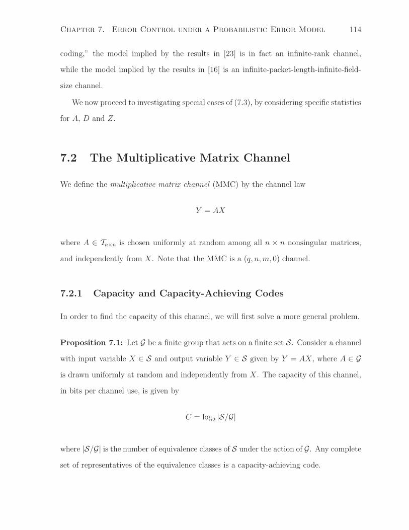
Chapter 7. Error Control under a Probabilistic Error Model 114
coding,” the model implied by the results in [23] is in fact an infinite-rank channel,
while the model implied by the results in [16] is an infinite-packet-length-infinite-field-
size channel.
We now proceed to investigating special cases of (7.3), by considering specific statistics
for A, D and Z.
7.2 The Multiplicative Matrix Channel
We define the multiplicative matrix channel (MMC) by the channel law
Y = AX
where A ∈ Tn×n is chosen uniformly at random among all n × n nonsingular matrices,
and independently from X. Note that the MMC is a (q, n, m, 0) channel.
7.2.1 Capacity and Capacity-Achieving Codes
In order to find the capacity of this channel, we will first solve a more general problem.
Proposition 7.1: Let G be a finite group that acts on a finite set S. Consider a channel
with input variable X ∈ S and output variable Y ∈ S given by Y = AX, where A ∈ G
is drawn uniformly at random and independently from X. The capacity of this channel,
in bits per channel use, is given by
C = log2 |S/G|
where |S/G| is the number of equivalence classes of S under the action of G. Any complete
set of representatives of the equivalence classes is a capacity-achieving code.

Chapter 7. Error Control under a Probabilistic Error Model 115
Proof: For each x ∈ S, let G(x) = gx | g ∈ G denote the orbit of x under the action
of G. Recall that G(y) = G(x) for all y ∈ G(x) and all x ∈ S, that is, the orbits form
equivalence classes.
For y ∈ G(x), let Gx,y = g ∈ G | gx = y. By a few manipulations, it is easy to show
that |Gx,y| = |Gx,y′| for all y, y′ ∈ G(x). Since A has a uniform distribution, it follows that
P [Y = y | X = x] = 1/|G(x)|, for all y ∈ G(x).
For any x ∈ S, consider the same channel but with the input alphabet restricted to
G(x). Note that the output alphabet will also be restricted to G(x). This is a |G(x)|-ary
channel with uniform transition probabilities; thus, the capacity of this channel is 0. Now,
the overall channel can be considered as a sum (union of alphabets) of all the restricted
channels. The capacity of a sum of M channels with capacities Ci, i = 1, . . . , M , is
known to be log2
∑Mi=1 2Ci bits. Thus, the capacity of the overall channel is log2 M bits,
where M = |S/G| is the number of orbits. A capacity-achieving code (with block length
1) may be obtained by simply selecting one representative from each equivalence class.
Proposition 7.1 shows that in a channel induced by a group action, where the group
elements are selected uniformly at random, the receiver cannot distinguish between trans-
mitted elements that belong to the same equivalence class. Thus, the transmitter can
only communicate the choice of a particular equivalence class.
Returning to our original problem, we have S = Fn×mq and G = Tn×n (the general
linear group GLn(Fq)). The equivalence classes of S under the action of G are the sets
of matrices that share the same row space. Thus, we can identify each equivalence class
with a subspace of Fmq of dimension at most n. Recall that the Gaussian coefficient
[m
k
]
q
=k−1∏
i=0
(qm − qi)/(qk − qi)
denotes the number of k-dimensional subspaces of Fmq . We have the following corollary
of Proposition 7.1.
Chapter 7. Error Control under a Probabilistic Error Model 116
Corollary 7.2: The capacity of the MMC, in q-ary units per channel use, is given by
CMMC = logq
n∑
k=0
[m
k
]
q
.
A capacity-achieving code C ⊆ Fn×mq can be obtained by ensuring that each k-dimensional
subspace of Fmq , k ≤ n, is the row space of some unique X ∈ C.
Note that Corollary 7.2 reinforces the idea introduced in [18] that, in order to com-
municate under random network coding, the transmitter should encode information in
the choice of a subspace (see Section 4.3).
We now compute the capacity for the two limiting forms of the channel, as discussed
in Section 7.1. We have the following result.
Proposition 7.3: Let λ = n/m and assume 0 < λ ≤ 1/2. Then
limq→∞
CMMC = (m − n)n (7.13)
limm→∞n=λm
CMMC = 1 − λ. (7.14)
Proof: First, observe that
[m
n∗
]
q
<
n∑
k=0
[m
k
]
q
< (n + 1)
[m
n∗
]
q
(7.15)
where n∗ = minn, ⌊m/2⌋. Using (2.12), it follows that
(m − n∗)n∗ < CMMC < (m − n∗)n∗ + logq 4(n + 1). (7.16)
The last term on the right vanishes on both limiting cases.
The case λ ≥ 1/2 can also be readily obtained but is less interesting since, in practice,
the packet length m will be much larger than the number of packets n.
Note that an expression similar to (7.16) has been found in [65] under a different
assumption on the transfer matrix (namely, that A is uniform on Fn×nq ). It is interesting
Chapter 7. Error Control under a Probabilistic Error Model 117
to note that, also in that case, the same conclusion can be reached about the sufficiency
of transmitting subspaces [65].
An intuitive way to interpret (7.13) is the following: out of the nm symbols obtained
by the receiver, n2 of these symbols are used to describe A, while the remaining ones are
used to communicate X.
Note that both limiting capacity expressions (7.13) and (7.14) can be achieved using
a simple coding scheme where an n× (m− n) data matrix U is concatenated on the left
with an n× n identity matrix I, yielding a transmitted matrix X =
[
I U
]
. The first n
symbols of each transmitted packet may be interpreted as pilot symbols used to perform
“channel sounding”. Observe that this is simply the standard way of using random
network coding (see Section 3.1; compare also with the lifting approach of Section 4.3.3).
7.3 The Additive Matrix Channel
We define the additive matrix channel (AMC) according to
Y = X + W
where W ∈ Tn×m,t is chosen uniformly at random among all n × m matrices of rank t,
independently from X. Note that the AMC is a (q, n, m, t) channel with D ∈ Tn×t and
Z ∈ Tt×m uniformly distributed, and A = I.
7.3.1 Capacity
The capacity of the AMC is computed in the next proposition.
Proposition 7.4: The capacity of the AMC is given by
CAMC = nm − logq |Tn×m,t|.

Chapter 7. Error Control under a Probabilistic Error Model 118
For λ = n/m and τ = t/n, we have the limiting expressions
limq→∞
CAMC = (m − t)(n − t) (7.19)
limm→∞n=λmt=τn
CAMC = (1 − λτ)(1 − τ). (7.20)
Proof: To compute the capacity, we expand the mutual information
I(X; Y ) = H(Y ) − H(Y |X) = H(Y ) − H(W )
where the last equality holds because X and W are independent. Note that H(Y ) ≤ nm,
and the maximum is achieved when Y is uniform. Since H(W ) does not depend on the
input distribution, we can maximize H(Y ) by choosing, e.g., a uniform pX .
The entropy of W is given by H(W ) = logq |Tn×m,t|. The number of n × m matrices
of rank t is given by (2.15)
|Tn×m,t| = q(n+m−t)t
t−1∏
i=0
(1 − qi−n)(1 − qi−m)
(1 − qi−t).
Thus,
CAMC = nm − logq |Tn×m,t|
= (m − t)(n − t) + logq
t−1∏
i=0
(1 − qi−t)
(1 − qi−n)(1 − qi−m)
The limiting expressions (7.19) and (7.20) follow immediately from the equation above.
As can be seen from (2.15), an n×m matrix of rank t can be specified with approxi-
mately (n+m− t)t symbols. Thus, the capacity (7.19) can be interpreted as the number
of symbols conveyed by Y minus the number of symbols needed to describe W .
7.3.2 A Coding Scheme
We now present an efficient coding scheme that achieves (7.19) and (7.20). The scheme
is based on an “error trapping” strategy.

Chapter 7. Error Control under a Probabilistic Error Model 119
Let U ∈ F(n−v)×(m−v)q be a data matrix, where v ≥ t. A codeword X is formed by
adding all-zero rows and columns to U so that
X =
0v×v 0v×(m−v)
0(n−v)×v U
.
These all-zero rows and columns may be interpreted as the “error traps.” Clearly, the
rate of this scheme is R = (n − v)(m − v).
Since the noise matrix W has rank t, we can write it as
W = BZ =
B1
B2
[
Z1 Z2
]
where B1 ∈ Fv×tq , B2 ∈ F
(n−v)×tq , Z1 ∈ Ft×v
q and Z2 ∈ Ft×(m−v)q . The received matrix Y is
then given by
Y = X + W =
B1Z1 B1Z2
B2Z1 U + B2Z2
.
We define an error trapping failure to be the event that rank B1Z1 < t. Intuitively,
this corresponds to the situation where either the row space or the column space of the
error matrix has not been “trapped”.
For now, assume that the error trapping is successful, i.e., rank B1 = rank Z1 = t.
Consider the submatrix corresponding to the first v columns of Y . Since rank B1Z1 = t,
the rows of B2Z1 are completely spanned by the rows of B1Z1. Thus, there exists some
matrix T such that B2Z1 = TB1Z1. But (B2 − TB1)Z1 = 0 implies that B2 − TB1 = 0,
since Z1 has full row rank. It follows that
T
B1
B2
=
B1
0
, where T =
I 0
T I
.

Chapter 7. Error Control under a Probabilistic Error Model 120
Note also that TX = X. Thus,
TY = TX + TW =
B1Z1 B1Z2
0 U
from which the data matrix U can be readily obtained.
The complexity of the scheme is computed as follows. In order to obtain T , it suffices
to perform Gaussian elimination on the left n × v submatrix of Y , for a cost of O(nv2)
operations. The data matrix can be extracted by multiplying T with the top right
v× (n−v) submatrix of Y , which can be accomplished in O((n−v)v(m−v)) operations.
Thus, the overall complexity of the scheme is O(nmv) operations in Fq.
Note that B1Z1 is available at the receiver as the top-left submatrix of Y . Moreover,
the rank of B1Z1 is already computed during the Gaussian elimination step of the decod-
ing. Thus, the event that the error trapping fails can be readily detected at the receiver,
which can then declare a decoding failure. It follows that the error probability of the
scheme is zero.
Let us now compute the probability of decoding failure. Consider, for instance, P1 =
P [rank Z1 = t], where Z =
[
Z1 Z2
]
is a full-rank matrix chosen uniformly at random.
An equivalent way of generating Z is to first generate the entries of a matrix M ∈ Ft×mq
uniformly at random, and then discard M if it is not full-rank. Thus, we want to compute
P1 = P [rank M1 = t | rank M = t], where M1 corresponds to the first v columns of M .
This probability is
P1 =P [rank M1 = t]
P [rank M = t]=
qmt∏t−1
i=0(qv − qi)
qvt∏t−1
i=0(qm − qi)
>
t−1∏
i=0
(1 − qi−v) ≥ (1 − qt−1−v)t ≥ 1 − t
q1+v−t.
The same analysis holds for P2 = P [rank B1 = t]. By the union bound, it follows that
the probability of failure satisfies
Pf <2t
q1+v−t. (7.28)

Chapter 7. Error Control under a Probabilistic Error Model 121
Proposition 7.5: The coding scheme described above can achieve both capacity expres-
sions (7.19) and (7.20).
Proof: From (7.28), we see that achieving either of the limiting capacities amounts to
setting a suitable v. To achieve (7.19), we set v = t and let q grow. The resulting code
will have the correct rate, namely, R = (n−t)(m−t) in q-ary units, while the probability
of failure will decrease exponentially with the field size in bits.
Alternatively, to achieve (7.20), we can choose some small ǫ > 0 and set v = (τ + ǫ)n,
where both τ = t/n and λ = n/m are assumed fixed. By letting m grow, we obtain
a probability of failure that decreases exponentially with m. The (normalized) gap to
capacity of the resulting code will be
g , limm→∞
CAMC − R/(nm)
= (1 − λτ)(1 − τ) − (1 − λ(τ + ǫ))(1 − (τ + ǫ))
= λǫ(1 − (τ + ǫ)) + ǫ(1 − λτ)
< λǫ + ǫ = (1 + λ)ǫ
which can be made as small as we wish.
7.4 The Additive-Multiplicative Matrix Channel
Let us now return to the LNCC described in (7.1). Since A is invertible, we can rewrite
(7.1) as
Y = AX + DZ = A(X + A−1DZ). (7.29)
Now, since Tn×n acts transitively on Tn×t, the channel law (7.29) is equivalent to
Y = A(X + W ) (7.30)
where A ∈ Tn×n and W ∈ Tn×m,t are chosen uniformly at random and independently from
any other variables. We call (7.30) the additive-multiplicative matrix channel (AMMC).

Chapter 7. Error Control under a Probabilistic Error Model 122
7.4.1 Capacity
One of the main results of this section is the following theorem, which provides an upper
bound on the capacity of the AMMC.
Theorem 7.6: For n ≤ m/2, the capacity of the AMMC is upper bounded by
CAMMC ≤ (m − n)(n − t) + logq 4(1 + n)(1 + t).
Proof: Let S = X + W . By expanding I(X, S; Y ), and using the fact that X, S and Y
form a Markov chain, in that order, we have
I(X; Y ) = I(S; Y ) − I(S; Y |X) + I(X; Y |S)︸ ︷︷ ︸
=0
= I(S; Y ) − I(W ; Y |X)
= I(S; Y ) − H(W |X) + H(W |X, Y )
= I(S; Y ) − H(W ) + H(W |X, Y ) (7.32)
≤ CMMC − logq |Tn×m,t| + H(W |X, Y ) (7.33)
where (7.32) follows since X and W are independent.
We now compute an upper bound on H(W |X, Y ). Let R = rank Y and write Y = GY ,
where G ∈ Tn×R and Y ∈ TR×m. Note that
X + W = A−1Y = A−1GY = A∗Y
where A∗ = A−1G. Since Y is full-rank, it must contain an invertible R×R submatrix. By
reordering columns if necessary, assume that the left R×R submatrix of Y is invertible.
Write Y =
[
Y1 Y2
]
, X =
[
X1 X2
]
and W =
[
W1 W2
]
, where Y1, X1 and W1 have
R columns, and Y2, X2 and W2 have m − R columns. We have
A∗ = (X1 + W1)Y−11 and W2 = A∗Y2 − X2.

Chapter 7. Error Control under a Probabilistic Error Model 123
It follows that W2 can be computed if W1 is known. Thus,
H(W |X, Y ) = H(W1|X, Y ) ≤ H(W1|R) ≤ H(W1|R = n)
≤ logq
t∑
i=0
|Tn×n,i| ≤ logq(t + 1)|Tn×n,t| (7.36)
where (7.36) follows since W1 may possibly be any n × n matrix with rank ≤ t.
Applying this result in (7.33), and using (7.15) and (2.14), we have
I(X, Y ) ≤ logq(n + 1)
[m
n
]
+ logq(t + 1)|Tn×t|
[nt
]
|Tn×t|[mt
]
≤ logq(n + 1)(t + 1)
[m − t
n − t
]
(7.37)
≤ (m − n)(n − t) + logq 4(1 + n)(1 + t).
where (7.37) follows from 2.13.
We now develop a connection with the subspace approach of [18] (see also Section 4.3)
that will be useful to obtain a lower bound on the capacity. From Section 7.2, we
know that, in a multiplicative matrix channel, the receiver can only distinguish between
transmitted subspaces. Thus, we can equivalently express
CAMMC = maxpX
I(X ;Y)
where X and Y denote the row spaces of X and Y , respectively.
Using this interpretation, we can obtain the following lower bound on capacity.
Theorem 7.7: Assume n ≤ m. For any ǫ ≥ 0, we have
CAMMC ≥ (m − n)(n − t − ǫt) − logq 4 − 2tnm
q1+ǫt.
In order to prove Theorem 7.7, we need a few lemmas.
Chapter 7. Error Control under a Probabilistic Error Model 124
Lemma 7.8: Let X ∈ Fn×mq be a matrix of rank k, and let W ∈ Fn×m
q be a random
matrix chosen uniformly among all matrices of rank t. If k + t ≤ minn, m, then
P [rank(X + W ) < k + t] <2t
qminn,m−k−t+1.
Proof: Write X = X ′X ′′, where X ′ ∈ Fn×kq and X ′′ ∈ Fk×m
q are full-rank matrices. We
can generate W as W = W ′W ′′, where W ′ ∈ Tn×t and W ′′ ∈ Tt×m are chosen uniformly
at random and independently from each other. Then we have
X + W = X ′X ′′ + W ′W ′′ =
[
X ′ W ′
]
X ′′
W ′′
.
Note that rank(X + W ) = k + t if and only if the column spaces of X ′ and W ′ intersect
trivially and the row spaces of X ′′ and W ′′ intersect trivially. Let P ′ and P ′′ denote the
probabilities of these two events, respectively. By a simple counting argument, we have
P ′ =(qn − qk) · · · (qn − qk+t−1)
(qn − 1) · · · (qn − qt−1)=
t−1∏
i=0
(1 − qk−n+i)
(1 − q−n+i)
>
t−1∏
i=0
(1 − qk−n+i) ≥ (1 − qk−n+t−1)t ≥ 1 − tqk−n+t−1.
Similarly, we have P ′′ > 1 − tqk−m+t−1. Thus,
P [rank(X + W ) < k + t] <t
qn−k−t+1+
t
qm−k−t+1
≤ 2t
qminn,m−k−t+1.
For dim X ≤ n ≤ m, let SX ,n denote the set of all n-dimensional subspaces of Fmq
that contain a subspace X ⊆ Fmq .
Lemma 7.9:
|SX ,n| =
[m − k
n − k
]
q
where k = dim X .

Chapter 7. Error Control under a Probabilistic Error Model 125
Proof: By the fourth isomorphism theorem [66], there is a bijection between SX ,n and the
set of all (n− k)-dimensional subspaces of the quotient space Fmq /X . Since dim Fm
q /X =
m − k, the result follows.
We can now give a proof of Theorem 7.7.
Proof (of Theorem 7.7): Assume that X is selected from Tn×m,k, where k = n−(1+ǫ)t
and ǫ ≥ 0. Define a random variable Q as
Q =
1 if dim Y = rank(X + W ) = k + t
0 otherwise.
Note that X ⊆ Y when Q = 1.
By Lemma 7.9 and (2.12), we have
H(Y|X , Q = 1) ≤ logq |SX ,n′| ≤ (m − n′)t + logq 4
where n′ = k+t. Choosing X uniformly from Tn×m,k, we can also make Y uniform within
a given dimension; in particular,
H(Y|Q = 1) = logq
[m
n′
]
q
≥ (m − n′)n′.
It follows that
I(X ;Y|Q = 1) = H(Y|Q = 1) − H(Y|X , Q = 1)
≥ (m − n′)(n′ − t) − logq 4
≥ (m − n)(n − t − ǫt) − logq 4.

Chapter 7. Error Control under a Probabilistic Error Model 126
Now, using Lemma 7.8, we obtain
I(X ;Y) = I(X ;Y , Q) = I(X ; Q) + I(X ;Y|Q)
≥ I(X ;Y|Q)
≥ P [Q = 1]I(X ;Y|Q = 1)
≥ I(X ;Y|Q = 1) − P [Q = 0]nm
≥ (m − n)(n − t − ǫt) − logq 4 − 2tnm
qǫt+1.
Note that, differently from the results of previous sections, Theorems 7.6 and 7.7
provide only upper and lower bounds on the channel capacity. Nevertheless, it is still
possible to compute exact expressions for the capacity of the AMMC in certain limiting
cases.
Corollary 7.10: For 0 < λ = n/m ≤ 1/2 and τ = t/n, we have
limq→∞
CAMMC = (m − n)(n − t) (7.46)
limm→∞n=λmt=τn
CAMMC = (1 − λ)(1 − τ). (7.47)
Proof: The fact that the values in (7.46) and (7.47) are upper bounds follows immedi-
ately from Theorem 7.6. The fact that (7.46) is a lower bound follows immediately from
Theorem 7.7 by setting ǫ = 0. To obtain (7.47) from Theorem 7.7, it suffices to choose ǫ
such that 1/ǫ grows sublinearly with m, e.g., ǫ = 1/√
m.
Differently from the MMC and the AMC, successful decoding in the AMMC does
not (necessarily) allow recovery of all sources of channel uncertainty—in this case, the
matrices A and W . In general, for every observable (X, Y ) pair, there are many valid
A and W such that Y = A(X + W ). Such coupling between A and W is reflected in
extra term H(W |X, Y ) in (7.32), which provides an additional rate of roughly (2n − t)t
as compared to the straightforward lower bound CAMMC ≥ CMMC − logq |Tn×m,t| ≈ (m−
n)n − (n + m − t)t.

Chapter 7. Error Control under a Probabilistic Error Model 127
Remark: In [23], the problem of finding the capacity of the AMMC was addressed using
a specific form of transmission matrices that contained an n × n identity header. This
approach, in fact, turns the channel into an AMC after stripping off the headers. It is
instructive to observe that the capacity expression of [23], C = (1 − λ − λτ)(1 − τ),
corresponds exactly to (7.20) after accounting for the extra redundancy in the header
(i.e., replacing m with m − n). We might, therefore, interpret that [23] has computed
the capacity of the infinite-rank AMC. The statement of Proposition 7.4 is, nevertheless,
(slightly) more general than that of [23]. Note that, as the input distribution assumed
in [23] is not capacity-achieving, the capacity of the infinite-rank AMMC (7.47) is strictly
larger than the expression obtained in [23].
7.4.2 A Coding Scheme
We now propose an efficient coding scheme that can asymptotically achieve (7.46) and
(7.47). The scheme is based on a combination of channel sounding and error trapping
strategies.
For a data matrix U ∈ F(n−v)×(m−n)q , where v ≥ t, let the corresponding codeword be
X =
0
X
=
0v×v 0v×(n−v) 0v×(m−n)
0(n−v)×v I(n−v)×(n−v) U
.
Note that the all-zero matrices provide the error traps, while the identity matrix corre-
sponds to the pilot symbols. Clearly, the rate of this scheme is R = (n − v)(m − n).
Write the noise matrix W as
W = BZ =
B1
B2
[
Z1 Z2 Z3
]
where B1 ∈ Fv×tq , B2 ∈ F
(n−v)×tq , Z1 ∈ Ft×v
q , Z2 ∈ Ft×(n−v)q and Z3 ∈ F
t×(m−n)q . The

Chapter 7. Error Control under a Probabilistic Error Model 128
auxiliary matrix S is then given by
S = X + W =
B1Z1 B1Z2 B1Z3
B2Z1 I + B2Z2 U + B2Z3
.
Similarly as in Section 7.3, we define that the error trapping is successful if rank B1Z1 =
t. Assume that this is the case. From Section 7.3, there exists some matrix T ∈ Tn×n
such that
TS =
B1Z1 B1Z2 B1Z3
0 I U
=
B1 0
0 I
Z1 Z2 Z3
0 I U
.
Note further that
RRE
Z1 Z2 Z3
0 I U
=
Z1 0 Z3
0 I U
for some Z1 ∈ Ft×vq in RRE form and some Z3 ∈ F
t×(m−n)q . It follows that
RRE (S) = RRE
B1 0
0 I
Z1 Z2 Z3
0 I U
=
Z1 0 Z3
0 I U
0 0 0
where the bottom v − t rows are all-zeros.
Since A is invertible, we have RRE (Y ) = RRE (S), from which U can be readily
obtained. Thus, decoding amounts to performing Gauss-Jordan elimination on Y . It
follows that the complexity of the scheme is O(n2m) operations in Fq.
The probability that the error trapping is not successful, i.e., rank B1Z1 < t, was
computed in Section 7.3. Let A correspond to the first n columns of Y . Note that
rank B1Z1 = t if and only if rank A = n − v + t. Thus, when the error trapping is not
successful, the receiver can easily detect this event by looking at RRE (Y ) and then declare

Chapter 7. Error Control under a Probabilistic Error Model 129
a decoding failure. It follows that the scheme has zero error probability and probability
of failure given by (7.28).
Theorem 7.11: The proposed coding scheme can asymptotically achieve (7.46) and
(7.47).
Proof: Using (7.28) and the same argument as in the proof of Proposition 7.5, we can
set a suitable v in order to achieve arbitrarily low gap to capacity while maintaining an
arbitrary low probability of failure, for both cases where q → ∞ or m → ∞.
7.5 Extensions
In this section, we discuss possible extensions of the results and models presented in the
previous sections.
7.5.1 Dependent Transfer Matrices
As discussed in Section 7.4, the AMMC is equivalent to a channel of the form (7.3) where
A ∈ Tn×n and D ∈ Tn×t are chosen uniformly at random and independently from each
other. Suppose now that the channel is the same, except for the fact that A and D are not
independent. It should be clear that the capacity of the channel cannot be smaller than
that of the AMMC. For instance, one can always convert this channel into an AMMC
by employing randomization at the source. (This is, in fact, a natural procedure in any
random network coding system.) Let X = TX ′, where T ∈ Tn×n is chosen uniformly at
random and independent from any other variables. Then A′ = AT is uniform on Tn×n
and independent from D. Thus, the channel given by Y = A′X ′ + DZ is an AMMC.
Note that our coding scheme does not rely on any particular statistics of A given X
and W (except the assumption that A is invertible) and therefore works unchanged in
this case.

Chapter 7. Error Control under a Probabilistic Error Model 130
7.5.2 Transfer Matrix Invertible but Nonuniform
The model for the AMMC assumes that the transfer matrix A ∈ Tn×n is chosen uniformly
at random. In a realistic network coding system, the transfer matrix may be a function of
both the network code and the network topology, and therefore may not have a uniform
distribution. Consider the case where A is chosen according to an arbitrary probability
distribution on Tn×n. It should be clear that the capacity can only increase as compared
with the AMMC, since less “randomness” is introduced in the channel. The best possible
situation is to have a constant A, in which case the channel becomes exactly an AMC.
Again, note that our coding scheme for the AMMC is still applicable in this case.
7.5.3 Nonuniform Packet Errors
When expressed in the form (7.3), the models for both the AMC and the AMMC assume
that the matrix Z is uniformly distributed on Tn×t. In particular, each error packet is
uniformly distributed on F1×mq \ 0. In a realistic situation, however, it may be the case
that error packets of low weight are more likely to occur. Consider a model identical
to the AMC or the AMMC except for the fact that the matrix Z is chosen according
to an arbitrary probability distribution on Tt×m. Once again, it should be clear that
the capacity can only increase. Note that the exact capacity in Proposition 7.4 and the
upper bound of Theorem 7.6 can be easily modified to account for this case (by replacing
logq |Tn×m,t| with the entropy of W ).
Although our coding scheme in principle does not hold in this more general case, we
can easily convert the channel into an AMC or AMMC by applying a random transfor-
mation at the source (and its inverse at the destination). Let X = X ′T , where T ∈ Tm×m
is chosen uniformly at random and independent from any other variables. Then
Y ′ = Y T−1 = (AX + DZ)T−1 = AX ′ + DZ ′

Chapter 7. Error Control under a Probabilistic Error Model 131
where Z ′ = ZT−1. Since Tm×m acts (by right multiplication) transitively on Tt×m, we
have that Z ′ is uniform on Tt×m. Thus, we obtain precisely an AMMC (or AMC) and
the assumptions of our coding scheme hold.
Note, however, that, depending on the error model, the capacity may be much larger
than what can be achieved by the scheme described above. For instance, if the rows of Z
are constrained to have weight at most s (otherwise chosen, say, uniformly at random),
then the capacity would increase by approximately(m − s − logq
(ms
))t, which might be
a substantial amount if s is small.
7.5.4 Error Matrix with Variable Rank (≤ t)
The model we considered for the AMC and the AMMC assumes an error matrix W whose
rank is known and equal to t. It is useful to consider the case where rank W is allowed
to vary, while still bounded by t. More precisely, we assume that W is chosen uniformly
at random from Tn×m,R, where R ∈ 0, . . . , t is a random variable with probability
distribution P [R = r] = pr.
Since
H(W ) = H(W, R) = H(R) + H(W |R)
= H(R) +∑
r
prH(W |R = r)
= H(R) +∑
r
pr logq |Tn×m,r|
≤ H(R) + logq |Tn×m,t|,
we conclude that the capacities of the AMC and the AMMC may be reduced by at most
H(R) ≤ logq(t + 1). This loss is asymptotically negligible for large q and/or large m, so
the expressions (7.19), (7.20), (7.46) and (7.47) remain unchanged.
The steps for decoding and computing the probability of error trapping failure also
remain the same, provided we replace t by R. The only difference is that now decoding

Chapter 7. Error Control under a Probabilistic Error Model 132
errors may occur. More precisely, suppose that rank B1Z1 = t′ < t. A necessary condition
for success is that rank B1Z = rank BZ1 = t′. If this condition is not satisfied, then a
decoding failure is declared. However, if the condition is true, then the decoder cannot
determine whether t′ = R < t (an error trapping success) or t′ < R ≤ t (an error trapping
failure), and must proceed assuming the former case. If the latter case turns out to be
true, we would have an undetected error. Thus, for this model, the expression (7.28)
gives a bound on the probability that decoding is not successful, i.e., that either an error
or a failure occurs.
7.5.5 Infinite Packet Length or Infinite Batch Size
We now extend our results to the infinite-packet-length AMC and AMMC and the
infinite-batch-size AMC. (Note that, as pointed out in Section 7.2, there is little jus-
tification to consider an infinite-batch-size AMMC.) From the proof of Propositon 7.4
and the proof of Corollary 7.10, it is straightforward to see that
limm→∞
CAMMC = limm→∞
CAMC = (n − t)/n
limn→∞
CAMC = (m − t)/m.
It is not straightforward, however, to obtain capacity-achieving schemes for these
channels. The schemes described in Sections 7.3 and 7.4 for the infinite-rank AMC and
AMMC, respectively, use an error trap whose size (in terms of columns and rows) grows
proportionally with m (or n). While this is necessary for achieving vanishingly small error
probability, it also implies that these schemes are not suitable to the infinite-packet-length
channel (where m → ∞ but not n) or the infinite-batch-size channel (where n → ∞ but
not m).
In these situations, the proposed schemes can be adapted by replacing the data matrix
and part of the error trap with an MRD code. Consider first an infinite-packet-length

Chapter 7. Error Control under a Probabilistic Error Model 133
AMC. Let the transmitted matrix be given by
X =
[
0n×v x
]
(7.54)
where x ∈ Fn×(m−v)q is a codeword of a matrix code C. If (column) error trapping is
successful then, under the terminology of Section 5.2.2, the decoding problem for C
amounts to the correction of t erasures. As we know from Section 5.2.3, for m − v ≥ n,
an MRD code C ⊆ Fn×(m−v)q with rate (n− t)/n can correct exactly t erasures (with zero
probability of error) [27]. Thus, decoding fails if and only if column trapping fails.
Similarly, for an infinite-batch-size AMC, let the transmitted matrix be given by
X =
0v×m
x
where x ∈ F(n−v)×mq is a codeword of a matrix code C. If (row) error trapping is successful
then, under the terminology of Section 5.2.2, the decoding problem for C amounts to the
correction of t deviations. As we know from Section 5.2.3, for n − v ≥ m, an MRD code
C ⊆ F(n−v)×mq with rate (m− t)/m can correct exactly t deviations (with zero probability
of error). Thus, decoding fails if and only if row trapping fails.
Finally, for the infinite-packet-length AMMC, it is sufficient to prepend to (7.54) an
identity matrix, i.e.,
X =
[
In×n 0n×v x
]
.
The same reasoning as for the infinite-packet-length AMC applies here, and the decoder
in Chapter 5 is also applicable in this case.
For more details on the decoding of an MRD code combined with an error trap, we
refer the reader to [67]. The decoding complexity is in O(tn2m) and O(tm2n) (whichever
is smaller), and could be further simplified using the approach of Chapter 6.
In all cases, the schemes have probability of error upper bounded by t/q1+v−t and
therefore are capacity-achieving.

Chapter 8
Secure Network Coding
In this chapter, we divert our attention from the error control problem and instead focus
on the security issues that may arise when using network coding. We are interested
in addressing the problem of securing a linear network coding communication system
against a wiretapper adversary.
The scenario considered here has its roots in the wiretap channel II of Ozarow and
Wyner [19]. In this channel, a source transmits n symbols to a destination, µ of which
are observed by a wiretapper. The problem is how to encode a message into the n
transmitted symbols in such a way that the wiretapper gets no information about the
message (information-theoretic security). An optimal solution, proposed by Ozarow and
Wyner, is to use a coset coding scheme. The idea is to use the message to select a coset
of an MDS code, and transmit a random word within that coset. The randomization
does not affect the destination, but ensures that a wiretapper who observes only µ < n
symbols will not be able to uniquely identify the coset.
The wiretap channel II can be generalized to a network coding scenario [2–4] by
regarding the symbols as packets flowing through a network that implements linear net-
work coding. In this case, the wiretapper observes µ linear combinations of the original
packets. This problem, which became known as secure network coding, was first studied
134
Chapter 8. Secure Network Coding 135
by Cai and Yeung [20], and further investigated by Feldman et al. [21]. The connection
with the wiretap channel II was observed by Rouayheb and Soljanin [22].
In all of these works, the proposed solutions are essentially analogous to Ozarow-
Wyner’s coset coding scheme. However, the analogy breaks down in the fact that the
network may “undo” some of the randomization performed by the source, and actually
help the wiretapper. Thus, the network code and the outer code must be jointly designed
to prevent this “de-randomization.” A side-effect of this approach is that the field size
for network coding is required to be significantly large.
In Section 8.2, we propose a universal approach to network coding security that allows
a completely independent design. The idea (essentially a vector-linear approach) is to use
coset coding over an extension field of the field used for linear network coding operations.
This allows a complete separation between a “black-box” implementing network coding
and an outer security scheme. In particular, the network code need not be known, so a
our scheme is compatible with random network coding. A consequence of this approach
is that the field size for network coding can return to its usual values, i.e., as if security
were not a concern. Our scheme makes crucial use of the properties of MRD codes and
is shown to be optimal in a certain sense.
A drawback of enforcing security on a wiretap network is that the communication rate
must be reduced from n to n−µ, i.e., one “randomization” packet has to be spent for each
packet observed by the wiretapper. Hoping to overcome this rate barrier, Bhattad and
Narayanan [24] have defined a weaker notion of security that is practically very appealing.
Roughly speaking, a system is considered weakly secure if the wiretapper gets no infor-
mation about each packet individually, while still potentially obtaining “meaningless”
information about mixtures of packets. Under these more relaxed security requirements,
the maximum rate of n packets per message can be obtained. The approach of [24],
however, suffers from the same drawback as [20–22] in that the outer code has to be
carefully designed, and the field size required for network coding may be significantly

Chapter 8. Secure Network Coding 136
large. In Section 8.3, we show that a universal (i.e., network-code-independent) weakly
secure scheme can be obtained via an approach similar to that of Section 8.2.
A third contribution of this chapter, described in Section 8.4, is the design of a
universal scheme that can provide not only security but also protection against errors.
More precisely, we assume that the wiretapper is able not only to eavesdrop, but also to
inject up to t erroneous packets anywhere in the network. In this case, we can guarantee
security and reliability as long as µ + 2t < n. Other works have attained the same goals
under even looser conditions [16, 68], but these schemes were not universal. Once again,
advantages of our approach include the smaller field size and the simplicity of the design.
Finally, Section 8.5 discusses implementation aspects of our proposed schemes, which
are shown to be computationally efficient for both encoding and decoding.
8.1 The Wiretap Channel II
Let F be an arbitrary alphabet. Consider a communication system consisting of a source,
a destination and a wiretapper. The source produces a message S = (S1, S2, . . . , Sk), with
symbols S1, . . . , Sk drawn from F , and encodes this message as a word X = (X1, . . . , Xn),
Xi ∈ F . This word is transmitted over a noiseless channel and received by the destination.
The wiretapper has access to µ symbols of X, represented as the word W = (Xi, i ∈ I),
where I ⊆ 1, . . . , n has cardinality µ. The goal of the system is for the source to
communicate the message to the destination in such a way that the wiretapper cannot
obtain any information about S from any possible set of µ intercepted symbols. More
precisely, the conditions for secure communication are
H(S|X) = 0 (8.1)
I(S; W ) = 0, ∀I : |I| = µ. (8.2)
The objective is to design a (necessarily probabilistic) encoding of S into X such that
conditions (8.1) and (8.2) are satisfied.
Chapter 8. Secure Network Coding 137
It can be shown that the maximum number of symbols that can be securely commu-
nicated is upper bounded by H(S) ≤ n−µ (where the log is taken to the base |F |). This
maximum rate can be achieved, if F is a finite field of sufficiently large cardinality, by
using Ozarow-Wyner coset coding scheme [19]. The scheme can be described as follows.
Let k = n−µ and let C be a linear (n, µ) MDS code over F with parity-check matrix
H ∈ F k×n. Encoding is performed by choosing uniformly at random some X ∈ F n such
that S = HX, where S and X are taken as column vectors. In other words, each message
is viewed as a syndrome specifying a coset of C, and the transmitted vector is randomly
chosen among the elements of that coset. Upon reception of X, decoding is performed
by simply computing the syndrome S = HX.
It is useful to review the proof that this scheme is secure. By expanding I(S, X; W ),
we have
I(S; W ) = I(X; W ) + I(S; W |X)− I(X; W |S)
= H(W ) − H(W |X, S)− H(X|S) + H(X|S, W )
= H(W ) − H(X|S) + H(X|S, W ) (8.3)
= H(W ) − µ + H(X|S, W ) (8.4)
≤ H(X|S, W ) (8.5)
where (8.3) follows since W is a function of X, (8.4) follows since X is chosen uniformly
at random among |F |µ possibilities, and (8.5) follows since H(W ) ≤ µ. The last step is
to show that H(X|S, W ) = 0, i.e., that a word X can be determined given its coset, S,
and µ “non-erased” symbols, W . But this follows from the fact that C, as well as all of
its cosets, is an (n, µ) MDS code.

Chapter 8. Secure Network Coding 138
W
X YS
W = BX
source destination
adversary
Y = AX
Figure 8.1: Linear network coding channel with a wiretapper adversary.
8.2 Security for Wiretap Networks
For the remainder of this chapter we will use the following notation and terminology.
Packets transmitted over a network implementing linear network coding are drawn from
a set F , which is assumed to be an m-dimensional vector space over a finite field Fq.
A network using a network code that is feasible for the transmission of n packets from
source to (each) destination is called an (n, m, Fq)-linear multicast network.
8.2.1 Wiretap Networks
The wiretap problem of Section 8.1 can be generalized to a linear network coding scenario
by introducing a wiretapper in the setup of Section 3.1. The wiretapper can eavesdrop
on µ links, collectively represented by the set I; in this case, we will say that the network
is subject to µ observations. Since linear network coding is used, the packets observed by
the wiretapper are given by W = BX ∈ F µ, where B ∈ Fµ×nq is the matrix whose rows
are the global coding vectors associated with the edges in I. Additionally, we assume
that the “true” source message is given by S =
[
S1 S2 · · · Sk
]T
, Si ∈ F , which is then
encoded into X for transmission over the network. The system is depicted in Fig. 8.1.
Similarly as before, the conditions for secure communication are given by
H(S|Y ) = 0 (8.6)
I(S; W ) = 0, ∀I : |I| = µ. (8.7)

Chapter 8. Secure Network Coding 139
The problem, now, is how to design an encoding from S to X and a linear network code
such that (8.6) and (8.7) are satisfied.
Note that, since making a row of B linear dependent of the others cannot possibly
increase I(S; W ), we have that a necessary and sufficient (and therefore equivalent)
condition for (8.7) is given by
I(S; W ) = 0, ∀I : |I| = µ, rank B = µ. (8.8)
It is reasonable to assume that the network code used is feasible, i.e., that X can be
recovered from Y . If this is the case, then H(X|Y ) = 0 and thus condition (8.6) can
be replaced by (8.1). The problem then becomes very similar to that of Section 8.1, the
only difference being that the matrix B consists of row vectors over Fq rather then rows
from an identity matrix.
8.2.2 Security via Linear MDS Codes
The similarity mentioned above suggests that the same techniques that are useful for the
wiretap channel could also be useful for a wiretap network; namely, the Ozarow-Wyner
coset coding scheme discussed in Section 8.1. Note, however, that for that scheme to
be applicable, F must be a field. The case F = Fq was studied by Rouayheb and
Soljanin [22], who showed that secure communication at the maximum rate k = n − µ
can be achieved with a coset coding scheme if the network code is chosen to satisfy certain
constraints.
Let H be the parity-check matrix of a linear (n, µ) MDS code over F , and suppose
that a coset coding scheme based on H is used. Note that (8.1) follows immediately
from the fact that S = HX. In order to satisfy (8.8), we will make use of the following
proposition. We state the result in somewhat general terms since it will be useful later
on.

Chapter 8. Secure Network Coding 140
Proposition 8.1: Let F be a field, H ∈ F k×n and B ∈ F µ×n. Let S = Hx : x ∈ F n
and Xs = x ∈ F n : s = Hx. Let S ∈ S, X ∈ F n and W = BX be random variables.
1) If X is uniform over XS given S, then
rank
H
B
= rank H + rank B =⇒ I(S; W ) = 0.
2) If S is uniform, then
I(S; W ) = 0 =⇒ rank
H
B
= rank H + rank B.
Proof: See the Appendix.
A lightly weaker version of item 1) of Proposition 8.1 was proved in [22]. As we can
see from Proposition 8.1, condition (8.8) will be satisfied if the following condition holds:
rank
H
B
= n, ∀I : |I| = µ, rank B = µ. (8.11)
Equivalently, we must ensure that no linear combination of at most µ global coding
vectors belongs to the row space of H .
It follows from this result of Rouayheb and Soljanin that secure multicast communi-
cation can be achieved in two steps: first, designing a coset coding scheme based on an
MDS code, and then designing a linear network code so as to satisfy the above constraint.
Note that there is still a potentially undesirable coupling between the design of the
coset coding scheme and the design of the network code, as the latter must take H into
account. Moreover, the scheme is not compatible with random network coding, since
the network code must be carefully chosen so as to satisfy a large number of global
constraints.

Chapter 8. Secure Network Coding 141
8.2.3 Universal Security via MRD Codes
Dealing with the coupling mentioned above motivates the following definition of a uni-
versal scheme.
Definition 8.1: A secure communication scheme for a linear multicast network is called
universal if it provides security and reliability for any choice of a feasible linear network
code. That is, the scheme must satisfy conditions
H(S|X) = 0 (8.12)
I(S; W ) = 0, ∀B. (8.13)
By definition, a universal scheme is an outer code that can be designed independently
and applied on top of any (feasible) network code. The specific wiretapping matrix
B is irrelevant as long as at most µ observations are made by the wiretapper. As a
consequence, any such scheme is naturally compatible with random network coding.
We now present our construction of a universal secure communication scheme. Our
crucial assumption is that m, the dimension of F as a vector space over Fq, is at least n;
in other words, each packet must consist of m ≥ n symbols from Fq.
Our scheme is based on two main ideas: first, we regard F as an extension field of
Fq of degree m, denoted Fqm ; second, we replace the MDS code in Ozarow-Wyner coset
coding scheme by an MRD code over Fqm . Note that, since coset encoding/decoding
is performed only at source/destination nodes, setting F to be an extension field of Fq
does not interfere with the underlying linear network coding operations, which are still
performed over the base field Fq.
Let k = n−µ and let H be the parity-check matrix of a linear (n, µ) MRD code over
F = Fqm . Encoding and decoding of the source message S is performed as described in

Chapter 8. Secure Network Coding 142
Section 8.1. With respect to security, we must ensure that
rank
H
B
= n, ∀B : rank B = µ.
Note that, differently from Section 8.2.2, the matrix H is now defined over Fqm , while
the matrix B still has all its entries in Fq. This is the fundamental distinction of our
approach, which allows a complete decoupling of the outer code and the network code.
Our main result in this section is a consequence of the following theorem.
Theorem 8.2: Let C be a linear (n, µ) code over Fqm with parity-check matrix H ∈
F(n−µ)×nqm . Then C is an MRD code with m ≥ n if and only if the matrix
H
B
(8.15)
is nonsingular for any full-rank B ∈ Fµ×nq .
Proof: Let M denote the matrix in (8.15). We will show that dR(C) ≤ n−µ if and only
if there exists some full-rank B such that M is singular.
First, assume that dR(C) ≤ n − µ. Then there exists some nonzero x ∈ C such that
rank(x) ≤ n − µ. This implies that there exists some full-rank B ∈ Fµ×nq such that
Bx = 0. Thus, Mx = 0 and M is singular.
Conversely, assume that M is singular for some full-rank B ∈ Fµ×nq . Then there must
be some nonzero x ∈ F n such that Mx = 0. But this implies that Hx = 0, i.e., x ∈ C,
and Bx = 0, i.e., rank(x) ≤ n − µ. Thus, dR(C) ≤ n − µ.
We can now state the main result of this section.
Theorem 8.3: Consider an (n, m, Fq) linear multicast network subject to µ observa-
tions. Let H ∈ F(n−µ)×nqm be the parity-check matrix of a linear (n, µ) code over Fqm .
Universal secure communication at the maximum rate k = n− µ can be achieved with a

Chapter 8. Secure Network Coding 143
coset coding scheme based on H if and only if the code defined by H is an MRD code
with m ≥ n.
Proof: The achievability has been proved. The necessity part follows by combining item
2) of Proposition 8.1 with Theorem 8.2.
We now proceed to proving that our scheme is optimal, i.e., that there is no universal
scheme with m < n. First we need a couple of technical lemmas.
Lemma 8.4: Let S ∈ S, W ∈ W and X ∈ X be discrete random variables with
S = f(X) and W = g(X). Suppose S is uniform and |x ∈ X : g(x) = w| = |S|,
∀w ∈ W. Then I(S; W ) = 0 implies H(X|S, W ) = 0.
Proof: See the Appendix.
Lemma 8.5: Let C ⊆ F n be a rank-metric code over F/Fq. For B ∈ Fµ×nq , let gB : C →
F µ be given by x 7→ Bx. Then gB is injective for all full-rank B if and only if dR(C) ≥
n − µ + 1.
Proof: Suppose dR(C) ≤ n−µ. Then there exist distinct x, y ∈ C such that rank(y−x) ≤
n − µ. This implies that there exists some full-rank B ∈ Fµ×nq such that B(y − x) = 0,
i.e., Bx = By. Thus, gB is not injective for this choice of B.
Conversely, suppose gB is not injective for some full-rank B ∈ Fµ×nq . Then there exist
distinct x, y ∈ C such that B(y − x) = 0. This implies that rank(y − x) ≤ n − µ. Thus,
dR(C) ≤ n − µ.
We are now ready to prove our converse result.
Theorem 8.6: Consider an (n, m, Fq) linear multicast network subject to µ observa-
tions. Universal secure communication at the maximum rate k = n − µ is possible only
if m ≥ n.
Chapter 8. Secure Network Coding 144
Proof: Assume that a universal secure communication scheme is used that achieves the
maximum rate. Then H(S|Y ) = 0, which implies that H(S|X) = 0 (since Y is a function
of X). Thus, we may assume that S = f(X).
The fact that maximum rate is achieved implies that H(S) = k = n − µ, so S must
be uniform over F k. Also, for any full-rank B, we have
|x ∈ F n : Bx = w| = |F |n−rank B = |F |n−µ = |F |k
for all w ∈ F µ. The conditions of Lemma 8.4 hold and, since I(S; W ) = 0, we conclude
that H(X|S, W ) = 0.
Now, let Xs = x ∈ F n : f(x) = s, for all s ∈ F k. The condition H(X|S, W ) = 0
implies that X must be uniquely determined given W = BX and the indication that
X ∈ XS. Note that this must hold for any full-rank B. According to Lemma 8.5, this
requires each Xs to be a rank-metric code with dR(Xs) ≥ n − µ + 1. On the other hand,
the collection of Xs form a |F k|-partition of F n, with average cardinality |F n|/|F k| = qmµ.
Thus, there must be at least one Xs with cardinality at least qmµ. From the Singleton
bound (2.23), we see that this can only happen if m ≥ n.
The existence of universal schemes implies that, to incorporate end-to-end security in
an existing linear network coding system, the field on which the internal nodes operate
does not need to be enlarged. This is in sharp contrast with the previous approaches.
Although we still require the network to transport packets of sufficiently large size (m ≥
n), this requirement is usually easily satisfied in practice.
The following example illustrates the results obtained in this section.
Example 8.1: Let q = 2, m = n = 3, µ = 2 and k = n − µ = 1. Let F = F23 be
generated by a root of p(x) = x3 + x + 1, which we denote by α. According to [37], one
possible (n, µ) MRD code over Fqm has parity-check matrix H =
[
1 α α2
]
.
Chapter 8. Secure Network Coding 145
To form X, we can choose X2, X3 ∈ Fqm uniformly at random and set X1 to satisfy
S = HX = X1 + αX2 + α2X3.
Note that X can be transmitted over any network that uses a feasible linear network
code. The specific network code used is irrelevant as long as each destination node is
able to recover X.
Now, suppose that the wiretapper intercepts W = BX, where
B =
1 0 1
0 1 1
.
Then
W = B
X1
X2
X3
=
1 0 1
0 1 1
S + αX2 + α2X3
X2
X3
=
1
0
S +
α 1 + α2
1 1
X2
X3
.
This is a linear system with 3 variables and 2 equations over Fqm . Note that, given S,
there is exactly one solution for (X2, X3) for each value of W . Thus, Pr(W |S) = 1/82,
∀S, W , from which follows that S and W are independent.
8.3 Weak Security for Wiretap Networks
The notion of security described in Section 8.2 is strong in the sense that the wiretapper
gets no information whatsoever about the message, but it comes at the expense of rate.
If we insist on transmitting at a higher rate, the wiretapper will certainly obtain some
information about the message. However, it may still be the case that this information
is completely meaningless to the wiretapper. For instance, if n = 2 and µ = 1, then the

Chapter 8. Secure Network Coding 146
maximum rate for secure communication is k = n − µ = 1. If we insist on using k = 2
(and assuming that S = HX), then the wiretapper will be able to obtain some linear
combination of the message packets, say W = BH−1S = a1S1 + a2S2. As long as both
a1 and a2 are nonzero, the wiretapper would still be confused about the value of each
message packet individually.
More formally, the amount of meaningful information that the wiretapper obtains
about S is defined as∑k
i=1 I(Si; W ). A communication scheme in which the wiretapper
gets no meaningful information about the message is called weakly secure [24]. The
conditions for weakly secure communication are
H(S|Y ) = 0 (8.19)
I(Si; W ) = 0, ∀i, ∀I : |I| = µ. (8.20)
It was shown in [24] that weakly secure communication at the maximum rate of k = n
packets can be achieved if µ < n and q is sufficiently large.
One main idea behind weak security is that, from the point of view of a specific
message packet Si, the remaining message packets function as random data that confuse
the wiretapper (similarly to the role of XR in Section 8.5). Thus, for the security to be
most effective, we should require S1, . . . , Sk to be independent and uniformly distributed
(although this is not strictly necessary in all cases).
The work of [24] also investigated a notion of security against guessing. The motiva-
tion is that, under weak security, the wiretapper may, in some cases, discover many of
the message packets by simply guessing (correctly) a single message packet. Ideally, we
would want the wiretapper to obtain at most 1 unit of meaningful information per guess.
In the following, we assume that the wiretapper is able to guess (or obtain through some
side channel) at most g of the message packets. Denote the set of indices of the guessed
packets by G ⊂ 1, . . . , k and let SG = (Si, i ∈ G). Then, for weak security against g

Chapter 8. Secure Network Coding 147
guesses, condition (8.20) is replaced by
I(Si; W |SG) = 0, ∀i, ∀G : |G| ≤ g, ∀I : |I| = µ. (8.21)
It was shown in [24] that the maximum rate of k = n packets can also be achieved
under weak security against g guesses, provided µ + g < n and q is sufficiently large.
The results of [24] on weak security are possible if the network code is known and
the outer code is designed accordingly. In this section, we wish to address the problem
of universal weak security against g guesses. More precisely, we replace condition (8.21)
with
I(Si; W |SG) = 0, ∀i, ∀G : |G| ≤ g, ∀B. (8.22)
We start by proving some general results on (not necessarily universal) weak security
against guessing.
Proposition 8.7: Let G,G′ ⊆ 1, . . . , n. Then
I(Si; W |SG) = 0, ∀i, ∀G : |G| ≤ g (8.23)
if and only if
I(SG′; W ) = 0, ∀G′ : |G′| ≤ g + 1. (8.24)
Proof: Assume (8.23) is true. Choose any G′ with |G′| ≤ g + 1, and let G = G′ \ i for
some i ∈ G′. Then
I(SG′; W ) = I(Si, SG; W )
= I(SG; W ) + I(Si; W |SG)
= I(SG; W ).
Since the statement is clearly true for g = 0, by induction we obtain the desired result.
Conversely, assume (8.24) is true. Choose any i and any G such that |G| ≤ g. Let
G′ = G ∪ i. Then
I(Si; W |SG) = I(SG′; W ) − I(SG; W ) ≤ I(SG′; W ) = 0.
Chapter 8. Secure Network Coding 148
Proposition 8.7 shows that weak security against g guesses is equivalent to strong
security of a “message” S ′ = SG′ for any G′ with |G′| ≤ g + 1. Thus, we can use the
analysis of the previous section to study this problem. The following converse result is
immediate.
Corollary 8.8: Consider an (n, m, Fq) linear multicast network subject to µ observa-
tions. Communication at the maximum rate k = n with weak security against g guesses
is possible only if g + 1 + µ ≤ n. For universal weak security against g guesses, it is
necessary, in addition, that m ≥ n.
Before proceeding to our achievability results, we mention that the notion of weak
security proposed in [24] is in fact slightly stronger than the one presented above; namely,
the guesses are allowed to be any Fq-linear combinations of the message packets. We can
strengthen this condition even further and require that every Fq-linear combination of
the message packets is also secure against guesses. More precisely, we can replace (8.22)
with
I(P0S; W |P1S, . . . , PgS) = 0, ∀P0, . . . , Pg ∈ F1×kq , ∀B.
Following the same steps as in Proposition 8.7 yields the equivalent condition
I(PS; W ) = 0, ∀P ∈ F(g+1)×kq , ∀B (8.27)
which can be interpreted as universal strong security of S ′ = PS for any P ∈ F(g+1)×kq .
Unless otherwise mentioned, we will use this strengthened version of weak security in the
remaining results of this section.
In the next theorem, we assume that S is uniformly distributed on F k. We also
assume that k ≥ n − µ, since only in this case is weak security appealing over strong
security.
Theorem 8.9: Consider an (n, m, Fq) linear multicast network subject to µ observa-
tions. A coset coding scheme based on a linear (n, n−k) code over Fqm with parity-check
Chapter 8. Secure Network Coding 149
matrix H ∈ Fk×nqm provides universal weak security against the maximum number of
g = n − µ − 1 guesses if and only if the code defined by the parity-check matrix PH is
an MRD code with m ≥ n for every full-rank P ∈ F(g+1)×kq . Equivalently, H must be
such that the matrix PHT is nonsingular for all full-rank P ∈ F(g+1)×kq and all full-rank
T ∈ Fn×(g+1)q .
Proof: Let S ′ = PS. Since X ∈ F n is chosen uniformly at random such that S = HX,
it is easy to see that the distribution of X conditioned on S ′ is uniform on the values
such that S ′ = PHX. Using Proposition 8.1, we obtain that (8.27) is satisfied if and
only if
rank
PH
B
= g + 1 + µ = n
for all full-rank P ∈ F(g+1)×kq and all full-rank B ∈ Fµ×n
q . The result now follows by
applying Theorem 8.2. The equivalent condition is an immediate consequence of Theo-
rem 2.1.
Theorem 8.9 establishes the conditions for a coset coding scheme to provide universal
weak security that is maximally secure against guessing. Note that we may choose k < n
if we are interested in a tradeoff between weak and strong security. That is, up to n − k
packets may be eavesdropped without leaking any information, and up to n − g − 1
packets may be eavesdropped without leaking any meaningful information.
The next result guarantees the existence of a universal weakly secure communication
scheme if the packet length m is sufficiently large.
Theorem 8.10: There exists some matrix H ∈ Fk×nqm satisfying the conditions of Theo-
rem 8.9 for all 0 ≤ g ≤ k − 1 if m ≥ (n + k)2/8 + logq 16k.
Proof: The proof follows the same argument as in [4]. Consider the kn entries of H
as indeterminates ξ1, . . . , ξkn, forming the set ξ. For convenience, let r = g + 1. For

Chapter 8. Secure Network Coding 150
P ∈ Fr×kq and T ∈ Fn×r
q , let
fP,T (ξ) = det(PHT )
and let
f(ξ) =∏
P
∏
T
fP,T (ξ) (8.30)
where the first (second) product is over all full-rank matrices in reduced row (column)
echelon form. Then, there exists some assignment of ξ1, . . . , ξkn ∈ Fqm such that H
satisfies the conditions of Theorem 8.9 if and only if the polynomial f(ξ) is not identically
zero as an element of Fqm[ξ]. Note that we only need to consider matrices P (T ) in reduced
row (column) echelon form, since performing any elementary row (column) operations
does not change the rank of PHT .
It is known that a multivariate polynomial over a finite field cannot be identically zero
if the maximum degree of a variable is smaller than the cardinality of the field. Thus, a
solution must exist if m is sufficiently large. To obtain an upper bound on the required
m, we simply need to compute δ, the maximum degree of a variable in f(ξ). Since
(PHT )i,j =
k∑
ℓ=1
k∑
t=1
Pi,ℓHℓ,tTt,j
we have that the maximum degree of a variable in fP,T (ξ) is at most r. There are precisely[kr
]
q
[nr
]
qfactors in (8.30), where
[nr
]
qdenotes the number of r-dimensional subspaces of
Fnq . Thus, δ ≤ r
[kr
]
q
[nr
]
q. Using the upper bound (2.12), we have that
δ ≤ r
[k
r
]
q
[n
r
]
q
≤ r4qr(k−r)4qr(n−r) = 16rqr(n+k−2r)
≤ 16kq2r(n+k−2r)/2
≤ 16kq(n+k)2/8.
Thus, a solution always exists if m ≥ (n + k)2/8 + logq 16k.
Chapter 8. Secure Network Coding 151
While Theorem 8.10 provides an existence result for m on the order of n2, we remark
that this bound is not tight, i.e., smaller values of m are sufficient in many special cases.
At this point we return to the first notion of weak security against guessing, condition
(8.21). Due to the weaker nature of this condition, some results are easier to prove.
Note that Theorem 8.9 still holds under condition (8.21) if we constrain P to be a
submatrix of a permutation matrix. The proof of Theorem 8.10 also follows unchanged
except for[kr
]
qbeing replaced by
(kr
); thus, an existence result can be obtained for
m ≥ n2/4+ logq n(
k⌊k/2⌋
). For the special case of 0 or 1 guess, a suitable matrix H can be
found explicitly, provided m is equal to n or slightly larger. The latter result is shown in
the next proposition.
Proposition 8.11: Let m ≥ n and let h1, . . . , hn ∈ Fqm be elements that are linearly
independent over Fq. Let H = [Hij] ∈ Fk×nqm be given by Hi,j = hqj−1
i , for 1 ≤ i ≤ k and
1 ≤ j ≤ n. Then every row of H defines an MRD code. Moreover, if m is prime, then
every pair of rows of H define an MRD code.
Proof: The first statement follows immediately from the fact that hqi
1 , . . . , hqi
n are linearly
independent over Fq, for all i (otherwise h1, . . . , hn would not be so).
For the second statement, we must show that any two rows of HT are linearly in-
dependent over Fq, for any full-rank matrix T ∈ Fn×2q . Any two such rows, say the
(i + 1)th and the (j + 1)th rows, can be written as
[
αqi
1 αqi
2
]
and
[
αqj
1 αqj
2
]
. Note that
α1, α2 ∈ Fqm must be linearly independent over Fq, otherwise T would not be full-rank.
These two rows are linearly dependent only if (α2/α1)qi
= (α2/α1)qj
, i.e., (α2/α1)qi−j
=
(α2/α1). This implies that α2/α1 is a root of xqi−j −x and therefore lies in a proper sub-
field of Fqm . Since m is prime, there are no subfields between Fq and Fqm. Thus, α2/α1
must lie in Fq, which means that α2 and α1 are linearly dependent over Fq. This is a
contradiction. Hence, the two rows must be linearly independent.

Chapter 8. Secure Network Coding 152
W
X YS
W = BX
Y = AX + DZ
sourceZ
destination
adversary
Figure 8.2: Linear network coding channel with a wiretapper/jammer adversary.
8.4 Extension: A Wiretapper-Jammer Adversary
In this section, we extend the model of the previous sections to the case where the
wiretapper is also allowed to inject erroneous packets into the network in order to disrupt
communication.
Consider the system depicted in Fig. 8.2. As before, F is a vector space of dimension m
over Fq. The source node encodes a message S ∈ F k into a tuple X ∈ F n for transmission
over the network. The adversary observes W = BX, where B ∈ Fµ×nq , and injects into
the network a tuple Z ∈ F t corresponding to the error packets Z1, . . . , Zt ∈ F . In this
case, we will say that the network is subject to t errors and µ observations. The tuple
Y ∈ F N received by the destination is given by
Y = AX + DZ
where A ∈ FN×nq is the transfer matrix from the source to the destination, and D ∈ Fn×t
q
is the transfer matrix from the adversary to the destination (see Chapter 3).
The goal of the system designer is, again, to ensure secure communication. Note that
the communication requirement is now made more difficult due to the presence of error
packets.
In the remainder of this section, we will move directly to our main goal, which is to
achieve universal secure communication; namely, we want to find an encoding from S
to X that can provide secure communication for any choice of a feasible linear network
Chapter 8. Secure Network Coding 153
code.
More formally, we make the following assumptions: A is an arbitrary matrix with full
column-rank known to both the adversary and the destination; B and D are arbitrary
matrices known only to the adversary; and S, X, W , Z and Y are random variables with
the Markov chain structure shown in Fig. 8.2, i.e., the joint probability mass function
factors as
p(s, x, w, z, y) = p(s)p(x|s)p(w|x)p(z|w)p(y|x, z).
The conditions for universal secure communication are then given by
H(S|Y ) = 0, ∀A, D, p(z|w) (8.34)
I(S; W ) = 0, ∀B. (8.35)
Our objective is to design p(x|s) such that (8.34) and (8.35) are satisfied.
We will now show that this goal can be achieved if k ≤ n−2t−µ and m is sufficiently
large. Our approach will be to first “clean” the channel using an (inner) error-correcting
scheme, and then use an (outer) coset coding scheme to provide security. We start with
the following lemma.
Lemma 8.12: Assume that F is a vector space over Fqn and that ℓ = n − 2t > 0. Let
G ∈ Fℓ×nqn be a generator matrix of a linear (n, ℓ) MRD code over Fqn/Fq. Suppose X is
given by X = GT U , for some random variable U ∈ F ℓ. Then H(U |Y ) = 0.
Proof: From Theorem 2.2, the set C = GT U, U ∈ F ℓ is a rank-metric code over F/Fq
with dR(C) = n − ℓ + 1 = 2t + 1. Let A∗ ∈ Fn×Nq be such that A∗A = I. Let
Y = A∗Y = X + A∗DZ = X + Z
where Z = A∗DZ. Note that, regardless of A, D and p(z|w), we have rank Z ≤ t.
Now, since C can correct any t rank errors (see Sections 2.3 and 4.2), it follows that
H(X|Y ) = 0 and therefore H(U |Y ) = 0.

Chapter 8. Secure Network Coding 154
Remark: The results of Section 4.3 show that Lemma 8.12 also holds if the matrix A
is unknown (as in random network coding), provided that an n × n identity matrix is
prepended to each transmitted matrix X.
Lemma 8.12 shows that, using an appropriate error-correcting scheme, we can guar-
antee universal communication of an auxiliary variable U ∈ F ℓ from the source to the
destination. Thus, we can regard the resulting system as a feasible linear network subject
only to wiretapping. The wiretapper observation is given by
W = BX = BGT U = BU
where B = BGT ∈ Fµ×ℓqn .
Now, let Q = qn and let r be the dimension of F as a vector space over FQ. Since
B has entries in FQ, the resulting network with input variable U can be regarded as a
feasible (ℓ, r, FQ) linear network subject to µ observations. If µ < ℓ and r ≥ ℓ, then we
can use Theorem 8.3 to achieve universal secure communication at a rate k = ℓ− µ. We
thus have proved the following theorem.
Theorem 8.13: Consider an (n, m, Fq) linear multicast network subject to t errors and
µ observations. Assume µ + 2t < n, m = nr and r ≥ ℓ, where ℓ = n−2t. Let Gin ∈ Fℓ×nqn
be a generator matrix of a linear (n, ℓ) MRD code over Fqn/Fq and let Hout ∈ F(ℓ−µ)×ℓqm be
a parity-check matrix of a linear (ℓ, µ) MRD code over Fqm/Fqn . Then, universal secure
communication at rate k = n − 2t − µ can be achieved by using a coset coding scheme
based on Hout concatenated with an error-correcting scheme based on Gin.
The system in Theorem 8.13 is depicted in Fig. 8.3. For completeness, we also show
the complementary result where the error-correcting scheme is used outside the coset
coding scheme.
Theorem 8.14: Consider an (n, m, Fq) linear multicast network subject to t errors and
µ observations. Assume µ + 2t < n, m = nr and r ≥ ℓ, where ℓ = n−µ. Let Hin ∈ Fℓ×nqn

Chapter 8. Secure Network Coding 155
coset encoder(Hout)
error-correctingdecoder (Gin)
X = GinU
S = HoutU
US
wiretap networkwith jammer
X
US Y
Figure 8.3: Concatenated coding scheme for a linear network with a wiretapper/jammer
adversary.
be a parity-check matrix of a linear (n, µ) MRD code over Fqn/Fq and let Gout ∈ F(ℓ−2t)×ℓqm
be a generator matrix of a linear (ℓ, ℓ − 2t) MRD code over Fqm/Fqn. Then, universal
secure communication at rate k = n−2t−µ can be achieved by using an error-correcting
scheme based on Gout concatenated with a coset coding scheme based on Hin.
Proof: The security of the scheme is clear. We just have to prove that the message S
can be obtained at the destination node.
Let U ∈ F ℓ be an auxiliary variable such that U = GT S and U = HinX. Let
Y = HinA−1Y = HinX + HinA
−1DZ = U + DZ
where D = HinA−1D ∈ Fn×t
qn . Since U is a codeword of a rank-metric code over Fqm/Fqn
with minimum rank distance 2t + 1, it follows that U can be perfectly recovered from Y .
Thus, H(S|Y ) = 0.
It follows from Theorems 8.13 and 8.14 that universal secure communication can be
achieved with a packet of size m = nℓ, where ℓ = minn − 2t, n − µ.
Remark: The results of this section show that, for sharing a secret between source and
destination, it is sufficient that the network satisfies the condition µ + 2t < n. In [16],
the same condition was obtained using different methods that require both q and m to
grow to infinity. Later, an improved condition of µ + t < n was obtained in [68] using

Chapter 8. Secure Network Coding 156
the same approach, i.e., letting q, m → ∞. Note that, due to the necessity of choosing a
large q, these schemes may not be suitable for practical applications. It remains an open
question whether the improved condition of [68] can be obtained for a universal scheme
with moderate packet length and field size.
We conclude this section by mentioning that, following the same tandem approach,
it is straightforward to generalize the results of Section 8.3 to the case of a wiretapper-
jammer adversary.
8.5 Practical Considerations
As described in Sections 8.2 and 8.3 encoding and decoding of the source message (for
both strong and weak security) require operations to be performed in the extension field
Fqm . While decoding corresponds to a matrix multiplication S = HX, encoding (at least
for strong security) corresponds to choosing a random word within a specified coset. It
is convenient in practice to have an encoder that performs similarly to the decoder, i.e.,
that also amounts to matrix multiplication. Given a matrix H ∈ Fk×nqm (where k ≤ n),
let H ∈ F(n−k)×nqm be any matrix such that T =
H
H
is nonsingular. Then, encoding
of a message S ∈ Fkqm may be performed by first selecting a “noise vector” R ∈ F
(n−k)qm
uniformly at random and independently from S, and then computing X = T−1
S
R
.
Thus, both encoding and decoding can be performed with O(n2) operations in Fqm .
If m = rn, with r > 1, then the encoding and decoding complexity can be further
reduced by using the construction in Theorem 2.2. Namely, take F = F1×rqn , which makes
S ∈ Fk×rqn and X ∈ Fn×r
qn , and turns S = HX into a matrix-by-matrix multiplication. In
this case, using the same approach as above, encoding and decoding can be performed
in O(rn2) operations in Fqn, which may be a substantial reduction depending on how

Chapter 8. Secure Network Coding 157
extension field arithmetic is implemented.
Now, if extension field arithmetic is performed using an optimal or low-complexity
normal basis, then the complexity can be even more dramatically reduced—at least
for strong security and weak security under the construction of Proposition 8.11. Let
T = [Tij ] ∈ Fn×nqn be given by Ti,j = α[i−1+j−1], for 1 ≤ i, j ≤ n, where α is a normal
element in Fqn . Then T is invertible, and the matrix H induced by taking the first k ≤ n
rows of T satisfies the conditions for strong security and weak security (with 0 guesses,
or 1 guess if n is prime). Taking α to be generator of the normal basis for extension
field arithmetic (as in the approach of Section 6.3), allows the decoding to be performed
with O(rn3) operations in the base field Fq (rather than O(rn4) as before). Moreover, if
q has characteristic 2, then the decoding complexity is given by n2(C(α) − 1) additions
in Fq, where C(α) is the complexity of the normal basis generated by α. Although the
encoding complexity is still comparatively high, the situation changes if the normal basis
is self-dual. In this case, we have precisely T−1 = T , that is, encoding and decoding are
essentially identical.
Thus, if m = rn, q is a power of 2, and an optimal self-dual normal basis over Fq is
used for extension field arithmetic, then encoding and decoding can be performed with
2rn3 = 2n2m additions in Fq—that is, only XORs. Note that this complexity is even
(much) smaller than performing Gaussian elimination on the received matrix.
Finally, it is worth mentioning that our security scheme can be seamlessly integrated
with random network coding. We simply require that each packet transports a header of
length n containing the global coding vector associated with the packet; thus, the total
packet length must be n + m ≥ 2n symbols in Fq. Note that the linear network code not
being feasible affects communication but has no impact on the security of the scheme.
Chapter 9
Conclusion
This thesis has investigated an end-to-end approach to forward error control and in-
formation-theoretic security in network coding. By placing all the error control and
security schemes at the endpoints, we allow a perfectly layered design of a network-
coding-based communication system. The designer of the inner network coding system
need not care about error propagation or security issues, while the designer of the outer
security and error control schemes needs to know only basic parameters of the inner
system such as packet length and field size. We believe that this layered approach, which
has many similarities with the design of the Internet and even of classical communication
systems [69], can potentially help network coding become commonplace in the design of
communication networks.
The contributions of this thesis are summarized as follows. We propose a worst-case
model for a network coding system (either coherent or noncoherent) under the threat
of an adversary (a jammer) that can introduce a bounded number of error packets. In
both cases we propose a distance function that elegantly and succinctly describes the
correction capability of a code: the rank metric, for coherent network coding, and the
injection metric, for noncoherent network coding. A consequence of our results is that
optimal (for the coherent case) and near-optimal (for the noncoherent case) codes can be
158

Chapter 9. Conclusion 159
easily constructed based on rank-metric codes. Remarkably, in both cases, the decoding
problem can be treated as a single unified decoding problem, which is shown to be a
generalization of the conventional rank-metric decoding problem. This result enables us
to use the existing techniques for rank-metric codes (with some adaptations) to decode
our end-to-end codes for network coding.
We also delve into the domain of abstract algebra (the topics of extension field arith-
metic and linearized polynomials) to propose two new encoding and two new decoding
algorithms for Gabidulin codes that are faster in their respective competencies than any
previously proposed algorithms. One decoding algorithm makes use of normal basis
theory and is useful for high-rate codes; the other decoding algorithm adds a transform-
domain twist and is useful for low-rate codes; and the two encoding algorithms are useful
for high-rate systematic codes and nonsystematic codes, respectively.
In addition, we investigate a more information-theoretic scenario where the network
coding system is subject not to the threat of a jammer but to the occurrence of random
packet errors. We compute upper and lower bounds on the channel capacity and propose
a simple, reliable and computationally efficient coding scheme that can achieve capacity
asymptotically in the packet length or field size. The scheme is based on a combination
of two strategies that we call channel sounding and error trapping. For finite parameters,
the scheme has lower probability of failure than any other previously proposed schemes
and, surprisingly, decoding amounts simply to the standard Gaussian elimination that is
usually already embedded in a typical network coding system.
Finally, we propose the first universal coding schemes for network coding that can
provide strong and/or weak information-theoretic security against a wiretapper adver-
sary. Once again, our schemes rely on rank-metric codes and can be implemented very
efficiently (faster than Gaussian elimination) if certain normal bases are available for ex-
tension field arithmetic. We also address the problem of providing both security and error
control when the adversary is not only a wiretapper but also a jammer. Our contribution

Chapter 9. Conclusion 160
here is the final test of our layered approach: we show that, under an appropriate inter-
face, our proposed error control and security schemes can be simply concatenated—even
the order does not matter.
9.1 Open Problems
At this point, several potential questions may arise in the reader’s mind. What if the
network is subject not to packet errors but only erasures? At least for generation-based
(one-shot) codes, this question falls into the framework of the LNCC (Chapter 3), since
packet erasures are captured by a rank deficiency of the transfer matrix. A nontrivial
problem to study is when the multiple destinations experience different erasure levels. A
solution is provided by priority encoding transmission [70], which is adapted to network
coding in [71]. As one might expect, we simply need to replace conventional MDS codes
with MRD codes. It is an open question, however, how to provide reliability under a
multi-shot scenario, i.e., when the rank of the transfer matrix to the same receiver is a
random variable (and therefore coding must be done over multiple generations).
Even in the case that the transfer matrix is assumed to be always nonsingular, it might
be worth investigating the error correction problem under the perspective of multi-shot
codes. Although both models of Chapters 4 and 7 can be easily extended to cover multiple
channel uses, designing good codes for these models (i.e., better than the trivial one-shot
extensions) still remain an intriguing possibility. In that regard, the recent work of [72]
seems to be a promising approach.
Chapter 4 deals with error control against an omniscient adversary, and concludes
that the maximum achievable rate is n−2t packets per transmission. One might wonder
what is the ultimate rate achievable under a non-omniscient adversary. The question is
elusive, but the answer can generally be regarded as n− t. This is shown in [16,73] using
a non-universal scheme and recently in [67] using a universal scheme; the trick, in both
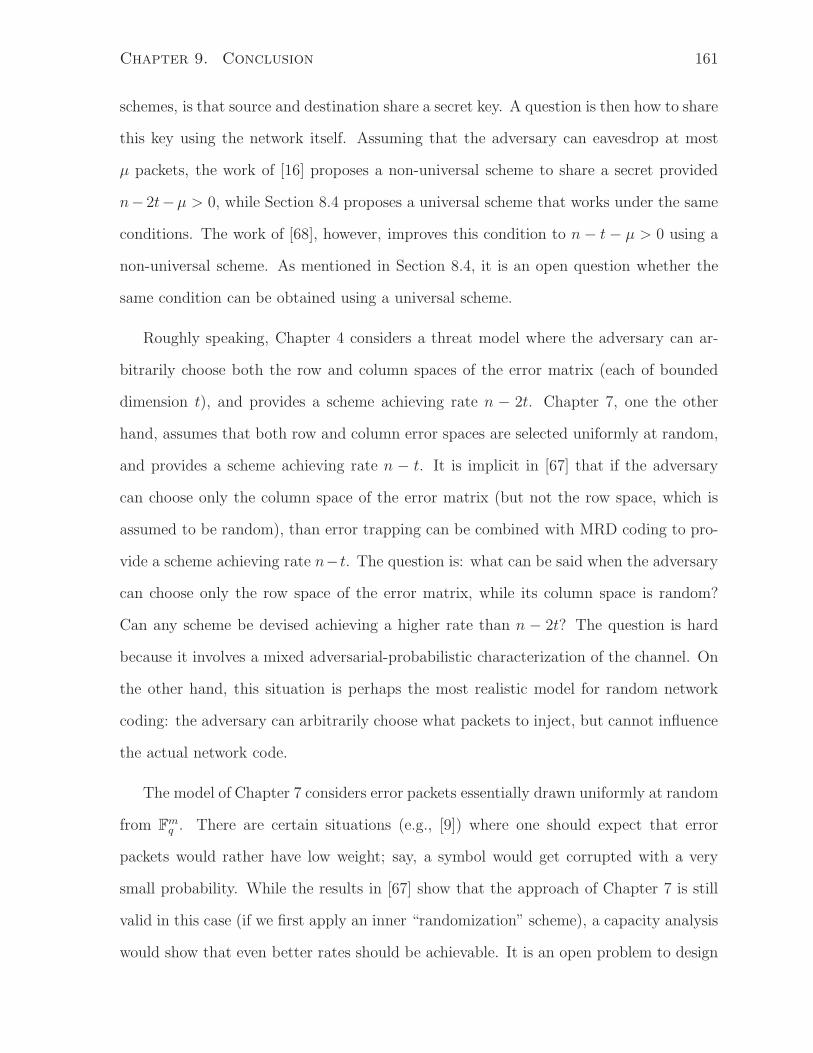
Chapter 9. Conclusion 161
schemes, is that source and destination share a secret key. A question is then how to share
this key using the network itself. Assuming that the adversary can eavesdrop at most
µ packets, the work of [16] proposes a non-universal scheme to share a secret provided
n− 2t−µ > 0, while Section 8.4 proposes a universal scheme that works under the same
conditions. The work of [68], however, improves this condition to n − t − µ > 0 using a
non-universal scheme. As mentioned in Section 8.4, it is an open question whether the
same condition can be obtained using a universal scheme.
Roughly speaking, Chapter 4 considers a threat model where the adversary can ar-
bitrarily choose both the row and column spaces of the error matrix (each of bounded
dimension t), and provides a scheme achieving rate n − 2t. Chapter 7, one the other
hand, assumes that both row and column error spaces are selected uniformly at random,
and provides a scheme achieving rate n − t. It is implicit in [67] that if the adversary
can choose only the column space of the error matrix (but not the row space, which is
assumed to be random), than error trapping can be combined with MRD coding to pro-
vide a scheme achieving rate n−t. The question is: what can be said when the adversary
can choose only the row space of the error matrix, while its column space is random?
Can any scheme be devised achieving a higher rate than n − 2t? The question is hard
because it involves a mixed adversarial-probabilistic characterization of the channel. On
the other hand, this situation is perhaps the most realistic model for random network
coding: the adversary can arbitrarily choose what packets to inject, but cannot influence
the actual network code.
The model of Chapter 7 considers error packets essentially drawn uniformly at random
from Fmq . There are certain situations (e.g., [9]) where one should expect that error
packets would rather have low weight; say, a symbol would get corrupted with a very
small probability. While the results in [67] show that the approach of Chapter 7 is still
valid in this case (if we first apply an inner “randomization” scheme), a capacity analysis
would show that even better rates should be achievable. It is an open problem to design

Chapter 9. Conclusion 162
coding schemes that are matched to these specific types of error patterns.
Another open problem, which may be specially appealing to mathematicians, is the
design of optimal subspace codes for the injection metric. Several recent results have
proposed upper and lower bounds on the size of optimal codes, as well as constructions
of codes that are superior to liftings of MRD codes. Although most of these results
consider either constant-dimension codes or general subspace codes under the subspace
metric [52, 74–78], some of the most recent ones have started considering bounds and
constructions for the injection metric [77, 79].
Another problem that might be interesting to mathematicians concerns the explicit
construction of matrices that allow weak security against the maximum number of
guesses. The proof of Theorem 8.10 not only is an existential argument (which requires
exponential design complexity [4]) but also is loose in many cases (as Proposition 8.11 ev-
idences). New algebraic tools on extensions of finite fields and corresponding linear maps
could enable the efficient design of matrices for weak security requiring much smaller
packet sizes.
Another potential research area that we might suggest concerns the efficient imple-
mentation of Gabidulin encoders and decoders—either in hardware or in GPU-based
software. As discussed in Chapter 6, the complexity bottleneck for the standard (time-
domain) Gabidulin decoder is now the Berlekamp-Massey algorithm and Gabidulin’s
algorithm. For high-rate codes, these could perhaps be efficiently implemented by “hard-
coding” the equations involved. Also, as mentioned in Section 6.6, for Cartesian-type
Gabidulin codes, the received words in the same received matrix may share the same er-
ror location patterns; exploiting this situation could significantly speed up the decoding.
In any case, we believe that parallelization, which has become commonplace in today’s
hardware and software implementations, can provide dramatic gains that are not revealed
by time-complexity expressions such as those presented in Chapter 6.

Appendix A
Detection Capability
When dealing with communication over an adversarial channel, there is little justification
to consider the possibility of error detection. In principle, a code should be designed to
be unambiguous (in which case error detection is not needed); otherwise, if there is any
possibility for ambiguity at the receiver, then the adversary will certainly exploit this
possibility, leading to a high probability of decoding failure (detected error). Still, if a
system is such that (a) sequential transmissions are made over the same channel, (b)
there exists a feedback link from the receiver to the transmitter, and (c) the adversary
is not able to fully exploit the channel, then it might be worth using a code with a lower
correction capability (but higher rate) that has some ability to detect errors.
Following classical coding theory, we consider error detection in the presence of a
bounded error-correcting decoder. More precisely, define a bounded-discrepancy decoder
with correction radius t, or simply a t-discrepancy-correcting decoder, by
x(y) =
x if ∆(x, y) ≤ t and ∆(x′, y) > t for all x′ 6= x, x′ ∈ C
f otherwise.
Of course, when using a t-discrepancy-correcting decoder we implicitly assume that the
code is t-discrepancy-correcting. The discrepancy correction capability of a code (under
a t-discrepancy-correcting decoder) is the maximum value of discrepancy for which the
163
Appendix A. Detection Capability 164
decoder above is guaranteed to return f .
For t ∈ N, let the function σt : X × X → N be given by
σt(x, x′) , miny∈Y : ∆(x′,y)
∆(x, y) − 1. (A.2)
Proposition A.1: The discrepancy-detection capability of a code C is given exactly by
σt(C). That is, under a t-discrepancy-correction decoder, any discrepancy of magnitude
s can be detected if and only if s ≤ σt(C).
Proof: Let t < s ≤ σt(C). Suppose that x ∈ X is transmitted and y ∈ Y is received,
where t < ∆(x, y) ≤ s. We will show that ∆(x′, y) > t, for all x′ ∈ C. Suppose, by way
of contradiction, that ∆(x′, y) ≤ t, for some x′ ∈ C, x′ 6= x. Then σt(C) ≤ ∆(x, y) − 1 ≤
s − 1 < s ≤ σt(C), which is a contradiction.
Conversely, assume that σt(C) < s, i.e., σt(C) ≤ s − 1. We will show that an
undetected error may occur. Since σt(C) ≤ s − 1, there exist x, x′ ∈ C such that
σt(x, x′) ≤ s − 1. This implies that there exists some y ∈ Y such that ∆(x′, y) ≤ t
and ∆(x, y) − 1 ≤ s − 1. By assumption, C is t-discrepancy-correcting, so x(y) = x′.
Thus, if x is transmitted and y is received, an undetected error will occur, even though
∆(x, y) ≤ s.
The result above has also been obtained in [50], although with a different notation
(in particular, treating σ0(x, x′) + 1 as a “distance” function). Below, we characterize
the detection capability of a code in terms of the ∆-distance.
Proposition A.2: For any code C, we have σt(C) ≥ δ(C) − t − 1.
Proof: For any x, x′ ∈ X , let y ∈ Y be a solution to the minimization in (A.2), i.e., y is
such that ∆(x′, y) ≤ t and ∆(x, y) = 1 + σt(x, x′). Then δ(x, x′) ≤ ∆(x, y) + ∆(x′, y) ≤
1 + σt(x, x′) + t, which implies that σt(x, x′) ≤ δ(x, x′) − t − 1.
Theorem A.3: Suppose that ∆(·, ·) is normal. For every code C ⊆ X , we have σt(C) =
δ(C) − t − 1.

Appendix A. Detection Capability 165
Proof: We just need to show that σt(C) ≤ δ(C)− t−1. Take any x, x′ ∈ X . Since ∆(·, ·)
is normal, there exists some y ∈ Y such that ∆(x′, y) = t and ∆(x, y) = δ(x, x′) − t.
Thus, σt(x, x′) ≤ ∆(x, y) − 1 = δ(x, x′) − t − 1.

Appendix B
Omitted Proofs
B.1 Proofs for Chapter 4
Before proving Lemma 4.15, we need the following result [27].
Lemma B.1: Let X, Y ∈ FN×Mq . Then
rank(X − Y ) ≥ maxrank X, rank Y − dim(〈X〉 ∩ 〈Y 〉).
Proof: We have
rank
X
Y
= rank
X
Y − X
≤ rank(Y − X) + rank X
rank
X
Y
= rank
Y − X
Y
≤ rank(Y − X) + rank Y.
Thus,
rank
X
Y
≤ rank(Y − X) + minrank X, rank Y .
The result now follows by applying (2.7).
166

Appendix B. Omitted Proofs 167
Proof (of Lemma 4.15): Using Lemma B.1 and (2.5), we have
rank(AX − BY ) ≥ maxrank AX, rank BY − dim(〈AX〉 ∩ 〈BY 〉)
≥ maxrank X − ρ, rank Y − σ − dim(〈X〉 ∩ 〈Y 〉).
We will now show that this lower bound is achievable. Our approach will be to
construct A as A = A1A2, where A1 ∈ FL×(L+ρ)q and A2 ∈ F
(L+ρ)×nq are both full-rank
matrices. Then (2.5) guarantees that rank A ≥ n− ρ. The matrix B will be constructed
similarly: B = B1B2, where B1 ∈ FL×(L+σ)q and B2 ∈ F
(L+σ)×Nq are both full-rank.
Let k = rank X, s = rank Y , and w = dim(〈X〉 ∩ 〈Y 〉). Let W ∈ Fw×mq be such that
〈W 〉 = 〈X〉∩〈Y 〉, let X ∈ F(k−w)×mq be such that 〈W 〉+〈X〉 = 〈X〉 and let Y ∈ F
(s−w)×mq
be such that 〈W 〉 + 〈Y 〉 = 〈Y 〉. Then, let A2 and B2 be such that
A2X =
W
X
0
and B2Y =
W
Y
0
.
Now, choose any A ∈ Fi×(k−w)q and B ∈ F
j×(s−w)q that have full row rank, where
i = [k − w − ρ]+ and j = [s − w − σ]+. For instance, we may pick A =
[
I 0
]
and
B =
[
I 0
]
. Finally, let
A1 =
I 0 0 0
0 A 0 0
0 0 I 0
and B1 =
I 0 0 0
0 B 0 0
0 0 I 0
where, in both cases, the upper identity matrix is w × w.
Appendix B. Omitted Proofs 168
We have
rank(AX − BY ) = rank(A1A2X − B1B2Y )
= rank(
W
AX
0
−
W
BY
0
)
= maxi, j
= maxk − w − ρ, s − w − σ, 0
= [maxk − ρ, s − σ − w]+ .
B.2 Proofs for Chapter 5
Before proving Proposition 5.2, note that Lemma 4.15 (together with (2.9)) implies that,
for all X ∈ Fn×mq , Y ∈ FN×m
q and Z ∈ Fn×Mq , we have
minA∈F
N×nq
rank(Y − AX) = rank
Y
X
− rank X (B.5)
minB∈F
m×Mq
rank(Z − XB) = rank
[
Z X
]
− rank X. (B.6)
Proof (of Proposition 5.2): Let
ǫ′ = minV (1),L(2)
rank(e − LV (1) − L(2)V ).
We first show the equivalence of 1) and 2). From (B.5), we have
minL(2)
rank(e − LV (1) − L(2)V ) = rank
e − LV (1)
V
− rank V .

Appendix B. Omitted Proofs 169
Similarly, from (B.6) we have
minV (1)
rank
e − LV (1)
V
= min
V (1)rank
e
V
−
L
0
V (1)
= rank
L e
0 V
− rank L.
Thus,
ǫ′ = rank
L e
0 V
− µ − δ
and the equivalence is shown.
Now, observe that the statement in 3) is equivalent to the statement that τ ∗ − µ − δ
is the minimum value of ǫ for which there exist V (1) ∈ Fµ×mq , L(2) ∈ Fn×δ
q , L(3) ∈ Fn×ǫq
and V (3) ∈ Fǫ×mq satisfying
e = LV (1) + L(2)V + L(3)V (3).
To show the equivalence of 2) and 3), we will show that ǫ′ = ǫ′′, where
ǫ′′ = minǫ,V (1),L(2),L(3),V (3):
e=LV (1)+L(2)V +L(3)V (3)
ǫ.
We can rewrite ǫ′′ as
ǫ′′ = minV (1),L(2)
minǫ,L(3),V (3):
e−LV (1)−L(2)V =L(3)V (3)
ǫ
= minV (1),L(2)
rank(e − LV (1) − L(2)V ) (B.11)
= ǫ′.
where (B.11) follows from (2.1). This shows the equivalence between 2) and 3).

Appendix B. Omitted Proofs 170
Proof (of Theorem 5.4): Let us write X =
[
I x
]
, Y =
[
A y
]
, and Z =
[
W z
]
,
where x ∈ Fn×mq , A ∈ FN×n
q , y ∈ FN×mq , W ∈ Ft×n
q , and z ∈ Ft×mq .
(=⇒) From (3.4), we have
A = A + DW and A = A − DW.
Applying (2.4) to the above equations, we obtain
rank A − t ≤ rank A ≤ rank A + t
which implies that ρ − t ≤ µ ≤ ρ + t. Similarly, observe that
Y = (A − DW )X + DZ = AX + D(Z − WX). (B.14)
Applying (2.4) to (3.4) and (B.14), it follows that
rank Y ≤ minrank A + t, rank A + t
i.e., δ = rank Y − n + µ ≤ mint − ρ + µ, t. Now, let us determine the possible values
of ǫ. From (3.4), we know that
∆ρ(X, Y ) ≤ ∆A(X, Y ) ≤ t.
Thus, according to Theorem 5.1 and Theorem 4.16,
ǫ = dI(〈X〉 , 〈Y 〉) + minµ, δ − µ − δ
= maxrank X, rank Y − dim(〈X〉 ∩ 〈Y 〉) − maxµ, δ
= maxn, n − µ + δ + ∆ρ(X, Y ) − maxn − ρ, n − µ + δ − maxµ, δ
= maxµ, δ + ∆ρ(X, Y ) − maxµ − ρ, δ − maxµ, δ
= ∆ρ(X, Y ) − maxµ − ρ, δ
≤ t − maxµ − ρ, δ.

Appendix B. Omitted Proofs 171
The remaining inequalities for µ, δ and ǫ are trivially satisfied.
(⇐=) Let us choose z = z + Wx for some z ∈ Ft×mq . From (B.14), note that y =
Ax + D(z − Wx) = A + Dz. We have
rank
X
Y
= rank
X
AX + DZ
= rank
X
DZ
= rank
I x
DW Dz
= rank
I x
0 Dz − DWx
= n + rank Dz.
Suppose that rank A = n − µ (this will be obtained later). Then there exists some
full-rank matrix T2 ∈ F(N−n+µ)×Nq such that T2A = 0. Let T1 ∈ F
(n−µ)×Nq be some matrix
such that T =
T1
T2
is nonsingular. Note that 〈T1〉 has trivial intersection with the left
null space of A. Then
TY =
T1Y
T2Y
=
T1A T1y
T2A T2y
=
T1A T1y
0 T2Dz
= rank T1A + rank T2Dz
= n − µ + rank T2Dz.

Appendix B. Omitted Proofs 172
Let A = PQ be a full-rank decomposition, where P ∈ FN×(n−ρ)q and Q ∈ F
(n−ρ)×nq . We
will now proceed to finding D, W and z such that Y = AX + DZ satisfies (5.29)–(5.31).
Two cases must be considered.
First, consider the case that µ− ρ ≥ 0. In this case, the rank of A must be decreased
by µ− ρ units when adding DW to form A. Let us write P =
[
P1 P2
]
and Q =
Q1
Q2
,
where P1 ∈ FN×(µ−ρ)q , P2 ∈ F
N×(n−µ)q , Q1 ∈ F
(µ−ρ)×nq , and Q2 ∈ F
(n−µ)×nq . Let D =
[
D1 D2 D3
]
and W =
[
W1 W2 W3
]
, where we choose
D1 = P1 W1 = −Q1
D2 ∈ FN×[δ−µ+ρ]+
q such that
[
P D2
]
is full-rank W2 = 0[δ−µ+ρ]+×n
D3 as the first t − maxµ − ρ, δ columns of P2 W3 = 0(t−maxµ−ρ,δ)×n.
Note that this is always possible according to our assumptions. Also note that the
resulting D is full-rank. It follows that
A = P1Q1 + P2Q2 + D1W1 + D2W2 + D3W3 = P2Q2.
Thus, rank A = n − µ. Moreover, since T2P2 = 0, we have
T2D = T2
[
D1 D2 D3
]
=
[
T2D1 T2D2 0
]
and, by construction, T2
[
D1 D2
]
is full-rank. Let us write z =
z1
z2
, where z1 and z2
have maxµ − ρ, δ and t − maxµ − ρ, δ rows, respectively. It follows that rank Y =
n − µ + rank z1. By choosing z1 with rank δ and z2 such that rank z = δ + ǫ (which is
possible according to our assumptions), we obtain the desired result.
Now, let us consider the case that ρ − µ ≥ 0. In this case, the addition of DW
should have the effect of increasing the rank of A by ρ − µ units. As before, let D =

Appendix B. Omitted Proofs 173
[
D1 D2 D3
]
and W =
[
W1 W2 W3
]
, but now choose
D1 ∈ FN×(ρ−µ)q such that
[
P D1
]
is full-rank
W1 ∈ F(ρ−µ)×nq such that
Q
W1
is full-rank
D2 ∈ FN×δq such that
[
D1 D2
]
is full-rank
W2 = 0δ×n
D3 as the first t − δ − ρ + µ columns of P
W2 = 0(t−δ−ρ+µ)×n.
Note that this is always possible according to our assumptions. It follows that
A = PQ + D1W1 + D2W2 + D3W3 =
[
P D1
]
Q
W1
.
Thus, rank A = n − µ. Moreover, since T2
[
P D1
]
= 0, we have
T2D = T2
[
D1 D2 D3
]
=
[
0 T2D2 0
]
and, by construction, T2D2 is full-rank. Let us write z =
z1
z2
z3
, where z1, z2, z3 have
ρ − µ, δ, and t − δ − ρ + µ rows, respectively. It follows that rank Y = n − µ + rank z2.
By choosing z2 with rank δ and z1 and z3 such that rank z = δ + ǫ (which is possible
according to our assumptions), we obtain the desired result.

Appendix B. Omitted Proofs 174
B.3 Proofs for Chapter 8
Proof (of Proposition 8.1): To prove 1), let W = Bx : x ∈ F n and
Xs,w =
x ∈ F n :
s
w
=
H
B
x
.
Observe that
H(W ) ≤ log|F | |W| = rank B
H(X|S) = log|F | |XS| = dim ker(H) = n − rank H
H(X|S, W ) ≤ log|F | |XS,W | = n − rank
H
B
.
From (8.3), it follows that
I(S; W ) ≤ rank H + rank B − rank
H
B
.
Now, to prove 2), first note that
dim(〈H〉 ∩ 〈B〉) = rank
H
B
− rank H − rank B.
Suppose dim(〈H〉 ∩ 〈B〉) = t > 0. Then there exist full-rank matrices T1 ∈ F t×µ and
T2 ∈ F t×k such that T1B = T2H . This implies that
T1W = T1BX = T2HX = T2S.
Since S is uniform, we have that I(S; W ) ≥ t > 0.
Proof (of Lemma 8.4): Assume I(S; W ) = 0. Using (8.3), it follows that
H(X|S, W ) = H(X|S) − H(W ).

Appendix B. Omitted Proofs 175
We will now show that H(W ) − H(X|S) ≥ 0, which implies that H(X|S, W ) = 0.
We have
H(W ) − H(X|S) = E[− log pW (W ) + log pX|S(X|S)
]
= E
[
logpX|S(X|S)
pW (W )
]
= E
[
logpS|X(S|X)pX(X)
pW (W )pS(S)
]
= E
[
logpS|X(f(X)|X)pX(X)
pW (g(X))pS(f(X))
]
= E
[
logpX(X)
pW (g(X))pS(f(X))
]
= D(pX(x) ‖ pW (g(x))pS(f(x))
)
where D(· ‖ ·) denotes the relative entropy [64].
It remains to prove that pW (g(x))pS(f(x)) is indeed a probability mass function on
X , i.e., that∑
x∈X
pW (g(x))pS(f(x)) = 1. (B.26)
Then the result will follow from the nonnegativity of the relative entropy.
Since S is uniform, we have that pS(f(x)) = 1/|S|, ∀x. Moreover,
∑
x∈X
pW (g(x)) =∑
w∈W
∑
x∈X :g(x)=w
pW (g(x))
=∑
w∈W
pW (w)∑
x∈X :g(x)=w
1
=∑
w∈W
pW (w) |x ∈ X : g(x) = w|
= |S|.
Thus, (B.26) holds and the proof is complete.
Bibliography
[1] M. Effros, R. Koetter, and M. Medard, “Breaking network logjams,” Scientific
American, vol. 6, pp. 78–85, Jun. 2007.
[2] R. Ahlswede, N. Cai, S.-Y. R. Li, and R. W. Yeung, “Network information flow,”
IEEE Trans. Inf. Theory, vol. 46, no. 4, pp. 1204–1216, Jul. 2000.
[3] S.-Y. R. Li, R. W. Yeung, and N. Cai, “Linear network coding,” IEEE Trans. Inf.
Theory, vol. 49, no. 2, pp. 371–381, Feb. 2003.
[4] R. Koetter and M. Medard, “An algebraic approach to network coding,” IEEE/ACM
Trans. Netw., vol. 11, no. 5, pp. 782–795, Oct. 2003.
[5] T. Ho, R. Koetter, M. Medard, D. R. Karger, and M. Effros, “The benefits of coding
over routing in a randomized setting,” in Proc. IEEE Int. Symp. Information Theory,
Yokohama, Japan, Jun. 29–Jul. 4, 2003, p. 442.
[6] T. Ho, M. Medard, R. Koetter, D. R. Karger, M. Effros, J. Shi, and B. Leong, “A
random linear network coding approach to multicast,” IEEE Trans. Inf. Theory,
vol. 52, no. 10, pp. 4413–4430, Oct. 2006.
[7] L. L. Peterson and B. S. Davie, Computer Networks: A Systems Approach, 4th ed.
San Francisco, CA: Morgan Kaufmann, 2007.
[8] “The network coding homepage.” [Online]. Available:
http://www.ifp.uiuc.edu/ koetter/NWC/Bibliography.html
176

Bibliography 177
[9] S. Katti, D. Katabi, H. Balakrishnan, and M. Medard, “Symbol-level network coding
for wireless mesh networks,” in ACM SIGCOMM, Seattle, WA, Aug. 2008.
[10] N. Cai and R. W. Yeung, “Network coding and error correction,” in Proc. 2002
IEEE Inform. Theory Workshop, Bangalore, India, Oct. 20–25, 2002, pp. 119–122.
[11] R. W. Yeung and N. Cai, “Network error correction, part I: Basic concepts and
upper bounds,” Commun. Inform. Syst., vol. 6, no. 1, pp. 19–36, 2006.
[12] N. Cai and R. W. Yeung, “Network error correction, part II: Lower bounds,” Com-
mun. Inform. Syst., vol. 6, no. 1, pp. 37–54, 2006.
[13] Z. Zhang, “Network error correction coding in packetized networks,” in Proc. 2006
IEEE Inform. Theory Workshop, Chengdu, China, Oct. 22–26, 2006, pp. 433–437.
[14] ——, “Linear network error correction codes in packet networks,” IEEE Trans. Inf.
Theory, vol. 54, no. 1, pp. 209–218, 2008.
[15] S. Jaggi, M. Langberg, S. Katti, T. Ho, D. Katabi, and M. Medard, “Resilient
network coding in the presence of Byzantine adversaries,” in Proc. 26th IEEE Int.
Conf. on Computer Commun., Anchorage, AK, May 2007, pp. 616–624.
[16] S. Jaggi, M. Langberg, S. Katti, T. Ho, D. Katabi, M. Medard, and M. Effros,
“Resilient network coding in the presence of Byzantine adversaries,” IEEE Trans.
Inf. Theory, vol. 54, no. 6, pp. 2596–2603, Jun. 2008.
[17] R. Koetter and F. R. Kschischang, “Coding for errors and erasures in random net-
work coding,” in Proc. IEEE Int. Symp. Information Theory, Nice, France, Jun.
24–29, 2007, pp. 791–795.
[18] R. Kotter and F. R. Kschischang, “Coding for errors and erasures in random network
coding,” IEEE Trans. Inf. Theory, vol. 54, no. 8, pp. 3579–3591, Aug. 2008.

Bibliography 178
[19] L. H. Ozarow and A. D. Wyner, “Wire-tap channel II,” in Proc. EUROCRYPT 84
workshop on Advances in cryptology: theory and applicationof cryptographic tech-
niques. New York, NY, USA: Springer-Verlag New York, Inc., 1985, pp. 33–51.
[20] N. Cai and R. W. Yeung, “Secure network coding,” in Proc. IEEE Int. Symp. In-
formation Theory, Lausanne, Switzerland, Jun. 30–Jul. 5, 2002, p. 323.
[21] J. Feldman, T. Malkin, C. Stein, and R. A. Servedio, “On the capacity of secure
network coding,” in Proc. 42nd Annual Allerton Conf. on Commun., Control, and
Computing, Sep. 2004.
[22] S. Y. E. Rouayheb and E. Soljanin, “On wiretap networks II,” in Proc. IEEE Int.
Symp. Information Theory, Nice, France, Jun. 24–29, 2007, pp. 551–555.
[23] A. Montanari and R. Urbanke, “Iterative coding for network coding,” 2007,
submitted for publication. [Online]. Available: http://arxiv.org/abs/0711.3935
[24] K. Bhattad and K. R. Narayanan, “Weakly secure network coding,” in Proc. NetCod
2005, Riva del Garda, Italy, Apr. 2005.
[25] D. Silva and F. R. Kschischang, “Using rank-metric codes for error correction in ran-
dom network coding,” in Proc. IEEE Int. Symp. Information Theory, Nice, France,
Jun. 24–29, 2007, pp. 796–800.
[26] D. Silva, F. R. Kschischang, and R. Koetter, “A rank-metric approach to error
control in random network coding,” in Proc. IEEE Information Theory Workshop
on Information Theory for Wireless Networks, Bergen, Norway, Jul. 1–6, 2007.
[27] D. Silva, F. R. Kschischang, and R. Kotter, “A rank-metric approach to error control
in random network coding,” IEEE Trans. Inf. Theory, vol. 54, no. 9, pp. 3951–3967,
2008.
Bibliography 179
[28] D. Silva and F. R. Kschischang, “Adversarial error correction for network coding:
Models and metrics,” in Proc. 46th Annual Allerton Conf. on Commun., Control,
and Computing, Monticello, IL, Sep. 23-26, 2008, pp. 1246–1253.
[29] ——, “On metrics for error correction in network coding,” IEEE Trans. Inf.
Theory, 2008, to be published. [Online]. Available: http://arxiv.org/abs/0805.3824
[30] ——, “Fast encoding and decoding of Gabidulin codes,” in Proc. IEEE Int. Symp.
Information Theory, Seoul, Korea, Jun. 28–Jul. 3, 2009, pp. 2858–2862.
[31] D. Silva, F. R. Kschischang, and R. Kotter, “Capacity of random network coding
under a probabilistic error model,” in Proc. 24th Biennial Symp. Communications,
Kingston, Ontario, Canada, Jun. 24–26, 2008, pp. 9–12.
[32] ——, “Communication over finite-field matrix channels,” IEEE Trans. Inf. Theory,
2008, to be published. [Online]. Available: http://arxiv.org/abs/0807.1372
[33] D. Silva and F. R. Kschischang, “Security for wiretap networks via rank-metric
codes,” in Proc. IEEE Int. Symp. Information Theory, Toronto, Canada, Jul. 6–11,
2008, pp. 176–180.
[34] ——, “Universal weakly secure network coding,” in Proc. Inform. Theory Workshop
on Networking and Inform. Theory, Volos, Greece, Jun. 10-12, 2009, pp. 281–285.
[35] ——, “Universal secure network coding via rank-metric codes,” IEEE
Trans. Inf. Theory, 2008, submitted for publication. [Online]. Available:
http://arxiv.org/abs/0809.3546
[36] A. R. Rao and P. Bhimasankaram, Linear Algebra, 2nd ed. New Delhi, India:
Hindustan Book Agency, 2000.
[37] E. M. Gabidulin, “Theory of codes with maximum rank distance,” Probl. Inform.
Transm., vol. 21, no. 1, pp. 1–12, 1985.
Bibliography 180
[38] R. Lidl and H. Niederreiter, Finite Fields. Reading, MA: Addison-Wesley, 1983.
[39] S. H. Friedberg, A. J. Insel, and L. E. Spence, Linear Algebra, 4th ed. Upper Saddle
River, NJ: Prentice Hall, 2003.
[40] R. M. Roth, “Maximum-rank array codes and their application to crisscross error
correction,” IEEE Trans. Inf. Theory, vol. 37, pp. 328–336, 1991.
[41] P. Delsarte, “Bilinear forms over a finite field, with applications to coding theory,”
J. of Comb. Theory. Series A, vol. 25, pp. 226–241, 1978.
[42] P. Loidreau, “Etude et optimisation de cryptosystemes a cle publique fondes sur
la theorie des codes correcteurs,” Ph.D. Dissertation, Ecole Polytechnique, Paris,
France, May 2001.
[43] M. Gadouleau and Z. Yan, “Packing and covering properties of rank metric codes,”
IEEE Trans. Inf. Theory, vol. 54, no. 9, pp. 3873–3883, 2008.
[44] S. Gao, “Normal bases over finite fields,” Ph.D. dissertation, University of Waterloo,
Department of Combinatorics and Optimization, 1993.
[45] S. Gao, J. von zur Gathen, D. Panario, and V. Shoup, “Algorithms for exponentia-
tion in finite fields,” J. Symbolic Computation, vol. 29, pp. 879–889, 2000.
[46] J. von zur Gathen and J. Gerhard, Modern Computer Algebra, 2nd ed. New York:
Cambridge University Press, 2003.
[47] P. A. Chou, Y. Wu, and K. Jain, “Practical network coding,” in Proc. Allerton Conf.
on Comm., Control, and Computing, Monticello, IL, Oct. 2003, pp. 40–49.
[48] S. Yang and R. W. Yeung, “Characterizations of network error correction/detection
and erasure correction,” in Proc. NetCod 2007, San Diego, CA, Jan. 2007.
Bibliography 181
[49] S. Jaggi, P. Sanders, P. Chou, M. Effros, S. Egner, K. Jain, and L. Tolhuizen,
“Polynomial time algorithms for multicast network code construction,” IEEE Trans.
Inf. Theory, vol. 51, no. 6, pp. 1973–1982, Jun. 2005.
[50] S. Yang, R. W. Yeung, and Z. Zhang, “Weight properties of network codes,” Euro-
pean Transactions on Telecommunications, vol. 19, no. 4, pp. 371–383, 2008.
[51] S. Yang and R. W. Yeung, “Refined coding bounds for network error correction,”
in Proc. 2007 IEEE Information Theory Workshop, Bergen, Norway, Jul. 1–6, 2007,
pp. 1–5.
[52] S.-T. Xia and F.-W. Fu, “Johnson type bounds on constant dimension codes,” De-
signs, Codes and Cryptography, vol. 50, no. 2, pp. 163–172, Feb. 2009.
[53] H. Wang, C. Xing, and R. Safavi-Naini, “Linear authentication codes: bounds and
constructions,” IEEE Trans. Inf. Theory, vol. 49, no. 4, pp. 866–872, 2003.
[54] E. M. Gabidulin, A. V. Paramonov, and O. V. Tretjakov, “Rank errors and rank
erasures correction,” in Proc. 4th Int. Colloq. Coding Theory, Dilijan, Armenia,
1991, Yerevan, 1992, pp. 11–19.
[55] E. M. Gabidulin and N. I. Pilipchuk, “A new method of erasure correction by rank
codes,” in Proc. IEEE Int. Symp. Information Theory, Jun. 29–Jul. 4, 2003, p. 423.
[56] G. Richter and S. Plass, “Error and erasure decoding of rank-codes with a modified
Berlekamp-Massey algorithm,” in Proc. ITG Conf. on Source and Channel Coding,
Erlangen, Germany, Jan. 2004, pp. 249–256.
[57] ——, “Fast decoding of rank-codes with rank errors and column erasures,” in Proc.
IEEE Int. Symp. Information Theory, Jun. 27–Jul. 2, 2004, pp. 398–398.

Bibliography 182
[58] E. M. Gabidulin and N. I. Pilipchuk, “Error and erasure correcting algorithms for
rank codes,” Designs, Codes and Cryptography, vol. 49, no. 1-3, pp. 105–122, Dec.
2008.
[59] R. E. Blahut, “Transform techniques for error control codes,” IBM J. Res. Develop.,
vol. 23, pp. 299–315, May 1979.
[60] ——, Algebraic codes for data transmission. Cambridge, UK: Cambridge Univ.
Press, 2003.
[61] V. Skachek and R. M. Roth, “Probabilistic algorithm for finding roots of linearized
polynomials,” Designs, Codes and Cryptography, vol. 46, no. 1, pp. 17–23, 2008, also
in Comput. Sci. Dept., Technion, Tech. Rep. CS-2004-08, Jun. 2004.
[62] E. R. Berlekamp, Algebraic Coding Theory. New York: McGraw-Hill, 1968.
[63] M. Gadouleau and Z. Yan, “Complexity of decoding Gabidulin codes,” in Proc.
Annual Conf. Inform. Sciences and Syst., Princeton, NJ, Mar. 19–21, 2008, pp.
1081–1085.
[64] T. M. Cover and J. A. Thomas, Elements of Information Theory. John Wiley &
sons, 1991.
[65] M. Siavoshani, C. Fragouli, and S. Diggavi, “Noncoherent multisource network cod-
ing,” in Proc. IEEE Int. Symp. Information Theory, Toronto, Canada, Jul. 6–11,
2008, pp. 817–821.
[66] D. S. Dummit and R. M. Foote, Abstract Algebra, 3rd ed. John Wiley & Sons,
2004.
[67] D. Silva and F. R. Kschischang, “A key-based error control scheme for network
coding,” in Proc. 11th Canadian Workshop Inform. Theory, Ottawa, Canada, May
13-15, 2009, pp. 5–8.

Bibliography 183
[68] S. Jaggi and M. Langberg, “Resilient network codes in the presence of eavesdropping
Byzantine adversaries,” in Proc. IEEE Int. Symp. Information Theory, 24–29 June
2007, pp. 541–545.
[69] R. G. Gallager, Principles of Digital Communication. Cambridge, UK: Cambridge
Univ. Press, 2008.
[70] A. Albanese, J. Blomer, J. Edmonds, M. Luby, and M. Sudan, “Priority encoding
transmission,” IEEE Trans. Inf. Theory, vol. 42, no. 6, pp. 1737–1744, Nov. 1996.
[71] D. Silva and F. R. Kschischang, “Rank-metric codes for priority encoding trans-
mission with network coding,” in Proc. 10th Canadian Workshop Inform. Theory,
Edmonton, Alberta, Canada, Jun. 6–8, 2007, pp. 81–84.
[72] R. W. Nobrega and B. F. Uchoa-Filho, “Multishot codes for network coding: Bounds
and a multilevel construction,” in Proc. IEEE Int. Symp. Information Theory, Seoul,
Korea, Jun. 28–Jul. 3, 2009, pp. 428–432.
[73] L. Nutman and M. Langberg, “Adversarial models and resilient schemes for network
coding,” in Proc. IEEE Int. Symp. Information Theory, Toronto, Canada, Jul. 6–11,
2008, pp. 171–175.
[74] T. Etzion and N. Silberstein, “Error-correcting codes in projective spaces via rank-
metric codes and Ferrers diagrams,” IEEE Trans. Inf. Theory, vol. 55, no. 7, pp.
2909–2919, July 2009.
[75] T. Etzion and A. Vardy, “Error-correcting codes in projective space,” in Proc. IEEE
Int. Symp. Information Theory, Toronto, Canada, Jul. 6–11, 2008, pp. 871–875.
[76] A. Kohnert and S. Kurz, “Construction of large constant dimension codes with a
prescribed minimum distance,” Lecture Notes in Computer Science, vol. 5393, pp.
31–42, 2008.

Bibliography 184
[77] M. Gadouleau and Z. Yan, “Packing and covering properties of subspace codes,” in
Proc. IEEE Int. Symp. Information Theory, Seoul, Korea, Jun. 28–Jul. 3, 2009, pp.
2867–2871.
[78] ——, “Construction and covering properties of constant-dimension codes,” in Proc.
IEEE Int. Symp. Information Theory, Seoul, Korea, Jun. 28–Jul. 3, 2009, pp. 2221–
2225.
[79] A. Khaleghi and F. R. Kschischang, “Projective space codes for the injection metric,”
in Proc. 11th Canadian Workshop Inform. Theory, Ottawa, Canada, May 13–15,
2009, pp. 9–12.


