83050/334

ERROR CONTROL CODING _________________________________________________ During transmission in non-ideal channels, some bits are changed and received with errors. It is a very important task to handle those errors properly in the receiver. Therefore, error detection and/or error correction are used in all practical digital transmission systems to increase the reliability. These methods help in exploiting the channel capacity in an efficient way with increased reliability. The basics of error control coding are presented in this part of lecture notes. This is very important and very wide area. In the next slides, only the basic principles of some important coding methods are considered and their importance to digital the transmission system is highlighted. This part covers the following topics:

- error handling methods - hard/soft decoding - block codes - convolution codes - trellis codes

Source: Lee& Messerschmitt, Chapter 11.

83050/335

Error Handling Methods _________________________________________________

The error handling task is done by channel coding, before line coding. Two different approaches exist: • Error detection: The code can be designed such it

detects, for example, all single bit-errors. After an error is detected using error detection code, the receiver requests retransmission of the part of signal which is received with errors. Error detection can be used in combination with service monitoring. • Error correction: This class of codes detect and correct

detected transmission error using redudancy.

All coding methods are based on adding some redudancy into the signal.

- The first way to add redudancy is to insert additional symbols to the transmitted symbol stream, which will also increase the symbol rate.

- The second approach is to increase the number of symbols in the alphabet while keeping the symbol rate the same.

83050/336

Hard/Soft Decoding _________________________________________________

Hard decoding

In this case, the slicer makes a ”hard decision”, in order to detect the transmitted symbols (complete with their redudancy). From the perspective of the decoder, the channel is binary and makes transmission errors, a binary symmetric channel (BSC) model can be used. Soft decoder

In this case, the decoder makes decisions on the information bits without making intermediate decisions about transmitted symbols. Soft decoding eliminates the use of a slicer. Soft decoding gives better performance at the expense of implementation complexity, because it makes use of the information that the slicer throws away.

83050/337

Classes of Codes _________________________________________________ Block codes Blocks of k source bits are mapped into blocks of n coded bits, thus n-k bits are added. The block code has a code rate k/n<1. Block codes are usually used with hard decoding, but soft decoding may also be possible. Convolutional codes Redudancy is added without dividing the source bits into blocks, in a continuos manner; the coded bits are produced at higher rate. They can be used with either hard decoding or soft decoding. Trellis codes (signal space codes) Redudancy is added, for example, by using 64-QAM constellation for 16 symbol source alphabet. It is used only with soft decoding.

83050/338

Purpose of Coding (from Benedetto&Biglieri) _________________________________________________

Here A, B and C correspond to uncoded, soft-decoding, and hard-decoding cases, respectively.

83050/339

Coding Gain _________________________________________________ In the Lee-Messerschmitt book, coding gain is defined as the reduction (in dB’s) of the required SNR to achive a given bit error rate (BER). Block codes and convolutional codes with error correction capabilities add a considerable amount of redudancy. They increase the symbol rate and required bandwith, if the line-coding and modulation method is unchanged. Consequently, in the case of AWGN channel, the noise bandwidth is also increased, and thus the SNR becomes worse if the signal power is the same. This has an effect on the useful coding gain. For trellis codes, the noise bandwidth does not change, and here the coding gain tells directly how much the transmitted signal power can be decreased due to coding.

83050/340

About the Concept of Coding Gain _________________________________________________ In the Lee-Messerschmitt book, coding gain is defined based on the SNR, and when using this definition, one has always to pay attention to the effect of increased (noise) bandwidth, resulting in reduced SNR, when evaluating the benefit of coding.

In other literature, coding gain is quite often defined using the Eb/No ratio, and the resulting coding gain tells the true benefit of the code. In this context, it is important to note that Eb is the energy in the signal corresponding to one source bit. For a rate R code, one source bit energy is 1/R times the channel bit energy. With these definitions, the BER in uncoded (u) and coded (c) cases are the same iff (see examples later)

uuubu

ccbc

c SNRWNrE

WNRrE

dSNRd ===00

2min

2min

which is equivalent to

002min // NENERd bubc =

because for fixed constellation and modulation parameters, the ratio of bit-rate and bandwidth is constant. Thus we obtain:

Coding gain = )(10log10 2minRd

which takes automatically into account the effects of different noise bandwidths.

83050/341

Block Codes _________________________________________________

(n, k)-code representation: k source bits n coded bits. A parity check code is fully characterized by its generator matrix, G:

c bG=

where is row vector of source bits b c is row vector of coded bits (codeword) G is generator matrix, consisting of zeros and ones. A code is set of all possible codewords. Every codeword is a modulo two summation of the rows of the generator matrix.

=> The zero vector is a codeword. The modulo-2 sum of any two codewords is also codeword.

The code is systematic if the k first bits of the codeword are exactly the source bits. The generator matrix of a systematic code has the following form:

G I P= k

Here Ik is k k× identity matrix. All parity check codes are linear and all linear block codes are parity check codes with some generator matrix. All linear block codes are also equivalent to a systematic code, obtained by reordering the coded bits.

83050/342

Block Codes - Example I _________________________________________________ A simple parity check code (n, n-1) (or (k+1, k))

C B C B C B

C C B B B

k k

n k

( ) ( ) ( ) ( ) ( ) ( )

( ) ( ) ( ) ( ) ( )

, , ,1 1 2 2

1 1 2

= = =

= = ⊕ ⊕ ⊕+ k

Symbol ⊕ means modulo-2 sum (exclusive-or). An extra bit is appended to ensure that there is an even number of ones in the codeword. The generator matrix is:

⎥⎥⎥⎥⎥

⎦

⎤

⎢⎢⎢⎢⎢

⎣

⎡

=

1100

10101001

G

This code is systematic. ----------------------------------- (For later reference:) The minimum Hamming weight = minimum Hamming-distance = 2 The minimum Euclidean distance is d aE = 2 2 .

83050/343

Block Codes - Example II _________________________________________________ (7,4) Hamming-code:

⎥⎥⎥⎥⎥

⎦

⎤

⎢⎢⎢⎢⎢

⎣

⎡

=

1101000011010011100101010001

G

The code is systematic. ----------------------------------- (For later reference:) Minimum Hamming-distance = 3 Minimum Euclidean distance is d aE = 2 3

83050/344

Hamming and Euclidean Distance _________________________________________________ The decoding principle can be based on the following: Choose the codeword that is closest to the received one based on:

• Euclidean distance for soft decoding • Hamming distance hard decoding.

The probability of error is dominated by the two codewords closest in Euclidean or Hamming distance measure. In the following, the important thing to remember is fact the soft decoding is superior. This comparison assumes that binary antipodal signalling is used. In this case the relation between Euclidean and Hamming distances can be expressed as: HE dad 2= In the case of linear code )(min

0

min, c

cc

HC

H wd

≠∈

=

where wH ( )c is codeword’s Hamming-weight, i.e., the number of 1- bits.

83050/345

n

Performance of Soft Decoders _________________________________________________ The input to the soft decoder is the sample stream before applying it to any slicer. Assume the AWGN case and zero ISI, and binary antipodal symbols. The observation vector is q a= +

where a is a vector of antipodal symbols that corresponds to the binary codeword c. n is vector noise samples. And the noise is white Gaussian with zero mean and variance . σc

2

As discussed earlier, an ML detector selects the vector closest to the observation q in Euclidean distance, and the following is satisfied:

( ) [ ]⎥⎥⎦

⎤

⎢⎢⎣

⎡≥≥

⎥⎥⎦

⎤

⎢⎢⎣

⎡−

c

E

c

Ek dQerrorblock

dQ

σσ 2Pr

212 min,min,

where d is minimum Euclidean distance of the code. E,min This equation shows the bounds for the probability of error in soft ML-based detection. The coarse upper bound is obtained by using union bound and assuming that all the codewords are at the minimum distance from each other. The lower bound is obtained by assuming that there is only one codeword at the the minimum distance from every codeword.

83050/346

Soft Decoding of Block Codes: Coding Gain _________________________________________________ Each block error will produce at least one bit error so we can write:

Pr , Pr ,

Pr ,

block error soft decoding bit error soft decoding

kblock error soft decoding

≥

≥1

resulting in

( ) [ ]

⎥⎥⎦

⎤

⎢⎢⎣

⎡≥≥

⎥⎥⎦

⎤

⎢⎢⎣

⎡−

c

E

c

Ek dQ

kdecodingsofterrorbit

dQ

σσ 21,Pr

212 min,min,

The uncoded system has the following bit error probability:

[ ]⎥⎥⎦

⎤

⎢⎢⎣

⎡=

u

aQsystemuncodederrorbitσ

,Pr

where is the noise variance at the slicer input for the uncoded system.

σu2

In general . σ σu c

2 2≠

83050/347

Example I: Coding Gain _________________________________________________ We consider here the simple parity check code (n, n−1). We make an approximation and use the multipler 1 for the Q function when calculating the probability of error. We require the same probability of error in coded and uncoded systems:

⎥⎥⎦

⎤

⎢⎢⎣

⎡=

⎥⎥⎦

⎤

⎢⎢⎣

⎡=

⎥⎥⎦

⎤

⎢⎢⎣

⎡

u

u

c

c

c

E aQaQd

Qσσσ 2

22

2min,

where antipodal signal with amplitudes and in uncoded and coded cases, respectively. To get the same error rates, the amplitudes should be chosen to satisfy:

ua ca

uucc aa σσ //2 = or SNR . So there is 3 dB difference in the required SNRs. SNRu = 2 c This is not the whole story. We have to take into account the larger bandwidth due to increased symbol rate by n n/ ( )−1 times. Because of this, the noise is increased. Requiring the same performance again:

σ σc u

c

u

nn

aa

nn

2 2

2

2

1

0 51

=−

=−

.

In the case when n = 3, the required signal level is 1.25 dB smaller compared to the uncoded case. The coding gain in this case is 1.25 dB, not 3 dB, because of increased noise bandwidth. (The same result can be obtained using the ideas mentioned on page 340.)

83050/348

Example I: Coding Gain (cont.) _________________________________________________ The lower and upper bounds for bit error probability are:

[ ]

( )⎥⎥⎦

⎤

⎢⎢⎣

⎡ −−≤

≤⎥⎥⎦

⎤

⎢⎢⎣

⎡ −−

−

u

n

u

nnaQ

decodingsofterrorbitnna

Qn

σ

σ

/)1(212

,Pr/)1(2

11

1

For a given probability of error, it is possible to find the power advantage numerically coresponding to the lower bound, upper bound, and crude approximation where the coefficient of the Q-function is ignored: Probability- Best worst ignoring of error case case constant ================================== 10 1.56 dB 0.77 dB 1.25 dB 5−

10 1.45 dB 0.91 dB 1.25 dB 7−

The bounds get closer as SNR increases.

83050/349

Example II: Coding Gain _________________________________________________ In this case, the minimum Hamming distance is 3, that is

[ ]

⎥⎥⎦

⎤

⎢⎢⎣

⎡≤≤

⎥⎥⎦

⎤

⎢⎢⎣

⎡

=

cc

E

aQdecodingsofterrorbitaQ

ad

σσ315,Pr3

41

32min,

The reduction in the required SNR is 10 3 4 710log .= dB. If the increase when the noise bandwidth is taken into account:

[ ] ⎥

⎦

⎤⎢⎣

⎡≤≤

⎥⎥⎦

⎤

⎢⎢⎣

⎡

=

uu

uc

aQdecodingsofterrorbitaQσσ

σσ

7/1215,Pr7/1241

47 22

Ignoring the constant in front of the Q-function, the coding gain becomes:

10 127

2 3410log .= dB

and the bounds are: Probability best worst ignoring of error case case constant ================================== 10 3.00 dB 1.25 dB 2.34 dB 5−

10 2.79 dB 1.56 dB 2.34 dB 7−

83050/350

Hard Decoding of Block Codes _________________________________________________ In a hard decoder, the decoding is done after the slicer. The equivalent binary channel model (from the decoder point of view) is usually a BSC with probability of error p. A hard-decoding ML-detector selects the codeword closest in Hamming distance to the observation. All received bit vectors having at most

( )⎣ ⎦ ⎣ ⎦ 0) towardsroundingfor stands ( min, 2/1−= Hdt

errors can be correctly decoded. The code can correct t errors per block. A perfect code has the following properties:

- all bit patterns of length n are within Hamming distance t of a codeword, and

- no bit pattern of length n is at Hamming distance t or less from more than one code word.

Practically, this means that a perfect code can detect and correct t error bits per block. Example 1: d tH,min = ⇒ =2 0 The code cannot correct any error.

83050/351

Hard Decoding of Block Codes (cont.) _________________________________________________ Example 2: d tH,min = ⇒ =3 1

The code can correct any single bit error in a codeword. (7,4) Hamming code is perfect: • All seven-bit patterns are either codewords or at one bit distance

from exactly one codeword. • Consequently, if a codeword is transmitted and two bit errors

occur, then the received codeword will be at the distance of one from another codeword. Therefore, decoding error occurs.

For example: Sent codeword: c = 0000000 Received bit vector: c = 0001010 Decoded codeword: 0001011ˆ =c

83050/352

Hard Decoding of Block Codes (cont.) _________________________________________________ Perfect codes are optimal for BSC in the sense that they minimize the probability of error among all codes with the same n and k. With independent noise components, as in BSC model, the probability of m errors in a block of n bits is calculated using the binomial distribution:

mnm ppmn

nmP −−⎟⎠

⎞⎜⎝

⎛= )1(),(

A block error occurs if more than t bit are in error:

[ ] ∑∑=+=

−==t

m

n

tmnmPnmPerrorblock

01),(1),(Pr

This relation is exact for perfect codes, for non-perfect codes we can estimate an upper bound based on this relation (in this case some error patterns with more that t bits can corrected using ML decoding). Some practical codes are quasiperfect, meaning that they could correct t+1 errors (sometimes) but not t+2 errors. The following lower bound is obtained for this case:

[ ] ∑∑+=+=

≤≤n

tm

n

tmnmPerrorblocknmP

12),(Pr),(

In the literature, many different bounds are presented for the performance of error control codes. Many of them are tighter than the ones presented above.

As seen from the results, it should be remembered that the soft decoding has a power advantage of 1-2 dB compared to hard decoding.

83050/353

Hard Decoding of Block Codes: Example _________________________________________________ Example 2: (7,4) Hamming-code Pr ( ) ( )block error p p p= − − − −1 1 7 17 6 p block error= ⇒ =0 01 0 002. Pr .

In the case of AWGN-channel σc2 7

4= σu

2, and the BSC error

probability is larger than in the uncoded system with the same input levels. The power advantage due to this kind of coding is only a fraction of dB.

83050/354

Parity Check Matrix _________________________________________________ As it was said, soft and hard ML decoders find the closest codewords (in Euclidean or Hamming distance) to the received block. For large k and n this becomes difficult (there are 2k distances to compare). For soft decoding, there are no other practical approaches, and thus they are usually impractical for large block sizes. Soft decoding is used mostly with convolution codes. For hard decoding, there are some more efficient techniques. The idea is to use codes with certain algebraic structure which can be exploited in the decoding. Here just the basic ideas are illustrated, a more complete discussion of error control coding from algebraic point of view is available in the course Coding Theory offered by the Institute of Mathematics. The generator matrix of a systematic code (n,k) has the following structure G I P= k

The codeword can be obtained as: c bG b a= = where b is source k-bit vector to be coded a are n k− parity check bits The following can be shown:

[ ]

[ ]kn

kn

−

−′==′

=⎥⎦

⎤⎢⎣

⎡

=⊕⇒=

IPH0Hc

0I

Pab

0abPbPa

,

The matrix H is called parity check matrix.

83050/355

)

Example _________________________________________________ Example 1: ( ,k k+1 parity check code. The parity check matrix is: [ ]1111=H Example 2: (7,4) Hamming-code

⎥⎥⎥

⎦

⎤

⎢⎢⎢

⎣

⎡=

100101101011100010111

H

For example c1 0= 1 1 0 0 0 1 is codeword because:

. c H 01 ′ = The vector c2 0= 1 1 0 1 0 1 is not codeword because: c H2 1′ = 0 0 . The parity check matrix can be used for checking whether a bit pattern is an existing codeword.

83050/356

Syndrome _________________________________________________ For a systematic code, the parity check matrix is easy to construct. It is possible to define the parity check matrix for any linear block code. For a received vector, the parity check matrix can be used to avoid calculation of the distance to every codeword. A received bit vector can be written as c c= ⊕ e where, e is the error pattern. The syndrome is defined as: s cH cH eH eH= ′ = ′ + ′ = ′

The syndrome is zero if the received vector is a codeword. Efficient decoders use the syndrome to flag the position of the error, which can then be corrected.

83050/357

Hamming Codes _________________________________________________ For any positive integer m there is a Hamming code with . ( , ) ( , )n k mm m= − − −2 1 2 1 The parity check matrix has dimension n n k n m× − = ×( ) . For a Hamming code, the parity check matrix is constructed by letting the n columns to be all the possible binary vectors with n−k elements, except for the zero vector. Once the parity check matrix is found, the generator matrix can be found easily. Any Hamming code has the minimum distance d , thus all Hamming codes can correct a single error (t

H,min = 3= 1)

Hamming codes are perfect codes.

83050/358

n mt

Cyclic Codes _________________________________________________ The cyclic codes have a rich algebraic properties, which lead to efficient decoding algorithms. They are the most practical block code class. A (n, k) linear block code is cyclic if any cyclic shift of a codeword produces another codeword. Some Hamming codes are cyclic codes. Example 2: The (7, 4) Hamming code: The cyclic shifts of 1000101 produce all codewords: 1100010 0110001 1011000 0101100 0010110 0001011 1000101 BCH-codes (Bose, Chaudhuri, Hocquenghem) For any positive integers m and t, there is a t-error correcting BCH code with n km= − ≥ −2 1 BCH codes are an important class of multiple-error correcting codes used mainly for hard decoding systems. Many efficient decoding techniques have been found. Reed-Solomon codes (RS-codes) are an important subset of BCH codes. They are important because there are many efficient practical decoding techniques. The RS codes are able to correct bursts of errors.

83050/359

Cyclic Codes: Some More Details (from P. Jarske) _________________________________________________

83050/360

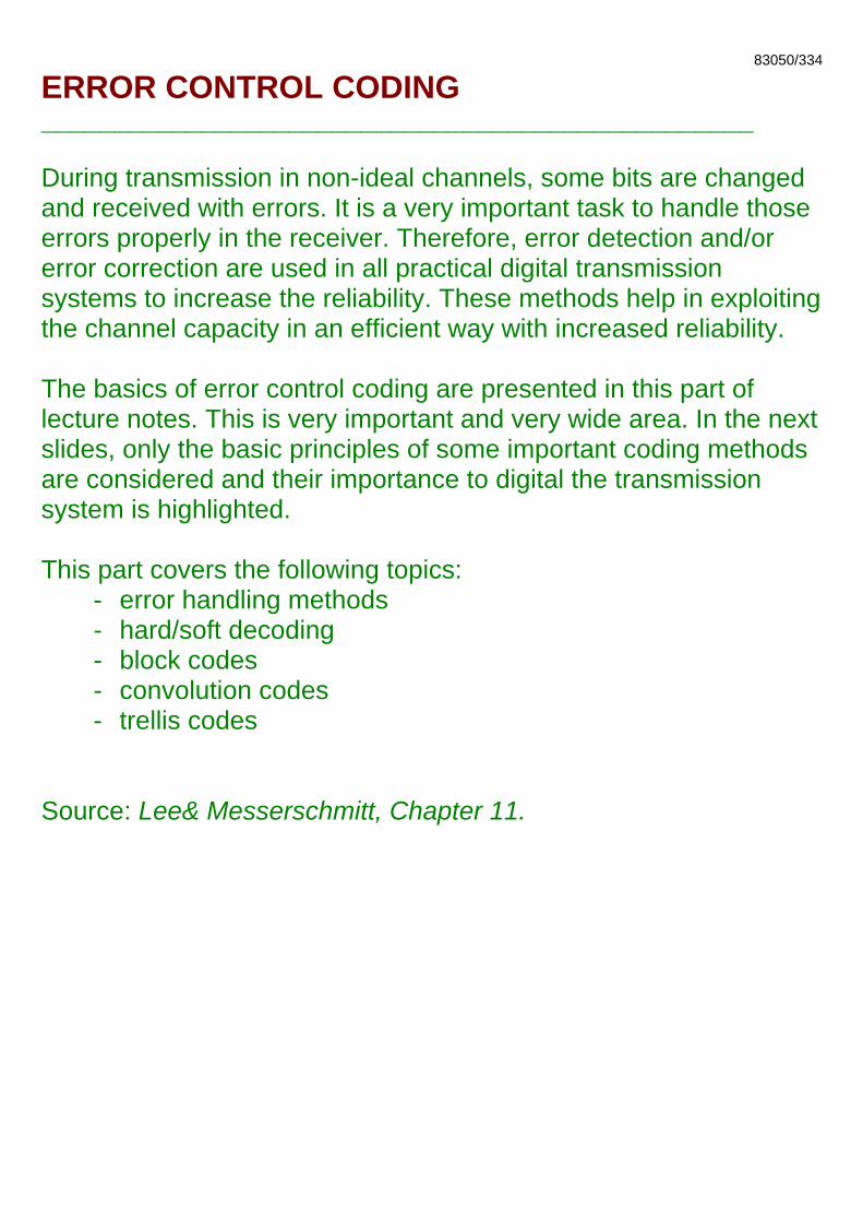
Cyclic Codes: Details (cont.) _________________________________________________

83050/361

Cyclic codes: Details (cont.) _________________________________________________

83050/362

Systematic Cyclic Codes _________________________________________________

83050/363

The Syndrome of Cyclic Codes _________________________________________________

83050/364

Example: Codes Used in GSM _________________________________________________

83050/365

Reed-Solomon Codes _________________________________________________ Reed-Solomon codes (RS codes) are defined for codeword lengths

12 −= mnwhere is a positive integer. Each codeword consists of mn symbols of m-bits. An ),( kn Reed-Solomon code is able to correct t=(n-k)/2 erroneous symbols in each codeword. It doesn’t make any difference whether a single bit or all the bits are wrong. Example: (255,235) -Reed-Solomon code is a commonly used basic code, e.g., in the family of DVB digital TV transmission systems. o codeword length is 255*8=2040 bits o each codeword carries 1880 information bits, consisting of

235 symbols of 8 bits. o the code is able to correct 10 erroneous symbols in each

codeword, i.e., maximally 80 erroneous bits (in case all the bits of all erroneous symbols are wrong)

o the code can correct any error burst of 72 consecutive bits within a codeword

83050/366

Shortened Reed-Solomon Codes _____________________________________________ In Reed-Solomon codes, the possible codeword lengths in bits are: 3x2, 7x3, 15x4, 31x5, 63x6, 127x7, 255x8, ... So there are only a rather limited sets of alternative lengths. More flexibility can be achieved by considering the so-called shortened Reed-Solomon codes (actually, the principle can be applied also for other block codes). Example: Using the basic (255,235) Reed-Solomon code, a shortened code (208, 188) can be derived as follows:

(1) In the coder, 235-symbol words are generated by inserting 47 0-symbols into the sequence of 188 symbols to be coded.

(2) These words are coded by using a coder for the basic (255, 235) RS code.

(3) The extra 47 zero symbols are removed from each codeword (their places are fixed and known in advance). The remaining 208 symbols are transmitted

(4) In the decoder, the zero symbols are again inserted to the proper positions, then the decoding is done using the decoder of the basic code, and the 188 information symbols are collected from the decoded sequence.

83050/367

Reed-Solomon Codes - Performance _________________________________________________

83050/368

7

CONVOLUTIONAL CODES _________________________________________________

A convolutional coder is a finite memory system, different from block coders which are memoryless. Convolutional codes are used more often than block codes, because they are conceptually and practically simpler, and their performance is better than the performance of good block codes. The performance is better mainly thanks to practical soft decoding techniques.

The main parameters: • Coding rate R=k/n. • Constraint length M (in some sources kM).

Convolutional codes are constructed using modulo two summations and delay elements.

The convolutional coder is working continuously: • Coder takes k input bits during each cycle. • It produces n output bits during each cycle. • Output bits are determined by using M previous source bits.

The code is systematic if all the k bits are passed to the output unchanged.

Convolutional codes can be described by using generator and parity check matrices, in the same way as block codes. In this case, these matrices have polynomials as entries, different from block codes where the entries were 0’s and 1’s.

It is also possible to represent the input bit sequence as polynomial in D (D is in place of z-1). This is a modulo-two z-transform representation:

Example: Bit sequence 1 0 0 1 1 0 0 1 has the "z-transform" 1 3 4+ + +D D D

83050/369

D

Generator Matrix and Parity Check Matrix _________________________________________________ The coder is defined by the following z-transform relation

C B G( ) ( ) ( )D D=

where G(D) is generator matrix and

[ ][ ])(,),(),()(

)(,),(),()()()2()1(

)()2()1(

DCDCDCD

DBDBDBDn

k

…

…

=

=

C

B

Here B and C are z-transforms of input and output bit sequences.

Di( ) ( ) )Di( ) (

The highest degree of G(D) is M−1, where M is constraint length of the code. If the code is systematic, the parity check and generator matrices are related, and they can be determined from each other. In the following examples, we can see how the generator and parity check matrices can be used in the same way as for block codes. We will also see an example of how non-systematic code can be modified to become systematic.

83050/370

Example I _________________________________________________ Code rate R=k/n=2/3 Constraint length M=2 Generator matrix:

⎥⎦⎤

⎢⎣

⎡ ⊕=

DD

D10

101)(G

The code is systematic. The parity check matrix is: H( ) , ,D D D= ⊕1 1

Let us now check if this is really a parity check matrix:

[ ]

0)()()1()()()1(

1

1)()()1(),(),()()(

)2()1()2()1(

)2()1()2()1(

=⊕⊕⊕⊕⊕=

⎥⎥⎥

⎦

⎤

⎢⎢⎢

⎣

⎡ ⊕⊕⊕=′

DDBDBDDDBDBD

DD

DDBDBDDBDBDD HC

This is valid for all codewords. The parity check matrix is very helpful for systematic codes. In this case it is possible to set C D , and

is determined using the parity check matrix: B D( ) ( )( ) ( ),1 1= C D B D( ) ( )( ) (2 2= )

)C D( ) (3

)()()1()(

0)()()()1()()()2()1()3(

)3()2()1(

DDCDCDDC

DCDDCDCDDD

⊕⊕=⇒

=⊕⊕⊕=′HC

83050/371

Example II _________________________________________________

Coder rate is R=k/n=1/2. Constraint length M=3. Generator matrix: G( ) ,D D D= ⊕ ⊕ ⊕1 12 2D

The code is not systematic.

Instead of parity check matrix, the following modulo two algebra can be used:

C D D B D

C D D D B D

( )

( )

( ) ( ) ( )

( ) ( ) ( )

1 2

2 2

1

1

= ⊕

= ⊕ ⊕ If both sides of the first equation are multiplied with ( ) and both sides of second equation with ( , then the left sides of these two equations are equal, and we can write

1 2⊕ ⊕D D)1 2⊕ D

( ) ( ) ( ) ( )( ) ( )1 12 1 2 2⊕ ⊕ = ⊕D D C D D C D or 0)()1()()1( )2(2)1(2 =⊕⊕⊕⊕ DCDDCDD Thus we can define a parity check matrix as

H( ) ( ), ( )D D D= ⊕ ⊕ ⊕1 12 2D .

83050/372

0

)

2

Example II (cont.) _________________________________________________ Given a parity check matrix, it is easy to design a systematic coder. First, we can write: C H( ) ( ) ( ) ( ) ( ) ( )( ) ( )D D D D C D D C D′ = ⊕ ⊕ ⊕ ⊕ =1 12 1 2 2

To get a systematic code, assign C D . Now we can write:

B D( ) ( ) (1 =

( ) ( ) ( ) ( )( )1 12 2⊕ ⊕ = ⊕D D B D D C D Based on this equation, it is possible to construct a systematic coder, as shown in figure (a). This system is a cascade of two linear subsystem whose order can be reversed to get the implementation in (b). (This is procedure used in design in recursive digital filters.)

This coder and the initial coder have the same parity check matrix. Further, in all important respects these two codes are equivalent.

83050/373

Decoding _________________________________________________ We consider here both hard decoding and soft decoding of convolutional codes. In general, soft decoding gives better performance.

In the case of convolutional codes, it is very natural to perform ML sequence detection. The decoder chooses the sequence that is closest to the observation in Hamming or Euclidean distance.

It is convenient to represent convolutional codes as Markov chains, as convolutional coding is a shift register process.

The state transition diagram of a code can be represented by using the trellis diagram. The trellis diagram shows the progression through states over time. The state of the code (Markov chain) corresponds to the bits stored in the delay elements in the coder.

The decoder complexity depends essentially on the number of states in the diagram, which is determined by the total number of shift-register stages in the coder. The number of states is less than or equal to 2k(M-1).

The decoder chooses the shortest path based on the received sequence. Example I: Below one stage of the trellis diagram of the example code with R=2/3 is shown. The number of states is 4 and the trellis is fully connected.

83050/374

Example II _________________________________________________ In this case there are two bits in the delay line of the coder. The number of states is 4. Below different versions of the trellis diagram are shown.

83050/375

About the Performance of Decoders _________________________________________________

This is a coded transmission system with a soft decoder. We assume additive white Gaussian noise and binary antipodal signalling, in which case Viterbi algorithm can be used for performing optimal ML-sequence detection. These are the important parameters for coded and uncoded signalling: uncoded coded channel symbols ±au ac

σu2 σc

2

[ ] [ ]

± noise variance In the following, we compare the performance of uncoded and coded systems, based on soft and hard decoding. The analysis is done for the convolutional code with rate ½, that was introduced earlier. For uncoded system, the probability of symbol error is equal to probability of bit error:

⎟⎟⎠

⎞⎜⎜⎝

⎛==

u

uaQerrorsymbolerrorbit

σ Pr Pr

83050/376

Example I: Soft Decoding _________________________________________________ In the following we use the notation: - Noisy observations: y yk k, ,+1 …

- Detected symbols: a a, ,k k+1 …

( )

One stage of the trellis diagram with all possible transitions is given here. It is used for decoding of one single bit. The ML detector computes the branch metrics as

( )21122 ˆˆ ++ −+−= kkkk ayayd

The ML- decoder chooses the path with minimum path metrics. For soft decoding, the Euclidean metric is used. Probability of error depends on the error event with minimum distance. For this example case, the minimum distance error path (critical path) is shown in the following figure.

The square of the Euclidean distance between the correct path and the error event is: d acmin

2 220=In this case, it is easy to check that there are no distinct paths that are closer to each other. Furthermore, due to the linearity of the code, there are similar error events in every possible correct path.

83050/377

[ ]

Example I: Soft Decoding (cont.) _________________________________________________ The probability of symbol error can be expressed as:

⎟⎠⎞

⎜⎝⎛=

σ2mindKQ

[ ] [

Pr errorsymbol

In the example case, the symbol error is same as bit error, thus:

] ⎟⎟⎠

⎞⎜⎜⎝

⎛=⎟⎟

⎠

⎞⎜⎜⎝

⎛

cc

cc aQaQ

σσ5

220

== errorsymbolerrorbit PrPr

Here dmin is minimum Euclidean distance of an error event, and K is a constant. In general, finding K and dmin can be very difficult. If the code is linear, this is simplified by using Viterbi algorithm in a modified form. If the transmission rate is same, in coded system the signal bandwidth is doubled. This means that the noise power in coded system is twice the noise power of uncoded system, i.e.

σ σc u= 2

uc SNRSNR =5

If it is desired to achieve the same performance with coded and uncoded systems, then the argument of Q function should be the same, in other words

If we take into account increased noise level in the coded system then:

a a au

u

c

c uσ σ= =

dB 4)2/5(log10 10

cσ

5 52

So the true coding gain is =

83050/378

Performance of Hard Decoding: Example I _________________________________________________ In the following, the hard decoding is compared to both soft decoding and uncoded system. For hard decoder, the channel can be modelled as a BSC. The analysis is similar to analysis for soft decoding. The main differences are: • The Hamming distance is used • Instead of error function Q(), the binomial Q( , )-function is

used to calculate probability of error. A critical error path is given below:

Here, the correct bit sequence is: (0,0) (0,0) (0,0) The error sequence is : (1,1) (0,1) (1,1) The corresponding Hamming distance is 5, and the probability of error becomes:

Pr Pr

( , ) ( ) ( )

bit error

Q p p p p p p= = − + − +

detectio= n error

5 10 1 5 13 2 4 5

For small value of error probability in BSC, this is approximated by:

Pr bit error p= 10 3

83050/379

10 10 0 013 5p p= ⇒ =− .

Performance of Hard Decoding: Example I (cont.) _________________________________________________ For comparison, we assume the same probability of error for coded and uncoded systems, e.g., 10-5. Then it is possible to derive p for the BSC model of coded system: The signalling is antipodal, therefore:

Q a Q a ah c h u h u( / ) ( / ) . .σ σ σ= = ⇒ =2 0 01 3 4

u u= 4 3.

In the uncoded system, the same probability of error is achieved when a σ : Thus the coding gain becomes: 20 4 3 3 410log ( . / . ) 2≈ dB This is smaller compared to case of soft decoding (it was 4 dB)

83050/380

More about Convolutional Codes _________________________________________________ The concept of free distance, dfree, has the same significance for convolutional codes as Hamming distance has in case of block codes. It gives an idea about the performance of the code. As an example, for the code of page 371, the free distance is 5. Good convolutional codes have been found through computer search methods. The following table gives some of those. The elements of the generator matrix are given there in octal form. As an example, the first code of the table is one of the widely used examples in the Lee&Messerschmitt book (se page 371).

83050/381

Punctured Convolution Codes ___________________________________________________ Puncturing means that some of the bits from the output of a normal convolutional coder are removed, in a regular pattern. This is done, of course, in such way that the data can be perfectly decoded in case of ideal channel. In puncturing, the code-rate is increased, but the free distance is reduced. The following table lists some punctured codes for rates 2/3 and 3/4. In both cases, the basic code is the rate 1/2 convolution code of page 371.

83050/382

,...,,,,,,,, )1(7

)2(6

)1(5

)2(4

)1(4

)2(3

)1(2

)2(1

)1(1 CCCCCCCCC

Punctured Convolution Codes (cont.) ___________________________________________________ Example: The code with transfer matrix (7,5,7,x) is obtained from the basic code of page 371 (see below) by forgetting every other C1

k ouput. The code with transfer matrix (5,7,5,x,x,7) is obtained from the basic code of page 371 (see below) by sending the following bit-stream:

One very interesting feature of puncturing is that several codes with different rates can be obtained form a single basic code. This makes it possible to develop systems, where the useful bit-rate and error correction performance can be traded-off in a flexible way. Such approach is used in the new European digital TV systems, DVB-T and DVB-S.

83050/383

Comparisons of Convolution Codes I _____________________________________________

83050/384

Comparisons of Convolution Codes II

83050/385

Concatenated Coding ____________________________________________ A commonly used solution in digital transmission systems (e.g., DVB systems) includes two different error correcting codes, and also interleaving in between:

This has turned out to be a practical way to design error control coding systems that provide a very low BER for the application, using a rather low SNR (or high ‘raw BER’ before the channel decoder). Typically, the ‘raw BER’ is 0.1…0.01, the BER after convolution decoding 10-3…10-4, and the BER after block decoder 10-9…10-12. On the other hand, such solutions with rather high ‘raw BER’ make it possible to get closer to channel capacity than using higher SNR.

83050/386

Concatenated Coding (cont.) ____________________________________________ The inner code is typically a convolution code (or trellis code or, in latest developments, a turbo code, an advanced structure based also on convolutional coding ideas). Using convolution type of code makes it possible to get the benefit of soft decoding, which is very important when the ‘raw BER’ is high. Using the puncturing ideas, it is also possible to make flexible system, where the code rate and the SNR requirements can be adapted according to the channel conditions and application requirements. The outer code is typically a block code, like Reed-Solomon. The channel and the inner decoder produce often error bursts, and by using the (de)interleaver, the burst errors are spread out evenly in the symbol stream going to the outer coder. This helps the outer decoder in its tasks and thus helps to reduce the final bit error rate.

83050/387

Interleaving ___________________________________________ In interleaving, the symbol/bit stream is reordered deterministically. The goal is to move the consecutive bits coming from the channel as far as possible from each others. This removes the correlations in the bit/symbol-stream.

The lengths of the interleavers to be used in practice are limited by o required memory needed for the interleaver o induced processing delay.

Interleaving is commonly used in the context of concatenated coding, but it can also be used otherwise to reduce the correlations in the bit/symbol streams.

There are two commonly used principles for interleaving: - Block interleaving: The incoming symbol stream is written into

an MxN table column-wise and read out row-wise. The de-interleaver is, of course, implemented in the opposite way.

- Convolution interleaving: This is a slightly more complicated structure, saving about half of the needed memory:

83050/388

TRELLIS CODING _____________________________________________ In the case of block and convolutional codes, the redundancy was introduced by adding some symbols in the symbol stream. Thus, the symbol rate and required bandwidth are increased. This will increase the noise in the system. Therefore, the designed code must have larger coding gain to compensate this. It is possible to introduce the redundancy by using larger constellation, i.e., by using more symbols in the alphabet. In this case the symbol rate is not changed. This technique is useful for band limited signals. The resulting code is sometimes called signal-space code. The symbols in the new constellation are more closely spaced, and the noise immunity is reduced. The coding gain must be high enough to compensate for this. The input constellation size is 2k, with k bits per symbol, and after coding the size of constellation is 2n. Thus a code with code rate k/n is needed.

The code to introduce redundancy can be a block code or a convolutional code. When a convolutional code is used to get a signal-space code, the result is called a trellis code. Source: Lee&Messerschmit, Chapter 12.

83050/389

Coded Modulation _____________________________________________ Assume that we have an AWGN channel, and an acceptable data rate is achieved with constellation size of M and probability of error is achieved without coding at some SNR. Using coding it is possible to: • Reduce the error probability by keeping the same SNR, or • Achieve the same error probability with smaller SNR.

The improvements in performance are limited by the Shannon channel capacity (see pages 26 and 27). Below, we show the key observation that the most of this theoretical maximum improvement can be achieved using a constellation of size 2M and suitable code. Example: It is desired to have rate of 4 bits per symbol and probability of error not larger than 10-5. • 16-QAM case: required SNR is 19 dB • 32-QAM, theoretical lower bound for SNR is 13 dB

o obtained coding gain is 6dB • Shannon bound is 11.7 dB

o With larger constellations, the coding gain could be improved by 1.3 dB, at most.

The coding gain of 3-4 dB can usually be achieced easily. Trellis coding is commonly used in various applications, like voice band modems.

83050/390

About the Performance of Trellis Codes _____________________________________________ The performance of trellis codes depends on the number of states in trellis diagram of the used code. The following table gives some idea about the achievable performance. Number coding

of states gain ----------------------------- 4 3 dB 8 4 dB 16 close to 5 dB 128 close to 6 dB By their nature, trellis codes lend themselves to soft decoding using the Viterbi algorithm. At reasonably high SNR, the symbol error probability is given by: Pr /,minsymbol error KQ dE= 2σ

Here K is a constant (between lower and upper limits given in the book by Eqs. (7.95) and (7.87)). In simple example cases, the value of K can be determined easily. However, in many cases the constant is approximated K=1. The performance of trellis codes is dominated by the error event with minimum Euclidean distance. In general, trellis codes are not linear even when the underlying convolutional code is linear. In this case it is not safe to simplify the calculation of minimum distance by finding the error event closest to the zero state trajectory. Instead, one has to find systematically the minimum distance error event for each possible correct path through the trellis, e.g., using a modification of the Viterbi-algorithm.

83050/391

Example of Basic Trellis Codes _____________________________________________ In the following, a simple trellis code is presented. It uses convolutional code with rate R=1/2, 4-PSK modulation and 1 bit per symbol. The convolutional coder (without the line coder) has been considered earlier in this material.

83050/392

Performance of Basic Trellis Codes _____________________________________________ In the previous slide, we have seen the minimum distance error event assuming the correct state trajectory is zero. The distance is calculated using complex arithmetic:

d a a a ja a a aE,min = + + − + + =2 2 2 10 It is easy to observe that this is error event with minimum distance, based on the following facts:

- all branches diverging from the same node have distance 2a from each other

- all branches converging on the same node have distance 2a - after two parts diverge, all possible combinations of subsequent

branches have distance : 2a Thus, the minim distance is:

d a a a aE,min ( ) ( )≥ + + =2 2 2 102 2 2

[ ] [ ]

The probability of error is obtained as:

⎥⎦

⎤⎢⎣

⎡≈≈

σ210PrPr aQerrorsymbolerrorbit

[ ]

In the example case, every state trajectory, corresponding to 3 symbols, has exactly one error event at minimum distance, and this error event has exactly one symbol error, so K=1. To compare this performance to an uncoded system, we first observe that the noise variance is the same in both cases because the signal bandwidth is the same. An uncoded 2-PSK system has the same transmit power as coded 4-PSK, and carries the same number of source bits. The probability of error is:

⎥⎦⎤

⎢⎣⎡=σaQerrorbitPr

Thus the coding gain is: 20 10 2 4log( / ) = dB The same improvement is achieved by convolutional coding with soft decoding, but in the case of trellis coding without increasing the bandwidth. Trellis coding is usually preferred over convolutional or block coding for bandlimited channels, unless nonlinearities or hardware complexity make them impractical.

83050/393

More Elaborate Trellis Codes _____________________________________________ In the above example, one source bit was processed to give two coded output bits. Two coded bits are used to produce alphabet of size four. The technique can be easy extended to make use of alphabet larger than four.

In this figure, the trellis code is extended by using one uncoded bit and a larger alphabet (size 8 in this case), thus the number of source bits per symbol is increased. The transition from one state to another is controlled entirely by the source bit that goes to the coder. Each transition from one state to another occurs for two possible values of uncoded source bit, zero and one. This can be represented by showing two parallel transitions between every pair of states in trellis diagram. The trellis diagram of the figure below corresponds to example of the figure above.

83050/394

More Elaborate Trellis Codes (cont.) _____________________________________________ This technique can be generalized as shown here. First, based on bandwidth limitations, determine the symbol rate that can be transmitted. Next, determine the size of alphabet 2m that would be required (without coding) to transmit the source bits at the desired rate. Then double the size of alphabet to 2m+1 and introduce a channel coder that produces the extra bit. The coder does not need to code all incoming bits, however leaving some bits uncoded can affect performance.

This figure shows a general trellis coder. The incoming source bits are divided into bits to be coded and m̂ m̂m − bits to be left uncoded. The required convolutional coder has rate )1ˆ/(ˆ +mm

mm ˆ2 −, and

the trellis will have parallel transitions between every pair of states.

83050/395

Bit Mapping for Trellis Codes _____________________________________________ To complete the coder design, we need to design the mapping of bits into symbols. Designing the mapping is the same as assigning symbols to transitions in the trellis diagram. When there are parallel transitions, a very short error event consist of mistaking one of these parallel transitions for the correct one. To minimize error probability, we should ensure that the Euclidean distance between the symbols corresponding to parallel transitions is maximized. For example with 8-PSK, this can done as illustrated in the following. The constellation is divided into four subsets. To ensure that parallel transitions in trellis have symbols as far apart as possible, symbols for parallel transitions are selected form the same subset. Now, assign subsets to pairs of transitions to try to maximize the minimum distance. This can be done by keeping the distance between diverging or merging branches as large as possible.

The performance of the code is dominated by the error event with the smallest distance from the correct path

83050/396

Bit Mapping for Trellis Codes, Example _____________________________________________ Using mapping for 8-PSK explained above, the distance between parallel transitions is 2a (a is the amplitude of 8-PSK), and this is the minimum distance. The probability of error event is given as:

⎟⎠⎞

⎜⎝⎛=σaQeventerror ) Pr(

The error events result in exactly one bit error out of two uncoded bits, and there is only one such event for each correct path, thus:

⎟⎠⎞

⎜⎝⎛≈σaQerrorbit

21) Pr(

This can be compared to the uncoded system, which corresponds to 4-PSK:

⎟⎟⎠

⎞⎜⎜⎝

⎛=

σaQerrorbit 2) Pr(

dB32log20 =Ignoring the constant multiplier, the coding gain is: ,

and this is 1dB lower compared to the system without parallel transitions.

83050/397

Mapping by Set Partitioning _____________________________________________ A systematic way to design bit mappings in such way that the parallel transitions correspond to symbols that are as far apart as possible is generally known as mapping by set partitioning. Once the alphabet is chosen and the number of coded and uncoded bits selected, we still have freedom to map the coded bits into symbols. The choice of mapping can affect the performance of the code. Example 1: Systematic partitioning of an 8-PSK constellation

Example 2: Systematic partitioning of an 16-QAM constellation

Note that the uncoded bits select a signal from subset, and the coded bits select the subset. The general rules for mapping by set partitioning are: • maximize the distance between parallel transitions first • maximize the distance between transitions originating or

ending in the same state • use all symbols with equal probability.

83050/398

Mapping by Set Partitioning: Example _____________________________________________ A trellis coder with one uncoded bit and two coded bits with 16-QAM from previous slide. The convolutional coder is an 8 state, rate 2/3, and of feedback type.

The corresponding trellis diagram:

The coding gain of this coder is about 5.33 dB. If one more uncoded bit is used with 32-QAM ,the coding gain reduces to 3.98 dB, with two more uncoded bits (64-QAM) the coding gain reduces to 3.77 dB.

83050/399

Catastrophic Codes _____________________________________________ In most cases we have assumed that there is only one minimum distance error event, and it dominates the performance. The code that has unbounded number of minimum distance error events is called catastrophic. Example: A four point constellation with partition shown below. We consider transmitting 2 bits per symbol. This can be represented by using two state trellis. We can see that there is infinite number of error events with same (finite) minimum distance. In this case, we should not expect any coding gain at all, because we are representing two source bits with an alphabet of size four (no redundancy).

Catastrophic codes have property that there are error events with finite distance but infinite length.

83050/400

Multidimensional Trellis Codes _____________________________________________

Some of the most interesting trellis codes in use are multidimensional trellis codes. The idea of these codes is to overcome one of the main limitations of trellis codes, the requirement that the size of the symbol alphabet be doubled. (Recall the observation that doubling the symbol alphabet is sufficient to achieve almost all available coding gain). However, doubling the alphabet for the same average power reduces the spacing between symbols and reduces noise margin by about 3 dB. In case of a multidimensional trellis code, doubling the alphabet entails less than 3 dB loss in noise margin. Example: We consider a four dimensional symbol

[ ] { }1,3 where,4,,, 321 ±±∈= ik aaaaaA There are 256 symbols in this alphabet, with average power 20. A four dimensional alphabet with 512 symbols and average power 27 is constructed by adding symbols of the form { }1,1,3,5 ±±±± , and all it permutations, and symbols of form { }1,1,1,5 ±±±± and all its permutations. Given a two dimensional modulation system the first two coefficients of the four dimensional system are transmitted in one symbol interval as the real and imaginary part of a complex symbol, and the last two in the next symbol interval.

The trellis coder that makes use of this is shown here. The four dimensional alphabet has 512 symbols, and can represent 9 bits. Three bits are coded to get four bits, and five bits are used uncoded. The coding gain of this structure is about 4.7dB. The two dimensional trellis coder with same source bit rate has coding gain of 4dB.

83050/401

)1(kC )2(

kC

)3(kC )4(

k

Trellis Codes using Non-Linear Convolutional Codes _____________________________________________ Some desirable properties can be obtained by using non-linear convolutional codes. One example coder is the following, which is adopted in the ITU-T recommendation V.32 for voiceband modem. The main advantage of this code is that it is invariant over 90 degree phase shifts, which is a big advantage in the context of carrier recovery. Some of symmetry is evident from constellation. It is evident that and are the same at all points 90 degrees apart. Furthermore, and C differentially encode the quadrant, i.e., to move for -90 degrees, simply add one to these two bits. This differential encoding is introduced by the differential encoder in the figure.