Embed Size (px)
Citation preview

Proximal-Proximal-Gradient Method
Ernest K. Ryu and Wotao Yin
October 19, 2017
Abstract
In this paper, we present the proximal-proximal-gradient method (PPG),a novel optimization method that is simple to implement and simple toparallelize. PPG generalizes the proximal-gradient method and ADMMand is applicable to minimization problems written as a sum of manydifferentiable and many non-differentiable convex functions. The non-differentiable functions can be coupled. We furthermore present a relatedstochastic variation, which we call stochastic PPG (S-PPG). S-PPG canbe interpreted as a generalization of Finito and MISO over to the sum ofmany coupled non-differentiable convex functions.
We present many applications that can benefit from PPG and S-PPGand prove convergence for both methods. We demonstrate the empiricaleffectiveness of both methods through experiments on a CUDA GPU. Akey strength of PPG and S-PPG is, compared to existing methods, theirability to directly handle a large sum of non-differentiable non-separablefunctions with a constant stepsize independent of the number of functions.Such non-diminishing stepsizes allows them to be fast.
1 Introduction
In the past decade, first-order methods like the proximal-gradient method andADMM have enjoyed wide popularity due to their broad applicability, simplicity,and good empirical performance on problems with large data sizes. However,there are many optimization problems such existing simple first-order meth-ods cannot directly handle. Without a simple and scalable method to solvethem such optimization problems have been excluded from machine learning andstatistical modeling. In this paper we present the proximal-proximal-gradientmethod (PPG), a novel method that expands the class of problems that onecan solve with a simple and scalable first-order method.
Consider the optimization problem
minimize r(x) +1
n
n∑i=1
(fi(x) + gi(x)), (1)
where x ∈ Rd is the optimization variable, f1, . . . , fn, g1, . . . , gn, and r areconvex, closed, and proper functions from Rd to R∪∞. Furthermore, assume
1
arX
iv:1
708.
0690
8v2
[m
ath.
OC
] 1
8 O
ct 2
017

f1, . . . , fn are differentiable. We call the method
xk+1/2 = proxαr
(1
n
n∑i=1
zki
)xk+1i = proxαgi
(2xk+1/2 − zki − α∇fi(xk+1/2)
)zk+1i = zki + xk+1
i − xk+1/2, (PPG)
the proximal-proximal-gradient method (PPG). The xk+1i and zk+1
i updates areperformed for all i = 1, . . . , n and α > 0 is a stepsize parameter. To clarify,x, x1, . . . , xn and z1, . . . , zn are all vectors in Rd (xi is not a component of x),xk+1
1 , . . . , xk+1n and xk+1/2 approximates the solution to Problem (1).
Throughout this paper we write proxh for the proximal operator with respectto the function h, defined as
proxh(x0) = argminx
h(x) +
1
2‖x− x0‖22
for a function h : Rd → R ∪ ∞. When h is the zero function, proxh isthe identity operator. When h is convex, closed, and proper, the minimizerthat defines proxh exists and is unique [39]. For many interesting functions h,the proximal operator proxh has a closed or semi-closed form solution and iscomputationally easy to evaluate [11, 44]. We loosely say such functions areproximable.
In general, the proximal-gradient method or ADMM cannot directly solveoptimization problems expressed in the form of (1). When f1, . . . , fn are notproximable, ADMM either doesn’t apply or must run another optimization al-gorithm to evaluate the proximal operators at each iteration. When n ≥ 2 andg1, . . . , gn are nondifferentiable nonseparable, so g1 + · · ·+ gn is not proximable(although each individual g1, . . . , gn is proximable). Hence, proximal-gradientdoesn’t apply.
One possible approach to solving (1) is to smooth the non-smooth parts andapplying a (stochastic) gradient method. Sometimes, however, keeping non-smooth part is essential. For example, it is the non-smoothness of total variationpenalty that induces sharp edges in image processing. In these situations (PPG)is particularly useful as it can handle a large sum of smooth and non-smoothterms directly without smoothing.
Distributed PPG. To understand the algorithmic structure of the method, itis helpful to see how (PPG) is well-suited for a distributed computing network.See Figure 1, which illustrates a parameter server computing model with amaster node and n worker nodes.
At each iteration, the workers send their zki to the parameter server, theparameter server computes xk+1/2 and broadcasts it to the workers, and eachworker i computes zk+1
i with access to fi, gi and zki for i = 1, . . . , n. The workersmaintain their private copy of zki and do not directly communicate with eachother.
2

Parameter server
Worker 1 (zk1 ) Worker 2 (zk2 ) · · · Worker n (zkn)
Figure 1: When (PPG) is implemented on a parameter server computing model,the worker nodes communicate (synchronously) with the parameter server butnot directly with each other.
In other words, a distributed implementation performs step 1 of (PPG), thexk+1/2 update, with an all-reduce operation. It performs step 2 and step 3, thexk+1i and zk+1
i updates, in parallel.
Time complexity, space complexity, and parallelization. At each itera-tion, (PPG) evaluates the proximal operators with respect to r and g1, . . . , gnand computes the gradients of f1, . . . , fn. So based on the iteration cost alone,we can predict (PPG) to be useful when r and g1, . . . , gn are individually prox-imable and the gradients of f1, . . . , fn are easy to evaluate. If, furthermore,the number of iterations required to reach necessary accuracy is not exorbitant,(PPG) is actually useful.
Let’s say the computational costs of evaluating proxαr is cr, proxαgi is cgfor i = 1, . . . , n, and ∇fi is cf for i = 1, . . . , n. Then the time complexity of(PPG) is O(nd+cr+ncg+ncf ) per iteration (recall x ∈ Rd). As discussed, thiscost can be reduced with parallelization. Computing xk+1/2 involves computingan average (a reduce operation), computing proxαr, and a broadcast, and com-puting zk+1
i for i = 1, . . . , n is embarrassingly parallel. The space complexity of(PPG) is O(nd) since it must store zk1 , . . . z
kn. (xk1 , . . . , x
kn need not be stored.)
When the problem has sparse structure, the computation time and storagecan be further reduced. For example, if fi + gi does not depend on (xi)1 forsome i, then (zi)1 and (xi)1 can be eliminated from the algorithm since (zi)
k+11 =
(xk+1/2)1.The storage requirement of O(nd) is fundamentally difficult to improve upon
due to the n non-differentiable terms. Consider the case where r = f1 = · · · =fn = 0:
minimize g1(x) + · · ·+ gn(x).
If g1, . . . , gn were differentiable, then ∇g1(x∗) + · · ·+∇gn(x∗) = 0 would certifyx∗ is optimal. However, we allow g1, . . . , gn to be non-differentiable, so onemust find a particular set of subgradients ui ∈ ∂gi(x
∗) for i = 1, . . . , n suchthat u1 + · · · + un = 0 to certify x∗ is optimal. The choices of subgradients,u1, . . . , un, depend on each other and cannot be found independently. In otherwords, certifying optimality requires O(nd) information, and that is what PPGuses. For comparison, ADMM also uses O(nd) storage when used to minimize
3

a sum of n non-smooth functions.
Stochastic PPG. Each iteration of (PPG) updates zk+1i for all i = 1, . . . , n,
which takes at least O(nd) time per iteration. In Section 3 we present themethod (S-PPG) which can be considered a stochastic variation of (PPG). Eachiteration of (S-PPG) only updates one zk+1
i for some i and therefore can takeas little as O(d) time per iteration. When compared epoch by epoch, (S-PPG)can be faster than (PPG).
Convergence. Assume Problem (1) has a solution (not necessarily unique)and meets a certain regularity condition. Furthermore, assume each fi in hasL-Lipschitz gradient for i = 1, . . . , n, so ‖∇fi(x)−∇fi(y)‖2 ≤ L‖x− y‖2 for allx, y ∈ Rd and i = 1, . . . , n. Then (PPG) converges to a solution of Problem (1)for 0 < α < 3/(2L). In particular, we do not need strong convexity to establishconvegence.
In section 4 we discuss convergence in more detail. In particular, we proveboth that the iterates converge to a solution and that the objective values con-verge to the optimal value.
Contribution of this work. The methods of this paper, (PPG) and (S-PPG),are novel methods that can directly handle a sum of many differentiable and non-differentiable but proximable functions. To solve such problems, exising first-order methods like ADMM must evaluate proximal operators of differentiablefunctions, which may hinder computational performance if said operator has noclosed form solution. Furthermore, the simplicity of our methods allows simpleand efficient parallelization, a point we discuss briefly.
The theoretical analysis of (PPG) and (S-PPG), especially that of (S-PPG),is novel. As we discuss later, (S-PPG) can be interpreted as a generalization tovarianced reduced gradient methods like Finito/MISO or SAGA. The techniqueswe use to analyze (S-PPG) is different from those used to analyze other vari-anced reduced gradient methods, and we show more general (albeit not faster)convergence guarantees. In particular, we establish almost sure convergence ofiterates, and we do so without any strong convexity assumptions. To the best ofour knowledge, the existing varianced reduced gradient method literature doesnot prove such results.
Finally, our method is the first work to establish a clear connection betweenoperator splitting methods and varianced reduced gradient methods. As thename implies, existing varianced reduced gradient methods view the method asimproving, by reducing variance, stochastic gradient methdos. Our work identi-fies Finito/MISO as stochastic block-coordinate update applied to an operatorsplitting method. It is this observation that allows us to analyze (S-PPG), whichgeneralizes Finito/MISO to handle a sum of non-differentiable but proximablefunctions.
4

2 Relationship to other methods
In this section, we discuss how (PPG) generalizes certain known methods. Toclarify, PPG is a proper generalization of these existing methods and cannot beanalyzed as a special case of one of these methods.
Proximal-gradient. When gi = 0 for i = 1, . . . , n in (1), (PPG) simplifies to
xk+1 = proxαr
(xk − α
n
n∑i=1
∇fi(xk)
).
This method is the called proximal-gradient method or forward-backward split-ting [45, 13].
ADMM. When f = r = 0 in (1), (PPG) simplifies to
xk+1i = argmin
x
gi(x)− (yki )Tx+
1
2α‖x− xk‖22
yk+1i = yki + α(xk+1 − xk+1
i )
where
xk+1 =1
n
n∑i=1
xk+1i .
This is also an instance of ADMM [21, 20]. See §7.1 of [8].
Generalized forward-backward splitting. When r = 0 and f1 = f2 = · · · =fn = f in (1), (PPG) simplifies to
zk+1i = zki − xk + proxαgi
(2xk − zki − α∇f(xk)
)xk+1 =
1
n
n∑i=1
zk+1i .
This is an instance of generalized forward-backward splitting [46].
Davis-Yin splitting. When n = 1 in (1), (PPG) reduces to Davis-Yin split-ting, and much of convergence analysis for (PPG) is inspired by that of Davis-Yin splitting [15]. However, (PPG) is more general and parallelizable. Further-more, (1) has a stochastic variation (S-PPG).
3 Stochastic PPG
Each iteration of (PPG) updates zk+1i for all i = 1, . . . , n, which requires at
least O(nd) time (without parallelization or sparse structure). Often, the datathat specifies Problem (1) is of size O(nd), and, roughly speaking, (PPG) mustprocess the entire dataset every iteration. This cost of O(nd) time per iterationmay be inefficient in certain applications.
5

The following method, which we call the stochastic proximal-proximal-gradientmethod (S-PPG), overcomes this issue:
xk+1/2 = proxαr
(1
n
n∑i=1
zki
)i(k) ∼ Uniform(1, . . . , n)
xk+1i(k) = proxαgi(k)
(2xk+1/2 − zki(k) − α∇fi(k)(x
k+1/2))
zk+1j =
zki(k) + xk+1
i(k) − xk+1/2 for j = i(k),
zkj for j 6= i(k).(S-PPG)
At each iteration, only zk+1i(k) is updated, where the index i(k) is chosen uni-
formly at random from 1, . . . , n. We can interpret (S-PPG) as a stochastic orcoordinate update version of (PPG).
Time and space complexity. The space requirement of (S-PPG) is no dif-ferent from that of (PPG); both methods use O(nd) space to store zk1 , . . . , z
kn.
However, the cost per iteration of (S-PPG) can be as low as O(d). This isachieved with the following simple trick: maintain the quantity
zk =1
n
n∑i=1
zki ,
and update it with
zk+1 = zk + (1/n)(xk+1i(k) − x
k+1/2).
Application to big-data problems. Consider a big-data problem setupwhere the data that describes Problem (1) is stored on a hard drive, but istoo large to fit in a system’s memory. Under this setup, an optimization algo-rithm that goes through the entire dataset every iteration is likely impractical.
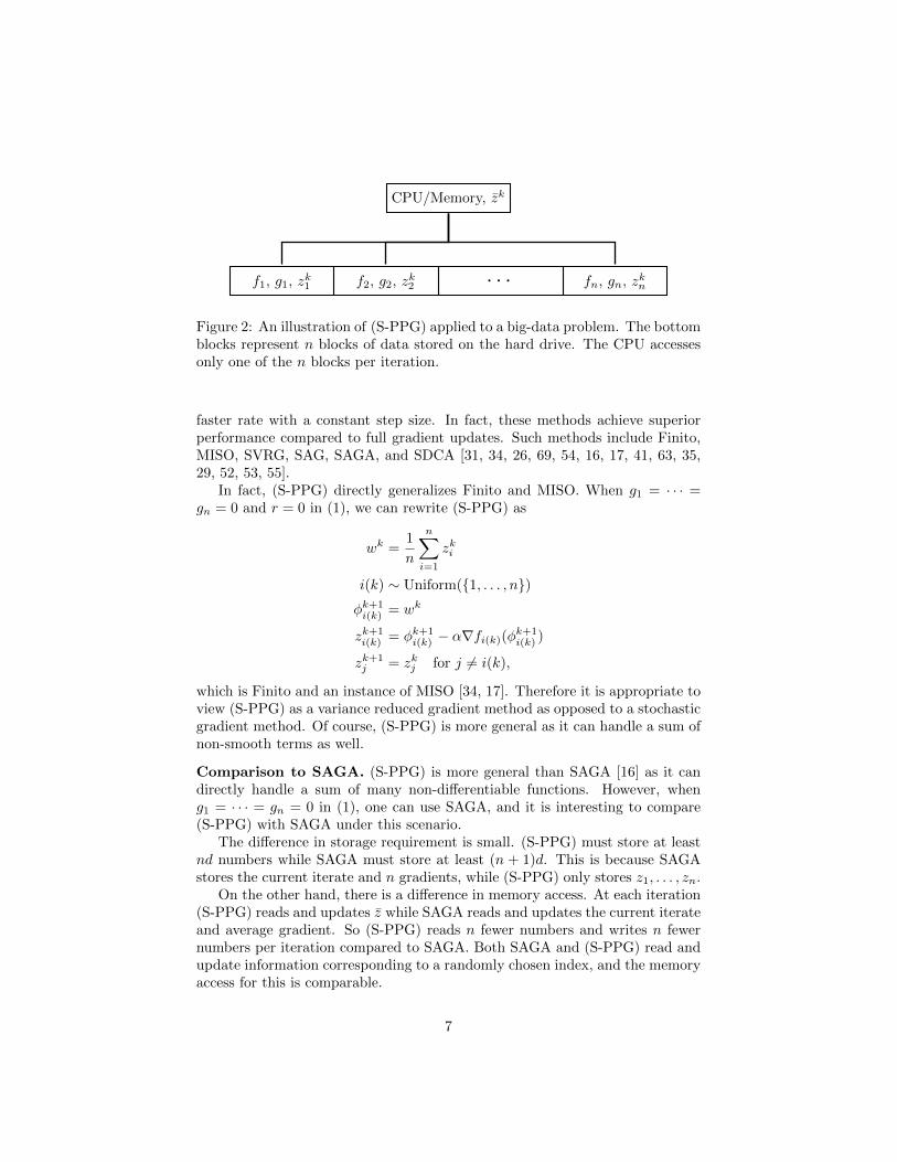
(S-PPG) can handle this setup effectively by keeping the data and the zkiiterates on the hard drive as illustrated in Figure 3. At iteration k, (S-PPG)selects index i(k), reads block i(k) containing fi(k), gi(k), and zki(k) from the
hard drive, performs computation, updates zk+1, and writes zk+1i(k) back to block
i(k). The zk iterate is used and updated every iteration and therefore shouldbe stored in memory.
Interpretation as a variance reduced gradient method. Remarkably(S-PPG) converges to a solution with a fixed value of α (which is independentof n). Many traditional and modern stochastic optimization methods requiretheir step sizes to diminish to 0, theoretically and empirically, and this limitstheir rates of convergence.
On the other hand, several modern “variance reduced gradient” methodstake advantage of a finite sum structure similar to that of (1) and achieve a
6
CPU/Memory, zk
f1, g1, zk1 f2, g2, zk2 · · · fn, gn, zkn
Figure 2: An illustration of (S-PPG) applied to a big-data problem. The bottomblocks represent n blocks of data stored on the hard drive. The CPU accessesonly one of the n blocks per iteration.
faster rate with a constant step size. In fact, these methods achieve superiorperformance compared to full gradient updates. Such methods include Finito,MISO, SVRG, SAG, SAGA, and SDCA [31, 34, 26, 69, 54, 16, 17, 41, 63, 35,29, 52, 53, 55].
In fact, (S-PPG) directly generalizes Finito and MISO. When g1 = · · · =gn = 0 and r = 0 in (1), we can rewrite (S-PPG) as
wk =1
n
n∑i=1
zki
i(k) ∼ Uniform(1, . . . , n)φk+1i(k) = wk
zk+1i(k) = φk+1
i(k) − α∇fi(k)(φk+1i(k) )
zk+1j = zkj for j 6= i(k),
which is Finito and an instance of MISO [34, 17]. Therefore it is appropriate toview (S-PPG) as a variance reduced gradient method as opposed to a stochasticgradient method. Of course, (S-PPG) is more general as it can handle a sum ofnon-smooth terms as well.
Comparison to SAGA. (S-PPG) is more general than SAGA [16] as it candirectly handle a sum of many non-differentiable functions. However, wheng1 = · · · = gn = 0 in (1), one can use SAGA, and it is interesting to compare(S-PPG) with SAGA under this scenario.
The difference in storage requirement is small. (S-PPG) must store at leastnd numbers while SAGA must store at least (n + 1)d. This is because SAGAstores the current iterate and n gradients, while (S-PPG) only stores z1, . . . , zn.
On the other hand, there is a difference in memory access. At each iteration(S-PPG) reads and updates z while SAGA reads and updates the current iterateand average gradient. So (S-PPG) reads n fewer numbers and writes n fewernumbers per iteration compared to SAGA. Both SAGA and (S-PPG) read andupdate information corresponding to a randomly chosen index, and the memoryaccess for this is comparable.
7

Comparison to stochastic proximal iteration. When f1 = · · · = fn = 0and r = 0 in (1), the optimization problem is
minimize1
n
n∑i=1
gi(x).
A stochastic method that can solve this problem is stochastic proximal iteration:
i(k) ∼ Uniform(1, . . . , n)xk+1 = proxαkgi(k)
(xk),
where αk is a appropriately decreasing step size. Stochastic proximal iterationhas been studied under many names such as stochastic proximal point, incre-mental stochastic gradient, and implicit stochastic gradient [30, 28, 38, 5, 60,49, 61, 6, 51, 62, 59].
Stochastic proximal iteration requires the step size αk to be diminishing,whereas (S-PPG) converges with a constant step size. As mentioned, optimiza-tion methods with diminishing step size tend to have slower rates, which we canobserve in the numerical experiments. We experimentally compare (PPG) and(S-PPG) to stochastic proximal iteration in Section 6.
Communication efficient implementation. One way to implement (S-PPG)on a distributed computing network so that communication between nodes areminimized is to have nodes update and randomly pass around the z variable.See Figure 3. Each iteration, the current node updates z and passes it to an-other randomly selected node. Every neighbor and the current node is chosenwith probability 1/n.
The communication cost of this implementation of (S-PPG) is O(d) periteration. When the number of iterations required for convergence is not large,this method is communication efficient. For recent work on communicationefficient optimization methods, see [71, 40, 65, 24, 56, 1, 70].
Convergence. Assume Problem (1) has a solution (not necessarily unique)and meets a certain regularity condition. Furthermore, assume each fi in has L-Lipschitz continuous gradient for i = 1, . . . , n, so ‖∇fi(x)−∇f(y)‖ ≤ L‖x− y‖for all x, y ∈ Rd and i = 1, . . . , n. Then (S-PPG) converges to a solution ofProblem (1) for 0 < α < 3/(2L). In particular, we do not assume strongconvexity to establish convergence, whereas many of the mentioned variancereduced gradient methods do.
4 Convergence
In this section, we present and discuss the convergence of (PPG) and (S-PPG).For this section, we introduce some new notation. We write x = (x1, . . . , xn),
and we use other boldface letters like ν and z in a similar manner. We use the
8

f3, g3, z3
current z
f4, g4, z4
past z
f5, g5, z5
past z
f6, g6, z6
past z
f1, g1, z1
past z
f2, g2, z2
past z
Figure 3: Distributed implementation of (S-PPG) without synchronization.Node 3 has the current copy of z, and will pass it to another randomly selectednode.
bar notation for z = (z1 + · · ·+ zn)/n. We write
f(x) = (f1(x) + · · ·+ fn(x))/n
g(x) = (g1(x) + · · ·+ gn(x))/n,
and, with some abuse of notation, we write
f(x) = (f1(x1) + · · ·+ fn(xn))/n
g(x) = (g1(x1) + · · ·+ gn(xn))/n.
Note that fi and gi for depend xi instead of a common x. The main problem(1) is equivalent to
minimize r(x) + f(x) + g(x) (2)
subject to x− xi = 0, i = 1, . . . , n, (3)
where x and x = (x1, . . . , xn) are the optimization variables. Convex dualitytells us that under certain regularity conditions x? is a solution of Problem (1)if and only if (x?,x?,ν?) is a saddle point of the Lagrangian
L(x,x,ν) = r(x) + f(x) + g(x) +1
n
n∑i=1
νi(xi − x), (4)
where ν? = (ν?1 , . . . , ν?n) is a dual solution, and x? = (x?, . . . , x?). We simply as-
sume the Lagrangian (4) has a saddle point. This is not a stringent requirementand is merely assumed to avoid pathologies.
9
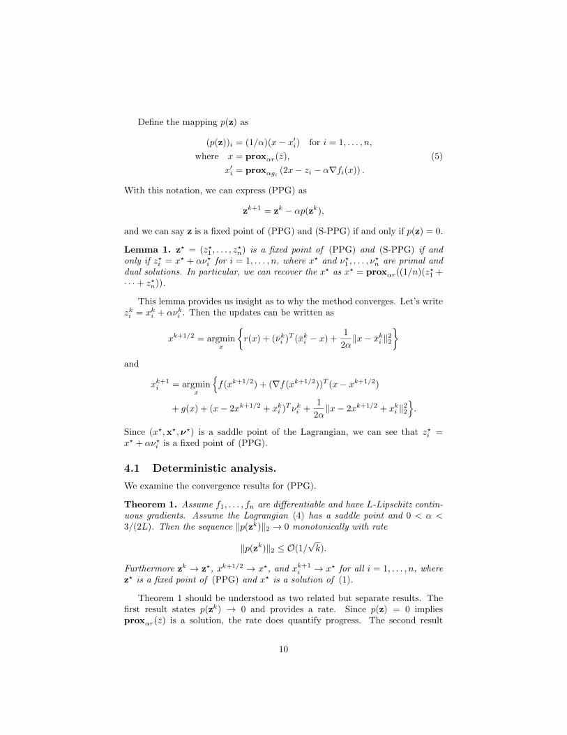
Define the mapping p(z) as
(p(z))i = (1/α)(x− x′i) for i = 1, . . . , n,
where x = proxαr(z), (5)
x′i = proxαgi (2x− zi − α∇fi(x)) .
With this notation, we can express (PPG) as
zk+1 = zk − αp(zk),
and we can say z is a fixed point of (PPG) and (S-PPG) if and only if p(z) = 0.
Lemma 1. z? = (z?1 , . . . , z?n) is a fixed point of (PPG) and (S-PPG) if and
only if z?i = x? + αν?i for i = 1, . . . , n, where x? and ν?1 , . . . , ν?n are primal and
dual solutions. In particular, we can recover the x? as x? = proxαr((1/n)(z?1 +· · ·+ z?n)).
This lemma provides us insight as to why the method converges. Let’s writezki = xki + ανki . Then the updates can be written as
xk+1/2 = argminx
r(x) + (νki )T (xki − x) +
1
2α‖x− xki ‖22
and
xk+1i = argmin
x
f(xk+1/2) + (∇f(xk+1/2))T (x− xk+1/2)
+ g(x) + (x− 2xk+1/2 + xki )T νki +1
2α‖x− 2xk+1/2 + xki ‖22
.
Since (x?,x?,ν?) is a saddle point of the Lagrangian, we can see that z?i =x? + αν?i is a fixed point of (PPG).
4.1 Deterministic analysis.
We examine the convergence results for (PPG).
Theorem 1. Assume f1, . . . , fn are differentiable and have L-Lipschitz contin-uous gradients. Assume the Lagrangian (4) has a saddle point and 0 < α <3/(2L). Then the sequence ‖p(zk)‖2 → 0 monotonically with rate
‖p(zk)‖2 ≤ O(1/√k).
Furthermore zk → z?, xk+1/2 → x?, and xk+1i → x? for all i = 1, . . . , n, where
z? is a fixed point of (PPG) and x? is a solution of (1).
Theorem 1 should be understood as two related but separate results. Thefirst result states p(zk) → 0 and provides a rate. Since p(z) = 0 impliesproxαr(z) is a solution, the rate does quantify progress. The second result
10

states that the iterates of (PPG) converge but with no guarantee of rate (justlike gradient descent without strong convexity).
To obtain a more direct measure of progress, define
Ek = r(xk+1/2) + f(xk+1/2) + g(xk+1)−(r(x?) + f(x?) + g(x?)
).
Ek is almost like the suboptimality of iterates, but not quite, as the point whereg is evaluated at is different from the point where r and f is evaluated at. Infact, Ek is not necessarily positive. Nevertheless, we can show a rate on |Ek|.
Theorem 2. Under the setting of Theorem 1,
|Ek| ≤ O(1/√k).
Define a similar quantity
ek =(r(xk+1/2) + f(xk+1/2) + g(xk+1/2)
)−(r(x?) + g(x?) + f(x?)
).
While ek truly measures suboptimality of xk+1/2, it is possible for ek = ∞ forall k = 1, 2, . . . because r and g are possibly nonsmooth and valued ∞ at somepoints. We need an additional assumption for ek to be a meaningful quantity.
Corollary 1. Assume the setting of Theorem 1. Further assume g(x) is Lips-chitz continuous with parameter Lg. Then
0 ≤ ek ≤ |Ek|+ Lg‖p(zk)‖
andek = O(1/
√k).
The proof of Corollary 1 follows immediately from combining Theorems 1and 2 with ek’s and Lg’s definitions.
The 1/√k rates for Theorem 2 and Corollary 1 can be improved to the 1/k
rates by using the ergodic iterates:
xk+1/2erg =
1
k
k∑j=1
xj+1/2, xk+1erg =
1
k
k∑j=1
xj+1.
With these ergodic iterates, we define
Ekerg =(r(xk+1/2
erg ) + f(xk+1/2erg ) + g(xk+1
erg ))−(r(x?) + g(x?) + f(x?)
),
ekerg =(r(xk+1/2
erg ) + f(xk+1/2erg ) + g(xk+1/2
erg ))−(r(x?) + g(x?) + f(x?)
).
Theorem 3. Assume the setting of Theorem 1. Then
|Ekerg| ≤ O(1/k)
Further assume g(x) is Lipschitz continuous with parameter Lg. Then
ekerg ≤ O(1/k).
11

Finally, under rather strong conditions on the problems, linear convergencecan also be shown.
Theorem 4. Assume the setting of Theorem 1. Furthermore, assume g isdifferentiable with Lipschitz continuous gradient. If one (or more) of r, g, or fis strongly convex, then (PPG) converges linearly in the sense that
‖zk − z?‖22 ≤ O(e−Ck)
for some C > 0. Consequently, |Ek| and ek also converge linearly.
4.2 Stochastic analysis.
As it turns out, the condition that guarantees (S-PPG) converges is the sameas that of (PPG). In particular, there is not step size reduction!
Theorem 5. Apply the same assumptions in Theorem 1. That is, assumef1, . . . , fn are differentiable and have L-Lipschitz continuous gradients, and as-sume the Lagrangian (4) has a saddle point and 0 < α < 3/(2L). Then thesequence ‖p(zk)‖2 → 0 with probability one at the rate
mini=0,...,k
E‖p(zi)‖22 ≤ O(1/k).
Furthermore zk → z?, xk+1/2 → x?, and xk+1i → x? for all i = 1, . . . , n with
probability one.
The expected objective rates of (S-PPG) also match those of (PPG).
Theorem 6. Under the same setting of Theorem 5, we have
E|Ek| ≤ O(1/√k) and |Ekerg| ≤ O(1/k). (6)
Further assume g(x) is Lipschitz continuous with parameter Lg. Then
Eekerg ≤ O(1/k).
Due to space limitation, we state without proof that, under the setting ofTheorem 4, (S-PPG) yields linearly convergent E‖zk − z?‖2, E|Ek|, and E|ek|.
5 Applications of PPG
To utilize (PPG), a given optimization problem often needs to be recast into theform of (1). In this section, we show some techniques for this while presentingsome interesting applications.
All examples presented in this section are naturally posed as
minimize r(x) +1
n
n∑i=1
fi(x) +1
m
m∑j=1
gj(x), (7)
12

where n 6= m. There is more than one way to recast Problem (7) into the formof Problem (1).
Among these options, the most symmetric one, loosely speaking, is
minimize r(x) +1
mn
n∑i=1
m∑j=1
(fi(x) + gj(x)
),
which leads to the method
xk+1/2 = proxαr
1
mn
n∑i=1
m∑j=1
zkij
xk+1ij = proxαgj
(2xk+1/2 − zkij − α∇fi(xk+1/2)
)zk+1ij = zkij + xk+1
ij − xk+1/2.
In general, the product mn can be quite large, and if so, this approach is likelyimpractical. In many examples, however, mn is not large as since n = 1 or mis small.
Another option, feasible when neither n nor m is small, is
minimize r(x) +1
m+ n
n∑i=1
((m+ n)/n)fi(x) +
m∑j=1
((m+ n)/m)gj(x)
,
which leads to the method
xk+1/2 = proxαr
1
n+m
n∑i=1
yki +
m∑j=1
zkj
yk+1i = xk+1/2 − α((m+ n)/n)∇fi(xk+1/2)
zk+1j = zkj − xk+1/2 + proxα((m+n)/m)gj
(2xk+1/2 − zkj
).
Overlapping group lasso. Let G be a collection of groups of indices. So G ⊆1, 2, . . . , d for each G ∈ G. The groups can be overlapping, i.e., G1 ∩G2 6= ∅is possible for G1, G2 ∈ G and G1 6= G2.
We let xG ∈ R|G| denote a subvector corresponding to the indices of G ∈ G,where x ∈ Rd is the whole vector. So the entries xi for i ∈ G form the vectorxG.
The overlapping group lasso problem is
minimize1
2‖Ax− b‖22 + λ1
∑G∈G‖xG‖2,
where x ∈ Rd is the optimization variable, A ∈ Rm×d and b ∈ Rm are problemdata, and λ1 > 0 is a regularization parameter. As it is, the regularizer (thesecond term) is not proximable when the groups overlap.
13

Partition the collection of groups G into n non-overlapping collections. SoG is a disjoint union of G1, . . . ,Gn, and if G1, G2 ∈ Gi and G1 6= G2 thenG1 ∩G2 = ∅ for i = 1, . . . , n. With some abuse of notation, we write
Gci = i ∈ 1, . . . , d | i /∈ G for all G ∈ Gi
Now we recast the problem into the form of (1)
minimize1
2‖Ax− b‖22 +
1
n
n∑i=1
(∑G∈Gi
λ2‖xG‖2
),
where λ2 = nλ1. The regularizer (the second term) is now a sum of n proximableterms.
For example, we can have a setup with d = 42, n = 3, G = G1 ∪G2 ∪G3, and
G1 = 1, . . . , 9, 10, . . . , 18, 19, . . . , 27, 28, . . . , 36G2 = 4, . . . , 12, 13, . . . , 21, 22, . . . , 30, 31, . . . , 39G3 = 7, . . . , 15, 16, . . . , 24, 25, . . . , 33, 34, . . . , 42
The groups within Gi do not overlap for each i = 1, 2, 3, and Gc2 = 1, 2, 3, 40, 41, 42.We view the first term as the r term, the second term as the sum of g1, . . . , gn,
and f1 = · · · = fn = 0 in the notation of (1), and apply (PPG):
xk+1/2 = (I + αATA)−1
(αAT b+
1
n
n∑i=1
zki
)zk+1/2i = 2xk+1/2 − zki
(xk+1i )G = uαλ2
((zk+1/2i )G
)for G ∈ Gi
(xk+1i )j = (z
k+1/2i )j for j ∈ Gci
zk+1i = zki + xk+1
i − xk+1/2,
where the indices i implicitly run through i = 1, . . . , n, and uα, defined in theSection 7, is the vector soft-thresholding operator.
To reduce the cost of computing xk+1/2, we can precompute and store theCholesky factorization of the positive definite matrix I + αATA (which costsO(m2d + d3)) and the matrix-vector product AT b (which costs O(md)). Thiscost is paid upfront once, and the subsequent iterations can be done inO(d2+dn)time.
For recent work on overlapping group lasso, see [68, 72, 27, 36, 32, 67, 25,10, 7, 64].
Low-rank and sparse matrix completion. Consider the setup where wepartially observe a matrix M ∈ Rd1×d2 on the set of indices Ω. More precisely,we observe Mij for (i, j) ∈ Ω while Mij for (i, j) /∈ Ω are unknown. We assumeM has a low-rank plus sparse structure, i.e., M = Ltrue + Strue with Ltrue is
14

low-rank and Strue is sparse. Here Ltrue models the true underlying structurewhile Strue models outliers. Furthermore, let’s assume 0 ≤Mij ≤ 1 for all (i, j).The goal is to estimate the unobserved entries of M , i.e., Mij for (i, j) /∈ Ω.
To estimate M , we solve the following regularized regression
minimize λ1‖L‖∗ + λ2‖S‖1 +∑
(i,j)∈Ω
`(Sij + Lij −Mij)
subject to 0 ≤ S + L ≤ 1,
where S,L ∈ Rd1×d2 are the optimization variables, the constraint 0 ≤ S +L ≤1 applies element-wise, and λ1, λ2 > 0 are regularization parameters. Theconstraint is proximable by Lemma 3, and we can use (PPG) either when `is differentiable or when `+ I[0,1] is proximable.
We view n = 1, the first term as the r term, the second term as the g1 term,and the last term as the f1 term in the notation of (1), and apply (PPG):
Lk+1/2 = tα(Zk)
Sk+1/2ij = sα
(Y kij)
for all (i, j)
Zk+1/2ij =
2L
k+1/2ij − Zkij for (i, j) /∈ Ω
2Lk+1/2ij − Zkij − α(L
k+1/2ij + S
k+1/2ij −Mij) for (i, j) ∈ Ω
Yk+1/2ij =
2S
k+1/2ij − Y kij for (i, j) /∈ Ω
2Sk+1/2ij − Y kij − α(L
k+1/2ij + S
k+1/2ij −Mij) for (i, j) ∈ Ω
Ak+1 = Zk+1/2 + Y k+1/2
Bk+1 = Zk+1/2 − Y k+1/2
Lk+1ij =
1
2
(Π[0,1](A
k+1ij ) +Bk+1
ij
)for all (i, j)
Sk+1ij =
1
2
(Π[0,1](A
k+1ij )−Bk+1
ij
)for all (i, j)
Zk+1 = Zk + Lk+1 − Lk+1/2
Y k+1 = Y k + Sk+1 − Sk+1/2.
tα and sα, defined in the Section 7, are respectively the matrix and scalar soft-thresholding operators. Π[0,1] is the projection onto the interval [0, 1], and the
Lk+1 and Sk+1 updates follow from Lemma 3. The only non-trivial operationfor this method is computing the SVD to evaluate tα
(Zk). All other operations
are elementary and embarrassingly parallel.For a discussion on low-rank + sparse factorization, see [9].
Regression with fused lasso. Consider the problem setup where we haveAxtrue = b and we observe A and b. Furthermore, the coordinates of xtrue areordered in a meaningful way and we know a priori that |xi+1 − xi| ≤ ε fori = 1, . . . , d− 1 and some ε > 0. finally, we also know that xtrue is sparse.
15

To estimate x, we solve the fused lasso problem
minimize λ‖x‖1 +1
n
n∑i=1
`i(x)
subject to |xi+1 − xi| ≤ ε, i = 1, . . . , d− 1
where`i(x) = (1/2)(aTi x− yi)2
and x ∈ Rd is the optimization variable.We recast the problem into the form of (1)
minimize λ‖x‖1
+1
2n
(n∑i=1
(`i(x) + go(x)) +
n∑i=1
(`i(x) + ge(x))
)
where
go(x) =∑
i=1,3,5,...
I[−ε,ε](xi+1 − xi)
ge(x) =∑
i=2,4,6,...
I[−ε,ε](xi+1 − xi)
and
I[−ε,ε](x) =
0 if |x| ≤ ε∞ otherwise.
Since go and ge are proximable by Lemma 3, we can apply (PPG).For recent work on fused lasso, see [57, 47, 58, 23, 33, 42, 66, 73].
Network lasso. Consider the problem setup where we have an undirectedgraph G = (E, V ). Each node v ∈ V has a parameter to estimate xv ∈ Rd andan associated loss function `v. Furthermore, we know that neighbors of G havesimilar parameters in the sense that ‖xu − xv‖2 is small if u, v ∈ E and thatxv is sparse for each v ∈ V .
Under this model, we solve the network lasso problem
minimize∑v∈V
λ1‖xv‖1 + `v(xv) +∑
u,v∈E
λ2‖xu − xv‖2,
where xv for all v ∈ V are the optimization variables, and `v(xv) for all v ∈ Va differentiable loss function, and λ1, λ2 > 0 are regularization parameters [22].
Say the G has an edge coloring E1, . . . , EC . So E1, . . . , EC partitions E suchthat if u, v ∈ Ec then u, v′ /∈ Ec for any v′ 6= v and c = 1, . . . , C. Figure 4illustrates this definition. (The chromatic index χ′(G) is the smallest possible
16

Figure 4: An edge coloring of the hypercube graph Q3.
value of C, but C need not be χ′(G).) With the edge coloring, we recast theproblem into the form of (1)
minimize∑v∈V
λ1‖xv‖1
+1
C
C∑c=1
∑v∈V
`v(xv) +∑
u,v∈Ec
λ3‖xu − xv‖2
,
where λ3 = Cλ2.We view the `1 regularizer as the r term, the loss functions as the f term,
and the summation over Ec as the g terms in the notation of (1), and apply(PPG):
xk+1/2v = sαλ1
(1
C
C∑c=1
zkcv
)zk+1/2cv = 2xk+1/2
v − zkcv − α∇`v(xk+1/2v )
skc = zk+1/2cu + zk+1/2
cv
dkc = zk+1/2cu − zk+1/2
cv
xk+1cu = skc + uαλ3
(dkc)
for u, v ∈ Ecxk+1cv = skc − uαλ3
(dkc)
for u, v ∈ Ecxk+1cv = zk+1/2
cv for v, u′ /∈ Ec for all u′ ∈ Vzk+1cv = zkcv + xk+1
cv − xk+1/2v ,
where the colors c implicitly run through c = 1, . . . , C unless specified otherwiseand the nodes v implicitly run through all v ∈ V . Here sα and uα, defined inthe Section 7, are respectively the scalar and vector soft-thresholding operators.
Although this algorithm, as stated, seemingly maintains C copies of xv wecan actually simplify it so that v maintains mindeg(v) + 1, C copies of xv forall v ∈ V . Since 2|E|/|V | is the average degree of G, storage requirement isO(|V |+ |E|) when simplified.
Let each node have a set N ⊆ 1, . . . , C such that c ∈ N if there is aneighbor connected through an edge with color c. Write N c = 1, . . . , C\N .
17

With this notation, we can rewrite the algorithm in a simpler, vertex-centricmanner:
FOR EACH node
x1/2 = sαλ1
(1
C
(|N c|zc′ +
∑c∈N
zkc
))FOR EACH color c ∈ Sz1/2c = 2x1/2 − zc − α∇f(x1/2)
Through edge with color c, send z1/2c and receive z′1/2c
s = z1/2c + z′1/2c
d = z1/2c − z′1/2c
xc = (1/2)(s+ uαλ2 (d))
zc = zc + xc − x1/2,
IF N c 6= ∅zc′ = x1/2 − α∇f(x1/2)
SVM. We solve the standard (primal) support vector machine setup [14]
minimizeλ
2‖x‖22 +
1
n
n∑i=1
gi(x), (8)
where x ∈ Rd is the optimization variable. The problem data is embedded in
gi(x) = max1− yiaTi x, 0
where λ > 0 is a regularization parameter and ai ∈ Rd, bi ∈ R and yi ∈ −1,+1are problem data for i = 1, . . . , n. Applying Lemma 2 and working out thedetails, we get a closed-form solution for the proximal operator:
proxαgi(x0) = x0 + Π[0,α]
(1− yiaTi x0
‖ai‖22
)yiai
for i = 1, . . . , n.We view r = (λ/2)‖x‖22 and f = 0 in the notation of (1), and apply (PPG):
xk+1/2 =1
1 + αλ
1
n
n∑i=1
zki
βki = yiΠ[0,α]
(1− yiaTi (2xk+1/2 − zki )
‖ai‖22
)zk+1i = xk+1/2 + βiai,
where the indices i implicitly run through i = 1, . . . , n.
18

Generalized linear model. In the setting of generalized linear models, themaximum likelihood estimator is the solution of the optimization problem
minimize1
n
n∑i=1
(A(xTi β)− TixTi β
),
where β ∈ Rd is the optimization variable, xi ∈ Rd and Ti ∈ R for i = 1, . . . , nare problem data, and A is a convex function on R.
We view r = 0, f = 0, and gi(β) = A(xTi β)− TixTi β in the notation of (1),and apply (PPG):
βk+1 =1
n
n∑i=1
zki
zk+1i = zki + proxαgi(2β
k − zki )− βk
where the indices i implicitly run from i = 1, . . . , n.For an introduction on generalized linear models, see [37].
Network Utility Maximization. In the problem of network utility maxi-mization, one solves the optimization problem
minimize (1/n)∑ni=1 fi(xi)
subject to xi ∈ Xi i = 1, . . . , nAixi ≤ y i = 1, . . . , ny ∈ Y,
where f1, . . . , fn are functions, A1, . . . , An are matrices, X1, . . . , Xn, Y are sets,and x1, . . . , xn, y are the optimization variables (For convenience, we convertthe maximization problem into a minimization problem.) For a comprehensivediscussion on network utility maximization, see [43].
This optimization problem is equivalent to the master problem
minimize1
n
n∑i=1
gi(y) + IY (y)
where we define the subproblems
gi(y) = inf fi(xi) |xi ∈ Xi, Aixi ≤ y ,
for i = 1, . . . , n. The master problem only involves the variable y, and xi is thevariable in the ith subproblem. For each i = 1, . . . , n, the function gi may notbe differentiable, but it is convex if fi and Xi are convex. If Y is convex, thenthe equivalent problem is convex.
19

0 50 100 150 200 250Iterations
10-8
10-4
100
Squ
are
dist
ance
to s
olut
ion Overlapping Group Lasso
ADMMPPGSPPG
Figure 5: The error ‖xk+1/2 − x?‖2 vs. iteration for overlapping group lassoexample.
We view f = 0 and r = IY in the notation of (1), and apply (PPG):
xk+1/2 = ΠY
(1
n
n∑i=1
zki
)
yk+1i = argmin
xi∈XiAixi≤yy∈Y
αfi(xi) +
1
2‖y − (2xk+1/2 − zki )‖22
zk+1i = zki + yk+1
i − yk+1/2.
Network utility maximization is often performed on a distributed computingnetwork, and if so the optimization problem for evaluating the proximal opera-tors can be solved in a distributed, parallel fashion.
6 Experiments
In this section, we present numerical experiments on two applications discussedin Section 5. The first experiment is small and is meant to serve as a proof ofconcept. The second experiment is more serious; the problem size is large andwe compare the performance with existing methods. For the sake of scientificreproducibility, we provide the code used to generate these experiments.
20

100 101 102 103 104
Epochs
10-8
10-6
10-4
10-2
100
Squ
are
dist
ance
to s
olut
ion SVM
PPGS-PPGSPI
Figure 6: The error ‖xk+1/2 − x?‖2 vs. iteration for the SVM example.
For both experiments, we observe linear convergence. This is a pleasantsurprise, as the theory presented in Section 4 and proved in Section 7 onlyguarantee a O(1/k) rate.
Overlapping group lasso. The problem size of this setup is m = 300, d = 42,n = 3. The groups are as described in Section 5.
The dominant cost per iteration of (PPG) is evaluating proxαr which takesO(d2) time with the precomputed factorization. Since the cost per iteration of(S-PPG) is no cheaper than that of (PPG), there is no reason to use (S-PPG).
We compare the performance of (PPG) to consensus ADMM (cf. §7.1 of[8]). Both methods use the same computational subroutines and therefore haveessentially the same computational cost per iteration. We show the results inFigure 5.
SVM. The problem size of this setup is n = 217 = 131, 072 and d = 512.The synthetic dataset A and y are randomly genearated and the regularizationparameter λ = 0.1 is used. So the problem data A consists of 64× 220 numbersand requires 500MB storage to store in double-precision floating-point format.
First, we compare the performance of (PPG) and (S-PPG) to the stochasticproximal iteration with diminishing step size αk = C/k in Figure 6. For allthree methods, the parameters were roughly tuned for optimal performance.
Next, we compare the (PPG) and (S-PPG) to a state-of-the-art SVM solver
21

Method Run time Objective valueLIBLINEAR 8.47s 3.7699CPU (PPG) 33.9s (30 iterations) 3.7364
CPU (S-PPG) 37.2s (30 epochs) 3.7364CUDA (PPG) 0.68s (30 iterations) 3.7364
Table 1: Run time as a function of grid size
LIBLINEAR [19]. Since LIBLINEAR is based on a second order method while(PPG) and (S-PPG) are first-order methods, comparing the number of iterationsis not very meaningful. Rather we compare the wall-clock time these methodstake to reach an equivalent level of accuracy. To compare the quality of thesolutions, we use the objective value of the problem (8).
The CPU code for (PPG) and (S-PPG) are written in C++. The codeis serial, not heaviliy optimized, and does not utilize BLAS (Basic Linear Al-gebra Subprograms) libraries or any SIMD instructions. On the other hand,LIBLINEAR is heavily optimized and does utilize BLAS.
We also implemented (PPG) on CUDA and ran it on a GPU. The algorith-mic structure of (PPG) is particularly well-suited for CUDA, especially whenthe problem size is large. Roughly speaking, the xk+1/2 update requires a re-duce operation, which can be done effectively on CUDA. The zki updates areembarassingly parallel, and can be done very effectively on CUDA. The threadsmust globally synchronize twice per iteration: once before computing the aver-age of zki for i = 1, . . . , n and once after xk+1/2 has been computed. Generallyspeaking, global synchronization on a GPU is expensive, but we have empiri-cally verified that the computational bottleneck is in the other operations, notthe synchronization, when the problem size is reasonably large.
Table 1 shows the results. We see that CPU implementation of (PPG)and (S-PPG) are competitive with LIBLINEAR, and could even be faster thanLIBLINEAR if the code is further optimized. On the other hand, the CUDA im-plementation of (PPG) clearly outperforms LIBLINEAR. (PPG) and (S-PPG)were run until the objective values were good as that of LIBLINEAR. Theseexpeirments were run on an Intel Core i7-990 GPU and a GeForce GTX TITANX GPU.
7 Convergence proofs
We say a function f is closed convex and proper if its epigraph(x, α) | x ∈ Rd, |f(x)| <∞, f(x) ≤ α
is a closed subset of Rd+1, f is convex, and f(x) = −∞ nowhere and f(x) <∞for some x.
22
A closed convex and proper function f has L-Lipschitz continuous gradientif f is differentiable everywhere and
‖∇f(x)−∇f(y)‖2 ≤ L‖x− y‖2
for all x, y ∈ Rd. This holds if and only if a closed convex and proper functionf satisfies
‖∇f(x)−∇f(y)‖22 ≤ L(∇f(x)−∇f(y))T (x− y)
for all x, y ∈ Rd, which is known as the Baillon-Haddad Theorem [2]. See[3, 4, 50] for a discussion on this.
Proximal operators are firmly non-expansive. This means for any closedconvex and proper function f and x, y ∈ Rd,
‖proxf (x)− proxf (y)‖22 ≤ (proxf (x)− proxf (y))T (x− y).
By applying Cauchy-Schwartz inequality, we can see that firmly non-expansiveoperators are non-expansive.
Some proximable functions. As discussed, many standard references like[11, 44] provide a list proximable functions. Here we discuss the few we use.
An optimization problem of the form
minimize f(x)subject to x ∈ C,
where x is the optimization variable and C is a constraint set, can be transformedinto the equivalent optimization problem
minimize f(x) + IC(x).
The indicator function IC is defined as
IC(x) =
0 for x ∈ C∞ otherwise,
and the proximal operator with respect to IC is
proxαIC (x) = ΠC(x)
where ΠC is the projection onto C for any α > 0. So IC is proximable if theprojection onto C is easy to evaluate.
The following results are well known. The proximal operator with respectto r(x) = |x| is called the scalar soft-thresholding operator
proxλr(x) = sλ(x) =
x+ λ x < −λ0 −λ ≤ x ≤ λx− λ x > λ.
23

The proximal operator with respect to r(x) = ‖x‖2 is called the vector soft-thresholding operator
proxλr(x) = uλ(x) =
max1− λ/‖x‖2, 0x for x 6= 00 otherwise.
The proximal operator with respect to r(M) = ‖M‖∗ is called the matrixsoft-thresholding operator
proxλr(M) = tλ(M) = Usλ(Σ)V T |UΣV T = M is the SVD,
where sλ(Σ) is applied element-wise to the diagonals.
Lemma 2. Assume g(x) = f(aTx) where a ∈ Rd and f is a closed, convex,and proper function on R. Then the proxg can be evaluated by solving a one-dimensional optimization problem.
Proof. By examining the optimization problem that defines proxg
proxg(x0) = argminx
f(aTx) +
1
2‖x− x0‖22
we see that solution must be of the form x0 + βa. So
proxg(x0) = x0 + βa, β = argminβ
f(aTx0 + β‖a‖22) +
‖a‖222
β2
.
Lemma 3. Let
g(x1, x2, . . . , xn) = f(a1x1 + a2x2 + · · ·+ anxn)
where x1, . . . , xn ∈ Rd, a ∈ Rn, a 6= 0, and f : R→ R ∪ ∞ is closed, convex,and proper. Then we can compute proxg with
w = prox‖a‖22f (a1ξ1 + a2ξ2 + · · ·+ anξn)
v =1
‖a‖22(a1ξ1 + a2ξ2 + · · ·+ anξn − w)
proxg(ξ1, ξ2, . . . , ξn) =
ξ1 − a1vξ2 − a2v
...ξn − anv
.
Proof. The optimality conditions of proxg(ξ1, ξ2, . . . , ξn) gives us
0 ∈ a21v + a1(x1 − ξ1)
......
0 ∈ a2nv + an(xn − ξn)
24

for some v ∈ ∂f(a1x1 + · · ·+ anxn). Summing this we get
0 ∈ ‖a‖22v + (a1x1 + · · ·+ anxn)− (a1ξ1 + · · ·+ anξn)
and with w = a1x1 + · · ·+ anxn we have
w = prox‖a‖22f (a1ξ1 + a2ξ2 + · · ·+ anξn).
The expression for v and proxg(ξ1, ξ2, . . . , ξn) follows from reorganizing theequations.
So if g(x, y) = f(x+ y) then
proxg(x0, y0) =1
2
(x0 − y0 + prox2f (x0 + y0)y0 − x0 + prox2f (x0 + y0)
).
If g(x, y) = f(x− y) then
proxg(x0, y0) =1
2
(x0 + y0 + prox2f (x0 − y0)x0 + y0 − prox2f (x0 − y0)
).
7.1 Deterministic analysis
Let h be a closed, convex, and proper function on Rd. When
x = proxαh(x0),
we haveαu+ x = x0
with u ∈ ∂h(x0). To simplify the notation, we write
α∇h(x0) + x = x0
where ∇h(x0) ∈ ∂h(x0). So is ∇h(x0) a subgradient of h at x0, and whichsubgradient ∇h(x0) is referring to depends on the context. (This notation isconvenient yet potentially sloppy, but we promise to not commit any fallacy ofequivocation.)
Proof of Lemma 1. Assume z? is a fixed point of (PPG) or (S-PPG). Thenp(z?) = 0. Then we have x? = x′?i for i = 1, . . . , n where x? and x′?1 , . . . , x
′?n are
as defined in (5). So
0 = α∇r(x?) + x? − z0 = α∇g1(x?)− x? + z?1 + α∇f1(x?)
......
0 = α∇gn(x?)− x? + z?n + α∇fn(x?).
25

Adding these up and dividing by n appropriately gives us
0 = ∇r(x?) + ∇g(x?) +∇f(x?),
so x? is a solution of Problem (1). Reorganize the definition of x in (5) to get
x? = argminx
r(x)− 1
α(z? − x?)Tx+
1
2α‖x− x?‖22
.
So x? minimizes L(·,x?, (1/α)(z? − x?)), where L is defined in (4). Reorganizethe definition of x′ in (5) to get
x? = argminx
f(x?) + (∇f(x?))T (x− x?) + g(x) +
1
α(z?i − x?)Tx+
1
2α‖x− x?‖22
.
So x? minimizes L(x?, ·, (1/α)(z? − x?)). So ν? = (1/α)(z? − x?) is a dualsolution of Problem (1).
The argument works in the other direction as well. If we assume (x?,ν?) isa primal dual solution of Problem (1), we can show that z? = x? + αν? is afixed point of (PPG) by following a similar line of logic.
Before we proceed to the main proofs, we introduce more notation. Definethe function
r(x) =1
n
n∑i=1
r(xi) + IC(x),
whereC = (x1, . . . , xn) |x1 = · · · = xn.
So
IC(x) =
0 for x1 = · · · = xn∞ otherwise.
As before, we write
f(x) =1
n
n∑i=1
fi(xi), g(x) =1
n
n∑i=1
gi(xi).
With this new notation, we can recast Problem (1) into
minimize r(x) + f(x) + g(x),
where x ∈ Rdn is the optimization variable. We can also rewrite the definition ofp as the following three-step process, which starts from z, produces intermediatepoints x,x′, and yields p(z):
x = proxαr(z) (9a)
x′ = proxαg(2x− z− α∇f(x)
)(9b)
p(z) = (1/α)(x− x′). (9c)
26

Note that x1, . . . , xn in x out of (9a) are identical due to IC . This is the samep as the p defined in (5); we’re just using the new notation.
We treat the boldface variables as vectors in Rdn. So the inner productbetween boldface variables is
xT z =
n∑i=1
xTi zi
and the gradient of f(x) is
∇f(x) =1
n
∇f1(x1)∇f2(x2)
...∇fn(xn)
.We use ∇g(x) and ∇r(x) in the same manner as before.
Lemma 4. Let z and z be any points in Rdn. Then
α‖p(z)− p(z)‖2 ≤ (p(z)− p(z))T (z− z)− (∇f(x)− f(x))T (x′ − x′)
where x and x′ are obtained by applying (9a) and then (9b), respectively, to zinstead of z.
Proof. This Lemma is similar to Lemma 3.3 of [15]. We reproduce the proofusing this paper’s notation.
‖z− αp(z)− z + αp(z)‖22(a)= ‖z− x− z + x‖22 + ‖x′ − x′‖22 + 2(z− x− z + x)T (x′ − x′)
(b)
≤ (z− x− z + x)T (z− z) + (x′ − x′)T (2x− z− α∇f(x)− 2x + z + α∇f(x))
+ 2(z− x− z + x)T (x′ − x′)
= (z− αp(z)− z + αp(z))T (z− z)− α(∇f(x)−∇f(x))T (x′ − x′),
where (a) is due to αp(z) = x−x′ and αp(z) = x− x′, (b) follows from the factthat the two mappings:
z 7→ z− x = z− proxαr(z)
and2x− z− α∇f(x) 7→ x′ = proxαg
(2x− z− α∇f(x)
)are both firmly non-expansive. By expanding the ‖z−αp(z)− z +αp(z)‖22 andcancellation, we obtain
‖αp(z)− αp(z)‖22 ≤ (αp(z)− αp(z))T (z− z)− α(∇f(x)−∇f(x))T (x′ − x′),
which proves the lemma by dividing both sides by α.
27

Lemma 5. Let z? be any fixed point of (PPG), i.e., p(z?) = 0. Then
‖zk − z?‖22 ≤ ‖z0 − z?‖22 (10)
for all k = 0, 1, . . . . Moreover, we have
∞∑k=0
‖p(zk)‖2 <∞ (11)
∞∑k=0
‖∇f(xk+1/2)−∇f(x?)‖2 <∞. (12)
Finally, ‖p(zk)‖2 monotonically decreases.
Proof. With the Baillon-Haddad theorem and Young’s inequality on (a) we get
−(∇f(x)−∇f(x))T (x′ − x′) (13)
= −(∇f(x)−∇f(x))T (x− αp(z)− x + αp(z)) (14)
= −(∇f(x)−∇f(x))T (x− x) + α(∇f(x)−∇f(x))T (p(z)− p(z)) (15)
(a)
≤ − 1L‖∇f(x)−∇f(x)‖2 + 3
4L‖∇f(x)−∇f(x)‖2 + Lα2
3 ‖p(z)− p(z)‖2(16)
= Lα2
3 ‖p(z)− p(z)‖2 − 14L‖∇f(x)−∇f(x)‖2. (17)
Combining Lemma 4 and equation (17), we obtain
−(p(z)− p(z))T (z− z) ≤ α(αL3 − 1)‖p(z)− p(z)‖2 − 14L‖∇f(x)−∇f(x)‖2.
(18)
Applying (18) separately with (z, z) = (zk, z?) and (zk, zk+1), we get, re-spectively,
‖zk+1 − z?‖2 = ‖zk − z?‖2 + α2‖p(zk)‖2 − 2α(zk − z?)T p(zk)
≤ ‖zk − z?‖2 − α2(1− 2αL3 )‖p(zk)‖2 − α
2L‖∇f(xk+1/2)−∇f(x?)‖2(19)
and
‖p(zk+1)‖2 = ‖p(zk)‖2 + ‖p(zk+1)− p(zk)‖2 − 2(p(zk+1)− p(zk))T 1α (zk+1 − zk)
≤ ‖p(zk)‖2 − (1− 2αL3 )‖p(zk+1)− p(zk)‖2. (20)
(In (17) we can use a different parameter for Young’s inequality, and improveinequalities (19) and (20) to allow α < 2/L, which is better than α < 3/(2L).In fact, α < 2/L is sufficient for convergence in Theorem 1. However, we usethe current version because we need the last term of inequality (19) for provingTheorem 3.)
Summing (19) through k = 0, 1, . . . give us the summability result. Inequal-ity (20) states that ‖p(zk)‖2 monotonically decreases.
28

Proof of Theorem 1. Lemma 5 already states that ‖p(zk)‖22 decreases monoton-ically. Using inequality (11) of Lemma 5, we get
‖p(zk)‖22 = mini=0,1,...,k
‖p(zi)‖22 ≤1
k
∞∑i=0
‖p(zi)‖22 = C/k = O(1/k)
for some finite constant C. (The rate O(1/k) can be improved to o(1/k) using,say, Lemma 1.2 of [18], but we present the simpler argument.)
By (10) of Lemma 5, zk is a bounded sequence and will have a limit point,which we call z∞. Lemma 4 also implies p is a continuous function. Sincep(zk) → 0 and p is continuous, the limit point z∞ must satisfy p(z∞) = 0.Applying inequality (10) with z? = z∞ tells us that ‖zk − z∞‖22 → 0, i.e., theentire sequence converges.
Since proxαr is a continuous function
xk+1/2 = proxαr(zk)→ proxαr(z
?) = x?.
With this same argument, we also conclude that xki → x? for all i = 1, . . . , n.
Proof of Theorem 2. A convex function h satisfies the inequality
h(x)− h(x) ≤ (∇h(x))T (x− x)
for any x and x (so long as a subgradient ∇h(x) exists).Applying this inequality we get
Ek ≤ (∇r(xk+1/2) +∇f(xk+1/2))T (xk+1/2 − x?) + (∇g(xk+1))T (xk+1 − x?)
= (∇r(xk+1/2) +∇f(xk+1/2) + ∇g(xk+1))T (xk+1/2 − x?)− (∇g(xk+1))T (αp(zk))
= (xk+1/2 − α∇g(xk+1)− x?)T p(zk) (21)
= ((zk+1 − z?) + α(∇r(x?) +∇f(xk+1/2)))T p(zk) (22)
= (zk+1 − z?)T p(zk) + α(∇r(x?) +∇f(xk+1/2))T p(zk). (23)
For the second equality, we used
p(zk) = ∇r(xk+1/2) +∇f(xk+1/2) + ∇g(xk+1).
and combined terms. For the third equality, we used x? = z? − α∇r(x?) and
xk+1/2−α∇f(xk+1/2)− α∇g(xk+1)
= zk − α∇r(xk+1/2)− α∇f(xk+1/2)− α∇g(xk+1)
= zk − αp(zk)
= zk+1.
Likewise we have
Ek ≥ (∇r(x?) +∇f(x?))T (xk+1/2 − x?) + (∇g(x?))T (xk+1 − x?)
= (xk+1 − x?)T p(z?) + (∇r(x?) +∇f(x?))Tαp(zk) (24)
= (∇r(x?) +∇f(x?))Tαp(zk). (25)
29

Here we usep(z?) = ∇r(x?) +∇f(x?) + ∇r(x?) = 0
Theorem 1 states that the sequences z1, z2, . . . and x1+1/2,x2+1/2, . . . bothconverge and therefore are bounded and that ‖p(zk)‖2 = O(1/
√k). Combining
this with the bounds on Ek gives us |Ek| ≤ O(1/√k).
Proof of Theorem 3. By Jensen’s inequality, we have
Ekerg ≤1
k
k∑i=1
Ei. (26)
Continuing the last line of (23), we get
Ek ≤ (zk+1 − z?)T p(zk) + α(∇r(x?) +∇f(xk+1/2))T p(zk) (27)
= 12α‖z
k − z?‖2 − 12α‖z
k+1 − z?‖2 − α2 ‖p(z
k)‖2 + α(∇r(x?) +∇f(xk+1/2))T p(zk).(28)
Combining (26) and (27) and after telescopic cancellation,
Ekerg ≤1
2αk‖z1 − z?‖2 +
1
k
k∑i=1
α(∇r(x?) +∇f(xi+1/2))T p(zi) (29)
= O(1/k) +1
kα(∇r(x?) +∇f(x?))T
k∑i=1
p(zi) +1
kα(∇f(xi)−∇f(x?))T
k∑i=1
p(zi)
(30)
≤ O(1/k) +1
kα‖zk+1 − z1‖‖∇r(x?) +∇f(x?)‖+
1
2k
k∑i=1
(α2‖p(zi)‖2 + ‖∇f(xi)−∇f(x?)‖2
)(31)
= O(1/k), (32)
where the last line holds due to the boundedness of zk and Lemma 5. With asimilar argument as in (25), we get
Ekerg ≥ (∇r(x?) +∇f(x?))T (xk+1/2erg − xk+1
erg ) =1
k
(k∑i=1
αp(zk)
)T(∇r(x?) +∇f(x?))
(33)
= 1k (zk − z0)T (∇r(x?) +∇f(x?)) = O(1/k), (34)
where have once again used the boundedness of (zk)k. Furthermore, since
|Ekerg − ekerg| ≤ Lg‖xk+1erg − xk+1/2
erg ‖ = Lg‖ 1k (zk+1 − z1)‖ = O(1/k), (35)
we have ekerg = O(1/k).
30

7.2 Stochastic analysis
Proof of Theorem 5. To express the updates of (S-PPG) we introduce the fol-lowing notation:
p(zk)[i] =
0...
p(zk)i...0
.
With this notation, we can express the iterates of (S-PPG) as
zk+1 = zk − αp(zk)[i(k)], (36)
and we also have conditional expectations
Ekp(zk)[i(k)] =1
np(zk),
Ek‖p(zk)[i(k)]‖2 =1
n‖p(zk)‖2.
Here, we let E denote the expectation over all random variables i(1), i(2), . . .,and Ek denote the expectation over i(k) conditioned on i(1), i(2), . . . , i(k − 1).
The convergence of this algorithm has been recently analyzed in [12] wheni(k) is chosen at random. Below, we adapt its proof to our setting with newrate results.
Note that Lemma 4 and inequality (17) remain valid, as they are not tiedto a specific sequence of random samples. Hence, similar to (19), we have
‖zk+1 − z∗‖2 = ‖zk − z∗‖2 + α2‖p(zk)[i(k)]‖2 − 2α(zk − z∗)T p(zk)[i(k)]. (37)
We take the conditional expectation to get
Ek‖zk+1 − z∗‖2 = ‖zk − z∗‖2 + α2Ek‖p(zk)[i(k)]‖2 − 2α(zk − z∗)TEkp(zk)[i(k)]
(38)= ‖zk − z∗‖2 + α2
n ‖p(zk)‖2 − 2α
n (zk − z∗)T p(zk) (39)
≤ ‖zk − z∗‖2 − α2
n (1− 2αL3 )‖p(zk)‖2 − α
2Ln‖∇f(xk)−∇f(x∗)‖2.(40)
By the same reasoning as before, we have
min0≤i≤k
E‖p(zk)‖2 ≤ O(1/k).
By (40), the sequence(‖zk − z∗‖2
)k≥0
is a nonnegative supermartingale. Ap-
plying Theorem 1 of [48] to (40) yields the following three properties, whichhold with probability one for every fixed point z?:
31

1. the squared fixed-point residual sequence is summable, that is,
∞∑k=0
‖p(zk)‖2 <∞, (41)
2. ‖zk − z∗‖2 converges to a nonnegative random number, and
3. (zk)k≥0 is bounded.
To proceed as before, however, we need ‖zk − z∗‖2 to converge to a nonneg-ative random number (not necessarily 0) for all fixed points z∗ with probabilityone. For each fixed point z∗, the previous argument states that there is a mea-sure one event set1, Ω(z∗), such that ‖zk − z∗‖2 converges for all (zk)k≥0 takenfrom Ω(z∗). Note that Ω(z∗) depends on z∗ because we must select z∗ to form(40) first. Since the number of fixed points (unless there is only one) is uncount-able, ∩fixed point z∗Ω(z∗) may not be measure one. Indeed, it is measure one aswe now argue.
Let Z∗ be the set of fixed points. Since Rdn is separable (i.e., containing acountable, dense subset), Z∗ has a countable dense subset, which we write asz∗1, z∗2, . . . . By countability, Ωc = ∩i=1,2,...Ω(z∗i ) is a measure one event set,and it is defined independently of the choice of z∗. Next we show that ‖zk−z∗‖2to converge to a nonnegative random number (not necessarily 0) for all fixedpoints z∗ with probability one by Ωc, that is, limk ‖zk−z∗‖ exists for all z∗ ∈ Z∗and all (zk)k≥0 ∈ Ωc.
Now consider any z∗ ∈ Z∗ and (zk)k≥0 ∈ Ωc. Then for any ε > 0, there is az∗i such that ‖z∗ − z∗i ‖ ≤ ε. By the triangle inequality, we can bound ‖zk − z∗‖as
‖zk − z∗‖ ≤ ‖zk − z∗i ‖+ ‖z∗i − z∗‖ ≤ ‖zk − z∗i ‖+ ε,
‖zk − z∗‖ ≥ ‖zk − z∗i ‖ − ‖z∗i − z∗‖ ≥ ‖zk − z∗i ‖ − ε.
Since ‖zk − z∗i ‖ converges, we have we have
lim supk‖zk − z∗‖ ≤ ε,
lim infk‖zk − z∗‖ ≥ −ε.
As ε > 0 is arbitrary, lim infk ‖zk− z∗‖ = lim supk ‖zk− z∗‖. So, limk ‖zk− z∗i ‖exists.
Finally, we can proceed with the same argument as in the proof of Theorem 1,and conclude that zk → z∗, xk+1/2 → x∗, and xk+1 → x∗ on the measure oneset Ωc.
1Each event is a randomly realized sequence of iterates (zk)k≥0 in S-PPG.
32
Proof of Theorem 6. This proof focuses on the treatments that are differentfrom the deterministic analysis. We only go through the steps of estimatingthe upper bound of E(Ek), skipping the similar treatment to obtain the lowerbound and other rates.
We reuse a part of (23) but avoid replacing zk − αp(zk) by zk+1 because of(36):
Ek ≤ (xk+1/2 − α∇g(xk+1)− x∗)T p(zk) (42)
= ((zk − αp(zk)− z∗) + α(∇r(x∗) +∇f(xk+1/2)))T p(zk) (43)
= (zk − αp(zk)− z∗)T p(zk) + α(∇r(x∗) +∇f(xk+1/2))T p(zk) (44)
= (zk − αp(zk)− z∗)T p(zk) + α(∇r(x∗) +∇f(x∗))T p(zk) (45)
+ α(∇f(xk+1/2)−∇f(x∗))T p(zk). (46)
By the Cauchy-Schwarz inequality,
E(Ek) ≤ E‖zk − αp(zk)− z∗‖ · E‖p(zk)‖+ α‖∇r(x∗) +∇f(x∗)‖ · E‖p(zk)‖
(47)
+ αE‖∇f(xk+1/2)−∇f(x∗)‖ · E‖p(zk)‖ (48)
≤(√
E‖zk − αp(zk)− z∗‖2 + α‖∇r(x∗) +∇f(x∗)‖ (49)
+ α√E‖∇f(xk+1/2)−∇f(x∗)‖2
)√E‖p(zk)‖2. (50)
Here we have√E‖zk − αp(zk)− z∗‖2 ≤
√‖z0 − z∗‖2 since, similar to (19),
‖zk − αp(zk)− z∗‖2 = ‖zk − z∗‖2 + α2‖p(zk)‖2 − 2α(zk − z∗)T p(zk)
≤ ‖zk − z∗‖2 − α2(1− 2αL3 )‖p(zk)‖2 − α
2L‖∇f(xk+1/2)−∇f(x∗)‖2
≤ ‖zk − z∗‖2 (51)
and, by (40), E‖zk − z∗‖2 ≤ E‖zk−1 − z∗‖2 ≤ · · · ≤ ‖z0 − z∗‖2. The next termin (50), α‖∇r(x∗) +∇f(x∗)‖, is a constant. For the third term, from
‖∇f(xk+1/2)−∇f(x∗)‖2(a)
≤ L2‖xk+1/2 − x∗‖2(b)
≤ L2‖zk − z∗‖2,
where (a) is due to Lipschitz continuity and (b) due to nonexpansiveness of the
proximal mapping, it follows that α√
E‖∇f(xk+1/2)−∇f(x∗)‖2 ≤ αL√‖z0 − z∗‖2.
Since E‖p(zk)‖2 = O(1/k), we immediately have E(Ek) ≤ O(1/√k). Similarly,
we can also show −E(Ek) ≤ O(1/√k). Therefore, E|Ek| = O(1/
√k).
By extending the previous analysis of |Ekerg| and ekerg to E|Ekerg| and E(ekerg),respectively, along the same line of arguments, it is straightforward to showE|Ekerg| = O(1/k) and E(ekerg) = O(1/k).
33

7.3 Linear convergence analysis
We first review some definitions and inequities. Let h be a closed convex properfunction. We let µh ≥ 0 be the strong-convexity constant of h, where µh > 0when h is strongly convex and µh = 0 otherwise. When h is differentiable and∇h is Lipschitz continuous, we define (1/βh) be the Lipschitz constant of ∇h.When h is either non-differentiable or differentiable but ∇h is not Lipschitz, wedefine βh = 0. Under these definitions, we have
h(y)−h(x)
≥ 〈∇h(x), y − x〉+1
2max
µh‖x− y‖2, βh‖∇h(x)− ∇f(y)‖2
︸ ︷︷ ︸
Sh(x,y)
, (52)
for any points x, y where the subgradients ∇h(x), ∇h(y) exist. Note thatSh(x, y) = Sh(y, x).
For the three convex functions r, f , g, we introduce their parameters µr, βr, µf , βf , µg, βg,as well as the combination
S(z, z∗) = Sr(x,x∗) + Sf (x,x∗) + Sg(x
′,x∗). (53)
As we assume each fi has L-Lipschitz gradient, we set βf = 1/L. Since rincludes the indicator function IC , which is non-differentiable, we set βr = 0.The values of remaining parameters µr, µf , µg, βg ≥ 0 are kept unspecified.Applying (52) to each pair of the three functions in
E =(r(x) + f(x) + g(x′)
)−(r(x∗) + f(x∗) + g(x∗)
)yields
E ≤ (∇r(x) +∇f(x))T (x− x∗) + (∇g(x′))T (x′ − x∗)− S(z, z∗), (54)
E ≥ (∇r(x∗) +∇f(x∗))T (x− x∗) + (∇g(x∗))T (x′ − x∗) + S(z, z∗). (55)
In this fashion, both the upper and lower bounds on Ek, which we previouslyderive, are tightened by S(zk, z∗). In particular, we can tightened (28) and (25)as
Ek ≤ 12α‖z
k − z∗‖2 − 12α‖z
k+1 − z∗‖2 − α2 ‖p(z
k)‖2 + α(∇r(x∗) +∇f(xk+1/2))T p(zk)− S(zk, z∗),(56)
Ek ≥ (∇r(x∗) +∇f(x∗))Tαp(zk) + S(zk, z∗), (57)
where the two terms involving S(zk, z∗) are newly added. Combining the upperand lower bounds of Ek yields
12α‖z
k+1 − z∗‖2 ≤ 12α‖z
k − z∗‖2 −Q, (58)
34

where
Q = −α(∇r(x∗) +∇f(xk+1/2))T p(zk) + α(∇r(x∗) +∇f(x∗))T p(zk) + α2 ‖p(z
k)‖2 + 2S(zk, z∗)
(59)
= −α(∇f(xk+1/2)−∇f(x∗))T p(zk) + α2 ‖p(z
k)‖2 + 2S(zk, z∗) (60)
=(− α(∇f(xk+1/2)−∇f(x∗))T p(zk) + α
2 ‖p(zk)‖2 + 2Sf (zk, z∗)
)+ 2Sr(z
k, z∗) + 2Sg(zk, z∗)
(61)
≥ c1(‖p(zk)‖2 + ‖∇f(xk+1/2)−∇f(x∗)‖2
)+µf2‖xk+1/2 − x?‖2 + 2Sr(z
k, z∗) + 2Sg(zk, z∗),
(62)
where c1 > 0 is a constant and the inequality follows from the Young’s inequal-ity:
α(∇f(xk+1/2)−∇f(x∗))T p(zk) ≤ α4 ‖p(z
k)‖2 + α‖∇f(xk+1/2)−∇f(x∗)‖2
and α < βf . Later on, in three different cases, we will show
Q ≥ C‖zk − z∗‖2. (63)
Hence, by substituting (63) into (58), we obtain the Q-linear (or quotient-linear)convergence relation
‖zk+1 − z∗‖ ≤√
1− 2αC‖zk − z∗‖, (64)
from which it is easy to further derive the Q-linear convergence results for |Ek|and ek.
Case 1. Assume g is both strongly convex and has Lipschitz gradient, i.e.,µg, βg > 0, (and f still has Lipschitz gradient). In this case,
Q = c1
(‖p(zk)‖2 + ‖∇f(xk+1/2)−∇f(x∗)‖2
)+ 2Sg(z
k, z∗) (65)
≥ c1(‖p(zk)‖2 + ‖∇f(xk+1/2)−∇f(x∗)‖2
)+ µg‖xk+1 − x?‖2. (66)
(Here we use ∇g instead of ∇g since g is differentiable.) By the identities
zk = xk+1 − α(∇g(xk+1) +∇f(xk+1/2)
)+ 2αp(zk), (67)
z∗ = x? − α(∇g(x?) +∇f(x?)
), (68)
the triangle inequality, and ‖∇g(xk+1)−∇g(x?)‖ ≤ (1/βg)‖xk+1−x?‖, we get
‖zk − z∗‖2 =∥∥(xk+1 − x?)− α
(∇g(xk+1)−∇g(x?)
)− α
(∇f(xk+1/2)−∇f(x?)
)+ 2αp(zk)
∥∥2
(69)
≤ 3∥∥(xk+1 − x?)− α
(∇g(xk+1)−∇g(x?)
)∥∥2+ 3α2‖∇f(xk+1/2)−∇f(x?)‖2 + 12α2‖p(zk)‖2
(70)
≤ 3(1 + αβg
)2‖xk+1 − x?‖2 + 3α2‖∇f(xk+1/2)−∇f(x?)‖2 + 12α2‖p(zk)‖2.(71)
35

Since (71) is bounded by (66) up to a constant factor, we have established (63)for this case.
Case 2. f is strongly convex and g has Lipschitz gradient, i.e., µf , βg > 0 (and
f still has Lipschitz gradient). In this case,
Q = c1
(‖p(zk)‖2 + ‖∇f(xk+1/2)−∇f(x∗)‖2
)+ µf‖xk+1/2 − x∗‖2. (72)
By the identities
zk = xk+1/2 − α(∇g(xk+1) +∇f(xk+1/2)
)+ αp(zk), (73)
z∗ = x? − α(∇g(x?) +∇f(x?)
), (74)
the triangle inequality, and ‖∇g(xk+1)−∇g(x?)‖ ≤ (1/βg)‖xk+1−x?‖, we get
‖zk − z∗‖2 =∥∥(xk+1/2 − x?)− α
(∇g(xk+1)−∇g(x?)
)− α
(∇f(xk+1/2)−∇f(x?)
)+ αp(zk)
∥∥2
(75)
≤ 4‖xk+1/2 − x?‖2 + 4α2‖∇g(xk+1)−∇g(x?)‖2 + 4α2‖∇f(xk+1/2)−∇f(x?)‖2 + 4α2‖p(zk)‖2(76)
≤ 4‖xk+1/2 − x?‖2 + 4α2
β2g‖xk+1 − x?‖2 + 4α2‖∇f(xk+1/2)−∇f(x?)‖2 + 4α2‖p(zk)‖2
(77)
≤ 4(1 + 2α2
β2g
)‖xk+1/2 − x?‖2 + 4α2‖∇f(xk+1/2)−∇f(x?)‖2 + 4α2(1 + 2α2
β2g
)‖p(zk)‖2,(78)
where the last line follows from
‖xk+1 − x?‖2 = ‖xk+1/2 − x? − αp(zk)‖2 ≤ 2‖xk+1/2 − x?‖2 + 2α2‖p(zk)‖2.
Since (78) is bounded by (72) up to a constant factor, we have established (63)for this case.
Case 3. r is strongly convex and g has Lipschitz gradient, in short, µrβg > 0,(and f still has Lipschitz gradient). In this case,
Q = c1
(‖p(zk)‖2 + ‖∇f(xk+1/2)−∇f(x∗)‖2
)+ µr‖xk+1/2 − x∗‖2. (79)
We still use (78), which is bounded by (79) up to a constant factor, we haveestablished (63) for this case.
8 Conclusion and future work
In this paper we presented (PPG) and a variant (S-PPG). By discussing possi-ble applications, we demonstrated how (PPG) expands the class of optimization
36

problems that can be solved with a simple and scalable method. We proved con-vergence and demonstrated the effectiveness, especially in parallel computing,of the methods through computational experiments.
An interesting future direction is to consider cyclic and asynchronous vari-ations of (PPG). Generally speaking, random coordinate updates can be com-putationally inefficient, and cyclic coordinate updates access the data more ef-ficiently. (PPG) is a synchronous algorithm; at each iteration the z1, . . . , zn areupdated synchronously and the synchronization can cause inefficiency. Asyn-chronous updates avoid this problem.
References
[1] T. Arjevani and O. Shamir. Communication complexity of distributedconvex learning and optimization. In NIPS, pages 1756–1764. 2015.
[2] J.-B. Baillon and G. Haddad. Quelques proprietes des operateurs angle-bornes et n-cycliquement monotones. Israel Journal of Mathematics,26(2):137–150, 1977.
[3] H. H. Bauschke and P. L. Combettes. The Baillon-Haddad Theorem Re-visited, 17(3–4):781–787, 2010.
[4] H. H. Bauschke and P. L. Combettes. Convex Analysis and MonotoneOperator Theory in Hilbert Spaces. 2011.
[5] D. P. Bertsekas. Incremental proximal methods for large scale convex op-timization. Mathematical Programming, 129(2):163–195, 2011.
[6] P. Bianchi. Ergodic convergence of a stochastic proximal point algorithm.SIAM Journal on Optimization, 26(4):2235–2260, 2016.
[7] J. Bien, J. Taylor, and R. Tibshirani. A lasso for hierarchical interactions.The Annals of Statistics, 41(3):1111–1141, 2013.
[8] S. Boyd, N. Parikh, E. Chu, B. Peleato, and J. Eckstein. Distributedoptimization and statistical learning via the alternating direction methodof multipliers. Foundations and Trends in Machine Learning, 3(1):1–122,2011.
[9] V. Chandrasekaran, S. Sanghavi, P. A. Parrilo, and A. S. Willsky. Rank-sparsity incoherence for matrix decomposition. SIAM Journal on Opti-mization, 21(2):572–596, 2011.
[10] X. Chen, Q. Lin, S. Kim, J. G. Carbonell, and E. P. Xing. Smoothingproximal gradient method for general structured sparse regression. TheAnnals of Applied Statistics, 6(2):719–752, 2012.
[11] P. L. Combettes and J.-C. Pesquet. Proximal Splitting Methods in SignalProcessing, pages 185–212. 2011.
37

[12] P. L. Combettes and J.-C. Pesquet. Stochastic quasi-Fejer block-coordinatefixed point iterations with random sweeping. SIAM Journal on Optimiza-tion, 25(2):1221–1248, 2015.
[13] P. L. Combettes and V. R. Wajs. Signal recovery by proximal forward-backward splitting. Multiscale Modeling and Simulation, 4(4):1168–1200,2005.
[14] C. Cortes and V. Vapnik. Support-vector networks. Machine Learning,20(3):273–297, 1995.
[15] Damek Davis and Wotao Yin. A three-operator splitting scheme and itsoptimization applications. Set-Valued and Variational Analysis, Jun 2017.
[16] A. Defazio, F. Bach, and A. Lacoste-Julien. SAGA: A fast incremental gra-dient method with support for non-strongly convex composite objectives.In NIPS, pages 1646–1654. 2014.
[17] A. Defazio, J. Domke, and T. S. Caetano. Finito: A faster, permutableincremental gradient method for big data problems. In ICML, volume 32,pages 1125–1133, 2014.
[18] W. Deng, M.-J. Lai, Z. Peng, and W. Yin. Parallel multi-block ADMMwith o(1/k) convergence. Journal of Scientific Computing, 2016.
[19] R.-E. Fan, K.-W. Chang, C.-J. Hsieh, X.-R. Wang, and C.-J. Lin. LIBLIN-EAR: A library for large linear classification. Journal of Machine LearningResearch, 9:1871–1874, 2008.
[20] D. Gabay and B. Mercier. A dual algorithm for the solution of nonlin-ear variational problems via finite element approximation. Computers andMathematics with Applications, 2(1):17–40, 1976.
[21] R. Glowinski and A. Marroco. Sur l’approximation, par elements finisd’ordre un, et la resolution, par penalisation-dualite d’une classe de prob-lmes de Dirichlet non lineaires. Revue Francaise d’Automatique, Informa-tique, Recherche Operationnelle. Analyse Numerique, 9(2):41–76, 1975.
[22] D. Hallac, J. Leskovec, and S. Boyd. Network lasso: Clustering and opti-mization in large graphs. In KDD, pages 387–396, 2015.
[23] H. Hoefling. A path algorithm for the fused lasso signal approximator.Journal of Computational and Graphical Statistics, 19(4):984–1006, 2010.
[24] M. Jaggi, V. Smith, M. Takac, J. Terhorst, S. Krishnan, T. Hofmann, andM. I. Jordan. Communication-efficient distributed dual coordinate ascent.In NIPS. 2014.
[25] R. Jenatton, J.-Y. Audibert, and F. Bach. Structured variable selectionwith sparsity-inducing norms. Journal of Machine Learning Research,12:2777–2824, 2011.
38

[26] R. Johnson and T. Zhang. Accelerating stochastic gradient descent usingpredictive variance reduction. In NIPS, pages 315–323. 2013.
[27] S. Kim and E. P. Xing. Tree-guided group lasso for multi-task regressionwith structured sparsity. In ICML, pages 543–550, 2010.
[28] B. Kulis and P. L. Bartlett. Implicit online learning. In ICML, pages575–582, 2010.
[29] G. Lan and Y. Zhou. An optimal randomized incremental gradient method.2015.
[30] J. Langford, L. Li, and T. Zhang. Sparse online learning via truncatedgradient. Journal of Machine Learning Research, 10:777–801, 2009.
[31] N. Le Roux, M. Schmidt, and F. Bach. Stochastic gradient method withan exponential convergence rate for finite training sets. In NIPS, 2012.
[32] J. Liu and J. Ye. Moreau-Yosida regularization for grouped tree structurelearning. In NIPS, pages 1459–1467. 2010.
[33] J. Liu, L. Yuan, and J. Ye. An efficient algorithm for a class of fused lassoproblems. In KDD, pages 323–332. 2010.
[34] J. Mairal. Optimization with first-order surrogate functions. In ICML,pages 783–791, 2013.
[35] J. Mairal. Incremental majorization-minimization optimization with ap-plication to large-scale machine learning. SIAM Journal on Optimization,25(2):829–855, 2015.
[36] J. Mairal, R. Jenatton, F. R. Bach, and G. R. Obozinski. Network flowalgorithms for structured sparsity. In NIPS, pages 1558–1566. 2010.
[37] P. McCullagh and J. A. Nelder. Generalized linear models. 2nd edition,1989.
[38] H. B. McMahan. Follow-the-regularized-leader and mirror descent: Equiv-alence theorems and l1 regularization. In AISTATS, 2011.
[39] G. J. Minty. Monotone (nonlinear) operators in Hilbert space. Duke Math-ematical Journal, 29(3):341–346, 1962.
[40] J. F. C. Mota, J. M. F. Xavier, P. M. Q. Aguiar, and M. Puschel. D-ADMM: A communication-efficient distributed algorithm for separable op-timization. IEEE Transactions on Signal Processing, 61(10):2718–2723,2013.
[41] A. Nitanda. Stochastic proximal gradient descent with acceleration tech-niques. In NIPS, pages 1574–1582. 2014.
39

[42] G. Nowak, T. Hastie, J. R. Pollack, and R. Tibshirani. A fused lassolatent feature model for analyzing multi-sample aCGH data. Biostatistics,12(4):776–791, 2011.
[43] D. P. Palomar and M. Chiang. Alternative distributed algorithms for net-work utility maximization: Framework and applications. IEEE Transac-tions on Automatic Control, 52(12):2254–2269, 2007.
[44] N. Parikh and S. Boyd. Proximal algorithms. Foundations and Trends inOptimization, 1(3):127–239, 2014.
[45] G. B. Passty. Ergodic convergence to a zero of the sum of monotone oper-ators in Hilbert space. Journal of Mathematical Analysis and Applications,72(2):383–390, 1979.
[46] H. Raguet, J. Fadili, and G. Peyre. A generalized forward-backward split-ting. SIAM Journal on Imaging Sciences, 6(3):1199–1226, 2013.
[47] F. Rapaport, E. Barillot, and J.-P. Vert. Classification of arrayCGH datausing fused SVM. Bioinformatics, 24(13):i375–i382, 2008.
[48] H. Robbins and D. Siegmund. A convergence theorem for non negative al-most supermartingales and some applications. In Herbert Robbins SelectedPapers, pages 111–135. 1985.
[49] E. K. Ryu and S. Boyd. Stochastic proximal iteration: A non-asymptoticimprovement upon stochastic gradient descent. 2014.
[50] E. K. Ryu and S. Boyd. Primer on monotone operator methods. Appliedand Computational Mathematics, 15(1):3–43, 2016.
[51] A. Salim, P. Bianchi, W. Hachem, and J. Jakubowicz. A stochastic proximalpoint algorithm for total variation regularization over large scale graphs.In IEEE CDC, pages 4490–4495, 2016.
[52] M. Schmidt, N. Le Roux, and F. Bach. Minimizing finite sums with thestochastic average gradient. Mathematical Programming, pages 1–30, 2016.
[53] S. Shalev-Shwartz. SDCA without duality, regularization and individualconvexity. In ICML, pages 747–754, 2016.
[54] S. Shalev-Shwartz and T. Zhang. Stochastic dual coordinate ascent meth-ods for regularized loss. Journal of Machine Learning Research, 14:567–599,2013.
[55] S. Shalev-Shwartz and T. Zhang. Accelerated proximal stochastic dual co-ordinate ascent for regularized loss minimization. Mathematical Program-ming, 155(1):105–145, 2016.
[56] O. Shamir, N. Srebro, and T. Zhang. Communication-efficient distributedoptimization using an approximate Newton-type method. In ICML, 2014.
40

[57] R. Tibshirani, M. Saunders, S. Rosset, J. Zhu, and K. Knight. Sparsity andsmoothness via the fused lasso. Journal of the Royal Statistical Society:Series B, 67(1):91–108, 2005.
[58] R. Tibshirani and P. Wang. Spatial smoothing and hot spot detection forCGH data using the fused lasso. Biostatistics, 9(1):18, 2008.
[59] P. Toulis and E. M. Airoldi. Asymptotic and finite-sample properties ofestimators based on stochastic gradients. Annals of Statistics (To appear),2017.
[60] P. Toulis, J. Rennie, and E. M. Airoldi. Statistical analysis of stochasticgradient methods for generalized linear models. In ICML, pages 667–675,2014.
[61] M. Wang and D. P. Bertsekas. Incremental constraint projection methodsfor variational inequalities. Mathematical Programming, 150(2):321–363,2015.
[62] M. Wang and D. P. Bertsekas. Stochastic first-order methods with randomconstraint projection. SIAM Journal on Optimization, 26(1):681–717, 2016.
[63] L. Xiao and T. Zhang. A proximal stochastic gradient method with progres-sive variance reduction. SIAM Journal on Optimization, 24(4):2057–2075,2014.
[64] E. Yang, A. Lozano, and P. Ravikumar. Elementary estimators for high-dimensional linear regression. In ICML, pages 388–396, 2014.
[65] T. Yang. Trading computation for communication: Distributed stochasticdual coordinate ascent. In NIPS. 2013.
[66] G.-B. Ye and X. Xie. Split Bregman method for large scale fused lasso.Computational Statistics & Data Analysis, 55(4):1552–1569, 2011.
[67] L. Yuan, J. Liu, and J. Ye. Efficient methods for overlapping group lasso.In NIPS, pages 352–360. 2011.
[68] M. Yuan and Y. Lin. Model selection and estimation in regression withgrouped variables. Journal of the Royal Statistical Society: Series B,68(1):49–67, 2006.
[69] L. Zhang, M. Mahdavi, and R. Jin. Linear convergence with conditionnumber independent access of full gradients. In NIPS, pages 980–988. 2013.
[70] Y. Zhang and L. Lin. Disco: Distributed optimization for self-concordantempirical loss. In ICML, 2015.
[71] Y. Zhang, M. J. Wainwright, and J. C. Duchi. Communication-efficientalgorithms for statistical optimization. In NIPS, pages 1502–1510. 2012.
41

[72] P. Zhao, G. Rocha, and B. Yu. The composite absolute penalties familyfor grouped and hierarchical variable selection. The Annals of Statistics,(6A):3468–3497, 2009.
[73] J. Zhou, J. Liu, V. A. Narayan, and J. Ye. Modeling disease progressionvia fused sparse group lasso. In KDD, pages 1095–1103. 2012.
42