Embed Size (px)
Citation preview

Eric W. Lemmon
Applied Chemicals and Materials DivisionNational Institute of Standards and Technology
Boulder, Colorado


Vapor Phase
Liquid Phase
Critical region Accuracy Speed Iteration
Ideal gas law √ Low High Novan der Waals √ √ √ Low High NoCubics √ √ √ Moderate High NoVirials √ Moderate Med YesBWRs √ √ √ High Med YesHelmholtz √ √ √ Very High Low Yes
Each calculates pressure as a function of density and temperature, except for the Helmholtz energy equation.
EOS Characteristics

=Doesn’t it?

=1 =Z(for an ideal gas)

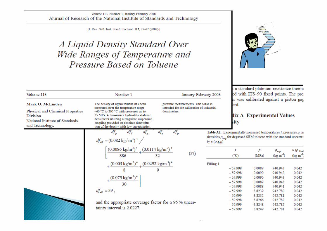
Z=1+B
Z=1+B+C2B Second virial coefficientC Third virial coefficient

Z-1 =B+C+D2
Z=1+B+C2+D3

Z=1+B (Z-1)/=B
B(300 K)=-0.645

Z=1+B+C2 (Z-1)/=B+C
B(300 K)=-0.645
2.0
C(300 K)=-0.033
0.066

Z=1+B+C2+D3
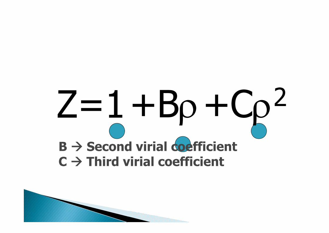
Full Equation of State – R-125

Full Equation of State – R-125

Peng-Robinson EOS for Nitrogen

Why not just use pressure for the independent variable in our equation of state?
T
pRT
RTT
RTu
2
20
2
1ln
Equations of State

All thermodynamic properties can be calculated as derivatives from each of the four fundamental equations:
Internal energy as a function of density and entropy◦ Entropy is not a measurable quantity.
Enthalpy as a function of pressure and entropy◦ Entropy is not a measurable quantity. Cannot have a
continuous equation across the phase boundary. Gibbs energy as a function of pressure and temperature◦ Cannot have a continuous equation across the phase boundary.
Helmholtz energy as a function of temperature and density◦ Both temperature and density are measurable. Continuous
across two-phase region.
Types of Fundamental Equations
All thermodynamic properties can be calculated as derivatives from each of the four fundamental equations:
Enthalpy as a function of pressure and entropy◦ Entropy is not a measurable quantity. Is not continuous from
liquid to vapor states.
Gibbs energy as a function of pressure and temperature◦ Cannot have a continuous equation across the phase boundary.
Helmholtz energy as a function of temperature and density◦ Both temperature and density are measurable. Continuous
across two-phase region.
Types of Fundamental Equations

All thermodynamic properties can be calculated as derivatives from each of the four fundamental equations:
Gibbs energy as a function of pressure and temperature◦ Is not continuous from liquid to vapor states.
Helmholtz energy as a function of temperature and density◦ Both temperature and density are measurable. Continuous
across two-phase region. Internal energy as a function of density and entropy◦ Entropy is not a measurable quantity.
Enthalpy as a function of pressure and entropy◦ Entropy is not a measurable quantity. Cannot have a
continuous equation across the phase boundary.
Types of Fundamental Equations
All thermodynamic properties can be calculated as derivatives from each of the four fundamental equations:
Helmholtz energy as a function of temperature and density◦ Both temperature and density are measurable. Continuous
across two-phase region. Internal energy as a function of density and entropy◦ Entropy is not a measurable quantity.
Enthalpy as a function of pressure and entropy◦ Entropy is not a measurable quantity. Cannot have a
continuous equation across the phase boundary. Gibbs energy as a function of pressure and temperature◦ Cannot have a continuous equation across the phase boundary.
Types of Fundamental Equations

ap 2
TaTau
Tas
Why the Helmholtz Energy is Best

Who is Helmholtz?
Hermann Ludwig Ferdinand von Helmholtz (1821 – 1894)

ideal
2
22
RCV
Helmholtz Energy Equation of State
22exp kkkkdt
k aN kk
jjj ldtjN exp
TTcritcrit
r
1RTp
Polynomial terms
Polynomial+exponential terms
Other properties as derivatives only
Reduced independent variables
ii dtiN
Gaussian bell-shaped terms
Ideal gas

Ideal gas heat capacity data Pressure-density-temperature data Vapor pressure data Speed of sound data Heat capacity data Virial coefficients etc.
Data Needed for Fitting Equations of State

Reference equations of state with very low uncertainties are available for the few but well characterized fluids.
A number of fluids have adequate data to make good equations, and most of these have been published.
The rest have little or no data above the critical point, and often no PVT data in the vapor phase.◦ Extrapolation without constraints and visual observations will lead
to poor equations. In all cases, even the most well measured substances
can go astray at very high densities.
Typical Data Available
Linear fitting of data only with a bank of terms –no graphical examination of behavior.
Same linear fitting of data but with graphical inspection of equation – bad extrapolation fixed with “graphite research”.
Combination of linear and nonlinear fitting. Pure nonlinear fitting of data only (with
graphical assessment of extrapolation). Nonlinear fitting combined with
multiple constraints to control curvature of different properties.
`
History of Equations of State

Graphite Research

Early fitting programs only looked at statistics. Modern functional forms are extremely flexible and can
fit any kind of data – good or bad. The statistics can show that an equation does a
wonderful job fitting the good (and bad) data, but only a full inspection of the behavior of the equation will validate its accuracy.
The correlator must have good knowledge of the behavior of a fluid to remove bad performance, becoming an Artist by “painting” the fluid’s shape.
Fitting: Art vs. Statistics

Fitting Equations of State IS an Art
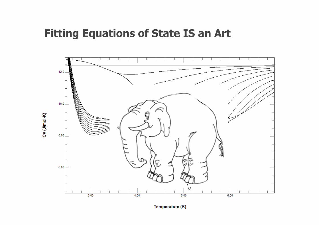
Fitting Equations of State IS an Art
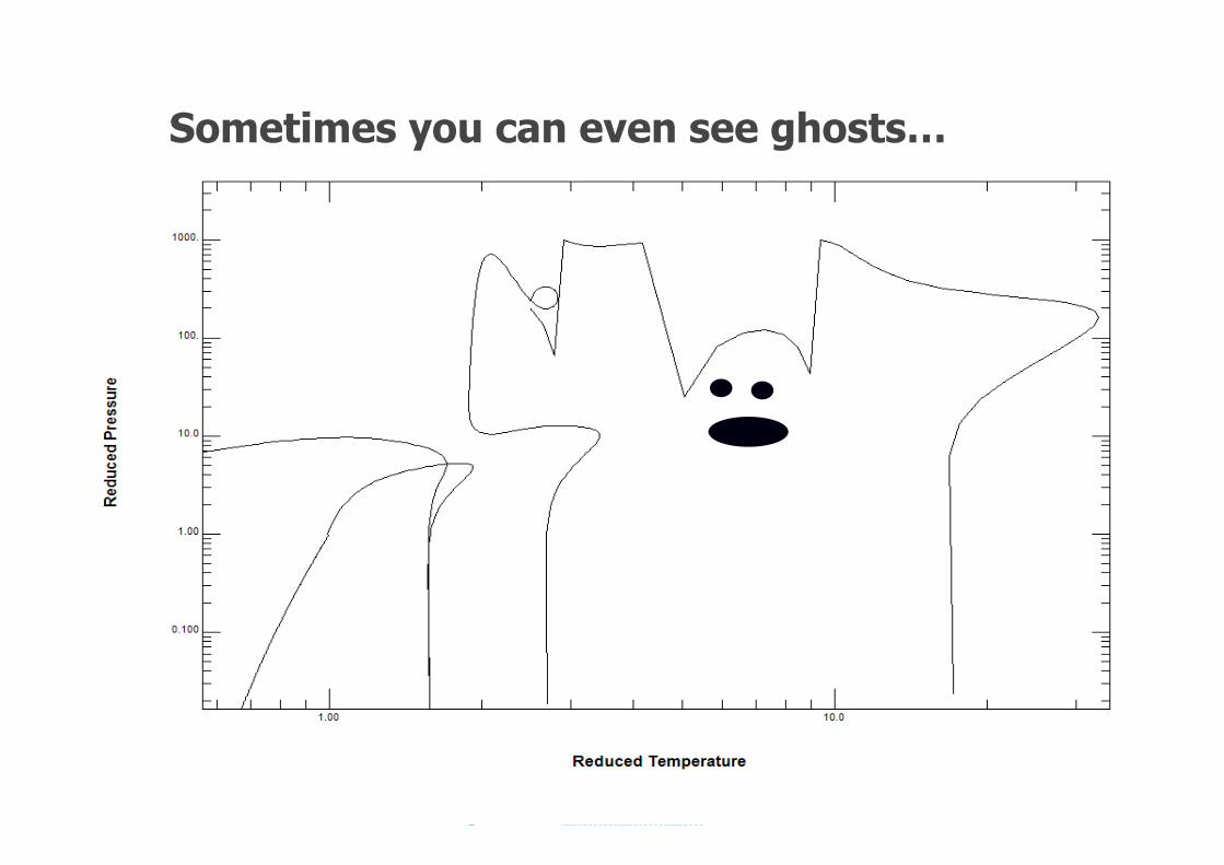
Sometimes you can even see ghosts…

Linear fitting◦ Fast.◦ Selects optimum terms from a large bank.◦ Can fit multiple properties simultaneously,
but isobaric heat capacity, sound speed, and phase boundary data must be linearized with a preliminary equation.
◦ Final equations have 25-50 terms. Nonlinear fitting◦ Very time consuming.◦ Can fit multiple properties simultaneously
without the need to linearize.◦ Final equations have 15-25 terms.
Techniques Used in Fitting

R-134a
Wow!!!
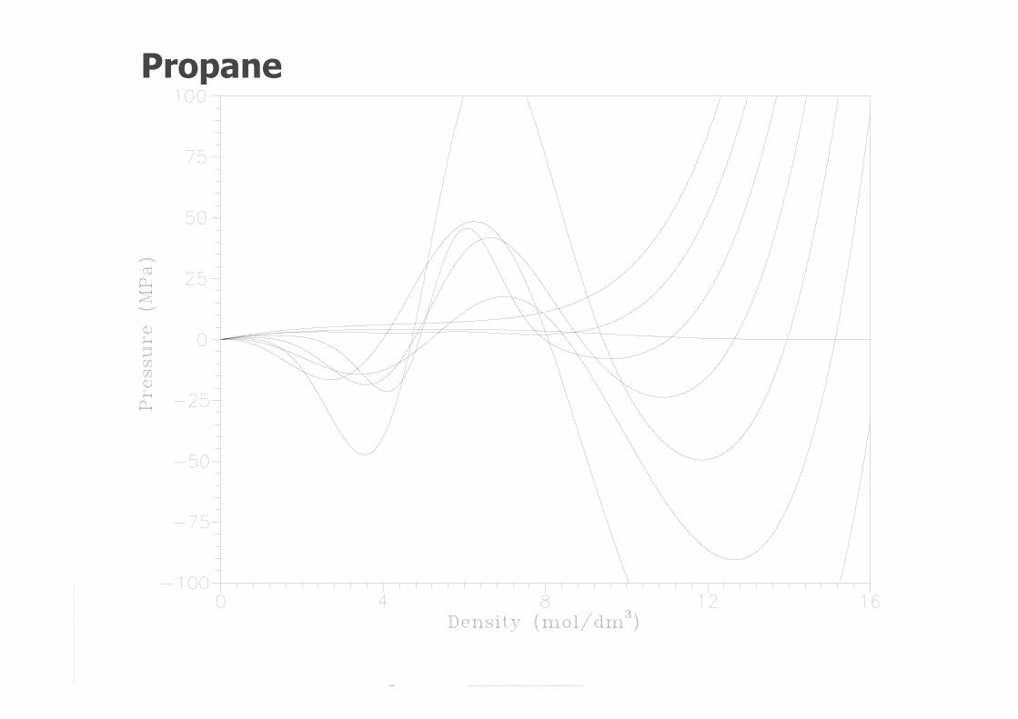
Propane

Nonlinear fitting can include the exponents on density and temperature, as well as the coefficients and exponents within the Gaussian-bell shaped terms.
Nonlinear fitting can use greater than and less than concepts to shape an equation in the absence of data, such as:◦ Make cv increase in value as temperature drops to low values in the liquid
phase.◦ Force a temperature exponent to be less than a particular value.◦ Keep the critical density or temperature within a set bound (when it is
fitted).◦ Calculate the rectilinear diameter and keep it straight (no curvature).◦ Smooth out the ideal curves.
Nonlinear Fitting

R-143a

R-125

CV/DT/S+
Property to shape
Property held constant
Property varied
Derivative to fitCan be one of four:S – SlopeC – Curvature3 – 3rd derivative4 – 4th derivative
What to do with the derivative:+ Make it positive– Make it negative0 Make it zero& Allow only one cross from negative to positive
Fitting Constraints

2PD/ST/A-+ C/DL/A& CV/ST/A+ JI/TD/C0 P/TD/A+ RD/ST/C0 W/ST/A- Z1/ST/A+-
Make the second derivative along the saturation line have a negative slope, positive curvature, negative 3rd, and positive 4th .
Calculate C on a log temperature scale, allowing each derivative to pass through zero once only.
Keep all derivatives of Cv along the saturation line positive.
Keep the curvature along the Joule Inversion curve zero as the density is increased.
Along an isotherm, force all pressure derivatives to be positive while varying density.
Make the rectilinear diameter straight, with no curvature.
Force the derivatives of the speed of sound to all have negative derivatives along the saturation curve.
Along the saturation line, make the derivatives (Z-1)/rho positive for the slope, negative for the curvature, positive for the 3rd, and negative for the 4th.
Constraint Examples


Snapshot of EOS Fitting
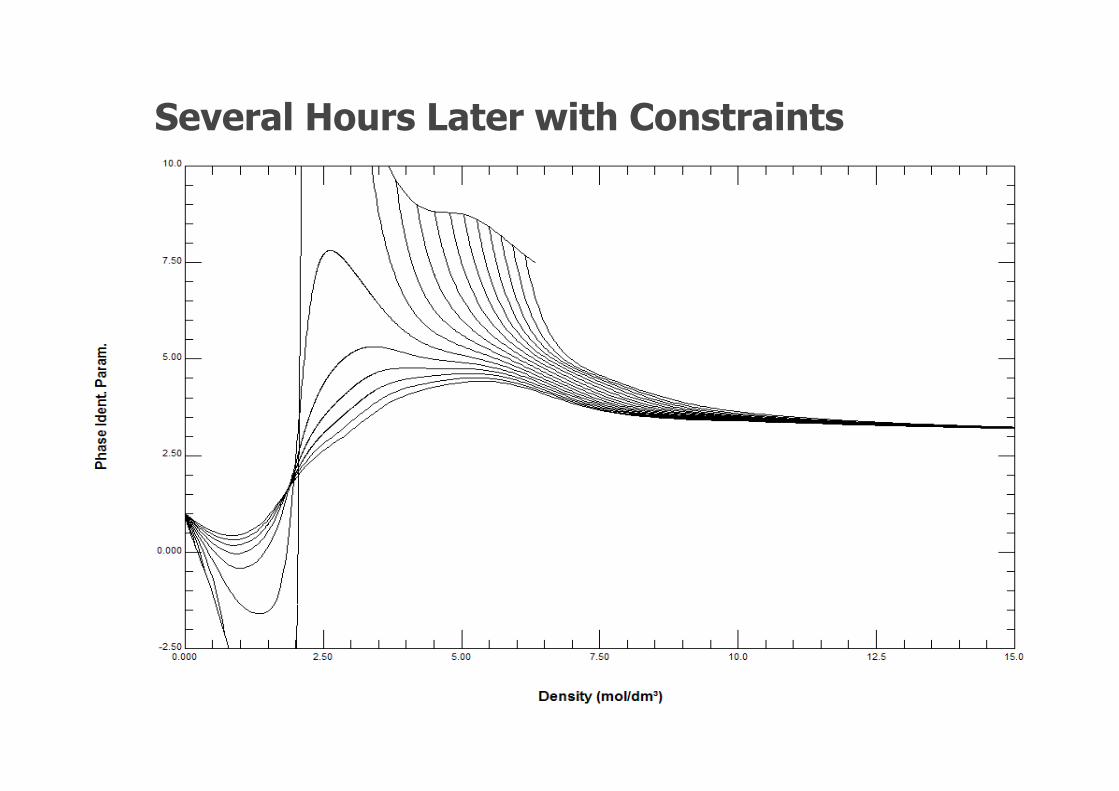
Several Hours Later with Constraints

Preliminary Helium Equation
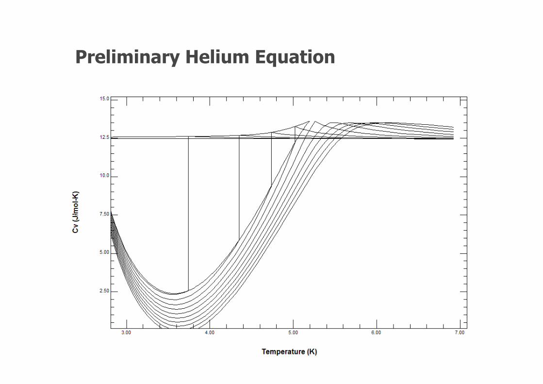
Preliminary Helium Equation

Methanol

Red arrows represent a partial derivative with respect to temperature.
Blue arrows represent a partial derivative with respect to density.
Thermodynamic Tree
Real Tree

Virial expansion◦ Gas phase only
Extended corresponding states◦ Slow and sometimes nonconvergent◦ Has the ability for high accuracy
Coefficient mixing of multiparameter equations◦ Requires fixed functional form for pure fluids
Excess Helmholtz energy with and T ◦ High accuracy with high convergence
Mixture Equations of State

Mixture Equations of State
Natural gas equations of state◦ SGERG-88 and AGA-8: Volumetric properties only Gas phase only No dew points
New reference equation of state◦ GERG-2008: Volumetric and caloric properties Fundamental equation of state Valid for all fluid or gas states Bubble and dew point calculations

0
100
200
300
-183 -150 -100 -50 0 50 77-3
liquid gas
critical point
phaseenvelope
AGA8-DC92
AGA8-DC92SGERG-88 0.1- 0.2 %w 0.2 %
Temperature
Pressure
1500
3000
4300
bar psia
°C
°F-150-240 -60 120320
100
200
300
-183 -150 -100 -50 0 50 77-3
liquid gas
critical point
phaseenvelope
AGA-8
SGERG-88 0.1 - 0.2 %w 0.2 %
Ranges of Application
GERG-2008
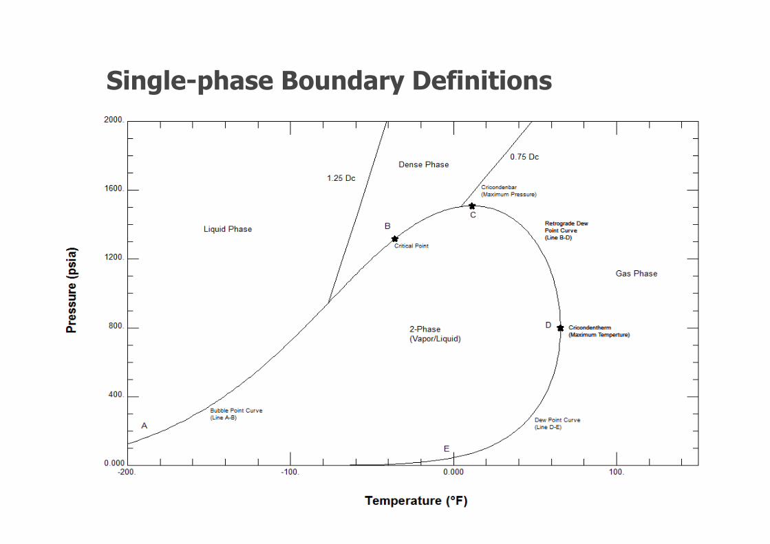
Single-phase Boundary Definitions
),(1
ideal
N
iiix
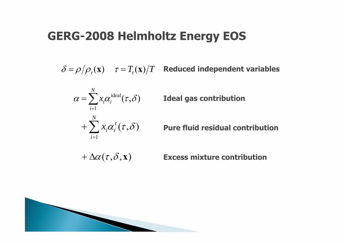
GERG-2008 Helmholtz Energy EOS
TT )( )( rr xx
Pure fluid residual contribution
Excess mixture contribution
Reduced independent variables
Ideal gas contribution
N
iiix
1
r ),(
),,( x
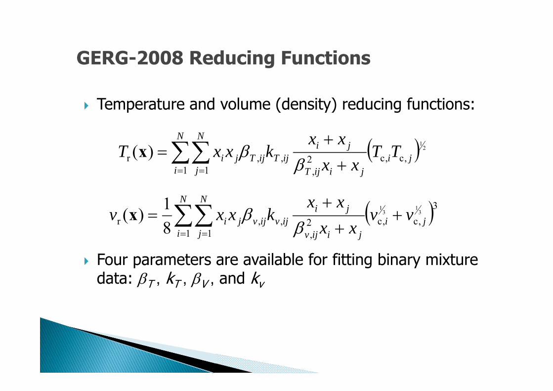
GERG-2008 Reducing Functions
21
,c,c1 1
2,
,,r )( ji
N
i
N
j jiijT
jiijTijTji TT
xxxx
kxxT
x
3,c,c1 1
2,
,,r3
13
1
81)( ji
N
i
N
j jiijv
jiijvijvji vv
xxxx
kxxv
x
Temperature and volume (density) reducing functions:
Four parameters are available for fitting binary mixture data: T , kT , V , and kv

When data are not available to fit interaction parameters, estimation schemes can be used.◦ Critical temperatures, critical pressures, and acentric factors can
be used to calculate the interaction parameter for the temperature reducing line:
mpq T
T 203.254.40crit2
crit1
Prediction Scheme
1
2crit
1
crit2
crit2
crit1
PP
TTm

Comparisons of Fitted and Predicted Values

Ph.D. Nitrogen 1973(original mBWR equation)
Jahangiri Ethylene 1986 Jahangiri Nitrogen 1986 Katti Neon 1986 Lemmon R11 1992 Penoncello R12 1992 Kamei R22 1995 Penoncello Cyclohexane 1995 Lemmon Air 2000 Leachman Hydrogen 2009 Lemmon Natural gas 1996
and refrigerant mixtures
Richard Jacobsen

Schmidt Oxygen 1985 Marx R11, R12 1992
R22, R113 Span CO2 1996 Tegeler Argon 1999 Span Nitrogen 2000 Smukala Ethylene 2000 Setzmann Methane 2000 Pruss Water 2002 Ethane Buecker 2006 Butanes Buecker 2006 Guder SF6 2009 Kunz GERG-2008
Wolfgang Wagner

Chair of mechanical engineeringin Bochum.
Developed equations of state for:◦ Ammonia Oxygen◦ Argon Pentane◦ Butane Propane◦ CO2 R-11◦ Cyclohexane R-113◦ Ethane R-12◦ Ethylene R-123◦ Heptane R-125◦ Heptane R-134a◦ Hexane R-143a◦ Isobutane R-152a◦ Methane R-22◦ Nitrogen R-32◦ Octane SF6
Developed a generalized correlation requiring only the critical point and acentric factor.
Has too many students to count.
Roland Span

Developed equations of state for:◦ Air Neopentane◦ Acetone Nitrous oxide◦ Butene Nonane◦ Carbon monoxide Propylcyclohexane◦ Carbonyl sulfide R-11◦ Cis-butene R-115◦ Cyclopentane R-116◦ Decane R-1233zd(E)◦ Dodecane R-1234yf◦ Hydrogen sulfide R-141b◦ Isobutene R-142b◦ Isohexane R-218◦ Isopentane R-227ea◦ Krypton R-365mfc◦ Methyl linoleate R-41◦ Methyl linolenate Sulfur dioxide◦ Methyl oleate Toluene◦ Methyl palmitate Trans-butene◦ Methyl stearate Trifluoroiodomethane◦ Methylcyclohexane Xenon
Mixture models for natural gas, refrigerants,and cryogens.
Refprop
Me

R‐143a1999
R‐232000
R‐1252002
Propylene2010
Propane2007
Ammonia2016
Ethane2020?
P-
Nonlinear Fitting Timeline

Satocis-Decalin
Span
Kortmann Amines
Schroeder (Idaho)Ethanol
Propylene
Ethane
R-125
Ammonia
Propane
R-23R-143a
Akasaka (Japan)R-1234ze(Z), R-32
R-1243zf, R-1336mzz
Leachman (Idaho)
Hydrogen
Herrig Heavy water
Blackham (Washington)
Isooctane
Ortiz-Vega (Texas)Helium
Richardson (Washington)
DeuteriumRomeo (Italy)
C16, C22
KunickHydrazine
Methylhydrazine
Wiens Ethanol/WaterOil Mixtures
Koester C4F10, C5F12,
C6F14
Gao (China)Ammonia1-Propanol
SO2Miyamoto (Japan)
Isopentane
Tietz Nitrogen tetroxide
Cristancho (Texas)
Propylene glycol
Alexandrov (Russia)Undecane
Generalized alkane modelOil fractions
Zhou
Ruan (China)MTBE
Pan (China)1-HexanolR-236fa
Bell (NIST)Ammonia/Water
Thol
GernertHumid air
Combustion Gases
The Student Explosion!
MatsumotoMethylcyclohexane

REFPROP - History

Select a pure fluid
TS diagrams
Phase Boundaries
PH diagrams
Choose Predefined mixtures
Select properties
Calculate tables of
properties
REFPROP – What does it look like?

REFPROP – Is It Actually Used? Nuclear Engineering◦ Recently cited by Jeong et al. in Nuclear
Engineering and Design where REFPROP was used for CO2 properties to design a sodium fast-cooled reactor with a supercritical CO2 Brayton cycle.
Design of working fluids for solar organic Rankine cycles ◦ Rayegan and Tao in Renewable Energy used
REFPROP to explore efficiency with different fluids.
Modeling the volatiles in volcanic eruptions ◦ Researchers at the University of Vancouver used
REFPROP to model the volatiles of a volcanic eruption as a mixture of CO2 and water.

REFPROP – Is It Actually Used? NASA◦ Nitrogen calculations to investigate the cause of
the Columbia space craft accident. ◦ Europa clipper mission.◦ Cryogenic systems for Mars missions.
SpaceX◦ Fuels (for example, methane and liquid oxygen)
and system components design. Aircraft and turbine design CERN◦ Attaining cryogenic conditions of the magnets.
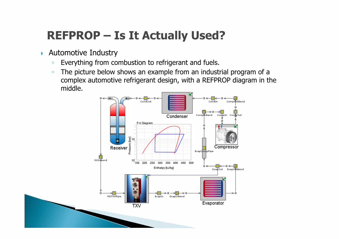
REFPROP – Is It Actually Used? Automotive Industry◦ Everything from combustion to refrigerant and fuels.◦ The picture below shows an example from an industrial program of a
complex automotive refrigerant design, with a REFPROP diagram in the middle.
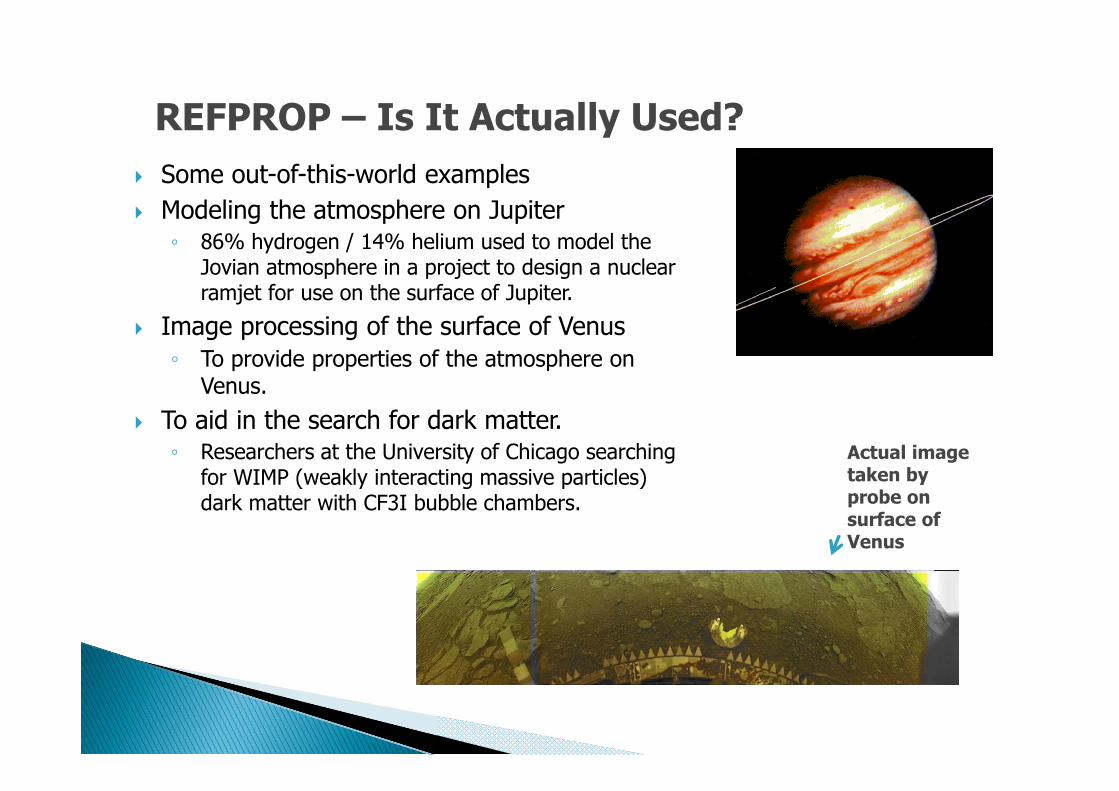
Actual image taken by probe on surface of Venus
REFPROP – Is It Actually Used? Some out-of-this-world examples Modeling the atmosphere on Jupiter
◦ 86% hydrogen / 14% helium used to model the Jovian atmosphere in a project to design a nuclear ramjet for use on the surface of Jupiter.
Image processing of the surface of Venus◦ To provide properties of the atmosphere on
Venus. To aid in the search for dark matter.
◦ Researchers at the University of Chicago searching for WIMP (weakly interacting massive particles) dark matter with CF3I bubble chambers.
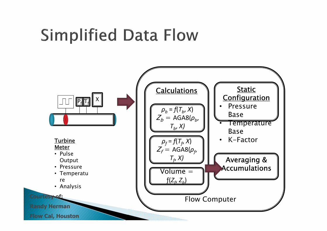
Flow Computer
Calculations
ρb = ƒ(Tb, X)Zb = AGA8(ρb,
Tb, X)
ρf = ƒ(Tf, X)Zf = AGA8(ρf,
Tf, X)
Volume = ƒ(Zf, Zb)
Averaging & Accumulations
Pf TfX
Turbine Meter• Pulse
Output• Pressure• Temperatu
re• Analysis
Static Configuration• Pressure
Base• Temperature
Base• K-Factor
Courtesy of:Randy HermanFlow Cal, Houston