ERDC/CRREL TR-14-6 'Runoff characterization and variations ... · 10 Discharge rating curve from all manual measurement for seasons 2009 –10 and 2010–11, generating equation (8)

ERD

C/CR

REL

TR-1

4-6

Engineering for Polar Operations, Logistics and Research (EPOLAR)

Runoff Characterization and Variations at McMurdo Station, Antarctica

Cold

Reg

ions

Res

earc

h an

d En

gine

erin

g La

bora

tory

Rosa T. Affleck, Meredith Carr, Margaret Knuth, Laura Elliot, Corey Chan, and Michael Diamond

May 2014

Early Austral Summer Middle of Austral Summer

Approved for public release; distribution is unlimited.

The US Army Engineer Research and Development Center (ERDC) solves the nation’s toughest engineering and environmental challenges. ERDC develops innovative solutions in civil and military engineering, geospatial sciences, water resources, and environmental sciences for the Army, the Department of Defense, civilian agencies, and our nation’s public good. Find out more at www.erdc.usace.army.mil.

To search for other technical reports published by ERDC, visit the ERDC online library at http://acwc.sdp.sirsi.net/client/default.

Engineering for Polar Operations, Logistics and Research (EPOLAR)

ERDC/CRREL TR-14-6 May 2014


Rosa T. Affleck and Meredith Carr Cold Regions Research and Engineering Laboratory (CRREL) US Army Engineer Research and Development Center 72 Lyme Road Hanover, NH 03755-1290

Margaret Knuth National Science Foundation Division of Polar Programs, Antarctic Infrastructure and Logistics 4201 Wilson Boulevard Arlington, VA 22230

Laura Elliot and Corey Chan Antarctic Support Contract 7400 S. Tucson Way Centennial, CO 08112

Michael Diamond University of Vermont Burlington, VT 05401

Final Report

Approved for public release; distribution is unlimited.

Prepared for National Science Foundation, Division of Polar Programs, Antarctic Infrastructure and Logistics Arlington, VA 22230

Under Engineering for Polar Operations, Logistics and Research (EPOLAR) EP-ANT 11-04, “McMurdo Drainage & Erosion Study: 2010–2011 Season”

ERDC/CRREL TR-14-6 iv

Abstract

As the austral summer approaches, major flow arteries are manually cleared in anticipation of the ephemeral runoff during the summer months. This flow, primarily from snowmelt, has daily and seasonal fluc-tuations. The flow fluctuation and variation depend on the air temperature and on many other factors. In addition, the runoff mobilizes sediment and localized soil contaminants that wash through these channels and dis-charge primarily into Winter Quarters Bay.

This report quantifies the runoff characteristics, including discharge corre-lations and variations for McMurdo Station drainage channels, and expands our understanding on the runoff charactestics at McMurdo Station. The flow data taken during austral summer 2010–11 combined with 2009–10 data fills the gaps in the analysis to quantify the runoff. Based on the correlation between the change in accumulated thawing de-gree days and cloudiness expressed in clearness, the time delay in the peak discharge can occur between 4 and 14 days after a peak temperature. Based on the frequency and probability distribution of the flow, a flow greater than 0.33 m3/s in the major channel occurred less than 5% of the time during the season. This study provides critical information for planning, operation and maintenance, the design of preventive methods, and the application of best practices.

DISCLAIMER: The contents of this report are not to be used for advertising, publication, or promotional purposes. Citation of trade names does not constitute an official endorsement or approval of the use of such commercial products. All product names and trademarks cited are the property of their respective owners. The findings of this report are not to be construed as an official Department of the Army position unless so designated by other authorized documents. DESTROY THIS REPORT WHEN NO LONGER NEEDED. DO NOT RETURN IT TO THE ORIGINATOR.

ERDC/CRREL TR-14-6 v

Contents Abstract .......................................................................................................................................................... iv

Illustrations .................................................................................................................................................... vi

Preface ...........................................................................................................................................................vii

Acronyms and Abbreviations ..................................................................................................................... ix

1 Introduction ............................................................................................................................................ 1

2 Background ............................................................................................................................................ 3

3 Methods .................................................................................................................................................. 9 3.1 Flow measurements ....................................................................................................... 9 3.2 Discharge rating curve and continuous discharge analyses ...................................... 10

4 Results ..................................................................................................................................................12 4.1 Flow depth versus discharge........................................................................................ 12 4.2 Continuous flow ............................................................................................................ 14 4.3 Flow frequency .............................................................................................................. 16 4.4 Timing of discharge ...................................................................................................... 20

5 Summary and Conclusions ............................................................................................................... 26

6 Recommendations .............................................................................................................................. 28

References ................................................................................................................................................... 29

Appendix A: Procedures for Flow Measurement and for Installation of Flow Sensors, 2010–11 Study .................................................................................................................................... 30

Appendix B: Flow Data Processing and Analysis ................................................................................. 35

Report Documentation Page

ERDC/CRREL TR-14-6 vi

Illustrations

Figures

1 Map of McMurdo Station showing the watershed boundary (dashed line) and the ice field contributing to the snowmelt. The watershed covers an area of approximately 5 km2 ...................................................................................................................... 2

2 Daily average air temperature at McMurdo Station for austral summers of 2009–10 and 2010–11 ............................................................................................................... 4

3. Daily maximum summer air temperatures at McMurdo for several years of record ................. 4 4 Net accumulated thawing degree days over several summers at McMurdo ......................... 5 5 McMurdo Station watershed and sub-basin boundaries ......................................................... 6 6 An example of an extreme incident showing raging water from snowmelt that

occurred on 12 December 2007 ................................................................................................. 7 7 Side berm emplaced as a temporary solution to contain the runoff during an

extreme event, 19 December 2010 ............................................................................................ 7 8 Typical cross-sections of major channels .................................................................................. 10 9 Discharge rating curve from manual measurement for seasons 2009–10 and

2010–11 for various locations ................................................................................................... 13 10 Discharge rating curve from all manual measurement for seasons 2009–10 and

2010–11, generating equation (8) (Table 2) ............................................................................ 14 11 Flow (QHOBO) recorded at station S1, S2B, S2C, and S3A for season 2010–11 .................. 15 12 Flow distribution for the austral summer of 2010–11 (note the difference in x-

scales on each plot) ..................................................................................................................... 18 13 Flow probability distribution for the austral summer of 2010–11 ........................................ 19 14 Lag time between air temperature and flow for drainage channel S2B, austral

summer 2010–11 ........................................................................................................................ 21 15 Lag time between air temperature and flow for drainage channel S2B, austral

summer 2009–10 ....................................................................................................................... 22 16 Lag time between peak temperature and flow related to Δmax ATDDnet with the

95% confident limits based on 1.96 times the standard error of the regression ............... 24 17 Lag time between air temperature and flow for drainage channel S2B, austral

summer 2007–08 ....................................................................................................................... 24

Tables

1 Sampling locations and descriptions ......................................................................................... 10 2 Discharge rating curves by location ........................................................................................... 13 3 Summary of statistical analysis during 2010–11 measurements ........................................ 16 4 Summary of warming events and their characteristics, 2009–11 ....................................... 21 5 Summary of likely warming events and their characteristics, austral summer

2007–08 ....................................................................................................................................... 25

ERDC/CRREL TR-14-6 vii

Preface

Funding for this effort was provided by the National Science Foundation, Division of Polar Programs, Antarctic Infrastructure and Logistics Section and the Office of Polar Environment, Safety and Health under Engineering for Polar Operations, Logistics and Research (EPOLAR) EP-ANT-11-04, “McMurdo Drainage & Erosion Study: 2010–11 Season.”

This report was prepared by Rosa Affleck (Force Projection and Sustain-ment Branch, Dr. Edel Cortez, Chief) and Dr. Meredith Carr (Remote Sensing/GIS and Water Resources Branch, Timothy Pangburn, Chief), US Army Engineer Research and Development Center (ERDC), Cold Regions Research and Engineering Laboratory (CRREL), Hanover, NH; Margaret Knuth, National Science Foundation, Division of Polar Programs, Antarc-tic Infrastructure and Logistics; Laura Elliot and Corey Chan, Antarctic Support Contract; and Michael Diamond, University of Vermont.

At the time of publication, Janet Hardy was the program manager for EPOLAR Antarctica; Dr. Justin Berman was Chief of the Research and En-gineering Division. The Deputy Director of ERDC-CRREL was Dr. Lance Hansen, and the Director was Dr. Robert Davis.

The 2010–11 field season study would not have been possible without as-sistance from Antarctic Support Contract staff: Marty Reed, John Horgan, and Ed Gawrys of Fleet Operations and Jeff Scanniello and Joe Massone for providing additional topographic data. In addition, the authors are grateful for the assistance provided by shipping, receiving, supply, and lo-gistics support at McMurdo Station during the field work.

Weather and other meteorological data used in this report were provided by the Antarctic Meteorological Research Center (http://amrc.ssec.wisc.edu/) through the supervision of Dr. Matthew Lazara. Existing geospatial data were provided by the Polar Geospatial Center (PGC) (http://www.pgc.umn.edu).

The authors also thank the following CRREL staff for their contributions: Kerry Claffey, who programmed the data collection for soil and tempera-ture probes; Callan George and Amy Burzynski (students) who compiled relevant data for analysis; Lynette Barna who provided assistance during

ERDC/CRREL TR-14-6 viii

the field work; and Renee Melendy for superb office administrative and logistical support. Most of all, the authors are grateful for the support from Joni Quimby for shipping and receiving the equipment and supplies used during the field work.

Emily Moynihan provided our editing support. Technical reviews were provided by former CRREL engineers Dr. Jon Zufelt (HDR Alaska, Inc.) and George Blaisdell (National Science Foundation, Division of Polar Pro-grams, Antarctic Infrastructure and Logistics).

The Commander of ERDC is COL Jeffrey R. Eckstein, and the Director of ERDC is Dr. Jeffery P. Holland.

ERDC/CRREL TR-14-6 ix

Acronyms and Abbreviations

ASCE American Society of Civil Engineers

ATDD Accumulated Thawing Degree Days

CRREL US Army Cold Regions Research and Engineering Laboratory

EPOLAR Engineering for Polar Operations, Logistics and Research

ERDC US Army Engineer Research and Development Center

PGC Polar Geospatial Center

RPSC Raytheon Polar Services Company

WQB Winter Quarters Bay

ERDC/CRREL TR-14-6 x

ERDC/CRREL TR-14-6 1

1 Introduction

McMurdo Station is a research facility and the logistics hub of the United States Antarctic Program, located on an outcrop of barren volcanic rock on the southern tip of Ross Island, Antarctica. From its establishment in the mid-1950s, the station slowly expanded in the 1960s; and rapid develop-ment continued over the following decades. Klein et al. (2008) recently documented a thorough historical background of the station’s develop-ment. Over this time, operational activities at the station have created some landscape changes and environmental disturbances (Klein et al. 2008; Klein et al. 2012; Kennicutt et al. 2010).

Through its evolution, McMurdo has had many infrastructure changes, including new facilities (buildings, cargo pads, etc.) and road network modifications. The expansion incorporated very limited geotechnical con-siderations during the changes. These changes also highlighted the drain-age challenges at the Station during periods of heavy flow of snowmelt runoff in the summer months, having created flow paths under and around buildings and across roads and parking lots. In addition, acci-dental spills and chemical contamination from leaking fuel and materials (lubricants, paints, etc.) brought to and used at the station have caused environmental alterations. Furthermore, the contaminants may have a tendency to be transported in the runoff during the snowmelt period.

The McMurdo watershed is bounded by high ridges and sloping hills of barren volcanic rock, extending up to perennial snow and ice fields and down to McMurdo Bay (Figure 1). Runoff from the watershed is mostly from snowmelt as liquid precipitation is rare at McMurdo.

The US Army Cold Regions Research and Engineering Laboratory (CRREL) conducted a preliminary drainage analysis and performed runoff measurements in the 2009-10 austral summer to characterize the amount of discharge from the watershed (Affleck et al. 2012a). To further quantify the runoff and its impacts on the station and on the local marine environ-ment, a second year of data collection was needed to capture the discharge variation. This phase of the study provided a second flow profile and aug-mented the pollutant analysis. Measurements included gathering manual and continuous flow information and collecting water samples at various


times and locations. The samples were sent off-site to a laboratory where they were analyzed for pollutant concentration. For a discussion of the re-sults, see Affleck et al. (forthcoming).

Figure 1. Map of McMurdo Station showing the watershed boundary (dashed line) and the ice field contributing to the snowmelt. The watershed covers an area of

approximately 5 km2 (Affleck et al. 2012a).

The objective of this report is to further characterize the snowmelt runoff, including discharge correlations and variations, for McMurdo Station drainage channels for two austral summers (2009–10 and 2010–11).


2 Background

Runoff in summer is driven primarily by the melting of snow and glacier ice (Affleck et al. 2012a, 2012b) and will be referred to in this paper simply as snowmelt runoff. The major flow paths at McMurdo Station are typical-ly filled with snow and ice in the winter months. As the austral summer approaches, major flow arteries are manually cleared in anticipation of the ephemeral runoff during these summer months. Snowmelt runoff passes through McMurdo via a system of drainage ditches, gullies, and culverts. The major flow paths are well-defined, earthen ditches that cross under the existing roads via culverts (Affleck et al. 2012a). Most of these drainage channels have very steep sides or embankment slopes and steep in-channel gradients. Most of the snowmelt runoff discharges into Winter Quarters Bay (WQB) and McMurdo Sound at several points.

The climate at McMurdo Station resembles a desert environment where, according to the daily meteorological data, the area receives very little pre-cipitation, which is mostly snow. Based on historical climate data, the daily maximum temperature for McMurdo Station (1 January 1973 to 13 March 2008) revealed that above-freezing temperatures normally occurred some-time between mid- to late November and late January or early February (Affleck et al. 2012a). The warming and cooling trends observed in this study during austral summers 2009–10 and 2010–11 reflect the historical climate data trends in temperature variations (Figure 2).

The daily air-temperature fluctuations at McMurdo depict several warm-ing events occurring during the summer months (Figure 2). During the austral summer of 2010–11, the first warm spell started the first week of November, with maximum temperatures rising above freezing on 10 No-vember (Figure 3). This first warm spell was followed with the tempera-ture dipping down to −10°C and a slight overall cooling trend through the end of November. At the beginning of December 2010, another warming event commenced; and, for the most part, the maximum air temperature stayed above freezing from 9 to 28 December. A return to a cooling trend began at the end of January 2011.


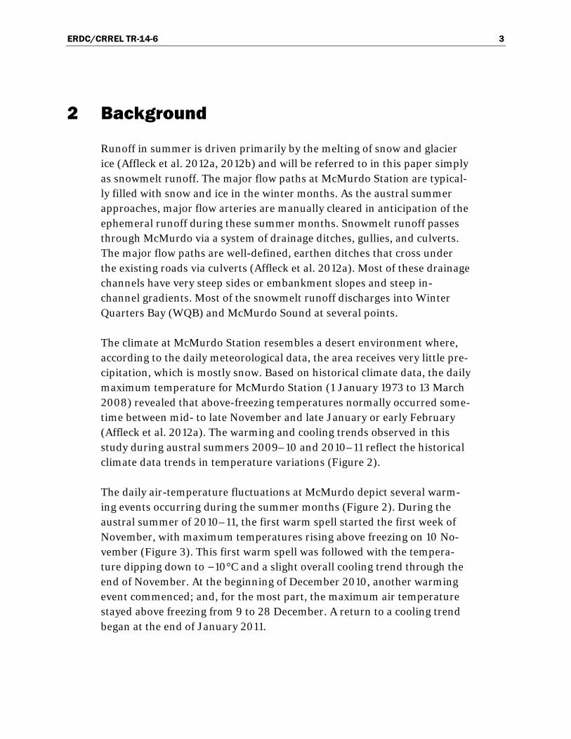
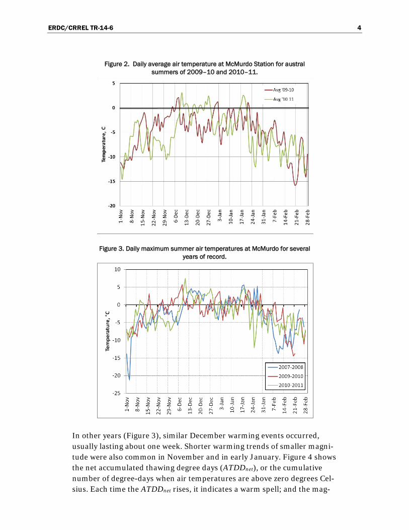
Figure 2. Daily average air temperature at McMurdo Station for austral summers of 2009–10 and 2010–11.

Figure 3. Daily maximum summer air temperatures at McMurdo for several years of record.

In other years (Figure 3), similar December warming events occurred, usually lasting about one week. Shorter warming trends of smaller magni-tude were also common in November and in early January. Figure 4 shows the net accumulated thawing degree days (ATDDnet), or the cumulative number of degree-days when air temperatures are above zero degrees Cel-sius. Each time the ATDDnet rises, it indicates a warm spell; and the mag-


nitude of the warm spell is indicated by the amplitude of the rise. The data shows that 2009–10 was a much cooler summer but that 2007–08 and 2010–11 were very similar with a strong warm spell in mid-December (about 15°C-days and 1.5 weeks long) and a shorter, smaller warm spell in mid-January (about 7°C-days and 3–4 days long).

Figure 4. Net accumulated thawing degree days over several summers at McMurdo.

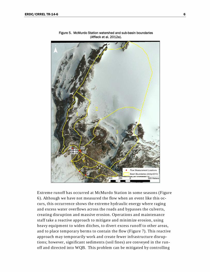
McMurdo Station watershed is one of the southernmost basins that annu-ally experiences active water flow (Figure 5). The watershed is divided into six basins. Three major sub-basins (1, 2, and 3) are located north of the Station and are largely covered with a perennial snow and glacial cover. The other three sub-basins (5, 6, and 7) are relatively small. Sub-basin 1 drains the area from the west along Hut Point Ridge and Arrival Heights, then along the road and down Hut Point Road. Sub-basin 2 has the largest area and encompasses the majority of the snowfield and the depression above Gasoline Alley. Sub-basin 3 includes the area north of the Main Road, then adjacent to Crater Hill, loops around portion of the snowfield, and continues on the east at the T-Site. Snowmelt runoff from sub-basins 2 and 3 merges downstream into WQB. Sub-basin 5 drains the area around the dorm, along the road towards the bay, and below the Water Treatment Plant. Sub-basin 6 is composed of the area south of the dorms and Main Road, along the road to the Chalet, and down to the road along the bay. Sub-basin 7 is the area south of the fuel tanks, around Observa-tion Hill, and below the Helo Pad.


Figure 5. McMurdo Station watershed and sub-basin boundaries (Affleck et al. 2012a).

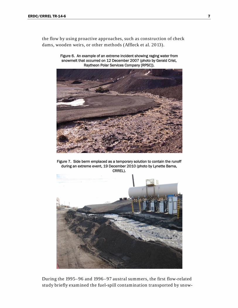
Extreme runoff has occurred at McMurdo Station in some seasons (Figure 6). Although we have not measured the flow when an event like this oc-curs, this occurrence shows the extreme hydraulic energy where raging and excess water overflows across the roads and bypasses the culverts, creating disruption and massive erosion. Operations and maintenance staff take a reactive approach to mitigate and minimize erosion, using heavy equipment to widen ditches, to divert excess runoff to other areas, and to place temporary berms to contain the flow (Figure 7). This reactive approach may temporarily work and create fewer infrastructure disrup-tions; however, significant sediments (soil fines) are conveyed in the run-off and directed into WQB. This problem can be mitigated by controlling

2 1

6

7

3

5


the flow by using proactive approaches, such as construction of check dams, wooden weirs, or other methods (Affleck et al. 2013).

Figure 6. An example of an extreme incident showing raging water from snowmelt that occurred on 12 December 2007 (photo by Gerald Crist,

Raytheon Polar Services Company [RPSC]).

Figure 7. Side berm emplaced as a temporary solution to contain the runoff during an extreme event, 19 December 2010 (photo by Lynette Barna,

CRREL).

During the 1995–96 and 1996–97 austral summers, the first flow-related study briefly examined the fuel-spill contamination transported by snow-


melt runoff in streams around McMurdo Station (Antarctic Support Asso-ciates 1995, 1997a, 1997b). Their studies indicated that runoff along the channels, including Gasoline Alley, by the Helo Pad, and along the main road (Figure 1), contained significant levels of fuel-related contamination that were picked up by the runoff along the channels (Figure 1). Recent studies by Kennicutt et al. (2010) and Klein et al. (2008, 2012) found that hydrocarbons in soils were high in areas where accidental spills occurred and in areas or pads where operational activities were taking place. They indicated that contamination in soils was contained in the areas where spills occurred and claimed that there had been limited redistribution of the contaminants. Affleck et al. (2012a) found that lateral flows from ice melting in the subsurface (i.e., active layer) occurred above and along the impermeable frozen soil layer. Thus, contaminants can potentially migrate into the permeable thawed ground and into the drainage channels during runoff.

A review of the runoff data collection and analysis and a comparison be-tween 2009–10 and 2010–11 flow results follow.


3 Methods

As this study is a continuation of the previous 2009–10 austral summer study (Affleck et al. 2012a), we used the same approach to monitor manual and continuous flow depths throughout the 2010–11 season. Appendix A highlights the details of the sampling strategy to monitor the runoff, and Appendix B describes procedures for flow data processing and analyses. This section summarizes the approaches used in the study.

3.1 Flow measurements

Manual flow data were measured at random times throughout the season and at defined locations listed in Table 1 and Figure 5. The measurements included the following:

• Bulk velocity—The average water velocity was determined based on the time it took a floating object to travel a known distance. Then the aver-age was multiplied by 0.85 to obtain the bulk velocity (representing a depth-averaged velocity value) for each location.

• Channel cross-sectional dimensions—Water depths and widths were measured by using a tape at three marked locations. From the center of the ditch, the water depths were measured in 12 cm intervals. The cross-sectional area was calculated using a trapezoidal approach.

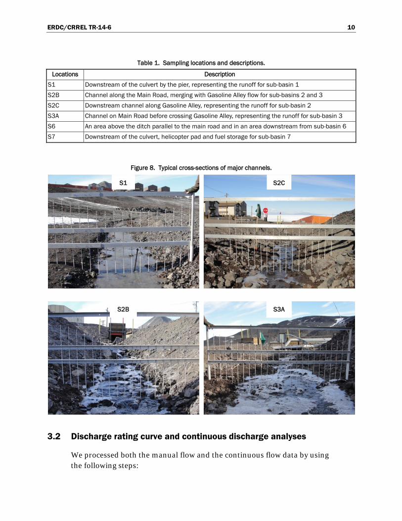
Figure 8 shows the typical profiles of the major channels. The S1 channel has a shallow trough shape. Both S2B and S2C channels have steep side slopes and typically have a narrow channel base. On the other hand, S3A tended to have a wide channel base with steep slope on one side.

Continuous flow depths were also measured at defined locations (Table 1; Figure 5) by using pressure transducer (capsule shape) sensors (i.e., HOBO water level logger). The pressure transducer sensors were pro-grammed to collect data every 15 minutes and were anchored on the bot-tom of the channels. We installed six sensors in the channels (i.e., S1, S2B, S2C, S3A, S6, and S7), and one was designated to measure the air pres-sure.


Table 1. Sampling locations and descriptions.

Locations Description S1 Downstream of the culvert by the pier, representing the runoff for sub-basin 1 S2B Channel along the Main Road, merging with Gasoline Alley flow for sub-basins 2 and 3 S2C Downstream channel along Gasoline Alley, representing the runoff for sub-basin 2 S3A Channel on Main Road before crossing Gasoline Alley, representing the runoff for sub-basin 3 S6 An area above the ditch parallel to the main road and in an area downstream from sub-basin 6 S7 Downstream of the culvert, helicopter pad and fuel storage for sub-basin 7

Figure 8. Typical cross-sections of major channels.

3.2 Discharge rating curve and continuous discharge analyses

We processed both the manual flow and the continuous flow data by using the following steps:

S1 S2C

S2B S3A


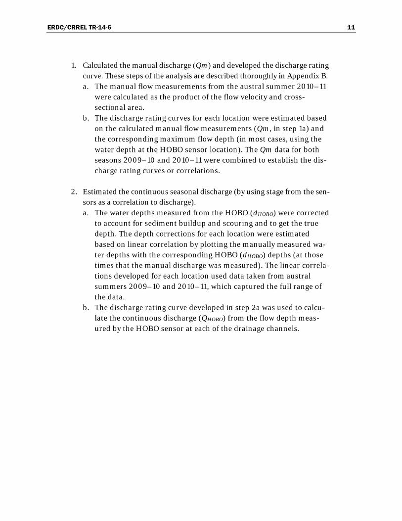
1. Calculated the manual discharge (Qm) and developed the discharge rating curve. These steps of the analysis are described thoroughly in Appendix B. a. The manual flow measurements from the austral summer 2010–11

were calculated as the product of the flow velocity and cross-sectional area.

b. The discharge rating curves for each location were estimated based on the calculated manual flow measurements (Qm, in step 1a) and the corresponding maximum flow depth (in most cases, using the water depth at the HOBO sensor location). The Qm data for both seasons 2009–10 and 2010–11 were combined to establish the dis-charge rating curves or correlations.

2. Estimated the continuous seasonal discharge (by using stage from the sen-sors as a correlation to discharge). a. The water depths measured from the HOBO (dHOBO) were corrected

to account for sediment buildup and scouring and to get the true depth. The depth corrections for each location were estimated based on linear correlation by plotting the manually measured wa-ter depths with the corresponding HOBO (dHOBO) depths (at those times that the manual discharge was measured). The linear correla-tions developed for each location used data taken from austral summers 2009–10 and 2010–11, which captured the full range of the data.

b. The discharge rating curve developed in step 2a was used to calcu-late the continuous discharge (QHOBO) from the flow depth meas-ured by the HOBO sensor at each of the drainage channels.


4 Results

The results here characterize the following: a discharge rating curve for each channel (Section 4.1), the continuous flow estimate for the entire aus-tral summer of 2010–11 (Section 4.2), the frequency and probability dis-tribution of the flow (Section 4.3), and the timing of peak discharge (Sec-tion 4.4).

4.1 Flow depth versus discharge

The individual discharge rating curve at each location produced a square-root equation as the best model fit. Table 2 summarizes the correlations and the parameter statistical errors. All of the correlations in Table 2 pro-duced statistical significance and resulted in probability of error values (p-value) of less than 0.001, indicating the significance in the interaction be-tween discharge and water depth. (The smaller the p-value, the more sig-nificant the correlation results.) The discharge rating curve, plotting the manual discharge measurement (Qm) versus the corresponding maximum flow depth (at time of measurement), was generated for each location (Figure 9). Manual flow measurements for the austral summer season 2010–11 seemed to complement data from season 2009–10, which filled in the gaps in the analysis. Also, each season reflected different amounts of discharge because snowmelt responds to air temperature and to solar gain; 2009–10 discharge was lower than the 2010–11 discharge data. The 95% statistical confidence intervals (the dashed lines in Figure 9) indicate the reliability of estimating discharge for particular flow depths. This assumes that flow data within the 95% confidence intervals is normally distributed at each depth.

Furthermore, combining all the datasets for all locations and for both sea-sons seemed logical because the data generated a correlation with an R square of 0.7560 (Figure 10) and the correlation produced equation (8) in Table 2. Equation (8) did not alter the estimated discharge, in contrast to using the individual equation at each location as listed in Table 2.


Table 2. Discharge rating curves by location.

Location Correlation Root Mean Square Error R Square Equation S1 𝑄 = 6.507𝑑2 0.0368 0.7616 (1) S2B 𝑄 = 4.631𝑑2 0.0280 0.9009 (2) S2C 𝑄 = 7.634𝑑2 0.0724 0.3111 (3) S3A 𝑄 = 6.366𝑑2 0.0332 0.7601 (4) S2B, S2C, and S3A 𝑄 = 5.413𝑑2 0.0199 0.7438 (5) S6 𝑄 = 3.166𝑑2 0.0157 0.7272 (6) S7 𝑄 = 4.783𝑑2 0.0088 0.9480 (7) All data together 𝑸 = 𝟓. 𝟑𝟖𝟐𝒅𝟐 0.0390 0.7560 (8) Where

Q is discharge (m3/s) d is maximum depth of water in the channel (m)

Figure 9. Discharge rating curve from manual measurement for seasons 2009–10 and

2010–11 for various locations.

(a) S1 (b) Combined data for these locations: S2B, S2C, and S3A

(c) S6 (d) S7


Figure 10. Discharge rating curve from all manual measurement for seasons 2009–10 and 2010–11,

generating equation (8) (Table 2).

4.2 Continuous flow

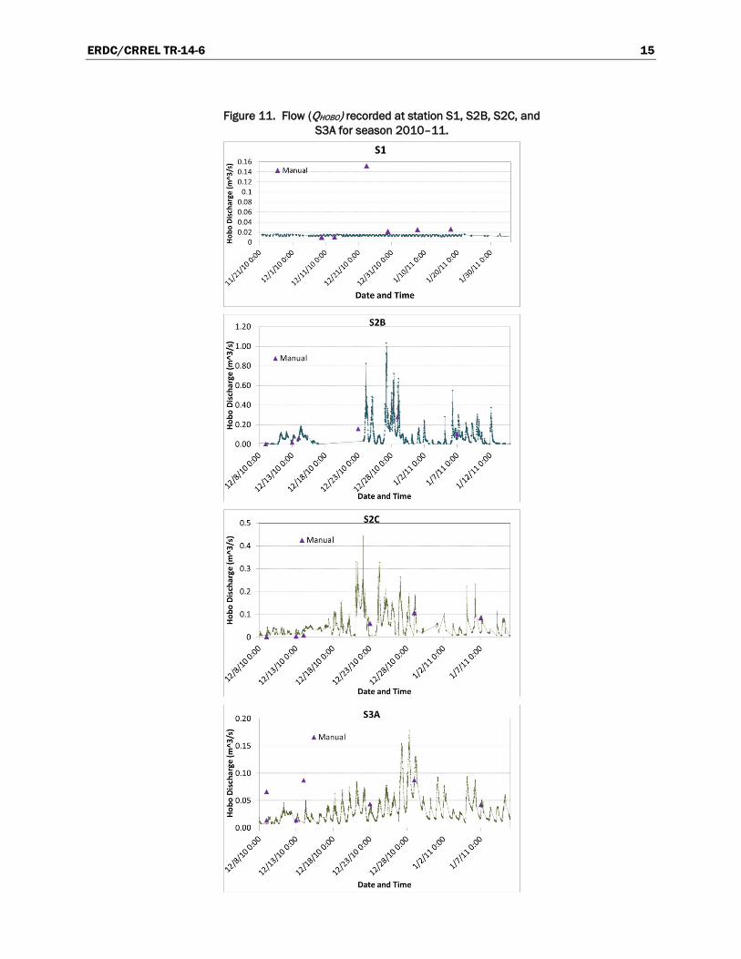
Equation (8) in Table 2 was used to estimate the continuous discharge, QHOBO. Appendix B shows the estimates for continuous flow measured us-ing pressure transducers (HOBO) in all six locations over the entire austral summer of 2010–11. The flow at S1, for most of the season, was 0.03 m3/s or below; and the flow stage (e.g., flow depth) showed that the sensor was mostly not submerged in the water. Although a Qm (manual Q) value of 0.15 m3/s was measured at S1, this particular Qm value could be an anom-aly or a measurement error (considering there was only one measurement showing this variation).

The critical channels at McMurdo Station with significant runoff are S2C and S3A, which merge into S2B. In general, the continuous flow rate in these critical channels depicted large diurnal variations (Figure 11). The data showed that runoff started on 11 December and then fluctuated and subsided for several days. These patterns continued with varying flow peaks throughout the season (Figure 11). On 19 December 2010, the max-imum flow rate at S2C (along Gasoline Alley) was approximately at 0.2 m3/s; this reflected the condition in Figure 7, requiring the emplacement of a control measure. However, the maximum flow rate at S2C of 0.44 m3/s occurred on 22 December 2010. Runoff from S2C and S3A merged to flow along S2B; the estimated maximum flow at S2B of 1.03 m3/s occurred on 27 December 2010.

0

0.0

0.1

0.1

0.2

0.2

0.3

Q (m

^3/s

)

0 0.05 0.1 0.15 0.2

Depth (m)


Figure 11. Flow (QHOBO) recorded at station S1, S2B, S2C, and S3A for season 2010–11.


4.3 Flow frequency

Although frequency analysis of a flow stage is normally done in big streams or rivers for multi-years data, a way to characterize the runoff at McMurdo Station is to quantify the seasonal flow statistics. Because the sensors collected data every 15 minutes, we can determine the flow distri-bution throughout the season from QHOBO data. Table 3 describes the flow distribution statistical summary from QHOBO at each location during aus-tral summer 2010–11, including estimated total volume at each channel. Approximately 39% of the total discharge (in volume) was transported at S2C while 32% of estimated volume was transported at S3A. These repre-sented an estimated total volume of 212,758 m3 discharged at S2B and contributed snowmelt runoff of 71% from sub-basins 2 and 3. The total volume of water discharge at S2B during the austral summer 2010–11 was significantly higher (compare to 30,875 m3, Affleck et al. 2012a) than the previous austral summer. The total discharge at S1 from sub-basin 1 only contributed roughly 18% and another 11% of flow came from S6 and S7 (sub-basins 6 and 7).

Table 3. Summary of statistical analysis during 2010–11 measurements. Austral Summer 2010–11

Location Days* Mean (µ) Q

(m3/s) Max. Q (m3/s) Min. Q (m3/s) Std. Dev.

(σ) Std. Error Mean (µ) Total Vol.† (m3)

S1 68 0.013 0.017 0.011 0.001 2.12e-5 54,939

S2B 57 0.103 1.033 0.002 0.117 0.002 212,758‡

S2C 44 0.058 0.443 0.007 0.054 0.001 116,550

S3A 53 0.032 0.178 0.006 0.025 4.3e-4 96,208

S6 57 0.004 0.005 0.002 — — 11,928

S7 57 0.008 0.033 — — — 20,561 * Number of monitoring days. † Estimated volume from continuous discharge (HOBO sensor) for the corresponding number of days. ‡ Combined volume from S2C and S3A. — Insignificant values.

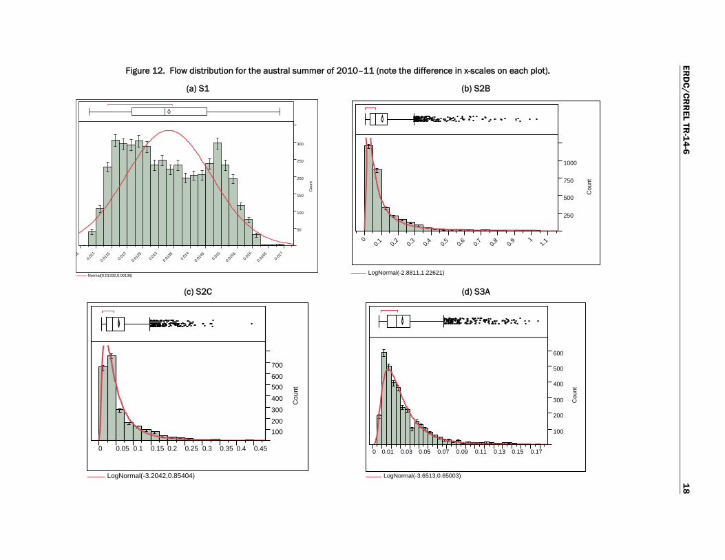
In addition, we can further quantify the flow characteristics by analyzing frequency and probability distributions of the flow, given the conditions for the season. The frequency distribution (histogram) counts the occur-rences of flow within the intervals (as shown in Figure 12). Typically in the frequency analysis, a curve-fit function (distribution function) is applied. The distribution of the data can produce various shapes, such as a normal or skewed shape distribution, which is a derivation of mean (µ) and vari-ance (σ2) (Natrella 1963). The frequency distribution function will then provide an estimate of probability


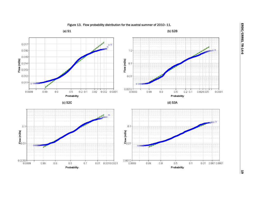
For this study, it is useful to ask what chance certain levels of discharge have of occurring. Figure 13 is the cumulative distribution function that represents the probability of a given discharge exceeding certain values during the austral summer of 2010–11. On this log probability scale, a probability of 0.1 means a 10% chance of equaling or exceeding the dis-charge value.

The flow at the S1 channel during austral summer 2010–11 exhibited a uniform distribution with average flow of 0.013 m3/s (Figure 12a). A flow of 0.0157 m3/s occurred less than 5% of the time, and a flow of 0.012 m3/s happened approximately 90% of the time during the season (Figure 13a). The flow at S1 showed no significant fluctuation throughout the season; a retention pond upstream to catch the snowmelt in the sub-basin attenuat-ed the flow.

The average flow at S2B was 0.103 m3/s, and the frequency distribution produced a skewed function with some high flows on the tail (right) side of the distribution (Figure 12b). The skewedness depicted the behavior of fluctuating flow throughout the season, and this distribution is represent-ed with a probability log-log function with respect to flow, Q (Figure 13b). A flow of less than 0.015 m3/s happened more than 90% of the time, and flow greater than 0.33 m3/s occurred less than 5% of the time during the season (Figure 13b). This meant that higher flows could occur given the ideal conditions for extreme runoff.

During the austral summer 2010–11, the flow at S2C channel, along Gaso-line Alley, exhibited a right skewed distribution with an average flow of 0.058 m3/s (Figure 12c). Similarly, a log function represented the proba-bility with respect to the distribution of flow (Figure 13c). A flow of 0.015 m3/s occurred 90% of the time and a flow of 0.136 m3/s happened 5% of the time during the season.

Similar to S2B and S2C, the flow frequency distribution at S3A produced a skewed function with some high flows on the right side of the distribution (Figure 12d) and gave a log-log function in the distribution of flow (Figure 13d). The average flow was approximately 0.032 m3/s. A flow level of 0.012 m3/s occurred 90% of the time, and a flow greater than 0.08 m3/s occurred less than 5% of the time during the season.

ERD

C/CRR

EL TR-14-6

18

Figure 12. Flow distribution for the austral summer of 2010–11 (note the difference in x-scales on each plot).

(a) S1 (b) S2B

(c) S2C (d) S3A

50

100

150

200

250

300

Cou

nt

050.0

11

0.011

50.0

12

0.012

50.0

13

0.013

50.0

14

0.014

50.0

15

0.015

50.0

16

0.016

50.0

17

Normal(0.01332,0.00136)

250

500

750

1000

Cou

nt

00.1 0.2 0.3 0.4 0.5 0.6 0.7 0.8 0.9

11.1

LogNormal(-2.8811,1.22621)

100200

300

400

500600

700

Cou

nt

0 0.05 0.1 0.15 0.2 0.25 0.3 0.35 0.4 0.45

LogNormal(-3.2042,0.85404)

100

200

300

400

500

600

Cou

nt

0 0.01 0.03 0.05 0.07 0.09 0.11 0.13 0.15 0.17

LogNormal(-3.6513,0.65003)

ERD

C/CRR

EL TR-14-6

19

Figure 13. Flow probability distribution for the austral summer of 2010–11.

(a) S1 (b) S2B

(c) S2C (d) S3A


4.4 Timing of discharge

As the temperature gradually rises, snow and ice accumulation in the drainage channels are manually cleared to accommodate the impending snowmelt runoff. Therefore, knowing when the runoff occurs is critical for operation and maintenance of the channels. There are other critical driv-ers that also influence the runoff, such as solar gain. We conducted an analysis of indicators relating the air temperature and cloud cover to flow rate to quantify when significant flow occurred. Indicators for air tempera-ture were used based on the date when peak maximum temperature oc-curred, the start date when the temperature was above freezing for greater than 3 consecutive days, and the corresponding maximum change (Δmax) in ATDDnet (in °C-days). The indicator for daily cloud cover is expressed in terms of clearness to represent the solar input. Clearness was evaluated as 100% minus the reported cloudiness (%). We used the maximum clearness over the first three days above freezing. Lag time is the indicator used to represent the time period between peak temperature and peak flow (in days).

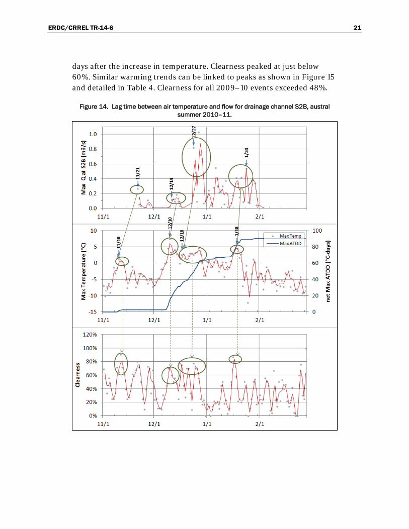
Early in the austral summer 2010–11 season, during the first warming trend, data indicated that the first major runoff occurred on 21 November and was the result of a warm period where the maximum temperature rose to near 0°C on 10 November (Figure 14). Another cycle of runoff on 27 November was likely caused by a warm period that occurred on 18 No-vember though this warm spell did not exceed freezing temperatures and clearness was low compared to other events. These factors indicated that this event may have been too small to identify with this analysis. Lower temperatures followed, which was reflected in the runoff dropping to al-most zero. Another warming trend occurred during the first week of De-cember when the maximum temperature hovered above zero for several days (peak at 6.8°C on 10 December), resulting in significant flow starting on 13 December and tapering off six days later (19 December). A consider-able runoff event occurred on 27 December following the 18 December high temperatures. At this point in time, runoff was likely to continue as there was enough ground surface energy to generate snow melting until the air temperature started to dive back below freezing continuously. All events except 28 November were preceded by a clearness of at least 70% in the first 3 days above freezing.

The previous austral summer, 2009–10, had frequent warm spells starting 25 November. The first peak in stage occurred on 9 December, about 14


days after the increase in temperature. Clearness peaked at just below 60%. Similar warming trends can be linked to peaks as shown in Figure 15 and detailed in Table 4. Clearness for all 2009–10 events exceeded 48%.

Figure 14. Lag time between air temperature and flow for drainage channel S2B, austral summer 2010–11.


Figure 15. Lag time between air temperature and flow for drainage channel S2B, austral summer 2009–10

0

20

40

60

80

100

-15

-10

-5

0

5

10

11/1 12/1 1/1 2/1

net M

ax A

TDD

(°C-

days

)

Max

Tem

pera

ture

(°C)

Max TempMax ATDD1/

2

12/1

912

/19

0%

20%

40%

60%

80%

100%

120%

11/1 12/1 1/1 2/1

Clea

rnes

s

0.00

0.02

0.04

0.06

0.08

0.10

0.12

11/1 12/1 1/1 2/1

Max

Q a

t S2B

(m3/

s)

11/2

5

1/23

12/9 12/1

7

12/2

7

1/11

12/8

1/11


Table 4. Summary of warming events and their characteristics, 2009–11.

Austral Summer

Date of Peak Temp

Date of Temp > 0°C for 3 days

Max Clearness over 3 days

Δmax ATDDnet (°C-days)

Date of peak Q

Magnitude of Peak Q (m3/s)

Δ peak temp to peak Q (days)

Δ Temp > 0°C for 3 days to peak Q (days)

2009–10 11/25 11/25 59% 1.8 12/9 0.138 14 14

12/8 12/5 62% 3.6 12/17 0.097 9 12

12/19 12/18 48% 3.6 12/27 0.053 8 9

1/2 1/1 70% 8.0 1/11 0.037 9 10

1/11 1/11 67% 4.5 1/23 0.081 12 12

2010–11 11/10 11/12 91% 2.5 11/21 0.266 11 9

11/18 -- 41% 0 11/27 0.114 9 --

12/10 12/10 72% 12.4 12/14 0.184 4 4

12/18 12/20 75% 6.9 12/27 1.030 9 7

1/18 1/17 87% 7.6 1/24 0.542 6 7

min 48% 1.8 4 4

max 91% 12.4 14 14

mean 70% 5.6 9 9

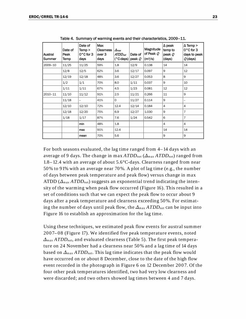
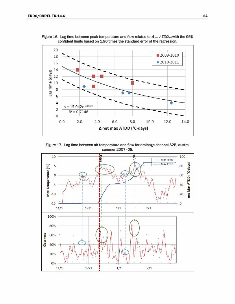
For both seasons evaluated, the lag time ranged from 4–14 days with an average of 9 days. The change in max ATDDnet (Δmax ATDDnet) ranged from 1.8–12.4 with an average of about 5.6°C-days. Clearness ranged from near 50% to 91% with an average near 70%. A plot of lag time (e.g., the number of days between peak temperature and peak flow) versus change in max ATDD (Δmax ATDDnet) suggests an exponential trend indicating the inten-sity of the warming when peak flow occurred (Figure 16). This resulted in a set of conditions such that we can expect the peak flow to occur about 9 days after a peak temperature and clearness exceeding 50%. For estimat-ing the number of days until peak flow, the Δmax ATDDnet can be input into Figure 16 to establish an approximation for the lag time.

Using these techniques, we estimated peak flow events for austral summer 2007–08 (Figure 17). We identified five peak temperature events, noted Δmax ATDDnet, and evaluated clearness (Table 5). The first peak tempera-ture on 24 November had a clearness near 50% and a lag time of 14 days based on Δmax ATDDnet. This lag time indicates that the peak flow would have occurred on or about 8 December, close to the date of the high flow event recorded in the photograph in Figure 6 on 12 December 2007. Of the four other peak temperatures identified, two had very low clearness and were discarded; and two others showed lag times between 4 and 7 days.


Figure 16. Lag time between peak temperature and flow related to Δmax ATDDnet with the 95% confident limits based on 1.96 times the standard error of the regression.

Figure 17. Lag time between air temperature and flow for drainage channel S2B, austral summer 2007–08.


Table 5. Summary of likely warming events and their characteristics, austral summer 2007–08.

Expected

Austral Summer

Date of Peak Temp

Date of Temp >

0°C for 3 days

Max Clearness

over 3 days

Δmax ATDDnet

(°C-days)

Δ Temp > 0°C for 3 days to

peak Q (days) Date of peak Q

2007–08 11/24 -- 45% 0.61 14.2 12/8 12/14 12/13 76% 8 7.0 12/20 1/8 1/6 23% 3.91 -- -- 1/10 1/12 39% 2.89 -- -- 1/18 1/18 62% 14 3.9 1/21

-- indicates that it probably did not occur due to low clearness or too short a cold spell.


5 Summary and Conclusions

This study characterized and quantified the runoff for McMurdo Station drainage. First, we developed a discharge curve rating for each channel by using the combined flow data taken during austral summer seasons 2010–11 and 2009–10, as described in Section 4.1. Second, we established an es-timate of the continuous flow along the major channels (S1, S2B, S2C, and S3A) for the entire austral summer of 2010–11 (Section 4.2). Third, we quantified the frequency and probability distribution of the flow to deter-mine the probability of occurrence of certain levels of discharge (Section 4.3). Lastly, we related the incidences when the runoff and peak flow oc-curred to the maximum temperature and cloud cover (Section 4.4). The overall summary included the following:

• Austral summers are characterized by brief warming trends of temper-atures above freezing and ATDDnet ranging from about 5°C-days to 25°C-days. The first warm spell could start during the first week of No-vember.

• High flow events are caused by snowmelt and can be extreme, causing extreme hydraulic energy where raging and excess water overflows roads and bypasses culverts, creating disruption and intensive erosion.

• Flow data were measured in 2009–10 and 2010–11 from manual measurements, and flow sensors provided us with discharge rating curves and continuous estimates of flow rates for snowmelt periods.

• A combined discharge rating curve for all sites was developed with a correlation coefficient, R2, of 0.7560.

• Significant runoff was recorded at S2C and S3A merging into S2B. Flow frequency analyses were conducted and showed average flows of 0.058 m3/s, 0.032 m3/s, and 0.103 m3/s, respectively. Average flows at S1, S6, and S7 were less than 0.015 m3/s.

• In the major channel (S2B), a flow of approximately 0.015 m3/s or less happened more than 90% of the time; and the occurrence of flow greater than 0.33 m3/s was less than 5% of the time during the season. However, there is a chance that higher flows could occur given ideal conditions, resulting in extreme runoff.

• Data show that discharge occurs 4–14 days after a peak temperature event and can be correlated with change in ATDDnet and a threshold maximum clearness.


• An estimated total volume of 212,758 m3 was transported at S2C and S3A during the austral summer 2010–11, totaling to 71% of contributed snowmelt runoff from sub-basins 2 and 3. Another 18% of discharge at S1 was contributed snowmelt runoff from sub-basin 1. All of which were discharged primarily into Winter Quarters Bay (WQB).

This study provided an expansion of our understanding of the runoff characteristics at McMurdo Station. The flow data taken during austral season 2010–11 combined with 2009–10 data filled the gaps in the analy-sis to quantify the runoff. The snowmelt runoff at McMurdo Station fluatuated in response to tempetature and solar input. Outcome from this study provides critical information for planning, operation and maintenance, design of preventive methods, and application of best practices.


6 Recommendations

Given the variability of the snowmelt runoff and extreme flow rates at McMurdo Station, one way to mitigate erosion is by implementing preven-tive approaches, such as best management practices or erosion control systems. These systems are often built to trap sediment and to control or attenuate flow in the receiving channels before the runoff exits into WQB at McMurdo Sound. Some channels have steep side slopes and require ap-propriate design slopes or stabilization techniques.

We recommend the following to mitigate erosion:

• A new plan for runoff by finding a better route for drainage, eliminat-ing several existing flow paths, and merging flow into one primary drainage path.

• Controlling the flow with the installation of settling ponds, weirs, and check dams to slow down the flow.


References Affleck, R. T., C. Vuyovich, M. Knuth, and S. Daly. 2012a. Drainage Assessment and Flow

Monitoring at McMurdo Station during Austral Summer. ERDC/CRREL TR-12-3. Hanover, NH: US Army Research Engineering and Development Center.

Affleck, R., M. Knuth and S. Arcone. 2012b. Snow and Climatic Characterization Influencing Snowmelt at McMurdo Station. In Proceedings of the ASCE 15th International Specialty Conference on Cold Regions Engineering, 19-22 August 2012, Quebec City, Canada. Reston, VA: American Society of Civil Engineers.

Affleck, R., M. Carr, and B. West. 2013. Modeling and Designing Control Flow Systems for McMurdo Station Drainage Channels. In Proceedings of the ASCE 10th International Symposium on Cold Regions Development.

Affleck, R.T., M. Carr, L. Elliot, C. Chan and M. Knuth. Forthcoming. Pollutant Concentration in Runoff at McMurdo Station, Antarctica. ERDC/CRREL Technical Report. Hanover, NH: US Army Research Engineering and Development Center.

Antarctic Support Associates. 1995. 1994–1995 surficial soil sampling and analysis McMurdo Station, Antarctica. 17 April 1995.

Antarctic Support Associates. 1997a. Phase Two snowmelt runoff and associated sediment soil sampling and analysis McMurdo Station, Antarctica. April 1997.

Antarctic Support Associates. 1997b. Sampling and analysis report, phase three, snowmelt runoff and associated sediment, McMurdo Station, Antarctica. August 1997.

Kennicutt, M. C., II, A. Klein, P. Montagna, S. Sweet, T. Wade, T. Palmer, J. Sericano, and G. Denoux. 2010. Temporal and spatial patterns of anthropogenic disturbance at McMurdo Station, Antarctica. Environmental Research Letters. 5(3):034010.

Klein, A. G., S. T. Sweet, T. L. Wade, J. L. Sericano, and M. C. Kennicutt II. 2012. Spatial patterns of total petroleum hydrocarbons in the terrestrial environment at McMurdo Station, Antarctica. Antarctic Science 24(5):450–466.

Klein, A, M. Kennicutt, G. Wolff, S. Sweet, T. Bloxom, D. Gielstra, and M. Cleckley. 2008. The historical development of McMurdo station, Antarctica, an environmental perspective. Polar Geography 31:119-144.

Natrella M. G. 1963. Experimental Statistics, Handbook 91. United States Department of Commerce, National Bureau of Standards.


Appendix A: Procedures for Flow Measurement and for Installation of Flow Sensors, 2010–11 Study

RPSC Environmental staff assisted CRREL in the development and im-plementation of the runoff sampling. The following highlights the steps for implementation.

HOBO sensors installation

We took the following steps to install the pressure transducers (HOBO):

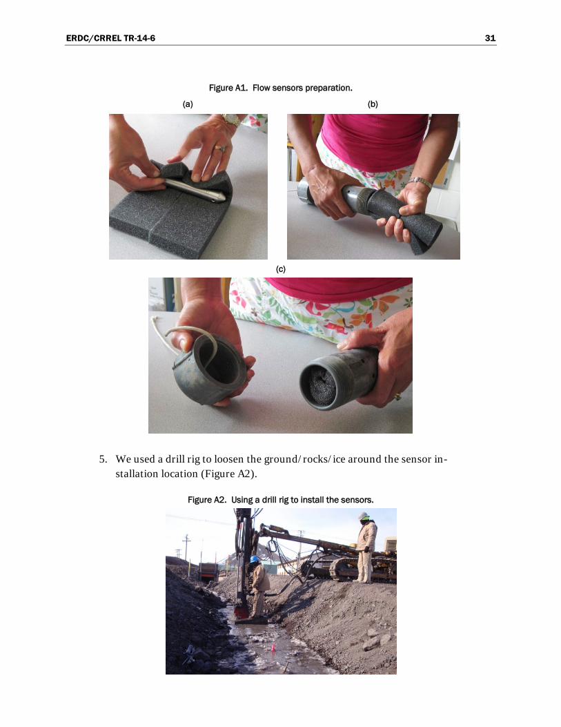
1. We programmed the HOBO to start collecting data on 21 November 2010 at 1200 hours; then we wrapped each of the HOBO with sheets of foam (Figure A1a) to make sure each of them was fully covered.

2. We placed each HOBO into a PVC casing (Figure A1b). 3. We tightly wrapped the plastic end caps with a layer of Teflon tape around

the threads of the PVC case Figure A1c. We marked each sensor to be de-ployed at a particular location according to Table A1.

4. Once we had prepared the sensors inside the protective casing, we in-stalled the sensors securely in the ditches. (This required Fleet Operations support and coordination to drill the anchors.)

Table A1. Location coordinates.

HOBO LAT (South) LONG (East) Comments S1 −77.84397144 166.6564921 Downstream of the culvert S2B-DS −77.84440319 166.6639117 First HOBO for location S2B, just few feet

from S2B-US (DS means downstream) S2B-US −77.84441637 166.6639839 2nd HOBO for location S2B, just few feet

upstream of S2B-DS S2C −77.84436458 166.6649383 S3A −77.84468681 166.6655503 S6 −77.84917101 166.6648414 S7 −77.84141098 166.671281 Coordinates of the culvert outlet over by

the Helo Pad place this HOBO downstream of culvert


Figure A1. Flow sensors preparation.

(a) (b)

(c)

5. We used a drill rig to loosen the ground/rocks/ice around the sensor in-stallation location (Figure A2).

Figure A2. Using a drill rig to install the sensors.


6. We attached metal braces to each casing and away from the holes in the PVC as shown in Figure A3.

Figure A3. Fasteners used to install the sensors.

7. We used long nails/stakes to center the sensor in the ditch as best as pos-sible (Figure A4a).

8. We installed stake upstream and downstream of the sensor by drilling a hole in the ground and attached strings on the casing to the stakes to se-cure the sensor further (Figure A4b).

Figure A4. Anchoring the sensors.

9. We noted the date and time when each sensor was placed into the water. 10. We marked the location on the side of the ditch with wooden poles approx-

imately 2.5 m (8.25 ft) upstream and downstream of the sensor or used the upstream and downstream backup stakes for markers, and used these markers for the manual flow measurements, as described below.

a. b.


11. We installed one HOBO in the air (Figure A5), hung in a safe location out-side and protected from the wind. We noted the date and time that we in-stalled this HOBO was installed.

Figure A5. Atmospheric measurement sensor.

Manual flow measurements

We took manual measurements when possible to validate the HOBO sen-sor data, recording in a field book the date and time for every measure-ment taken. The steps we used to collect manual flow measurements fol-low:

1. Using the markers (as transect), we measured the widths of the ditch at the top, center (on the upstream side of HOBO sensor), and bottom locations (Figure A6).

2. The cross-sectional depths were measured with the following: c. Using a bamboo pole and sharpie, we placed a mark at the center of

the bamboo stake as a zero line, then added 12 cm intervals mark-ings on each side of the zero mark.

d. Placing the bamboo pole perpendicular to the ditch and aligning the zero mark at the center of the ditch, we used a yard stick to measure the water depths at each (12 cm interval) marking on the bamboo pole. When measuring the water depth under fast current, we took the average value.


Figure A6. Transect measurement scheme.

3. Using the markers in step 10 above and while standing downstream of the last marker on the bottom transects, we tossed a ping-pong ball approxi-mately 0.5 m upstream of the top transect. We noted the time the ball took to float between the top and bottom transects and repeated this three times. We used this to calculate the water velocity and to validate data tak-en by the pressure transducers.

4. We recorded the water depths at the front, back and on each side (in the center) of the HOBO casing (see points a–d in Figure A6). This was be-cause over the course of time that the HOBO sensor was in the channel, sediments either would be built-up or scoured around the HOBO casing. These depths were necessary for correlating the HOBO depths described in Appendix B, HOBO Depth Corrections section.


Appendix B: Flow Data Processing and Analysis

Manual Flow

First, we derived an average water velocity from the three tests by using the ping-pong ball’s recorded time and distance traveled. We calculated the bulk velocity at each location by multiplying this average by 0.85. We calculated the area of the ditch by using a “trapezoidal” method. The trap-ezoidal method used 12 cm profiles of the ditch and calculated the area of the 12 cm section. Next, we calculated a discharge (also known as Qm) from the area and bulk velocity (Q = Velocity × Area).

Discharge rating curve for 2010–11 manual dataset

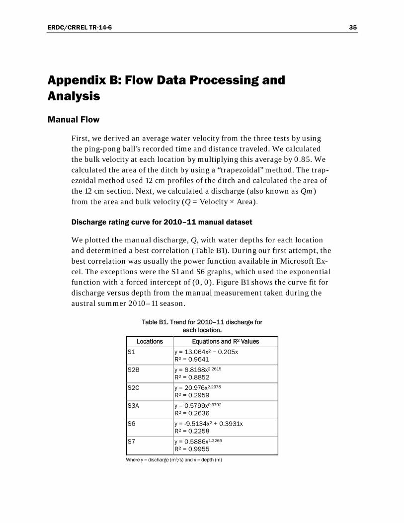
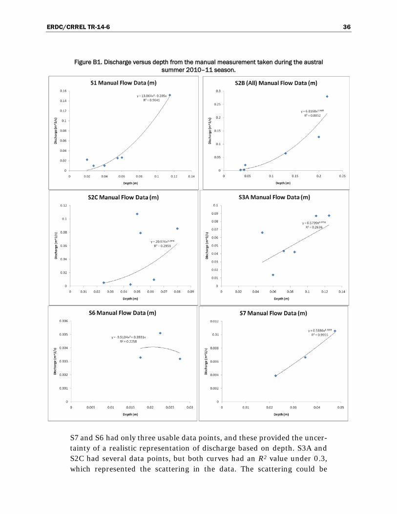
We plotted the manual discharge, Q, with water depths for each location and determined a best correlation (Table B1). During our first attempt, the best correlation was usually the power function available in Microsoft Ex-cel. The exceptions were the S1 and S6 graphs, which used the exponential function with a forced intercept of (0, 0). Figure B1 shows the curve fit for discharge versus depth from the manual measurement taken during the austral summer 2010–11 season.

Table B1. Trend for 2010–11 discharge for each location.

Locations Equations and R2 Values S1 y = 13.064x2 − 0.205x

R² = 0.9641 S2B y = 6.8168x2.2615

R² = 0.8852 S2C y = 20.976x2.2978

R² = 0.2959 S3A y = 0.5799x0.9792

R² = 0.2636 S6 y = -9.5134x2 + 0.3931x

R² = 0.2258 S7 y = 0.5886x1.3269

R² = 0.9955 Where y = discharge (m3/s) and x = depth (m)


Figure B1. Discharge versus depth from the manual measurement taken during the austral summer 2010–11 season.

S7 and S6 had only three usable data points, and these provided the uncer-tainty of a realistic representation of discharge based on depth. S3A and S2C had several data points, but both curves had an R2 value under 0.3, which represented the scattering in the data. The scattering could be


measurement errors because multiple individuals were taking the data or the ditch widened halfway through the season. The scattering was clearly outlined when looking at the S2B, S2C, and S3A combined graph (Figure B2) where the higher discharge points for S2C did not fall in line within the rest of the data. The S2B and S1 discharge graphs looked reasonable though the highest depth and highest discharge were clearly well out of reach of any of the other measurements.

Figure B2. S2B, S2C, and S3A Manual Flow Data

Discharge rating curve for combined 2009–10 and 2010–11 manual data

When processing the data, we noticed that some areas (like S6, for exam-ple) had a limited number of points. We decided to combine the austral summer 2010–11 data along with austral summer 2009–10. Figure B3 shows these “combined” plots.

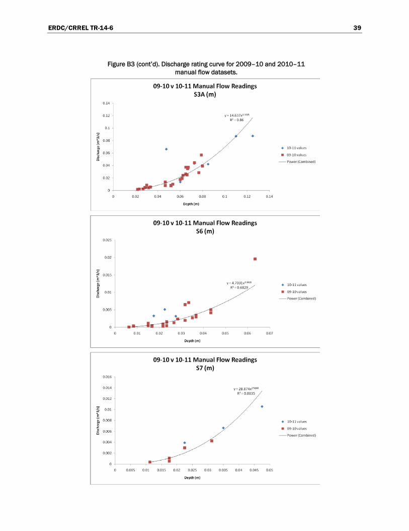
After graphing both years’ data on the same plot, the S7 and S6 curves showed a much better correlation. The S7 data followed a more clearly de-fined curve with the support of the 2009–10 data, and S6 also showed a similar pattern. The S3A graph revealed a possible outlier for the manual data from 2010–11 at a depth of 0.04–0.05 m. The earlier problems with the S2B data were further outlined in this graph as the 2009–10 values clearly supported the lower discharge readings from 2010–11. The S2B da-ta showed a similar trend for both datasets with the exception of the aforementioned outlier at the greatest depth and greatest discharge. The S1 graph revealed a possible outlier for the 2010–11 data at the greatest


depth and discharge. The data from austral summer 2010–11 also showed higher discharges than the previous austral summer.

Figure B3. Discharge rating curve for 2009–10 and 2010–11 manual flow datasets.


Figure B3 (cont’d). Discharge rating curve for 2009–10 and 2010–11 manual flow datasets.


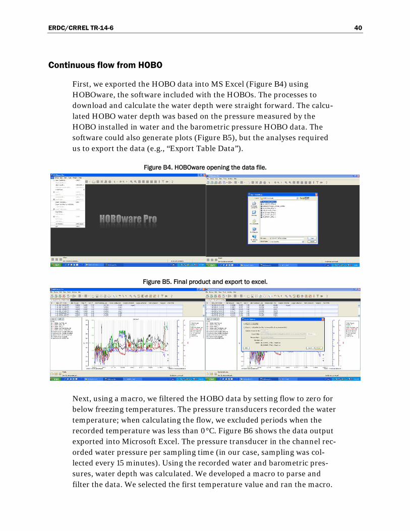
Continuous flow from HOBO

First, we exported the HOBO data into MS Excel (Figure B4) using HOBOware, the software included with the HOBOs. The processes to download and calculate the water depth were straight forward. The calcu-lated HOBO water depth was based on the pressure measured by the HOBO installed in water and the barometric pressure HOBO data. The software could also generate plots (Figure B5), but the analyses required us to export the data (e.g., “Export Table Data”).

Figure B4. HOBOware opening the data file.

Figure B5. Final product and export to excel.

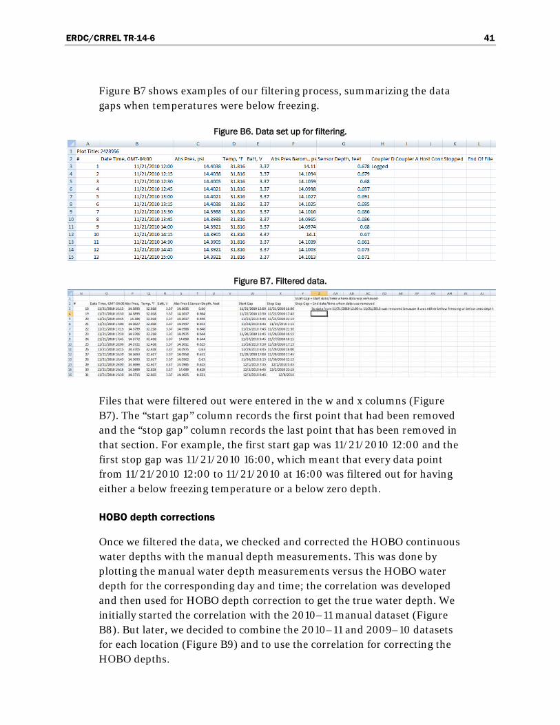
Next, using a macro, we filtered the HOBO data by setting flow to zero for below freezing temperatures. The pressure transducers recorded the water temperature; when calculating the flow, we excluded periods when the recorded temperature was less than 0°C. Figure B6 shows the data output exported into Microsoft Excel. The pressure transducer in the channel rec-orded water pressure per sampling time (in our case, sampling was col-lected every 15 minutes). Using the recorded water and barometric pres-sures, water depth was calculated. We developed a macro to parse and filter the data. We selected the first temperature value and ran the macro.


Figure B7 shows examples of our filtering process, summarizing the data gaps when temperatures were below freezing.

Figure B6. Data set up for filtering.

Figure B7. Filtered data.

Files that were filtered out were entered in the w and x columns (Figure B7). The “start gap” column records the first point that had been removed and the “stop gap” column records the last point that has been removed in that section. For example, the first start gap was 11/21/2010 12:00 and the first stop gap was 11/21/2010 16:00, which meant that every data point from 11/21/2010 12:00 to 11/21/2010 at 16:00 was filtered out for having either a below freezing temperature or a below zero depth.

HOBO depth corrections

Once we filtered the data, we checked and corrected the HOBO continuous water depths with the manual depth measurements. This was done by plotting the manual water depth measurements versus the HOBO water depth for the corresponding day and time; the correlation was developed and then used for HOBO depth correction to get the true water depth. We initially started the correlation with the 2010–11 manual dataset (Figure B8). But later, we decided to combine the 2010–11 and 2009–10 datasets for each location (Figure B9) and to use the correlation for correcting the HOBO depths.


Figure B8. Example of HOBO depth correction for 2010–11 data at S1 location.

y = 0.0374x + 0.1536R² = 0.0252

0

0.05

0.1

0.15

0.2

0.25

0.3

0.35

0.4

0 0.2 0.4 0.6 0.8 1 1.2 1.4 1.6

Man

ual D

epth

s (ft

)

HOBO Depths at the same time (ft)

S1 Manual v HOBO Depths (ft)


Figure B9. 2009–10 and 2010–11 datasets for HOBO depth correction.


Figure B9 (cont’d). 2009–10 and 2010–11 datasets for HOBO depth correction.

Seasonal continuous flow

After the HOBO depth correction equations were performed for each loca-tion, we applied the discharge rating curve equations for the 2010–11 da-


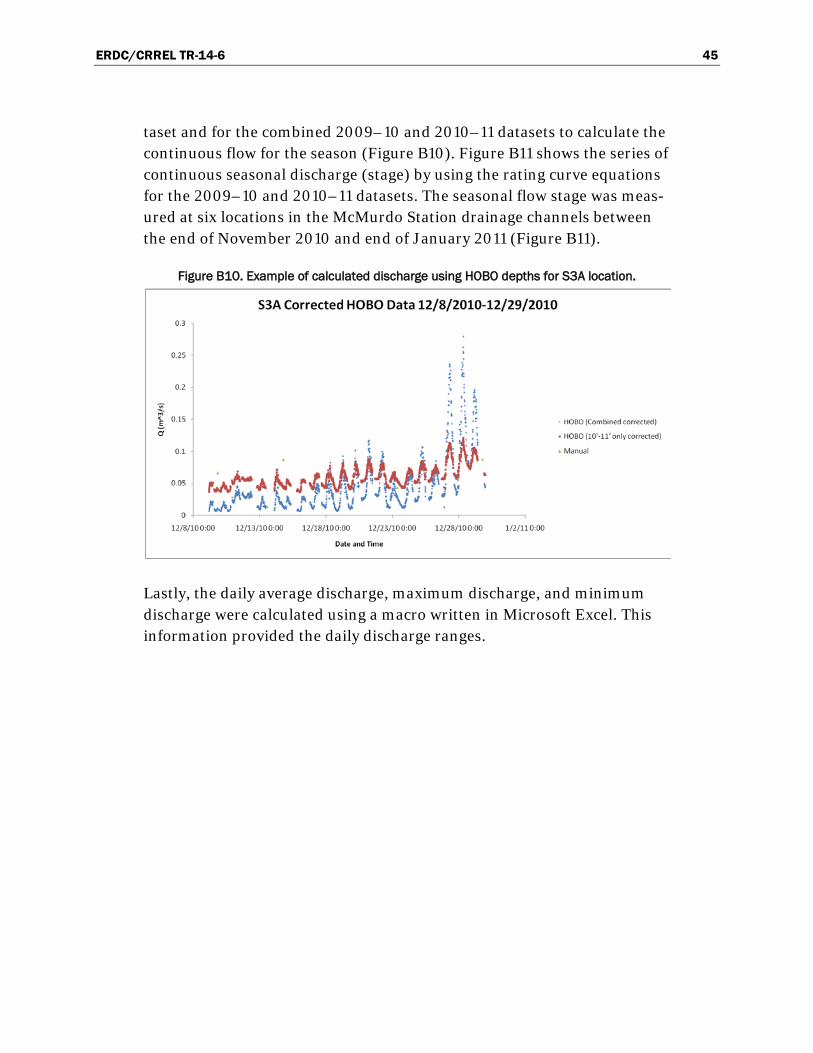
taset and for the combined 2009–10 and 2010–11 datasets to calculate the continuous flow for the season (Figure B10). Figure B11 shows the series of continuous seasonal discharge (stage) by using the rating curve equations for the 2009–10 and 2010–11 datasets. The seasonal flow stage was meas-ured at six locations in the McMurdo Station drainage channels between the end of November 2010 and end of January 2011 (Figure B11).

Figure B10. Example of calculated discharge using HOBO depths for S3A location.

Lastly, the daily average discharge, maximum discharge, and minimum discharge were calculated using a macro written in Microsoft Excel. This information provided the daily discharge ranges.


Figure B11. Estimated continuous flow at each location during austral summer 2010–11.

0

0.02

0.04

0.06

0.08

0.1

0.12

0.14

0.16

Hobo

Dis

char

ge (m

^3/s

)

Date and Time

S1

Manual(2.319874*Depth)^2

0.00

0.20

0.40

0.60

0.80

1.00

1.20

Hobo

Dis

char

ge (m

^3/s

)

Date and Time

S2B

Manual

0

0.05

0.1

0.15

0.2

0.25

0.3

0.35

0.4

0.45

0.5

Hobo

Dis

char

ge (m

^3/s

)

Date and Time

S2C



Figure B11 (cont’d). Estimated continuous flow at each location during austral summer 2010–11.

0.00

0.02

0.04

0.06

0.08

0.10

0.12

0.14

0.16

0.18

0.20

Hobo

Dis

char

ge (m

^3/s

)

Date and Time

S3A


0.000

0.001

0.002

0.003

0.004

0.005

0.006

Hobo

Dis

char

ge (m

^3/s

)

Date and Time

S6

Manual

0.000

0.005

0.010

0.015

0.020

0.025

0.030

0.035

Hobo

Dis

char

ge (m

^3/s

)

Date and Time

S7

Manual

(2.319874*Depth)^2

REPORT DOCUMENTATION PAGE Form Approved

OMB No. 0704-0188 Public reporting burden for this collection of information is estimated to average 1 hour per response, including the time for reviewing instructions, searching existing data sources, gathering and maintaining the data needed, and completing and reviewing this collection of information. Send comments regarding this burden estimate or any other aspect of this collection of information, including suggestions for reducing this burden to Department of Defense, Washington Headquarters Services, Directorate for Information Operations and Reports (0704-0188), 1215 Jefferson Davis Highway, Suite 1204, Arlington, VA 22202-4302. Respondents should be aware that notwithstanding any other provision of law, no person shall be subject to any penalty for failing to comply with a collection of information if it does not display a currently valid OMB control number. PLEASE DO NOT RETURN YOUR FORM TO THE ABOVE ADDRESS. 1. REPORT DATE (DD-MM-YYYY)

13-05-2014 2. REPORT TYPE

Technical Report/Final 3. DATES COVERED (From - To)

4. TITLE AND SUBTITLE


5a. CONTRACT NUMBER

5b. GRANT NUMBER

5c. PROGRAM ELEMENT NUMBER

6. AUTHOR(S)

Rosa T. Affleck, Meredith Carr, Margaret Knuth, Laura Elliot, Corey Chan, and Michael Diamond

5d. PROJECT NUMBER

5e. TASK NUMBER EP-ANT-11-04

5f. WORK UNIT NUMBER

7. PERFORMING ORGANIZATION NAME(S) AND ADDRESS(ES) 8. PERFORMING ORGANIZATION REPORT NUMBER

Cold Regions Research and Engineering Laboratory (CRREL) US Army Engineer Research and Development Center 72 Lyme Road Hanover, NH 03755-1290

ERDC/CRREL TR-14-6

9. SPONSORING / MONITORING AGENCY NAME(S) AND ADDRESS(ES) 10. SPONSOR/MONITOR’S ACRONYM(S)

National Science Foundation, Office of Polar Programs, Antarctic Infrastructure and Logistics Arlington, VA 22230

NSF 11. SPONSOR/MONITOR’S REPORT NUMBER(S)

12. DISTRIBUTION / AVAILABILITY STATEMENT Approved for public release; distribution is unlimited.

13. SUPPLEMENTARY NOTES

Engineering for Polar Operations, Logistics and Research (EPOLAR) 14. ABSTRACT As the austral summer approaches, major flow arteries are manually cleared in anticipation of the ephemeral runoff during the summer months. This flow, primarily from snowmelt, has daily and seasonal fluctuations. The flow fluctuation and variation depend on the air temperature and on many other factors. In addition, the runoff mobilizes sediment and localized soil contaminants that wash through these channels and discharge primarily into Winter Quarters Bay.

This report quantifies the runoff characteristics, including discharge correlations and variations for McMurdo Station drainage channels, and expands our understanding on the runoff charactestics at McMurdo Station. The flow data taken during austral summer 2010–11 combined with 2009–10 data fills the gaps in the analysis to quantify the runoff. Based on the correlation between the change in accumulated thawing degree days and cloudiness expressed in clearness, the time delay in the peak discharge can occur between 4 and 14 days after a peak temperature. Based on the frequency and probability distribution of the flow, a flow greater than 0.33 m3/s in the major channel occurred less than 5% of the time during the season. This study provides critical information for planning, operation and maintenance, the design of preventive methods, and the application of best practices.

15. SUBJECT TERMS Drainage Erosion

McMurdo Station Runoff Seasonal discharge

Snowmelt

16. SECURITY CLASSIFICATION OF: 17. LIMITATION OF ABSTRACT

18. NUMBER OF PAGES

19a. NAME OF RESPONSIBLE PERSON

a. REPORT

U

b. ABSTRACT

U

c. THIS PAGE

U None 58 19b. TELEPHONE NUMBER (include area code)

Standard Form 298 (Rev. 8-98) Prescribed by ANSI Std. 239.18

Documents

ERDC/CRREL TR-14-6 'Runoff characterization and variations ... · 10 Discharge rating curve from all manual measurement for seasons 2009 –10 and 2010–11, generating equation (8)