Equivalent One-Dimensional Spring-Dashpot System ... Computer Modeling in Engineering & Sciences, Vol. 67, No. 3, pp. 211-238, 2010 Equivalent One-Dimensional Spring-Dashpot System

CMES: Computer Modeling in Engineering & Sciences, Vol. 67, No. 3, pp. 211-238, 2010

Equivalent One-Dimensional Spring-Dashpot System Representing Impedance Functions of Structural Systems with

Non-Classical Damping

M. Saitoh1

Abstract This paper describes the transformation of impedance functions in general structural systems with non-classical damping into a one-dimensional spring-dashpot system (1DSD). A transformation procedure based on complex modal analysis is proposed, where the impedance function is transformed into a 1DSD comprising units arranged in series. Each unit is a parallel system composed of a spring, a dashpot, and a unit having a spring and a dashpot arranged in series. Three application examples are presented to verify the applicability of the proposed procedure and the accuracy of the 1DSDs. The results indicate that the 1DSDs accurately simulate the impedance functions for a spring-dashpot-mass structure, a truss frame structure, and a plate structure. The 1DSD transformation offers compatibility with complex modal analysis: a large number of units associated with high modes beyond a target frequency region can be removed from the 1DSDs as an approximate expression of impedance functions. The accuracy of the approximated 1DSDs can be improved by incorporating an additional unit associated with the residual stiffness that compensates for the effect of high modes. A marked decrease in the computational domain size and time with the use of the 1DSDs is of great scientific and engineering importance in diverse technological applications.

Keywords: Impedance functions, lumped parameter models, one-dimensional spring-dashpot system, non-classical damping, dynamic response, residual stiffness.

1 Introduction

Efficient reduction of degrees of freedom (DOFs) in structural systems is of great importance for solving dynamic problems, as numerous degrees of freedom are typically used to accurately describe structural systems by using discretized elements such as mass-spring elements, rod/beam elements, and isoparametric elements. In particular, a proper reduction of the DOFs is strongly demanded for solving dynamic problems where structural systems interact with dynamic systems having an extremely large number of DOFs, such as vehicles, industrial machines, and robots. In such problems, the total number of DOFs is enormous, so the computational domain and time tend to be extremely large.

1 Saitama University, Saitama, Japan.


The dynamic stiffness method (DSM) has frequently been used to reduce the DOFs in structural systems, especially for beam-like structures [e.g., Kolousek (1973), Hizal and Gürgöze (1998), Barros and Luco (1990), Wolf (1994, 1997), Wu and Lee (2002)]. Since this method was first developed in the early 1940s by Kolousek (1941), it has been applied to various vibration analyses and has been appreciably improved to overcome difficulties in diverse vibration problems. The global dynamic stiffness generated in the DSM procedure and various improved DSMs can be used as reduced systems that express the dynamic stiffness or a so-called impedance function at the structural interface of the contact point with dynamic systems. In general, the reduced systems representing impedance functions transformed by DSMs show a significant decrease in the number of DOFs from the original structural systems. Most impedance functions are known to show strong frequency-dependent characteristics: the real part of the impedance functions represents the stiffness characteristics, whereas the imaginary part represents the damping characteristics. The reduced systems are applicable to interaction problems whenever the dynamic systems act under linearly elastic conditions. However, the use of reduced systems expressed in terms of the excitation frequency has presented serious problems when nonlinearities such as slippage, separation, cracking, yielding, and collapse occur in the dynamic systems. A mechanical representation is one way to break through this problem. Impedance functions are generally represented using a lumped parameter model (LPM) comprising springs, dashpots, and masses. Although each element has a frequency-independent coefficient, a particular combination of elements allows simulation of a frequency-dependent impedance characteristic. Thus, LPMs can easily be incorporated into a conventional numerical analysis in the time domain even under nonlinear conditions in dynamic systems. Hizal and Gürgöze (1998) proposed an LPM of a longitudinally vibrating elastic rod with a viscous damping element placed mid-span; LPMs for the interface of three-dimensional wave propagation continua have been developed (e.g., Barros and Luco (1990), Wolf (1994, 1997), Wu and Lee (2002), Andersen (2008), and Saitoh (2007)). To the best of the author’s knowledge, however, the number of studies proposing LPMs for structural systems is very limited, and LPMs that represent the impedance functions in structural systems with general damping have never been proposed. This study shows that the impedance functions of general structural systems with non-classical damping can be represented by a one-dimensional spring-dashpot system (1DSD); a transformation procedure into 1DSDs is proposed based on conventional complex modal analysis. The advantage of this 1DSD representation is comparable to the advantage of conventional modal analysis: an approximate expression of the impedance functions can be obtained using 1DSDs with an appreciably reduced number of units associated with related modes in a target frequency region instead of using a large number of units associated with high modes beyond the target frequency region. The objectives of this study are: 1) To propose a procedure for formulating 1DSDs using complex modal analysis; 2) to verify the accuracy of the transformed 1DSDs compared with a direct solution using the original structural systems through three example applications to a mass-spring-dashpot structure, a truss frame structure, and a plate


structure; and 3) to show an example where the number of DOFs in a 1DSD representing the impedance function of a cantilever plate having 240 DOFs can be significantly reduced.

2 Transformations of Impedance Functions in General Structural Systems into 1DSDs

2.1 General expressions of impedance functions in structural systems with non-classical damping based on complex modal analysis

A structural system comprising N DOFs is considered. The equations of motion of the original structural systems with damping can be generally described by

[ ]{ } [ ]{ } [ ]{ } { }puKuCuM =++ &&& , (1)

where [ ]M , [ ]C , and [ ]K are the mass matrix, damping matrix, and stiffness matrix, respectively, of the original structural systems. Each matrix has the order NN × ; { }u and { }p are the response displacements and the external forces at the nodes, respectively, and each vector has the order N . The dots denote partial derivatives with respect to time t . In Eq. 1, the mass matrix [ ]M is symmetric and positive definite; the damping matrix [ ]C and the stiffness matrix [ ]K are symmetric and non-negative definite, respectively. In this study, the damping matrix [ ]C is assumed to be based on non-classical damping. Therefore, Eq. 1 cannot be decoupled using the undamped modal vectors of the structural system. In the following, therefore, a well-known procedure based on complex modal analysis (e.g., Foss (1958)) is applied to obtain the impedance function of the systems. Nagamatsu (1985) described detailed procedures for obtaining the general form of the admittance functions (the inverse of the impedance functions) of the structural systems based on complex modal analysis. Therefore, in the following, the general impedance function in structural systems is derived according to his procedure. In complex modal analysis, the following N2 first-order equations are considered instead of N second-order equations of Eq. 1:

[ ]{ } [ ]{ } { }fzSzR =+& , (2)

where

[ ] [ ] [ ][ ] [ ] ⎥⎦

⎤⎢⎣

⎡=

0MMC

R , [ ] [ ] [ ][ ] [ ]⎥⎦

⎤⎢⎣

⎡−

=M

KS

00

, { } { }{ }⎭

⎬⎫

⎩⎨⎧

=uu

z&

, { } { }{ }⎭

⎬⎫

⎩⎨⎧

=0p

f .

To obtain the homogeneous solution of Eq. 2, let

{ } { }Φ= tez λ . (3)

This yields


[ ] [ ]( ){ } { }0=Φ+ SRλ . (4)

The solution of Eq. 4 will yield 2N eigenvalues and eigenvectors nλ and

{ } { } { }{ }Tnnnn φλφ=Φ , Nn 2,,2,1 L= .

For a stable system, each nλ is either real and negative (this is associated with an over-damped mode) or complex with a negative real part (this is associated with an under-damped mode). Each complex eigenvalue nλ is known to have an eigenvalue nλ that is the complex conjugate of nλ ; the corresponding vector { }nφ has a vector { }nφ whose components are complex conjugates of those of { }nφ . The eigenvectors { }nΦ are also known to satisfy the following orthogonality relations:

{ } [ ] { } 0=ΦΦ nT

m R , when nm ≠ (5)

{ } [ ] { } 0=ΦΦ nT

m S , when nm ≠ . (6)

The eigenvectors are assembled compactly into a matrix using diagonal matrices [ ]Ω and [ ]Ω comprising the eigenvalues nλ and nλ , respectively, as

[ ] [ ] [ ][ ][ ] [ ][ ]⎥⎦

⎤⎢⎣

⎡

ΩΩ=Ψ

φφφφ

, (7)

where

[ ] { } { } { }[ ]Nφφφφ L21= ,

[ ] { } { } { }[ ]Nφφφφ L21= ,

[ ] [ ]ndiag λ=Ω , Nn ,,2,1 L= ,

[ ] [ ]ndiag λ=Ω , Nn ,,2,1 L= .

The matrix [ ]Ψ is called the modal matrix. Non-homogeneous solutions of Eq. 2 can be expressed using a modal series based on the orthogonality relations:

( ){ } [ ] ( ){ }ttz ξΨ= . (8)

Here, the new coordinates ( ){ }tξ are called the modal coordinates. Substituting Eq. 8 into Eq. 2 and premultiplying the equation by [ ]TΨ yields

[ ] [ ][ ]{ } [ ] [ ][ ]{ } [ ] { }fSR TTT Ψ=ΨΨ+ΨΨ ξξ& . (9)

The orthogonality relations, Eqs. 5 and 6, indicate that [ ] [ ][ ]ΨΨ RT and [ ] [ ][ ]ΨΨ ST are diagonal matrices. The upper N components of the matrices are denoted as nα and nβ , respectively; the lower N components are complex conjugates of nα and nβ ,


respectively, denoted as nα and nβ . These diagonal matrices [ ] [ ][ ]ΨΨ RT and [ ] [ ][ ]ΨΨ ST are denoted as [ ]α and [ ]β , respectively. Substituting Eqs. 3 and 8 into the homogeneous equation of Eq. 2 and premultiplying the result by [ ]TΨ clearly yields

nnn αβλ −= , (10)

nnn αβλ −= . (11)

In general, the eigenvalues nλ and nλ can be replaced by the expressions

dnnn iωσλ +−= , (12)

dnnn iωσλ −−= , (13)

where nσ is the n -th modal decay rate and dnω is the n -th damped natural circular frequency.

To obtain the impedance functions in structural systems, the harmonic external force and harmonic response function are assumed to be

{ } { } tieFf ω= or { } { } tiePp ω= , (14)

{ } { } tieZz ω= or { } { } tieUu ω= , (15)

where ω is the circular frequency and { }F , { }P , { }Z , and { }U are time-independent vectors. In this case, the modal coordinates ( ){ }tξ in Eq. 8 can be written in the form

( ){ } { } tiet ωξ Ξ= , (16)

where { }Ξ is a time-independent vector.

Substituting Eqs. 14, 15, and 16 into Eq. 2 and premultiplying the result by [ ]TΨ yields

[ ] [ ]( ){ } [ ] { }Fi TΨ=Ξ+ βαω . (17)

Substituting { }Ξ of Eq. 17 into Eq. 16 and the resultant modal coordinates ( ){ }tξ into Eq. 8 yields

{ } [ ] [ ] [ ]( ) [ ] { }FiZ TΨ+Ψ= −1βαω . (18)

Eq. 18 can be rewritten using Eq. 7 as

{ }{ }[ ]

[ ] [ ][ ][ ] [ ][ ]

[ ] [ ][ ] [ ]

[ ] [ ][ ][ ] [ ][ ]

{ }{ }⎭

⎬⎫

⎩⎨⎧⎥⎦

⎤⎢⎣

⎡

ΩΩ

⎥⎦

⎤⎢⎣

⎡⎥⎦

⎤⎢⎣

⎡

ΩΩ=

⎭⎬⎫

⎩⎨⎧

Ω 000 P

UU

TT

TT

φφφφ

γγ

φφφφ

. (19)


Here, [ ]γ and [ ]γ are diagonal matrices comprising the diagonal components ( )nni βωα +1 and ( )nni βαω +1 , respectively. The upper N equations are extracted

as follows:

{ } [ ][ ][ ] [ ][ ][ ]( ){ }PU TT φγφφγφ += . (20)

On the basis of Eq. 20, the admittance function IJH , defined as the ratio of the amplitude of the displacement response IU at the I-th DOF to a force JP applied at the J-th DOF, is expressed as

∑=

⎟⎟⎠

⎞⎜⎜⎝

⎛+

++

==N

n nn

nJnI

nn

nJnI

J

IIJ iiP

UH

1 βαωφφ

βωαφφ

, (21)

where nIφ and nJφ are the components of the n -th eigenvector at the I-th and J-th DOFs, respectively; nIφ and nJφ are the complex conjugates of the components nIφ and

nJφ , respectively. Substituting Eqs. 10–13 into Eq. 21 yields

( ) ( )∑=

⎟⎟⎠

⎞⎜⎜⎝

⎛++

−+

+−+

=N

n ndn

nn

ndn

nnIJ i

iRGi

iRGH

1 σωωσωω, (22)

where n

nJnInn iRG

αφφ

=+ andn

nJnInn iRG

αφφ

=− .

Accordingly, the impedance function IJS , defined as the ratio of the displacement response IU to the external force JP , is expressed by the inverse of Eq. 22 as

( ) ( )∑=

⎟⎟⎠

⎞⎜⎜⎝

⎛++

−+

+−+

===N

n ndn

nn

ndn

nnIJI

JIJ

iiRG

iiRGHU

PS

1

11

σωωσωω

. (23)

2.2 Exact procedure for transforming impedance functions into 1DSDs

To the best of the author’s knowledge, an exact mechanical representation of the impedance functions expressed by Eq. 23 has never been reported in the literature. In this section, an exact procedure for transforming impedance functions into an equivalent 1DSD is proposed. Instead of dealing with Eq. 23 directly, consider a renewed form comprising coupled terms, each created by the combination of the n -th two terms of the denominator in Eq. 23:


( )( )∑

= +−++−

= N

n ndnn

nndnnnIJ

iGiRG

S

1222 2

221

ωσωωσωωσ

. (24)

The above form can be rewritten as

∑=

= N

n nIJ

IJ

K

S

1

11

, (25)

where

( )( ) nndnnn

ndnnnIJ GiRG

iK

ωωσωσωωσ

222222

+−+−+

= . (26)

Eq. 25 implies that the impedance functions expressed by Eq. 24 could be transformed into a set of units arranged in series, where each unit has an impedance function expressed by Eq. 26. Note that a mechanical unit exactly representing the impedance function expressed by Eq. 26 could be found serendipitously by changing the configurations of the mechanical components.

In this study, the following mechanical representation for Eq. 26 is proposed: a parallel system comprising a spring Tnk , a dashpot Tnc , and a unit having a spring nk and a dashpot nc arranged in series as shown in Fig. 1. The impedance function of the proposed system is described by

TnTnn

n

n

n

Tn

Tn

Tn

n

Tnn

Tnn

n

ci

cck

ck

ck

ck

icckk

Kω

ωω

+

⎟⎟⎠

⎞⎜⎜⎝

⎛+++−

=

2

. (27)

The mathematical form of Eq. 27 is analogous to that of Eq. 26. The equivalency of each term of Eq. 26 with those of Eq. 27 yields

22dnnTnnTnn cckk ωσ += , (28)

nn

n

Tn

Tn

Tn

n

ck

ck

ck

σ2=++ , (29)

( )ndnnnTnnn RGcck ωσ −= 2 , (30)

nTn Gc 21 = . (31)


Jp

Iu

2Tc

2k

2Tk

2c

1Tc

1k

1Tk

1c

1−NTc

1−Nk

1−NTk

1−Nc

NTc

Nk

NTk

Nc

nTc

nk

nTk

nc

enf 1−

enw 1−

enf

enw

eng

env

(b)

(a)

nTce

nf 1−

enw 1−

enf

enw

(c)

nTk

Figure 1: (a) One-dimensional lumped parameter model with spring and dashpot elements (1DSDs) for simulating the impedance function ( ) IJIJ upS =ω in general structural systems. (b) Unit associated with under-damped mode and (c) unit associated with over-damped mode. Solving the simultaneous equations of Eqs. 28–31 for the springs nk , Tnk and the

dashpots nc , Tnc yields

( )dnnnn

dnnTn RG

kωσ

ωσ−+

=2

22

, (32)

nTn G

c2

1= , (33)

( )( )dnnnnn

dnnnn RGG

RGk

ωσω

−+−

= 2

222

2, (34)

( )( )2

222

2 dnnnnn

dnnnn RGG

RGc

ωσω

−

+−= . (35)

The above results indicate that the properties of the mechanical elements of the units can be determined from the modal quantities nσ , dnω , nG , and nR obtained by a one-time complex modal analysis calculation. Fig. 1 shows a 1DSD representing the impedance functions of general structural systems.


2.3 Transformations of impedance functions into 1DSDs with real eigenvalues (over-damped modes)

Eigenvalues nλ are real and negative when over-damped modes appear. In this case, Eqs. 32–35 cannot be used to construct a mechanical unit of impedance functions. When an eigenvalue nλ is real and negative, the second term of the denominator associated with the complex conjugates nJnI φφ in Eq. 23 does not exist. In addition, the imaginary part of the eigenvalue is found to be zero, whereas the imaginary part of the eigenvectors

Inφ and Jnφ also becomes zero, which results in 0=nR . Therefore, the impedance function associated with over-damped modes is expressed as follows:

n

n

n

nnIJ G

i

iG

Kσω

σω

+=

+

=1

. (36)

Accordingly, the following spring Tnk and dashpot Tnc comprise a Kelvin–Voigt unit, as shown in Fig. 1c for an over-damped mode.

n

nTn G

kσ

= (37)

nTn G

c 1= (38)

Note that over-damped modes generally appear with even numbers m2 in N2 modes, so the total unit number N in Eq. 25 changes to ( )mNN +=′ when over-damped modes exist.

2.4 Transformations of impedance functions in structural systems with classical damping

Classical damping (proportional damping) is a specific damping system wherein the damping matrix is proportional to the stiffness matrix, the mass matrix, or both. In transforming the impedance functions of structural systems with classical damping, Eq. 1 can be decoupled using the undamped modal vectors of the structural systems. The decoupling of Eq. 1 by using undamped modal vectors shows that nG in Eq. 26 becomes zero (c.f. Nagamatsu (1985)); hence, Eq. 26 becomes

( )ndn

ndnnnIJ R

iK

ωωσωωσ

22222

−+−+

= . (39)

The mathematical form of Eq. 39 is incompatible with that of Eq. 27. This implies that the 1DSD proposed here is limited to structural systems with non-classical damping. In addition, a damping system that is mostly classical but partially non-classical due to additional dashpots, for instance, may generate the particular modes associated with


proportional damping. In this case, the proposed 1DSDs are unavailable for the units corresponding to the modes. A possible technique to transform the systems into a one-dimensional equivalent mechanical system would be to change Eq. 39 into the following form:

ngngngnIJ kicmK ++−= ωω 2 , (40)

where

ndnng R

mω2

1−= , (41)

nnd

nng R

cωσ

−= , (42)

nnd

ndnng R

kω

ωσ2

22 +−= . (43)

Eq. 40 indicates that a unit associated with classical damping can be considered as a parallel system consisting of a spring ngk , a dashpot ngc , and an element ngm having the same dimensions as ordinary mass. Herein, the element ngm should generate a reaction force proportional to the relative acceleration of the two nodes between which it is placed. This element is termed “gyro mass,” and was first proposed and initially used for expressing frequency-dependent impedance functions by Saitoh (2007). Although the use of the gyro mass in structural systems with classical damping is beyond the scope of this study, this description could be valuable in further studies to solve this problem.

2.5 Matrix expressions of 1DSDs for numerical computations

In the matrix representation of 1DSDs proposed above, which is convenient for numerical computations, the relationship between the displacements ( e

nw 1− , enw , and e

nv ) and the external forces ( e

nf 1− , enf , and e

ng ) at both ends and at the internal node of a unit associated with the n -th mode, as shown in Fig. 1b, can be written as

{ } [ ] { } [ ] { } ne

nene

nene WKWCF += & , (44)

where

{ } { }Ten

en

enn

e fgfF 1−= , (45)

{ } { }Ten

en

enn

e wvwW 1−= , (46)


[ ]⎥⎥⎥

⎦

⎤

⎢⎢⎢

⎣

⎡

−

−+

⎥⎥⎥

⎦

⎤

⎢⎢⎢

⎣

⎡−

−=

TnTn

TnTn

nn

nn

ne

kk

kkkkkk

K0

0000

00000

, (47)

[ ]⎥⎥⎥

⎦

⎤

⎢⎢⎢

⎣

⎡

−

−+

⎥⎥⎥

⎦

⎤

⎢⎢⎢

⎣

⎡

−−=

TnTn

TnTn

nn

nnne

cc

cc

ccccC

0000

0

00

000. (48)

[ ] neK and [ ] neC are the stiffness matrix and damping matrix, respectively, of a unit associated with the n -th mode. Superimposing the stiffness matrices and damping matrices of all units gives the simultaneous equations of motion of a 1DSD expressed as a matrix. When over-damped modes appear in the systems, a DOF for the internal node in the unit and the two connected elements nk and nc are removed, as shown in Fig. 1c.

3 Example Applications

3.1 Example 1: One-dimensional mass-spring-dashpot system

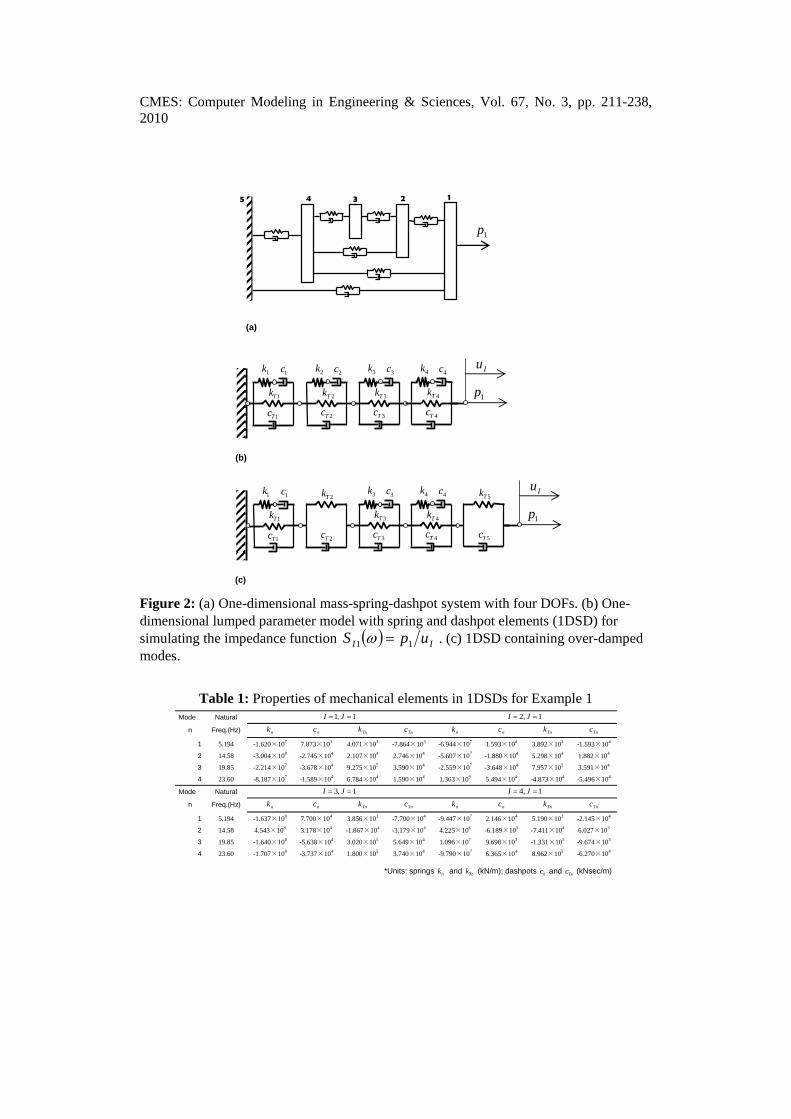
Fig. 2 shows a one-dimensional four-DOF mass-spring-damper system. The four masses are connected with seven springs and seven dampers as shown in the figure. The numbers in the figure indicate the nodal numbers of this structural model. The properties of the masses are: 0.14321 ==== mmmm ton, where im is defined as the mass at the i-th node. The spring constants are =12k 38.0 10× kN/m, === 453423 kkk 3100.4 × kN/m,

=24k 3100.3 × kN/m, =14k 3100.2 × kN/m, and =15k 3100.1 × kN/m. The damping coefficients of the dashpots are ===== 1424342312 ccccc 0.2 kN-sec/m and

== 1545 cc 0.4 kN-sec/m. Here, ijk and ijc are the constants of a spring and a dashpot, respectively, placed between the i-th and j-th nodes. The fifth node is fixed in the horizontal direction. The equations of motion for the mass-spring-dashpot system (Eq. 1) can be constructed using conventional techniques (c.f. Weaver, Timoshenko, and Young (1990)). Table 1 shows the properties of the elements in the 1DSDs obtained by the procedure described above. This example investigates the impedance functions associated with the displacement response at nodes 1, 2, 3, and 4 when node 1 is excited. The results of modal analysis indicate that no over-damped mode exists in the system. Thus, four units comprise the 1DSDs, as shown in Table 1 for this case. Fig. 3 shows the impedance functions of the 1DSDs and the impedance functions evaluated directly from Eq. 1 of the original four-DOF mass-spring-dashpot system. Fig. 3 indicates that the impedance functions of the 1DSDs are identical to those evaluated from the original mass-spring-dashpot system. Consider a mass-spring-dashpot system showing over-damped modes as a possible case in practical applications. The same system is used here except that the damping


1Tc

1k

1Tk

1c

1p

Iu

3Tc

3k

3Tk

3c

4Tc

4k

4Tk

4c

(b)

(a)

2Tc

2k

2Tk

2c

1Tc

1k

1Tk

1c

1 2 3 4

1p

5

1p

Iu

3Tc

3k

3Tk

3c

4Tc

4k

4Tk

4c

(c)

2Tk

2Tc

5Tk

5Tc

Figure 2: (a) One-dimensional mass-spring-dashpot system with four DOFs. (b) One-dimensional lumped parameter model with spring and dashpot elements (1DSD) for simulating the impedance function ( ) II upS 11 =ω . (c) 1DSD containing over-damped modes.

Table 1: Properties of mechanical elements in 1DSDs for Example 1 Mode Natural 1,1 == JI 1,2 == JI

n Freq.(Hz) nk nc Tnk Tnc nk nc Tnk Tnc

1 5.194 -1.620×107 7.873×103 4.071×103 -7.864×103 -6.944×107 1.593×104 3.892×103 -1.593×104

2 14.58 -3.004×108 -2.745×104 2.107×104 2.746×104 -5.607×107 -1.880×104 5.298×104 1.882×104

3 19.85 -2.214×107 -3.678×104 9.275×105 3.590×104 -2.559×107 -3.648×104 7.957×105 3.591×104

4 23.60 -8.187×107 -1.589×104 6.784×104 1.590×104 1.363×109 5.494×104 -4.873×104 -5.496×104

Mode Natural 1,3 == JI 1,4 == JI


1 5.194 -1.637×109 7.700×104 3.856×103 -7.700×104 -9.447×107 2.146×104 5.190×103 -2.145×104

2 14.58 4.543×108 3.178×104 -1.867×104 -3.179×104 4.225×106 -6.189×103 -7.411×104 6.027×103

3 19.85 -1.640×108 -5.638×104 3.020×105 5.649×104 1.096×107 9.698×103 -1.331×105 -9.674×103

4 23.60 -1.707×108 -3.737×104 1.800×105 3.740×104 -9.790×107 6.365×104 8.962×105 -6.270×104 *Units: springs nk and Tnk (kN/m); dashpots nc and Tnc (kNsec/m)


coefficient in the dashpot, =34c 0.2 kN-sec/m, is changed to 2100.2 × kN-sec/m. The results of modal analysis indicate that the third and eighth modes in 2N ( 8= ) vibrating modes become over-damped modes where the eigenvalues are real and negative, whereas the eigenvalues of the other six modes become three sets of complex conjugates. Hence, a total of five units comprise the 1DSDs representing the impedance functions in the mass-spring-dashpot system, as shown in Fig. 2c. Table 2 shows the properties of the elements in the 1DSDs. Fig. 4 shows the impedance functions of the 1DSDs with over-damped modes and the impedance functions evaluated directly from Eq. 1 of the original system. The impedance functions of the 1DSDs are compatible with those evaluated from the original system.

0 5 10 15 20 25 30

-1.5

-1.0

-0.5

0.0

0.5

1.0

1.5

<Original System> I=1,J=1 I=2,J=1 I=3,J=1 I=4,J=1

( x105 )

Re

(S I

J )

Frequency (Hz)0 5 10 15 20 25 30

-1.5

-1.0

-0.5

0.0

0.5

1.0

1.5

<1DSDs> I=1,J=1 I=2,J=1 I=3,J=1 I=4,J=1

( x105 )

Im (S

I J )

Frequency (Hz)(a) (b)

Figure 3: Impedance functions of a one-dimensional mass-spring-dashpot system using 1DSDs [(a) real part and (b) imaginary part]. Results obtained from the original mass-spring-dashpot system are shown for comparison.

0 5 10 15 20 25 30

-0.6

-0.4

-0.2

0.0

0.2

0.4

0.6

<Original System> I=1,J=1 I=2,J=1 I=3,J=1 I=4,J=1

( x105 )

Re

(S I

J )

Frequency (Hz)0 5 10 15 20 25 30

-0.2

0.0

0.2

0.4

0.6

0.8

<1DSDs> I=1,J=1 I=2,J=1 I=3,J=1 I=4,J=1

( x105 )

Im (S

I J )


Figure 4: Impedance functions of a one-dimensional mass-spring-dashpot system using 1DSDs with over-damped modes [(a) real part and (b) imaginary part]. Results obtained from the original mass-spring-dashpot system are shown for comparison.


Table 2: Properties of mechanical elements in 1DSDs for Example 1 with over-damped modes



1 5.347 -5.635×108 -4.461×104 3.987×103 4.462×104 -9.938×107 1.849×104 3.879×103 -1.847×104

2 5.743 - - 1.156×106 3.203×104 - - 4.775×105 1.323×104

3 15.42 -3.479×107 9.324×103 2.337×104 -9.293×103 -7.872×109 2.207×105 5.806×104 -2.207×105

4 23.55 -1.079×108 -1.847×104 6.927×104 1.849×104 1.561×109 5.886×104 -4.860×104 -5.888×104

5 58.15 - - -3.278×109 -8.973×106 - - 4.110×109 1.125×107



1 5.347 -4.687×105 1.337×103 4.219×103 -1.310×103 -1.491×106 -2.522×103 4.832×103 2.530×103

2 5.743 - - 1.083×105 3.002×103 - - -3.105×105 -8.605×103

3 15.42 2.503×106 -2.774×103 -2.822×104 2.714×103 5.704×106 4.186×103 -2.889×104 -4.195×103

4 23.55 -3.538×107 -2.069×104 2.643×105 2.065×104 -1.067×108 3.634×104 2.694×105 -3.614×104

5 58.15 - - 2.766×107 7.570×104 - - -2.823×107 -7.727×104

*Units: springs nk and Tnk (kN/m); dashpots nc and Tnc (kNsec/m)

3.2 Example 2: Two-dimensional truss frame system with damping

Fig. 5 shows a two-dimensional truss frame system with six DOFs with damping. The fourth and fifth nodes are fixed in the vertical and horizontal directions. The structural model comprises seven rod elements. Each rod has a cross-sectional area 01.0=tA m2 and elastic modulus 61000.1 ×=tE kN/m2; the mass density of rods 3 and 4 is

00.4=tρ ton/m3, and that of the other five rods is 00.2=tρ ton/m3. In the system, a conventional rod element is used with a consistent mass that can carry only axial loads (c.f. Weaver, Timoshenko, and Young (1990)). In this example, the damping matrix for each rod element is constructed on the basis of

[ ] [ ]kkk KC β= , (49)

where

1

2ωζ

β kk = , (50)

where [ ]kC and [ ]kK are the damping matrix and stiffness matrix, respectively, of the k-th rod element; the parameter kζ is the damping ratio of the k-th rod at the fundamental natural frequency of the structural system, and 1ω is the fundamental natural circular frequency of the undamped system. In this example, the damping ratio of rods 1, 6, and 7 is 0.02, whereas that of rods 2, 3, 4, and 5 is 0.01. 1ω ( 1.212= rad/sec) is estimated using conventional modal analysis without damping.


(b)

(a)

1p

Iu

5Tc

5k

5Tk

5c

6Tc

6k

6Tk

6c

2Tc

2k

2Tk

2c

1Tc

1k

1Tk

1c

1 2 1p

3 4 5

1m

2m 2m

1m 2m

6=k

1=k

2=k 3=k 4=k 5=k

7=k

Figure 5: (a) Truss frame system with six DOFs with damping. (b) One-dimensional lumped parameter model with spring and dashpot elements (1DSD) for simulating the impedance function ( ) II upS 11 =ω .

Table 3: Properties of mechanical elements in 1DSDs for Example 2



1 33.75 -9.523×107 9.047×103 3.862×104 -9.038×103 9.523×107 -9.047×103 -3.862×104 9.038×103

2 45.43 -7.340×107 -3.622×103 1.457×104 3.623×103 -7.340×107 -3.622×103 1.457×104 3.623×103

3 96.34 -1.178×108 3.456×103 3.710×104 -3.451×103 -1.178×108 3.456×103 3.710×104 -3.451×103

4 148.5 -5.153×108 -7.281×104 8.919×106 7.252×104 -5.153×108 -7.281×104 8.919×106 7.252×104

5 153.3 -1.341×107 9.411×102 6.056×104 -9.292×102 1.341×107 -9.411×102 -6.056×104 9.292×102

6 194.9 -8.074×106 -8.420×102 1.317×105 8.426×102 8.074×106 8.420×102 -1.317×105 -8.426×102

Mode Natural 1,3 == JI

n Freq.(Hz) nk nc Tnk Tnc

1 33.75 6.478×1020 3.957×1018 -4.120×1020 -1.500×1018

2 45.43 -3.438×109 2.453×104 1.427×104 -2.453×104

3 96.34 3.537×108 -7.171×103 -5.322×104 7.164×103

4 148.5 1.168×108 1.010×104 -7.618×105 -1.012×104

5 153.3 2.892×1019 1.462×1017 -2.843×1019 -6.055×1015

6 194.9 -4.882×1020 1.180×1019 4.855×1020 -1.341×1016


Table 3 shows the properties of the elements in the 1DSDs obtained by the proposed procedure. In this example, the impedance functions associated with the displacement response at nodes 1, 2, and 3 in the horizontal direction when node 1 is excited in the same direction are discussed. No over-damped modes exist in this system. Table 3 shows that extremely large coefficients for certain elements exist in the 1DSDs, which is caused by the markedly small nJnIφφ and nJnIφφ components of the eigenvectors. In this case, the displacements of these units are considered to be negligibly small in the 1DSDs. Therefore, reduced 1DSDs consisting of units excluding the shaded units are used to approximately express the impedance functions. In this example, the above reduction of


units is attributed mainly to the symmetry in the shape and material properties of the structural system. In particular, nodes located on the line of symmetry of the system tend to show extremely small components of the eigenvectors for particular modes. Therefore, it is conceivable that the above reduction may not be generally expected in realistic structural systems having asymmetric shapes and properties. Fig. 6 compares the impedance functions from the 1DSDs and those evaluated directly from Eq. 1 for the truss frame system. It is clear that they are in close agreement.

0 50 100 150 200

-1.0

-0.5

0.0

0.5

1.0

1.5

2.0

<Original System> I=1,J=1 I=2,J=1 I=3,J=1

( x105 )

Re

(S I

J )

Frequency (Hz)0 50 100 150 200

-2.0

-1.5

-1.0

-0.5

0.0

0.5

1.0

1.5

<1DSDs> I=1,J=1 I=2,J=1 I=3,J=1

( x105 )

Im (S

I J )


Figure 6: Impedance functions of a two-dimensional truss frame system using 1DSDs [(a) real part and (b) imaginary part]. Results obtained from the original truss frame system are shown for comparison.

3.3 Example 3: Two-dimensional cantilever plate system with damping

Fig. 7 shows a two-dimensional plate system with eight DOFs with damping. Nodes 5, 6, 7, and 8 are fixed in the vertical and horizontal directions. The structural system comprises three conventional rectangular isoparametric elements (c.f. Weaver, Timoshenko, and Young (1990)), where each element is 0.1 m × 0.1 m and has a Poisson’s ratio of 20.0=pν and mass density 00.7=pρ ton/m3. The elastic modulus of elements 1 and 2 is 71000.1 ×=pE kN/m2; that of element 3 is 71050.0 ×=pE kN/m2. The damping ratios are 008.031 == ζζ and 004.02 =ζ . In this example, Eqs. 49 and 50, which were used in the previous example, are applied to construct the system’s damping matrix. Here, the impedance functions associated with the displacement response at nodes 1, 2, and 3 in the horizontal direction when node 1 is excited in the same direction are discussed. Table 4 shows the properties of the elements in the 1DSDs transformed by the proposed procedure. Table 4 indicates that no unit is removable in the 1DSDs because the material properties of the system are asymmetric, so nJnIφφ and nJnIφφ in the eigenvectors are not extremely small. Fig. 8 compares the impedance functions for the 1DSDs and the impedance functions evaluated directly from Eq. 1 for the original plate system, which are in agreement.


(a)

1m

1m

1 1p

1m

1m

2

3 4

5 6

7 8

(b)

1p

Iu

7Tc

7k

7Tk

7c

8Tc

8k

8Tk

8c

2Tc

2k

2Tk

2c

1Tc

1k

1Tk

1c

1=k

2=k

3=k

Figure 7: Two-dimensional plate system with 8 DOFs. (b) One-dimensional lumped parameter model with spring and dashpot elements (1DSD) for simulating the impedance function ( ) II upS 11 =ω .

Table 4: Properties of mechanical elements in 1DSDs for Example 3



1 101.4 -6.731×1016 2.070×109 2.582×107 -2.070×109 -6.731×1016 2.070×109 2.582×107 -2.070×109

2 184.3 -4.280×1013 -3.927×108 4.834×109 3.928×108 4.280×1013 3.927×108 -4.834×109 -3.928×108

3 249.8 -6.853×1012 -1.378×107 6.823×107 1.378×107 -6.853×1012 -1.378×107 6.823×107 1.378×107

4 460.2 -8.536×1011 1.295×107 1.636×109 -1.290×107 -8.536×1011 1.295×107 1.636×109 -1.290×107

5 464.8 -1.718×1012 8.561×107 3.539×1010 -8.326×107 1.718×1012 -8.561×107 -3.539×1010 8.326×107

6 618.8 -6.832×1012 -1.853×108 7.572×1010 1.846×108 -6.832×1012 -1.853×108 7.572×1010 1.846×108

7 633.9 1.138×1012 2.384×108 -4.828×1011 -1.452×108 -1.138×1012 -2.384×108 4.828×1011 1.452×108

8 733.7 -6.394×1014 -6.116×107 1.243×108 6.116×107 6.394×1014 6.116×107 -1.243×108 -6.116×107

Mode Natural 1,3 == JI

n Freq.(Hz) nk nc Tnk Tnc

1 101.4 -1.864×1016 9.505×108 1.967×107 -9.505×108

2 184.3 4.105×1013 4.894×108 -7.831×109 -4.895×108

3 249.8 4.657×1012 1.245×107 -8.201×107 -1.245×107

4 460.2 7.991×1011 -1.264×107 -1.665×109 1.259×107

5 464.8 -9.977×1011 3.102×107 8.126×109 -3.064×107

6 618.8 -4.078×1013 -5.195×108 1.001×1011 5.200×108

7 633.9 2.237×1010 -1.683×107 -1.974×1010 1.654×106

8 733.7 1.322×1011 1.752×106 -4.940×108 -1.755×106



0 100 200 300 400 500 600 700

-1.0

-0.5

0.0

0.5

1.0

1.5

<Original System> I=1,J=1 I=2,J=1 I=3,J=1

( x109 )

Re

(S I

J )

Frequency (Hz)0 100 200 300 400 500 600 700

-1.5

-1.0

-0.5

0.0

0.5

1.0

1.5

<1DSDs> I=1,J=1 I=2,J=1 I=3,J=1

( x109 )

Im (S

I J )


Figure 8: Impedance functions of a two-dimensional plate system using 1DSDs [(a) real part and (b) imaginary part]. Results obtained from the original plate system are shown for comparison.

4 Advantages of Proposed Transformation into One-Dimensional Spring-Dashpot Systems

Modal analysis has frequently been applied to solving various dynamic problems because a small set of modes from the lowest order can appropriately express the dynamic characteristics of structural systems without using all the modes. This advantage may also be an advantage of the proposed 1DSDs. It is apparent that the number of DOFs in the 1DSDs after the transformation is twice that of the original structural systems except for the specific reduction owing to the system’s symmetry, as shown in the examples. In fact, the specific reduction is rarely expected to exist in real structural systems because of the asymmetry in general structural systems and the arbitrariness of the nodes selected. This implies that, in general, the computational domain size and time of 1DSDs are larger than those of the original structural systems. In actuality, a great advantage of the 1DSDs is that the units comprising the 1DSDs are associated with the vibration modes of the original structural system. Therefore, because of the advantage of conventional modal analysis, a small set of units associated with modes from the lowest order can appropriately express the dynamic characteristics of structural systems without using all the units. In the following discussion, we attempt to reconstruct 1DSDs where units associated with high-order modes in the high-frequency region are removed. Fig. 9 shows a two-dimensional cantilever plate system of 126 nodes and 100 elements with damping. The structural system comprises eight rectangular isoparametric elements; each element is 0.1 m × 0.1 m in size and has an elastic modulus 71000.1 ×=pE kN/m2, Poisson’s ratio 30.0=pν , and mass density 00.1=pρ ton/m3. A damping ratio of 002.0=kζ is assumed for shaded elements, whereas a damping ratio of 001.0=kζ is assumed for the others. In this system, six nodes on the left side of the system are fixed in the horizontal and vertical directions. Accordingly, this structural system has 240


1m

1m

A

B

001.0=kζ

002.0=kζ

Figure 9: Two-dimensional cantilever plate system with 100 elements.

DOFs; 240 units with 480 DOFs comprise the corresponding 1DSD. In this example, the impedance functions associated with the displacement response at node B in the horizontal direction when node A is excited in the horizontal direction are discussed. Modal analysis shows that the fundamental natural frequency and the highest natural frequency of the original cantilever system with damping are 6.498 Hz and 2309 Hz, respectively. In addition, no units associated with over-damped modes and no removable units having extremely large properties appear in the system. Fig. 10 compares the impedance functions evaluated using the original cantilever plate system and a 1DSD consisting of only 13 units associated with 26 modes from the lowest order ranging from 0 Hz to 300 Hz. Fig. 10 indicates that the impedance functions of the 1DSD show relatively close agreement with those of the original system below 250 Hz, whereas the local minima and maxima in the impedance functions around 65 Hz and 150 Hz show discrepancies in their amplitudes. The approximate representation of the impedance functions by the 1DSD without higher modes above 300 Hz is attributable to these discrepancies.

0 50 100 150 200 250 300

-2.0

-1.5

-1.0

-0.5

0.0

0.5

1.0

1.5

2.0( x108 )

Re

(S I

J )

Frequency (Hz)0 50 100 150 200 250 300

-2.0

-1.5

-1.0

-0.5

0.0

0.5

1.0

1.5

2.0

2.5

Original FEM 1DSD without RS 1DSD with RS

( x108 )

Im (S

I J )


Figure 10: Impedance functions of a two-dimensional cantilever plate system (100 elements) with damping using a 1DSD with 13 units and a 1DSD with the residual stiffness (RS) for a target frequency range from 0 Hz to 300 Hz [(a) real part and (b) imaginary part]. Results obtained from the original cantilever plate system are shown for comparison.


To improve the accuracy of the 1DSD, a mechanical element associated with a so-called residual stiffness is incorporated. The residual stiffness has often been applied to approximate expressions of structural systems in conventional modal analysis. It can be defined as the remaining stiffness after removing terms associated with ω from Eqs. 25 and 26, as the effect of target frequency ω could be neglected at high frequencies. Thus, the residual stiffness representing the stiffness of high-frequency modes is expressed as

IJNIJlIJl

N

ln nIJIJ KKKKR11111

211+++==

++

′

+=∑ L , (51)

where

For under-damped modes: ( )ndnnn

dnnnIJ RG

Kωσωσ−+

=2

22

; (52)

For over-damped modes: n

nnIJ G

Kσ

= , (53)

where l is the maximum mode number considered in the 1DSDs without residual stiffness. The residual stiffness IJR is incorporated into an approximate expression of the impedance functions ( )ωIJS as follows:

( )∑=

∗+

= l

n IJnIJ

IJ

RK

S

1

111ω . (54)

Therefore, the residual stiffness IJR can be incorporated into the 1DSDs as a mechanical element arranged in series with the 1DSDs, as shown in Fig. 11. Fig. 10 also shows the impedance functions evaluated using the 1DSDs with the residual stiffness IJR . An appreciable improvement in the match between the amplitudes at the local minima and maxima in the impedance functions is achieved using this technique, as shown in the figure. To verify the accuracy of the transient response of the 1DSDs, a unit impulse force is applied at the end of the 1DSDs. The duration of the excitation is assumed to be 0.002 s, as shown in Fig. 12. The excitation begins at 5.000 s. Fig. 12 shows the time histories of the displacement evaluated using the 1DSDs and the original structural system where the displacement response at node B is directly computed by exciting node A with the impulse force. In this example, Newmark’s average acceleration method (Newmark (1959)) is used in the numerical computations. Fig. 12 shows that the time histories of the 1DSDs are in close agreement with that of the original structural system.


Jp

Iu

2Tc

2k

2Tk

2c

1Tc

1k

1Tk

1c

lTc

lk

lTk

lc

JIR

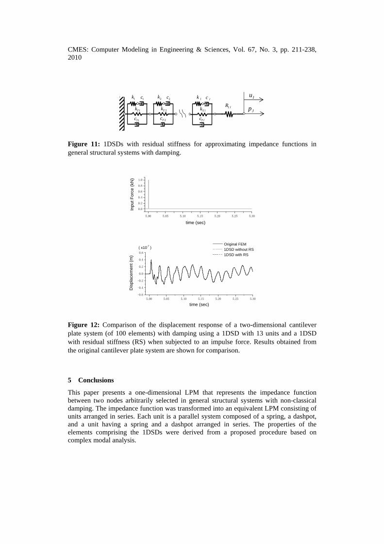
Figure 11: 1DSDs with residual stiffness for approximating impedance functions in general structural systems with damping.

5.00 5.05 5.10 5.15 5.20 5.25 5.30

0.0

0.2

0.4

0.6

0.8

1.0

time (sec)

Inpu

t For

ce (k

N)

5.00 5.05 5.10 5.15 5.20 5.25 5.30

-0.6

-0.4

-0.2

0.0

0.2

0.4

0.6

( x10-7 ) Original FEM 1DSD without RS 1DSD with RS

Dis

plac

emen

t (m

)

time (sec)

Figure 12: Comparison of the displacement response of a two-dimensional cantilever plate system (of 100 elements) with damping using a 1DSD with 13 units and a 1DSD with residual stiffness (RS) when subjected to an impulse force. Results obtained from the original cantilever plate system are shown for comparison.

5 Conclusions

This paper presents a one-dimensional LPM that represents the impedance function between two nodes arbitrarily selected in general structural systems with non-classical damping. The impedance function was transformed into an equivalent LPM consisting of units arranged in series. Each unit is a parallel system composed of a spring, a dashpot, and a unit having a spring and a dashpot arranged in series. The properties of the elements comprising the 1DSDs were derived from a proposed procedure based on complex modal analysis.


The applicability of the proposed transformation procedure and the accuracy of the impedance functions of the proposed 1DSDs were verified with three examples of structural systems. The results of the proposed transformation were compared with those evaluated directly from the original structural systems. In the transformation procedure, the number of elements and DOFs in 1DSDs could be reduced because of the symmetry in the shape and material properties of the structural systems. The results show that the impedance functions using the 1DSDs are in agreement with those evaluated from the original structural systems. A large number of units associated with high-order modes in the high-frequency region can be removed from the proposed 1DSDs as an approximate expression of impedance functions in a target frequency region. The accuracy of the approximated 1DSDs is improved by incorporating an additional unit associated with residual stiffness. This approximation can significantly reduce the DOFs of the 1DSDs, so a marked decrease in the computational domain size and time can be expected when solving dynamic problems.

References:

Andersen L. (2008): Assessment of lumped-parameter models for rigid footings. Computers and Structures (in press), available online. de Barros F. C. P.; Luco J. E. (1990: Discrete models for vertical vibrations of surface and embedded foundations. Earthquake Engineering and Structural Dynamics, 19, 289–303. Foss K. A. (1958): Co-ordinates which uncouple the equations of motion of damped linear dynamic systems. Journal of Applied Mechanics, 57, 361–364. Hizal N. A.; Gürgöze M. (1998): Lumped parameter representation of a longitudinally vibrating elastic rod viscously damped in-span. Journal of Sound and Vibration, 216(2), 328–336. Kolousek V. (1941): Anwendung des Gesetzes der virtuellen verschiebungen und des reziprozitatssatzes in der stabwerksdynamik. Ingenieur Archiv, 12, 363-370. Nagamatsu A. (1985): Modal Analysis. Baifukan, ISBN9784563034160 (in Japanese). Newmark J. K. (1959): A method of computation for structural dynamics. Journal of Engineering Mechanics Division, ASCE, 85, pp. 67–94. Saitoh M. (2007): Simple model of frequency-dependent impedance functions in soil-structure interaction using frequency-independent elements. Journal of Engineering Mechanics, ASCE, 133(10), 1101–1114. Weaver J. W.; Timoshenko S. P.; Young D. H. (1990): Vibration Problems in Engineering. Fifth Edition, Wiley Interscience. Wolf J. P. (1994): Foundation Vibration Analysis Using Simple Physical Models, Prentice-Hall, Englewood Cliffs, NJ. Wolf J. P. (1997): Spring-dashpot-mass models for foundation vibrations. Earthquake Engineering and Structural Dynamics, 26, 931–949. Wu W. H.; Lee W. H. (2002): Systematic lumped-parameter models for foundations based on polynomial-fraction approximation. Earthquake Engineering and Structural Dynamics, 31(8), 1383–1412.


Errata in the published article in CMES as follows: <Correct>

dnnn iωσλ +−= , (12)

dnnn iωσλ −−= , (13)

{ } [ ][ ][ ] [ ][ ][ ]( ){ }PU TT φγφφγφ += . (20)

ERRATA Masato Saitoh：Equivalent One-Dimensional Spring-Dashpot System Representing Impedance Functions of Structural Systems with Non-Classical Damping，CMES: Computer Modeling in Engineering & Sciences, Vol.67, No.3, pp.211-238, 2010. 11. Typographical errorta were discovered in Equation (12), (13) and (20). The corrected equations are as follows:

(Eq.12) dnnn iωσλ += ---> dnnn iωσλ +−=

(Eq.13) dnnn iωσλ −= ---> dnnn iωσλ −−=

(Eq.20) { } [ ][ ][ ] [ ][ ][ ]( ){ }PU TT φγφφγφ += ---> { } [ ][ ][ ] [ ][ ][ ]( ){ }PU TT φγφφγφ +=

.

Documents

Equivalent One-Dimensional Spring-Dashpot System ... Computer Modeling in Engineering & Sciences, Vol. 67, No. 3, pp. 211-238, 2010 Equivalent One-Dimensional Spring-Dashpot System