515

C H A P T E R

S e c t i o n 6

Prevention and Control of Infectious Diseases

61

Epidemiology of Equine Infectious DiseasePaulo C. Duarte, Ashley E. Hill, Paul S. Morley

Basics

Definition

Epidemiology is the study of the occurrence of disease in popu-lations1 and the application of this knowledge to control or prevent disease. The underlying tenet of epidemiology is that disease does not occur randomly in a population, which means that there are always reasons why some horses become sick and others stay healthy, even if we do not always understand those reasons. This principle has tremendous implications for veteri-narians: they can identify causes and risk factors for disease and take actions to prevent or decrease the impact of a disease. In this sense, it is critical to consider more than just disease agents and hosts; it is also critical to consider the environment and management factors that impact interactions among agents and hosts. Because of this broader implication, epidemiology is also sometimes defined as “medical ecology,” as will be discussed.

The mare reproductive loss syndrome (MRLS) outbreak in Kentucky in 2001 was an excellent example of epidemiology in action.2 Even before veterinarians and producers understood the etiology of this disease, veterinarians were able to use epi-demiology to identify risk factors for disease (exposure to eastern tent caterpillars2 or pasture3), which allowed farm man-agers to implement control measures and prevent some abor-tions that would have otherwise occurred.

Epidemiologic Approach

A key epidemiologic approach to understanding and controlling disease involves looking for patterns of disease in the popula-tion of interest. Which horses are sick, and what do they have in common? Which horses are healthy, and what do they have in common? Which groups have been most affected? Great insight can be gained into causal mechanisms and control points that can be exploited in disease prevention efforts by (1) describing a population and identifying patterns, (2) making comparisons among different groups within a population, (3) comparing different populations, and (4) comparing the same population at different time points.

It is useful to consider the “five Ws” when trying to under-stand disease occurrence in a population: who, what, where, when, and why. Who is affected (and unaffected)? Include age, breed, gender, housing, water source, and vaccination status, as well as any other variables that may be relevant. What are the circumstances related to disease occurrence and has anything changed? Where are the affected and unaffected animals located? Use a map of the barn or farm with food, water, and ventilation sources marked and spatially locate the ill animals. When did each ill animal develop disease? Use this information to identify groups most affected (e.g., age groups, barns, breeds) using the tools described later in this chapter. All of this should

be interpreted with a focus on ultimately identifying “why.” Why did these animals develop disease, and why were others not affected? Understanding why disease occurs allows identi-fication of ways that disease can be prevented.

Disease Ecology

When trying to understand reasons why particular animals become diseased, it is clearly important to consider more than just an individual host and a particular agent as causes for a specific occurrence. The population to which an individual belongs must also be considered, in addition to the patterns of interactions and the environment that influences these interac-tions and impacts the likelihood of contagious transmission. Because of the importance of these broader considerations, epidemiology is sometimes referred to as medical ecology, or the interactions of all organisms and their environment as these pertain to health.

Mare reproductive loss syndrome, which was initially reported among broodmares in central Kentucky in 2001, is one example of disease arising from a combination of host, agent, and environmental factors. An epidemic of equine abortion, endophthalmitis, and pericarditis began in late April 2001 and lasted until June 20014-6; fetal losses occurred both early and late in pregnancy3,7 and affected more than 60% of mares on some farms.7 Multiple bacterial species were identified8 in tissue of aborted fetuses. The syndrome was subsequently found to be associated with ingestion of the eastern tent caterpillar,4 and it has been proposed that bacterially contaminated barbed cater-pillar hairs migrated out of the alimentary tract, spread hema-togenously, and were directly responsible for the observable signs of MRLS.9 Eastern tent caterpillars are ubiquitous in the eastern United States but were particularly abundant in Ken-tucky that spring because a rapid temperature increase in early spring was superimposed on an unusually dry winter and spring.10 These climatic conditions caused an explosion of bio-logic activity, including growth of black cherry trees on which eastern tent caterpillar eggs are laid and larvae develop.11 During that spring with its unusual climactic conditions, grazing on pasture4 with black cherry trees12 exposed horses to disease; fetuses were particularly vulnerable. The sensitivity of the fetus to disease, the environmental conditions that led to the over-growth of caterpillars, the bacteria themselves, and the manage-ment of the broodmares all contributed to the occurrence of MRLS.

Disease AgentCharacteristics of the disease agent, including infectivity, con-tagiousness, pathogenicity and virulence, immunogenicity, host range, life cycle, and antimicrobial susceptibility, influence the speed and scope of disease spread. Infectiousness (infectivity) refers to the ease with which an agent infects susceptible hosts,

516 Section 6 Prevention and Control of Infectious Diseases

transport, or mixing, are more likely to develop a disease than their unstressed counterparts. The risk of disease is not equal for similar horses when managed differently or housed in dif-ferent environments.

IndividualEnvironmental characteristics that affect risk of disease in indi-vidual horses include climate, landscape, flora and fauna, cleanli-ness, air quality, housing, diet, and events that affect stress levels. Some of these factors (e.g., cleanliness, ventilation, housing, diet, stress level) are directly related to management practices and may be changeable, thus affecting risk of disease. Some management strategies (e.g., housing in open pastures, using outdoor drinking-water sources) increase potential exposure to insect vectors and also increase the risk of other diseases such as Potomac horse fever (Neorickettsia risticii infection) and vesicular stomatitis. On the other hand, indoor housing, espe-cially if it is high density or poorly ventilated, can increase exposure to diseases transmitted by aerosol or oral-fecal routes, such as influenza virus and Salmonella. Some environments and climates support larger vector populations than others, thus increasing potential risks for diseases, such as equine infectious anemia (EIA) or the equine encephalitides, including western equine encephalitis (WEE), eastern equine encephalitis (EEE), and WNV encephalitis. Although the climate itself cannot be changed, management practices, such as using animal-safe insect repellents, treating open-water sources with larvicides, and housing horses indoors at dusk and dawn, can be used to reduce disease risk.

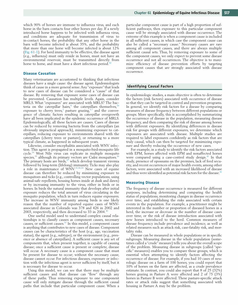
PopulationIn addition to characteristics of individuals that affect their disease risk, the aggregate characteristics of the population to which the individual belongs affects the disease risk for that individual. This aggregate of the population’s susceptibility to disease is often called herd immunity, described as immunity of an individual that is conferred by the population to which it belongs, or the ability of a population of animals to withstand exposure without succumbing to disease because the immunity of a population is more than the sum of its parts.31 Herd immu-nity is created when the likelihood is small that an infected horse shedding a disease agent will encounter a susceptible horse (Fig. 61-1). If most horses are immune or if contact among horses is heavily restricted, it is unlikely that the few susceptible horses will have contact with the infected horse sufficient to allow transmission. For example, consider a barn in

which is sometimes quantified in relation to the amount of agent required to reliably infect an individual. Contagiousness relates to the likelihood that an agent will move between infected and susceptible hosts; it is sometimes quantified by the number of new infections that will likely result from exposure to an infected animal or as the speed with which a disease agent is transmitted through a susceptible population. Equine influ-enza virus and equine herpesvirus are both highly infectious, but influenza virus is more contagious. Although equine proto-zoal myeloencephalitis (EPM) is an infectious disease, it is not a contagious disease because the etiologic agent is not transmit-ted directly between horses. Pathogenicity describes the likeli-hood that an infected horse will develop clinical disease, and virulence describes the likelihood that disease will be severe. West Nile virus (WNV) is highly virulent in horses; more than 30% of horses with clinical disease die.13 In contrast, EPM is not highly pathogenic; most equids exposed to the disease agent do not develop clinical disease.14-16

Characteristics of the disease agent that enable it to survive and spread without detection are particularly important to con-sider when instituting preventive or control measures. Agents that can persist in the environment, such as Clostridium diffi-cile17 or Streptococcus equi subsp. equi, require different control measures than equine influenza, which does not persist well outside the host. Some diseases spread undetected through infected horses without clinical signs of illness. Subclinically, persistently, and latently infected animals are often important reservoirs and sources of exposure for susceptible animals in a population because they go unnoticed or undiagnosed. Animals often are infected with a potentially pathogenic organism without showing clinical signs, and this can even be the pre-dominant presentation, depending on the pathogenicity of the agent. The term subclinical is also used to describe animals during the induction or incubation period for infectious dis-eases. Animals that remain infected for extended periods are sometimes described as being “persistently infected,” especially if infections continue after clinical signs of disease resolve. Per-sistent infection and long-term shedding of S. equi subsp. equi are common18-20 and important to the spread of disease among populations.20,21 In contrast, latency describes a state of dormant viral infection in which shedding stops and the virus cannot be detected until later, when the infection reactivates or recru-desces. This is a common feature among alpha herpesviruses such as equine herpesvirus (EHV) types 1 and 4.22-29

HostMany host characteristics are intrinsic to the horse and rela-tively unchangeable such as age, gender, and breed. Other host characteristics are highly variable among individuals and can change over time, perhaps most notably, an inherent suscepti-bility to infectious agents or immunity. Characteristics of the host can affect both its exposure to disease and its likelihood of becoming infected if exposed. For example, geldings or spayed mares are less likely to be exposed to Taylorella equigeni-talis, the agent that causes contagious equine metritis, and foals can be more vulnerable to disease than adults, as with Rhodococ-cus equi pneumonia.

EnvironmentA horse’s environment includes its location, climate, and the local surroundings and interactions created by its manage-ment.30 Characteristics of a horse’s environment affect which diseases and vectors a horse is exposed to, the magnitude of that exposure, and the likelihood of developing disease if exposed. Horses that have been vaccinated with efficacious vaccines or immunized by natural exposure are more resistant to a particu-lar disease than naïve horses. Horses that are stressed for any reason, including poor diet, concurrent disease, weaning,

Figure 61-1 Probability of new cases of disease with 1-day infectious period as a function of percentage vaccinated in a herd of horses where each horse contacts four other horses per day.

100%

90%

80%

70%

60%

50%

40%

30%

20%

10%

0%0% 20% 40%

Percent vaccinated

60% 80% 100%

Pro

babi

lity

of d

isea

se in

her

d

One new caseTwo new casesThree new cases

517Chapter 61 Epidemiology of Equine Infectious Disease

particular component cause is part of a high proportion of suf-ficient pathways, then exposure to this particular component cause will be strongly associated with disease occurrence. The extreme of this example is when a component cause is included in all sufficient causes, in which case the component cause can also be called a “necessary cause.” Necessary causes are rare among all component causes, and there are always multiple sufficient causal sets. Thus, by removing exposure to some of the component causes, we only expect to prevent some disease occurrence and not all occurrences. The objective is to maxi-mize efficiency of disease prevention efforts by targeting component causes that are strongly associated with disease occurrence.

Identifying Causal Factors

In epidemiologic studies, a main objective is often to determine the factors (risk factors) associated with occurrence of disease so that they can be targeted in control and prevention programs. In general, we identify risk factors for a disease by comparing measures of disease frequency between different populations or groups. More specifically, this is accomplished by summarizing the occurrence of disease in the population, measuring disease frequency, and then comparing the risk of disease among horses with different exposures. By identifying differences in disease risk for groups with different exposures, we determine which exposures are associated with disease. Multiple studies are required to label exposures confidently as risk factors that are truly causal, which can then be targeted for minimizing expo-sure and thereby reducing the occurrence of new cases.

For example, in a study to identify the risk factors associated with EPM, horses affected with EPM and nonaffected horses were compared using a case-control study design.41 In that study, presence of opossums on the premises, lack of feed secu-rity, and recent occurrences of major health events, among other factors, were associated with an increased likelihood of disease and thus were identified as potential risk factors for the disease.41

Measuring Disease

The frequency of disease occurrence is measured for different purposes, including determining and comparing the health status of populations, monitoring changes in disease occurrence over time, and establishing the risks associated with certain events in the population. For example, a practitioner might be interested in the number or proportion of diseased horses in a herd, the increase or decrease in the number of disease cases over time, or the risk of disease introduction associated with new horses introduced to the herd. Common measures of disease frequency include prevalence and incidence, as well as related measures such as attack risk, case-fatality risk, and mor-tality risks.

Disease can be measured in whole populations or in specific subgroups. Measuring disease in the whole population (some-times called a “crude” measure) tells you about the overall scope of the problem. Measuring disease in subgroups (called “spe-cific” measures) enables you to compare those groups, which is essential when attempting to identify factors affecting the occurrence of disease. For example, if you had 10 cases of neu-rologic disease on a farm of 100 horses, you could report that 10% of horses on the farm are affected, as a crude prevalence estimate. In contrast, you could also report that 8 of 25 (32%) horses grazing in Pasture A were affected and 2 of 75 (3%) horses in Pasture B were affected. These pasture-specific attack rates or attack risks suggest that something associated with housing in Pasture A may be the problem.

which 90% of horses are immune to influenza virus, and each horse in the barn contacts four other horses per day. If a newly introduced horse happens to be infected with influenza virus, and conditions are adequate for transmission of virus to in-contact horses, the probability that any other horse in the barn will become infected is about 35%, and the probability that more than one horse will become infected is about 12% (Fig. 61-1). For herd immunity to be effective, the disease agent (e.g., influenza) must only reside in horses, must not have an environmental reservoir, must be transmitted directly from horse to horse, and must have a short infectious period.32

Disease Causation

Many veterinarians are accustomed to thinking that infectious diseases have a single cause: the disease agent. Epidemiologists think of cause in a more general sense. Any “exposure” that leads to new cases of disease can be considered a “cause” of that disease. By removing that exposure some cases of disease can be prevented. Causation has multiple levels. Again, consider MRLS. What “exposures” are associated with MRLS? The bac-teria on the caterpillar hairs,8 the caterpillars themselves,33 exposure to cherry trees,2 pasture grazing,3,7 and the conver-gence of climatic factors resulting in caterpillar overgrowth have all been implicated in the epidemic occurrence of MRLS. Epidemiologically, all these factors are causes. Cases of disease can be reduced by removing bacteria from the caterpillars (an obviously impractical approach), minimizing exposure to cat-erpillars, reducing exposure to environments shared with the caterpillars (cherry trees or pasture), or returning to a more typical climate, as happened in subsequent years.

Likewise, consider encephalitis associated with WNV infec-tion. This agent is propagated in a mosquito-bird-mosquito life cycle.34 West Nile virus can replicate in multiple mosquito species,35 although its primary vectors are Culex mosquitoes.36 The primary hosts are birds,37 which develop transient viremia followed by long-term (lifelong) immunity. Ticks may also play a role in maintenance of WNV.35,38,39 New cases of equine disease can therefore be reduced by minimizing exposure to mosquitoes and ticks (e.g., controlling vector populations, using animal-safe repellents, housing horses inside at dusk and dawn) or by increasing immunity to the virus, either in birds or in horses. In birds the natural immunity that develops after initial exposure reduces the total amount of virus circulating in the mosquito population, which in turn reduces equine exposures. The increase in WNV immunity among birds is one likely reason that the number of reported equine cases of WNV-associated disease in Colorado was 378 and 426 in 2002 and 2003, respectively, and then decreased to 33 in 2004.40

One useful model used to understand complex causal rela-tionships is to classify causes as component causes, necessary causes, or sufficient causes.31 In this model, a component cause is anything that contributes to new cases of disease. Component causes can be characteristics of the host (e.g., age, vaccination status), the agent (e.g., subtype), or the environment (e.g., pres-ence or absence of caterpillars). A sufficient cause is any set of components that, when present together, is capable of causing disease; once a sufficient cause is present or complete, disease will occur. A necessary cause is a component cause that must be present for disease to occur; without the necessary cause, disease cannot occur. For infectious diseases, exposure or infec-tion with the infectious agent is never sufficient by itself, but it is necessary for disease to occur.

Using this model, we can see that there may be multiple sufficient causes and that disease can “flow” through any of these paths. Thus removing exposure to one component cause will only mitigate disease through the sufficient causal paths that include that particular component cause. When a

518 Section 6 Prevention and Control of Infectious Diseases

with the 25th and 75th percentiles), or the standard deviation or standard error of the mean. A simple arithmetic average summarizes the data well if the distribution of values looks like the well-recognized “normal” or “bell-shaped” curve. However, in distributions that do not have this balanced shape or in situ-ations in which there are relatively few observations, averages can be strongly influenced by extreme values and may not represent the “center” of the data very well. In these situations, the median or mode will likely provide better measures of centrality in the data.

Using Categorical DataRatios, Proportions, and RatesWhen using ratios, proportions, and rates to summarize disease occurrence, a count of affected animals meeting a specific case definition is used as the numerator. Do 10 affected horses rep-resent a significant number of cases? The answer depends on the type of disease and the size of the population in which these observations were made. Are we referring to 10 sick horses in a barn of 15 horses or 10 sick horses at an entire racetrack facil-ity with 3500 horses? The denominator provides context (e.g., is the population-at-risk 15 or 3500 horses) and improves standardization and the ability to extrapolate or make compari-sons. The type of denominator we choose affects the conclu-sions we can draw. The ratios, proportions, and rates used as epidemiologic measures principally differ in how the denomi-nator is calculated (e.g., which animals are included, is time considered).

RatiosRatios are used to express the magnitude of two events in relation to each other. Ratios vary between 0 and infinity and can also be expressed as the number of events in one group per number of events in another group. In a ratio, the numer-ator is not part of the denominator. For example, in a popula-tion of horses, a ratio of infectious upper respiratory tract disease (IURD) of 0.25, or 1 : 4, indicates that there is one dis-eased for every four nondiseased horses. In this case, we can also say that the odds of IURD in the population is 1 : 4. Ratios are also used to compare measures of disease frequency between groups.

ProportionsA proportion is a special type of ratio in which the numerator is included as part of the denominator. For disease measure-ment, this fraction is calculated as the number of events over the total number of possible events. A proportion varies between 0 and 1 and is usually expressed as percentage. For example, during a regular clinical examination, 10 of 100 horses exam-ined were identified with IURD. The proportion of IURD among these 100 horses at the time of examination was 10/100, or 10%. In another situation, 100 horses were followed for 1 year. During that year, 20 new cases of IURD were identified. The proportion of new IURD cases during that 1-year period was 20/100, or 20%.

RatesA rate is another special type of ratio. In epidemiologic terms, rate represents the average “speed” that health events will occur in a population over a specific or standardized amount of time. A rate is calculated as the number of events over the product between the total number of possible events and the time period during which each event could have occurred. A rate varies between 0 and infinity, and the units of the denominator are expressed in event-time (e.g., horse-years, horse-months). For example, 100 horses were followed for 1 year. Assume that 10 horses developed IURD in the middle of the year (0.5 year)

Population-at-RiskThe term population-at-risk refers to the group of individuals susceptible to the event of interest (e.g., infection, disease, death) at or during the time period of interest. The population-at-risk is used as the denominator in calculations of measures of disease frequency and can include the entire population or only a population subset, depending on susceptibility or specific interest in certain subgroups. For example, in describing the frequency of pneumonia caused by Rhodococcus equi infections, only foals would likely be included in the population-at-risk because adult horses are not considered susceptible to this disease.42

Types of DataThe types of data available largely determine which methods will be most appropriate for measuring disease frequency or comparing disease risk. Most data can be described as interval (measurement) or categorical data. Interval data quantify a characteristic, such as temperature, age, or weight, which can measure a large range of possible values. For example, in a group of five horses, you might take temperature measurements of 100° F, 100° F, 101° F, 101.5° F, and 102° F. Average or median values are often used to summarize interval data, and for this example, the average temperature for these five horses is 100.9° F. Interval data are often compared by subtracting one average or median from another, and differences in interval measurements among groups are often statistically tested using z-tests, t-tests, analyses of variance (ANOVA), or linear regression.

Categorical data divide groups into mutually exclusive cat-egories (e.g., young horses versus older horses, Quarter Horses versus Thoroughbreds), and counts are used to characterize horses fitting into each category. Categorical data can be further characterized as “ordinal” if categories have an inherent order to them (e.g., young or old, light or heavy) or “nominal” if cat-egories cannot be ranked or ordered (e.g., categories for gender or breed). Interval measurements can also be converted to ordinal measurements by dividing your range of values into categories. For example, if you wanted to describe temperature ordinally, as <101.5° F (38.6° C) versus temperature ≥101.5° F for these five horses, you would report that three horses had temperatures <101.5° F, and two had temperatures ≥101.5° F. Categories for nominal or ordinal data can be dichotomous (only two values are possible [e.g., live/dead, yes/no, sick/well]) or can have more than two possible values (e.g., breed, age group). Ordinal and nominal data are summarized using ratios, proportions, and rates. These summary measurements can then be compared using relative risks (risk ratios), odds ratios, and attributable risks. These comparisons are often tested statisti-cally using different types of chi-square tests or logistic regres-sion if the outcome data are dichotomous.

Generally, all characterizations of disease occurrence in pop-ulations include some type of categorical assessment of pres-ence or absence of disease signs using a specific case definition. In summarizing these measurements, the data are standardized to account for population sizes using the number of affected animals as a numerator, and some context measurement of the “opportunity” for disease to have occurred in the population (e.g., the population at risk). The denominator that we choose greatly affects the conclusions we can draw from these measure-ments of disease frequency. In general, these measures of disease frequency take the form of ratios, proportions, or rates.

Using Interval DataInterval data are usually summarized using a measure that describes central tendency (e.g., means, medians, or modes) and some measure of the variability in data such as the range of observed values, percentile rankings (e.g., values corresponding

519Chapter 61 Epidemiology of Equine Infectious Disease

The cumulative incidence is an appropriate measure of disease incidence when the population is relatively “closed” (i.e., minimal movement of animals in and out of the population). When there is substantial movement of animals (“open” popula-tion), the cumulative incidence might underestimate or over-estimate (bias) disease incidence,43 and the incidence rate, also called incidence density, is a more appropriate measure of disease incidence.

Other common measures that could be described as specific types of cumulative incidence include the attack rate, mortality rate, and the case-fatality rate. The attack rate or attack risk is simply a different name attributed to the cumulative incidence in an outbreak situation and is calculated exactly as the cumula-tive incidence. The mortality rate or mortality risk is the propor-tion of all deaths (“crude” mortality rate) or deaths attributable to a specific disease (“cause-specific” mortality rate) over the total population-at-risk of death at the beginning of the time period (Box 61-3). Note that these measures are often called “rates,” but in reality they are proportions because they do not include time measurements in their denominator and thus it is more precise to call them “risks.”

Mortality can be calculated as a proportion, as just noted, or as an incidence using one of the methods described next. The term mortality rate is commonly used to describe mortality in the population, whether it is a proportion (risk) or an actual rate.

The case-fatality rate is the proportion of deaths attributable to the disease of interest during a specific period of time (Box 61-4).43 The case-fatality rate is calculated as follows:

and after this point were no longer at risk of IURD because of acquired immunity. The rate of IURD would be calculated as 10 cases/[(90 horses × 1 year) + (10 horses × 0.5 year)] and expressed as 0.11 cases per horse-year, or 11 cases per 100 horse-years. Notice that the time units of the denominator can be changed as desired, and 11 cases per 100 horse-years is the same as 11 cases per 1200 (100 × 12) horse-months, which means that you expect approximately 11 cases of IURD if you follow 100 horses for 1 year or 1200 horses for 1 month. Simi-larly, 33 cases of IURD would be expected to occur if 100 horses were followed for 3 years. The word “rate” is commonly used to refer to a proportion; however, rates and proportions are different quantities and are calculated differently, even though they are sometimes used as approximations of each other.

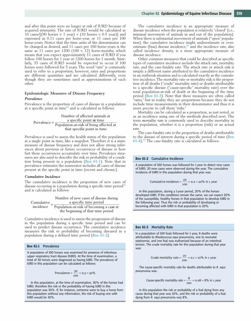
Epidemiologic Measures of Disease FrequencyPrevalencePrevalence is the proportion of cases of disease in a population at a specific point in time43 and is calculated as follows:

Prevalence

Number of affected animals ata specific point i= nn time

Population-at-risk of being affected atthat specificc point in time

Prevalence is used to assess the health status of the population at a single point in time, like a snapshot. Therefore it is a static measure of disease frequency and does not allow strong infer-ences about previous or future occurrences of disease or how fast these occurrences accumulate over time. Prevalence mea-sures are also used to describe the risk or probability of a condi-tion being present in a population (Box 61-1). Note that in prevalence estimates the numerator includes all cases of disease present at the specific point in time (recent and chronic).

Cumulative IncidenceThe cumulative incidence is the proportion of new cases of disease occurring in a population during a specific time period43 and is calculated as follows:

Cumulativeincidence

Number of new cases of disease duringa= specific time period

Population-at-risk of becoming a casee atthe beginning of that time period

Cumulative incidence is used to assess the progression of disease in the population during a specific time period and can be used to predict disease occurrence. The cumulative incidence measures the risk or probability of becoming diseased in a population during a defined time period (Box 61-2).

Box 61-2 Cumulative Incidence

A population of 100 horses was followed for 1 year to detect new cases of IURD; 20 new cases were observed during the year. The cumulative incidence of IURD in this population during that year was:

Cumulative incidence in year= = =20100

0 2 20 1. %

In this population, during a 1-year period, 20% of the horses developed IURD. If the conditions remain the same, we can expect 20% of the susceptible, healthy horses in that population to develop IURD in the following year. Thus the risk or probability of developing or becoming affected with IURD in that population is 20%.

Box 61-1 Prevalence

A population of 100 horses was examined for presence of infectious upper respiratory tract disease (IURD). At the time of examination, a total of 30 horses were diagnosed as having IURD. The prevalence of IURD in this population can be calculated as follows:

Prevalence = = =30100

0 3 30. %

In this population, at the time of examination, 30% of the horses had IURD; therefore the risk or the probability of having IURD in this population was 30%. If, for instance, someone were to buy a horse from this population without any information, the risk of buying one with IURD would be 30%.

Box 61-3 Mortality Rate

In a population of 100 foals followed for 1 year, 8 deaths were attributable to Rhodococcus equi pneumonia, one to neonatal septicemia, and one foal was euthanized because of an intestinal torsion. The crude mortality rate for this population during that year was:

Crude mortality rate 1 in year= = =0100

0 1 10 1. %

The cause-specific mortality rate for deaths attributable to R. equi pneumonia was:

Cause-specific mortality rate 8 in year= = =100

0 08 8 1. %

In this population the risk or probability of a foal dying from any cause during that year was 10%, and the risk or probability of a foal dying from R. equi pneumonia was 8%.

520 Section 6 Prevention and Control of Infectious Diseases

risk of developing IURD in this population in 1 year, although this is a less precise interpretation.

Two other approximations can be used to estimate the denominator incidence rates when information on disease-free time for each individual horse is not available: (1) average the population-at-risk at the beginning and at the end of the time period of interest or (2) use an estimate of the total population at a certain point in time during the period of interest (usually the middle of the time period) as the average population-at-risk. In both cases, we assume that the average population represents the average number of horses at risk for a period of time equiva-lent to the follow-up period, and we calculate the incidence rate denominator as the product between the average population-at-risk and the follow-up period.

In these examples, we assumed that once a horse developed IURD, it also developed immunity to the disease, and thus there were no recurrences during that year. To account for recurrences, the total number of occurrences per horse would be included in the numerator, with the total disease-free time between occurrences for each horse included in the denominator.

Relationship between Prevalence and IncidencePrevalence of disease is a function of disease incidence and duration.43 In general, prevalence increases as the incidence and duration of disease increase, and vice versa (Box 61-6). This relationship can be used for approximation of incidence or prevalence if one measure or the other is available.

Temporal Patterns of Disease

Characterizing and understanding the occurrence of disease over time in populations are very useful and can provide great insight into the infectivity and contagiousness of disease. One standard method of graphically summarizing disease temporally is to generate an epidemic curve by plotting the number of new

Box 61-5 Incidence Rate

A total of 100 horses were followed for 1 year. During the year, there were 20 new cases of IURD, all of which occurred in the third month of the year (0.25 year). In addition, 10 horses were sold and left the population at 6 months (0.5 year) into the year, and another 5 horses died of other causes. Among these five horses, one died at 2 months (0.2 year) into the year, two at 4 months (0.3 year), and the other two at 9 months (0.75 year) into the year. The incidence rate was:

Incidence rate

=× + × + × + × + × +

2065 1 10 0 5 1 0 2 2 0 3 2 0 75( ) ( . ) ( . ) ( . ) ( . ) (220 0 2520

77 3

×

=

. )

.

Incidence rate ≅ 0.26 cases/horse-years or 26 cases/100 horse-yearsExplanation of the calculations in the denominator:65 × 01 = Time-at-risk accumulated by horses that never developed

IURD and were at risk for the disease for the entire 1 year (disease-free time).

10 × 0.5 = Time-at-risk accumulated by horses that left the population in the middle of the year and thus were at risk for IURD for 0.5 year each.

(1 × 0.2), (2 × 0.3), and (2 × 0.75) = Time-at-risk accumulated by horses that died of other causes and were at risk of IURD during the time they were alive: 0.2 year for one horse, 0.3 year for two horses, and 0.75 year for two horses.

20 × 0.25 = Time-at-risk accumulated by horses that developed IURD at 3 months into the year and were at risk for the disease for 0.25 year each.

Box 61-4 Case-Fatality Rate

A population of 100 foals was followed for 1 year. During that period, there were 20 new cases of R. equi pneumonia identified. Ten of the 20 affected foals died as consequence of the disease during the year. The case-fatality rate for R. equi pneumonia in that population of foals during that year was:

Case-fatality rate in year= = =1020

0 5 50 1. %

In this population, once a foal is affected by R. equi pneumonia, the risk or probability of dying from the disease is 50%.

Case-fatality rate

Number of deaths attributable to thedis= eease during a specific time period

Total number of cases off diseasein that time period

This measure of disease occurrence is often used to characterize the severity of disease and the effectiveness of treatment. Therefore the specific case-fatality rates for treated and untreated animals are often cited and compared.

Mortality rates and case-fatality rates are two of the most frequently confused epidemiologic measures, and they actually describe very different disease characteristics. Mortality rates are used to describe the risk or probability of death in a popula-tion (whether estimated by prevalence, cumulative incidence, or incidence density). This can be death attributable to all causes or death associated with a specific condition. In contrast, the case-fatality rate characterizes the likelihood of death once a condition is present. As such, the cause-specific mortality rate can be very low for a given disease, whereas the treated or untreated case-fatality rate for the same disease can be very high. For example, the mortality rate for rabies is very, very low among horses in most parts of the world. This means that very few deaths are associated with this disease in most equine populations. However, both the treated and untreated case-fatality rate is essentially 100% for rabies. This means that all horses which develop rabies can be expected to die.

Incidence RateThe incidence rate is the number of new cases of disease per unit of animal-time. There are different ways to calculate inci-dence rate depending on the information available. The most accurate is as follows:

Incidence rate

Number of new cases of diseasein a specific= time period

Sum of each individual s disease-free timein

’tthe population-at-risk

in the specific time period

The incidence rate, as the cumulative incidence, is used to assess the progression of disease in the population and can be used to predict disease occurrence. It is calculated for a specific time period, but it represents a measure of the “speed” of the disease in the population over time. In practice, incidence rate and cumulative incidence are used as approximations of each other and are given the same interpretation. The type of the popula-tion (open or closed) and the data available are what determines which is calculated. The incidence rate is not a true measure of risk but can be and is used as such (Box 61-5).

In the example in Box 61-5, we can say that, if everything remains constant, the disease is “moving” through the popula-tion at an average “speed” of 26 cases per 100 horses per year. For practical purposes, we might also say that there is a 26%

521Chapter 61 Epidemiology of Equine Infectious Disease

occurrences that develop per units of time (time is traditionally graphed on the x axis in whatever intervals make sense; case frequency is plotted on the y axis; Fig. 61-2). In general, the occurrence of disease over time can be grouped into four cat-egories: endemic, epidemic, pandemic, and sporadic.30

A disease is endemic (Fig. 61-2, A) if it occurs at some pre-dictable rate regardless of whether that rate is high, low, or varies during a given year or other specific time period. For example, in some regions of the United States, Potomac horse fever (PHF) is endemic because the number of new cases is relatively constant from year to year. Salmonellosis is also endemic throughout the United States, although the rates pre-dictably increase in the summer and early fall.

A disease is epidemic (Fig. 61-2, B) when it occurs at a level beyond that which is typical or expected in the population.30 For example, introduction of WNV into the United States created epidemics in horse populations throughout North America.13,44-50 Strangles is endemic in the United States as a whole but often occurs as outbreaks or epidemics at the local level. When epidemics affect populations across multiple con-tinents, then disease is sometimes considered pandemic (e.g., H5N1 avian influenza in 2003–2005,51 “type 2” (H3N8) equine influenza in 196352-55) (Fig. 61-2, C). Epidemics and pandemics occur when a highly contagious disease is introduced into a susceptible population.

A disease is considered sporadic (Fig. 61-2, D) if it occurs irregularly and haphazardly; sporadic disease can occur as a single case or as a cluster of cases. Vesicular stomatitis occurs sporadically in horses in the western United States.56-58 Sporadic disease can be the result of infrequent contact between a sus-ceptible animal and a reservoir of disease.

From a conceptual perspective, epidemics can be further separated into two general patterns: point-source and propa-gated (Fig. 61-3). A point-source epidemic occurs when many horses in a population are exposed at the same time to a specific disease agent. For example, a point-source epidemic might occur if a group of horses are all exposed at the same time to a toxin in the feed, such as mycotoxin-contaminated ryegrass hay.59 An epidemic curve of a point-source outbreak (Fig. 61-3, A) shows a high number of initial cases, but the number of new cases often taper off quickly when the exposure to the agent is removed or disappears. Propagated epidemics occur when an infectious agent, equine influenza virus,60 is spread from one or a few initially infected horses (“primary” cases) to other suscep-tible horses (“secondary” cases) that spread disease themselves (Fig. 61-3, B). For propagated epidemics of contagious disease, the number of new cases classically increases exponentially over days to weeks as susceptible horses become infected, then tapers off gradually as the number of susceptible horses in the population decreases and concomitantly, exposures decrease.

This conceptual model of different epidemics is very useful, but differentiating between point-source and propagated out-breaks is not always easy based on the shape of their epidemic curves. For example, a group of horses could all develop salmo-nellosis after consuming contaminated feed; the horses may then shed Salmonella in their feces, thus infecting other horses

Figure 61-2 Epidemic curves associated with A, endemic disease (Potomac horse fever); B, epidemic disease (equine West Nile encephalitis cases in California70); C, pandemic disease (H5N1 avian influenza in Asia 2003–200551); and D, sporadic disease (vesicular stomatitis in western United States57,58,71-73).

250

200

150

No.

new

cas

es

100

50

0

Month

Jan

Feb

Mar

Apr

May Jun

Jul

Aug

Sep Oct

Nov

Dec

No.

infe

cted

pre

mis

es

600

500

400

300

200

100

0

Year

1986

1990

1994

1998

2000

No.

new

cas

es (

x100

0)

100,000

10,000

1000

100

10

0

Month

Jan

Feb

Mar

Apr

May Jun

Jul

Aug

Sep Oct

Nov

Dec Jan

Dec

201816141210

No.

new

cas

es

1996

1997

1998

1999

2000

2001

2002

2003

2004

86420

YearA

B

C

D

Box 61-6 Prevalence and Incidence

In Box 61-2 the cumulative incidence of IURD was 20%. Assume average disease duration of 7 days (or 0.02 year). The prevalence of IURD at any given day of the year is approximately:

Prevalence Cumulative incidence DurationCumulative incide

≅ ×( nnce Duration× +

= ×× +

=)

. .( . . )

. %1

0 20 0 020 20 0 02 1

0 4

522 Section 6 Prevention and Control of Infectious Diseases

and consider the p value. The p value indicates the statistical significance of the association, or how likely we are to see results this extreme if no association existed between the factor and the disease.62 A p value of <0.01 suggests that if there truly were no causal association between fever and Salmonella shedding, we would still see an odds ratio of 9.0 in a similar study less than 1% of the time. In other words, it is likely that the associa-tion is real, not just coincidence. The p value is greatly affected by the number of horses in the study (i.e., study power), the magnitude of the difference being measured (i.e., strength of association), and the degree of variation in the groups being compared (did all febrile horses and none of the afebrile horses shed Salmonella, or was there more variation in shedding within febrile and afebrile groups?). In general, the p value decreases as the number of animals being studied increases, as the mag-nitude of difference increases, and as the variation within each group decreases. The p value does not provide any information about whether the difference between groups is meaningful.

Using Measurement DataIs the Difference Real?If data follow a bell-shaped curve, the z-test or t-test can be used to determine how likely it is that the difference is real and not caused by chance variation. Many basic statistical packages (e.g., http://wwwn.cdc.gov/epiinfo/) will perform these simple statistical tests, or you can even use online calculators (e.g., http://www.vassarstats.net/tu.html). You can also perform this simple calculation by hand. To calculate the z-test by hand, the standard deviation (SD) of each group’s data (a $5 calculator can do this for you), the number (count) of horses in each group, and the z-score values for different “confidence” levels (95% = 1.96; 90% = 1.64; 80% = 1.28) must be known. The following formula is used to calculate the limits for a confidence interval, using the 95% z-score of 1.96:

Average Average z-scoreSD

countSD

count1 2

11

22

2 2

− ± × +

If the range estimated by this calculation does not include zero, there is 95% confidence that the observed difference is real and not caused by chance. If the range does include zero, the equa-tion is recalculated using the 90% z-score of 1.64. If the new range does not include zero, there is 90% confidence that the difference is real. If the 90% range includes zero, the equation is recalculated using the 80% z-score. If the range does not include zero, there is 80% confidence that the difference is real; if the range does include zero, there is less than 80% confidence that the difference is real.

For example, if there was a concern that poor ventilation in Barn A was affecting the horses, rectal temperature data for 10 horses in Barn A and 15 horses in Barn B could be collected. If the average temperature of horses in Barn A was 102.0° F (38.8° C) with SD of 0.56, compared with 100.6° F (38.1° C) with SD of 0.71 for horses in Barn B, the limits for a 95% confidence interval for the average difference could be calcu-lated using the following equation:

102 0 100 6 1 960 56

100 71

151 4 0 50 0 9 1 9

2 2

. . .. .

. . . , .− ± × +

= ± =

The 95% confidence interval for the difference of these average rectal temperatures is 0.9 to 1.9, which does not include zero, so there is 95% confidence that the difference is real and not caused by chance variation. Is an average body temperature difference of 1.4° F biologically meaningful? That cannot be

in their paddocks. Although the disease outbreak originated from a single source, it was then propagated through fecal-oral transmission. The shape and time scale of a propagated epi-demic curve are affected by the disease incubation period, how contagious the disease is, what proportion of horses in the herd are susceptible, and how densely the horses are housed.30

Comparing Groups

There are two important questions to answer when comparing data from two or more groups. First, how “big” is the difference between groups? One way of evaluating how “big” is “big” is to consider whether the difference seems biologically or economi-cally meaningful. The second question that must be considered is whether the observed difference is “real,” or could it be caused more by chance variation than by a systematic difference? To quantify the size of differences between groups, typically a summary measure, such as averages or proportions, is compared or a measure of association, such as an odds ratio or relative risk, is calculated. Using this comparative information, it is necessary to evaluate whether the observed differences are meaningful or trivial. For example, in a study evaluating Salmo-nella shedding among colic patients, the association between having a fever and shedding Salmonella was reported61 as an odds ratio of 9.0 with a p value of <0.01, indicating that horses shedding Salmonella were about nine times more likely to have a fever than horses not shedding Salmonella. This seems like a meaningful difference (i.e., nine times more likely is biologically meaningful), and the p value suggests that this difference is unlikely to have occurred from chance alone.

To evaluate whether there is a “real” difference versus a dif-ference that occurred from chance variation, we typically use some type of statistical evaluation (e.g., chi-square test, z-test)

Figure 61-3 Epidemic curves from point-source outbreak of neurologic signs associated with A, consumption of mycotoxin-contaminated ryegrass,59 and B, propagated outbreak of infectious upper respiratory disease.60

12N

o. n

ew c

ases

10

8

6

4

2

0

17-J

an

21-J

an

25-J

an

29-J

an

2-F

eb

6-F

eb

10-F

eb

14-F

eb

Date

12

No.

new

cas

es

10

8

6

4

2

0

28-J

un

2-Ju

l

6-Ju

l

10-J

ul

14-J

ul

18-J

ul

22-J

ul

26-J

ul

Date

A

B

523Chapter 61 Epidemiology of Equine Infectious Disease

group. It measures how large the odds of disease are in the exposed group compared with the nonexposed group. Fre-quently, diseased and nondiseased horses are the groups selected in epidemiologic studies, and differences in exposure between groups are determined. In these cases, strictly speaking, the OR is the ratio between the odds of exposure in the diseased group over the odds of exposure in the nondiseased group. However, mathematically, the OR calculated as the odds of exposure in the diseased and nondiseased groups and the odds of disease in the exposed and nonexposed groups are the same (Box 61-10).

The RR and OR are also called “measures of strength of association” as they are not only indicators of whether an asso-ciation exists, but also the direction and strength of the associa-tion. An RR or OR of 5 indicates a much stronger association between the risk factor and the disease than an RR or OR of 1.5. An RR or OR equal to 1 indicates no association between the risk factor and the disease. In other words, it indicates that disease is as likely to occur in the exposed as the nonexposed group. An RR or OR less than 1 indicates that the risk factor is actually protective for the disease and technically is not a risk but a protective factor. A common example is vaccination. An RR or OR of 0.5 obtained when comparing occurrence of disease in vaccinated (exposed) and nonvaccinated (nonex-posed) horses indicates that disease occurrence in vaccinated horses is about half of that in nonvaccinated horses.

Outbreak Investigations: Attack Risk TableAn attack risk (attack rate) table is a quick and simple way to summarize exposures and disease occurrence and also to look for factors strongly associated with disease. It is often used to analyze data quickly during an outbreak. Consider a farm on which 10 cases of strangles are diagnosed in a population of 100

determined by a statistical test and is better determined using clinical experience and judgment.

Using Categorical DataIn epidemiology, it is common to use the term exposure to refer to an individual’s experience with a risk factor. In a study of EPM occurrence, lack of feed security was identified as a poten-tial risk factor for the disease.41 Horses “exposed” to “lack of feed security” were more likely to have EPM than horses “not exposed” to “lack of feed security” (i.e., horses that had their feed safely stored). Thus it is important to notice that “expo-sure” is used broadly in epidemiology and does not necessarily refer to the physical contact between the risk factor and the individual, as it might initially suggest.

Various measures of association can be used to characterize relationships between risk factors and disease. The timing of data collection relative to disease occurrence dictates to a great extent which measures of association are appropriate. If horses exposed and not exposed to a potential risk factor are followed over time to determine occurrence of disease (cohort studies), measures of incidence are obtained, and measures of association (e.g., attributable risk, attributable fraction, relative risk, odds ratio) can all be estimated. If diseased and nondiseased horses are compared in relation to their past or current exposure to a potential risk factor (case-control and cross-sectional studies), the odds ratio is the measure of association estimated.

Comparing Cumulative Incidence: Attributable Risk and Attributable FractionThe attributable risk (AR) estimates the absolute amount of risk that is conferred or attributed to exposure in the group of individuals with the risk factor. The AR is calculated as the dif-ference between the cumulative incidence in horses exposed and not exposed to the risk factor. Similarly, the attributable fraction (AF) is the proportion of risk attributable to exposure to the risk factor and is calculated as the AR divided by the cumulative incidence in the exposed group (Box 61-7).

In Box 61-7, 50% (10% of 20%) of the risk of IURD in horses housed in poor bedding conditions is attributable to the actual exposure to poor bedding conditions. In other words, if you could transfer all horses in poor bedding conditions to good bedding conditions, you might expect that this would prevent 50% of disease in that group. In the population there is a mixture of horses exposed and not exposed to poor bedding conditions. Therefore the reduction in disease occurrence in the population as a whole (not only in the exposed group) will depend on the proportion or prevalence of exposure in that population.

To determine the impact of control and preventive measures in the population, two other measures can be calculated: the population AR and the population AF. The population AR mea-sures the amount of risk attributable to exposure in the popula-tion and is calculated as the product of the AR and the prevalence of exposure in the population.43 The population AF is the proportion of risk attributable to exposure in the popula-tion and is calculated as the population AR divided by the cumulative incidence of the disease in the entire population (CITP) (Box 61-8).43

Comparing Cumulative Incidence: Relative RiskThe relative risk or risk ratio (RR) is the ratio between the cumulative incidence or disease risk in the exposed and nonex-posed groups. It measures how large the cumulative incidence is in the exposed group compared with the nonexposed group (Box 61-9).

Comparing Prevalences: Odds RatioThe odds ratio (OR) is the ratio between the odds of disease in the exposed group and the odds of disease in the nonexposed

Box 61-7 Attributable Risk

Assume that veterinarians at a racetrack believe that housing conditions contribute to the risk of IURD occurrence and that exposure to dusty environments with high levels of ammonia increase the likelihood of IURD occurrence. In other words, they believe that poor bedding (PB) conditions serve as a risk factor for IURD. A cohort study was designed to determine whether there was an association between PB conditions and occurrence of IURD. A sample of 100 horses housed in PB conditions and another sample of 100 horses housed in good bedding (GB) conditions were followed for 1 year. The cumulative incidence (CI) was calculated for both groups and compared. The data are presented below:

CIPB CIGB= = = =20100

20 10100

10% %

Attributable risk CIPB CIGB= − = − =20 10 10% % %

Attributable fraction CIPB CIGBCIPB

= − = − =20 1020

50% %%

%

In this example, the attributable risk indicates that 10% of the 20% total risk of IURD in horses exposed to poor bedding conditions was actually attributable to the horses being housed in poor bedding conditions. The attributable fraction indicates that this 10% of the risk represented 50% of the total risk of IURD in the horses exposed to poor bedding conditions. Note that IURD also occurred in horses housed in good bedding conditions. Therefore, poor bedding conditions contribute to an increase in IURD but are not the only factor associated with its occurrence.

Poor Bedding

Good Bedding

IURD+ 20 10 30IURD− 80 90 170

100 100

524 Section 6 Prevention and Control of Infectious Diseases

Box 61-8 Attributable Fraction

Based on the information obtained in the study described in Box 61-7, the veterinarians at the racetrack decided to implement a program to improve bedding conditions in the entire racetrack (the population). They want to know the impact such a program will have in reducing IURD in the population. According to a previous survey conducted at the racetrack, approximately 30% of the horses were housed in poor bedding conditions (exposure prevalence). Using the data from Box 61-7, the population attributable risk (PAR) and the population attributable fraction (PAF) were:

Population attributable risk Exposure prevalence= × = ×AR 10 30% %% %= 3

Population attributable fraction = = =PARCITP

313

23%%

%

Where:CITP = Cumulative incidence of IURD in the entire populationCITP = (CIPB × exposure prevalence) + {CIGB × (1 − exposure prevalence)}CITP = (20% × 30%) + (10% × 70%) = 13%By implementing a program to improve bedding conditions at the racetrack, practitioners may expect an absolute reduction of 3% in the total IURD

incidence. This reduction represents approximately 23% of the total current incidence of IURD (13%) at the racetrack. In other words, the veterinarians might expect to reduce the total incidence of IURD at the racetrack from 13% to 10%. The PAR and the PAF can also be calculated as:

Population attributable risk CI CITP GB= −

Population attributable fraction CI CICI

TP GB

TP= −

Where:CITP = Cumulative incidence of IURD in the entire populationCIGB = Cumulative incidence of IURD in the nonexposed (good bedding) horses

Box 61-10 Odds Ratio

A study was conducted to evaluate risk factors associated with development of equine protozoal myeloencephalitis (EPM). Using a case-control study design, horses with EPM were identified for enrollment. “Security” of the hay fed to the horses from wildlife was evaluated as one of the potential risk factors.41 Horses fed hay from “nonsecure” sources were considered “exposed,” whereas horses fed hay that was protected from exposure to definitive hoses (secure hay) were considered “nonexposed.”

Calculations for the odds ratio for EPM occurrence in the exposed and nonexposed groups is shown below:

Odds ratio = ××

≅86 4851 43

2

An odds ratio of 2 indicates that horses exposed to nonsecure hay were approximately two times more likely to develop EPM than horses fed secure hay. Note that the interpretation of the odds ratio is similar to the interpretation of the relative risk (see Box 61-9), even though measures of disease incidence were not calculated. In epidemiologic studies the odds ratio is used as an approximation of the relative risk when the study design does not allow the calculation of measures of incidence. This approximation is more precise when the disease is rare in the population.30

EPM+ EPM−Hay not secured

86 51 137

Secured hay

43 48 91

129 99 228

Box 61-9 Relative Risk

As in Box 61-7, a cohort study was designed to determine whether there was an association between poor bedding conditions and occurrence of IURD. A sample of 100 horses housed in poor bedding conditions and another sample of 100 housed in good bedding conditions were followed for 1 year. The cumulative incidence (CI) was calculated and compared between groups. The data are presented below:

CIPB = =20100

20%

CIGB = =10100

10%

RR CICI

PB

GB= = =20

102%

%

A relative risk (RR) of 2 indicates that the cumulative incidence of IURD in horses exposed to poor bedding conditions is twice the cumulative incidence of IURD in horses in good bedding conditions. Horses in poor bedding conditions are twice as likely to develop IURD as horses in good bedding conditions.

Poor Bedding

Good Bedding

IURD+ 20 10 30IURD− 80 90 170

100 100 200

horses. Several potential disease sources exist on the farm: a newly arrived horse, a used feed trough recently purchased from a neighbor, and participation in a recent horse show. Exposure data are collected on all horses; all horses are categorized as sick/well using a standardized case definition and as exposed or not exposed to each potential risk factor; and the attack risk table is constructed (Table 61-1).

For each potential disease source, the total number of horses exposed and unexposed should equal the number of horses on the farm. The attack risk for horses exposed to a factor is

calculated by dividing the number of horses exposed and ill by the total number exposed. Likewise, the attack risk for horses not exposed to the factor is calculated by dividing the number of horses unexposed and ill by the total number unexposed. The risk ratio is calculated by dividing the attack risk for exposed horses by the attack risk for unexposed horses. The

525Chapter 61 Epidemiology of Equine Infectious Disease

confidence that the difference is real. If the chi-square value is less than the 95% value but greater than the 90% value (2.70), there is 90% confidence that the difference is real. Similarly, if the chi-square value is less than the 90% value but greater than the 80% value (1.64), there is 80% confidence that the differ-ence is real. In this example, the chi-square value of 11.11 is greater than the 95% value of 3.84, so there is 95% confidence that the difference in strangles occurrence between horses that did and did not attend a recent horse show is real and not caused by chance variation (i.e., p < 0.05).

Properties of Diagnostic Tests

In a medical context, a diagnostic test can be defined as any process or device designed to detect or quantify a sign, sub-stance, tissue change, or body response43 and used to gain addi-tional information regarding the health or exposure status of an individual or population. Laboratory tests (e.g., antibody detec-tion, cultures, polymerase chain reaction [PCR], histology) and imaging procedures (e.g., plain radiographs, ultrasonography, endoscopy, magnetic resonance imaging [MRI]) are some of the most obvious diagnostic tests used. However, a clinical exami-nation and a questionnaire designed to obtain information about the health status of an individual can also be considered a test. This section focuses on diagnostic tests as they apply to the diagnosis of infectious disease in horses; however, the prin-ciples presented here are valid for any other type of test.

Types of Measurement

Test results can be broadly divided into qualitative and quanti-tative. Qualitative test results are reported in a nominal (posi-tive or negative) or ordinal (positive, weak positive, or negative) scale and most often represent the presence or absence of anti-bodies or antigens in body fluids or tissues. Examples of qualita-tive test results in horses include the Western blot test for detection of serum antibodies against Sarcocystis neurona63 and the reverse transcriptase–PCR (RT-PCR) test on nasal swabs for detection of ribonucleic acid (RNA) from equine influenza virus.60

Quantitative test results are reported in an interval scale (titers) or continuous scale (e.g., enzyme-linked immunosor-bent assay [ELISA] optical densities, mg/dL) and usually rep-resent direct or indirect measures of antibody, antigen, or enzyme concentrations. Examples include the indirect fluores-cent antibody test (IFAT) for detection of serum antibody titers against S. neurona,64 the ELISA used to detect antibody con-centrations (based on optical densities) against WNV,65 and liver function tests to detect enzyme concentrations in blood.66 Quantitative test results are often categorized (dichotomized) into positive or negative to facilitate interpretation of test results and estimate certain test characteristics.

higher the risk ratio, the stronger is the association between factor and disease. In this example, it appears the horse show was the source of the strangles outbreak. Horses that went to the show were six times more likely to have strangles than those that did not go.

Is the Difference Real?If data can be summarized in a contingency table (e.g., a 2 × 2 table), a chi-square test can help determine how likely it is that an observed difference is real and not just caused by chance variation. Many basic statistical packages (e.g., http://wwwn. cdc.gov/epiinfo/) will perform this simple calculation or you can even use online calculators (e.g., http://www.vassarstats. net/odds2x2.html). You can also perform this simple calcula-tion by hand. For hand calculation, the following chi-square values are used: 95% = 3.84; 90% = 2.70; and 80% = 1.64. Data are frequently summarized in a 2 × 2 table as shown in Table 61-2.

Disease categories (e.g., sick vs. well) are placed in columns and exposure status (exposed vs. unexposed) in rows. An example using data from the attack risk table on horses with and without strangles that did and did not attend a recent horse show (see Table 61-1) is shown in Table 61-3.

The chi-square value is calculated by using the following formula:

[( ) ( )]A E B D IC F G H× − × ×

× × ×

2

[( ) ( )] [ ], ,

.6 76 14 4 100

20 80 10 90400 1001 440 000

11 112 2× − × ×

× × ×=

×=

This value can be compared to the value obtained with the 80%, 90%, and 95% chi-square values. If the chi-square value is greater than the 95% chi-square value (3.84), there is 95%

Table 61-1 Attack Risk Table (Constructed as Described in Text)

Factor ExposedIll and Exposed

Attack Risk for Exposed

Not Exposed

Ill and Unexposed

Attack Risk for Unexposed Risk Ratio

New horse 14 33

140 21= . 86 7

786

8= 0 0. 00 0

..

.218

2 6=

New trough 25 33

2512= 0. 75 7

775

9= 0 0. 00 0

..

.129

1 3=

Horse show 20 66

23

00 0= . 80 4

48

50

0 0= . 0 00 0

0..

.35

6=

Sick Well Total

Exposed A B CUnexposed D E FTotal G H I

Table 61-2 A 2 × 2 Table Constructed for Chi-Square Test (as Described in Text)

Strangles Healthy Total

Attended horse show 6 14 20Did not attend horse show 4 76 80Total 10 90 100

Table 61-3 Example of Chi-Square Table (as Described in Text)

526 Section 6 Prevention and Control of Infectious Diseases

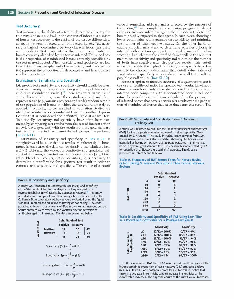
value is somewhat arbitrary and is affected by the purpose of the testing.68 For example, in a screening program to detect exposure to some infectious agent, the purpose is to detect all horses possibly exposed to that agent. In such cases, choosing a lower cutoff value will maximize test sensitivity and minimize the number of false-negative results. On the other hand, an equine clinician may want to determine whether a horse is infected with a certain agent, with minimal chances of misclas-sification. In such cases the cutoff of choice will be the one that maximizes sensitivity and specificity and minimizes the number of both false-negative and false-positive results. This cutoff value that yields the highest sensitivity and specificity is fre-quently the choice. To determine that cutoff value, values of sensitivity and specificity are calculated using all test results as possible cutoff values (Box 61-12).

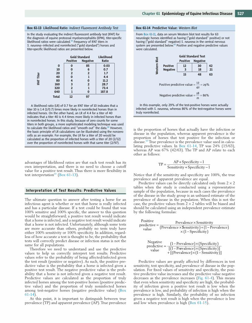
Another option to measure accuracy of a quantitative test is the use of likelihood ratios for specific test results. Likelihood ratios measure how likely a specific test result will occur in an infected horse compared with a noninfected horse. Likelihood ratios for specific test results are calculated as the proportion of infected horses that have a certain test result over the propor-tion of noninfected horses that have that same test result. The

Test Accuracy

Test accuracy is the ability of a test to determine correctly the true status of an individual. In the context of infectious diseases of horses, test accuracy is the ability of the test to differentiate correctly between infected and noninfected horses. Test accu-racy is basically determined by two characteristics: sensitivity and specificity. Test sensitivity is the proportion of infected horses correctly identified by the test as infected. Test specificity is the proportion of noninfected horses correctly identified by the test as noninfected. When sensitivity and specificity are less than 100%, their complement (1 − sensitivity and 1 − specific-ity) represent the proportion of false-negative and false-positive results, respectively.

Estimation of Sensitivity and SpecificityDiagnostic test sensitivity and specificity should ideally be char-acterized using appropriately designed, population-based studies (test validation studies).67 There are several variations in study designs, but in general, these studies should include a representative (e.g., various ages, gender, breeds) random sample of the population of horses in which the test will ultimately be applied.67 Typically, horses enrolled in validation studies are identified as infected or noninfected based on another diagnos-tic test that is considered the definitive, “gold standard” test. Traditionally, sensitivity and specificity have often been esti-mated by comparing test results from the test of interest (often a newly developed test) with the results from the gold standard test in the infected and noninfected groups, respectively (Box 61-11).

Estimation of sensitivity and specificity in Box 61-11 is straightforward because the test results are inherently dichoto-mous. In such cases the data can be simply cross-tabulated into a 2 × 2 table and the values for sensitivity and specificity cal-culated. However, when test results are quantitative (e.g., titers, white blood cell counts, optical densities), it is necessary to determine a cutoff value for a positive test result in order to estimate test sensitivity and specificity. The choice of a cutoff

Box 61-11 Sensitivity and Specificity

A study was conducted to estimate the sensitivity and specificity of the Western blot test for the diagnosis of equine protozoal myeloencephalitis (EPM) caused by Sarcocystis neurona.63 This study included serum samples from 63 neurologic horses necropsied at the California State Laboratory. All horses were evaluated using the “gold standard” method and classified as having or not having S. neurona parasites or lesions characteristic of EPM in their central nervous system. Serum samples were tested by the Western blot for detection of antibodies against S. neurona. The data are presented below.

Sensitivity (Se) %= =1215

80

Specificity (Sp) %= =1848

38

False-negative Se( ) %1 315

20− = =

False-positive Sp( ) %1 3048

62− = =

Wes

tern

Blo

t Gold Standard Test

Positive Negative

Positive 12 30 42Negative 3 18 21

15 48 63

Box 61-12 Sensitivity and Specificity: Indirect Fluorescent Antibody Test

A study was designed to evaluate the indirect fluorescent antibody test (IFAT) for the diagnosis of equine protozoal myeloencephalitis (EPM) caused by S. neurona.64 The study included serum samples from 109 horses necropsied at the California State Laboratory. All horses were identified as having or not having S. neurona parasites in their central nervous system (gold standard test). Serum samples were tested by IFAT for detection of antibody titers against S. neurona. The data are presented in Tables A and B below.

Table A. Frequency of IFAT Serum Titers for Horses Having or Not Having S. neurona Parasites in Their Central Nervous System

Table B. Sensitivity and Specificity of IFAT Using Each Titer as a Potential Cutoff Value for a Positive Test Result

In this example, an IFAT titer of 20 was the test result that yielded the lowest combined proportion of false-negative (0%) and false-positive (6%) results and is one potential choice for a cutoff value. Notice that there is a decrease in sensitivity and an increase in specificity as the cutoff value increases. The opposite occurs as the cutoff value decreases.

Cuto

ff V

alue

for

a

Posi

tive

Res

ult

Sensitivity Specificity

≥0 12/12 = 100% 0/97 = 0%≥10 12/12 = 100% 85/97 = 88%≥20 12/12 = 100% 91/97 = 94%≥40 10/12 = 83% 93/97 = 96%≥80 9/12 = 75% 93/97 = 96%≥160 6/12 = 50% 94/97 = 97%≥320 3/12 = 25% 96/97 = 99%≥640 1/12 = 8% 97/97 = 100%

IFAT

TIT

ER

Gold StandardPositive Negative

0 0 8510 0 620 2 240 0 180 4 0

160 3 2320 2 1640 1 0

Total 12 97

527Chapter 61 Epidemiology of Equine Infectious Disease

is the proportion of horses that actually have the infection or disease in the population, whereas apparent prevalence is the proportion of horses that test positive for the infection or disease.43 True prevalence is the prevalence value used in calcu-lating predictive values. In Box 61-14, TP was 24% (15/63), whereas AP was 67% (42/63). The TP and AP relate to each other as follows:

TPAP Specificity

Sensitivity Specificity=

+ −+ −

11

Notice that if the sensitivity and specificity are 100%, the true prevalence and apparent prevalence are equal.

Predictive values can be directly calculated only from 2 × 2 tables when the study is conducted using a representative sample of the population, because in such cases the prevalence of the disease in the study group is an unbiased estimate of the prevalence of disease in the population. When this is not the case, the predictive values from 2 × 2 tables will be biased and should be calculated using an independent prevalence estimate by the following formulas:

Positivepredictive

value

Prevalence SensitivityPrevalence

=×

×( SSensitivity PrevalenceSpecificity

) ( )( )

+ −× −

11

Negativepredictive

value

Prevalence SpecificityPr

=− ×−

( ) ( )[(

11 eevalence SpecificityPrevalence Sensitivity

) ( )][( ) ( )]

×+ × −1

Predictive values are greatly affected by differences in test sensitivity, test specificity, and prevalence of disease in the pop-ulation. For fixed values of sensitivity and specificity, the posi-tive predictive value increases and the predictive value negative decreases as the prevalence increases (Fig. 61-4). This means that even when sensitivity and specificity are high, the probabil-ity of infection given a positive test result is low when the prevalence is low, and probability of infection is high when the prevalence is high. Similarly, the probability of no infection given a negative test result is high when the prevalence is low and low when prevalence is high (Box 61-15).

Box 61-13 Likelihood Ratio: Indirect Fluorescent Antibody Test

In the study evaluating the indirect fluorescent antibody test (IFAT) for the diagnosis of equine protozoal myeloencephalitis (EPM), titer-specific likelihood ratios were calculated.64 Frequency of IFAT titers in S. neurona–infected and noninfected (“gold standard”) horses and titer-specific likelihood ratios are presented below.

A likelihood ratio (LR) of 0.7 for an IFAT titer of 10 indicates that a titer 10 is 1.4 (1/0.7) times more likely in noninfected horses than in infected horses. On the other hand, an LR of 4.4 for a titer of 40 indicates that a titer 40 is 4.4 times more likely in infected horses than in noninfected horses. In this study, because of zero counts for some titers in both groups, a more sophisticated modeling technique was used to calculate the likelihood ratios and “smooth out” the data.64 However, the basic principle of LR calculations can be illustrated using the nonzero cells as an example. For example, the LR for a titer of 20 would be calculated as the proportion of infected horses with a titer of 20 (2/12) over the proportion of noninfected horses with that same titer (2/97).

IFAT

Tit

er

Gold Standard LikelihoodPositive Negative Ratio

0 0 85 0.0310 0 6 0.720 2 2 1.740 0 1 4.480 4 0 11.2

160 3 2 28.7320 2 1 73.4640 1 0 187.8

Total 12 97

advantages of likelihood ratios are that each test result has its own interpretation, and there is no need to choose a cutoff value for a positive test result. Thus there is more flexibility in test interpretation64 (Box 61-13).

Interpretation of Test Results: Predictive Values

The ultimate question to answer after testing a horse for an infectious agent is whether or not that horse is really infected and has a particular disease. If a test could be found that was 100% sensitive and 100% specific, the answer to this question would be straightforward; a positive test result would indicate that a horse is infected, and a negative test result would indicate that a horse is not infected. Unfortunately, although some tests are more accurate than others, probably no tests truly have either 100% sensitivity or 100% specificity. In addition, regard-less of how accurate a test is thought to be, the probability that tests will correctly predict disease or infection status is not the same for all populations.

Therefore we need to understand and use the predictive values to help us correctly interpret test results. Predictive values refer to the probability of being affected/infected given the test result (positive or negative). As such, the positive pre-dictive value is the probability that a horse is infected given a positive test result. The negative predictive value is the prob-ability that a horse is not infected given a negative test result. Predictive values are calculated as the proportion of truly infected horses among the test-positive horses (positive predic-tive value) and the proportion of truly noninfected horses among test-negative horses (negative predictive value) (Box 61-14).

At this point, it is important to distinguish between true prevalence (TP) and apparent prevalence (AP). True prevalence

Box 61-14 Predictive Value: Western Blot

From Box 61-11, data on serum Western blot test results for 63 neurologic horses identified as having (“gold standard” positive) or not having (“gold standard” negative) S. neurona in the central nervous system are presented below.63 Positive and negative predictive values were calculated.

Positive predictive value = =1242

29%

Negative predictive value = =1821

86%

In this example, only 29% of the test-positive horses were actually infected with S. neurona, whereas 86% of the test-negative horses were truly noninfected.

Wes

tern

Blo

t Gold Standard Test

Positive Negative

Positive 12 30 42Negative 3 18 21

15 48 63

528 Section 6 Prevention and Control of Infectious Diseases

When likelihood ratios for specific test results are used instead of sensitivity and specificity, the probability of disease for each specific test result can be calculated using the following formula:

Probability of disease given a specific test result

Preva=

( llence/ P Likelihood ratioPrevalence/ Prevalence Likel

11

− ×− ×

)( iihood ratio) +1

Using Tests in Combination

Frequently, two or more tests are used in the diagnosis of disease or infection. The tests can be used simultaneously or in sequence, and the results can be interpreted in parallel or in series. In parallel interpretation, horses testing positive in one or more tests are considered positive.43 For example, horses might be considered infected with Salmonella enteritidis after testing positive in at least one of several fecal cultures performed in sequence. In series interpretation, horses are considered positive only if they test positive in all tests.43 For example, horses tested for EPM might be considered infected only if they test positive for S. neurona antibodies in serum and in cerebrospinal fluid (CSF). Note that the serum and CSF tests can be run simultane-ously or in sequence when a CSF test is run only in seropositive horses. When multiple tests are used, the sensitivity and speci-ficity of the combination of tests are different than the sensitiv-ity and specificity of each test separately. In parallel interpretation the combination of tests has higher sensitivity but lower speci-ficity than each individual test. In series interpretation the com-bination of tests has lower sensitivity and higher specificity than each individual test.

Other Diagnostic Test Characteristics

Other characteristics of diagnostic tests that should be evaluated before or concomitantly with population-based accuracy studies include analytical sensitivity and specificity and reliability. Ana-lytical sensitivity indicates the minimum detectable amount of the material (e.g., antibodies, antigens) being measured by the test. Analytical specificity indicates the potential for cross-reactivity with materials of no interest. Analytical sensitivity and specificity are assessed in laboratory conditions and affect the population estimates of sensitivity and specificity; however, they are different quantities. For example, information on the minimum amount of serum antibodies detected by an ELISA test for the diagnosis of a certain disease might be important to establish the optimum serum dilution to be used in the plaques when testing field samples. Similarly, samples from animals infected with various potential cross-reacting agents should be tested to assess occurrence of false-positive results.

Reliability is the ability of the test to produce the same results when samples are tested multiple times in the same laboratory (repeatability) or in different laboratories (reproduc-ibility).43 There are various measures of reliability, including the coefficient of variation and the correlation coefficient for quan-titative tests and the kappa measure of agreement for qualita-tive tests.43

Overall, these measures assess how concordant test results are in multiple testing.

Strategies for Prevention of Infectious Disease

In general, prevention of infectious disease involves altering the host, agent, or environment to make it more difficult for disease to occur or spread. We usually have little control over the

Figure 61-4 Relationship among positive predictive value (PVP), negative pre-dictive value (PVN), and prevalence.

100%

90%

80%

70%

60%

50%

40%

30%

20%

10%

0%0% 10% 20% 30% 40% 50%

Prevalence

60% 70% 80% 90% 100%

Pre

dict

ive

valu

e

PVPPVN

Box 61-15 Predictive Value: Enzyme-Linked Immunosorbent Assay

Assume a hypothetical scenario in which two populations of neurologic horses (i.e., from two veterinary hospitals in different parts of the country) were serologically tested for diagnosis of West Nile virus (WNV) infection. In Population 1, independent virus isolation studies have shown that the true prevalence of WNV is 1%, and in Population 2, the same studies have shown that WNV true prevalence is 90%. Both populations were tested with the same test, an enzyme-linked immunosorbent assay (ELISA), for detection of antibodies against WNV and determination of the infection status. Assume that the test has been shown to be 90% sensitive and 90% specific and that 1000 horses from each population were tested. The 2 × 2 tables below show the data for each population. The data in each cell of these 2 × 2 tables were distributed based on the prevalence and test characteristic information.

Positive predictive value = =9108

8%

Negative predictive value = =891892

99%

Positive predictive value = =810820

99%

Negative predictive value = =90180

50%

Despite the use of the same test, the probability that a test-positive horse is infected in Population 1 is only 8%, compared with the 99% in Population 2. This means that the majority (99/108) of the test-positive horses in Population 1 were actually false-positive results. Similarly, the probability that a test-negative horse is actually not infected in Population 1 is 99% versus 50% in Population 2. Therefore 50% of the test-negative horses in Population 2 were actually infected and were false-negative results.

ELIS

A

Population 1 Infected

Yes No

Positive 9 99 108Negative 1 891 892

10 990 1000

ELIS

A

Population 2 Infected

Yes No

Positive 810 10 820Negative 90 90 180

900 100 1000

529Chapter 61 Epidemiology of Equine Infectious Disease

typically seen? Compute an attack risk (attack rate), as described earlier, and compare it to the normal or expected occurrence of disease, if known.

5. Describe the outbreak temporally, spatially, and by animal characteristics. Examine the temporal characteristics of the outbreak by creating an epidemic curve (see section on Temporal Patterns of Disease). Use the client’s calendar to obtain the most accurate information on disease onset. Ask the following questions: Does it appear to be a point-source or a propagated epidemic? Does disease onset coincide with any management changes or recent additions to the farm? Describe disease spatially by making a map recording the total number of horses in each region (e.g., field, pasture, barn, farm) and the number of ill horses in each region. Be sure to record the location of feed and water sources on the map, as well as locations where horses might come in contact with wildlife or other livestock species. Record age, gender, breed, vaccination status, use, housing type, loca-tion, and feed and water sources of all animals in the population—those unaffected as well as those affected.

6. Analyze data. For each factor of interest (age, gender, breed, vaccination status, use, housing type, location, feed and water sources), construct an attack risk table, as described earlier. Look for differences among groups. Which factor has the strongest association?

7. Working hypothesis. Based on data analyses, develop hypotheses regarding the type of epidemic that is occurring (point-source versus propagated), the source of the epi-demic, and possible modes of spread (e.g., direct contact, vector, fomites).

8. Implement disease controls. Standard disease control mea-sures include mass treatment, quarantine, environmental hygiene, mass immunization, and applied ecology.69 Mass treatment, such as administration of antimicrobials during a Salmonella outbreak, is intended to reduce transmission of disease by decreasing the amount and duration of shed-ding by infectious individuals and decreasing the likelihood of infection in susceptible animals. Quarantine restricts movement of horses suspected of being infectious; it is intended to reduce the likelihood that infected horses will come in contact with susceptible horses. Environmental hygiene incorporates actions that remove or prevent envi-ronmental contamination, reducing the likelihood of disease exposure for horses in that environment; use appropriate cleaning agents, and rinse thoroughly. Mass immunization (vaccination) acts to decrease the susceptibility of both the individual horse and the herd (through herd immunity). Applied ecology refers to disease control methods that target some factor other than the disease agent, such as the vector or the disease reservoir; the goal is to reduce the likelihood that horses will be exposed to disease. To apply these methods, an understanding of the disease’s life cycle is important.

9. Intensive follow-up. Intensive follow-up includes confirma-tion of the diagnosis (clinical, pathologic, or microbiologic data) and confirmation of the disease source (microbiologic or toxicologic examination of feeds, fomites, or suspect carrier horses) if possible. Detailed diagrams or flowcharts of animal movements or feed preparation and distribution may be helpful in identifying points where preventive mea-sures could be implemented.

10. Report. Summarize findings, and present them to the client. Colleagues and local veterinary associations may also be interested in the investigation and its results.

The complete reference list is available online at www. expertconsult.com.

disease agent, so we focus on the disease host (the horse) and its environment. A herd is best able to resist infection if the horses in it are immunized, properly nourished, and minimally stressed. An environment in which new equine arrivals are quarantined, tested for disease, and immunized before mixing with the herd minimizes the likelihood of introduction of a new disease, as does an environment where contact between disease vectors (e.g., mosquitoes, ticks) and horses is minimized. Disease spread is more easily controlled in a well-ventilated environ-ment with easily cleanable, nonporous surfaces. Standing water in which mosquitoes breed should be minimized. Water and feed troughs should be cleaned regularly; a contaminated trough can quickly amplify an outbreak of salmonellosis or strangles.

To prevent the arrival or spread of a specific infectious disease, an understanding of the disease’s life cycle and risk factors is important. How do horses become infected? Through a vector, as with WNV encephalitis? By direct contact, as with equine influenza? By indirect contact, as with salmonellosis? Through aerosol spread, as with equine influenza? Minimize horses’ exposure to the source of infection. How pathogenic or virulent is the disease? Does it have a lengthy incubation period, or a carrier or persistently infected state (e.g., strangles)? Iden-tify and isolate or treat asymptomatic horses that may be sources of infection. Does the disease agent survive in the envi-ronment (e.g., Salmonella)? If so, institute biosecurity measures such as foot baths to minimize environmental contamination. What are known risk factors for the disease? Is it associated with pasture grazing, as with MRLS or strongyles? Change management as necessary to minimize known risk factors for the disease.

Managing an Outbreak of Infectious Disease

An outbreak investigation is a systematic approach to identify-ing the cause(s) and source(s) of an epidemic (see Chapter 62). The goals of an outbreak investigation are to identify the problem, identify steps that can be taken immediately to deal with the problem, and identify means by which future out-breaks can be prevented. The standard steps in an outbreak investigation are described next.

1. Make a diagnosis. After initial contact with the client, review relevant diagnoses before a farm visit. For each potential diagnosis, review the biology, epidemiology, diag-nostic method, and treatment. At the farm, listen carefully and say nothing that might influence your client’s percep-tion of events. Take samples as needed, look for patterns that may be relevant, and define natural groups (housing, use, age, gender, or breed) that should be compared. Use clinical observations and test results to make a tentative diagnosis. If the initial diagnosis is a zoonotic or reportable disease, take appropriate action.

2. Verify the diagnosis. When a tentative or final diagnosis of disease has been made, ensure that it is medically sound. Use medical records, laboratory test results, and clinical examinations to confirm that the diagnosis is consistent with the information available. If the data are not consistent with the diagnosis, seek a better diagnosis.

3. Define a “case.” To facilitate identification of cases associ-ated with the outbreak, specify the clinical signs and test results that define a case of disease. Some illness in the population may be unrelated to the outbreak. By defining an outbreak-associated “case” of disease, unrelated illnesses may be excluded from analysis.

4. Determine the magnitude of the problem. Is there an epidemic? Are more horses affected by this disease than

References1. Gordis L: Epidemiology. Philadelphia, 1996, Saunders.2. Dwyer RM, Garber LP, Traub-Dargatz JL, et al: Case-

control study of factors associated with excessive propor-tions of early fetal losses associated with mare reproductive loss syndrome in central Kentucky during 2001. J Am Vet Med Assoc 222:613–619, 2003.

3. Cohen ND, Carey VJ, Donahue JG, et al: Case-control study of late-term abortions associated with mare repro-ductive loss syndrome in central Kentucky. J Am Vet Med Assoc 222:199–209, 2003.

4. Webb BA, Barney WE, Dahlman DL, et al: Eastern tent caterpillars (Malacosoma americanum) cause mare repro-ductive loss syndrome. J Insect Physiol 50:185–193, 2004.

5. Slovis NM: Clinical observations of the pericarditis syn-drome. Session 1: Field and clinical observations on MRLS. 2002, Workshop on Mare Reproductive Loss.

6. Latimer C: Endophthalmitis: a syndrome associated with mare reproductive loss syndrome? Session 1: Field and clinical observations on MRLS. 2002, Workshop on Mare Reproductive Loss.

7. Cohen ND, Donahue JG, Carey VJ, et al: Case-control study of early-term abortions (early fetal losses) associated with mare reproductive loss syndrome in central Kentucky. J Am Vet Med Assoc 222:210–217, 2003.

8. Donahue JG, Sells S, Giles R, et al: Bacteria associated with mare reproductive loss syndrome: late fetal losses. Session 2: Laboratory correlates of MRLS. 2002, Workshop on Mare Reproductive Loss.

9. Tobin T, Harkins JD, Roberts JF, et al: The mare reproduc-tive loss syndrome and the eastern tent caterpillar. II. A toxicokinetic/clinical evaluation and a proposed pathogen-esis: septic penetrating setae. J Appl Res Vet Med 2:142–158, 2004.

10. Priddy T: Mare reproductive loss syndrome: weather data. 2001, University of Kentucky.

11. Fitzgerald TD: The tent caterpillars. Ithaca, NY, 1995, Cornell University.

12. Dwyer RM: Fitting the pieces of the puzzle: mare repro-ductive loss syndrome update. Equine Vet Educ 15:45–47, 2003.

13. Schuler LA, Khaitsa ML, Dyer NW, et al: Evaluation of an outbreak of West Nile virus infection in horses: 569 cases (2002). J Am Vet Med Assoc 225:1084–1089, 2004.

14. Rossano MG, Kaneene JB, Marteniuk JV, et al: The sero-prevalence of antibodies to Sarcocystis neurona in Michigan equids. Prev Vet Med 48:113–128, 2001.

15. Pitel PH, Lindsay DS, Caure S, et al: Reactivity against Sarcocystis neurona and Neospora by serum antibodies in healthy French horses from two farms with previous equine protozoal myeloencephalitis–like cases. Vet Parasitol 111:1–7, 2003.

16. Vardeleon D, Marsh AE, Thorne JG, et al: Prevalence of Neospora hughesi and Sarcocystis neurona antibodies in horses from various geographical locations. Vet Parasitol 95:273–282, 2001.

17. Baverud V, Gustafsson A, Franklin A, et al: Clostridium dif-ficile: prevalence in horses and environment, and antimicro-bial susceptibility. Equine Vet J 35:465–471, 2003.

18. Chanter N, Talbot NC, Newton JR, et al: Streptococcus equi with truncated M-proteins isolated from outwardly healthy horses. Microbiology (Reading) 146:1361–1369, 2000.

19. Fintl C, Dixon PM, Brazil TJ, et al: Endoscopic and bacte-riological findings in a chronic outbreak of strangles. Vet Rec 147:480–484, 2000.

20. Newton JR, Verheyen K, Talbot NC, et al: Control of stran-gles outbreaks by isolation of guttural pouch carriers

identified using PCR and culture of Streptococcus equi. Equine Vet J 32:515–526, 2000.

21. Verheyen K, Newton JR, Talbot NC, et al: Elimination of guttural pouch infection and inflammation in asymptom-atic carriers of Streptococcus equi. Equine Vet J 32:527–532, 2000.

22. Borchers K, Wolfinger U, Ludwig H: Latency-associated transcripts of equine herpesvirus type 4 in trigeminal ganglia of naturally infected horses. J Gen Virol 80:2165–2171, 1999.

23. Smith DJ, Iqbal J, Purewal A, et al: In vitro reactivation of latent equid herpesvirus-1 from CD5+/CD8+ leukocytes indirectly by IL-2 or chorionic gonadotropin. J Gen Virol 79:2997–3004, 1998.

24. Borchers K, Wolfinger U, Lawrenz B, et al: Equine herpes-virus 4 DNA in trigeminal ganglia of naturally infected horses detected by direct in situ PCR. J Gen Virol 78:1109–1114, 1997.

25. Rizvi SM, Slater JD, Wolfinger U, et al: Detection and dis-tribution of equine herpesvirus 2 DNA in the central and peripheral nervous systems of ponies. J Gen Virol 78:1115–1118, 1997.

26. Edington N, Welch HM, Griffiths L: The prevalence of latent equid herpesviruses in the tissues of 40 abattoir horses. Equine Vet J 26:140–142, 1994.

27. Slater JD, Borchers K, Thackray AM, et al: The trigeminal ganglion is a location for equine herpesvirus 1 latency and reactivation in the horse. J Gen Virol 75:2007–2016, 1994.

28. Welch HM, Bridges CG, Lyon AM, et al: Latent equid herpesviruses 1 and 4: detection and distinction using the polymerase chain reaction and co-cultivation from lym-phoid tissues. J Gen Virol 73:261–268, 1992.

29. Edington N, Bridges CG, Huckle A: Experimental reacti-vation of equid herpesvirus 1 (EHV 1) following the administration of corticosteroids. Equine Vet J 17:369–372, 1985.

30. Thrusfield M: Veterinary epidemiology, ed 2, London, 1995, Blackwell Science.

31. Rothman KJ, Greenland S: Modern epidemiology, ed 2, Philadelphia, 1998, Lippincott-Raven.

32. Fine PE: Herd immunity: history, theory, practice. Epide-miol Rev 15:265–302, 1993.

33. Sebastian M, Gantz MG, Tobin T, et al: The mare reproduc-tive loss syndrome and the eastern tent caterpillar: a toxicokinetic/statistical analysis with clinical, epidemio-logic, and mechanistic implications. Vet Ther 4:324–339, 2003.

34. Hayes CG: West Nile fever. In Monath TP, editor: The arboviruses: epidemiology and ecology, Boca Raton, FL, 1989, CRC Press, pp 59–88.

35. Hubalek Z, Halouzka J, Juricova Z: West Nile fever in Czechland. Emerg Infect Dis 5:594–595, 1999.

36. Romi R, Pontuale G, Ciufolini MG, et al: Potential vectors of West Nile virus following an equine disease outbreak in Italy. Med Vet Entomol 18:14–19, 2004.

37. Work TH, Hurlbut HS, Taylor RM: Indigenous wild birds of the Nile delta as potential West Nile virus circulating reservoirs. Am J Trop Med Hyg 4:872–888, 1955.

38. Abbassy MM, Osman M, Marzouk AS: West Nile (Flaviviri-dae: Flavivirus) in experimentally infected Argas ticks (Argasidae). Am J Trop Med Hyg 48:726–737, 1993.

39. Lawrie CH, Uzcategui NY, Gould EA, et al: Ixodid and argasid tick species and West Nile virus. Emerg Infect Dis 10:653–657, 2004.

40. US Department of Agriculture, Animal and Plant Health Inspection Service: “Hot Issues”: West Nile virus. Available at http://www.aphis.usda.gov/lpa/issues/wnv/wnv.html. Accessed March 2005.

529.e1Chapter 61 Epidemiology of Equine Infectious Disease

41. Saville WJ, Reed SM, Morley PS, et al: Analysis of risk factors for the development of equine protozoal myeloen-cephalitis in horses. J Am Vet Med Assoc 217:1174–1180, 2000.

42. Meijer WG, Prescott JF: Rhodococcus equi. Vet Res 35:383–396, 2004.

43. Dohoo I, Martin W, Stryhn H: Veterinary epidemiologic research. Charlottetown, 2003, AVC.

44. Trock SC, Meade BJ, Glaser AL, et al: West Nile virus out-break among horses in New York State, 1999 and 2000. Emerg Infect Dis 7:745–747, 2001.

45. Estrada-Franco JG, Navarro-Lopez R, Beasley DWC, et al: West Nile virus in Mexico: evidence of widespread circula-tion since July 2002. Emerg Infect Dis 9:1604–1607, 2003.

46. Dauphin G, Zientara S, Zeller H, et al: West Nile: world-wide current situation in animals and humans. Comp Immunol Microbiol Infect Dis 27:343–355, 2004.

47. Zeller HG, Schuffenecker I: West Nile virus: an overview of its spread in Europe and the Mediterranean basin in contrast to its spread in the Americas. Eur J Clin Microbiol Infect Dis 23:147–156, 2004.

48. Marlenee NL, Lorono-Pino MA, Beaty BJ, et al: Detection of antibodies to West Nile and Saint Louis encephalitis viruses in horses. Salud Publica Mexico 46:373–375, 2004.

49. Salazer PL, et al: Outcome of equids with clinical signs of West Nile virus infection and factors associated with death. J Am Vet Med Assoc 225:267–274, 2004.

50. US Department of Agriculture, Animal and Plant Health Inspection Service: Equine Program information: West Nile virus in 2004. http://www.aphis.usda.gov/vs/nahps/equine/wnv/map2004.html (accessed February 2005).

51. World Organization for Animal Health (OIE): Update on avian influenza in animals in Asia (type H5). Available at http://www.oie.int/downld/AVIAN%20INFLUENZA/A_AI-Asia.htm. Accessed February 2005.

52. McQueen JL, Davenport FM, Keeran RJ, et al: Studies of equine influenza in Michigan, 1963. II. Epizootiology. Am J Epidemiol 83:280–286, 1966.

53. Rose MA: Respiratory virus infections in man and animals: equine influenza viruses isolated at Cambridge in 1963 and 1965. Proc R Soc Med 59:51–52, 1966.

54. Scholtens RG, Steele JH, Dowdle WR, et al: U.S. epizootic of equine influenza, 1963. Public Health Rep 79:393–402, 1964.

55. Kitchen RH, Kehler WH, Henthorne JC: The 1963 equine influenza epizootic. J Am Vet Med Assoc 143:1108–1110, 1963.

56. Mare CJ: Vesicular stomatitis: ecology of the disease in the USA. In Equine infectious diseases VIII. Proceedings of the Eighth International Conference, Dubai, 1998, pp 243–245.

57. Schmidtmann ET, Tabachnick WJ, Hunt GJ, et al: 1995 epizootic of vesicular stomatitis (New Jersey serotype) in the western United States: an entomologic perspective. J Med Entomol 36:1–7, 1999.

58. McCluskey BJ, Hurd HS, Mumford EL: Review of the 1997 outbreak of vesicular stomatitis in the western United States. J Am Vet Med Assoc 215:1259–1262, 1999.

59. Oldruitenborgh-Oosterbaan MM, Schipper FC, Goehring LS, et al: Pleasure horses with neurological signs: EHV1-infection or mycotoxin intoxication? Tijdschrift Dierge-neeskunde 124:679–681, 1999.

60. Morley PS, Townsend HGG, Bogdan JR, et al: Descriptive epidemiologic study of disease associated with influenza virus infections during three epidemics in horses. J Am Vet Med Assoc 216:535–544, 2000.

61. Kim LM, Morley PS, Traub-Dargatz JL, et al: Factors associ-ated with Salmonella shedding among equine colic patients at a veterinary teaching hospital. J Am Vet Med Assoc 218:740–748, 2001.

62. Daniel WW: Biostatistics: a foundation for analysis in the health sciences, ed 7, New York, 1999, Wiley.

63. Daft BM, Barr BC, Gardner IA, et al: Sensitivity and speci-ficity of Western blot testing of cerebrospinal fluid and serum for diagnosis of equine protozoal myeloencephalitis in horses with and without neurologic abnormalities. J Am Vet Med Assoc 221:1007–1013, 2002.

64. Duarte PC, Daft BM, Conrad PA, et al: Evaluation and comparison of an indirect fluorescent antibody test for detection of antibodies to Sarcocystis neurona, using serum and cerebrospinal fluid of naturally and experimentally infected, and vaccinated horses. J Parasitol 90:379–386, 2004.

65. Ostlund EN, Crom RL, Pedersen DD, et al: Equine West Nile encephalitis, United States. Emerg Infect Dis 7:665–669, 2001.

66. Durham AE, Smith KC, Newton JR: An evaluation of diag-nostic data in comparison to the results of liver biopsies in mature horses. Equine Vet J 35:554–559, 2003.

67. Greiner M, Gardner IA: Epidemiologic issues in the valida-tion of veterinary diagnostic tests. Prev Vet Med 45:3–22, 2000.

68. Greiner M, Gardner IA: Application of diagnostic tests in veterinary epidemiologic studies. Prev Vet Med 45:43–59, 2000.

69. Schwabe C: Veterinary medicine and human health, ed 3, Baltimore, 1984, Williams & Wilkins.

70. International Society for Infectious Diseases: West Nile virus updates 2004. ProMed-mail archives, 2005.

71. US Department of Agriculture, Animal and Plant Health Inspection Service: Foreign Animal Disease Report, 1998, p 66.

72. Bridges VE, McCluskey BJ, Salman MD, et al: Review of the 1995 vesicular stomatitis outbreak in the western United States. J Am Vet Med Assoc 211:556–560, 1997.

73. Hurd HS, McCluskey BJ, Mumford EL: Management factors affecting the risk for vesicular stomatitis in livestock operations in the western United States. J Am Vet Med Assoc 215:1263–1268, 1999.

529.e2 Section 6 Prevention and Control of Infectious Diseases