Equilibrium Social Distancing

Flavio Toxvaerd

University of Cambridge

May 29, 2020

ResearchI Non-pharmaceutical interventions:I Equilibrium Social DistancingI Social Distancing with Asymptomatic Infection: Beliefs,Fatalism and Testing

I Pharmaceutical interventions:I On the Management of Population Immunity w. R. Rowthorn

Social distancing...I The Great Plague of Milan (1639)

Literature on behavior in SI, SIS and SIR modelsI Reluga (2010)I Rowthorn and Toxvaerd (2012)I Fenichel et al. (2011), Fenichel (2013)I Chen et al. (2011), Chen (2012)I Gersovitz and Hammer (2004)I Chen and Toxvaerd (2014)I Greenwood et al. (2017, 2019)I Toxvaerd (2019)I New wave of literature in both macro and micro, manypresented in this workshop

The SIR modelI The SIR model equations:

S(t) = −βI (t)S(t)

I (t) = I (t) [βS(t)− γ]

R(t) = γI (t)

S(t) = 1− I (t)− R(t), S(0) = S0 > γ/β

The SIR modelI The SIR model paths:

The economic modelI Preferences over health states:

πS ≥ πR ≥ πI

I Choose exposure εi (t) ∈ [0, 1] → inf. at rate εi (t)βI (t)I Cost of social distancing is (1− εi (t))cI People discount future at rate ρ

The economic modelI Timeline of payoffs and transitions:

I Transition times follow Poisson distributions

The individual’s decision problemI Population game formulation of Reluga and Galvani (2011)I Each individual solves this problem:

maxεi (t)∈[0,1]∫ ∞0 e

−ρt {(1− pi (t))[πS − (1− εi (t))c ] + pi (t)ρVI} dt

s.t. pi (t) = εi (t)βI (t)(1− pi (t)), pi (0) = 0

I Here pi (t) ∈ [0, 1] denotes probability of infection residence ininfectious state

I NPV of transitioning into the infected state is

VI =1

ρ+ γ

[πI + γ

πRρ

]I Get πI while infected, πR while recovered (and zero ifdeceased)

The individual’s decision problemI Aggregate infection evolves according to

I (t) = I (t) [ε(t)βS(t)− γ] = 0

I Here aggregate exposure is

ε(t) ≡∫i∈S(t)

S(t)−1εi (t)di

I If εi (t) = 1 for all i ∈ S(t), ε(t) = 1 so like in epi model

The individual’s decision problemI The best response is

εi (t) =

0 for I (t) > I ∗

ε for I (t) = I ∗

1 for I (t) < I ∗

I Critical threshold given by

I ∗ ≡ ρc

β(

πS − ρπI+γπRρ+γ − c

)I With homogeneous pop., equilibrium involves mixed strategies

Heterogeneous populationI With het. pop., individuals draw costs ci ∼ F [0, c ]I Now have type-specific thresholds

I ∗(ci ) ≡ρci

β(

πS − γπI+ρπRρ+γ − ci

)I Since I ∗(ci ) increasing in ci , higher cost individuals

I More willing to tolerate risk of infectionI Wait longer before scaling back exposure

Heterogeneous populationI At prevalence I (t), all types w. I ∗(ci ) ≤ I (t) socially distanceI So infection equation becomes

I (t) = [1− Ft (I (t))] βI (t)S(t)− γI (t)

I As I (t) increases, more aggregate social distancing, whichcurbs further increase

I In equilibrium, lower cost types socially distance first andhigher cost types free-ride

I High cost types more exposed, and over-represented amongstinfected/recovered

I Thus lower cost types more likely to benefit from herdimmunity

I There is an intertemporal quid pro quo

Heterogeneous populationI To see quid pro quo, define total exposure as

πi ≡∫ ∞

0βε∗i (t)I (t)dt

=∫ ∞

0βmax{I ∗(ci ), I (t)}dt

I Two things to observe:I As others socially distance, path I (t) depressed → totalexposure lower

I Since I ∗(ci ) increasing in ci , so is total exposure πiI So high cost individuals likelier to become infected

Equilibrium social distancingI Because equilibrium decisions depend on biological andpreference parameters, can compare effects of changes

I Comparative statics for het. pop. case are:

β γ c ρ πS πI πRI ∗ — + + +/— — + +I + — 0 0 0 0 0

I Note that results wrt β and γ opposite in two models!I More infectious disease leads to more social distancing inequilibrium

I This helps dampen the epidemicI Biological model would have predicted the opposite to be true

Asymptomatic infectionI Special features of COVID-19 is high asymptomatic ratioI Estimates vary widely, but most are about a thirdI Many people get infected and recover without knowing theywere infected

I How does this change equilibrium behavior?

Asymptomatic infectionI Model as before, but fraction α ∈ [0, 1] never show symptomsI Everyone understands aggregate dynamicsI But individual who has never had symptoms cannotdistinguish b/w being susceptible or asymptomatically infectedor recovered

Asymptomatic infectionI Aggregate measures give by

Susceptible Infected RecoveredSymp.\Classes S(t) I(t) R(t)Asymptomatic αS(t) αI (t) αR(t)Symptomatic (1− α)S(t) (1− α)I (t) (1− α)R(t)

I Measures common knowledge and determine beliefs of peopleI As individuals homogeneous, probabilities of being in eachclass same as pop. frequencies

Asymptomatic infectionI How does this change individual’s problem?I Someone who knows he/she is infected or recovered does notsocially distance

I So must determine prob. of being (symptomatically)susceptible conditional on not having shown symptoms in past

I Will outline how beliefs are formed

Asymptomatic infectionI Assume that α = 1/3I Classes evolve as follows across epidemic

Asymptomatic infectionI Evolution of asymptomatic versus symptomatic classes

I Initially, lack of symptoms most likely b/c of susceptibilityI But increasingly, more likely b/c of asymptomaticity

Asymptomatic infectionI Probability of being susceptible is

σi (t) =S(t)

S(t) + α(I (t) + R(t))

I This probability mon. decreasingI Increasingly likely that individual was “lucky”, was infectedand recovered w/o knowing it

I Recall that risk faced by individual is now

(1− α)σi (t)βI (t) [(1− α) + αε(t)]

Asymptomatic infectionI Evolution of susceptibility, risk and force of infection acrossepidemic

I Important to notice that perceived risk is non-monotone!I There is rational fatalism (Philipson and Posner, 1993)

Asymptomatic infectionI Critical threshold now becomes time-dependentI Note that as σi (t) decreases, I ∗i (t) increases over timeI This is intuitive: as time passes, people w/o symptoms attachdecreasing prob. to being susceptible

I Thus increasingly tolerant of risks from exposureI This is reflected in higher critical level I ∗(t)I There is less social distancing in equilibrium wheninfection is asymptomatic

I In equilibrium, more infection but because of less distancingI Asympt. setting nests perfect info case (α = 0) and biologicalmodel (α = 1)

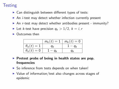
TestingI Can distinguish between different types of tests:I An i-test may detect whether infection currently presentI An r -test may detect whether antibodies present - immunity?I Let k-test have precision qk > 1/2, k = i , rI Outcomes then

mk (t) = 1 mk (t) = 0θk (t) = 1 qk 1− qkθk (t) = 0 1− qk qk

I Pretest probs of being in health states are pop.frequencies

I So inference from tests depends on when taken!I Value of information/test also changes across stages ofepidemic

TestingI Tests for immunity likely socially beneficial

I Their behavior doesn’t influence infection but costly socialdistancing reduced

I Tests for infection have ambiguous effectI Some who test positive may choose higher exposureI Thus different tests lead to different post-test beliefs andhence different post-test changes in behavior

I Difference between private and social value of tests

Back

Equilibrium social distancingI Overall view of epidemic under equilibrium social distancing:

The individual’s decision problemI The best response given by switching function

η(t)βI (t) + c = 0

I Change over time is

ddt[η(t)βI (t) + c ] = β

[η(t)I (t) + η(t)I (t)

]whereη(t) = η(t)[ρ+ εi (t)βI (t)] +

[πS − ρπI+γπR

ρ+γ − (1− εi (t))c]

I (t) = I (t) [ε(t)βS(t)− γ]ε(t) ≡

∫i∈S(t) S(t)

−1εi (t)di

I Best responses change over time as function of aggr. systemI Contrast to myopic decision making