\

Equational Programming: A Unifying Approach to Logic

and Functional Programming

Technical Report 85-030

1985

Bharat Jayaraman

The University of North Carolina at Chapel Hill Department of Computer Science New West Hall 035 A Chapel Hill. N.C. 27514

~ ~

I

Equational Programming: A Unifying Approach to Logic and Functional Programming

Abstract

Bharat Jayaraman

Department of Computer Science

UniversitJI of North Carolina at Chapel Hill

Chapel Hill, NC 1!151,4

Functional and logic languages have many similarities, but there are significant differ­

ences between them that the integration of functional and logic languages is a challenging

problem. The approach presented in this paper is called equational programming. We

show that equations can be used to define many features of functional languages, such

as abbreviations, patterns, set abstraction and infinite objects, as well as those of logic

languages, such as the ability to invert functions, unify terms, and compute with logical

variables and partially-defined values. A language called EqL is described that embod­

ies this equational approach. The formal semantics of equations is given in terms of the

complete set of solutions and the operational semantics is given in terms of two sets of

reduction rules: -t-reductions and ~-reductions. We refer to the latter form of reduction

as obiect refinement. Equations are solved by gradually refining the values bound to the

variables of the equation. This approach is amenable to parallel execution and also offers

advantages in comparison to related techniques such as narrowing.

1

I. Introduction

Logic and functional languages have emerged as two promising disciplines in pro­

gramming languages because of their high-level declarative specifications, elegant mathe­

matical properties, and potential for highly parallel execution. Despite these similarities,

each has strengths not readily possessed by the other. For example, functional languages

support infinite data structures and higher-order functions, whereas logic languages sup­

port partially-defined values and nondeterministic specifications. Thus, the integration or

"unification" of functional and logic programming has become a problem of considerable

interest recently.

Most of the existing approaches to the integration of functional and logic languages

may be considered to fall into two classes:

1. Languages that extend a logic language with functional capabilities. Within this class,

one may further distinguish two subclasses:

• Languages that are based on Hom clauses, such as Funlog [8Y84], Eqlog [GM84],

Qlog [K82], and the languages proposed by Tamaki [T84] and Barbuti et al [BBLM84].

• Languages that are based on full first-order logic, such as Tablog [MMW84] and the

language described by Hansson, et al [HHT82].

2. Languages that extend a functional language with logic capabilities. In comparison

with languages of the preceding class, these languages are generally smaller, but less

expressive. One may again distinguish two classes here:

• Languages like LOGLI8P [R882], HOPE with absolute set abstraction [D83], and

8cheme/L [80885] that support both deterministic as well as nondeterministic pro­

grams.

• Languages like FPL [BDL82], FGL+LV [L85], Qute [8883], and HA8L [H84] that

support only deterministic programs.

This paper proposes a novel approach to the problem of unifying functional and logic

languages. The difference between our proposed approach and those listed above is that we

use equations to attain the expressiveness of languages in the first class and the simplicity

of languages in the second. We consider equations because they can be used to define, in

a uniform way, common subexpressions, patterns, and infinite data structures, found in

functional languages such as FGL, HOPE, ML, and KRC [KJLR80, BM880, M84, T81],

as well as to invert functions, unify terms and compute with partially-defined values as in

2

logic languages like Prolog (WPP77]. In fact, it is possible to define any Horn clause using

equations. In addition, it is possible to directly express negation using equations. It is

worth noting that unification in logic languages is really a special form of equation solution.

Variables in such equations are logical variables, which obtain their values as a result of

solving equations. We refer to the programming paradigm arising from programming with

such equations as equational programming.

This paper also describes a novel execution strategy called object refinement. It is

well-known that the evaluator for a non-strict functional language can be based on outer­

most reduction [KLP79, H082]. However, the inclusion of logical variables and partially­

defined values requires a more general reduction strategy. Two kinds of reduction rules

for each primitive function are therefore proposed: -+-reduction is the usual reduction

rule found in non-strict functional languages, and is performed whenever argument values

are sufficiently defined for ordinary simplification. On the other hand, a "'-+-reduction is

performed when a -+-reduction cannot be applied, and refines argument values sufficiently

to enable a -+-reduction. This latter process is termed object refinement, and can be seen

as a generalization of ordinary reduction for partially-defined values, and also of conven­

tional unification for expressions that are not restricted to pure terms. An equation is

thus solved by progressively reducing its two expressions and refining objects bound to its

logical variables.

Object refinement gives many opportunities for parallel execution and also has ad­

vantages over related techniques like narrowing (H80]. Object refinement is more efficient

than narrowing because (a) reductions are performed only at the outermost level of a

term, (b) information is associated with variables and there is no need to perform sub­

stitutions on terms, and (c) only the primitive functions perform this refinement. Also,

object refinement can produce negative bindings for variables, whereas narrowing cannot.

The rest of this paper divides into the following sections: section II introduces the lan­

guage EqL and presents several examples to show the versatility of equations for functional

and logic programming; section m presents the formal semantics of the language in terms

of the complete set of solutions; section IV presents the reduction rules of the evaluator

and sketches the solution of equations; section V presents comparisons with related work;

and section VI presents conclusions and directions for further work.

3

n. Equational programming

11.1. Introducing EqL

We are developing a language called EqL which supports equational programming.

In this language we employ a functional rather than a relational or clausal syntax, primar­

ily because the components of equations are expressions which are composed of function

applications. Some potential advantages of the functional notation are that many prob­

lems for which logic languages are used are more clearly formulated using functions than

relations. Furthermore, functions possess directional information, not present in relations,

which allow them to be more executed more efficiently [R84]. Since equations allow one

to define patterns, we restrict our operation definitions to have simple variables as formal

parameters. Also, since equations may have a set of solutions we provide a set notation

similar to KRC; however, equations are used to define the "generators" and "filters". Our

language is essentially pure, lazy [HM76] first-order LISP augmented with set expressions

and equations.

The data values in this paper are limited primarily to a set of binary trees T which

are defined using two constructors leaf and cons as follows:

1. (] E T.

2. leaf{ a) E T, where a E A, a finite set of atoms.

3. x, y E T => cons(x,y) E T.

As in LISP, lists are a special form of trees and are written using the [ ... ] notation.

The element [ ] stands for the empty tree and also the empty list. We introduce the leaf

constructor for technical reasons (see section on operational semantics). However, in the

examples that follow, we will write a list of two atoms 1 and 2 as [1 2] instead of [leaf(1)

leaf(2)].

An EqL program consists of a set of operation definitions, each of which has the

following form

( opname) ( (! ormals}) <= (expression),

where (expression) is any syntactically well-formed composition of functions, which

includes the following three forms:

1. conditional-expression: if (expression) then (expression) else (expression).

2. set-expression: {(expression) I (equations)}.

4

3. where-expression: ((expression) where (equations)).

An equation has the form:

(expression) = (expression).

In this paper, a set of equations (equations) forms a conjunctive set; that is, they are

simultaneously true or false. Although disjunctive sets are useful and can be supported in

EqL, we do not consider them in this paper. Parentheses and braces both serve to delimit

the scope of logical variables appearing in equations. (There are no global variables in this

language.) We briefly explain these two constructs:

• For a where-expression ((expression) where (equations)), if expressions in the

equations are restricted to terms composed of cons, leaf, atoms and variables, then

the set of equations has a unique solution (if it exists), which is its most general unifier.

If the expressions are not just terms then any one of the set of possible solutions (if

one exists) is chosen nondeterministically. In either case the result of the where­

expression is the value of (expression) obtained after substituting for the variables in

the equations according to the (chosen) solution. (If the equations have no solution

failure is signalled, which in a sequential implementation could cause backtracking.)

• The result of a set-expression {(expression) I (equations)} is a set of values, where

each value is produced by evaluating (expression) using one of the solutions of the

set of equations. This set is represented as a list; the empty list [ ] is returned if it is '

detected that there is no solution. No order is defined among the different solutions,

and because of outermost reduction this list is produced incrementally, as needed.

11.2. Examples

We now present several examples to show the capabilities of these constructs for

functional and logic programming.

Example: Patterns

member(x, l) <= if null(l) then false else

(if eq(x,h) then true else member(x,t)

where cons(h, t) = l)

This program shows one of the simplest uses of an equation, namely, to define a

pattern which decomposes a list into its head and tail. The above definition is similar to

the LISP definition of member, except for its use of the pattern.

5

EZ4mple: Inverting functions

union(x, y) <= if null(x) then y else

(if member(h, y) then union(t, y) else cons(h, union(t, y))

where cons(h,t) = x)

{z I union([12], z) = [1 2 3]}

The above program defines the union of two sets x and y represented as lists, and

obtains the list [(1 3] (2 3] (3]) as the value of z. This is a simple example of a logic

program, illustrating how functions may be inverted.

EZ4mple: Infinite set of solutions

append(x, y) <= if null(x) then y else cons( car(x), append( cdr(x), y))

{I I append(l, [1 2]) = append((1 2], l)}

The above definition is the customary LISP definition of append, using explicit selec­

tors car and cdr. The set of solutions for the logical variable l is the infinite list [nil [1 2]

[1 2 1 2] ... ].

EZ4mple: Generators

(:prod(8t, 82) <= { cons(x, y) I member(x, s 1) = true

member(y, 82) =true}

The above function cprod defines the cartesian product of two sets 8 1 and 8 2 repre­

sented as lists. This illustrates the use of equations as "generators" to generate elements

of a set, as in KRC (T81).

EZ4mple: Set Difference

sdiff(8t,82) <={xI member(x,81) =true

member(x, 82) =false}

sdi.D{(1 2 3 6], [2 3 4 5])

The above program computes the set difference 8 1 -82 of two sets 8 1 and 8 1 represented

as lists. The above example illustrates the "generate and test" paradigm, and also shows

how negation may be stated directly. The list [1 6) is computed at the top-level.

EZ4mple: Recursive generators

perms(l) <= if null(l) then [[ ]] else

6

{cons(a,p) I member(a,l) =true

member(p,perms(sdiff(l, [a])))= true}

The above example defines the set of permutations of a list using a "recursive genera­

tor", and is again inspired by the KRC formulation of this problem [T82]. In this example

we assume that member is defined using the LISP function equal rather than eq.

Example: Generate and test

primes() <= {p I member (p, numsfrom(2)) =true

divisors(p, nums(2,p- 1)) = [ ]} numsfrom(n) <= cons(n, numsfrom(n + 1))

nums(l, h) <= if l > h then ( ] else cons(n, nums(l + 1, h))

divisors(p,l) <= {i I member(i,l) = true

mod(p, i) = 0}

The function primes above illustrates the "generate and test" paradigm for defining

the infinite set of primes. Note that the set of primes are not necessarily produced in

ascending order, and because of outermost evalution the function divisors need produce

only one divisor in order to show inequality with [ ].

Ezample: Fibonacci Sequence

addstr(8IJ 82) <= ( cons(h1 + h2, addstr(tt, t2))

where cons(hh tt) = 81

cons(h2, t2) = s2)

(fib where fib= cons(1, cons(1, addstr(fib, cdr(fib)))))

The above program expresses a solution to a problem that is easily expressed in func­

tional languages but not logic languages. The logical variable fib in the above equation

denotes an infinite list in which each successive element is generated by adding its pre­

ceding two elements of the list. Such cyclic definitions of variables are common to many

functional languages such as KRC [T81] and FGL [KJLR80], but are disallowed in most

logic languages. (Colmerauer, however, shows haw certain restricted forms of infinite trees

called rational trees may be defined in Prolog without the occur-check (C82].)

Example: Sieve of Eratosthenes

sieve(l,p) <= (if divides(h, p) then sieve(t,p) else cons(h, sieve(t,p))

7

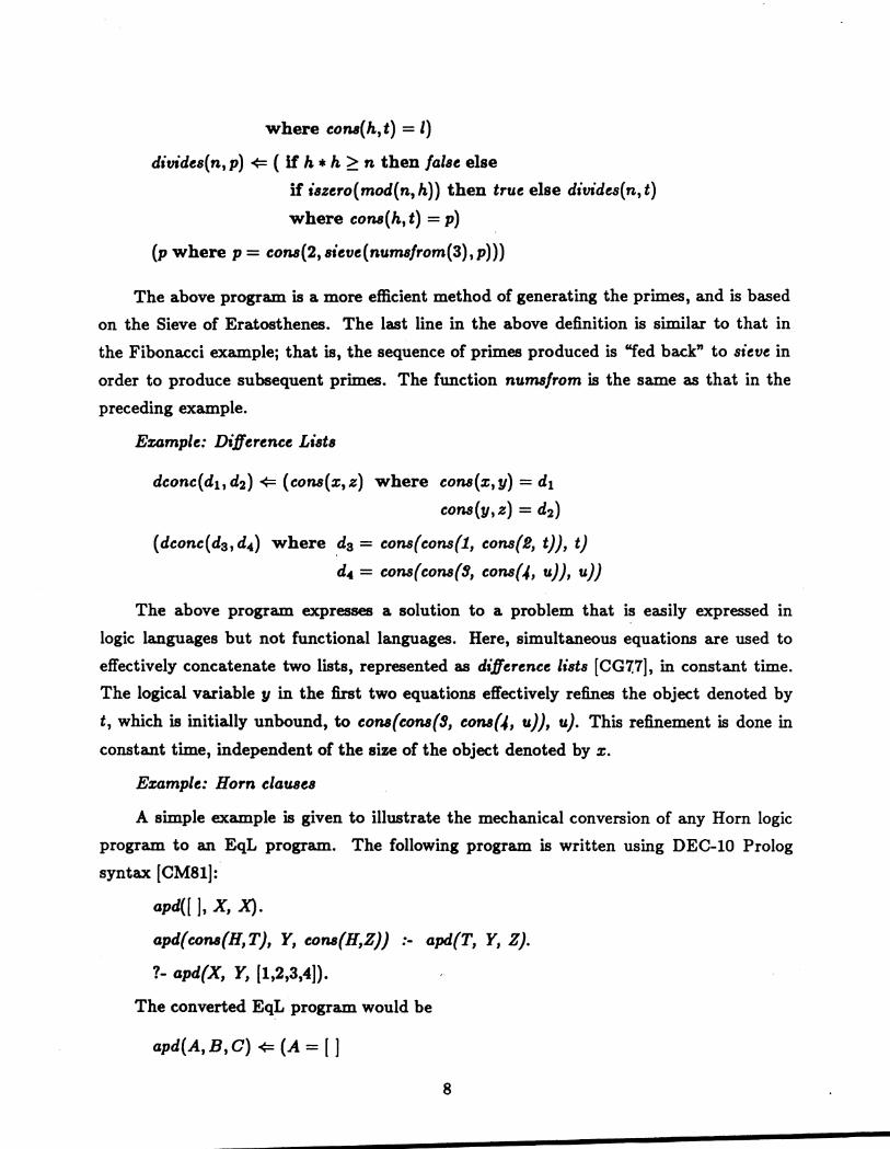
where cons(h,t) = l) divides(n,p) <= (if h * h > n then false else

if iszero(mod(n,h)) then true else divides(n,t)

where cons(h, t) = p)

(p where p = cons(2,sieve(numsfrom(3),p)))

The above program is a more efficient method of generating the primes, and is based

on the Sieve of Eratosthenes. The last line in the above definition is similar to that in

the Fibonacci example; that is, the sequence of primes produced is "fed back" to sieve in

order to produce subsequent primes. The function numsfrom is the same as that in the

preceding example.

Example: Difference Lists

dconc(dh d2) <= ( cons(x, z) where cons(x, y) = d1

cons(y, z) = d2)

(dconc(da,d4) where .ds = cons(cons{1, cons(e, t}}, t)

d4 = cons(cons{9, cons{-4, u)), u))

The above program expresses a solution to a problem that is easily expressed in

logic languages but not functional languages. Here, simultaneous equations are used to

effectively concatenate two lists, represented as difference lists (CG7;7), in constant time.

The logical variable y in the first two equations effectively refines the object denoted by

t, which is initially unbound, to cons(cons{9, cons{-4, u)}, u). This refinement is done in

constant time, independent of the size of the object denoted by x.

Example: Horn clauses

A simple example is given to illustrate the mechanical conversion of any Horn logic

program to an EqL program. The following program is written using DEC-10 Prolog

syntax (CM81):

apd(( ], X, X).

apd{cons{H,T), Y, cons(H,Z)) :- apd(T, Y, Z).

?- apd{X, Y, [1,2,3,4]).

The converted EqL program would be

apd(A, B, C) <=(A= [ ]

8

B=X

C=X)

apd(A,B,C) <= (apd(T,Y,Z) where A= cons(H,T)

B=Y

C = cons(H, Z))

{cons(X,Y) I apd{X,Y,[12 3 4]) =true}

The basic idea is to treat each predicate as a boolean-valued function. In general,

a predicate p defined by k Horn-clauses would be translated into k EqL definitions with

identical left-hand sides indicating that a nondeterministic choice is involved. Two other

points to be noted here are: (1) The expression ((equations}) returns a boolean value

indicating whether the set of equations has a solution or not. (2) The set of equations in

each definition serve to unify the goal terms with those of the clause head.

m .. Formal semantics

We now try to make precise the meaning of an EqL program. We shall restrict our

attention in this paper to the formal semantics of a set of equations. Basically, an equation

[u = v~ is true if there a substitution p such that the value denoted by ([u~p) is identical to

that for ((v~p). The semantics of an equation is then defined in terms of the complete set

of solutions, and is similar to the complete set of unifiers relative to an equational theory

[H80]. Our formalization is essentially a model-theoretic semantics'[VK76, GM84]. We

start by defining the domain G (for ground values) below:

1. 1., [ ], leal(a) E G, where a E A, the set of atoms.

2. z, y E G => cons(z, y) E G.

The partial ordering C on G is defined as follows:

1. ('v'z) .l ~ z.

2. z1 ~ z2 A Y1 C Y2 => cons(Z~tYl) C cons(z2,Y2)·

Furthermore, the limit of every infinite chain d1 C d2 ... is also in the domain. We

use 1. to denote "nontermination".

Let e be the following set of equations:

(ul = V1 . :. Un = vnD·

We first define r, the set of ground solutions of t with respect to a program P:

r = {P 1 P F= e P},

9

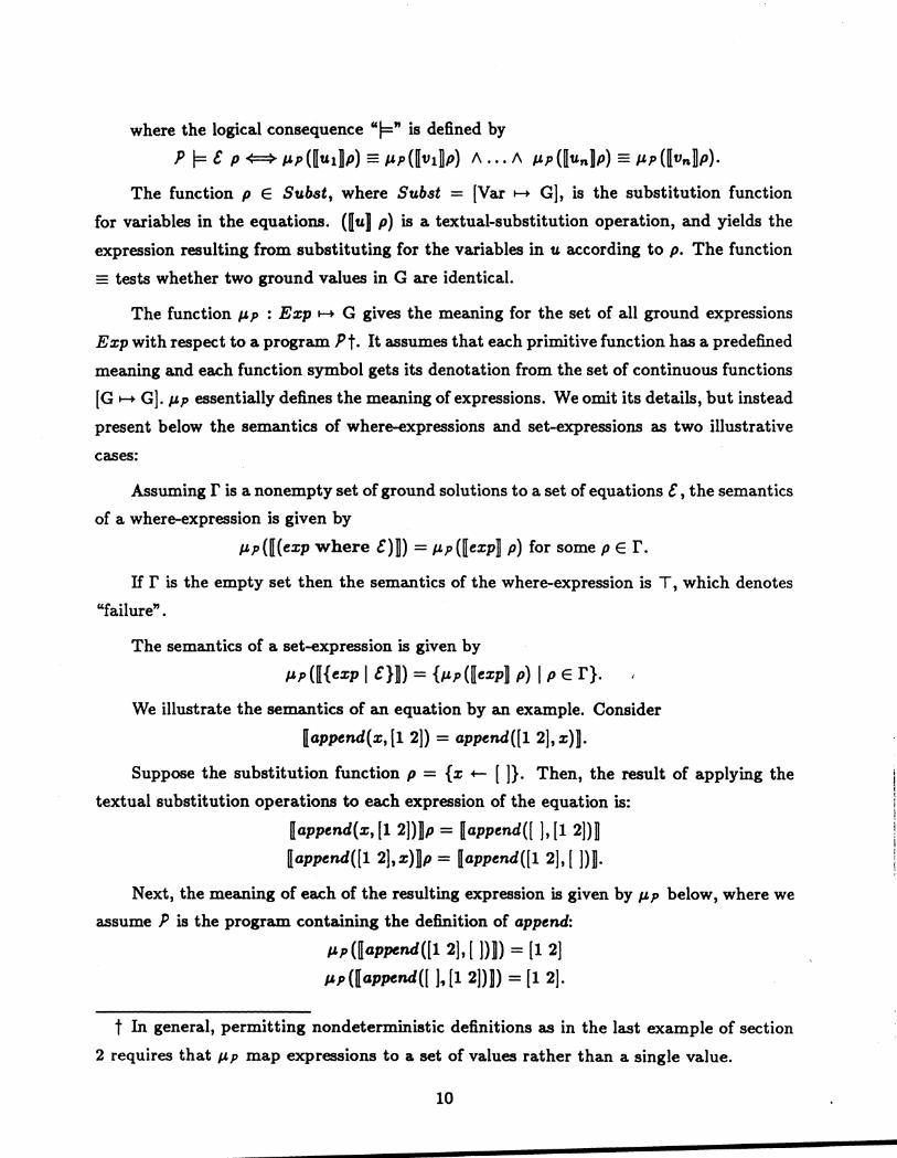
where the logical consequence "F=" is defined by

P F t P ~ #LP(ffutDP) = #Lp(ffvtDP) A.·· A #Lp(ffun]P) = #Lp(ffvnDP)·

The function p E Subst, where Subst = (Var t-+ G), is the substitution function

for variables in the equations. (ffu) p) is a textual-substitution operation, and yields the

expression resulting from substituting for the variables in u according to p. The function

= tests whether two ground values in G are identical.

The function #'P : Exp t-+ G gives the meaning for the set of all ground expressions

Exp with respect to a program Pt. It assumes that each primitive function has a predefined

meaning and each function symbol gets its denotation from the set of continuous functions

(G t-+ G]. #'P essentially defines the meaning of expressions. We omit its details, but instead

present below the semantics of where-expressions and set-expressions as two illustrative

cases:

Assuming r is a nonempty set of ground solutions to a set of equations t, the semantics

of a where-expression is given by

#'P([(exp where t)D) = #'P([exp] p) for some pEr.

If r is the empty set then the semantics of the where-expression is T, which denotes

"failure".

The semantics of a set-expression is given by

#'P([{exp I t}D) = {#'P([exp] p) I pEr}.

We illustrate the semantics of an equation by an example. Consider

[append(x, [1 2]) = append((1 2], x)J.

Suppose the substitution function p = {x +- [ ]}. Then, the result of applying the

textual substitution operations to each expression of the equation is:

[append(x, [1 2])DP = [append([ ], [1 2])D [append{[1 2],x)Dp = [append{[1 2], [])D.

Next, the meaning of each of the resulting expression is given by #LP below, where we

assume P is the program containing the definition of append:

#'P {[append{[1 2], [ ])B) = [1 2] #LP([append(( ]~[1 2]))) = [1 2].

t In general, permitting nondeterministic definitions as in the last example of section

2 requires that #'P map expressions to a set of values rather than a single value.

10

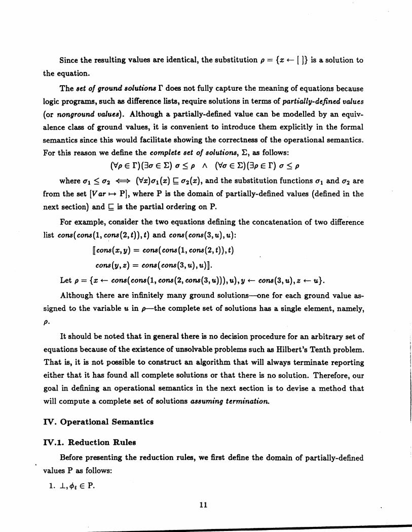
Since the resulting values are identical, the substitution p = { x +- [ ]} is a solution to

the equation.

The set of ground solutions r does not fully capture the meaning of equations because

logic programs, such as difference lists, require solutions in terms of partially-defined values

(or nonground values). Although a partially-defined value can be modelled by an equiv­

alence class of ground values, it is convenient to introduce them explicitly in the formal

semantics since this would facilitate showing the correctness of the operational semantics.

For this reason we define the complete set of solutions, E, as follows:

(V p E f) (3a E E) a < p A (Va E E) (3p E f) a ~ p

where a 1 ~ a2 <==> (Vx)al(x) ~ a2(x), and the substitution functions a 1 and a2 are

from the set (Var ~--+ P), where P is the domain of partially-defined val~es (defined in the

next section) and C is the partial ordering on P.

For example, consider the two equations defining the concatenation of two difference

list cons( cons(l, c~ns(2, t)), t) and cons( cons(3, u), u):

[ cons(x, y) = cons( cons(I, cons(2, t)), t)

cons(y,z) = cons(cons(3,u),uH.

Let p = {x +- cons(cons(I,cons(2,cons(3,u))),u),y +- cons(3,u),z +- u}.

Although there are infinitely many ground solutions--one for each ground value as­

signed to the variable u in p-the complete set of solutions has a sin,gle element, namely,

p.

It should be noted that in general there is no decision procedure for an arbitrary set of

equations because of the existence of unsolvable problems such as Hilbert's Tenth problem.

That is, it is not possible to construct an algorithm that will always terminate reporting

either that it has found all complete solutions or that there is no solution. Therefore, our

goal in defining an operational semantics in the next section is to devise a method that

will compute a complete set of solutions assuming termination.

IV. Operational Semantics

IV .1. Reduction Rules

Before presenting the reduction rules, we first define the domain of partially-defined

values P as follows:

1. j_, 4>t E P.

11

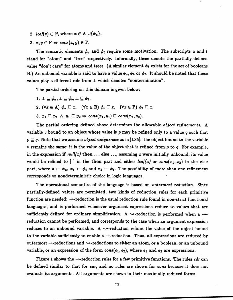
2. leal(x) E P, where x E A U{</>a}·

3. x, y E P => cons(x, y) E P.

The semantic elements <l>a and 4>t require some motivation. The subscripts a and t

stand for "atom" and "tree" respectively. Informally, these denote the partially-defined

value "don't care" for atoms and trees. (A similar element </>b exists for the set of booleans

B.) An unbound variable is said to have a value </>a, </>b or <l>t· It should be noted that these

values play a different role from .l which denotes "nontermination".

The partial ordering on this domain is given below:

1. .l !; </>a, .l C </>b, .l !; <f>t·

2. (Vx E A) </>a !; x, (Vx E B) </>b !; x, (Vx E P) </>t C x.

3. x1 !; x2 1\ Y1 C Y2 => cons(xlt Yt) !; cons(x2, Y2)·

The partial ordering defined above determines the allowable obiect refinements. A

variable v bound to an object whose value is p may be refined only to a value q such that

p!; q. Note that we assume obiect uniqueness as in (185]: the object bound to the variable

v remains the same; it is the value of the object that is refined from p to q. For example,

in the expression if null{x) then ... else ... , assuming x were initially unbound, its value

would be refined to [ ] in the then part and either leaf( a) or cons(xt, x2 ) in the else

part, where a +- </>a, x1 +- 4>t and x2 +- <l>t· The possibility of more than one refinement

corresponds to nondeterministic choice in logic languages.

The operational semantics of the language is based on outermost reduction. Since

partially-defined values are permitted, two kinds of reduction rules for each primitive

function are needed: -+-reduction is the usual reduction rule found in non-strict functional

languages, and is performed whenever argument expressions reduce to values that are

sufficiently defined for ordinary simplification. A ~-reduction is performed when a -+­

reduction cannot be performed, and corresponds to the case when an argument expression

reduces to an unbound variable. A ~-reduction refines the value of the object bound

to the variable sufficiently to enable a -+-reduction. Thus, all expressions are reduced by

outermost -+-reductions and ~-reductions to either an atom, or a boolean, or an unbound

variable, or an expression of the form cons( elt e2), where e1 and e2 are expressions.

Figure 1 shows the -+-reduction rules for a few primitive functions. The rules cdr can

be defined similar to that for car, and no rules are shown for cons because it does not

evaluate its arguments. All arguments are shown in their maximally reduced forms.

12

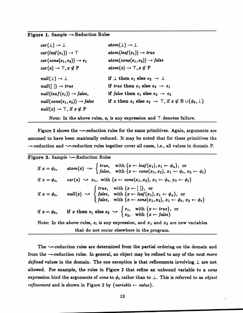
Figure 1. Sample -+-Reduction Rules

car(J.) --+ .L

car(leaf(el)) --+ T

car(cons(e1,e2))--+ e1

car(x) --+ T, x f/. P

null(.L) --+ .L

atom(.L) --+ .L

atom(leaf(el)) --+ true

atom( cons( e17 e2)) --+ false

atom(x) --+ T, x f/. P

if .L then e1 else e2 --+ .L

if true then e1 else e2 -+ e1

if false then e1 else e2 -+ e2

null ([ ]) --+ true

null(leaf(el)) --+false,

null( cons( e17 e2)) --+false

null(x) --+ T, if x f/. P

if x then e1 else e2 -+ T, if x f/. B u{ <Pb, .L}

Note: In the above rules, ei is any expression and T denotes failure.

Figure 2 shows the ~-reduction rules for the same primitives. Again, arguments are

assumed to have been maximally reduced. It may be noted that for these primitives the

-+-reduction and ~-reduction rules together cover all cases, i.e., all values in domain P.

Figure 2. Sample ~-Reduction Rules

{ true atom(x) ~ 1 1 '

1a se, with {x +- leaf(xl), x1 +- <,64 }, or with {x +- cons(xb x2), x1 +- <Pt, x2 +- <Pt}

car(x) ~ x1, with {x +- cons(x~, x2), x1 +- <Pt, x2 +- <Pt} I

{true, with {x +- [ ]}, or

null(x) ~ false, with {x +- leaf(x1), x1 +- <,64 }, or false, with {x +- cons(x1, x2), x1 +- <Pt, x2 +- <Pt}

if X= <,bt,

if X= c/>b, if th 1 { e~, with {x +-true}, or x en e1 e se e2 ~

e2, ···with {x +-false}

Note: In the above rules, ei is any expression, and x1 and x 2 are new variables

that do not occur elsewhere in the program.

The ~-reduction rules are determined from the partial ordering on the domain and

from the -+-reduction rules. In general, an object may be refined to any of the next more

defined values in the domain. The one exception is that refinements involving .L are not

allowed. For example, the rules in Figure 2 that refine an unbound variable to a cons

expression bind the arguments of cons to <Pt rather than to .L. This is referred to as object

refinement and is shown in Figure 2 by {variable +- value}.

13

IV .2. Solution of Equations

We informally present here the solution of equations by an example. Our example

shows the solution to a single equation, but since more equations are added as the solution

proceeds, the discussion is applicable to a set of equations as well. For simplicity, we omit

the leaf constructor for the atoms 1 and 2 in this example.

Consider the equation

append((1 2], x) = append(x, (1 2]). (0)

Recall that it has an infinite number of solutions: ( ], (1 2], (1 2 1 2], etc. The above

equation is just an abbreviation for

append(cons(1, cons(S, [ ])), x) = append(x, cons(1, cons(S, [ ]))). (1)

The expression on the left of equation (1) -+-reduces to

cons( car(ll), append( cdr( II), x))

where h +- cons(!, cons(2, ( ])).

The expression on the right has three possible ~-reductions, corresponding to the

three possible refinements for null(x) where x +- <Pt:

Refinement Reduced Expression

1. x +- [ ] cons(l, cons(2, [ ]))

2. z +- leaf(xl),xl +- <Pa cons(car(x),append(cdr(x),l2 ))

where 12 = cons(1, cons(2, [ ]))

3. x +- cons(xb x 2 ) cons( car(x), append( cdr(x),l2 ))

x1 +- <Pt where 12 = cons(1, cons(2, ( ]))

X2 +- </Jt

All three refinements would be considered in an actual implementation-the first in fact

leads to an overall solution-but we present here the most interesting case, which is the

equation resulting from refinement 3:

cons(car(l1),append(cdr(h),x)) = cons(car(x),append(cdr(x),l2 )) (2)

where lit l2 +- cons(1, cons(2, [ ]) ), x +- cons(xlt x2), x1 +- <Ptt and x2 +- <Pt·

This leads us to our first equation-solution rule: Whenever an equation Is of the

form cons(e1,e2) = cons(e3,e4). two new equations are oenerated: e1 = e3, and e2 = e4. (A

14

similar rule involving the constructor leaf may be defined.) The two new equations for our

example are

car(11) = car(:r:)

append( cdr( h), x) = append( cdr(:r:), h).

(3)

(4)

Equation (3) further reduces to 1 = x~, at which time x1 gets bound to 1. This

reflects a second equation-solution rule: Whenever an equation Is of the form v = e or

e = v, where v Is an unbound variable and e Is either an atom or boolean or I] or leaf(ei) or

cons(e~, e2), v Is bound to e.

Equation (4) is solved similar to equation (1). The next solution obtained is

{ x ..- cons(xh x2), XI ..- 1, x2 ..- cons(xa, x4), xa ..__ 2, X4 ..__ [ ) }

The other solutions are obtained if x 4 were refined to cons(xs, xa) and the resulting equa­

tions solved.

There is a third equation-solution rule which is applicable when both expressions

reduce to unbound variables: Whenever an equation Is of the form vi = v2 and both VI and

v 2 are unbound variables, both VI and VI are bound to the same object, whose value Is tPt·

An interesting property of the equation-solution rules is that they effectively perform

unification when the expressions are restricted to just terms. Another is that rule 1 gives

opportunities for parallel execution. However, access to common variables across equations ' that are solved in parallel must be synchronized so as not to lose any refinements. We refer

to the parallelism arising from recursively decomposing an equation into sub-equations as

cons-parallelism, which is a special form of and-parallelism. The different refinements of a

variable can be examined in parallel and gives rise to or-parallelism.

V. Related Work

The term equational programming was first introduced by Hoffman and 0 'Donnell

[H082, 085], who used it to refer to a style of function definitions by equations and a

simple semantics based on the logical consequences of equality. Unlike the logical variables

of EqL equations, the variables here are universally quantified and the equations here

are similar to abstract data type specifications. Restrictions on the left-hand sides of

equations are placed in order to insure determinacy. The term equational programming

has been recently used by Dershowitz and Plaisted to refer to a style of programming with

conditional rewrite rules [DP85] which provides the capability of first-order functional and

15

logic programming in a uniform and elegant way. Conditional expressions and equations

in EqL give all the expressive power of conditional rewrite rules, and some additional

capabilities: because variables in EqL equations may be defined cyclically, certain efficient

definitions of infinite data structures are possible, as illustrated in the Fibonacci example.

Object refinement combines the advantages of several recently proposed approaches for

executing logic languages. We summarize below the important similarities and differences:

Our reduction of expressions is similar to the pattern-driven lazy reduction of Funlog

[SY84) and the reduction strategy of FGL+LV [L85), except that no explicit unification is

performed in our approach. It is also related to Berkling's £-reduction [B85) for reducing

sets of equations that are composed of pure terms. The programs considered by Berkling

are essentially the same as EqL programs that are mechanically derived from Horn-clauses

(see example of section ll.2).

Object refinement is also related to the evaluation mechanism of Prolog with equal­

ity, proposed by Kornfeld [K83). In this language, the programmer may specify so-called

0-terms and equality theorems which get invoked whenever two terms don't unify syn­

tactically. These equality theorems in effect specify explicitly how refinements are to be

made. In EqL, these refinements are made automatically and are determined solely by the

primitive functions.

Perhaps the most closely related approach is that of narrowing [H80). It differs in two

ways form narrowing: (a) no explicit unification is performed, and '(b) reductions occur

only at the outermost level of a term. Note that narrowing is not applicable to a language

like EqL which has only simple variables as formal parameters. Also narrowing cannot

handle negative information. Recently, two variations of narrowing have been proposed:

conditional narrowing (DP85) and lazy narrowing [R85). Object refinement combines the

generality of conditional narrowing (being applicable to conditional expressions) with the

efficiency of lazy narrowing (being based on outermost reduction). The simplication steps

of conditional narrowing are analogous to our --+-reductions, and the narrowing steps are

analogous to our ~-reductions.

VI. Conclusions and Further Work

EqL supports functional programming more directly than logic programming because

of its functional syntax. However, our examples show that many logic programming

paradigms are easily stated in the language; in fact any Horn logic program can be di-

16

rectly converted to an EqL program. EqL operations have only simple variables as formal

parameters, i.e., there are no patterns, because patterns can be realized quite easily by

equations, as shown in the examples above. We provide set expressions because equations

may possess a set of solutions. In this respect, our approach is similar to that of LOG LISP

and HOPE with absolute set abstraction. The 'findall' predicate of Prolog [CM81] and

the various forms of 'all solutions' surveyed by Naish [N85] are also related. In compari­

son with these and the earlier cited works, the main contribution of our language lies in

demonstrating the clarity and power of equations for functional and logic programming.

We are at present investigating the parallel implementation of EqL. An interesting

aspect here is the implementation of set-expressions. In this implementation, we repre­

sent the tree of alternatives arising from nondeterministic choices explicitly as a tree of

frames, where each frame contains a partially-solved set of equations and corresponding

variable bindings. In this approach, and-parallelism arises within a single frame whereas

or-parallelism arises across different frames. Whenever a refinement is performed and there

is more than one choice, a frame "splits" into several frames, one for each choice. The

frames for equations that yield a solution are incorporated into the list of solutions; those

that do not are deleted. Furthermore, the list of solutions is produced incrementally, as

needed.

Also under development is a formal correctness proof of the operational semantics.

There is a strong similarity between this proof and that of theorem.2 of Hullot [H80] for

the complete set of unifiers. Essentially, the argument is as follows: If p is a solution to a

set of equations e and if all sequences of -+-reductions emanating from e p terminate, then

one can "project" each step of a sequence of ~-reductions from E on to a corresponding

step of a sequence of -+-reductions from ! p. The proof is inductive and depends on the

correctness of the ~-reductions for each of the primitive functions.

References

[A84] H. Abramson, "A Prological Definition of HASL, a Purely Functional Lan­

guage with Unification Based on Conditional Binding Expressions." In New

Generation Computing 2, 1984, pp. 3-35.

[B85] K. Berkling, "Epsilon-Reduction: Another View of Unification," In Proc. of

IFIP TC-10 Working Conference on Fifth Generation Computer Architecture,

UMIST, Manchester, July, 1985.

17

[BBLM84) R. Barbuti, M. Bellia, G. Levi, and M. Martelli, "On the Integration of Logic

Programming and Functional Programming." In Internatl. Symp. Logic Pro­

gramming, IEEE, Atlantic City, 1984, pp. 160-166.

[BDL82]

[BMS80)

[C78)

[C82)

[CG77)

[CM8lj

[D83)

[DP85)

[GM84)

M. Bellia, P. Degano, and G. Levi, "The Call by Name Semantics of a Clause

Language with Functions." In Logic Programming, Ed. K. L. Clark and S.-

A. Tirnlund, Academic Press, 1982, pp. 281-295.

R. M. Burstall, D. B. MacQueen, D. T. Sanella, "HOPE: an experimental

applicative language." In 1980 ACM LISP Conference, pp. 136-143.

K. L. Clark, "Negation as Failure." In Logic and Data Bases, Ed. H. Gallaire

and J. Minker, Plenum Press, New York, 1978, pp. 293-322.

A. Colmerauer, "Prolog and infinite trees," In Logic Programming, Ed.

K. L. Clark and S.-A. Tarnlund, Academic Press, 1982, pp. 231-251.

K. L. Clark and S. Gregory, "A First-order Theory of Data and Programs."

In Information Processing, 1977, pp. 939-944.

W. F. Clocksin and C. S. Mellish, Programming in Prolog. Springer-Verlag,

New York, 1981.

J. Darlington, "Unifying Functional and Logic Languages." Internal Report,

Imperial College, London, 1983.

N. Dershowitz and D. A. Plaisted, "Applicative Programming cum Logic

Programming." In 1985 Symp. on Logic Programming, Boston, pp. 54-66.

J. A. Goguen and J. Meseguer, "Equality, Types, Modules, and (Why Not?)

Generics for Logic Programming." J. Logic Prog. 2 (1984) pp. 179-210.

[H80) J-M. Hullot, "Canonical Forms and Unification." In Proc. 5th Workshop on

[HHT82)

[HM76]

[H082]

Automated Deduction, Springer Lecture Notes, 1980, pp. 318-334.

A. Hansson, S. Haridi, and S.-A. Tarnlund, "Properties of a Logic Program­

ming Language." In Logic Programming, Ed. K. L. Clark and S.-A. Tirnlund,

Academic Press, 1982, pp. 267-280.

P. Henderson and J. H. Morris, "A Lazy Evaluator." In Third ACM POPL,

1976, pp. 95-103.

C. M. Hoffman and M. J. O'Donnell, "Programming with Equations." ACM

TOPLAS 4, No. 1 (January 1982) pp. 83-112.

18

IJKK83]

[K82]

J.-P. Jouannaud, C. Kirchner, H. Kirchner, "Incremental Construction of

Unification Algorithms in Equational Theories." In ICALP, Barcelona, 1983,

pp. 361-373.

H. J. Komorowski, "QLOG-The Programming Environment for PROLOG in

LISP." In Logic Programming, Ed. K. L. Clark and S.-A. Tamlund, Academic

Press, 1982, pp. 315-322.

[K83] W. A. Kornfeld, "Equality for Prolog." In 8th IJCAI, Karlsruhe, West Ger­

many, 1983, pp. 514-519.

[K84] T. Khabaza, "Negation as Failure and Parallelism." In Internatl. Symp. Logic

Programming, IEEE, Atlantic City 1984, pp. 70-75.

[KJLR80] R. M. Keller, B. Jayaraman, G. Lindstrom, D. Rose, "FGL Programmer's

Guide," AMPS Technical Memo No. 1, University of Utah, July, 1980.

[L85] G. Lindstrom, "Functional Programming and the Logical Variable." In 1eth

ACM POPL, New Orleans, Jan 1985, pp. 266-280.

[MMW84] Y. Malachi, Z. Manna, and R. Waldinger, "TABLOG: The Deductive-Tableau

Programming Language," In A CM Symp. on LISP and Functional Program­

ming, Austin, 1984, pp. 323-330.

[N85] L. Naish, "All Solutions Predicates in Prolog," In Symp. on Logic Program­

ming, Boston, 1985, pp. 73-77.

[085] M. J. O'Donnell, "Equational logic as a programming language," M.I.T. Press,

1985.

[R65] J. A. Robinson, "A machine-oriented logic based on the resolution principle,"

JACM 12, pp. 23-41, 1965.

[R84] U.S. Reddy, "On the Relationship between Logic and Functional Languages,"

Draft of article to appear in Functional and Logic Programming, eds. D. De­

Groot and G. Lindstrom, 1984.

[R85]

[RS82]

U. S. Reddy, "Narrowing as the Operational Semantics of Functional Lan­

guages." In 1985 Symp. on Logic Programming, Boston, 1985, pp. 138-151.

J. A. Robinson and E. E. Sibert, "LOGLISP: Motivation, Design, and Im­

plementation." In Logic Programming, Ed. K. L. Clark and S.-A. Tarnlund,

Academic Press, 1982, pp. 299-313.

19

[SOS85]

[SS83]

[SY84]

A. Srivastava, D. Oxley, A. Srivastava, "An(other) Integration of Functional

Programming." In Proc. 1985 Symposium on Logic Programming, Boston,

1985, pp. 254-260.

M. Sa to and T. Sakurai, "Qute: A Prolog/Lisp Type Language for Logic

Programming." In 8th IJCAI, Karlsruhe, West Germany, 1983, pp. 507-513.

P. A. Subrahmanyam and J-H. You, "Conceptual Basis and Evaluation

Strategies for Integrating Functional and Logical Programming." In Inter­

nat/. Symp. Logic Programming, IEEE, Atlantic City, 1984, pp. 144-153.

[T81] D. A. Turner, "The semantic elegance of applicative languages," In ACM

Symp. on Func. Prog. and Comp. Arch., New Hampshire, October, 1981,

[T84]

[VK76]

[WPP77]

pp. 85-92.

H. Tamaki, "Semantics of a Logic Programming Language with a Reducibil­

ity Predicate." In Internatl. Symp. Logic Prog., IEEE, Atlantic City, 1984,

pp. 259-264.

M. H. van Emden and R. A. Kowalski, "The Semantics of Predicate Logic as

a Programming Language." J. ACM 23, No. 4 (1976) pp. 733-743.

D. H. D. Warren, F. Pereira, and L. M. Pereira, "Prolog: the Language and Its

Implementation Compared with LISP." SIGPLAN Notices 12, No. 8 (1977)

pp. 109-115.

20

_I