Et

Fa

b

a

ARRAA

KATEA

1

Ticpethaactatnm

dp

h0

Fluid Phase Equilibria 370 (2014) 43–49

Contents lists available at ScienceDirect

Fluid Phase Equilibria

jou rn al h om epage: www.elsev ier .com/ locate / f lu id

quation of state and artificial neural network to predict thehermodynamic properties of pure and mixture of liquid alkali metals

akhri Yousefia,∗, Hajir Karimib, Zahra Gandomkara

Department of Chemistry, Yasouj University, Yasouj 75914-353, IranDepartment of Chemical Engineering, Yasouj University, Yasouj 75914-353, Iran

r t i c l e i n f o

rticle history:eceived 11 November 2013eceived in revised form 9 February 2014ccepted 11 February 2014vailable online 22 February 2014

eywords:

a b s t r a c t

A statistical mechanical equation of state is developed to predict the volumetric properties of pure andmixture liquid alkali metals at different temperatures, pressures and compositions. The temperaturedependent parameters of the equation of state have been calculated using corresponding states correla-tion based on the normal boiling point parameters as scaling constants. It is shown that the knowledge ofjust normal boiling point and its liquid density are sufficient to estimate the thermodynamic properties ofpure and mixture liquid alkali metals in different conditions. Besides, the performance of artificial neural

lkali metalshermodynamic propertiesquation of statertificial neural network

network (ANN) based on back propagation training with 10 neurons in hidden layer for prediction ofbehavior of presented systems was investigated. A collection of 512 data points for above systems in dif-ferent temperatures and pressures was used. The Tao–Mason equation of state (TM EOS) and ANN modelresults have good agreement with the experimental data with absolute average deviations of 0.74% and0.299%, respectively.

© 2014 Elsevier B.V. All rights reserved.

. Introduction

Metals, both in liquid and vapor states, have complex structures.hey widely used in modern science and technology, includingn nuclear energetic, emission electronics, new power-intensivehemical current sources, medicine and act as coolant in nuclearower plants [1,2]. They could be also more effectively used inxtraction metallurgy, especially in that some precious metals fromheir ores and wastes [2]. These applications need the knowledge ofigh temperature properties of alkali metals because these metalsre heated to high-temperatures in these applications [3]. Thechievement of high temperature in real case is a difficult proto-ol and studying the theoretical treatment of metals is good choiceo predict and correlate the high-temperature properties of liquidlkali metals. In these circumstances the development and applica-ion of novel modeling such as equation of state and artificial neuraletwork to predict the thermodynamic properties of liquid alkalietals is great interest.

Liquid alkali metal and their alloys have been studied widely

uring the last decades by several researchers [4–11]. For exam-le Eslami [7,8] applied the Ihm–Song–Mason (ISM) equation of

∗ Corresponding author. Tel.: +98 741 222 1711; fax: +98 741 222 1711.E-mail addresses: fyousefi@mail.yu.ac.ir, mojyou54@yahoo.com (F. Yousefi).

ttp://dx.doi.org/10.1016/j.fluid.2014.02.011378-3812/© 2014 Elsevier B.V. All rights reserved.

state for pure alkali metals and their alloys using the correspond-ing states correlation based on heat of vaporization and the freezingpoint density. A perturbed hard sphere EOS has been developedfor pure alkali metals by Maftoon-Azad et al. [9]. Six hundred andninety four data points at different pressures and temperatures areexamined and the average absolute deviation of predicted liquiddensity data compared to experiments is 1.41%. Besides, Mozaffariet al. [11] extended this equation of state to calculate the liquiddensity of alkali metal alloys over a wide range of temperature.Mousazadeh et al. [12] focused on application of perturbed-chainstatistical associating fluid theory (PC-SAFT) for prediction of pureand mixtures alkali metal properties. It was found that the methodefficiently is able to predict the density of binary and ternary alkalimetal alloys of Cs–K, Na–K, Na–K–Cs, at various temperatures inthe range of freezing point up to several hundred degrees above theboiling point. Besides, Moosavi and Sabzevari [13] extended a newequation of state (EOS) which reported for pure liquid alkali metals[14] to predict the density and other thermodynamic properties ofbinary molten alloys of Na–K and Cs–K in range of freezing point upto several hundred degrees above the boiling point using quadraticmixing rules along with the mean geometry approximation (MGA).

However different authors used different equations of state(EOS) and auxiliary methods to predict and reproduce the ther-modynamic properties of these systems. Some of these attemptsare restricted to the limited ranges of temperature and pressure

4 se Equ

as

ipatntacar

dAfie

[[ctsarbo

tate

2

2

vvsEpais

w

A

A

�

wtup

Bie

4 F. Yousefi et al. / Fluid Pha

nd their results to predict the thermodynamic properties of theseystems show different degrees of accuracy.

However, in spite of their applicability there are some lim-tations with these models due to using of many adjustablearameters or mixing rules that they sometimes need a sufficientmount of data for calibration and validation purposes that makeshem computationally inefficient. In such cases, an artificial neuraletwork (ANN) can be a suitable alternative to model the differenthermodynamic properties. The relationship between the physicalnd thermodynamic properties is highly nonlinear, and an artifi-ial neural network (ANN) is an especially efficient algorithm topproximate a certain function (such as density) by learning theelationships between the input and output vectors [15].

Accordingly, ANN method can be an alternative tool to model theifferent thermodynamic properties [16,17]. In the past decades,NNs have been intensively used in various fields. The major reason

or this rapid growth and diverse applications of neural networkss their ability to virtually approximate any function in a stable andfficient way.

In the previous studies, Tao–Mason equation of state TM EOS18] has been successfully extended to fluid and fluid mixtures19–22]. Besides, the applications of equation of state and artifi-ial neural networks approaches [15,23] were studied to estimatehe properties of pure polymers. Generally, ANN is powerful anduccessful method for complex non-linear systems due to uniquedvantages such as high speed, simplicity and large capacity whicheduce engineering attempt. In recent years, ANN modeling haseen successfully used for prediction of thermophysical propertiesf pure and mixture fluids [24–27].

This research focus on the capability of both TM EOS and ANNo estimate of thermodynamic properties of liquid alkali metalsnd their alloys in different temperatures, pressures and mole frac-ions. Finally, the efficiency of these approaches is compared withxperimental data and other equations of state.

. Theory

.1. Tao–Mason equation of state

In most cases, the common equations of state are based on thean der Waals family of cubic equations, the extended family ofirial equations, or equations based more closely on the results fromtatistical mechanics and computer simulations [28–30]. The TMOS falls in the latter category. In 1994, Tao and Mason described aerturbation correction term which affect on the attractive forcesnd combined it with the ISM equation of state [31] to present anmproved equation of state (TM EOS) [18]. The TM EOS for pureubstances is as follow:

P

�KT= 1 + (B2 − ˛)� + ˛�

1 − �b�+ A1( ̨ − B)b�2 (e�TC /T − A2)

1 + 1.8(b�)4(1)

here

1 = 0.143

2 = 1.64 + 2.65[e(�−1.093) − 1]) (2)

= 1.093 + 0.26[(ω + 0.002)1/2 + 4.50(ω + 0.002)] (3)

here, ω is the Pitzer acentric factor, � is an adjustable parame-er, � is the number density, Tc is the critical temperature, kT hassual meaning, B2 is the second virial coefficient, ̨ is the scalingarameter, and b is the effective van der Waals co-volume.

The TM EOS requires the usage of the second virial coefficient,2, along with the parameters ˛, and b. It should be mentioned that

f the intermolecular potential is not available, the knowledge ofxperimental second virial coefficient data is sufficient to calculate

ilibria 370 (2014) 43–49

values of the other two temperature-dependent parameters [18].In this case, there are several correlation scheme, usually based onthe corresponding state principal that lead to the calculation of thesecond virial coefficient.

Tao and Mason formulated ˛, and b in terms of the Boyle tem-perature (TB) and the Boyle volume (vB).

˛

VB= a1e−c1

(T

TB

)+ a2

[1 − e

−c2/(

TTB

)1/4](4)

b

VB= a1

[1 − c1

(T

TB

)]e−c1

(T

TB

)

+ a2

⎧⎨⎩1 −

[1 + c2

4(

TTB

)1/4

]e

−c2(T

TB

)1/4

⎫⎬⎭ (5)

where the constant a1, a2, c1, c2 are −0.0648, 1.8067, 2.6038, 0.9726,respectively.

In the absence of sufficient experimental data, the B2 values canbe calculated from the Tsonopolous correlation [32].

B2

(PC

RTC

)= f (0)(Tr) + ωf (1)(Tr) (6)

f (0)(Tr) = 0.1445 − 0.330Tr

− 0.1385

T2r

− 0.0121

T3r

(7)

f (1)(Tr) = 0.0637 + 0.331

T2r

− 0.423

T3r

− 0.008

T8r

(8)

To achieve the higher accuracy, a corresponding state correla-tion was investigated in order to TM EOS could be applied to alkalimetals and their alloys. In this respect, the following correlationequation for B2 using new scaling parameters (such as tempera-ture and molar density at the boiling point) has been developed.The resulting correlation for second virial coefficient is presentedas follow:

B2�bp = 1.033 − 3.0069

(Tbp

T

)− 10.588

(Tbp

T

)2

+ 13.096

(Tbp

T

)3

− 9.8968

(Tbp

T

)4

(9)

where �bp and Tbp are density and temperature at boiling point.Tao and Mason observation show that the dimensionless quan-

tities ˛/�B and b/�B as almost universal functions of the reducedtemperature (T/TB) can be calculated from the exponential formu-las based on a LJ(12-6) model potential [18]. At this point the scalefactors (TB and �B) are the Boyle temperature and Boyle volume,which can be expressed in terms of the boiling point parameters.The empirical equations given in Ref. [18] for ˛/�B and b/�B as afunction of T/TB can be rescaled by Tbp and �bp, temperature anddensity in boiling point, instead of TB and �B as Eslami [33].

˛�bp = a1e−c1

(T

Tbp

)+ a2

⎡⎣1 − e

−c2/

(T

Tbp

)1/4⎤⎦ (10)

b�bp = a1

[1 − c1

(T

Tbp

)]e−c1

(T

Tbp

)

+a2

⎧⎪⎪⎨1 −

⎡⎢⎣1 + c2( )1/4

⎤⎥⎦ e

−c2(T

Tbp

)1/4

⎫⎪⎪⎬(11)

⎪⎪⎩ 4 T

Tbp

⎪⎪⎭where the constants a1, a2, c1, c2 are −0.0860, 2.3988, 0.5624,1.4267, respectively. Therefore, known value of the boiling point

se Equ

pp

m

c

G

w

aKrttu˚cnap

˚

�

T

w

oepm

(

(

d

2

n

dvlpwbatb

F. Yousefi et al. / Fluid Pha

arameters make permit to determine the temperature-dependentarameters of the equation of state.

In the previous study, TM EOS was extended to the refrigerantixtures with following equation [19].

P

�KT= 1 + �

∑ij

xixj((B2)ij − ˛ij) + �∑

ij

xixj˛ijGij + �∑

ij

xixj(I1)ij

(12)

The Gij term (the pair distribution function) in last equation wasalculated by Ihm et al. as follow: [31]:

ij = 11 − �

+[

bibj

bij

]1/3�∑

K xK b2/3K (�K − (1/4))

(1 − �)(1 − �∑

K xK bK �K )(13)

here � is the packing fraction of the mixture:For a pure system, I1 = ( ̨ − B2)�(T)˚(b�) which ˚(b�) and �(T)

re temperature dependence and density dependence parameters.nowledge of (I1)ij is required for the calculation of phase equilib-ia. Its behavior is less clear than Gij because they have inferredhe expression for �(T) and ˚(b�) from model calculations ratherhan from basic principles. A simple but reasonable procedure is tose a one fluid approximation for �(T), and an approximation for(b�) that maintains the correct explicit dependence of the virial

oefficients on mole fractions. Because the magnitude of �(T) doesot vary over a wide range, Tao and Mason [18] expect that almostny reasonable approximation for �mix will prove adequate. Thesearameters could be presented as follow [18]:

mix = �∑

K xK bK

1 + 1.8�4(∑

K xK bK

)4(15)

mix = 0.143[

exp(

�mixTcmix

T− A2mix

)](16)

That

cmix =∑

KxK TcK (17)

here Tcmix is the traditional pseudocritical temperature.In the present method, the second virial coefficient and the

ther two temperature-dependent parameters evaluation can bextended to mixtures using simple arithmetic mean of meltingoint temperature and geometric mean of liquid density at theelting point; i.e.,

Tbp)ij

= ((Tbp)i(Tbp)

j)1/2 (18)

�bp)−1/3ij

= 12

[(�bp)−1/3i

+ (�bp)−1/3j

] (19)

The adjustable parameter (�) obtains from PVT data at highensity and permits the whole procedure self-correcting.

.2. ANN modeling

Several applications and good descriptions of artificial neuraletwork (ANN) were presented in prior publications [34,35].

In ANN, the first layer constitutes the input layer (indepen-ent variables) and last one forms the output layer (dependentariables). One or more neuron layers called hidden layers can beocated between them. In this work, input variables are the tem-erature (T) pressure (P), composition (xi) and average moleculareight (MWavg) of each mixture. The structure of an ANN is defined

y number of its layers, number of neurons (nodes) in each layernd the nature of learning algorithms and neurons transfer func-ions. The key step in development of an ANN model, achieve theest condition for ANN structure. In this research, the number of

ilibria 370 (2014) 43–49 45

neurons in the hidden layers and calibration method were chosenas design variables in the network development.

2.3. Network training and selection of best network architecture

The most common neural network approach in solving prob-lems is multilayer perceptrons (MLP). The MLP learns the datapattern using an algorithms known as “training”, these algorithmsmodify weights of the neurons according to the error between thevalues of actual output and target output where provide non-linearregression between inputs and outputs variables and are extremelyuseful in recognizing patterns in complex data. An example of train-ing algorithms is the back-propagation algorithm that widely usedto train of ANN in various applications.

“Tansig” and “Purelin” were used as transfer functions in the hid-den layer; and output layer respectively. Based on our experimentsthe back propagation algorithm of Levenberg–Marquardt (trainlm),was applied to determine of optimal net structure. The most basicmethod of training a neural network is trial and error approach.Although number of hidden layers is to be selected depending onthe complexity of the problem, but generally one hidden layer issufficient for modeling of most of the problems. In this methodfirstly the number of hidden layers considered one. In the next step,in the trial and error approach the number of neurons in the hid-den layer varied one by one to achieve the desire objective functionsoutputs. For do this; in the first attempt, one neuron in hidden layeris used. Then, the error analysis for the training and testing subsetsare obtained and saved. After that, two neurons were used to obtainthe results of the error analysis. This trend is continued to find thenumber of neurons which leads to lower results of error analysis forthe testing subset and reported as the optimum number of neuronsin the hidden layer.

In current work, the molar density of liquid alkali metal (�), thetemperature (T) pressure (P), composition (xi) and average molec-ular weight (MWavg = MW) with value according to Table 1 used asinput variables.

The mathematical definition of the errors criteria includingaverage deviation percentage (AAD%) and correlation coefficient(R2) values were given as bellow:

AAD (%) = 1N

N∑i=1

(∣∣∣∣�expi

− �cali

�expi

∣∣∣∣)

(20)

R2 =∑N

i=1(�expi

− �̄)2 −

∑Ni=1(�exp

i− �cal

i)2

∑Ni=1(�exp

i− �̄)

2(21)

3. Result and discussion

The PVT properties of pure liquid alkali metal (Li, Na, K, Rb andCs) and their mixtures such as K + Cs, Na + K, and Na + K + Cs wereestimated from the modified TM EOS. Subsequently, the neural net-work was trained over the whole range of temperature, pressureand mole fraction.

Extension of statistical mechanically based equation of statefor pure and mixture liquid alkali metals need preliminary mod-ifications on the TM EOS. At first, the second virial coefficientwas developed using the density and temperature at boiling pointthat simply can be measure compare to the critical parameters.Therefore, the number of input parameters in the Tsonopolous’correlation [32] such as critical temperature, critical pressure andacetric factor are reduced to two parameters including Tbp and �bp

by means of Eslami correlation [33].

Besides, k in Eq. (2) is a weak function of the acentric factor sothat is approximated to 1.093 and A2 was modified and estimatedto a value of 1.64. Finally, the parameters ̨ and b were correlated

46 F. Yousefi et al. / Fluid Phase Equilibria 370 (2014) 43–49

Table 1Summary of the input–output dataset characterization.

Alloys T [K] P [bar] x MW � [mol/l]

Li 453.7–2000 1.779 × 10−13–8.639 – 6.94 75.35–52.02Na 371–1450 1.61 × 10−10–8.383 – 22.99 40.36–29.18K 336.4–1400 1.37 × 10−9–12.44 – 39.09 21.17–14.68Rb 400–1300 1.690 × 10−6–11.43 – 85.46 16.75–11.90Cs 301.6–1300 2.661 × 10−9–11.41 – 132.90 13.82–9.36K + Cs 350–1300 2.53 × 10−9–11 0.1–0.9 39.01–132.90 9.85–20.60Na + K 400–1200 3.50 × 10−7–4.09 0.1–0.9 22.98–139.10 16.88–36.91

Table 2Coefficients in Eq. (22).

Alkali metal a b c R2

Li −0.1815 0.3654 0.3317 0.99Na −0.1795 0.3449 0.3512 0.98K −0.1613 0.3183 0.3590 0.99Rb −0.1546 0.3063 0.3637 0.99Cs −0.1506 0.3026 0.3650 0.98

Table 3Parameters used for alkali metals.

Metal Tbp34 [K] �bp

34 [mol/l]

Li 1615.0 57.5677Na 1151.2 32.3343K 1032.2 16.9693

bidtdftn

a

�

tpl

wambaoa

wriTlBdpspa

0.00

1.00

2.00

3.00

4.00

5.00

6.00

250 75 0 125 0 175 0 225 0

Li

Li

Na

Na

K

K

Rb

Rb

Cs

Cs%AA

D

T(K)

Fig. 1. Deviation plot for the saturated liquid density of alkali metals compared

respectively).Fig. 3 presents the absolute average deviation of the calculated

densities versus temperature for Na + K alloys from experimental

0.00

0.50

1.00

1.50

2.00

2.50

3.00

3.50

4.00

4.50

5.00

400 500 600 700 800 900 1000

x1=0.875 9

x1=0.8759

x1=0.7015

x1=0.701 5

x1=0.3032

x1=0.303 2

%AA

D

T(K)

K+Cs

Rb 959.0 13.7431Cs 943.0 11.0675

y means of Eqs. (10) and (11), respectively. In both equations, thenput parameters, the normal boiling temperature and the molarensity at normal boiling point are more available than the Boyleemperature and volume. Generally, these modifications lead toecrease in the number of input parameters such as B2, ̨ and brom five (including critical temperature, critical pressure, acen-ric factor, Boyle temperature, and Boyle volume) to two (includingormal boiling temperature and molar density).

In this work, the parameter of � for pure liquid alkali metals wasdjusted by nonlinear regression method as follow:

= aT2r + bTr + c (22)

where Tr is reduced temperature (Tr = T/Tbp). The parametershat used for calculation of � are listed in Table 2. The physicalroperties of all pure alkali metals obtained from Ref [36] and are

isted in Table 3.The calculations of molar volume of pure liquid alkali metals

ere performed using modified TM EOS and the absolute aver-ge deviations of the calculated densities versus temperature usingodified TM EOS from experimental data are plotted in Fig. 1. It can

e seen the agreement between the calculated specific volumesnd the literature values [37] is quite satisfactory. In general, thebtained mean of the deviations for all alkali pure metals was foundround 0.35%.

In this work, our results for these pure systems are comparedith those obtained using Mehdipour and Boushehri [38] and the

esults of the calculations for all liquid alkali metals are collectedn Fig. 1. The presented results show superiority of the modifiedM EOS over other equation of state. The overall average abso-ute deviation from literature that calculated by Mehdipour andoushehri [38] is 1.15%. In addition, we compared the calculatedensities of pure liquid alkali metals from modified TM EOS with

erturbed hard-sphere-chain equation of state [4], perturbed hard-phere equation of state [9] and equation of state based on theerturbed–chain statistical associating fluid theory (PC-SAFT) [12]nd the results are shown that the AADs% of densities of this work

with the experimental data [37] at different temperatures and pressures. The filledmarkers show the results of present equation of state and the corresponding openones from the Mehdipour and Boushehri EOS [38].

and three models [4,9,12] from experimental are 0.35%, 1.87%,1.41% and 1.85% respectively.

In addition, the densities of binary mixture of liquid alkali metals(K + Cs) based on TM EOS in different conditions were comparedwith experimental data [39,40] (Fig. 2) that has more acceptableresult than Eslami and Boushehri [7] (the absolute average devia-tions of TM EOS and Eslami and Boushehri [7] are 1.79% and 2.11%,

Fig. 2. Deviation plot for the saturated liquid density of K + Cs alloys compared withthe experimental data [37] at different temperatures and pressures. The filled mark-ers show the results of present equation of state and the corresponding open onesfrom the Eslami and Boushehri EOS [7].

F. Yousefi et al. / Fluid Phase Equilibria 370 (2014) 43–49 47

Table 4Predicted result for the liquid densities of K + Cs and Na + K.

Alloys T (K) P (bar) NPa AAD%TM

AAD%Moosavi and Sabzevari

K + Cs0.1K + 0.9Cs 350–1300 2.532 × 10−9–11 6 0.42 0.360.2K + 0.8Cs 350–1300 2.403 × 10−9–10.59 6 0.50 0.720.3K + 0.7Cs 350–1300 2.274 × 10−9–10.18 6 0.56 0.840.4K + 0.6Cs 350–1300 2.145 × 10−9–9.768 6 0.40 0.33

0.505K + 0.495Cs 350–1300 2.009 × 10–9–9.336 6 1.17 0.850.6K + 0.4Cs 350–1300 1.886 × 10−9–8.946 6 1.00 0.740.7K + 0.3Cs 350–1300 1.757 × 10−9–8.457 6 0.86 0.890.8K + 0.2Cs 350–1300 1.628 × 10−9–8.125 6 0.40 0.240.9K + 0.1Cs 350–1300 1.499 × 10−9–7.715 6 0.35 0.19

Overall 54 0.63 0.57

Na + K0.1Na + 0.9K 400–1200 3.50 × 10−7–4.09 5 0.55 0.910.2Na +0.8K 400–1200 2.70 × 10−7–3.925 5 0.99 1.970.3Na +0.7K 400–1200 2.055 × 10−7–3.605 5 1.23 2.690.402Na +0.598K 400–1200 1.561 × 10−7–3.277 5 1.05 2.870.5Na +0.5K 400–1200 1.184 × 10−7–2.953 5 1.38 3.380.6Na +0.4K 400–1200 18.794 × 10−8–2.654 5 1.41 3.450.681Na +0.319K 400–1200 16.708 × 10−8–2.45 5 1.63 3.570.8Na +0.2K 400–1200 4.118 × 10−8–2.252 5 1.04 2.600.9Na +0.1K 400–1200 2.225 × 10−8–2.238 5 0.77 1.74

dpd2

srMtv

ttwhtat

Fwmo

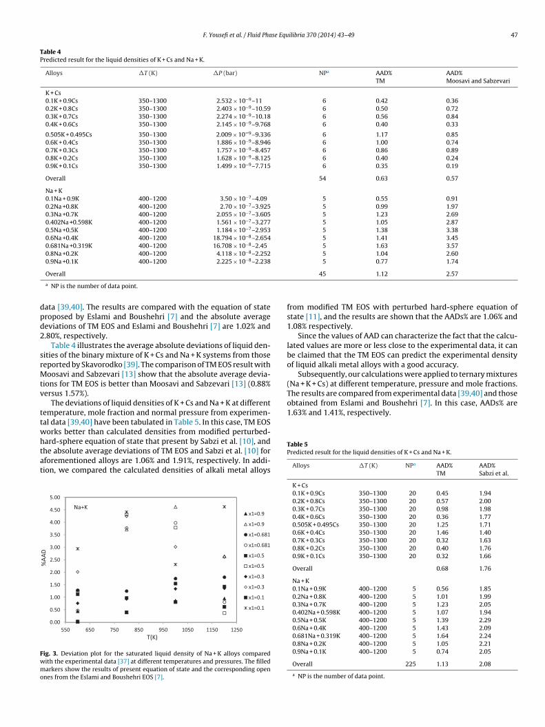
The results are compared from experimental data [39,40] and thoseobtained from Eslami and Boushehri [7]. In this case, AADs% are1.63% and 1.41%, respectively.

Overall

a NP is the number of data point.

ata [39,40]. The results are compared with the equation of stateroposed by Eslami and Boushehri [7] and the absolute averageeviations of TM EOS and Eslami and Boushehri [7] are 1.02% and.80%, respectively.

Table 4 illustrates the average absolute deviations of liquid den-ities of the binary mixture of K + Cs and Na + K systems from thoseeported by Skavorodko [39]. The comparison of TM EOS result withoosavi and Sabzevari [13] show that the absolute average devia-

ions for TM EOS is better than Moosavi and Sabzevari [13] (0.88%ersus 1.57%).

The deviations of liquid densities of K + Cs and Na + K at differentemperature, mole fraction and normal pressure from experimen-al data [39,40] have been tabulated in Table 5. In this case, TM EOSorks better than calculated densities from modified perturbed-ard-sphere equation of state that present by Sabzi et al. [10], and

he absolute average deviations of TM EOS and Sabzi et al. [10] forforementioned alloys are 1.06% and 1.91%, respectively. In addi-ion, we compared the calculated densities of alkali metal alloys

0.00

0.50

1.00

1.50

2.00

2.50

3.00

3.50

4.00

4.50

5.00

550 65 0 75 0 85 0 95 0 105 0 115 0 125 0

x1=0.9

x1=0.9

x1=0.68 1

x1=0.68 1

x1=0.5

x1=0.5

x1=0.3

x1=0.3

x1=0.1

x1=0.1

%AA

D

T(K)

Na+K

ig. 3. Deviation plot for the saturated liquid density of Na + K alloys comparedith the experimental data [37] at different temperatures and pressures. The filledarkers show the results of present equation of state and the corresponding open

nes from the Eslami and Boushehri EOS [7].

45 1.12 2.57

from modified TM EOS with perturbed hard-sphere equation ofstate [11], and the results are shown that the AADs% are 1.06% and1.08% respectively.

Since the values of AAD can characterize the fact that the calcu-lated values are more or less close to the experimental data, it canbe claimed that the TM EOS can predict the experimental densityof liquid alkali metal alloys with a good accuracy.

Subsequently, our calculations were applied to ternary mixtures(Na + K + Cs) at different temperature, pressure and mole fractions.

Table 5Predicted result for the liquid densities of K + Cs and Na + K.

Alloys T (K) NPa AAD%TM

AAD%Sabzi et al.

K + Cs0.1K + 0.9Cs 350–1300 20 0.45 1.940.2K + 0.8Cs 350–1300 20 0.57 2.000.3K + 0.7Cs 350–1300 20 0.98 1.980.4K + 0.6Cs 350–1300 20 0.36 1.770.505K + 0.495Cs 350–1300 20 1.25 1.710.6K + 0.4Cs 350–1300 20 1.46 1.400.7K + 0.3Cs 350–1300 20 0.32 1.630.8K + 0.2Cs 350–1300 20 0.40 1.760.9K + 0.1Cs 350–1300 20 0.32 1.66

Overall 0.68 1.76

Na + K0.1Na + 0.9K 400–1200 5 0.56 1.850.2Na + 0.8K 400–1200 5 1.01 1.990.3Na + 0.7K 400–1200 5 1.23 2.050.402Na + 0.598K 400–1200 5 1.07 1.940.5Na + 0.5K 400–1200 5 1.39 2.290.6Na + 0.4K 400–1200 5 1.43 2.090.681Na + 0.319K 400–1200 5 1.64 2.240.8Na + 0.2K 400–1200 5 1.05 2.210.9Na + 0.1K 400–1200 5 0.74 2.05

Overall 225 1.13 2.08

a NP is the number of data point.

48 F. Yousefi et al. / Fluid Phase Equilibria 370 (2014) 43–49

6

11

16

21

26

31

36

6 11 16 21 26 31 36

Pred

icte

d D

ensit

y(m

ol/L

)

Experiment al De nsit y(mol/ L)

6

11

16

21

26

31

36

6 11 16 21 26 31 36

Pred

icte

d D

ensit

y(m

ol/L

)

Experiment al De nsit y(mol/ L)

6

11

16

21

26

31

36

6 11 16 21 26 31 36

Pred

icte

d D

ensit

y(m

ol/L

)

Experiment al De nsit y(mol/ L)

a b

c

F alloysa

mS[

v(ofiio

TT

ig. 4. Modeling ability of the optimized ANN to predicate of densities of alkali metalnd R2 = 0.996), (c) validating data (AAD% = 0.25 and R2 = 0.999).

Also, the calculated densities from TM EOS for all liquid alkalietal alloys (Na + K, K + Cs and Na + K + Cs) are compared with PC-

AFT equation of state and their AADs% from experimental data40] are 1.14% and 2.23%, respectively.

Also, the MLP was described prior (see Section 2) was trained,alidated and tested with randomly 65% (333 data points), 10%128 data points), and the 25% (51 data points) respectively. The

btained results based on the trial and error procedure leads tond the optimum parameters including the number of the neurons

n the hidden layer, and neurons weights connectivity. The resultsf the obtained AAD% and R2 values for the different numbers of

able 6he performance analyses of different ANN topology.

Hidden neurons Error analysis

AAD% R2

Train Test Train Test

1 6.046 7.338 0.911 0.9102 0.787 0.998 0.950 0.9633 0.666 0.678 0.954 0.9714 0.489 0.600 0.969 0.9755 0.449 0.462 0.975 0.9836 0.424 0.451 0978 0.9887 0.4518 0.455 0.971 0.9868 0.467 0.472 0.974 0.9849 0.346 0.240 0.987 0.992

10 0.229 0.222 0.994 0.99611 0.327 0.264 0.995 0.99512 0.298 0.262 0.974 0.99413 0.373 0.516 0.971 0.99414 0.294 0.362 0.960 0.99515 0.387 0.382 0.980 0.993

based on: (a) training data (AAD% = 0.23 and R2 = 0.995), (b) testing data (AAD% = 0.22

the neurons were given in Table 6. The statistical error analysis inTable 6 showed that the best number of neurons in the hidden layeris 10 which lead to the lowest AAD% for both training and testingsubsets

The obtained results which were given in Fig. 4a show a goodcapability of the trained network to calculate the molar density ofmixtures. The error analysis including AAD% (0.229%) and R2 value(0.994) for the training show the adequate precision of the pro-posed model. Also, the trained network was tested and validatedusing the experimental data points which were not considered inthe training stage. The results shown from Fig. 4b and c includingerror analysis of testing data (AAD% = 0.299 and R2 = 0.996) and val-idating data (AAD% = 0.250 and R2 = 0.999) respectively, confirm thegood ability of the proposed network to predict and generalized ofmolar density over all available experimental data points. It shouldbe stated that the software which used to ANN model is Matlabsoftware.

4. Conclusions

In this research, the modified TM equations of state were used topredict the volumetric properties and thermodynamic properties ofpure liquid alkali metals and their alloys in different temperatures,pressures and mole fractions. The obtained mean of the deviationsfor all pure alkali metals and their alloys were 0.35% and 1.14%,respectively. The ability of TM EOS and ANN for estimation of PVTxof mentioned alkali metals alloys was checked. The results showed

that an ANN with optimum topology (4-10-1neroun) have goodaccuracy (AAD% = 0.299) and correlation coefficient (R2 = 0.996) toestimate density of liquid alkali metals. The result shows that ANNis a proficient method with better accuracy.

se Equ

A

t

R

[

[

[

[[[

[[[[

[

[

[[[

[

[[

[

[

[

[[[[

[

[

[

[331–340.

F. Yousefi et al. / Fluid Pha

cknowledgement

The authors would like to thank Yasouj University for supportinghis project.

eferences

[1] R.D. Kale, M. Rajan, Current Science 86 (2004) 668–675.[2] H.U. Borgstedt, C. Guminski, Monatshefte Fur Chemie 131 (2000) 917–930.[3] F. Hensel, Journal of Non-Crystaline solids 1 (2002) 312–314.[4] H. Eslami, Journal of Nuclear Materials 336 (2005) 135–139.[5] E.K. Goharshadi, A.R. Berenji, Journal of Nuclear Materials 348 (2006) 40–44.[6] M.H. Mousazadeh, M. Ghanadi Marageh, Journal of Physics: Condensed Matter

18 (2006) 4793–4800.[7] H. Eslami, A. Boushehri, Fluid Phase Equilibria 152 (1998) 235–242.[8] H. Eslami, International Journal of Thermophysics 20 (1998) 1575–1585.[9] L. Maftoon-Azad, H. Eslami, A. Boushehri, Fluid Phase Equilibria 263 (2008) 1–5.10] F. Sabzi, H. Eslami, A. Boushehri, Journal of Non-Crystaline solids 352 (2006)

3113–3120.11] F. Mozaffari, H. Eslami, A. Boushehri, International Journal of Thermophysics

28 (2007) 1–8.12] M.H. Mousazadeh, E. Faramarzi, Z. Maleki, Thermochimica Acta 511 (2010)

147–151.13] M. Moosavi, S. Sabzevari, Journal of Molecular Liquids 174 (2012) 117–126.14] M. Moosavi, S. Sabzevari, Fluid Phase Equilibria 329 (2012) 63–70.15] F. Yousefi, H. Karimi, Journal of Industrial and Engineering Chemistry 19 (2013)

498–507.16] J.A. Lazzus, J. Taiwan, Institution of Chemical Engineers 40 (2009) 213–232.17] H. Karimi, F. Yousefi, Fluid Phase Equilibria 336 (2012) 79–83.

18] F.M. Tao, E.A. Mason, Journal of Chemical Physics 100 (1994) 9075–9084.19] F. Yousefi, J. Moghadasi, M.M. Papari, A. Campo, Industrial and Engineering

Chemistry Research 48 (2009) 5079–5084.20] H. Karimi, F. Yousefi, M.M. Papari, Journal of Chemistry and Engineering of Japan

44 (2011) 295–303.

[

[

ilibria 370 (2014) 43–49 49

21] H. Karimi, F. Yousefi, M.M. Papari, Chinese Journal of Chemical Engineering 19(2011) 496–503.

22] F. Yousefi, H. Karimi, Ionics 18 (2012) 135–142.23] F. Yousefi, H. Karimi, European Polymer Journal 48 (2012) 1135–1143.24] Z. Zhang, K. Fried, Composites Science and Technology 63 (2003) 2029–

2036.25] A. Khajeh, H. Modarress, Expert Systems with Applications 37 (2010)

3070–3074.26] F. Gharagheizi, G.R. Salehib, Thermochimica Acta 521 (2011) 37–40.27] A. Sencan, I. Ilke Köse, R. Selbas, Energy Conversion and Management 52 (2011)

958–974.28] J.M.H. Levelt Sengers, U.K. Deiters, U. Klask, P. Swidersky, G.M. Schneider, Inter-

national Journal of Thermophysics 14 (1993) 893–922.29] S.I. Sandler, Chemical and Engineering Thermophysics, Wiley, New York,

1989.30] J.M. Prauznitz, R.N. Lichtentaler, E.G. Azevedo, Molecular Thermodynamics of

Fluid Phase Equilibria, Prentice-Hall, Englewood Cliffs, NJ, 1999.31] G. Ihm, Y. Song, E.A. Mason, Fluid Phase Equilibria 75 (1992) 117–125.32] C. Tsonopolous, AIChE Journal 24 (1978) 1112–1127.33] H. Eslami, International Journal of Thermophysics 21 (2000) 1123–1136.34] C. Bishop, Neural networks for pattern recognition, Oxford Clarendon, Oxford,

1996.35] B. Ripley, Pattern Recognition and Neural Networks, Cambridge University

Press, Cambridge, 1996.36] C.A. Nieto de Castro, J.M.N.A. Fareleira, P.M. Matias, M.L.V. Ramires, A.A.C.

Canelas, A.J.C. Varandas, Berichte der Bunsengesellschaft für physikalischeChemie 74 (1990) 53–58.

37] N.B. Vargaftik, Handbook of Physical Properties of Liquids and Gases, 2nd ed.,Hemisphere, Washington, DC, 1983.

38] N. Mehdipour, A. Boushehri, International Journal of Thermophysics 19 (1997)

39] S.K. Skavorodko, High Temperature (dissertation), Institute for Acad. Sci., USSR,Moscow, 1980.

40] V.V. Roschupkin, M.A. Pokrasin, A.I. Chernov, High Temperature–High Pressure23 (1990) 697–700.