Epsilon–optimal synthesis for vehicles withvertically bounded Field-Of-View

Paolo Salaris, Andrea Cristofaro, Lucia Pallottino, Antonio Bicchi

Abstract—This paper presents a contribution to the problem ofobtaining an optimal synthesis for shortest paths for a unicycleguided by an on–board limited Field–Of–View (FOV) sensor,which must keep a given landmark in sight. Previous workson this subject have provided an optimal synthesis for the casein which the FOV is limited in the horizontal directions (H–FOV, i.e. left and right boundaries). In this paper we study thecomplementary case in which the FOV is limited only in thevertical direction (V–FOV, i.e. upper and lower boundaries). Withrespect to the H–FOV case, the vertical limitation is all but asimple extension. Indeed, not only the geometry of extremal arcsis different, but also a more complex structure of the synthesis isrevealed by analysis. We will indeed show that there exist initialconfigurations for which the optimal path does not exist. In suchcases, we provide an e–optimal path whose length approximatesarbitrarily well any other shorter path. Finally, we provide apartition of the motion plane in regions such that the optimalor e–optimal path from each point in that region is univocallydetermined.

I. INTRODUCTION

The final goal of the proposed research is to study theproblem of maintaining visibility of a set of landmarks with anonholonomic vehicle equipped with a limited Field–Of–View(FOV) sensor. A preliminary analysis on local optimal paths,in case of a set of landmarks and considering a FOV withhorizontal bounds, can be found in [1] where a randomizedplanner is also proposed. To the authors’ best knowledge, noresults have already been obtained for a FOV with verticalbounds. Hence, in this paper we consider the simplified caseof a single landmark determining global optimal paths for avertically limited FOV. In other words, the goal is to obtainshortest paths from any point on the motion plane to a desiredposition while keeping, along the path, a given landmark withinthe vertical bounds of the camera.

Regarding optimal (shortest) paths in absence of sensorconstraints, the seminal work on unicycle vehicles [2] providesa characterization of shortest curves for a car with a boundedturning radius. In [3], authors determine a complete finitepartition of the motion plane in regions characterizing theshortest path from all points in the same region, i.e. a synthesis.A similar problem with the car moving both forward andbackward has been solved in [4] and refined in [5]. The global

This work was supported by E.C. contracts n.224053 CONET (CooperatingObjects Network of Excellence), n. 257462 HYCON2 (Network of Excellence)and n.2577649 PLANET.

Salaris, Pallottino and Bicchi are with the Research Center “Enrico Piaggio”and Dipartimento di Ingegneria dell’Informazione, University of Pisa, Italy.Bicchi is also with the Department of Advanced Robotics, Istituto Italianodi Tecnologia, Genova, Italy. Cristofaro is with the School of Science andTechnology, University of Camerino, Italy.

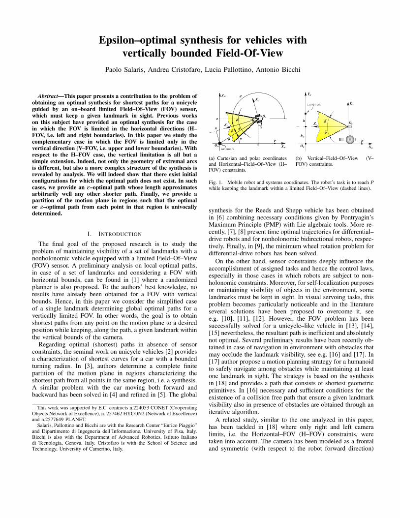
(a) Cartesian and polar coordinatesand Horizontal–Field–Of–View (H–FOV) constraints.

(b) Vertical–Field–Of–View (V–FOV) constraints.

Fig. 1. Mobile robot and systems coordinates. The robot’s task is to reach Pwhile keeping the landmark within a limited Field–Of–View (dashed lines).

synthesis for the Reeds and Shepp vehicle has been obtainedin [6] combining necessary conditions given by Pontryagin’sMaximum Principle (PMP) with Lie algebraic tools. More re-cently, [7], [8] present time optimal trajectories for differential–drive robots and for nonholonomic bidirectional robots, respec-tively. Finally, in [9], the minimum wheel rotation problem fordifferential-drive robots has been solved.

On the other hand, sensor constraints deeply influence theaccomplishment of assigned tasks and hence the control laws,especially in those cases in which robots are subject to non-holonomic constraints. Moreover, for self-localization purposesor maintaining visibility of objects in the environment, somelandmarks must be kept in sight. In visual servoing tasks, thisproblem becomes particularly noticeable and in the literatureseveral solutions have been proposed to overcome it, seee.g. [10], [11], [12]. However, the FOV problem has beensuccessfully solved for a unicycle–like vehicle in [13], [14],[15] nevertheless, the resultant path is inefficient and absolutelynot optimal. Several preliminary results have been recently ob-tained in case of navigation in environment with obstacles thatmay occlude the landmark visibility, see e.g. [16] and [17]. In[17] author propose a motion planning strategy for a humanoidto safely navigate among obstacles while maintaining at leastone landmark in sight. The strategy is based on the synthesisin [18] and provides a path that consists of shortest geometricprimitives. In [16] necessary and sufficient conditions for theexistence of a collision free path that ensure a given landmarkvisibility also in presence of obstacles are obtained through aniterative algorithm.

A related study, similar to the one analyzed in this paper,has been tackled in [18] where only right and left cameralimits, i.e. the Horizontal–FOV (H–FOV) constraints, weretaken into account. The camera has been modeled as a frontaland symmetric (with respect to the robot forward direction)

Fig. 2. Sensor model: four-sided right rectangular pyramid.

planar cone, as represented in Fig. 1(a). The constraint onthe symmetry (with respect to the robot forward direction)of the planar cone has been relaxed in [19] where the robotforward direction is not necessarily supposed to be includedinside the planar cone. After showing that logarithmic spirals,straight lines and rotations on the spot are extremal arcs of theoptimal control problem, a finite alphabet of these arcs hasbeen obtained and the shortest paths from any point on themotion plane to a desired final configuration, i.e. a synthesis,has been provided. In [20], based on the geometric propertiesof the synthesis proposed in [18], optimal feedback controllaws which are able to align the vehicle to the shortest pathfrom the current configuration are also defined, for any pointon the motion plane. Moreover, based on the same synthesis,a switched, homography–based, visual servoing scheme isproposed in [21] to steer the vehicle along the optimal paths.

However, in real cameras there exist also the upper andlower limits that previous works have not taken into account.Hence, in this work we study the complementary case in whichonly upper and lower camera limits are considered, i.e. theVertical–FOV (V–FOV) constraints, see Fig. 1(b). The goalof our research is to obtain first the optimal paths takinginto account both kinematics and V–FOV constraints and thenthe optimal synthesis of the motion plane. Finally, from theoptimal synthesis, optimal feedback control laws might bederived to steer the vehicle toward the goal without violatingthe constraints. Once the synthesis of this problem is obtained,the optimal synthesis for a realistic sensor modeled as a four–sided right rectangular pyramid (see Fig. 2), can be achievedby appropriately merging synthesis provided in [18] with thatprovided in this paper.

In this work, we first show that involutes of circle, straightlines and rotations on the spot are extremal arcs of the V–FOV problem, and then we exploit geometric properties ofthese arcs to achieve the synthesis. However, several aspectsmake the problem addressed in this paper much more difficultwith respect to the one in [18] and prevent us to use thesame approach to tackle the problem. One is that there existsa compact set around the feature for which paths reachingit now become impracticable since they violate the V–FOVconstraints. Moreover, the whole procedure adopted in [18] forobtaining the final synthesis is mainly based on the invariance

property of logarithmic spirals with respect to scaling (withcenter at the origin). Unfortunately, involutes of circle do nothave this property and hence a different approach must beused. Moreover, a major challenge is that, for the V–FOV case,there exist points in the motion plane from which the optimalpath does not exist. Indeed, the paths would consist of infinitesequences of arcs whose total lengths are anyhow proved tobe finite. On the other hand, an e–optimal path whose lengthapproximates arbitrarily well any other shorter path can bedetermined and used to obtain an e–optimal synthesis.

Preliminary results on this problem have been publishedin [22] where, for space limitations, several proofs and tech-nical details have been omitted. In this paper we briefly reportthe results in [22] necessary for the characterization of theoptimal synthesis together with the missing proofs. From theresults in [22] we will characterize the optimal and e–optimalpaths with respect to the relative positions of initial and finalpoints. Finally, we will provide the main contribution of thepaper that is the subdivision of the motion plane in regions ofpoints that are characterized by the same optimal or e–optimalpath typology, i.e. the e–optimal synthesis.

It is worth noticing that the results obtained in this paperare necessary to determine the optimal synthesis for a FOVwith both horizontal and vertical limits. This can be done byintegrating, with a non straightforward procedure, the obtainedsynthesis with the one in [18]. Thus, the complete synthesiscould be extended to the multi-feature case with the resultsin [1].

As in previous works, in this paper a fixed on–board camerais considered. There are multiple reasons for our focus on suchcameras, of both a technological and a theoretical nature.

From a technological point of view, although pan–tilt cam-eras costs are not prohibitive, they remain much more complexand prone to failures. Furthermore, angle measurement errorsand backlash in the mechanism may add significantly to local-ization errors. From a functional viewpoint, having a panningmechanism effectively widens the H–FOV by the angular rangespanned by the camera motor; similarly, the tilting mechanismwidens the V–FOV, which is the issue relevant to this paper. Ifthe pan and tilt angles are wide enough to cover the whole 4p

solid angle, then optimal control is trivialized to a non-limitedFOV problem. If otherwise the pan/tilt angles are limited (suchas e.g. in [16], [1], [17] and [21]), then our problem definitionremains valid, only with wider bounds.

From a theoretical point of view, however, our analysisworks in the assumption that the camera plane is orthogonalto the motion plane. The control extremals and the synthesisfor different tilting angles needs a specific analysis. Moreover,if the tilting angle is changed along the motion, a wholly newoptimal control problem with three instead of two inputs isgenerated. The study of this problem is not considered in thispaper.

II. PROBLEM DEFINITION

Consider a vehicle moving on a plane where a right-handedreference frame hW i is defined with origin in Ow and axesXw,Zw. The configuration of the vehicle is described by x (t) =

(x(t),z(t),q(t)), where (x(t),z(t)) is the position in hW i of areference point in the vehicle, and q(t) is the vehicle headingwith respect to the Xw axis (see Fig. 1). We assume that thedynamics of the vehicle are negligible, and that the forward andangular velocities, n(t) and w(t) respectively, are the controlinputs of the kinematic model of the vehicle. Choosing polarcoordinates (see Fig. 1), the kinematic model of the unicycle-like robot is

2

4r

y

b

3

5=

2

64�cosb 0

sinb

r

0sinb

r

�1

3

75

n

w

�. (1)

We consider vehicles with bounded velocities which can turnon the spot. In other words, we assume

(n ,w) 2U, (2)

where U is a compact and convex subset of IR2, containingthe origin in its interior.

The vehicle is equipped with a rigidly fixed pinhole camerawith a reference frame hCi = {Oc,Xc,Yc,Zc} such that theoptical center Oc corresponds to the robot’s center [x(t),z(t)]Tand the optical axis Zc is aligned with the robot’s forwarddirection. Cameras can be generically modeled as a four-sidedright rectangular pyramid, as shown in Fig. 2. Its characteristicsolid angle is given by W = 4arcsin

�sin f sinf

�and e = 2f

and d = 2f are the apex angles, i.e. dihedral angles measuredto the opposite side faces of the pyramid. We will refer tothose angles as the vertical and horizontal angular aperture ofthe sensor, respectively. Moreover, f is half of the V–FOVangular aperture, whereas f is half of the H–FOV angularaperture.

In [18], authors have provided a complete characterizationof shortest paths towards a goal point taking into account onlya limited horizontal aperture of the camera and hence modelingthe camera FOV as a planar cone moving with the robot. Theobtained optimal paths consist of at most 5 arcs of three types:rotations on the spot (denoted by the symbol ⇤), straight lines(S) and left and right logarithmic spirals (T L and T R). Finallyan optimal synthesis has been obtained, i.e. a subdivision ofthe motion plane in regions such that an optimal sequenceof symbols (corresponding to an optimal path) is univocallyassociated to a region and completely describes the shortestpath from each point in that region to the desired goal.

In this paper, we consider only the upper and lower limitsof the camera, i.e. we assume f = p/2. Moreover, we considerthe most interesting case in which f is less than p/2. The goalis hence to obtain the optimal synthesis considering only theV–FOV constraints.

Without loss of generality, the feature to be kept within thevertically limited FOV lays on the axis through the origin Ow,perpendicular to the motion plane (see Fig. 1). Referring toFig. 2, h+hc and h are the feature heights from Ow and fromthe plane Xc⇥Zc respectively. We denote with (r, y)= (rP, 0)the position, on the Xw axis, of the robot target point P.

Remark 1: In order to maintain the feature within the ver-

tical FOV, the following must hold:

r cosb � htan f

= Rb . (3)

Indeed, considering a pinhole camera model [23], the positionof the landmark in the image plane is given by

Ix = fcxcz

, (4)

Iy = fhcz, (5)

where cx = r sinb and cz = r cosb are the coordinates of thelandmark in the camera frame hCi and f is the focal length,i.e. OcOI (see Fig. 2). Since the vehicle is moving on a plane,a constant value of Iy corresponds to a constant cz = r cosb ,see Fig. 1(a). The maximum allowable value for Iy depends onthe vertical angular aperture of the camera, hence Iy f tan f .Finally, substituting cz = r cosb in (5) we obtain (3).

Definition 1: Let Z0 = {(r, y)|r <Rb} be the disk centeredin the origin with radius Rb and Z1 = {(r, y)|r � Rb}.

Remark 2: Z0 is the set of points in IR2 that violates theV–FOV constraint (3) for any value of the bearing angle b .Notice that points with r = Rb verify the constraint only ifb = 0. Z1 is the set of points in IR2 such that inequality (3)holds.

To determine the motion plane synthesis, we are nowinterested in studying the shortest path covered by the center ofthe vehicle from any point Q 2 Z1 to P, such that the feature iskept in the sensor V–FOV. Hence, the problem is to minimizethe cost functional

L =Z

t

0|n |dt , (6)

under the feasibility constraints (2), (3) and the kinematicmodel (1). Since the cost functional (6) does not weight b

the maneuvers consisting of rotations on the spot have zerolength. In the following, these zero cost maneuvers, denotedby ⇤, will be used only to properly connect other maneuvers,i.e. denoting a non smooth transition.

This problem has been preliminary addressed in [22] wherethe first step of the characterization of the shortest paths havebeen considered. However, for space limitations several proofsand results have been omitted. For the sake of clarity andreader convenience, notations, definitions and main results(without proofs) of [22] that are necessary to fully understandthe analysis toward the optimal synthesis of the V–FOV,provided in this paper, will be reported.

III. EXTREMALS AND OPTIMAL CONCATENATIONS

In this section we briefly characterize the extremals of theoptimal control problem, their main geometrical peculiaritiesand their concatenations that can not be part of optimal paths.Moreover, conditions under which such optimal paths do notexist will also be determined. For those purposes, we startanalyzing the V–FOV constraints and the properties of thegeometrical curves followed by the vehicle while movingactivating the constraints.

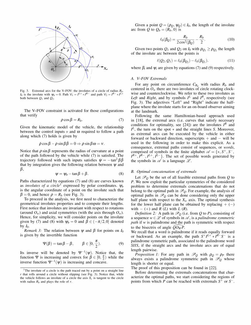
Fig. 3. Extremal arcs for the V–FOV: the involutes of a circle of radius Rb.I0 is the involute with yb = 0. Path C1 = IL+ ⇤ IR� and path C2 = IR� ⇤ IL+

both between Q1 and Q2.

The V–FOV constraint is activated for those configurationsthat verify

r cosb = Rb. (7)

Given the kinematic model of the vehicle, the relationshipbetween the control inputs v and w required to follow a pathalong which (7) holds is given by

r cosb �r sinbb = 0 ) r sinbw = n .

Notice that r sinb represents the radius of curvature at a pointof the path followed by the vehicle while (7) is satisfied. Thetrajectory followed with such inputs satisfies y = � tan2

bb

that by integration gives the following relation between y andb ,

y = yb � tanb +b . (8)

Paths characterized by equations (7) and (8) are curves knownas involutes of a circle1 expressed by polar coordinates. ybis the angular coordinate of a point on the involute such thatb = 0, and hence r = Rb (see Fig. 3).

To proceed in the analysis, we first need to characterize thegeometrical involutes properties and to compute their lengths.First notice that involutes are invariant with respect to rotations(around Ow) and axial symmetries (with the axis through Ow).Hence, for simplicity, we will consider points on the involutegiven by (7) and (8) with yb = 0 and b 2 (�p/2,0] denotedby I0.

Remark 3: The relation between y and b for points on I0is given by the invertible function

Y(b ) = tanb �b , b 2 [0,p

2). (9)

Its inverse will be denoted by Y�1(y). Notice that, thefunction Y is increasing and convex for b 2 [0, p

2 ) while theinverse function Y�1(y) is increasing and concave.

1The involute of a circle is the path traced out by a point on a straight liner that rolls around a circle without slipping (see Fig. 3). Notice that, whilethe vehicle follows an involute of a circle the axis Xc is tangent to the circlewith radius Rb and plays the role of r.

Given a point Q = (rQ, yQ) 2 I0, the length of the involutearc from Q to Qb = (Rb, 0) is

`0(bQ) =Rb

2cos2(bQ)� Rb

2. (10)

Given two points Q1 and Q2 on I0 with rQ1 � rQ2 the lengthof the involute arc between the points is

`(Q2,Q1) = `0(bQ2)� `0(bQ1). (11)

where bi and yi are given by equations (7) and (9) respectively.

A. V–FOV ExtremalsFor any point on circumference CRb with radius Rb and

centered in Ow there are two involutes of circle rotating clock-wise and counterclockwise. We refer to these two involutes asLeft and Right, and by symbols IL and IR, respectively (seeFig. 3). The adjectives “Left” and “Right” indicate the half-plane where the involute starts for an on-board observer aimingat the landmark.

Following the same Hamiltonian-based approach usedin [18], the extremal arcs (i.e. curves that satisfy necessaryconditions for optimality, see [24]) are the involutes IR andIL, the turn on the spot ⇤ and the straight lines S. Moreover,as extremal arcs can be executed by the vehicle in eitherforward or backward direction, superscripts + and � will beused in the following in order to make this explicit. As aconsequence, extremal paths consist of sequences, or words,comprised of symbols in the finite alphabet A = {⇤, S+, S�,IR+, IR�, IL+, IL�}. The set of possible words generated bythe symbols in A is a language L .

B. Optimal concatenation of extremalsLet PQ be the set of all feasible extremal paths from Q to

P. We now exploit the particular symmetries of the consideredproblem to determine extremals concatenations that do notbelong to the optimal path in PQ. For example, the analysis ofoptimal paths in PQ can be done considering only the upperhalf plane with respect to the Xw axis. The optimal synthesisfor the lower half plane can be obtained by replacing + (�)with � (+) and R (L) with L (R).

Definition 2: A path in PQ (i.e. from Q to P), consisting ofa sequence w2L of symbols in A , is a palindrome symmetricpath if w is palindrome and the path is symmetric with respectto the bisectrix of angle \QOW P.We recall that a word is palindrome if it reads equally forwardor backward. As an example, the path S+IL+ ⇤ IR�S� is apalindrome symmetric path, associated to the palindrome wordSIIS, if the straight arcs and the involute arcs are of equallength pairwise.

Proposition 1: For any path in PQ with rQ = rP therealways exists a palindrome symmetric path in PQ whoselength is shorter or equal.The proof of this proposition can be found in [22].

Before determining the extremals concatenations that char-acterize the optimal paths, we start considering the regions ofpoints from which P can be reached with extremals S+ or S�.

Fig. 4. Region LimQ with its border ∂LimQ = LimRQ [LimL

Q and cone LQdelimited by half–lines sR

Q and sLQ.

We will show such regions are closed with borders describedby half–lines and curves known as Pascal’s Limacons, [25]

Definition 3: For a point Q 2 IR2, LimRQ (LimL

Q) denotes thearc of the Pascal’s Limacon from Q to O such that, 8V 2 LimR

Q

(LimLQ), \QVOw = p � b , with b = arctan

⇣rQRb sinb

⌘, in the

half-plane on the right (left) of QOw (cf. Fig. 4). Also, letLimQ be the region with borders LimR

Q and LimLQ from Q to

O.Definition 4: For a point Q 2 IR2, sR

Q (sLQ) denotes the half-

line from Q forming an angle yQ + b (yQ � b ), where b =

arccos⇣

RbrQ

⌘, with the Xw axis (cf. Fig. 4). Also, let LQ be the

cone delimited by sRQ and sL

Q.Proposition 2: For any starting point Q, all points of LimQ

(LQ) are reachable by a forward (backward) straight pathwithout violating the V–FOV constraints.The proof of Proposition 2 (that has been omitted in [22] forspace limitations), is based on how the projection on the imageplane of the landmark moves within the sensor limits (see [26])when vehicle performs extremal maneuvers and is reported inAppendix A.

At this point the regions associated to the single straight linemaneuvers have been obtained. Following a similar approachto the one used in [18], the goal is to obtain a sufficientfamily of optimal paths from which the complete synthesiscan be obtained. Unfortunately, in this case optimal paths donot always exist as stated in the following theorem.

Theorem 1: For any Q on the upper half plane, one of thefollowing conditions is verified.

1) There exists a shortest path toward P of type S+IL+ ⇤IR�S� or IR� ⇤ IL+ (or degenerate cases, with sub–pathsof zero length, e.g. S+ ⇤S�).

2) The infimum of the cost functional L is not reached andhence the shortest path does not exist.

In order to prove Theorem 1 we proceed showing that partic-ular extremals concatenations can not belong to any optimal

Fig. 5. Path of type S�Q2⇤ S+Q1

from Q2 = (r,y2) to Q1 = (r,y1) withy2 > y1 can be shortened by a path of type IR�

Q2⇤ IL+

Q1(see Proposition 3).

path. In [22] some results have been obtained in this directionand are summarized in the following Remark for readerconvenience.

Remark 4: For symmetry properties, it is sufficient to con-sider a starting point Q = (rQ,yQ) with yQ � 0. From suchQ the optimal path toward P lays on the upper half-plane andarcs of type IR+ and IL� are not part of the optimal path.Moreover, in the optimal paths the arc S� can not be followedby arcs of type IR� and IL+ while arc S+ can not follow arcsof type IL+ and IR�.

Those results can be further refined with the followingproposition that excludes concatenations of type S� ⇤S+ fromoptimal paths.

Proposition 3: Any path of type S� ⇤ S+ between Q1 =(r,y1) and Q2 = (r,y2) with y2 > y1 can be shortened by apath of type IR� ⇤ IL+.

Proof: Referring to Fig. 5, let N1 be the switching pointbetween arcs S� and S+. From Proposition 2 we have thatN1 2 LQ2 \LQ1 . However, among all paths of type S� ⇤ S+,the shortest one has N1 2 ∂LQ2 \ ∂LQ1 . In this case, fromDefinition 4, IR�

Q2is tangent to S� in Q2 and IL+

Q1is tangent to

S+ in Q1. Moreover, the path IR� ⇤ IL+ lays between S� ⇤S+and Q1Q2. For the convexity of both paths, the length of S� ⇤S+ is longer than the length of IR� ⇤ IL+ and hence the thesis.

Extremals can be represented by nodes of a graph whilepossible concatenation by arrows where an arc with (⇤)denotes a non smooth concatenation. The graph reported inFig. 6 represent a graphical summary of the results obtainedso far. The obtained graph is not acyclic and hence optimal

Fig. 6. Extremals and sequences of extremals from points IR2.

path consisting of infinite number of extremals are, at this

point, neither excluded nor proved. Hence, to conclude theanalysis of optimal extremal concatenations we need to studyconcatenations of type IL+ ⇤ IR� and IR� ⇤ IL+.

IV. INFINITE SEQUENCES OF INVOLUTE ARCS

In this section we will show that the particular characteristicsof the involute arcs may give rise to an infimum (and finite) arclength consisting of infinite involutes of infinitesimal length.To study the occurrence of such peculiarity, we considerQ1 = (rQ1 ,yQ1) and Q2 = (rQ2 ,yQ2) with rQ1 = rQ2 andyQ1 > yQ2 . The points Q1 and Q2 can be connected bytwo paths, each one palindrome and hence symmetric withrespect to the bisectrix of angle \Q1OwQ2, consisting of twopairs of involute curves C1 = IL+ ⇤ IR� and C2 = IR� ⇤ IL+.Let H1 = (rH1 ,yH1) and H2 = (rH2 ,yH2) be the points ofintersection of the involute curves on C1 and C2 respectively,i.e. rH1 < rQi < rH2 and yH1 = yH2 . We denote by L(C1) andL(C2) the lengths of the curves C1 and C2, respectively.

The goal of this section is to prove that the shortest pathconsisting only of involutes, between two points Q1 and Q2 ona circumference, is of type C2 (evolving outside the circum-ference) if rQ1 and the angle \Q1OwQ2 are sufficiently small.On the other hand, it is of type C1 (hence a pair of involuteevolving inside the circumference) if rQ1 is sufficiently largewhile the angle \Q1OwQ2 is sufficiently small. Otherwise, theshortest path consisting only of involutes does not exist. Moreformally, we will prove

Theorem 2: Given the points Q1 = (rQ1 ,yQ1) and Q2 =(rQ2 ,yQ2) with rQ1 = rQ2 and yQ1 > yQ2 . Recalling thatr2 =

p2Rb, it holds that

1) for rQ1 2 [Rb,r2),a) if yQ1 �yQ2 2(Y(p/4)�yQ1) the optimal trajectory

from Q1 to Q2 is C2 = IR� ⇤ IL+.b) yQ1 �yQ2 > 2(Y(p/4)�yQ1) the shortest path does

not exist.2) For rQ1 � r2

a) if yQ1 �yQ2 > 2(yQ1 �Y(p/4)) the shortest path doesnot exist.

b) if yQ1 �yQ2 2(yQ1 �Y(p/4)) the optimal trajectoryfrom Q1 to Q2 is C1 = IL+ ⇤ IR�

The proof of this theorem follows straightforwardly from theresults stated in the following two propositions. In the first oneonly pairs of involutes (C1 and C2) are taken into account whilein the second an arbitrary number of involutes are considered.Hence, we start comparing the lengths L(C1) and L(C2) tocharacterize the conditions on rQ1 and rH1 under which oneis smaller than the other.

Proposition 4: There exist r and r with r > r2 > r suchthat

1) rQ1 r2 ) L(C2) L(C1) 8rH1 .2) rQ1 2 (r2, r), rH1 < r ) L(C2)< L(C1)3) rQ1 2 (r2, r), rH1 > r ) L(C1)< L(C2)4) rQ1 � r ) L(C1) L(C2) 8rH1 .The proof of this proposition, omitted in [22] for brevity,

can be found in Appendix B. The value rH1 of the switching

point H1 with respect to r can be rewritten in terms of theangle yQ1 �yQ2 spanned by C1 and C2 as in the followingproposition where we consider also the possibility of connect-ing Q1 and Q2 with path consisting of an arbitrary number ofinvolutes.

The following Proposition is a collection of results in [22]and provides conditions under which the optimal path does notexist.

Proposition 5: Consider the points Q1 = (rQ1 ,yQ1) andQ2 = (rQ1 ,yQ2) with yQ1 > yQ2 .

1) if rQ1 < r2, and Y(p/4)�yQ1 � yQ1�yQ22 the optimal

trajectory consisting of involutes from Q1 to Q2 is C2 =IR� ⇤ IL+.

2) if rQ1 = r2 and 8yQ2 , the optimal (shortest) path betweenQ1 and Q2 consisting of involutes does not exist, i.e. theinfimum of the cost functional (6) is not reached.

3) If rQ1 > r2, and yQ1 �Y(p/4) � yQ1�yQ22 the optimal

trajectory consisting of involutes from Q1 to Q2 is C1 =IL+ ⇤ IR�.

The proposition states that whenever C1 or C2 intersects thecircumference of radius r2 they can both be shortened. Forexample, if C1 crosses the circumference of radius r2 in G1 andG2 the sub–path between such points can be shortened witha path of type C2 (see Proposition 4 second item). Moreover,from Proposition 4 third item, this shorter path of type C2 canin turn be shortened by a path consisting of two or more sub–paths of type C2. By iterating this procedure it is possible toconclude the non-existence of a shortest path between Q1 andQ2 with rQ1 = rQ2 = r2.

For those cases in which the path does not exist, we arenow interested in the infimum of the lengths of the pathsconsisting of infinite pairs of involutes of type C2. Thefollowing Theorem, whose proof can be found in [22], statesthat such infimum length is finite.

Theorem 3: Consider r = r2, the point Q1 = (r,yQ1) 2 I0and a point Q2 = (r,yQ2) with yQ1 >yQ2 and yQ1 �yQ2 p .The infimum of the lengths of the paths consisting of infinitesub–paths of type C2 from Q1 to Q2 is finite and

Lin f (Q1,Q2) =p

2(r2(yQ1 �yQ2))

i.e.p

2 times the length of the circular arc from Q1 to Q2 onthe circumference with radius r2.

From a practical point of view, the infimum length pathcan be approximated by paths consisting of a finite sequenceof involutes. The approximation error is as smaller as moreaccurate is the wheel motor.

Definition 5: C(n) is the path from Q1 to Q2 on the circum-ference of radius r2 consisting of n identical sub–paths of typeC2, i.e. C(n) = IR� ⇤ IL+ ⇤ IR� ⇤ IL+ ⇤ · · ·⇤ IR� ⇤ IL+ ⇤ IR� ⇤ IL+.

The following corollary provides a sufficient number n ofsub–paths of type C2 in C(n) such that the length of any othershorter path is no longer than an arbitrarily small e > 0.

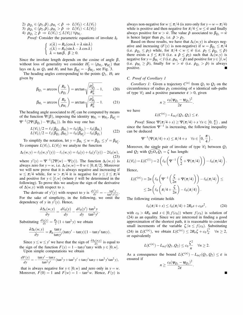
Corollary 1: Given a trajectory C(n) from Q1 to Q2 on thecircumference of radius r2 and a positive parameter e > 0,there exists c0 > 4Rb such that for

n �c0(yQ1 �yQ2)

2

2e

we have L(C(n))�Lin f (Q1,Q2) e.The proof can be found in Appendix C.

From a practical point of view, consider a robot whosemotor accuracy allows it to follow a path of type C2 onthe circumference of radius r2 with amplitudes larger thand . Hence, given points Q1 to Q2 on the circumference ofradius r2, the path of minimum length that can be followedby the robot is C(n) with n = b |yQ2�yQ1 |

d

c whose length can becomputed and compared with Lin f .

Definition 6: Given e > 0, Ze

=C(n(e)) is the path consistingof a sequence of n(e) arcs of type C2 on circumference ofradius r2.

Since the infimum length is finite and there exist arcs of typeZ

e

whose lengths are arbitrarily close to the infimum one, withan abuse of notation we will denote with Z the non existing butapproximable path and we consider Z as a pseudo extremal arc.The alphabet A is extended with Z obtaining a new alphabetAZ . If a path contains the symbol Z we use the analyticalexpression of the path length to determine the infimum lengthpath from any point of the motion plane. Notice that suchpaths are optimal only if they do not contain arcs Z. Witha slight abuse of language sequences associated to infimumlength paths will be referred to as the optimal language onAZ and the induced synthesis will be referred to as optimalsynthesis. True e–optimal synthesis will finally be obtainedsubstituting Z with its e–optimal subpath Z

e

.

V. THE OPTIMAL LANGUAGE

Based on the results of previous sections we are now inter-ested in determining the optimal language that characterizesthe infimum length paths. Based on Theorem 2, it follows thatsequences S+ ⇤ IR� and IL+ ⇤S� do not belong to any infimumlength path. Indeed it holds

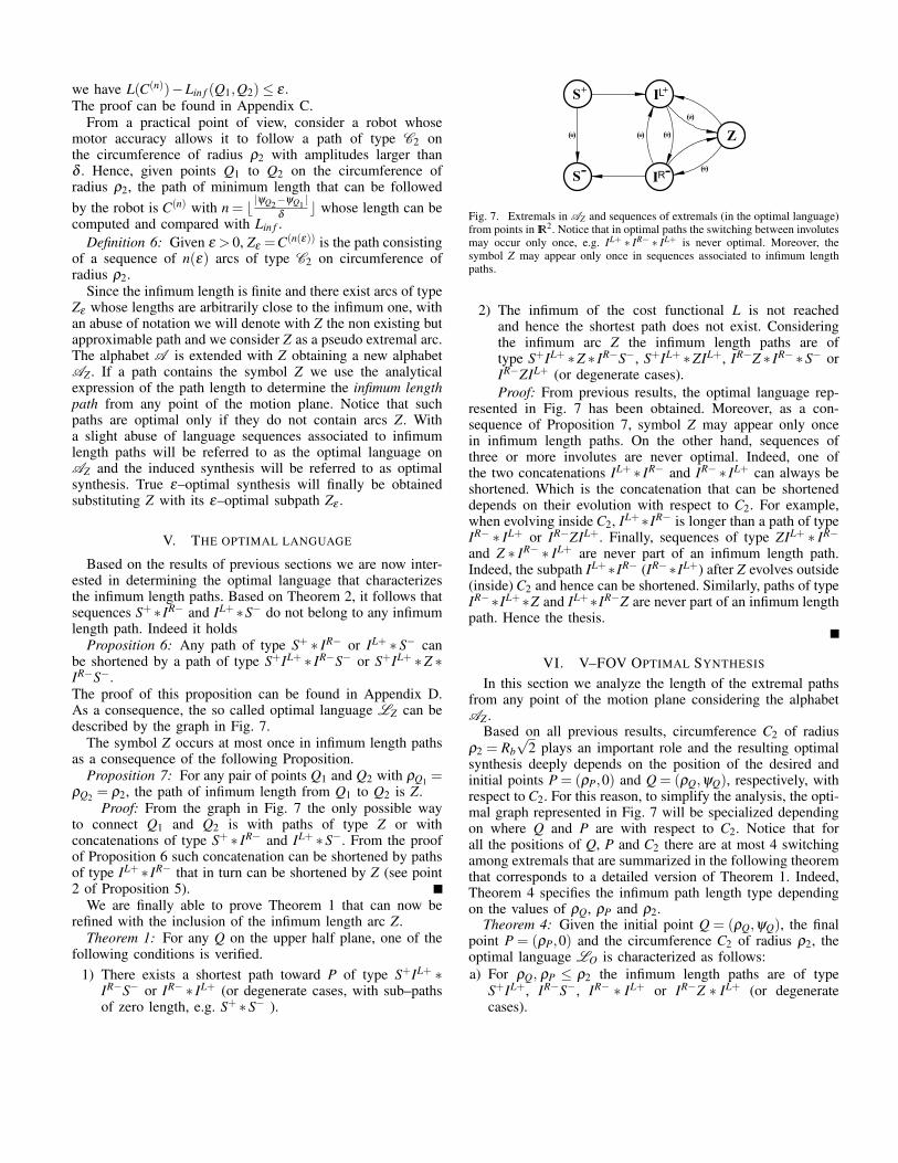
Proposition 6: Any path of type S+ ⇤ IR� or IL+ ⇤ S� canbe shortened by a path of type S+IL+ ⇤ IR�S� or S+IL+ ⇤Z ⇤IR�S�.The proof of this proposition can be found in Appendix D.As a consequence, the so called optimal language LZ can bedescribed by the graph in Fig. 7.

The symbol Z occurs at most once in infimum length pathsas a consequence of the following Proposition.

Proposition 7: For any pair of points Q1 and Q2 with rQ1 =rQ2 = r2, the path of infimum length from Q1 to Q2 is Z.

Proof: From the graph in Fig. 7 the only possible wayto connect Q1 and Q2 is with paths of type Z or withconcatenations of type S+ ⇤ IR� and IL+ ⇤S�. From the proofof Proposition 6 such concatenation can be shortened by pathsof type IL+ ⇤ IR� that in turn can be shortened by Z (see point2 of Proposition 5).

We are finally able to prove Theorem 1 that can now berefined with the inclusion of the infimum length arc Z.

Theorem 1: For any Q on the upper half plane, one of thefollowing conditions is verified.

1) There exists a shortest path toward P of type S+IL+ ⇤IR�S� or IR� ⇤ IL+ (or degenerate cases, with sub–pathsof zero length, e.g. S+ ⇤S� ).

Fig. 7. Extremals in AZ and sequences of extremals (in the optimal language)from points in IR2. Notice that in optimal paths the switching between involutesmay occur only once, e.g. IL+ ⇤ IR� ⇤ IL+ is never optimal. Moreover, thesymbol Z may appear only once in sequences associated to infimum lengthpaths.

2) The infimum of the cost functional L is not reachedand hence the shortest path does not exist. Consideringthe infimum arc Z the infimum length paths are oftype S+IL+ ⇤Z ⇤ IR�S�, S+IL+ ⇤ZIL+, IR�Z ⇤ IR� ⇤S� orIR�ZIL+ (or degenerate cases).Proof: From previous results, the optimal language rep-

resented in Fig. 7 has been obtained. Moreover, as a con-sequence of Proposition 7, symbol Z may appear only oncein infimum length paths. On the other hand, sequences ofthree or more involutes are never optimal. Indeed, one ofthe two concatenations IL+ ⇤ IR� and IR� ⇤ IL+ can always beshortened. Which is the concatenation that can be shorteneddepends on their evolution with respect to C2. For example,when evolving inside C2, IL+⇤IR� is longer than a path of typeIR� ⇤ IL+ or IR�ZIL+. Finally, sequences of type ZIL+ ⇤ IR�

and Z ⇤ IR� ⇤ IL+ are never part of an infimum length path.Indeed, the subpath IL+⇤IR� (IR�⇤IL+) after Z evolves outside(inside) C2 and hence can be shortened. Similarly, paths of typeIR�⇤IL+⇤Z and IL+⇤IR�Z are never part of an infimum lengthpath. Hence the thesis.

VI. V–FOV OPTIMAL SYNTHESIS

In this section we analyze the length of the extremal pathsfrom any point of the motion plane considering the alphabetAZ .

Based on all previous results, circumference C2 of radiusr2 = Rb

p2 plays an important role and the resulting optimal

synthesis deeply depends on the position of the desired andinitial points P = (rP,0) and Q = (rQ,yQ), respectively, withrespect to C2. For this reason, to simplify the analysis, the opti-mal graph represented in Fig. 7 will be specialized dependingon where Q and P are with respect to C2. Notice that forall the positions of Q, P and C2 there are at most 4 switchingamong extremals that are summarized in the following theoremthat corresponds to a detailed version of Theorem 1. Indeed,Theorem 4 specifies the infimum path length type dependingon the values of rQ, rP and r2.

Theorem 4: Given the initial point Q = (rQ,yQ), the finalpoint P = (rP,0) and the circumference C2 of radius r2, theoptimal language LO is characterized as follows:a) For rQ, rP r2 the infimum length paths are of type

S+IL+, IR�S�, IR� ⇤ IL+ or IR�Z ⇤ IL+ (or degeneratecases).

(a) rQ, rP r2 (b) rQ, rP � r2

(c) rP r2 rQ (d) rQ r2 rP

Fig. 8. Extremals and sequences of extremals, forming the sufficient e–optimal language depending on the values of rP and rQ with respect to r2.The symbol Z may appear only once in sequences associated to infimumlength paths.

b) For rQ, rP � r2 the infimum length paths are of typeS+IL+ ⇤ IR�S� or S+IL+ ⇤Z ⇤ IR�S� (or degenerate cases).

c) For rP r2 rQ the infimum length paths are of typeS+IL+ or S+IL+ ⇤ZIL+ (or degenerate cases).

d) For rQ r2 rP the infimum length paths are of typeIR�S� or IR�Z ⇤ IR�S� (or degenerate cases).

The result of the theorem is summarized in Fig. 8 whileits proof can be found in Appendix E. Given the deep differ-ences of the obtained optimal languages, next subsections arededicated to determine the optimal synthesis depending on theposition of final point P with respect to C2.

A. Optimal synthesis for P with rP r2

Consider the partition of the upper half–plane in eight re-gions illustrated in Fig. 9. Regions are generalized polygonalscharacterized by vertices and whose boundaries belong eitherto the extremal curves or to the switching loci. Such regionscharacterize the optimal synthesis as stated in the followingtheorem that summarizes one of the main contributions of thispaper.

Theorem 5: The synthesis of the upper half–plane takinginto account the infimum path length Z as an extremal, isdescribed in Fig. 9 and Table I. For each region, the associatedpath type entirely defines a path of infimum length to the goal.

To simplify the proof of this theorem we first need to analyzetwo cases corresponding to initial point Q inside or outside C2.

Referring to the graph in Fig. 8(a), we start consideringinitial point Q with rQ r2. Let P2 be the intersection pointof C2 with IL

P , see Fig. 9.Proposition 8: Given Q 2C2 \LP the infimum path length

is given by a path of type ZIL+P if yQ �yP2 , and of type S+IL+

Potherwise. The degenerate case S+ occurs for Q 2C2 \LP.

Proof: The simple case of the minimum path lengthof type S+ when Q 2 C2 \ LP follows from Proposition 2.Consider now Q 2 C2 \ LP, path S+IL+

P exists only if Q issuch that LimQ\ IL+

P 6= /0 and, in this case, the switching point

Region Included Included OptimalVertices Boundaries Path Type

I O, P LimRP S�

IC P sRP S+

II P CRb , LimRP, IR

P IR�S�

IIC P sRP, IL

P , sRP5

S+IL+

III P, P2 CRb , ILP , IR

P , ILP2

IR�IL+P

IV P2 CRb , ILP2

, C2 IR�ZIL+P

V P2, P5 ILP2

, C2, C5 IL+ ⇤ZIL+P

VI P5 C5, sRP5

S+IL+ ⇤ZIL+P

TABLE I. OPTIMAL SYNTHESIS IN THE UPPER HALF–PLANE WHENrP r2. C5 IS THE CIRCUMFERENCE OF RADIUS r5 =

p5Rb AND

P5 ⌘C5 \ ILP WHILE P2 ⌘C2 \ IL

P .

V 2 LimLQ \ IL+

P . Hence, until yQ is smaller than yP2 it holdsLimQ\IL+

P 6= /0, and the optimal path is of type S+IL+P . As soon

as yQ becomes larger than yP2 we have LimQ \ IL+P = /0 and

hence, from Proposition 7, the only admissible way to reachthe involute IL+

P from Q is towards Z.Referring to the graph in Fig. 8(c), we now consider initial

point Q with rQ � r2.Proposition 9: Given Q on IL

P , the infimum length pathsfrom Q to P are of type IL+

P if bQ arctan(2) (i.e. rQ r5 = Rb

p5) and of type S+IL+ ⇤ZIL+

P otherwise. The locus ofswitching points between S+ and IL+ is the circumference C5centered in the origin with radius r5.

Proof: Consider a point Q with rQ > r2 on ILP . Referring

to the graph in Fig. 8(c), the path from Q to P is of typeS+IL+ ⇤ZIL+

P . All those paths go through the intersection pointP2 between IL+

P and C2 (see Fig. 9) toward P. Hence, we mayconsider only the sub–path S+IL+ ⇤Z from Q to P2.

Let V and N be the switching points between the straight lineand the involute and between the involute and Z, respectively.The straight sub–path S+ from Q can be parametrized by thebearing angle bS 2 [0, bQ] in Q where bQ = arccos

⇣RbrQ

⌘is

the bearing angle of the vehicle aligned with IL+ in Q. Theswitching point V lays on LimL

Q and hence S+ is tangent in Vto an involute. Hence, the bearing angle in V is (cf. proof ofProposition 2)

bV = arctan✓

Rb

rQsinbS

◆= arctan

✓sinbS

cosbQ

◆. (12)

The length of the considered sub–path S+QIL+ ⇤ Z from Qto P2 is given by L = lS + lI + lZ . From the equation of thePascal’s Limacon reported in the proof of Proposition 2 thelength of the straight arc is

lS = Rb

✓cosbS

cosbQ�1

◆. (13)

From (10) the length of the involute arc is

lI = `(V, N) = `0(bV )� `0(bN). (14)

Finally, from Theorem 3

lZ = 2Rb (Y(bQ)�Y(bV )�bV +bS) . (15)

Fig. 9. Optimal synthesis with Rb rP r2.

From (9), (10) and (12) the derivative of L with respect to bSis given by

∂L(bS)

∂bS= Rb

✓�1+

cosbS

cosbQ

◆✓�2+

sinbS

cosbQ

◆,

that is zero if bS = bQ and if bS = arcsin(2cosbQ) with bQ �arctan(2) (to ensure bS bQ).

Notice that if bQ arctan(2) the length is decreasing andhence the minimum is attained at bS = bQ (that correspondsto a zero length S and Z and an optimal path from Q to Pof type I+P ), for bQ � arctan(2) the minimum is attained withbS = arcsin(2cosbQ) (that corresponds to an optimal path fromQ to P of type S+IL+ ⇤ZIL+

P ). Considering the optimal valuebS = arcsin(2cosbQ), the corresponding point V has bearingangle bV = arctan(2) and it does not depend on bQ. Indeed, thelocus of switching points V is the circumference C5 centeredin the origin and with radius r5 = Rb

p5.

To prove Theorem 5 we now study each region separately.Regions are defined in Table I and represented in Fig. 9.

Proof: (Theorem 5)Region I, IC: From any point in this region it is possible toreach P with a straight path in backward (Region I) or forward(Region IC) motion without violating the V–FOV constraint(cf. Proposition 2).Region II: For any Q in this region it holds rQ rP. Fromany of those Q, P cannot be reached with only a straight lineor only an involute covered backward. Moreover, the involuteIRQ intersects LimP before than intersecting the involute IL+

P orC2, i.e. extremal IR�

Q cannot be followed neither by IL+P nor by

Z. Hence, referring to the graph in Fig. 8(a), the only possiblepath from Q to P is IR�

Q S�P .Region III: From any Q in this region the point P cannot bereached with only a straight line or only an involute coveredbackward. Moreover, the involute IR

Q intersects IL+P before

intersecting C2 and does not intersect LimP, i.e. extremal IR�Q

cannot be followed neither by Z nor by S�. Hence, the onlypossible concatenation is IR�

Q ⇤ IL+P , see Fig. 8(a).

Region IV: For any Q in this region it holds rQ rP. Fromany Q, referring to graph in Fig. 8(a), the only possible pathtoward P is IR�

Q ZIL+P . Indeed, P cannot be reached with only a

straight line or only an involute covered backward. Moreover,the involute IR

Q intersects C2 before than ILP and does not

intersect LimP, i.e. IR�Q can not be followed by S� or by IL+.

Region V: From Proposition 9, since the region is delimitedby C5, the infimum length path is of type IL+ ⇤ZIL+

P .Region VI: We start considering Q in the area delimited by C5and the involute IL

P starting from point P5. From Proposition 9,for such Q there exists an infimum length path toward P froma point on IL

P that crosses Q. Hence, the sub–path from Q toP is of type S+IL+ ⇤ZIL+

P . Referring to the graph in Fig. 8(c),from all other points Q in Region VI the path is still oftype S+IL+ ⇤ZIL+

P . Notice that the common border of RegionsVI and IIC is an optimal path of type S+IL+

P as proved inProposition 9, see Fig. 9. As a consequence, an infimum lengthpath of type S+IL+ ⇤ZIL+

P can not cross that border. Hence,from those Q the path of infimum length can only cross theinvolute IL

P starting from point P5. The infimum length pathfrom that involute are of type S+IL+ ⇤ ZIL+

P and hence thepossible concatenation with those paths is through a straightarc that hat smoothly connects Q to those paths.Region IIC: From points Q in this region the point P canbe reached through paths with last extremal S+ or IL+

P , seethe borders of the adjacent regions. Referring to the graphsin Figures 8(a) and 8(c), no extremal can precede S+ in anoptimal path while only S+ can precede IL+

P . Indeed, arc IL+P

is preceded by Z or by IR� only for points that are outsideIIC.

B. Optimal synthesis for P with rP > r2

We will now prove that for P with rP > r2 a new Region isobtained with respect to the case rP r2 based on a similarapproach to the one used in Proposition 9. For example, thecircumference C5 is still the locus of switching points betweenS+ and IL+ but from a point P5 that does not lay on IL

P anymore.Without loss of generality, consider P with rP > r2, and Q

on ILP with rQ � rP. Referring to the graph in Fig. 8(b) the

infimum length path can be of type K = S+IL+ ⇤Z ⇤ IR�S�or of type P = S+IL+ ⇤ IR�S�. Starting from point Q on theinvolute IL

P , we are hence interested in comparing the lengthof paths K and P . Notice that, the path of type IL+

P fromQ to P can be considered as a degenerate case of K and P .Moreover, bQ = arccos Rb

rQ> bP = arccos Rb

rP> p/4. Based on

the computation of first and second derivatives of K and P ,the infimum length paths are proved to depend on the positionsof P and Q with respect to C5. Hence, we start consideringrP r5. The lengths comparison can be summarized by thefollowing theorem.

Theorem 6: Let P be a point with r2 < rP r5 and considera point Q lying on the involute through P and such that rQ >rP. The infimum length path from Q to P is

Fig. 10. Infimum length path subdivision on the (bP,bQ) plane with Q onILP . Recall that an angle b = arctan(2) corresponds to a radius r = r5.

1) IL+P for p/4 bP bQ and bQ k(bP).

2) S+IL+ ⇤ IR�P for bQ > k(bP) and n(bQ,bP) Y(p/4).

3) S+IL+ ⇤Z ⇤ IR�P for bQ > k(bP) and n(bQ,bP)> Y(p/4).

wherek(bP) = arctan

✓1

cosbP sinbP

◆(16)

and n(bQ,bP) =12 (2� arcsin(2cosbQ)+2Y(bP)�Y(bQ)).

For space limitations the proof of the theorem is omitted2.However, for reader convenience, the infimum length pathsfrom Q on IL

P to P are reported in the left sector of Fig. 10 asa function of bP arctan(2) and bQ. Referring to Figures 10and 11, for rP r5, i.e. bP arctan(2), consider all Qwith bP bQ k(bP). From the first case of Theorem 6,the optimal path is IL+

P for all points Q on ILP between

P and PI characterized by bPI = k(bP). Consider Q withk(bP) bQ k(bP) below the curve n(bQ,bP) = Y(p/4).From the second case of Theorem 6 the optimal path is oftype S+IL+IR�

P for all points Q on ILP between PI and P0

Icharacterized by n(bP0

I,bP) = Y(p/4). Finally, consider Q

above the curve n(bQ,bP) = Y(p/4) with YQ p (i.e. Q ison the upper half–plane). From the third case of Theorem 6the infimum length path is of type S+IL+⇤Z⇤IR�

P for all pointsQ on IL

P after P0I .

From the proof of Theorem 6 in case of infimum length pathof type S+IL+ ⇤Z ⇤ IR�

P , the locus of switching points betweenS+ and IL+ is C5. Given P0

I the optimal path is S+IL+ ⇤ IR�P

where the switching point between S+ and IL+ is denoted byP5, while the switching point between IL+ and IR� is denotedby P2. Notice that P2 is the point of intersection between IR

Pand C2. Hence, for all Q with infimum length path of type

2The complete proof of Theorems 6 and 7 and other details can be foundin the Appendix ofhttp://www.centropiaggio.unipi.it/sites/default/files/HFOVdim.pdf

Fig. 11. Optimal synthesis with r2 < rP Rbp

5.

S+IL+ ⇤Z ⇤ IR�P , the switching point between Z and IR�

P is P2that is independent from Q.

The construction of Theorem 6 identifies two regions ofthe upper half–plane. The first region, R1, is delimited by thecircumference CRb and the arc IL

P while the second, R2, is thecomplementary one. From the analysis in Theorem 6 the op-timal synthesis for rP r5 can be obtained straightforwardly.Indeed, for any point Q0 2 R1 that lays outside C2 there existsa point Q on IL

P such that the infimum length path from Q to Pcrosses Q0. For all Q 2 R1 inside C2 the synthesis for rP r2can be used by switching the roles of P and Q. Moreover, fromthe graph reported in Fig. 8(b), the only possible way to obtainan infimum length path from points Q 2 R2 is to connect tothe path of infimum length from point on IL

P smoothly withan arc S+ or to go toward P directly with S+. Finally, for theremaining points Q in the region delimited by IR

P from P toCRb and CRb previous result can be applied by switching theroles of P and Q.

To conclude, the obtained synthesis is reported in Fig. 11.Notice that, for rP r2, whose synthesis is reported in Fig. 9,the points P5, PI and P0

I were coincident. Hence, for r2 rP r5 the synthesis is similar to the one for rP r2 buthas two more regions. However, for space limitation is notpossible to provide here an analytical characterization of thecurve between PI and P5 of switching points between S+ andIL+. Numerically, it can be obtained as a solution of a set ofnonlinear equations.

To conclude the optimal synthesis analysis, the case rP >r5 must now be taken into account. Similarly to what hasbeen done for rP r5 the following theorem summarizes thelengths comparison of paths K and P .

Theorem 7: Let P be a point with rP > r5 and consider apoint Q lying on the involute through P and such that rQ > rP.The infimum length path from Q to P is

1) IL+P for p/4 bP bQ and bQ k(bP).

2) S+IL+ ⇤ IR�S�P for bQ > k(bP) and n(bQ,bP) Y(p/4).3) S+IL+ ⇤ Z ⇤ IR�S�P for bQ > k(bP) and n(bQ,bP) >

Y(p/4).

Fig. 12. Optimal synthesis with rP > Rbp

5.

wherek(bP) = arctan

✓1

cosbP sinbP

◆(17)

and

n(bQ,bP) =4� arcsin(2cosbQ)� arcsin(2cosbP)+Y(bP)�Y(bQ)

2.

For the proof of the theorem see footnote 2. For readerconvenience, the infimum length paths from Q on IL

P to P arereported in Fig. 10 as a function of bP and bQ.

With respect to the analysis for rP r5 the point PI 0 issuch that n(bP0

I,bP) = Y(p/4) with function n as defined in

Theorem 7. From P0I the optimal path is of type S+IL+ ⇤ IR�S�

where the switching point between S+ and IL+ is denoted by P5on C5 and the switching point between IL+ and IR� is denotedby P2 on C2. Finally, the switching point between IR� and S�is denoted by P0

5 2 LimRP \C5.

The optimal synthesis can be obtained straightforwardlyusing an approach similar to the one used for rP r5 andit is reported in Fig. 12. In this case, the region characterizedby the optimal path of type S+IL+ ⇤ IR�S� formally consists intwo sub regions characterized by non degenerate path of typeS+IL+ ⇤ IR�S� and the degenerate paths of type S+IL+ ⇤ IR�.

Formally, the three synthesis obtained in this paper providepaths of infimum length that do not exist. However, bysubstituting the (non existing) arc Z with Z

e

an e–optimalsynthesis has been obtained such that each e–optimal path isnot longer than e with respect to the associated infimum lengthpath.

VII. CONCLUSIONS AND FUTURE WORKS

Given the finite optimal language associated to the extremalsof the considered optimal control problem, all regions of pointsfrom which the optimal path does not exist have been hereincharacterized. However, the infimum length of paths from suchregions is finite and can be analytically obtained. Its lengthcan be used to compute an optimal synthesis of infimumlength paths. Moreover, since the infimum can be arbitrarilywell approximated using paths containing a finite number ofswitching between involute arcs the e–optimal synthesis canbe straightforwardly obtained. Notice that the e–optimal paths

can be determined based on the motor characteristics of therobotic vehicle and hence there exist control laws that are ableto steer the vehicle along such paths.

Future works will be dedicated to the integration of theresults obtained for the H–FOV and the V–FOV in a completesynthesis for a more realistic camera. Moreover, from suchsynthesis optimal feedback control laws could be determinedwith a similar approach to the one used in [20].

REFERENCES

[1] J.-B. Hayet, “Shortest length paths for a differential drive robot keepinga set of landmarks in sight,” Journal of Intelligent & Robotic Systems,vol. 66, no. 1-2, pp. 57–74, 2012.

[2] L. E. Dubins, “On curves of minimal length with a constraint onaverage curvature, and with prescribed initial and terminal positionsand tangents,” American Journal of Mathematics, vol. 79, no. 3, pp.457–516, 1957.

[3] X. Bui, P. Soueres, J.-D. Boissonnat, and J.-P. Laumond, “Shortest pathsynthesis for Dubins non–holonomic robots,” in Proceedings of theIEEE International Conference on Robotics and Automation, vol. 1,1994, pp. 2–7.

[4] J. A. Reeds and L. A. Shepp, “Optimal paths for a car that goes bothforwards and backwards,” Pacific Journal of Mathematics, vol. 145,no. 2, pp. 367–393, 1990.

[5] H. Sussmann and G. Tang, “Shortest paths for the reeds-shepp car:A worked out example of the use of geometric techniques in nonlinearoptimal control,” Department of Mathematics, Rutgers University, Tech.Rep., 1991.

[6] H. Soueres and J. P. Laumond, “Shortest paths synthesis for a car-likerobot,” IEEE Transaction on Automatic Control, vol. 41, no. 5, pp.672–688, May 1996.

[7] D. Balkcom and M. Mason, “Time-optimal trajectories for an omni-directional vehicle,” The International Journal of Robotics Research,vol. 25, no. 10, pp. 985–999, 2006.

[8] H. Wang, Y. Chan, and P. Soueres, “A geometric algorithm to com-pute time-optimal trajectories for a bidirectional steered robot,” IEEETransaction on Robotics, vol. 25, no. 2, pp. 399–413, 2009.

[9] H. Chitsaz, S. M. LaValle, D. J. Balkcom, and M. Mason, “Minimumwheel-rotation for differential-drive mobile robots,” The InternationalJournal of Robotics Research, vol. 28, no. 1, pp. 66–80, 2009.

[10] G. Lopez-Nicolas, C. Sagues, J. Guerrero, D. Kragic, and P. Jens-felt, “Switching visual control based on epipoles for mobile robots,”Robotics and Autonomous Systems, vol. 56, no. 7, pp. 592 – 603, 2008.

[11] X. Zhang, Y. Fang, and X. Liu, “Visual servoing of nonholonomic mo-bile robots based on a new motion estimation technique,” in Proceedingsof the 48th IEEE Conference on Decision and Control and 28th ChineseControl Conference., 2009, pp. 8428 –8433.

[12] D. Panagou and V. Kumar, “Maintaining visibility for leader-followerformations in obstacle environments,” in Proceedings of the IEEEInternational Conference on Robotics and Automation, 2012, pp. 1811–1816.

[13] P. Murrieri, D. Fontanelli, and A. Bicchi, “A hybrid-control approachto the parking problem of a wheeled vehicle using limited view-anglevisual feedback,” Int. Jour. of Robotics Research, vol. 23, no. 4–5, pp.437–448, April 2004.

[14] N. Gans and S. Hutchinson, “Stable visual servoing through hybridswitched system control,” IEEE Transactions on Robotics, vol. 23, no. 3,pp. 530–540, June 2007.

[15] ——, “A stable vision-based control scheme for nonholonomic vehiclesto keep a landmark in the field of view,” in Proceedings of the IEEEInternational Conference on Robotics and Automation, 2007, pp. 2196–2201.

[16] J.-B. Hayet, H. Carlos, C. Esteves, and R. Murrieta-Cid, “Motionplanning for maintaining landmarks visibility with a differential driverobot,” Robotics and Autonomous Systems, vol. 62, no. 4, pp. 456 –473, 2014.

[17] J.-B. Hayet, C. Esteves, G. Arechavaleta, O. Stasse, and E. Yoshida,“Humanoid locomotion planning for visually-guided tasks,” Interna-tional Journal of Humanoid Robotics, vol. 9, no. 2, 2012.

[18] P. Salaris, D. Fontanelli, L. Pallottino, and A. Bicchi, “Shortest pathsfor a robot with nonholonomic and field-of-view constraints,” IEEETransactions on Robotics, vol. 26, no. 2, pp. 269–281, April 2010.

[19] P. Salaris, L. Pallottino, and A. Bicchi, “Shortest paths for finned,winged, legged, and wheeled vehicles with side-looking sensors,” TheInternational Journal of Robotics Research, vol. 31, no. 8, pp. 997–1017, 2012.

[20] P. Salaris, L. Pallottino, S. Hutchinson, and A. Bicchi, “From optimalplanning to visual servoing with limited fov,” in Proceedings of theIEEE/RSJ International Conference on Intelligent Robots and Systems,2011, pp. 2817–2824.

[21] G. Lopez-Nicolas, S. Bhattacharya, J. Guerrero, C. Sagues, andS. Hutchinson, “Switched homography-based visual control of differ-ential drive vehicles with field-of-view constraints,” in Proceedings ofthe IEEE International Conference on Robotics and Automation, 2007,pp. 4238–4244.

[22] P. Salaris, A. Cristofaro, L. Pallottino, and A. Bicchi, “Shortest pathsfor wheeled robots with limited field-of-view: introducing the verticalconstraint,” in Proceedings of the 52nd IEEE Conference on Decisionand Control, 2013, pp. 5143–5149.

[23] R. Hartley and A. Zisserman, Multiple View Geometry in ComputerVision. Cambridge University Press, 2003.

[24] A. Bryson and Y. Ho, Applied optimal control. Wiley New York, 1975.[25] E. H. Lockwood, “The Limacon.” Ch. 5 in A Book of Curves. Cam-

bridge, England: Cambridge University Press, 1967, pp. 44–51.[26] P. Salaris, F. Belo, D. Fontanelli, L. Greco, and A. Bicchi, “Optimal

paths in a constrained image plane for purely image-based parking,” inProceedings of the IEEE/RSJ International Conference on IntelligentRobots and Systems, 2008, pp. 1673–1680.

APPENDIX

A. Proof of Proposition 2Proposition 2: For any starting point Q, all points of LimQ

(LQ) are reachable by a forward (backward) straight pathwithout violating the V–FOV constraints.The proof of Proposition 2, is based on how the projectionon the image plane of the landmark moves within the sensorlimits (see [26]) when vehicle performs extremal maneuvers.For this purposes, we need to introduce the basic notationsand results of the projective geometry used in visual servoingapplications. Let F = (Ix, Iy) be the position of the landmarkwith respect to a reference frame hIi = (OI , XI , YI) centeredon the principal point of the image plane (see Fig. 2). Thevelocity of F is related to the linear and angular velocity (vand w) of the vehicle through the image Jacobian [23]. For arotation on the spot (⇤), setting n = 0 in the image Jacobian,the trajectories follows by F is given by

Iy =Iyi cos

⇣arctan

⇣I xif

⌘⌘

cos⇣

arctan⇣

I xf

⌘⌘ =Iyi cosbi

cosb

(18)

where (Ixi, Iyi) is the initial position of F with respect to hIi.Equation (18) represents a conic, i.e. the intersection between

the image plane and the right circular cone with vertex inOc and directrix passing through the landmark position. Fora straight lines path (S), setting w = 0 in the image Jacobian,the trajectory follows by F is given by

Iy =IyiIxi

Ix (19)

which represents a straight line passing through OI .With those notations and results we can prove Proposition 2.

Proof: For any starting point Q = (rQ, yQ), with bQ = 0,let us consider the vehicle rotating on the spot. During suchmaneuver, the landmark moves on the image plane along aconic until the V–FOV constraint is activated and Iy = f tan f .Let b be the corresponding value of the bearing angle. Thenew direction of motion of the vehicle is now tangent to aninvolute of circle. Moreover, from (5), rQ cos b = h

tan f

= Rb.From all configurations (rQ, yQ, bQ) with bQ 2 [�b , b ] thevehicle can move backward on a straight line without violatingthe constraint. Hence, referring to Definition 4, the region ofpoints reachable from Q with a backward straight line is LQ.

In order to determine the region reachable with a forwardstraight line, assume hQ = (rQ, yQ, bQ) with bearing anglebQ 2]� b , b [, i.e. the direction of motion is not necessarilytangent to one of the involutes through Q. Let V be the pointon the forward straight line where the V–FOV constraint isactivated. While the vehicle moves along the straight line, thelandmark moves, in the image plane, along a straight line aswell, i.e. from (4) and (5), Iy =

I yiI xi

Ix where Iyi = f hrQ cosbQ

and Ixi = f tanbQ. As before, when the V–FOV constraint isactive, Iy = f tan f and hence Ix = f rQ

h tan f sinbQ. From (4),in V , Ix = f tanbV and hence the bearing angle in V isbV = arctan

⇣rQh tan f sinbQ

⌘= b . Moreover, since the V–FOV

constraint is active in V , the direction of motion of the vehicleis tangent to an involute through V . Hence, the distance rVcan be determined by the equation rV cosbV = Rb. By usingthe Carnot theorem and Rb =

htan f

, distance d covered by thevehicle is d = a + bcosb with a = �Rb and b = rQ > a,i.e. the equation describing a Pascal’s Limacon with respect toa reference frame with origin in Q and the x-axis aligned withthe line through Ow and Q, (see Fig. 4). As a consequence,referring to Definition 3, points of LimQ are reachable by aforward straight line.

B. Proof of Proposition 4Consider Q1 = (rQ1 ,yQ1) and Q2 = (rQ2 ,yQ2) with rQ1 =

rQ2 and yQ1 > yQ2 . The points Q1 and Q2 can be connectedby two paths, each one symmetric with respect to the bisectrixof angle \Q1OwQ2, consisting of two pairs of involute curvesC1 = IL+ ⇤ IR� and C2 = IR� ⇤ IL+. Let H1 = (rH1 ,yH1) andH2 = (rH2 ,yH2) be the points of intersection of the involutecurves on C1 and C2 respectively, i.e. rH1 < rQi < rH2 andyH1 = yH2 . We denote by L(C1) and L(C2) the lengths of thecurves C1 and C2, respectively.

Proposition 4: There exist r > r2 > r such that1) rQ1 r2 ) L(C2) L(C1) 8rH1 .

2) rQ1 2 (r2, r), rH1 < r ) L(C2)< L(C1)3) rQ1 2 (r2, r), rH1 > r ) L(C1)< L(C2)4) rQ1 � r ) L(C1) L(C2) 8rH1 .

Proof: Consider the parametric equations of involute I0( x(l ) = Rb(cosl +l sinl )

z(l ) = Rb(sinl �l cosl )l = tanb , b � 0.

Since the involute length depends on the cosine of angle b ,without loss of generality we consider H 0

2 = (rH2 , yH 02) that

lays on I0 as Q1 and H1 and has bH 02=�bH2 , see Fig. 3.

The heading angles corresponding to the points Q1, H1 aregiven by

bQ1 = arccos✓

Rb

rQ1

◆= arctan

sr

2Q1

R2b�1, (20)

bH1 = arccos✓

Rb

rH1

◆= arctan

sr

2H1

R2b�1. (21)

The heading angle associated to H 02 can be computed by means

of the function Y(b ), imposing the identity yH1 = yH2 , bH 02=

Y�1(2Y(bQ1)�Y(bH1)). In this way one has

L(C1)/2 = `1(bQ1 ,bH1) = `0(bQ1)� `0(bH1)L(C2)/2 = `2(bQ1 ,bH2) = `0(bH 0

2)� `0(bQ1)

(22)

To simplify the notation, let y = bH1 w = bQ1 y0 = bH 02.

To compare L(C1), L(C2) we analyze the function

D`(w,y) = `2(w,y0(y))� `1(w,y) = `0(y)+ `0(y0(y))�2`0(w),(23)

where y0(y) = Y�1(2Y(w)�Y(y)). The function D`(w,y) isalways zero for y = w, i.e. D`(w,w) = 0 w 2 [0,p/2]. Moreoverwe will now prove that it is always negative and increasing ifw p/4 while, for w > p/4 it is negative for y y p/4and positive for y 2 [y,w] (where y will be determined in thefollowing). To prove this we analyze the sign of the derivativeof D(w,y) with respect to y.

The derivate of y0(y) with respect to y is dy0(y)dy =� tan2 y

tan2 y0(y) .For the sake of simplicity, in the following, we omit thedependency of y in y0(y). Hence,

∂D`(w,y)∂y

=d`0(y)

dy� d`0(y0)

dytan2 ytan2 y0

.

Substituting d`0(y)dy = Rb

2 (1+ tan2 y) we obtain

∂D`(w,y)∂y

= Rbtanytany0

(tany0 � tany)(1� tany0 tany).

Since y w y0 we have that the sign of ∂D`(w,y)∂y is equal to

the sign of the function F(y) = 1� tany0 tany with y 2 [0,w].Upon simple computations we obtain

dF(y)dy

=� tany0 � tanytan2 y0

(tan2 y+ tan2 y0+ tany0 tany+ tan2 y0 tan2 y),

that is always negative for y 2 [0,w) and zero only in y = w.Moreover, F(0) = 1 and F(w) = 1� tan2 w. Hence, F(y) is

always non-negative for w p/4 (is zero only for y=w= p/4)while is positive and then negative for p/4w w and finallyalways positive for w > w. The value r associated to bQ1 = wis hence larger than r2, i.e. r > r2.

Based on those results, we have that D`(w,y) is always neg-ative and increasing (F(y) is non-negative) if w = bQ1 p/4(i.e. rQ1 r2) while, for p/4 < w w (i.e. r2 rQ1 r)there exists a y p/4 (i.e. a r r2) such that D`(w,y) isnegative for y= bH1 < y (i.e. rH1 < r) and positive for y2 [y,w](i.e. rH1 � r), finally for w > w (i.e. rQ1 > r) is alwayspositive.

C. Proof of Corollary 1Corollary 1: Given a trajectory C(n) from Q1 to Q2 on the

circumference of radius r2 consisting of n identical sub–pathsof type C2 and a positive parameter e > 0, given

n �c0(yQ1 �yQ2)

2

2e

.

we haveL(C(n))�Lin f (Q1,Q2) e.

Proof: Since Y(p/4+ s)� Y(p/4)+ s 8s 2⇥0, p

4�, and

since the function Y�1 is increasing, the following inequalitycan be deduced

Y�1(Y(p/4)+ s) p/4+ s 8s 2h0,

p

4

⌘.

Moreover, the single pair of involute of type C2 between Q1and Q2 with \Q2OwQ1 = z has length:

L(C2)= L(C(1)) = 2✓`0

✓Y�1

✓z

2+Y(p/4)

◆◆� `0(p/4)

◆.

Hence,

L(C(n)) = 2n✓`0

✓Y�1

✓z

2n+Y(p/4)

◆◆� `0(p/4)

◆

2n✓`0

✓p/4+

z

2n

◆� `0(p/4)

◆.

The following estimate holds

`0(p/4+ s) `0(p/4)+2Rbs+ c0s2, (24)

with c0 > 4Rb and s 2 [0, f (c0)) where f (c0) is solution of(24) as an equality. Since we are interested in finding a goodapproximation of the shortest path, it is reasonable to considersmall increments of the variable z/n f (c0). Substituting(24) in L(C(n)), we obtain L(C(n)) 2Rbz + c0

z

2

n 8n � 2,or equivalently

L(C(n))�Lin f (Q1,Q2) c0z

2

n8n � 2.

As a consequence the bound L(C(n))� Lin f (Q1,Q2) e isensured if

n �c0(yQ1 �yQ2)

2

2e

.

Fig. 13. Graphical construction for the proof of Proposition 6.

D. Proof of Proposition 6For the proof of Proposition 6 we first need the following:Lemma 1: Consider a function f (x) with f (0) = 0, f (x)>

0, f 0(x)� 0 for x 2 [0, x] with x 1 and a function g(x) withg(x) = f (x) > 0, g(1) = 0 and g0(x) 0 for x 2 [x,1]. Let L fand Lg be the lengths of the paths g f (s) = f (sx) and gg(s) =g(s(1� x)+ x) with s 2 [0,1] respectively. The following holds

L f 1+Lg.

Proof: Since for x, y � 0,p

x+ y p

x+py, the lengthof the path g f (s) verifies

L f =Z x

0

q1+ f 02(s)ds

Z x

0(1+ f 0(s))ds = x+ f (x).

On the other hand, since g0(x) 0, the length of the path gg(s)verifies

Lg =Z 1

x

q1+g02(s)ds ��

Z 1

xg0(s)ds = g(x)�g(1) = f (x).

Hence, L f x+ f (x) 1+ f (x) = 1+Lg.Proposition 6: Any path of type S+ ⇤ IR� or IL+ ⇤ S� can

be shortened by a path of type S+IL+ ⇤ IR�S� or S+IL+ ⇤Z ⇤IR�S�.

Proof: Consider a path of type S+ ⇤ IR� and assume that itevolves completely outside C2 . There always exist two pointsQ1 and Q2 along arcs S+ and IR� respectively, with rQ1 =rQ2 > r2.

We now prove that the subpath S+Q1⇤ IR�

Q2can be shortened

by paths of type IL+Q1

⇤ IR�Q2

, S+Q1IL+ ⇤ IR�

Q2or S+Q1

IL+ ⇤Z ⇤ IR�Q2

.Indeed, consider the two palindrome paths constructed fromS+Q1

⇤ IR�Q2

: S+Q1⇤ IR� ⇤ IL+ ⇤ S�Q1

and IL+Q1

⇤ IR�Q2

. From Propo-sition 1, those paths are of smaller or of equal length withrespect to S+Q1

⇤ IR�Q2

. If IL+Q1

⇤ IR�Q2

is smaller the thesis is proved.Otherwise, since the path S+Q1

⇤ IR� ⇤ IL+ ⇤ S�Q1is assumed to

evolve outside C2, from points 3 or 4 of Proposition 4 andpoint 2 of Theorem 2, the subpath IR� ⇤ IL+ can be shortenedby IL+ ⇤ IR� or by IL+ ⇤Z ⇤ IR�. Considering again the originalpath S+⇤IR� the thesis follows from the fact that a path of typeS� ⇤ IR� can be shortened by a path of type IR�S�, see [22].

If the path of type S+ ⇤ IR� evolves also inside C2, therealways exist two points Q1 and Q2 along arcs S+ and IR�

respectively, with rQ1 = rQ2 < r2. We will prove that the pathS+Q1

⇤ IR�Q2

is longer than the path IL+Q1

⇤ IR�Q2

.Let V and N be the switching points between S+Q1

and IR�Q2

and between IL+Q1

and IR�Q2

, respectively. It is hence sufficient

to prove that the path consisting of S+ between Q1 and V andof IR� from V to N is longer than the arc IL+ between Q1and N. To do this, we apply Lemma 1 where g f (s) is the arcIL+ (between Q1 and N) and gg(s) is the arc IR� (between Vand N). The lemma will be applied considering the origin inQ1 and the x–axis laying along S+. Moreover, the distancesare normalized with respect to the length of the S+ arc. Oncethe hypothesis of the lemma are verified the thesis of thisproposition will hence follow straightforwardly.

To apply Lemma 1 we first need to prove that the projectionof point N along S+ lays between Q1 and V , i.e. that x of thelemma lays in [0, 1]. Secondly we need to prove that the half–line from the origin through V forms an angle with the linethrough Q1 and V that is smaller with respect to the angleformed with the tangent to IL+

Q1in V . Indeed, this would prove

that f 0(x)� 0. The condition g0(x) 0 for x 2 [x,1] is clearlyverified.

To prove that the projection of point N along S+ laysbetween Q1 and V , consider the point H of intersectionbetween the orthogonal to S+ through V and the circle of radiusrQ1 = rQ2 = rQH . We need to prove that \VOwH � \VOwQ2.Indeed, if this holds the projection of Q2 on S+ lays betweenQ1 and V and even more so does N.

For the relations between heading angles of points oninvolutes and their distance with respect to the origin, wehave that the angle \VOwQ2 = Y(bQ1)� Y(bV ) = tanbQ1 �bQ1 � (tanbV �bV ). On the other hand, for the definition ofpoint H, the angle \OwV H = p/2 + bV while for sine rule\V HOw = arcsin

⇣rV

rQ1cosbV

⌘. Since rV = Rb

cosbVand rQ1 =

RbcosbQ1

, \V HOw = arcsincosbQ1 = p/2�bQ1 . Hence, from thesum of internal angles of a triangle and the fact that angles aresmaller than p/2, we have \VOwH = bQ1 �bV . To conclude wehave that \VOwH � \VOwQ2 = 2bQ1 � tanbQ1 � (2bV � tanbV ).Since function F(b ) = 2b � tanb is increasing in [0,p/4] andsince bV < bQ1 it holds \VOwH � \VOwQ2 � 0 and hence thefirst hypothesis of the lemma is verified.

To verify the second hypothesis let K be the point ofintersection between the half–line from OW through V and thetangent to IL+ in N. The hypothesis holds if \OW KN > bV .The angle \OW NK = p � bN while \NOW K = tanbN � bN �(tanbV �bV ). Hence, \OW KN = 2bN � tanbN � (bV � tanbV ).Since bN > bV and the function F(b ) is increasing we have\OW KN > bV and hence the thesis.

A similar proof can be applied to paths of type IL+ ⇤S�.

E. Proof of Theorem 4Theorem 4: Given the initial point Q = (rQ,yQ), the final

point P = (rP,0) and the circumference C2 of radius r2, theoptimal language LO is characterized as follows:a) For rQ, rP r2 the infimum length paths are of type

S+IL+, IR�S�, IR� ⇤ IL+ or IR�Z ⇤ IL+ (or degeneratecases).

b) For rQ, rP � r2 the infimum length paths are of typeS+IL+ ⇤ IR�S� or S+IL+ ⇤Z ⇤ IR�S� (or degenerate cases).

c) For rP r2 rQ the infimum length paths are of typeS+IL+ or S+IL+ ⇤ZIL+ (or degenerate cases).

d) For rQ r2 rP the infimum length paths are of typeIR�S� or IR�Z ⇤ IR�S� (or degenerate cases).

Proof:a) For Q and P with rQ, rP r2, the sub–path of type

C1 = IL+ ⇤ IR� does not belong to an infimum length path.Indeed, if it does there exists a pair of points Q1 and Q2with rQ1 = rQ2 r2, i.e. that verifies the first condition ofProposition 4, for which C2 is shorter than C1.Moreover, from Theorem 3, the infimum length path fromQ to P lays completely inside the circumference C2 or,at most, contains the sub–path Z. Hence, the sequencesZ ⇤ IR� and IL+ ⇤ Z, as rQ r2, can not be part of aninfimum length path. Hence, the sufficient optimal languageis described by the graph represented in Fig. 8(a).

b) For rQ, rP � r2, from cases 3) and 4) of Proposition 4 andfrom the case 2) of the same proposition and Theorem 3,the infimum length path from Q to P can not include a sub–path of type C2 = IR� ⇤ IL+. Indeed, if rQ, rP � r2 one ofthe conditions 2)–4) of Proposition 4 holds. In cases 3) and4) the sub–path C2 can be shortened by C1. On the otherhand, in case 2), by applying Theorem 3 the sub–path C2can be shortened by a path of type IL+ ⇤Z ⇤ IR�.Moreover, similarly to the previous case, the infimumlength path from Q to P lays completely outside thecircumference C2 or, at most, contains the sub–path Z.Hence, Z ⇤ IL+ and IR� ⇤Z can not be part of an infimumlength path. Concluding, the sufficient optimal language isdescribed by the graph represented in Fig. 8(b).

c) For rP r2 rQ there always exists a point V on theinfimum length path that lays on C2. The sub–path from Vto P has been previously considered in point a) (rV , rP r2). Hence, from the graph in Fig. 8(a) the only infimumlength sub–path is of type ZIL+. On the other hand, the sub–path from Q to V has been considered in point b) (rV , rQ �r2). Hence, from the graph in Fig. 8(b), to reach Z, theinfimum length sub–path is of type S+IL+ ⇤ Z or of typeS+⇤S�. The sufficient optimal language is finally describedby the graph represented in Fig. 8(c).

d) Same reasoning used in c), switching the roles of P andQ, can be done for rQ r2 rP leading to the sufficientoptimal language described in Fig. 8(d). Notice that theswitch between IR� (IL+) and Z may occur only once inany infimum length path.

Paolo Salaris Paolo Salaris received the ”Laurea”in Electrical Engineering in 2007 and the Doctoraldegree in Robotics, Automation and Bioengineeringin 2011 at the Research Center “E.Piaggio” of theUniversity of Pisa. He has been Visiting Scholar atBeckman Institute for Advanced Science and Tech-nology, University of Illinois, Urbana-Champaign in2009. He has been a PostDoc at the Research Center“E.Piaggio” from 2011 to 2013 and currently isa PostDoc at LAAS-CNRS in Toulouse. His mainresearch interests within Robotics are in optimal

motion planning, control for nonholonomic vehicles, visual servo control andmotion segmentation and generation for humanoid robots.

Andrea Cristofaro has received the M.Sc. in Math-ematics from University of Rome La Sapienza (Italy)in 2005 and the PhD in Information Science andComplex Systems from University of Camerino(Italy) in 2010. Between 2010 and 2013 he has beenfirst with eMotion research team, INRIA Rhone-Alpes, Grenoble (France) and then with Departmentof Mathematics, University of Camerino (Italy). Heis currently a post-doc researcher at the Departmentof Engineering Cybernetics, Norwegian Universityof Science and Technology and Center for Au-

tonomous Marine Operations and Systems (AMOS), Trondheim (Norway).His research interests include: constrained and robust control, filtering andestimation methods, optimization, control allocation, autonomous vehicles,control of partial differential equations.

Lucia Pallottino received the ”Laurea” degree inMathematics from the University of Pisa in 1996,and the Ph.D. degree in Robotics and IndustrialAutomation degree from the University of Pisa in2002. She has been Visiting Scholar in the Labora-tory for Information and Decision Systems at MIT,Cambridge, MA and Visiting Researcher in the Me-chanical and Aerospace Engineering Department atUCLA, Los Angeles, CA. She joined the Faculty ofEngineering in the University of Pisa as an AssistantProfessor in 2007. Her main research interests within

Robotics are in optimal motion planning and control, multi-agent systems andcooperating objects.

Antonio Bicchi is Professor of Robotics at theUniversity of Pisa, and Senior Scientist at the ItalianInstitute of Technology in Genoa. He graduatedfrom the University of Bologna in 1988 and was apostdoc scholar at M.I.T. Artificial Intelligence labin 19881990. He leads the Robotics group at theResearch Center ”E. Piaggio” of the University ofPisa since 1990, and served as Director from 2003to 2012. He is an Adjunct Professor at the Schoolof Biological and Health Systems Engineering ofArizona State University since 2013. He is Editor-

in-Chief for the book series “Springer Briefs on Control, Automation andRobotics,” and is in the editorial board of several scientific journals. His mainresearch interests are in Robotics, Haptics, and Control Systems in general.He has published more than 300 papers on international journals, books, andrefereed conferences.