Embed Size (px)
Citation preview

EPSE 581C: Bayesian Methods
Ed Kroc
University of British Columbia
September 16, 2019
Ed Kroc (UBC) EPSE 581C September 16, 2019 1 / 47

Last time
Intro:
Frequentist vs. Bayesian methodology, basics
Bayes’ Theorem (discrete set of hypotheses)
Critical Bayesian quantities: posterior probabilities, priors, likelihoods,normalizing factor
Ed Kroc (UBC) EPSE 581C September 16, 2019 2 / 47

Today
Mathematical foundations of Bayesian methodology:
Discrete vs. continuous random variables
Bayes’ Theorem (continuous set of hypotheses)
Ed Kroc (UBC) EPSE 581C September 16, 2019 3 / 47

Bayes’ Theorem
All of Bayesian methodology is predicated upon a simple mathematicalrelation: Bayes’ Theorem (proven independently by Rev. Thomas Bayescirca 1760 and Pierre-Simon Laplace circa 1774).
Bayes’ Theorem
Let the sets F1,F2, . . . ,Fn be disjoint (no overlap). Further, suppose thatthey partition the entire universe of events: S “ tF1 or F2 or . . . or Fnu.Then:
PrpFi | E q “PrpE | Fi qPrpFi q
řnj“1 PrpE | FjqPrpFjq
Jeffreys (1973): “Bayes’ theorem is to the theory of probability whatthe Pythagorean theorem is to geometry.”
To understand this theorem, we need to understand conditionalprobability.
Ed Kroc (UBC) EPSE 581C September 16, 2019 4 / 47

Bayes’ theorem to Bayesian methodology
Critical terminology:
Likelihood
Prior probability
Posterior probability
Normalizing factor
Ed Kroc (UBC) EPSE 581C September 16, 2019 5 / 47

Bayes’ theorem to Bayesian methodology
The posterior probability has a natural interpretation: it gives anexplicit measure of certainty to a hypothesis given some evidence foror against that hypothesis.
This is the quantity we are always most interested in in practice forscientific inquiry.
Ed Kroc (UBC) EPSE 581C September 16, 2019 6 / 47

Bayes’ Theorem
But what about when there are infinitely many disjoint sets(hypotheses) that partition the universe of events?
Think of the simple t-test: the mean µ of a random variable can beany real number: an infinite continuum of possibilities!
Simple summation is not going to work....
Integration is required: calculus-based probability.
Ed Kroc (UBC) EPSE 581C September 16, 2019 7 / 47

Calculus in Statistics
There are two main uses for calculus in statistics:
(1) The concept of the derivative allows us to minimize or maximizefunctions
(MLE) maximum likelihood estimation (equivalent to OLS regression insimple cases)
common frequentist approach: a model determines a likelihoodfunction, and we then take derivatives of this function to find thespecific model parameters (regression coefficients) that maximize thelikelihood; then use the observed data to estimate these parameters.
Ed Kroc (UBC) EPSE 581C September 16, 2019 8 / 47

Example: MLE in simple regression
Consider the simple regression model:
Y “ β0 ` βXX ` ε, (1)
with the usual assumption that ε „ Np0, σ2q for some fixed σ2.
Note: if X is binary, then this model is equivalent to the ordinaryt-test: i.e. βX is equivalent to the ordinary two group t-statistic.
Regardless: for any given value of X , equation (1) impliesY „ Npβ0 ` βXX , σ
2q. Thus, this model is described by thelikelihood function:
1?
2πσe´
py´β0´βX Xq2
2σ2
Now take derivatives to find what values of β0 and βX wouldmaximize this likelihood.
Ed Kroc (UBC) EPSE 581C September 16, 2019 9 / 47

Example: OLS solution in simple regression
Consider the simple regression model:
Y “ β0 ` βXX ` ε,
with the usual assumption that ε „ Np0, σ2q for some fixed σ2.
Could also compute the ordinary least squares solution for thisregression equation by minimizing the sum of the squared errors:
minimizen
ÿ
i“1
pyi ´ β0 ´ βxxi q2
Take derivatives to find what values of β0 and βX would minimizethis expression.
Note: can show that these OLS solutions are the same as the MLEsolutions for any simple linear regression model.
Ed Kroc (UBC) EPSE 581C September 16, 2019 10 / 47

Calculus in Statistics
There are two main uses for calculus in statistics:
(2) The concept of the integral allows us to average (or sum) infinitelymany numbers in a coherent way, even if those numbers form acontinuum.
allows us to generalize Bayes’ Theorem so that we can apply it to acontinuum of hypotheses
Ed Kroc (UBC) EPSE 581C September 16, 2019 11 / 47

Discrete vs. Continuous Space
A discrete space is (basically) one that assumes finitely many or countablyinfinitely many distinct values: e.g.
N-point space: t1, 2, . . . ,Nu
All positive integers: t1, 2, 3, . . .u
All pairs of integer coordinates: tpx , yq : x , y P Zu.
All rational numbers (fractions of integers)
We can always make sense of sums over discrete spaces, so can accumulatediscrete probabilities, because the possibilities can be counted/listed: e.g.
nÿ
i“1
ai “ a1 ` ¨ ¨ ¨ ` an
8ÿ
I“1
ai “ a1 ` a2 ` ¨ ¨ ¨
Ed Kroc (UBC) EPSE 581C September 16, 2019 12 / 47

Discrete vs. Continuous Space
A continuous space is (basically) one that assumes uncountably manydistinct values along a continuum: e.g.
All real numbers, R
All positive real numbers, R`
All pairs of real-numbered coordinates: tpx , yq : x , y P Ru
All real numbers in the interval r0, 1s or p0, 1q
All real numbers in any interval ra, bs or pa, bq
But how do we count/list all values in a continuum? Answer: we can’t!
Ed Kroc (UBC) EPSE 581C September 16, 2019 13 / 47

The real numbers are not countable
Here’s a proof that the real numbers in the interval r0, 1s cannot becounted/listed:
Proof by contradiction: start by supposing all numbers in r0, 1s canbe listed.
Then that means we can write r0, 1s “ tx1, x2, x3, . . .u.
Since these numbers can all be expressed as (infinite) decimals, let’swrite them out:
x1 “ 0.x11x12x13x14x15 . . .
x2 “ 0.x21x22x23x24x25 . . .
x3 “ 0.x31x32x33x34x35 . . .
x4 “ 0.x41x42x43x44x45 . . .
x5 “ 0.x51x52x53x54x55 . . .
... “...
...
Ed Kroc (UBC) EPSE 581C September 16, 2019 14 / 47

The real numbers are not countable
Consider only the decimal digits along the diagonal of this list:
Now we will define a new real number r “ 0.r1r2r3 . . . in r0, 1s that isnot in this list:
If xii “ 0, then define ri “ 1,If xii ‰ 0, then define ri “ 0.
Ed Kroc (UBC) EPSE 581C September 16, 2019 15 / 47

The real numbers are not countable
Notice that r cannot be contained in our supposed list of all numbersin [0,1]. Why not?
If r was in our list, then r “ xk for some k.
So, in particular, must have rk “ xkk .
But we defined r so that its kth decimal is always different from thekth decimal of the kth real number in our list: if xkk “ 0, then rk “ 1and if xkk ‰ 0, then rk “ 0.
Thus, we have a contradiction: we assumed we could list all the realnumbers in [0,1], but ended up constructing one that can never be onthe list.
Logically then, the initial assumption was wrong; hence, there is noway to list/count the real numbers.
Ed Kroc (UBC) EPSE 581C September 16, 2019 16 / 47

Bayes’ theorem
Recall: Bayes’ Theorem gives us an explicit way to decompose theprobability of a hypothesis given some data:
PrpHk | dataq “Prpdata | Hkq ¨ PrpHkq
řni“1 Prpdata | Hi qPrpHi q
Can generalize the proof we gave last time to show Bayes’ Theoremover countably many hypotheses:
PrpHk | dataq “Prpdata | Hkq ¨ PrpHkq
ř8i“1 Prpdata | Hi qPrpHi q
But since we can’t count the real numbers, our proof isn’t going towork when we have a continuum of hypotheses.
Ed Kroc (UBC) EPSE 581C September 16, 2019 17 / 47

Integration
To solve this problem, we need to understand how integration works.
There are many different kinds of integration, but all aim to allow usto coherently generalize the concept of a sum to a continuum ofnumbers:
Riemann integration (traditional, what we will use)
Riemann-Steltjes integration (more general)
Lebesgue integration (much more general)
Lebesgue-Steltjes integration (ultimate generalization)
Ed Kroc (UBC) EPSE 581C September 16, 2019 18 / 47

Integration
For a given function f , we define the integral (Riemann integral) of fover an interval ra, bs as:
ż b
af pxq dx :“ lim
nÑ8
nÿ
i“1
f px˚i qpxi ´ xi´1q,
where the interval ra, bs is split into n equally-sized pieces rx0, x1s,rx1, x2s, . . . , rxn´1, xns, and x˚i is any point inside the ith one of theseintervals.
Ed Kroc (UBC) EPSE 581C September 16, 2019 19 / 47

Integration
Notice that the “Riemann sum” is just a sum of a bunch of rectangles:all have the same width xi ´ xi´1 “
b´an and each have height f px˚i q.
ż b
af pxq dx :“ lim
nÑ8
nÿ
i“1
f px˚i qpxi ´ xi´1q,
We say “the integral of the function f is the limit of its Riemannsums.”
Ed Kroc (UBC) EPSE 581C September 16, 2019 20 / 47

Integration
Now when we take the limit, we make these approximating rectanglesfiner and finer, thus recovering the area under the graph of f on ra, bs.
See: https://www.desmos.com/calculator/tgyr42ezjq
Ed Kroc (UBC) EPSE 581C September 16, 2019 21 / 47

Integration
Let’s recap:
In general, suppose we want to compute the area under f pxq on aninterval ra, bs. Then:
(1) Split the interval ra, bs into n pieces of the same size: this creates nsubintervals I1, . . . , In of the same length. These form the bases of theapproximating rectangles.
(2) Pick any value of the function on each of these subintervals torepresent the heights of the bars: f px˚1 q, . . . , f px
˚n q.
(3) Then the area under the curve is approximated by the area under thehistogram given by
nÿ
i“1
f px˚i q ¨ |Ii |,
where |Ii | “b´an .
Ed Kroc (UBC) EPSE 581C September 16, 2019 22 / 47

Integration
As we take the limit of this process, we define the (Riemann) integralof the curve, f pxq. This is the actual area under the curve:
ż b
af pxq dx :“ lim
nÑ8
nÿ
i“1
f px˚i q ¨b ´ a
n
We read this as “the integral of f on ra, bs.”
The integral signş
imitates the summation signř
.
The bounds of the integralşba tell you where you are calculating the
area under the curve.
The integrand f pxq imitates the “height” of the approximatingrectangles.
The differential dx imitates the “width” of the approximatingrectangles. In the limit, these widths go to zero, but the limit of theRiemann sums approaches the area under the curve.
Ed Kroc (UBC) EPSE 581C September 16, 2019 23 / 47

Integration
Important to realize that integrals make use of dummy variables
That is,ż b
af pxq dx “
ż b
af ptq dt “
ż b
af pXq dX
The “variable” inside the integral and the differential is a dummyvariable; it doesn’t matter what we call it.
But be careful with your notation otherwise this can get confusing,e.g.
ż y
xf pxq dx
is meaningless. You can’t integrate a function of x from the fixedpoint x to the fixed point y . Fix this by writing instead
ż y
xf ptq dt
Ed Kroc (UBC) EPSE 581C September 16, 2019 24 / 47

Integration
With the tool of integration, we can now make precise sense ofprobabilities of events generated from continuous random variables.
To contextualize this, let’s recall what defines a random variable andwhat distinguishes a discrete r.v. from a continuous one.
Ed Kroc (UBC) EPSE 581C September 16, 2019 25 / 47

Probability Mass Functions
A discrete random variable X is totally defined by its probability massfunction (PMF): PrpX “ xq, often visualized as a histogram:
E.g. Prp1 ď X ď 3q “ PrpX “ 1q ` PrpX “ 2q ` PrpX “ 3q “ 0.222
Ed Kroc (UBC) EPSE 581C September 16, 2019 26 / 47

Probability Mass Functions
Recall the fundamental property that
ÿ
x
PrpX “ xq “ 1.
That is, if we sum up the probabilities of all possible outcomes, these haveto sum to 1.
Certainly, the same should hold for continuous random variables too, butwe can’t just sum up all probabilities of a continuous outcome; instead, weintegrate.
Ed Kroc (UBC) EPSE 581C September 16, 2019 27 / 47

Probability Density Functions
Consider the classic bell curve, representing the probability densityfunction (PDF) of a normal (continuous) random variable: Np0, 0.3q
Ed Kroc (UBC) EPSE 581C September 16, 2019 28 / 47

Probability Density Functions
For any real numbers a, b, we have
Prpa ď X ď bq “
ż b
af pxq dx
Note: this is the area under the graph of the PDF from a to b, whichexactly mirrors how we would calculate such a probability for discreter.v.s via a PMF.Ed Kroc (UBC) EPSE 581C September 16, 2019 29 / 47

Probability Density Functions
Just as the PMF characterizes the probability distribution of a discreter.v., the PDF, f pxq, characterizes the probability distribution of acontinuous r.v. X :
(1) f pxq is always nonnegative.
(2) The total area under the PDF (and above the x-axis) equals 1.
(3) In general, the probability of an event ta ď X ď bu is given by thearea under the PDF on the interval ra, bs; i.e.
Prpa ď X ď bq “
ż b
af pxq dx
However, for continuous r.v., it makes no sense to write PrpX “ xq.
Ed Kroc (UBC) EPSE 581C September 16, 2019 30 / 47
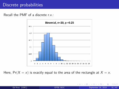
Discrete probabilities
Recall the PMF of a discrete r.v.:
Here, PrpX “ xq is exactly equal to the area of the rectangle at X “ x .
Ed Kroc (UBC) EPSE 581C September 16, 2019 31 / 47

Continuous probabilities
Here, PrpX “ xq “şxx f ptq dt “ 0; i.e. there is no area under the
graph at a single point.
Moreover, notice that for this particular PDF, f p0q ą 1. So the PDFf pxq does not encode probabilities in its values (unlike a PMF).
Ed Kroc (UBC) EPSE 581C September 16, 2019 32 / 47

Continuous probabilities
So for a continuous r.v. X :
PrpX “ xq “ 0 always
Prpa ď X ď bq “şba f pxq dx
Thus, it is the integral of the PDF that encodes probabilities forcontinuous r.v.s, not simply the PDF.
Also, we must always consider a range of possible values for X , otherwisewe will always be considering events that cannot happen.
Note, because the area under the graph at a single point is always zero:
Prpa ď X ď bq “ Prpa ă X ď bq “ Prpa ď X ă bq “ Prpa ă X ă bq
Ed Kroc (UBC) EPSE 581C September 16, 2019 33 / 47

Towards Bayes’ Theorem
Remember: we are trying to get to a point where we can make senseof a continuous version of Bayes’ Theorem.
We have PDFs for continuous random variables.
We know how to calculate probabilities for these random variables viaintegration.
Finally, we need to understand how conditional probability works forcontinuous random variables. To do this, we need to talk about jointdistributions of more than one random variable at the same time.
Ed Kroc (UBC) EPSE 581C September 16, 2019 34 / 47

Joint discrete random variables
Let X and Y be two discrete random variables.
The joint probability mass function of X and Y is:
ppx , yq “ PrpX “ x ,Y “ yq.
Note, we require 0 ď ppx , yq ď 1 for all x , y , andř
x
ř
y ppx , yq “ 1.
Example: X denotes flipping a fair coin and Y denotes rolling a fair6-sided die. Then
PrpX “ H, Y P t1, 2uq “ PrpX “ H, Y “ 1q ` PrpX “ H, Y “ 2q
“1
2¨
1
6`
1
2¨
1
6
“1
6
Ed Kroc (UBC) EPSE 581C September 16, 2019 35 / 47

Joint discrete random variables
Let X and Y be two discrete random variables.
The marginal probability mass functions of X and Y are:
For X : PrpX “ xq “ÿ
all y
ppx , yq
For Y : PrpY “ yq “ÿ
all x
ppx , yq
Example: X denotes flipping a fair coin and Y denotes rolling a fair6-sided die. Then
PrpX “ Hq “ÿ
all y
ppH, yq
“
6ÿ
i“1
PrpX “ H, Y “ iq
“1
2¨
1
6`
1
2¨
1
6` ¨ ¨ ¨ `
1
2¨
1
6“
1
2Ed Kroc (UBC) EPSE 581C September 16, 2019 36 / 47
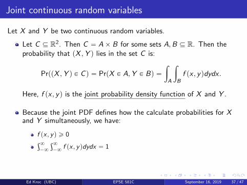
Joint continuous random variables
Let X and Y be two continuous random variables.
Let C Ď R2. Then C “ Aˆ B for some sets A,B Ď R. Then theprobability that pX ,Y q lies in the set C is:
PrppX ,Y q P C q “ PrpX P A,Y P Bq “
ż
A
ż
Bf px , yqdydx .
Here, f px , yq is the joint probability density function of X and Y .
Because the joint PDF defines how the calculate probabilities for Xand Y simultaneously, we have:
f px , yq ě 0ş8
´8
ş8
´8f px , yqdydx “ 1
Ed Kroc (UBC) EPSE 581C September 16, 2019 37 / 47

Joint continuous random variables
If X and Y are both normally distributed, then their joint density f px , yq isgiven by a multivariate bell curve and defines a multivariate normaldistribution:
Ed Kroc (UBC) EPSE 581C September 16, 2019 38 / 47
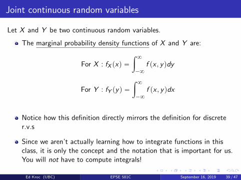
Joint continuous random variables
Let X and Y be two continuous random variables.
The marginal probability density functions of X and Y are:
For X : fX pxq “
ż 8
´8
f px , yqdy
For Y : fY pyq “
ż 8
´8
f px , yqdx
Notice how this definition directly mirrors the definition for discreter.v.s
Since we aren’t actually learning how to integrate functions in thisclass, it is only the concept and the notation that is important for us.You will not have to compute integrals!
Ed Kroc (UBC) EPSE 581C September 16, 2019 39 / 47

Independence of random variables
Two random variables X and Y are said to be independent if and only if:
PrpX “ x ,Y “ yq “ PrpX “ xqPrpY “ yq for discrete X , Y , or,
f px , yq “ fX pxqfY pyq for continuous X , Y .
Example: recall the example of the fair coin and the fair die. Thoserandom phenomena (discrete random variables) were independent, e.g.:
PrpX “ H, Y P t1, 2uq “ PrpX “ H, Y “ 1q ` PrpX “ H, Y “ 2q
“1
2¨
1
6`
1
2¨
1
6
“1
6“ PrpX “ HqPrpY P t1, 2uq
“1
2¨
2
6“
1
6
Ed Kroc (UBC) EPSE 581C September 16, 2019 40 / 47

Conditional distributions
Let X and Y be discrete random variables.
The conditional probability mass function of X given Y “ y , forPrpY “ yq ą 0, is:
PrpX “ x | Y “ yq “PrpX “ x ,Y “ yq
PrpY “ yq
Notice that this is just the ordinary definition of conditionalprobability from last time!
Note: if X and Y are independent, then
PrpX “ x | Y “ yq “PrpX “ xqPrpY “ yq
PrpY “ yq“ PrpX “ xq
Ed Kroc (UBC) EPSE 581C September 16, 2019 41 / 47

Conditional distributions
Example: let Y denote the outcome of a toss of a fair 6-sided die, and letX denote the number of heads that comes up after tossing a fair coin Ymany times.
Then the conditional random variable X | Y „ BinpY , 0.5q.
For example,
PrpX “ 1 | Y “ 2q “PrpX “ 1,Y “ 2q
PrpY “ 2q
“PrpHT , Y “ 2q ` PrpTH, Y “ 2q
PrpY “ 2q
“PrpHT qPrpY “ 2q ` PrpTHqPrpY “ 2q
PrpY “ 2q
“
14 ¨
16 `
14 ¨
16
16
“1
2
Ed Kroc (UBC) EPSE 581C September 16, 2019 42 / 47

Conditional distributions
Let X and Y be continuous random variables.
The conditional probability density function of X given Y “ y , forfY pyq ą 0, is fX |Y px |yq, also denoted fX |Y“y pxq:
fX |Y“y pxq “f px , yq
fY pyq
Notice that this is equivalent to
f px , yq “ fX |Y“y pxq ¨ fY pyq
If X and Y are independent, then
fX |Y“y pxq “fX pxqfY pyq
fY pyq“ fX pxq
Ed Kroc (UBC) EPSE 581C September 16, 2019 43 / 47

Bayes’ Theorem
Finally! We are now prepared to state and prove Bayes’ Theorem forcontinuous random variables.
Bayes’ Theorem
Let X be a continuous random variable; i.e. can take on any real number.Let Y be any random variable (discrete or continuous). Then thedistribution of X given Y is determined by the conditional PDF:
fX |Y“y px | Y “ yq “fY |X“xpy | X “ xqfX pxq
ş8
´8fY |X“tpy | X “ tqfX ptq dt
or, more simply:
f px | yq “f py | xqf pxq
ş8
´8f py | tqf ptq dt
Ed Kroc (UBC) EPSE 581C September 16, 2019 44 / 47

Bayes’ Theorem
Proof of Bayes:
f px | yq “f px , yq
f pyq(defn. cond. PDF)
“f py | xqf pxq
f pyq(defn. cond. PDF)
“f py | xqf pxq
ş8
´8f pt, yq dt
(defn. marg. PDF)
“f py | xqf pxq
ş8
´8f py | tqf ptq dt
(defn. cond. PDF)
Recall: a PDF totally characterizes the probability distribution of arandom variable/phenomenon.
Thus: we can now “partition” a continuum of events and flip the order ofconditioning!
Ed Kroc (UBC) EPSE 581C September 16, 2019 45 / 47

Bayes’ theorem to Bayesian methodology
Critical terminology:
Likelihood
Prior probability
Posterior probability
Normalizing factor
Ed Kroc (UBC) EPSE 581C September 16, 2019 46 / 47

Bayes’ theorem to Bayesian methodology
The posterior probability reflects the updated belief in ahypothesis/event, given the data and the initial prior.
The likelihood is easy to calculate (determined by the model and thedata).
The prior is not determined by the data; the researcher must set itsvalue using prior information.
The normalizing factor only acts as a scaling factor (so that theconditional PDF integrates to 1); it depends on the data, the model,and the prior, but it does not depend on the particularhypothesis/event of interest.
All of Bayesian inference is based on properties of the posteriordistribution/density.
Ed Kroc (UBC) EPSE 581C September 16, 2019 47 / 47