www.electricitypolicy.org.uk

EPR

G W

OR

KIN

G P

APE

R

NO

N-T

EC

HN

ICA

L S

UM

MA

RY

The Effect of Energy Prices on Operation and Investment in OECD Countries: Evidence from the Vintage Capital Model

EPRG Working Paper 0922 Cambridge Working Paper in Economics 0933

Jevgenijs Steinbuks, Andreia Meshreky, and Karsten Neuhoff Empirical analysis of the effect of energy prices on energy use has been so far limited by the ability of econometric models to reflect the adaptation of the capital stock to energy price changes. This paper attempts to address this limitation in by modelling the effect of energy prices on energy use. Our econometric model explicitly incorporates the capital stock, and separately accounts for operational and investment choices in different sectors. Specifically, we expand the traditional estimation of energy, materials, and labour responses to input price changes by including vintages for the capital stock. Each vintage of the capital stock has its own energy efficiency, which is a function of input prices at the time of investment, and the exogenous technological change. In our vintage capital model, a rational cost-minimizing firm chooses both the optimal input quantities and the efficiency of new capital stock. The model therefore separately accounts separately for the flexibility of substitution between input factors to for production (labour, energy and materials), and the potential for more efficient use of these inputs by choosing more efficient technologies at the time of investment. In doing so, our model allows for adaptation of the capital stock to energy price shocks. Our analysis is based on a new panel dataset, which covers 23 OECD countries and four sectors (agriculture, commerce, manufacturing, and transport) between 1990 and 2005. Compared to earlier studies, our analysis relies on more accurate energy prices in different sectors and countries based on the end-use fuel prices and sector-specific energy mix. As a result, this study is among the few to analyze the effect of energy prices from a cross-country, cross-sector perspective.

www.electricitypolicy.org.uk

EPR

G W

OR

KIN

G P

APE

R

NO

N-T

EC

HN

ICA

L S

UM

MA

RY

We estimate the vintage capital model using a translog cost function approach, allowing for non-linearity in factor prices. This introduces additional complexity for the estimation of the relevant parameters of the model, and provides a better explanation of energy demand at the sector level. The assumption of constant efficiency of capital stock is rejected for all sectors. The results for all sectors indicate that rising energy prices result in substantial decline in the long-run energy use, and affect both the operation (input substitution) and the investment (energy efficiency of capital stock) components of energy demand. However, only the estimates for the manufacturing sector can be reconciled with the economic intuition. The vintage capital model predicts that between 1990 and 2005 the energy efficiency of capital stock in the U.S. manufacturing sector has improved by about 24 percent. Interpretation of the results for other sectors is plagued by exogenous structural shifts within and across sectors, regulatory distortions, and measurement error. More robust results would require longer time series and less aggregation across sectors, covering more variation in energy prices.

Contact js782@cam.ac.uk Publication August 2009 Financial Support UK Engineering and Physical Science Research

Council, Grant Supergen Flexnet

www.electricitypolicy.org.uk

EP

RG

WO

RK

ING

PA

PE

R

Abstract

The Effect of Energy Prices on Operation and Investment in OECD Countries: Evidence from the Vintage Capital Model

EPRG Working Paper 0922

Cambridge Working Paper in Economics 0933

Jevgenijs Steinbuks, Andreia Meshreky, and Karsten Neuhoff

This paper analyzes the effect of energy prices on energy efficiency, separately accounting for operational and investment choices in different sectors. For this purpose, capital stock is characterised by vintages with different intensities of energy use, calculated as a function of exogenously-evolving technology availability and energy prices. Our model separately accounts for substitution between inputs to for production (labour, energy and materials), and the potential for more efficient use of these inputs by choosing more efficient technologies at the time of investment. The model is estimated for 23 OECD countries across four sectors, and their respective prices for final energy consumption over the period 1990-2005. Vintage representation of capital stock significantly improves the explanatory value of the model at the sector level. Our results imply that rising energy costs result in substantial decline in energy use in the long-run.

Keywords energy efficiency, energy prices, investment, vintage capital model

JEL Classification D24, E22, Q41, Q43

Contact js782@cam.ac.uk Publication August 2009 Financial Support UK Engineering and Physical Science Research Council,

Grant Supergen Flexnet

The E¤ect of Energy Prices on Operation andInvestment in OECD Countries: Evidencefrom the Vintage Capital Model�

Jevgenijs Steinbuksy, Andreia Meshreky, and Karsten Neuho¤Faculty of Economics, University of Cambridge

Abstract

This paper analyzes the e¤ect of energy prices on energy e¢ ciency, separately ac-counting for operational and investment choices in di¤erent sectors. For this purpose,capital stock is characterised by vintages with di¤erent intensities of energy use, calcu-lated as a function of exogenously-evolving technology availability and energy prices.Our model separately accounts for substitution between inputs for production (labour,energy and materials), and the potential for more e¢ cient use of these inputs by choos-ing more e¢ cient technologies at the time of investment.The model is estimated for 23 OECD countries across four sectors, and their re-

spective prices for �nal energy consumption over the period 1990-2005. Vintage repre-sentation of capital stock signi�cantly improves the explanatory value of the model atthe sector level. Our results imply that rising energy costs result in substantial declinein energy use in the long-run.Keywords: energy e¢ ciency, energy prices, investment, vintage capital modelJEL classi�cation: D24, E22, Q41, Q43

1 Introduction

Empirical analysis of the e¤ect of energy prices on energy use has been so far limited by the

ability of econometric models to re�ect the adaptation of the capital stock to energy price

changes. Gri¢ n and Schulman (2005, p.5) describe the problem as follows: "In a properly

speci�ed econometric demand model, the stocks of energy-using equipment would be mod-

eled with of a number of investment and depreciation equations for each type of energy using�The authors are especially grateful to David Newbery for his contribution to this paper. We also thank

Terry Barker, Gerald Granderson, Michael Grubb, Fred Joutz, M. Hashem Pesaran, Thomas Weber, AnthonyYezer, and seminar participants at Central European University, Miami University, University of Cambridge,the EPRG 2008 Winter Research Simposium at the University of Cambridge, and Supergen FlexNet 2009General Assembly at the University of Manchester for helpful comments and suggestions. All remainingerrors are ours. Financial support from UK Engineering and Physical Science Research Council, GrantSupergen Flexnet is greatly acknowledged.

yCorresponding author. E-mail: js782@cam.ac.uk

1

capital. Energy consumption would then depend on the utilization and e¢ ciency character-

istics of the stock of equipment. Such an elaborate model could then be simulated to describe

the adaptation of the capital stock to energy price shocks. But given the absence of capital

stock data needed to re�ect the adjustment of the capital stock of energy using equipment,

econometricians estimate reduced form single demand equations featuring a distributed lag

on price to capture the adaptation of the capital stock."

This paper attempts to address this limitation in modelling the e¤ect of energy prices on

energy use. Our econometric model explicitly incorporates the capital stock, and separately

accounts for operational and investment choices in di¤erent sectors. Speci�cally, we expand

the traditional estimation of energy, materials, and labour responses to input price changes

by including vintages for the capital stock. Each vintage of the capital stock has its own

energy e¢ ciency, which is a function of input prices at the time of investment, and exogenous

technological change. In our vintage capital model, a rational cost-minimizing �rm chooses

both the optimal input quantities and the e¢ ciency of new capital stock. The model therefore

accounts separately for the �exibility of substitution between input factors to production

(labour, energy and materials), and the potential for more e¢ cient use of these inputs by

choosing more e¢ cient technologies at the time of investment. In doing so, our model allows

for adaptation of the capital stock to energy price shocks.1

Our analysis is based on a new panel dataset, which covers 23 OECD countries and

four sectors (agriculture, commerce, manufacturing, and transport) between 1990 and 2005.

Compared to earlier studies, our analysis relies on more accurate energy prices in di¤erent

sectors and countries based on the end-use fuel prices and sector-speci�c energy mix. As a

result, this study is among the few to analyze the e¤ect of energy prices from a cross-country,

cross-sector perspective.2

We estimate the vintage capital model using a translog cost function approach suggested

by Berndt and Wood (1975). However, our cost-share equations are non-linear in factor

prices because of the composite e¤ect of input substitution and changes in the e¢ ciency

of capital stock. This introduces additional complexity for the estimation of the relevant

parameters of the model, and provides a better explanation of energy demand at the sector

1An alternative econometric approach, which allows for adaptation of capital stock to energy prices isthe quasi-�xed input demand model (Berndt, Morrison, and Watkins 1981; Pindyck and Rotemberg 1983;Popp 2001; and Sue Wing 2008). This approach is based on entirely di¤erent assumptions about the natureof the adaptation of the capital stock, and should be treated complementary to our model. For comparisonof these approaches (and defense of the vintage capital approach), see Atkeson and Kehoe (1999).

2A large number of studies have considered the e¤ect of energy prices from a cross-country within-sector (typically, manufacturing and residential sectors) perspective. The only econometric study known toauthors based on cross-country time-series data disaggregated by sector activity and fuel type, which usestheoretically appropriate measures of income and price is Pesaran, Smith, and Akiyama (1998)

2

level. The assumption of constant e¢ ciency of capital stock is rejected for all sectors.

The results for all sectors indicate that rising energy prices result in substantial decline

in the long-run energy use, and a¤ect both the operation (input substitution) and the invest-

ment (energy e¢ ciency of capital stock) components of energy demand. However, only the

estimates for the manufacturing sector can be reconciled with the economic intuition. The

vintage capital model predicts that between 1990 and 2005 the energy e¢ ciency of capital

stock in the U.S. manufacturing sector has improved by about 24 percent. Interpretation

of the results for other sectors is plagued by exogenous structural shifts within and across

sectors, regulatory distortions, and measurement error. More robust results would require

longer time series and less aggregation across sectors, covering more variation in energy

prices.

The rest of this paper is structured as follows. The �rst section reviews existing liter-

ature on the e¤ect of energy prices on energy e¢ ciency. The second section outlines the

vintage capital model and resulting stochastic speci�cation. The third section describes the

dataset. The fourth section presents the main �ndings of the research. The �fth section

presents the results of policy simulations. The �nal section concludes, and suggests policy

recommendations.

2 Literature Review

The e¤ect of energy prices on energy use is a complex problem, which is still not well

quanti�ed. The economic literature identi�es several channels through which prices in�uence

energy demand in the short, medium and long-run. In the short-run, the main channel is

input substitution, which captures the e¤ect of relative energy prices on the optimal choice

of inputs to production. An increase in real energy prices lowers the demand for energy

services and their complements (e.g. capital), and raises the demand for substitutes to

energy services (e.g. labor). This channel is well studied both theoretically and empirically

based on capital-labor-energy-materials (KLEM) input demand model (Berndt and Wood

1975, Gri¢ n and Gregory 1976, and Pindyck 1979).3

In the medium run, two important channels are the change in the industry structure of

the economy, and improvements in energy e¢ ciency of the capital stock. The change in the

industry structure of the economy takes place because an increase in the real price of energy

services raises the price of intermediate and �nal goods throughout the economy, leading to

series of price and quantity adjustments, with energy-e¢ cient goods and sectors likely to gain

at the expense of energy-intensive ones (Sorrell and Dimitropoulos 2008, p.637). Though

3For a summary of subsequent studies on this topic, see e.g. Barker, Ekins, and Johnstone (1995), andKilian (2008)

3

large number of studies in energy economics attempted to assess the scope of this channel4,

their �ndings are still di¢ cult to reconcile. Two recent empirical contributions are studies

by Metcalf (2008) and Sue Wing (2008). Both studies decompose changes in the aggregate

energy intensity into shifts in the structure of sectoral composition and adjustments in the

e¢ ciency of energy use. Metcalf (2008) adapts an index number based theoretical approach,

and �nds that "roughly three-quarters of the improvements in U.S. energy intensity since

1970 results from e¢ ciency improvements" (Metcalf 2008, p.1). Sue Wing�s (2008) structural

model attributes most of the changes in the U.S. energy intensity to adjustments of quasi-

�xed inputs and disembodied autonomous technological progress. The study concludes that

"price-induced substitution of variable inputs generated transitory energy savings, while

innovation induced by energy prices had only a minor impact." (Sue Wing 2008, p.21).

In the medium-run, �rms also respond to an increase in real energy prices by chang-

ing their investment decisions and improving the energy e¢ ciency of their capital stock

(achieving smaller energy input requirements per unit of capital). For example, �rms in

the commercial sector may insulate their o¢ ce buildings, and �rms in transport sector may

adopt hybrid vehicles to achieve better mileage per gallon. Atkeson and Kehoe (1999) estab-

lish a theoretical foundation of this channel by analyzing energy e¢ ciency in the context of

a putty-clay model. In their model, each vintage of the capital stock has its own energy e¢ -

ciency. In the short-run, capital and energy inputs are the complements, and energy demand

elasticity is small. In the long-run, in response to permanent energy price changes, agents

invest in capital goods with di¤erent energy e¢ ciency. As a result, energy use becomes more

responsive to energy prices.5 Notwithstanding sound theoretical underpinnings, there is little

empirical work on the e¤ect of energy prices on the energy e¢ ciency of capital stock.6 This

paper attempts to address this shortcoming in the empirical literature on energy e¢ ciency.

In the long-run, a signi�cant channel is technological change, both exogenous (e.g. re-

sulting from autonomous scienti�c advance), and energy-price induced. This channel was

studied empirically by Newell, Ja¤e, and Stavins (1999), Popp (2002), Gri¢ n and Schul-

man (2005), Frondel and Schmidt (2006), and Linn (2008). All of these research works use

di¤erent methodologies and reach di¤erent conclusions. Newell, Ja¤e, and Stavins (1999)

develop a product-characteristics model of energy-saving consumer durables, and �nd that

the energy price has little e¤ect on the rate of overall innovation, but it does a¤ect the

direction of innovation for some products. Popp (2002) estimates a structural model, using

4For a survey of these studies, see Ang and Zhang (2000).5Diaz, Puch and Guillo (2004) relax some assumptions of Akeson and Kehoe (1999), and reach similar

conclusions.6A notable exception is a study by Newell, Ja¤e, and Stavins (1999), but their analysis focuses only on

three particular products (room air conditioners, central air conditioners, and gas water heaters).

4

U.S. patent data as an instrument for scienti�c knowledge, and �nds that both energy prices

and the quantity of existing knowledge have very signi�cant positive e¤ects on innovation in

the energy sector. Frondel and Schmidt (2006) compare energy-price elasticities of capital

before and after the oil crisis of the early 1970s. The results of their counterfactual analysis

indicate a substantial technological change, but its magnitude is unknown because of the

change in economic circumstances. Gri¢ n and Schulman (2005) argue that energy-saving

technical change explains asymmetric price responses in econometric energy demand mod-

els.7 Linn (2008) uses the U.S. plant-level data to compare the energy intensity of entrants

and incumbents. The results of Linn�s (2008) empirical analysis show that energy prices and

technology adoption have a small e¤ect on energy intensity.

3 Vintage Capital Model of Energy Demand

We introduce vintage capital model that separately accounts for investment and operational

(production) decisions. We start with the �rms�investment. Firms add new capital stock

based on speci�c production technology. For each capital vintage �rms choose the optimal

level of factor e¢ ciency of production technology given their expectations of future input

costs.

We then consider production decisions, where �rms minimise realized input costs to

produce the desired output level given the level of input e¢ ciency of installed production

technology. The resulting equations are subsequently used to form stochastic speci�cations

and estimate the input price elasticities of factor substitution and capital stock e¢ ciency.

3.1 Investment Choice of Input E¢ ciency

We assume that economic behaviour in OECD country i at time t can be represented by

that of a rational cost-minimizing �rm assumed to operate in perfectly competitive product

and factor markets. The �rm is fully �exible in its choice of labor (xli;t), energy (xei;t), and

materials (xmi;t) inputs. The capital stock (xki;t) has a vintage representation, and each vintage

has its own technological e¢ ciency with respect to each input to the production function.

The investment in factor e¢ ciency of a capital vintage is sunk. New capacity with a di¤erent

production technology can be added, but all old vintages must depreciate before adjustment

is complete.8

We assume that the e¢ ciency of a capital vintage in period q with respect to input j is

represented by an index ji;q: While �rms make technology choices in period q; there is a lag

7Also see Gately and Huntington (2002), and Adeyemi and Hunt (2007).8Our model is thus based on the assumption of putty-clay capital production technologies (for discussion

of this assumption see Atkeson and Kehoe 1999). Other studies that adopt putty-clay models of energy useare Hawkins (1978), Abel (1983), Struckmeyer (1986), Struckmeyer (1987), and Wei (2003).

5

between the �rm�s investment decision and plant commissioning. The technology is installed

and becomes fully functional in period q + 1: Firm�s production decisions in period q are

thus made based on production technology set up in period q � 1.The quantity of input j in period q; xji;q; and the index of input e¢ ciency of capital

vintage, ji;q�1, determine the input service to production function, exji;q:exji;q = xji;q

ji;q�1; ji;q > 0 . (1)

Similarly, the relationship between the price of input in period q; wji;q and the price of

service ewji;q is given by ewji;q = wji;q ji;q�1: (2)

The input e¢ ciency that �rms choose for energy, labour and materials is a function of

the input prices and the exogenous technological change:

ji;q = (1� �)q wji;qwj

!��j; (3)

where wj =

nXi=1

TXt=1

wji;t

nTis the average price of input j across countries and all time

periods9, and � is the rate of exogenous Hicks-neutral technological change10. In appendix

1 we show this is the pro�t maximising (cost minimising choice) of a �rm that faces a

technology cost function.

Then, for all observed capital vintages we derive the index of input e¢ ciency of capital

stock e ji;t as a sum of historic vintage e¢ ciencies weighted by each vintage�s q contribution

to capital stock xkt :

e ji;t = tXq=1

(1� �)q wji;qwj

!��jIi;q (1� �)t�q

xki;t; (4)

9We have chosen the OECD average input price across countries and all time periods to re�ect thee¤ects of globalization and industry migration. For sectors that are less globally integrated (e.g. agriculture,

transport) we also considered the input price based on the country average across time: wji =TXt=1

wji;t=T:

Estimation results are available from authors upon request.10While there is an evidence that technological change responds endogenously to energy prices (see e.g.

Popp 2002), endogenizing technological change is precluded by the numerical complexity of the model. Giventhis, our results should be interpreted as the lowest boundary of the e¤ect of energy prices on energy e¢ ciencyof the capital stock.

6

where Ii;q is the vintage investment in period q, and � is the rate of economic depreciation

of capital stock.

Because we do not know the values of the index of input e¢ ciency of capital stock for

vintages outside observation sample, we have to assume that they are the same as in the �rst

period of observation sample. Under this assumption the index of input e¢ ciency of capital

stock becomes

ji;t = (1� �)t xk0

wji;0wj

!��j+

tXq=1

(1� �)q wji;qwj

!��jIi;q (1� �)t�q

xki;t; (5)

where the �rst term on the right hand side is the value of the index of input e¢ ciency of

capital stock in the �rst period of observation sample.11

3.2 Production Choice of Input Factors

We assume that �rm minimises the costs of its inputs to deliver the output Y :

minX

j=k;l;e;m

wji;txji;t s:t: f(exki;t; exli;t; exei;t; exmi;t) = Yi;t; (6)

where f (�) is continuous, twice di¤erentiable production function relating the �ow of

gross output Yi;t to the services of four inputs - capital�exk�, labor �exl�, energy (exe), and all

other intermediate materials (exm).Let ex�i;t(Yi;t; ewki;t; ewli;t; ewei;t; ewmi;t) be the set of optimal input services, andC(Yi;t; ewki;t; ewli;t; ewei;t; ewmi;t)

be the expenditure function which corresponds to the production function. Following the

economic literature on input demand starting from Christensen, Jorgenson, and Lau (1973)

and Berndt and Wood (1975), we assume that the expenditure function can be approximated

by the translog model:

logCi;t = �0 + �Y log Yi;t +Xj

�ij log ewji;t + 12�Y Y (log Yi;t)2+1

2

Xj

Xk

�ijk log ewji;t log ewji;t +Xj

�Y j log Yi;t log ewji;t + �t+ "jit: (7)

where "jit is the error term. Di¤erentiating (7) with respect to the logarithm of the

prices of e¢ cient inputs, and applying Sheppard�s lemma yields four factor input cost share

11We attempted to estimate the joint e¢ ciency of all unobserved capital stock vintages as a free parameter,but were unable to do so because of limited variation in data.

7

equations

Sji;t = �ij + �Y j log Yi;t +Xj

�ij log ewji;t + "jit; (8)

where Sji;t =@C

@ ewji;t �ewji;tC=

ewji;tex�i;tC

=wji;tx

�i;t

Cis the share of each input j in �rm�s total cost.

3.3 Estimation of Vintage Capital Model

Combining equations (2), (5), and (8) yields a system of four equations to be estimated:

Sji;t = �ij + �Y j log Yi;t+ (9)

Xj

�ij log

0@wji;t24 (1� �)t�1 +

t�1Xq=1

wji;lwj

!��j(1� �)q �i;q

351A+ "jit;

where �ij are country-speci�c �xed e¤ects, which capture the di¤erences in country-

speci�c capital stock outside observation sample, �i;q is the last term in equation (4), and

= xk0

�wji;0wj

���j:12 Following Gri¢ n and Gregory (1976, p. 849) we treat input prices

as purely exogenous, because the small sample bias from a set of constructed instrumental

variables is not necessarily smaller than that obtained from actual prices.

The system of equations (9) is a conditionally linear seemingly unrelated regression13,

which is e¢ ciently estimated by full information maximum likelihood (FIML). Because the

share equations in the model (9) add to one, only 3 share equations are estimated.

The values of parameters � and �j are estimated to maximize the value of the model�s

goodness-of-�t criterion, and are obtained by the grid search. To minimize the computational

burden of a multidimensional grid search, based on earlier empirical �ndings (e.g. Jorgenson

and Fraumeni 1981; Ra¤ and Summers 1987; Baltagi and Gri¢ n 1988; Newell, Ja¤e, and

Stavins 1999; Li, Von Haefen, and Timmins 2008; and Sue Wing 2008) we restrict the

exogenous technological change � to lie between -0.01 and 0.04 and the elasticity of input

e¢ ciency of capital stock with respect to input price changes �j - between 0 and 1.5.

While the system (9) forms our basic empirical model we also estimate a restricted model,

assuming that input e¢ ciency of capital stock does not change, so ji;t is set to 1 (or both

12Our econometric approach described by equation (9) is similar to Haas and Schipper (1998), who ad-vocate calculating an index of energy e¢ ciency, and using it directly in econometric speci�cation for energydemand. The index of Haas and Schipper (1998) though is obtained through factor decomposition, and isthus purely exogenous.13e.g. we still need to obtain the values of � and �j before estimating the model (9) as a linear problem.

8

� and �j are set to zero). Under this restriction the model becomes a conventional translog

model of input demand of Berndt and Wood (1975) and Gri¢ n and Gregory (1976). We

then use the likelihood-ratio test to evaluate the signi�cance of input e¢ ciencies of capital

stock in the models of energy demand.

To quantify factor response to current price changes holding all previous prices constant,

we compute own-price and cross-price elasticities of substitution.14 These elasticities are

given by

�jj =@ lnxji;t

@ lnwji;t=�jj +

�Sji;t�2 � Sji;t

Sji;t; j = k; l; e;m: (10)

and

�pj =@ lnxji;t@ lnwpi;t

=�pj + Spi;tS

ji;t

Sji;t; p; j = k; l; e;m; p 6= j: (11)

Because analysis is based on the panel data across countries, the estimated elasticities

have a standard interpretation of the long-run equilibrium e¤ects (Gri¢ n and Gregory 1976).

Inclusion of capital vintages does not a¤ect this interpretation of computed elasticities, be-

cause capital stock adjusts fully to equilibrium in the long run.

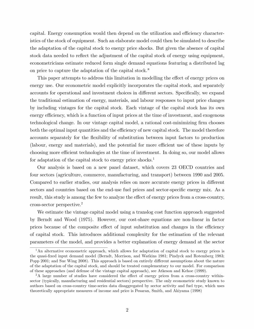
4 Data

Our model is estimated using the panel data of 23 OECD countries separately for four

sectors - agriculture (ISIC sector A), manufacturing (ISIC sector C), commerce (ISIC sector

G), and transportation (ISIC sector H). The main data source for empirical analysis is the

EU KLEMS database. The EU KLEMS database comprises of data on production inputs,

labor and capital input prices15, and output at the industry level for the European Union,

United States, Korea, and Japan. The data is constructed based on the methodology set

by Jorgenson, Gollop, and Fraumeni (1987) and Jorgenson, Ho, and Stiroh (2005).16 The

time coverage for di¤erent series varies signi�cantly across countries and sectors. To ensure

best country coverage we estimate the system of share equations (8) based on an unbalanced

14We have also estimated Allen�s and Morishima�s partial elasticities of substitution. Because these elas-ticities have less straightforward interpretation (Frondel 2004), and can be directly inferred from estimatedcross-price elasticities, their estimates are not reported and available from authors upon request.15Data on the price of capital services were not available for some countries. For these countries following

Andrikopoulos, Brox, and Paraskevopoulos (1989) and Cho, Nam, and Pagán (2004) we computed the capitalinput prices (available from IMF International Financial Statistics Database) as a sum of the nominal interestrate on short-term government papers, and capital depreciation rate.16For more details, see Timmer, O Mahony, and van Ark (2007).

9

panel over the period 1990-2005.17

In our dataset we only have data for capital stock xki;t and do not observe actual invest-

ment. Following large number of empirical studies on investment behaviour (for a survey

see Jorgenson 1971) we assume geometric mortality distribution, (e.g. replacement is pro-

portional to actual capital stock) and time-invariant rate of economic depreciation. Under

these assumptions vintage investment in period q is given by

Ii;q = xki;q � (1� �)xki;q�1: (12)

Based on earlier studies (e.g. Hubbard and Kashyap 1992; Hulten and Wyko¤ 1996;

Nadiri and Prucha 1996; and Jorgenson 1996) we set economic depreciation rates as follows:

economy level - 8%, agriculture - 12%, commerce - 20%, manufacturing - 5%, transport -

20%.

We obtain the end-use energy price data from the International Energy Agency database,

and construct the average sector energy price by weighting energy carriers�prices by the

consumption of each energy carrier in the sector.18

Figure 1 shows average energy prices across di¤erent sectors in OECD countries in 2000.

There are large di¤erences in energy prices across both OECD countries and sectors, because

of variation in energy taxes, types of fuels used in the production process, and local distri-

bution costs. Across sectors, the highest energy prices are in the transport sector, and the

lowest are in the manufacturing sector. Across countries, the highest energy prices are in

European countries (Italy, Ireland, Sweden, and the United Kingdom) and Japan, and the

lowest are in Eastern European economies and the United States. Energy taxes appear to be

the major factor explaining the energy price di¤erences - for example, in 2008 gasoline tax

accounted for nearly 60 percent of �nal energy price in Sweden, Germany and the United

Kingdom, compared to just 13 percent in the United States (International Energy Agency

2008). In contrast, industrial energy prices are similar across OECD countries. This may

re�ect constraints on national energy tax policies in the manufacturing sector, posed by coun-

tries�concerns to maintain their international competitiveness (Brack, Grubb, and Windram

2000).

We construct the price of materials by weighting international commodity prices (from

IMF International Financial Statistics database) by sector consumption of each commod-

17The panel is unbalanced because the data for Czech Republic, Poland, and Slovak Republic were availableas of 1995.18Speci�cally, we consider the following energy products - oil and petrolium products (high- and low-

sulphur fuel oil, light fuel oil, automotive diesel, and gasoline), natural gas, coal, and electricity. Consumptionof each product is measured in British thermal units (BTUs). More details are available in the technicalappendix, available from authors upon request.

10

Figure 1: Average Real Energy Prices across OECD Countries and Sectors in 2005(base year 1995, sorted by manufacturing sector in declining order)

0.0

200.0

400.0

600.0

800.0

1000.0

1200.0

1400.0

1600.0

1800.0

Sweden

Japan

Irelan

dIta

ly

Finland

Austria

Portugal

United K

ingdom

Luxembourg

Denmark

German

yKorea

Spain

Belgium

France

United Stat

es

Australi

a

Netherl

ands

Czech

 Rep

ublic

Greece

Hungary

Slovak R

epublic

Poland

USD

 / to

e

Agriculture Commerce Manufacturing Transport

ity (from UNIDO Industrial production database). The data series for labor, energy, and

material costs, and for the value of output and capital stock are all de�ated to their real

values, using 1995 as a base year, and converted into United States dollars. Full list of

variables, countries and the descriptive statistics for the �nal dataset are shown in Tables

1-3 (Appendix 2).

5 Results of Estimation of Vintage Capital Model

The results for the aggregate OECD economy level and for the four sectors are presented in

Tables 4a-4e (Appendix 2). We present results for both the vintage capital model, and the

standard translog model of energy demand, in which the indices of input e¢ ciency of capital

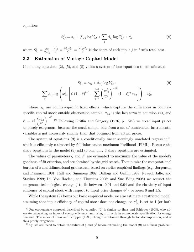
stock are set to 119. Tables 1 and 2 present estimated own-price elasticities of input demand,

cross-price elasticities of energy demand, and own-price elasticities of input e¢ ciency of

capital stock based on the vintage capital model.20 Tables 5a-5e, Appendix 2 demonstrate

variation of estimated elasticities across countries. Estimated cross-price elasticities of other

input demands are presented in Table 6, Appendix 2. Figures 1a-1e, Appendix 3 show the

values of the calculated indices of input e¢ ciency of capital stock.

19This model is refered as a restricted model in Tables 4a-4e of Appendix II.20Estimated elasticities of input demand based on the restricted model are not reported because their size

and magnitude was not substantially di¤erent from the unrestricted model. The results are available fromauthors upon request.

11

Table 1. Estimated Own-Price Elasticities of OECD Input Demand

Sector Sector Share inOECD Gross Output

ηLL ηKK ηEE ηMM ηLE ηKE ηME

Total Economy 100% ­0.27 ­0.81 ­0.10 ­0.60 ­0.05 ­0.11 0.15Agriculture 2.5% ­0.30 ­0.85 ­1.12 ­0.67 0.01 1.74 0.07Commerce 10.6% 0.07 ­0.63 ­1.51 ­0.44 0.09 ­0.09 0.19Manufacturing 31.1% ­0.39 ­0.89 ­1.30 ­0.57 0.18 ­0.05 0.16Transport 6.2% ­0.10 ­1.02 ­0.85 ­1.13 0.45 0.59 0.28

The vintage capital model provides a better explanation of energy demand at both econ-

omy and sector levels. The likelihood ratio test indicates that the restriction of input e¢ -

ciencies of capital stock equal to 1 is rejected at the 1% level of signi�cance for both the

economy-level and sector-level estimates.

Overall, the estimates of own-price and cross-price elasticities of input demand are con-

sistent with their economic interpretation. Table 1 demonstrates that all but one of the

estimated own-price elasticities for input demands across di¤erent sectors have the expected

signs. The only exception is the commerce sector, where the own-price elasticity of labor

demand does not have the expected sign. This outcome may result from endogeneity of

wages and cost shares in labor-intensive commerce sector.

Estimated elasticities of own-price input demand generally have reasonable magnitudes.

The results from the vintage capital model indicate that long-run energy demand is elastic

in all sectors, except for the transport sector, with highest operational response in the man-

ufacturing and commerce sectors. These estimates are higher compared to previous panel

data studies (0.6-0.9). These di¤erences could re�ect a variety of reasons (e.g. technological

change, energy and capital market liberalization, changed economic circumstances, and mea-

surement error), and their empirical assessment is not possible without proper counterfactual

analysis (Frondel and Schmidt 2006). At the economy-level, the estimated own-price energy

demand elasticities are lower than expected. This may re�ect the e¤ect of the residential

sector, where the medium term response to energy prices is highly inelastic.

Table 1 also shows estimated partial cross-price elasticities of energy demand. As ex-

pected, labor and materials are substitutes for energy at the sector level. At the economy

level, the direct elasticities show that energy inputs are substitutes to materials, and com-

plements to labor. Complementarity between labor and energy inputs at the economy level

is puzzling, and is possibly the outcome of the aggregation bias, discussed earlier in this

section.

The relation between energy and capital inputs varies across sectors. The elasticities

indicate that capital and energy are the substitutes in the agriculture and transport sectors,

comparable with the interpretation that larger capital intensity implies modern and energy

12

e¢ cient equipment. In the manufacturing and commerce sectors the elasticity is negative,

indicating that capital and energy are compliments. This result is similar to previous �ndings

(Thompson and Taylor 1995), and re�ects the di¢ culties in measuring the elasticity of

substitution in a multiple factor world.

Table 2. Own-Price Elasticities of Input E¢ ciency of Capital Stock,

Real Input Price Changes, and the Rate of Exogenous Technological Change

in OECD Countries, 1990-2005

Sector γLChange in Real

Wages, % γEChange in Real

Energy Prices, % γMChange in Real

Materials Prices, % ζ

Total Economy 0.65 ­2.34 0.32 6.05 1.26 ­26.82 0.028Agriculture 0.04 59.72 0.73 34.45 0.03 ­8.71 0.032Commerce 0.01 8.05 0.90 ­17.09 0.095 ­30.27 0.022Manufacturing 0.37 22.33 0.32 16.40 0.001 ­6.29 0.025Transport 0.31 20.82 0.82 8.04 0.57 ­27.44 0.035*

* estimate did not meet the boundary condition

Table 2 illustrates the estimated elasticities of input e¢ ciency of capital stock, corre-

sponding real input price changes and the estimated rate of exogenous technological change

in OECD countries between 1990 and 2005. At the sector level, only the estimates for

the manufacturing sector can be reconciled with economic intuition. Estimated own-price

elasticities of labor and energy e¢ ciency of capital stock in the manufacturing sector have

reasonable magnitudes. The own-price elasticity of materials e¢ ciency of capital stock is

close to zero in the manufacturing sector (and also in the agriculture and the commerce

sectors). Table 3 shows that the real price of materials has fallen in all sectors. This result

suggests that capital stock responds little to falling input prices and supports the hypothesis

of asymmetric demand response to input prices (Borenstein, Cameron, and Gilbert 1997;

Peltzman 2000; Gately and Huntington 2002).21 The parameter � in the manufacturing sec-

tor (and all other sectors) is positive, indicating that autonomous technological change rises

input e¢ ciency of capital stock.

Figure 2 illustrates the e¤ect of energy prices on energy e¢ ciency of capital stock, by

showing estimated rate of improvement in energy e¢ ciency in manufacturing sector across

capital vintages in the United States in 1990-2005. The vintage capital model predicts that

between 1990 and 2005 the energy e¢ ciency of capital stock in the U.S. manufacturing sector

has improved by about 24 percent. Real energy prices did not change much before 2000, and

most improvements in the energy e¢ ciency of capital stock were driven by exogenous energy-

saving technological change. The major price-induced improvement in energy e¢ ciency came

between 2000 and 2005, following a sharp rise in real energy prices.21Because of little time series variation in data, this result should be taken with caution.

13

Figure 2: Real Energy prices and Energy E¢ ciency Improvements in the U.S. ManufacturingSector

0% 0% ­ 5% 5%­10% 10% ­ 15% 15% ­ 24%

Improvement in the Energy Efficiency of Capital Stock

0

1000

2000

3000

4000

5000

6000

7000

8000

1990 1991 1992 1993 1994 1995 1996 1997 1998 1999 2000 2001 2002 2003 2004 2005

Rea

l Val

ue o

f Cap

ital S

tock

(US

D b

illio

ns)

0

50

100

150

200

250

300

350

400

Rea

l Ene

rgy 

Pric

es(U

SD / 

toe,

 Bas

e Ye

ar =

 199

5)

Real Energy Price

Capital Stock Vintages

0% 0% ­ 5% 5%­10% 10% ­ 15% 15% ­ 24%0% 0% ­ 5% 5%­10% 10% ­ 15%0% 0% ­ 5% 5%­10% 10% ­ 15% 15% ­ 24%

Improvement in the Energy Efficiency of Capital Stock

0

1000

2000

3000

4000

5000

6000

7000

8000

1990 1991 1992 1993 1994 1995 1996 1997 1998 1999 2000 2001 2002 2003 2004 2005

Rea

l Val

ue o

f Cap

ital S

tock

(US

D b

illio

ns)

0

50

100

150

200

250

300

350

400

Rea

l Ene

rgy 

Pric

es(U

SD / 

toe,

 Bas

e Ye

ar =

 199

5)

Real Energy Price

Capital Stock Vintages

In other sectors of economic activity, the estimated elasticities of input e¢ ciency of capital

stock are not consistent with the economic theory and available evidence. Speci�cally, in

the agriculture and the commerce sectors, the estimated elasticities of labor e¢ ciency of

capital stock are close to zero, and the estimated elasticities of energy e¢ ciency of capital

stock are 2.5-3 times larger than in the manufacturing sector. In the transport sector, the

parameter for autonomous technological change failed to meet boundary conditions, casting

doubts on the interpretation of estimated parameters. We believe that these results are

the consequence of exogenous structural shifts (especially in the new member states of the

European Union)22, regulatory distortions23, and measurement error24. Further research at

less aggregate level is required to explain these results better.

22Havlik (2004) �nds that productivity catching-up observed in the new member states of the EuropeanUnion resulted overwhelmingly from massive shut-downs of unproductive labor- and energy- intensive �rms,especially in the agriculture sector. The employment shifts among sectors had only a negligible e¤ect onaggregate productivity growth.23 for example, Fulginiti and Perrin (1993) �nds that subsidies distort wage-productivity link in the agricul-

ture sector. Regulatory policies in the agriculture and transport sector may also a¤ect the market structure,thus compromising model assumption that �rms are perfectly competitive cost minimizers.24For problem of measurement error in the empirical studies of the service sectors, see (Gordon 1996).

(Timmer, O Mahony, and van Ark 2007) report a number of unresolved issues in the measurement ofintermediate input prices, value added, and the capital stock in the EU KLEMS database.

14

At the economy level, the estimated own-price elasticities of labor and energy e¢ ciency

of capital stock have reasonable values. The estimated elasticity of materials intensity of

capital stock, however, is considerably higher than at the sector level, and is not consistent

with our expectations. Another puzzling result is that the average real wages have declined

at the economy level, and have increased at the sector level. These �ndings suggest that in

addition to the problems discussed in the previous paragraph, the economy-level estimates

re�ect the e¤ect of omitted sectors, and measurement error of non-linear aggregation across

sectors.

6 Simulated E¤ects of Greenhouse Gas Emissions Tax

The results of the model discussed in the previous section indicate that capital stock is

signi�cant in determining the future energy e¢ ciency of production. These �ndings imply

that energy and climate policies providing incentives for early investment in energy e¢ cient

capital stock may reduce future energy (including fossil fuel) input consumption. To illustrate

the outcome of such policies we use the vintage capital model predictions to evaluate the

e¤ect of a greenhouse emissions tax on energy consumption. Because of the di¢ culties with

interpreting economy-level and most of the sector-level estimates described in preceding

section, our analysis is restricted to the manufacturing sector. Speci�cally, we simulate the

e¤ect of the greenhouse gas (carbon dioxide, CO2) emissions tax implemented in 2005.

We assume that all input prices except for the energy prices and output remain at their

2005 levels (e.g. �Yi;t = �wj=k;l;mi;t = 0; t > 2005). The capital stock stays constant, and

the vintage investment o¤sets capital stock depreciation (e.g. xki;t>2005 = xki;2005; �Ii;l>2005 =

(1� �)xki;2005). Based on the results of the vintage capital model (see Table 3 and Table 5d,

Appendix 2) we assume that the rate of exogenous technological change � = 0:025, the own-

price elasticity of energy e¢ ciency of capital stock �e = 0:32; and the own-price elasticity of

energy demand for the U.K. manufacturing sector �ee = �1:44.Figure 3 illustrates the simulation results. In the baseline scenario, we assume there is

no greenhouse emission tax, and energy price does not change. The change in the energy

input consumption in the baseline scenario is determined by two factors. The �rst factor

is the improvement in the energy e¢ ciency of capital stock due to exogenous technological

change. To quantify this e¤ect we use the assumptions above to compute an index of energy

e¢ ciency of the capital stock for the simulation sample based on equation (5). The second

factor is the change in the share of energy service due to the substitution e¤ect between labor,

energy, and materials services.25 We compute the change in the share of energy service using

25Given the assumptions above, the equation (9) implies that �SEi;t =X

j=k;l;e;m

�ij� log�wji;t

ji;t

�=

15

Figure 3: Simulated E¤ect of $30 Carbon Tax on Energy Consumption in the UK Manufac-turing Sector

the results from regression (9) for the manufacturing sector (see Table 4d, Appendix 2),

and convert this change into energy units (toe). Our calculations show that in the baseline

scenario, these factors account for 18 percent decline in energy input consumption by 2020.

In the counterfactual scenario, we assume there is $30 tax per ton of emitted greenhouse

gas. Using the data for the UK manufacturing sector, we �nd that one ton of the fuel mix

emits 2.5 tons of the CO2 (computation details are available in Table 7, Appendix 2).26

Then, a $30 tax per ton of greenhouse gas corresponds to $75 per toe, or (given that average

real energy price in the UK manufacturing sector was $502 per toe) to 15 percent increase

in energy input price.

The change in the energy input consumption in the counterfactual scenario relative to

the baseline scenario depends on two factors. The �rst factor is price-induced change in

the energy e¢ ciency of the capital stock (or the price-induced investment response). AsXj=k;l;e;m

�ij� log(wji;t) +

Xj=l;e;m

�ij� log ji;t =

Xj=l;e;m

�ij� log ji;t 6= 0:

26The data on fuel mix composition in the UK manufacturing sector is obtained from the InternationalEnergy Agency database. The greenhouse emission coe¢ cients per type of fuel (in million of British ThermalUnits, BTU) are obtained from the US Department of Energy Voluntary Reporting of Greenhouse Gases Pro-gram website (http://www.eia.doe.gov/oiaf/1605/coe¢ cients.html) and converted to tons of oil equivalent(toe, 1 toe � 40 x 106 BTU).

16

in the baseline scenario, we compute the index of energy e¢ ciency of the capital stock for

the simulation sample, now assuming a 15 percent increase in the energy input price. Our

calculations show that the price-induced investment response results in 4 percent less energy

consumption relative to that in baseline scenario by 2020. This analysis, however, excludes

the rebound e¤ect27. To quantify the rebound e¤ect, we predict an increase in the share

of energy service consumption Sji;t due to greenhouse tax induced improvements in energy

e¢ ciency of capital stock (holding other factors constant), and convert these changes in level

terms. The rebound e¤ect is the di¤erence in price-induced energy consumption with and

without adjustments for changes in share of energy service. Our calculations show a long-run

rebound e¤ect of 26 percent, which is consistent with the �ndings from previous studies (see

e.g. Small and Van Dender (2007) and references therein). In the presence of the rebound

e¤ect, energy consumption is 3 percent less than in the baseline scenario by 2020.

The second factor is the long-run change in the energy demand due to input substitution

(or the operational response). Because prices of other inputs are assumed constant, the

decline in the long-run energy demand depends solely on the own-price elasticity of energy

demand. Our calculations show that the operational response to the greenhouse emissions

tax results in 21 percent less energy consumption than energy consumption in the baseline

scenario by 2020.

Bringing all e¤ects together, a 15 percent increase in the energy input price due to

the greenhouse gas tax lowers energy consumption by 24 percent relative to the baseline

scenario. Price-induced e¢ ciency improvements lower long-run energy consumption by 4

percent relative to baseline scenario. However, 26 percent of these price-induced e¢ ciency

improvements (or 1 percent of energy consumption in the baseline scenario) are reverted due

to the rebound e¤ect. The remaining 21 percent decline in long-run energy consumption

relative to the baseline scenario is due to a reduction in the long-run energy demand. These

results indicate that energy and climate policies that increase energy costs result in signi�cant

reduction in the energy use in the long-run.

7 Concluding Remarks

We have expanded the traditional estimation of energy, materials, and labour responses to

input price changes by including vintages for the capital stock. The model allows for both

substitution across production inputs (labour, energy and materials), and more e¢ cient use

of these inputs by choosing more e¢ cient technologies at the time of investment.

27In this context the "rebound e¤ect" is de�ned as a direct increase in demand for an energy service whosesupply had increased as a result of improvements in technical e¢ ciency in the use of energy (Khazzoom1980; Greening, Greene, and Di�glio 2000; Sorrell and Dimitropoulos 2008).

17

In order to test the model, we develop a new dataset for 23 OECD countries, and calculate

average �nal energy prices in di¤erent sectors and countries based on fuel prices and the

energy mix within the sector. At the sector level, the explanatory value of the model with

vintage capital stock is signi�cantly improved, and the assumption of constant e¢ ciency of

capital stock is rejected for all sectors.

The results for all sectors indicate that rising energy prices result in substantial decline

in the long-run energy use, and a¤ect both the operation (input substitution) and the invest-

ment (energy e¢ ciency of capital stock) components of energy demand. However, only the

estimates for the manufacturing sector can be reconciled with the economic intuition. The

vintage capital model predicts that between 1990 and 2005 the energy e¢ ciency of capital

stock in the U.S. manufacturing sector has improved by about 24 percent. Interpretation of

the results for other sectors are plagued by exogenous structural shifts, regulatory distortions,

and measurement error.

In further work it will be interesting to explore the robustness of our results by: (1)

expanding the observation period beyond 1990-2005; (2) bringing the analysis to further

disaggregated level of industry activities; and (3) including non-OECD countries in the data

set.

References

Abel, A. (1983). Energy Price Uncertainty and Optimal Factor Intensity: A Mean-

Variance Analysis. Econometrica 51 (6), 1839�1845.

Adeyemi, O. and L. Hunt (2007). Modelling OECD Industrial Energy Demand: Asymmet-

ric Price Responses and Energy-saving Technical Change. Energy Economics 29 (4),

693�709.

Andrikopoulos, A., J. Brox, and C. Paraskevopoulos (1989). Interfuel and Interfactor

Substitution in Ontario Manufacturing, 1962�1982. Applied Economics 21, 1�15.

Ang, B. and F. Zhang (2000). A Survey of Index Decomposition Analysis in Energy and

Environmental Studies. Energy 25 (12), 1149�1176.

Ashenfelter, O. and D. Card (1982). Time Series Representations of Economic Variables

and Alternative Models of the Labour Market. The Review of Economic Studies 49 (5),

761�781.

Atkeson, A. and P. Kehoe (1999). Models of Energy Use: Putty-Putty versus Putty-Clay.

American Economic Review 89 (4), 1028�1043.

18

Baltagi, B. and J. Gri¢ n (1988). A General Index of Technical Change. The Journal of

Political Economy 96 (1), 20�41.

Barker, T., P. Ekins, and N. Johnstone (1995). Global Warming and Energy Demand.

Routledge, London and New York.

Berndt, E., C. Morrison, and G. Watkins (1981). Dynamic Models of Energy Demand: An

Assessment and Comparison. in Measuring and Modeling Natural Resource Substitu-

tion (ed. E. Berndt and B. Field), MIT Press.

Berndt, E. and D. Wood (1975). Technology, Prices, and the Derived Demand for Energy.

The Review of Economics and Statistics 57 (3), 259�268.

Borenstein, S., A. Cameron, and R. Gilbert (1997). Do Gasoline Prices Respond Asymmet-

rically to Crude Oil Price Changes? Quarterly Journal of Economics 112 (1), 305�339.

Brack, D., M. Grubb, and C. Windram (2000). International Trade and Climate Change

Policies. Earthscan.

Cho, W., K. Nam, and J. Pagán (2004). Economic Growth and Interfactor/Interfuel Sub-

stitution in Korea. Energy Economics 26 (1), 31�50.

Christensen, L., D. Jorgenson, and L. Lau (1973). Transcendental Logarithmic Production

Frontiers. The Review of Economics and Statistics 55 (1), 28�45.

Frondel, M. (2004). Empirical Assessment of Energy-Price Policies: the Case for Cross-

Price Elasticities. Energy Policy 32 (8), 989�1000.

Frondel, M. and C. Schmidt (2006). The Empirical Assessment of Technology Di¤erences:

Comparing the Comparable. The Review of Economics and Statistics 88 (1), 186�192.

Fulginiti, L. and R. Perrin (1993). Prices and Productivity in Agriculture. The Review of

Economics and Statistics 75, 471�482.

Gately, D. and H. Huntington (2002). The Asymmetric E¤ects of Changes in Price and

Income on Energy and Oil Demand. Energy Journal 23 (1), 19�56.

Gordon, R. (1996). Problems in the Measurement and Performance of Service-Sector Pro-

ductivity in the United States. NBER Working Paper 5519.

Greening, L., D. Greene, and C. Di�glio (2000). Energy E¢ ciency and Consumption�the

Rebound E¤ect�a Survey. Energy Policy 28 (6-7), 389�401.

Gri¢ n, J. and P. Gregory (1976). An Intercountry Translog Model of Energy Substitution

Responses. American Economic Review 66 (5), 845�857.

19

Gri¢ n, J. and C. Schulman (2005). Price Asymmetry: A Proxy for Energy Saving Tech-

nical Change? The Energy Journal 26 (2), 1�21.

Haas, R. and L. Schipper (1998). Residential Energy Demand in OECD-countries and the

Role of Irreversible E¢ ciency Improvements. Energy Economics 20 (4), 421�442.

Havlik, P. (2004). Structural Change, Productivity and Employment in the New EU Mem-

ber States. WIIW Research Paper 313.

Hawkins, R. (1978). A Vintage Model of the Demand for Energy and Employment in

Australian Manufacturing Industry. Review of Economic Studies 45 (3), 479�94.

Hubbard, R. and A. Kashyap (1992). Internal Net Worth and the Investment Process: An

Application to US agriculture. Journal of Political Economy 100 (3), 506�534.

Hulten, C. and F. Wyko¤ (1996). Issues in the Measurement of Economic Depreciation

Introductory Remarks. Economic Inquiry 34 (1), 10�23.

International Energy Agency, I. (2008). Energy Prices and Taxes, 4th Quarter 2008.

OECD/IEA, Paris, France.

Jorgenson, D. (1971). Econometric Studies of Investment Behavior: a Survey. Journal of

Economic Literature 9 (4), 1111�1147.

Jorgenson, D. (1996). Empirical Studies of Depreciation. Economic Inquiry 34 (1), 24�42.

Jorgenson, D. and B. Fraumeni (1981). Relative Prices and Technical Change. In.: Berndt,

ER (Ed.). Modeling and Measuring Natural Resource Substitution.

Jorgenson, D., F. Gollop, and B. Fraumeni (1987). Productivity and US Economic Growth.

Cambridge, MA: Harvard University Press.

Jorgenson, D., M. Ho, and K. Stiroh (2005). Information Technology and the American

Growth Resurgence. MIT Press.

Khazzoom, J. (1980). Economic Implications of Mandated E¢ ciency in Standards for

Household Appliances. Energy Journal 1 (4), 21�40.

Kilian, L. (2008). The Economic E¤ects of Energy Price Shocks. Journal of Economic

Literature 46 (4), 871�909.

Li, S., R. Von Haefen, and C. Timmins (2008). How Do Gasoline Prices A¤ect Fleet Fuel

Economy? NBER Working Paper 14450.

Linn, J. (2008). Energy Prices and the Adoption of Energy-saving Technology. The Eco-

nomic Journal 118, 1986�2012.

20

Metcalf, G. (2008). An Empirical Analysis of Energy Intensity and Its Determinants at

the State Level. The Energy Journal 29 (3), 1�26.

Nadiri, M. and I. Prucha (1996). Estimation of the Depreciation Rate of Physical and

R&D Capital in the US Total Manufacturing Sector. Economic Inquiry 34 (1), 43�56.

Newell, R., A. Ja¤e, and R. Stavins (1999). The Induced Innovation Hypothesis and

Energy-Saving Technological Change. Quarterly Journal of Economics 114 (3), 941�

975.

Peltzman, S. (2000). Prices Rise Faster than They Fall. Journal of Political Econ-

omy 108 (3), 466�502.

Pesaran, M., R. Smith, and T. Akiyama (1998). Energy Demand in Asian Developing

Economies. Oxford University Press, USA.

Pindyck, R. (1979). Interfuel Substitution and the Industrial Demand for Energy: An

International Comparison. The Review of Economics and Statistics 61, 169�179.

Pindyck, R. (1999). The Long-run Evolution of Energy Prices. The Energy Journal 20 (2),

1�27.

Pindyck, R. and J. Rotemberg (1983). Dynamic Factor Demands and the E¤ects of Energy

Price Shocks. American Economic Review 73, 1066�1079.

Popp, D. (2001). The E¤ect of New Technology on Energy Consumption. Resource and

Energy Economics 23 (3), 215�240.

Popp, D. (2002). Induced Innovation and Energy Prices. American Economic Re-

view 92 (1), 160�180.

Ra¤, D. and L. Summers (1987). Did Henry Ford Pay E¢ ciency Wages? Journal of Labor

Economics 5 (S4), 57.

Small, K. and K. Van Dender (2007). Fuel E¢ ciency and Motor Vehicle Travel: the

Declining Rebound E¤ect. The Energy Journal 28 (1), 25.

Sorrell, S. and J. Dimitropoulos (2008). The Rebound E¤ect: Microeconomic De�nitions,

Limitations and Extensions. Ecological Economics 65 (3), 636�649.

Struckmeyer, C. (1986). The Impact of Energy Price Shocks on Capital Formation and

Economic Growth in a Putty-Clay Technology. Southern Economic Journal 53 (1),

127�140.

Struckmeyer, C. (1987). The Putty-Clay Perspective on the Capital-Energy Complemen-

tarity Debate. The Review of Economics and Statistics 69 (2), 320�326.

21

Sue Wing, I. (2008). Explaining the Declining Energy Intensity of the US Economy. Re-

source and Energy Economics 30 (1), 21�49.

Thompson, P. and T. Taylor (1995). The Capital-Energy Substitutability Debate: A New

Look. The Review of Economics and Statistics 77 (3), 565�69.

Timmer, M., M. O Mahony, and B. van Ark (2007). EU KLEMS Growth and Productivity

Accounts: An Overview. Working Paper, University of Groningen and University of

Birmingham.

Train, K. (1986). Qualitative Choice Analysis: Theory, Econometrics, and an Application

to Automobile Demand. MIT press.

Wei, C. (2003). Energy, the Stock Market, and the Putty-Clay Investment Model. Amer-

ican Economic Review 93 (1), 311�323.

22

Appendix I - Derivation of Firm�s Investment Choice of CapitalVintage E¢ ciencyThe �rm�s choice of production technology depends on input cost savings from new

technology and the costs of setting up new technology. For simplicity, let us assume that

the index of input e¢ ciency of capital vintage in time q � 1 is equal to one. If in periodq the �rm installs the same technology; based on equation (1) the cost of input service to

production function in period q + 1; F ji;q+1; will be given by

F ji;q+1 = E�wji;q+1exji;q+1� = E

�wji;q+1x

ji;q+1

�; (13)

where E (�) denotes the expectations operator.If in period q the �rm installs more e¢ cient technology with the index of input e¢ ciency

of capital vintage ji;q; based on equation (1) the cost of input service to production function

in period q + 1; F 0ji;q+1; will be given by

F 0ji;q+1 = E�wji;q+1exji;q+1� = 1

ji;qE�wji;q+1x

ji;q+1

�< F ji;q+1: (14)

Based on the standard assumptions of the theory of the �rm, we assume that the cost

of installing technology with the index of input e¢ ciency of capital vintage ji;q can be

represented by a continuos, twice-di¤erentiable, and convex cost function g� ji;q�:

Given the assumptions above, �rm�s input cost savings from installing more e¢ cient

technology in period q + 1 are

�ji;t =

1� 1

ji;q

!E�wji;q+1x

ji;q+1

�� g

� ji;q�: (15)

Applying �rst order conditions to equation (15), setting them to zero and solving resulting

equation yields �rms�optimal index of input e¢ ciency of capital vintage �ji;q :

�ji;q = argmax ji;q

"E�wji;q+1x

ji;q+1

�g0� ji;q� � ji;q�2#: (16)

To obtain a closed-form solution for �ji;q one can use in an empirical speci�cation, we

assume that input quantities are predetermined and constant

xji;q = xji;q+1 = xj; (17)

and that the input prices exhibit a random walk28, so that current input prices are the

28This assumption is consistent with evidence found in empirical studies (Ashenfelter and Card 1982;

23

best predictors of future input costs:

E�wji;q+1

�= wji;q; (18)

and the cost of installing technology with the index of input e¢ ciency of capital vintage

ji;q is given by

g� ji;q�=h

'

� ji;q�'; (19)

where h and ' are positive constants determining the curvature of the cost function.

Using equations (18) and (19) in equation (16) yields the closed form solution for �rm�s

investment choice of input e¢ ciency of capital vintage ji;q :

�ji;q =

wji;qx

ji;q

h

! 1'+1

: (20)

Let h = xjwj; where wj =

nXi=1

TXt=1

wji;t

nTis the average price of input j across countries and

all time periods.

Then equation (20) becomes

�ji;q =

wji;qwj

!��j; (21)

where �j = � 1'+1

=@ ji;q

@wji;q

wji;q

ji;qis the elasticity of input e¢ ciency of capital stock with

respect to input price changes. Equation (21) implies that higher input prices result in a

greater input e¢ ciency of capital stock (and the smaller value of ji;q; meaning that smaller

input quantities are required to produce the same amount of output holding capital stock

constant). This result is consistent with theoretical works showing that �rms respond to

input price changes by choosing more e¢ cient technologies for the production process (see

e.g. Khazzoom 1980; Train 1986).

Pindyck 1999).

24

Appendix II - Tables

Table 1

List of Variables

Variable Desctiption UnitsSL Share of Labor in the Total Cost PercentSK Share of Capital in the Total Cost PercentSE Share of Energy in the Total Cost PercentSM Share of Materials in the Total Cost PercentY Gross Output Real USD millionwL Wage Real USD / hourwK Rate of Return on Capital PercentwE Price of Energy USD / toewM Price of Materials USD / metric ton

Table 2

List of Countries

Country ID Country Data Availability1 Australia 1990­20052 Austria 1990­20053 Belgium 1990­20054 Czech Republic 1995­20055 Denmark 1990­20056 Finland 1990­20057 France 1990­20058 Germany 1990­20059 Greece 1990­200510 Hungary 1991­200511 Ireland 1990­200512 Italy 1990­200513 Japan 1990­200514 Korea 1990­200515 Luxembourg 1990­200516 Netherlands 1990­200517 Poland 1995­200518 Portugal 1990­200519 Slovak Republic 1995­200520 Spain 1990­200521 Sweden 1990­200522 United Kingdom 1990­200523 United States 1990­2005

25

Table 3a

Descriptive Statistics, Economy Level (1995)

Country SL SK SE SM Y wL wK wE wM

Australia 0.40 0.24 0.05 0.31 752265 17.2 0.13 488.9 842.1Austria 0.44 0.22 0.04 0.30 397074 26.4 0.11 774.6 1153.1Belgium 0.39 0.21 0.05 0.35 566882 36.1 0.11 625.2 1221.2Czech Republic 0.27 0.21 0.07 0.45 131888 3.3 0.09 371.0 800.4Denmark 0.43 0.23 0.04 0.30 297992 29.0 0.12 719.5 1048.7Finland 0.39 0.19 0.06 0.36 237054 26.0 0.13 675.0 1064.0France 0.44 0.22 0.05 0.29 2702751 29.6 0.12 685.4 1219.7Germany 0.46 0.22 0.05 0.28 4284886 31.4 0.10 729.3 1394.4Greece 0.36 0.30 0.06 0.28 183821 13.9 0.21 642.1 1182.9Hungary 0.34 0.21 0.08 0.37 89768 4.1 0.33 364.8 1398.9Ireland 0.35 0.21 0.05 0.40 138429 19.5 0.12 644.2 1709.9Italy 0.39 0.19 0.06 0.36 2103766 25.6 0.18 780.6 1296.2Japan 0.39 0.26 0.04 0.31 9713929 31.9 0.07 1030.4 1162.5Korea 0.39 0.13 0.05 0.43 1081649 10.8 0.16 411.4 1077.9Luxembourg 0.39 0.30 0.07 0.24 38167 33.3 0.11 596.2 1709.5Netherlands 0.41 0.20 0.05 0.34 787729 29.9 0.11 574.7 1281.0Poland 0.41 0.15 0.06 0.37 264868 5.2 0.27 267.5 1085.3Portugal 0.36 0.19 0.05 0.39 213649 9.4 0.16 671.0 1134.9Slovak Republic 0.24 0.25 0.07 0.44 45299 2.4 0.14 265.5 899.9Spain 0.37 0.22 0.05 0.36 1138641 18.5 0.13 636.1 1226.9Sweden 0.40 0.22 0.05 0.33 455543 22.9 0.15 665.7 947.8United Kingdom 0.43 0.18 0.06 0.33 2100778 19.1 0.13 600.2 1036.1United States 0.46 0.26 0.05 0.23 12900000 20.2 0.11 355.9 1313.4

Table 3b

Descriptive Statistics, Agriculture (1995)

Country SL SK SE SM Y wL wK wE wM

Australia 0.31 0.22 0.08 0.39 27333 9.2 0.13 606.7 1394.4Austria 0.56 0.05 0.08 0.30 10963 10.0 0.11 797.0 1661.8Belgium 0.28 0.14 0.17 0.41 9768 21.3 0.11 523.1 1360.9Czech Republic 0.24 0.14 0.24 0.37 5723 2.1 0.09 590.6 1379.9Denmark 0.25 0.25 0.10 0.40 11779 15.2 0.12 425.4 1279.2Finland 0.52 0.04 0.11 0.33 9185 11.2 0.13 801.2 1586.6France 0.44 0.08 0.05 0.42 95581 15.0 0.12 644.5 1335.6Germany 0.53 0.06 0.07 0.34 62695 15.8 0.10 882.1 1594.9Greece 0.44 0.23 0.09 0.25 15604 4.8 0.21 695.2 1388.2Hungary 0.29 0.15 0.12 0.43 7479 3.5 0.33 528.3 1472.7Ireland 0.42 0.10 0.07 0.41 8504 11.3 0.12 936.6 1876.3Italy 0.53 0.10 0.09 0.28 53147 9.1 0.18 885.0 1505.8Japan 0.32 0.28 0.06 0.35 175792 5.9 0.07 265.6 1472.9Korea 0.65 0.09 0.07 0.19 43859 5.9 0.16 367.1 1280.9Luxembourg 0.40 0.17 0.00 0.43 366 18.0 0.11 792.8 104.0Netherlands 0.31 0.11 0.21 0.37 28429 19.0 0.11 267.7 1400.3Poland 0.44 0.28 0.12 0.16 23337 4.9 0.27 309.1 1637.6Portugal 0.58 0.01 0.07 0.33 9638 4.2 0.16 771.6 1448.9Slovak Republic 0.21 0.18 0.11 0.50 2728 1.5 0.14 449.7 1043.4Spain 0.28 0.36 0.07 0.29 47594 6.2 0.13 734.2 1447.8Sweden 0.44 0.20 0.10 0.26 10015 14.4 0.15 674.2 1820.3United Kingdom 0.35 0.19 0.03 0.43 41206 10.1 0.13 745.9 878.8United States 0.27 0.25 0.09 0.39 309427 9.9 0.11 310.1 1557.4

26

Table 3c

Descriptive Statistics, Commerce (1995)

Country SL SK SE SM Y wL wK wE wM

Australia 0.48 0.21 0.06 0.25 94820 10.6 0.13 544.9 842.1Austria 0.53 0.26 0.02 0.18 46778 18.4 0.11 542.0 1153.1Belgium 0.50 0.28 0.07 0.16 67604 24.6 0.11 362.3 1221.2Czech Republic 0.46 0.22 0.07 0.25 11994 2.4 0.09 394.3 800.4Denmark 0.59 0.23 0.03 0.16 36716 25.7 0.12 414.7 1048.7Finland 0.55 0.18 0.04 0.24 19783 18.5 0.13 544.7 1064.0France 0.61 0.23 0.05 0.12 269491 22.7 0.12 679.5 1219.7Germany 0.75 0.13 0.02 0.09 409990 24.2 0.10 619.0 1394.4Greece 0.38 0.46 0.03 0.14 23486 5.4 0.21 664.3 1182.9Hungary 0.42 0.25 0.16 0.17 9732 2.8 0.33 252.3 1398.9Ireland 0.65 0.20 0.04 0.11 9888 13.2 0.12 582.1 1709.9Italy 0.52 0.19 0.05 0.24 282953 14.4 0.18 435.1 1296.2Japan 0.57 0.31 0.01 0.11 1149129 22.1 0.07 1099.1 1162.5Korea 0.77 0.01 0.02 0.20 68244 4.3 0.16 424.5 1077.9Luxembourg 0.55 0.36 0.02 0.07 3072 22.3 0.11 818.0 1709.5Netherlands 0.66 0.17 0.02 0.15 83304 21.4 0.11 333.3 1281.0Poland 0.30 0.42 0.05 0.23 40693 2.3 0.27 125.8 1085.3Portugal 0.53 0.24 0.04 0.19 24551 6.3 0.16 941.0 1134.9Slovak Republic 0.24 0.31 0.09 0.36 5218 2.0 0.14 192.9 899.9Spain 0.55 0.26 0.04 0.15 102238 10.4 0.13 372.4 1226.9Sweden 0.67 0.20 0.03 0.09 37492 20.6 0.15 631.2 947.8United Kingdom 0.59 0.20 0.03 0.19 210506 11.6 0.13 413.8 1036.1United States 0.64 0.22 0.03 0.12 1309313 16.1 0.11 315.7 1313.4

Table 3d

Descriptive Statistics, Manufacturing (1995)

Country SL SK SE SM Y wL wK wE wM

Australia 0.22 0.12 0.13 0.53 158893 15.0 0.13 333 842Austria 0.29 0.12 0.07 0.52 112452 23.7 0.11 407 1153Belgium 0.21 0.10 0.10 0.59 186698 32.7 0.11 327 1221Czech Republic 0.15 0.11 0.15 0.58 47139 2.6 0.09 257 800Denmark 0.28 0.11 0.05 0.57 76829 26.4 0.12 355 1049Finland 0.21 0.15 0.10 0.55 90127 25.2 0.13 411 1064France 0.24 0.10 0.08 0.58 782118 26.5 0.12 314 1220Germany 0.34 0.08 0.08 0.49 1415681 32.1 0.10 433 1394Greece 0.27 0.09 0.10 0.54 43592 7.6 0.21 354 1183Hungary 0.18 0.09 0.21 0.51 31099 3.3 0.33 199 1399Ireland 0.16 0.22 0.07 0.55 55360 14.8 0.12 373 1710Italy 0.23 0.10 0.08 0.59 753102 17.4 0.18 405 1296Japan 0.24 0.18 0.05 0.53 3295413 26.2 0.07 729 1163Korea 0.18 0.10 0.11 0.61 500365 6.4 0.16 278 1078Luxembourg 0.20 0.11 0.20 0.49 7603 29.3 0.11 361 1710Netherlands 0.22 0.12 0.11 0.55 222714 26.1 0.11 334 1281Poland 0.18 0.11 0.23 0.48 85411 2.8 0.27 165 1085Portugal 0.18 0.10 0.10 0.63 68822 6.0 0.16 309 1135Slovak Republic 0.14 0.14 0.21 0.52 16966 2.4 0.14 182 900Spain 0.22 0.13 0.10 0.55 367655 16.3 0.13 319 1227Sweden 0.23 0.15 0.08 0.54 149653 22.1 0.15 328 948United Kingdom 0.27 0.12 0.08 0.53 602325 18.3 0.13 297 1036United States 0.27 0.14 0.15 0.44 3556844 24.3 0.11 263 1313

27

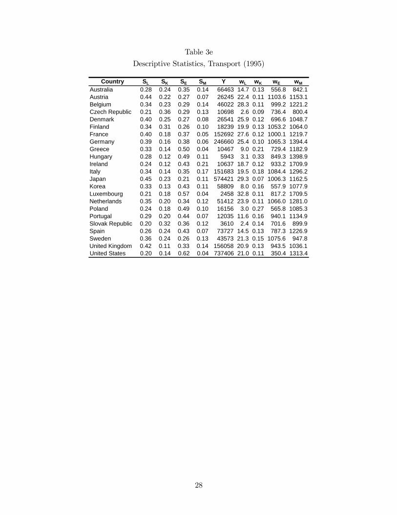
Table 3e

Descriptive Statistics, Transport (1995)

Country SL SK SE SM Y wL wK wE wM

Australia 0.28 0.24 0.35 0.14 66463 14.7 0.13 556.8 842.1Austria 0.44 0.22 0.27 0.07 26245 22.4 0.11 1103.6 1153.1Belgium 0.34 0.23 0.29 0.14 46022 28.3 0.11 999.2 1221.2Czech Republic 0.21 0.36 0.29 0.13 10698 2.6 0.09 736.4 800.4Denmark 0.40 0.25 0.27 0.08 26541 25.9 0.12 696.6 1048.7Finland 0.34 0.31 0.26 0.10 18239 19.9 0.13 1053.2 1064.0France 0.40 0.18 0.37 0.05 152692 27.6 0.12 1000.1 1219.7Germany 0.39 0.16 0.38 0.06 246660 25.4 0.10 1065.3 1394.4Greece 0.33 0.14 0.50 0.04 10467 9.0 0.21 729.4 1182.9Hungary 0.28 0.12 0.49 0.11 5943 3.1 0.33 849.3 1398.9Ireland 0.24 0.12 0.43 0.21 10637 18.7 0.12 933.2 1709.9Italy 0.34 0.14 0.35 0.17 151683 19.5 0.18 1084.4 1296.2Japan 0.45 0.23 0.21 0.11 574421 29.3 0.07 1006.3 1162.5Korea 0.33 0.13 0.43 0.11 58809 8.0 0.16 557.9 1077.9Luxembourg 0.21 0.18 0.57 0.04 2458 32.8 0.11 817.2 1709.5Netherlands 0.35 0.20 0.34 0.12 51412 23.9 0.11 1066.0 1281.0Poland 0.24 0.18 0.49 0.10 16156 3.0 0.27 565.8 1085.3Portugal 0.29 0.20 0.44 0.07 12035 11.6 0.16 940.1 1134.9Slovak Republic 0.20 0.32 0.36 0.12 3610 2.4 0.14 701.6 899.9Spain 0.26 0.24 0.43 0.07 73727 14.5 0.13 787.3 1226.9Sweden 0.36 0.24 0.26 0.13 43573 21.3 0.15 1075.6 947.8United Kingdom 0.42 0.11 0.33 0.14 156058 20.9 0.13 943.5 1036.1United States 0.20 0.14 0.62 0.04 737406 21.0 0.11 350.4 1313.4

28

Table 4a29

Parameter Estimates: Total Cost Function (Economy Level)

est.coefficient

standarderror

est.coefficient

standarderror

Labor Share Equation: constant 1.170*** 0.115 0.737*** 0.092Labor Share Equation: Output ­0.028*** 0.008 0.004 0.005Labor Share Equation: Wage 0.134*** 0.013 0.130*** 0.015Labor Share Equation: Return on Capital 0.012*** 0.003 ­0.001 0.003Labor Share Equation: Energy Price ­0.053*** 0.010 ­0.041*** 0.012Labor Share Equation: Materials Price ­0.042*** 0.007 ­0.071*** 0.010Capital Share Equation: constant ­0.623*** 0.090 ­0.248*** 0.067Capital Share Equation: Output 0.060*** 0.006 0.036*** 0.004Capital Share Equation: Wage ­0.061*** 0.010 ­0.068*** 0.011Capital Share Equation: Return on Capital ­0.023*** 0.003 ­0.006** 0.002Capital Share Equation: Energy Price ­0.026*** 0.008 ­0.034*** 0.009Capital Share Equation: Materials Price 0.026*** 0.006 0.046*** 0.007Energy Share Equation: constant ­0.006 0.031 ­0.079*** 0.022Energy Share Equation: Output ­0.003 0.002 ­0.003** 0.001Energy Share Equation: Wage ­0.025*** 0.003 ­0.047*** 0.003Energy Share Equation: Return on Capital ­0.001 0.001 ­0.004*** 0.001Energy Share Equation: Energy Price 0.035*** 0.003 0.046*** 0.003Energy Share Equation: Materials Price ­0.003 0.002 0.004* 0.002Materials Share Equation: constant 0.459*** 0.126 0.590*** 0.098Materials Share Equation: Output ­0.028*** 0.008 ­0.037*** 0.006Materials Share Equation: Wage ­0.048*** 0.014 ­0.015 0.016Materials Share Equation: Return on Capital 0.012*** 0.004 0.011*** 0.004Materials Share Equation: Energy Price 0.045*** 0.011 0.029** 0.013Materials Share Equation: Materials Price 0.019** 0.008 0.021** 0.010Number of observationsLabor Share Equation: R2

Capital Share Equation: R2

Energy Share Equation: R2

Materials Share Equation: R2

LR Test: γL=γE=γM=η=0, χ2 (pval)note:  *** p<0.01, ** p<0.05, * p<0.1

0.94

 91.40 (0.00)

0.940.900.940.95

Restricted Model Unrestricted Model

3510.93

351

0.88

0.94

29Estimates for country-speci�c �xed e¤ects are not reported in Tables 4a-4e, and are available uponrequest.

29

Table 4b

Parameter Estimates: Total Cost Function (Agriculture)

est.coefficient

standarderror

est.coefficient

standarderror

Labor Share Equation: constant 1.183*** 0.193 1.061*** 0.162Labor Share Equation: Output ­0.083*** 0.019 ­0.081*** 0.013Labor Share Equation: Wage 0.101*** 0.011 0.111*** 0.009Labor Share Equation: Return on Capital 0.041*** 0.009 0.010 0.008Labor Share Equation: Energy Price ­0.033** 0.013 ­0.030*** 0.010Labor Share Equation: Materials Price 0.027 0.018 0.029*** 0.011Capital Share Equation: constant ­1.243*** 0.252 ­0.891*** 0.211Capital Share Equation: Output 0.179*** 0.025 0.134*** 0.016Capital Share Equation: Wage ­0.120*** 0.014 ­0.129*** 0.011Capital Share Equation: Return on Capital ­0.050*** 0.011 ­0.000 0.011Capital Share Equation: Energy Price 0.022 0.017 0.047*** 0.013Capital Share Equation: Materials Price ­0.100*** 0.023 ­0.079*** 0.014Energy Share Equation: constant 0.224** 0.095 0.017 0.097Energy Share Equation: Output ­0.069*** 0.009 ­0.025*** 0.007Energy Share Equation: Wage ­0.010* 0.005 ­0.018*** 0.005Energy Share Equation: Return on Capital ­0.017*** 0.004 ­0.026*** 0.005Energy Share Equation: Energy Price 0.006 0.006 ­0.011* 0.006Energy Share Equation: Materials Price 0.093*** 0.009 0.059*** 0.007Materials Share Equation: constant 0.836*** 0.155 0.812*** 0.147Materials Share Equation: Output ­0.027* 0.015 ­0.028** 0.011Materials Share Equation: Wage 0.029*** 0.009 0.036*** 0.008Materials Share Equation: Return on Capital 0.026*** 0.007 0.017** 0.007Materials Share Equation: Energy Price 0.004 0.011 ­0.006 0.009Materials Share Equation: Materials Price ­0.019 0.014 ­0.009 0.010Number of observationsLabor Share Equation: R2

Capital Share Equation: R2

Energy Share Equation: R2

Materials Share Equation: R2

LR Test: γL=γE=γM=η=0, χ2 (pval)note:  *** p<0.01, ** p<0.05, * p<0.1

0.92

67.03 (0.00)

0.940.860.850.87

Restricted Model Unrestricted Model

3430.91

343

0.82

0.91

30

Table 4c

Parameter Estimates: Total Cost Function (Commerce)30

est.coefficient

standarderror

est.coefficient

standarderror

Labor Share Equation: constant 3.953*** 0.190 3.185*** 0.174Labor Share Equation: Output ­0.272*** 0.016 ­0.209*** 0.012Labor Share Equation: Wage 0.292*** 0.017 0.273*** 0.015Labor Share Equation: Return on Capital ­0.008 0.007 ­0.031*** 0.008Labor Share Equation: Energy Price ­0.001 0.010 0.025* 0.014Labor Share Equation: Materials Price ­0.044*** 0.013 ­0.081*** 0.012Capital Share Equation: constant ­1.846*** 0.214 ­1.280*** 0.192Capital Share Equation: Output 0.190*** 0.018 0.149*** 0.013Capital Share Equation: Wage ­0.178*** 0.019 ­0.181*** 0.017Capital Share Equation: Return on Capital 0.005 0.008 0.026*** 0.009Capital Share Equation: Energy Price ­0.013 0.011 ­0.028* 0.015Capital Share Equation: Materials Price ­0.004 0.015 0.018 0.013Energy Share Equation: constant ­0.297*** 0.082 ­0.270*** 0.076Energy Share Equation: Output 0.023*** 0.007 0.025*** 0.005Energy Share Equation: Wage 0.009 0.007 0.010 0.007Energy Share Equation: Return on Capital 0.018*** 0.003 0.015*** 0.004Energy Share Equation: Energy Price ­0.007* 0.004 ­0.018*** 0.006Energy Share Equation: Materials Price 0.009 0.006 0.009* 0.005Materials Share Equation: constant ­0.758*** 0.170 ­0.634*** 0.178Materials Share Equation: Output 0.064*** 0.014 0.035*** 0.012Materials Share Equation: Wage ­0.100*** 0.015 ­0.101*** 0.016Materials Share Equation: Return on Capital ­0.007 0.007 ­0.011 0.008Materials Share Equation: Energy Price 0.034*** 0.009 0.021 0.014Materials Share Equation: Materials Price 0.002 0.012 0.055*** 0.013Number of observationsLabor Share Equation: R2

Capital Share Equation: R2

Energy Share Equation: R2

Materials Share Equation: R2

LR Test: γL=γE=γM=η=0, χ2 (pval)note:  *** p<0.01, ** p<0.05, * p<0.1

0.87

25.85 (0.01)

0.890.730.830.86

Restricted Model Unrestricted Model

3300.94

330

0.72

0.94

30Korea was excluded from the sample due to large measurement error in capital stock.

31

Table 4d

Parameter Estimates: Total Cost Function (Manufacturing)

est.coefficient

standarderror

est.coefficient

standarderror

Labor Share Equation: constant 1.125*** 0.086 1.055*** 0.072Labor Share Equation: Output ­0.065*** 0.006 ­0.068*** 0.005Labor Share Equation: Wage 0.049*** 0.007 0.082*** 0.007Labor Share Equation: Return on Capital 0.021*** 0.003 0.009** 0.004Labor Share Equation: Energy Price 0.019*** 0.006 0.017*** 0.006Labor Share Equation: Materials Price ­0.010 0.007 ­0.010* 0.006Capital Share Equation: constant ­1.050*** 0.090 ­0.837*** 0.083Capital Share Equation: Output 0.104*** 0.007 0.091*** 0.006Capital Share Equation: Wage ­0.058*** 0.007 ­0.079*** 0.008Capital Share Equation: Return on Capital ­0.013*** 0.003 ­0.001 0.004Capital Share Equation: Energy Price ­0.020*** 0.007 ­0.017** 0.007Capital Share Equation: Materials Price ­0.013* 0.007 ­0.007 0.007Energy Share Equation: constant 0.626*** 0.091 0.388*** 0.089Energy Share Equation: Output ­0.069*** 0.007 ­0.048*** 0.006Energy Share Equation: Wage 0.024*** 0.007 0.013 0.009Energy Share Equation: Return on Capital ­0.010*** 0.003 ­0.018*** 0.004Energy Share Equation: Energy Price ­0.034*** 0.007 ­0.034*** 0.008Energy Share Equation: Materials Price 0.091*** 0.007 0.083*** 0.007Materials Share Equation: constant 0.299** 0.145 0.395*** 0.136Materials Share Equation: Output 0.030*** 0.011 0.025*** 0.010Materials Share Equation: Wage ­0.015 0.012 ­0.016 0.014Materials Share Equation: Return on Capital 0.002 0.006 0.011 0.007Materials Share Equation: Energy Price 0.035*** 0.011 0.033*** 0.012Materials Share Equation: Materials Price ­0.068*** 0.011 ­0.066*** 0.011Number of observationsLabor Share Equation: R2

Capital Share Equation: R2

Energy Share Equation: R2

Materials Share Equation: R2

LR Test: γL=γE=γM=η=0, χ2 (pval)note:  *** p<0.01, ** p<0.05, * p<0.1

0.91

27.51 (0.006)

0.910.870.830.83

Restricted Model Unrestricted Model

3460.95

346

0.88

0.94

32

Table 4e

Parameter Estimates: Total Cost Function (Transport)

est.coefficient

standarderror

est.coefficient

standarderror

Labor Share Equation: constant 1.515*** 0.108 1.191*** 0.108Labor Share Equation: Output ­0.085*** 0.009 ­0.055*** 0.005Labor Share Equation: Wage 0.139*** 0.012 0.177*** 0.011Labor Share Equation: Return on Capital 0.029*** 0.005 0.006 0.005Labor Share Equation: Energy Price 0.013 0.010 0.031*** 0.011Labor Share Equation: Materials Price ­0.084*** 0.009 ­0.135*** 0.011Capital Share Equation: constant ­0.889*** 0.139 ­0.639*** 0.151Capital Share Equation: Output 0.076*** 0.011 0.044*** 0.008Capital Share Equation: Wage ­0.115*** 0.015 ­0.114*** 0.016Capital Share Equation: Return on Capital ­0.055*** 0.007 ­0.043*** 0.006Capital Share Equation: Energy Price 0.035*** 0.013 0.044*** 0.016Capital Share Equation: Materials Price 0.005 0.012 0.021 0.015Energy Share Equation: constant 0.666*** 0.122 0.538*** 0.132Energy Share Equation: Output ­0.032*** 0.010 ­0.015** 0.007Energy Share Equation: Wage ­0.010 0.014 ­0.062*** 0.014Energy Share Equation: Return on Capital 0.009 0.006 0.021*** 0.006Energy Share Equation: Energy Price ­0.052*** 0.011 ­0.068*** 0.014Energy Share Equation: Materials Price 0.101*** 0.010 0.135*** 0.013Materials Share Equation: constant ­0.291*** 0.096 ­0.090 0.104Materials Share Equation: Output 0.041*** 0.008 0.026*** 0.005Materials Share Equation: Wage ­0.014 0.011 ­0.0004 0.011Materials Share Equation: Return on Capital 0.017*** 0.005 0.017*** 0.004Materials Share Equation: Energy Price 0.004 0.009 ­0.006 0.011Materials Share Equation: Materials Price ­0.022*** 0.008 ­0.021** 0.011Number of observationsLabor Share Equation: R2

Capital Share Equation: R2

Energy Share Equation: R2

Materials Share Equation: R2

LR Test: γL=γE=γM=η=0, χ2 (pval)note:  *** p<0.01, ** p<0.05, * p<0.1

0.89

63.95 (0.00)

0.890.960.840.85

Restricted Model Unrestricted Model

3460.94

346

0.96

0.93

33

Table 5a

Estimated Energy Demand Elasticities by Country (Economy Level)

Countrymean sd mean sd mean sd mean sd

Australia ­0.08 0.038 ­0.05 0.004 ­0.08 0.007 0.15 0.006Austria 0.06 0.072 ­0.05 0.004 ­0.11 0.007 0.14 0.004Belgium ­0.12 0.038 ­0.05 0.002 ­0.11 0.006 0.14 0.003Czech Republic ­0.24 0.027 ­0.08 0.003 ­0.11 0.010 0.13 0.003Denmark 0.16 0.084 ­0.05 0.003 ­0.12 0.005 0.14 0.003Finland ­0.12 0.051 ­0.05 0.010 ­0.13 0.025 0.14 0.005France ­0.02 0.046 ­0.04 0.003 ­0.10 0.006 0.15 0.004Germany ­0.04 0.059 ­0.04 0.003 ­0.11 0.006 0.15 0.004Greece ­0.20 0.042 ­0.04 0.007 ­0.05 0.013 0.17 0.017Hungary ­0.33 0.037 ­0.05 0.017 ­0.11 0.034 0.15 0.008Ireland 0.02 0.125 ­0.07 0.013 ­0.09 0.015 0.13 0.008Italy ­0.13 0.036 ­0.05 0.006 ­0.12 0.018 0.14 0.004Japan 0.13 0.036 ­0.07 0.004 ­0.08 0.009 0.13 0.006Korea ­0.15 0.127 ­0.05 0.007 ­0.19 0.042 0.13 0.012Luxembourg ­0.29 0.050 ­0.03 0.010 ­0.04 0.012 0.20 0.020Netherlands ­0.04 0.057 ­0.05 0.005 ­0.12 0.008 0.14 0.008Poland ­0.19 0.043 ­0.04 0.004 ­0.17 0.022 0.14 0.004Portugal ­0.16 0.058 ­0.05 0.008 ­0.13 0.019 0.14 0.009Slovak Republic ­0.32 0.029 ­0.09 0.006 ­0.06 0.007 0.14 0.005Spain ­0.01 0.049 ­0.06 0.004 ­0.11 0.011 0.13 0.006Sweden ­0.15 0.039 ­0.04 0.005 ­0.11 0.014 0.15 0.005United Kingdom ­0.11 0.050 ­0.03 0.005 ­0.13 0.009 0.15 0.005United States ­0.05 0.083 ­0.03 0.005 ­0.08 0.007 0.18 0.011

ηKE ηMEηEE ηLE

Table 5b

Estimated Energy Demand Elasticities by Country (Agriculture)

Countrymean sd mean sd mean sd mean sd

Australia ­1.04 0.02 ­0.01 0.02 0.31 0.08 0.07 0.008Austria ­1.04 0.02 0.03 0.01 12.12 24.85 0.07 0.006Belgium ­0.94 0.06 0.04 0.04 0.45 0.08 0.13 0.036Czech Republic ­1.11 0.17 ­0.02 0.06 0.35 0.10 0.07 0.068Denmark ­0.95 0.03 0.02 0.02 0.59 0.71 0.12 0.017Finland ­0.99 0.02 0.04 0.01 0.96 0.56 0.09 0.012France ­1.16 0.02 ­0.02 0.01 1.01 1.37 0.04 0.003Germany ­1.03 0.03 0.03 0.01 5.02 10.36 0.07 0.011Greece ­1.01 0.02 0.04 0.01 0.55 0.33 0.08 0.006Hungary ­0.96 0.03 0.00 0.03 0.42 0.07 0.12 0.015Ireland ­1.09 0.02 ­0.01 0.02 0.64 0.34 0.05 0.005Italy ­1.04 0.03 0.03 0.01 4.63 14.99 0.06 0.010Japan ­1.09 0.03 ­0.04 0.01 0.23 0.02 0.05 0.009Korea ­1.05 0.07 0.04 0.03 0.96 1.05 0.05 0.031Luxembourg ­3.31 0.42 ­0.06 0.01 1.23 1.42 ­0.01 0.002Netherlands ­0.85 0.02 0.12 0.02 4.88 13.33 0.19 0.015Poland ­1.04 0.07 0.02 0.03 0.23 0.05 0.04 0.038Portugal ­1.07 0.05 0.02 0.02 1.94 3.47 0.05 0.018Slovak Republic ­1.09 0.08 ­0.08 0.03 0.29 0.08 0.06 0.024Spain ­1.08 0.05 ­0.03 0.01 0.21 0.02 0.05 0.016Sweden ­1.01 0.03 0.03 0.01 0.43 0.08 0.08 0.012United Kingdom ­1.34 0.06 ­0.05 0.01 0.40 0.12 0.01 0.004United States ­1.06 0.05 ­0.03 0.02 0.27 0.05 0.06 0.018

ηEE ηLE ηKE ηME

34

Table 5c

Estimated Energy Demand Elasticities by Country (Commerce)31

Countrymean sd mean sd mean sd mean sd

Australia ­1.29 0.092 0.10 0.014 ­0.10 0.016 0.15 0.014Austria ­1.66 0.066 0.08 0.004 ­0.08 0.006 0.14 0.008Belgium ­1.34 0.196 0.11 0.018 ­0.05 0.029 0.17 0.054Czech Republic ­1.33 0.143 0.10 0.024 ­0.07 0.036 0.15 0.034Denmark ­1.53 0.042 0.07 0.002 ­0.13 0.022 0.17 0.005Finland ­1.34 0.096 0.10 0.016 ­0.12 0.068 0.14 0.013France ­1.29 0.032 0.09 0.005 ­0.09 0.028 0.23 0.010Germany ­1.62 0.127 0.06 0.006 ­0.20 0.035 0.25 0.016Greece ­1.65 0.081 0.09 0.009 ­0.04 0.008 0.19 0.019Hungary ­1.17 0.161 0.14 0.050 ­0.05 0.044 0.20 0.085Ireland ­1.77 0.475 0.07 0.015 ­0.07 0.028 0.28 0.039Italy ­1.32 0.064 0.10 0.006 ­0.12 0.017 0.14 0.024Japan ­2.23 0.051 0.06 0.001 ­0.08 0.007 0.19 0.014Luxembourg ­1.75 0.118 0.07 0.004 ­0.05 0.004 0.33 0.027Netherlands ­2.06 0.095 0.06 0.003 ­0.11 0.023 0.16 0.013Poland ­1.32 0.057 0.14 0.009 ­0.02 0.005 0.13 0.006Portugal ­1.34 0.131 0.09 0.017 ­0.10 0.029 0.16 0.017Slovak Republic ­1.27 0.073 0.13 0.030 ­0.04 0.021 0.14 0.010Spain ­1.41 0.059 0.09 0.005 ­0.07 0.009 0.18 0.012Sweden ­1.49 0.033 0.07 0.001 ­0.15 0.066 0.29 0.026United Kingdom ­1.47 0.098 0.08 0.009 ­0.10 0.017 0.16 0.012United States ­1.51 0.048 0.07 0.003 ­0.09 0.017 0.22 0.009

ηEE ηLE ηKE ηME

Table 5d

Estimated Energy Demand Elasticities by Country (Manufacturing)

Countrymean sd mean sd mean sd mean sd

Australia ­1.18 0.04 0.19 0.01 ­0.02 0.01 0.18 0.01Austria ­1.41 0.04 0.14 0.01 ­0.06 0.02 0.13 0.01Belgium ­1.20 0.04 0.19 0.01 ­0.05 0.01 0.17 0.01Czech Republic ­1.33 0.17 0.20 0.03 ­0.06 0.04 0.14 0.04Denmark ­1.63 0.08 0.11 0.01 ­0.11 0.02 0.11 0.01Finland ­1.31 0.09 0.17 0.01 ­0.03 0.02 0.15 0.02France ­1.40 0.04 0.15 0.01 ­0.10 0.01 0.13 0.01Germany ­1.33 0.04 0.14 0.01 ­0.10 0.02 0.15 0.01Greece ­1.21 0.10 0.17 0.02 ­0.06 0.06 0.17 0.03Hungary ­1.11 0.14 0.26 0.04 ­0.04 0.05 0.21 0.06Ireland ­1.45 0.16 0.19 0.01 0.00 0.00 0.14 0.02Italy ­1.39 0.04 0.15 0.01 ­0.10 0.01 0.13 0.01Japan ­1.57 0.08 0.13 0.01 ­0.04 0.01 0.12 0.01Korea ­1.21 0.03 0.21 0.01 ­0.05 0.02 0.16 0.01Luxembourg ­1.01 0.04 0.27 0.02 0.02 0.03 0.24 0.02Netherlands ­1.16 0.03 0.20 0.01 ­0.03 0.01 0.18 0.01Poland ­1.10 0.13 0.25 0.04 ­0.02 0.04 0.21 0.05Portugal ­1.26 0.03 0.19 0.01 ­0.07 0.01 0.15 0.01Slovak Republic ­1.10 0.11 0.27 0.04 0.02 0.04 0.21 0.05Spain ­1.26 0.07 0.18 0.01 ­0.04 0.01 0.16 0.01Sweden ­1.45 0.07 0.13 0.01 ­0.07 0.03 0.13 0.01United Kingdom ­1.44 0.07 0.12 0.01 ­0.10 0.03 0.13 0.01United States ­1.11 0.05 0.20 0.02 0.02 0.01 0.22 0.02

ηEE ηLE ηKE ηME

31The results for Korea are not reported (see footnote above).

35

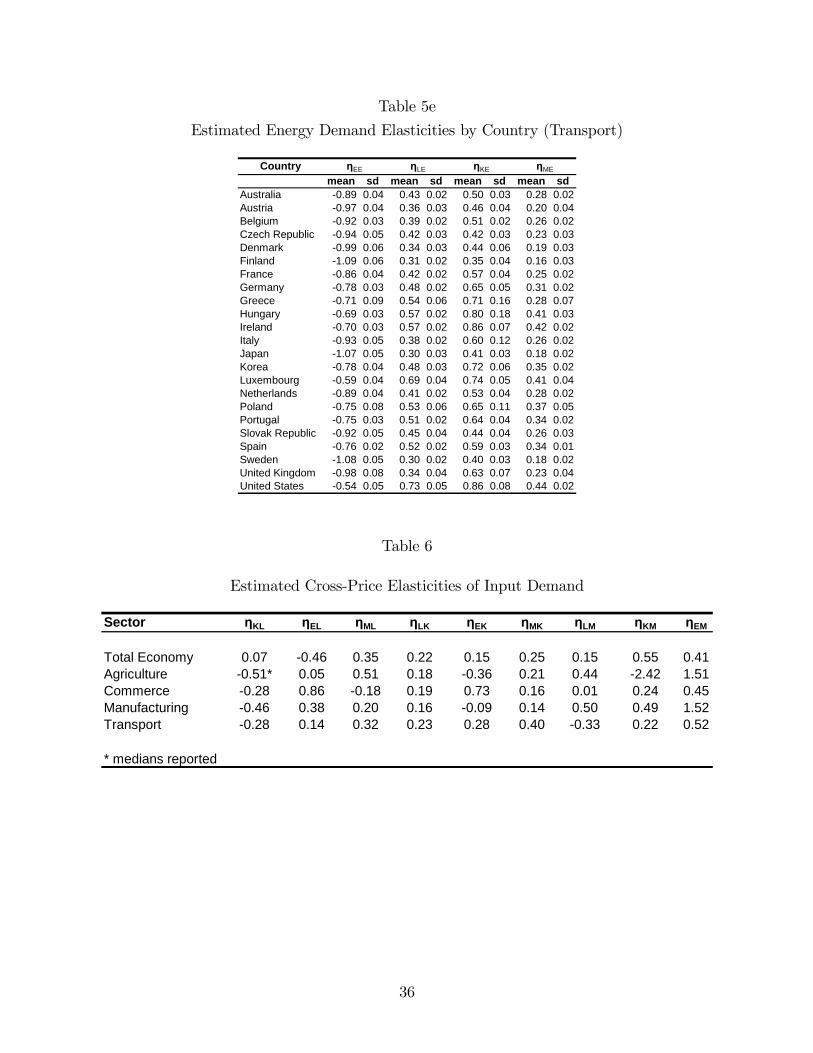
Table 5e

Estimated Energy Demand Elasticities by Country (Transport)

Countrymean sd mean sd mean sd mean sd

Australia ­0.89 0.04 0.43 0.02 0.50 0.03 0.28 0.02Austria ­0.97 0.04 0.36 0.03 0.46 0.04 0.20 0.04Belgium ­0.92 0.03 0.39 0.02 0.51 0.02 0.26 0.02Czech Republic ­0.94 0.05 0.42 0.03 0.42 0.03 0.23 0.03Denmark ­0.99 0.06 0.34 0.03 0.44 0.06 0.19 0.03Finland ­1.09 0.06 0.31 0.02 0.35 0.04 0.16 0.03France ­0.86 0.04 0.42 0.02 0.57 0.04 0.25 0.02Germany ­0.78 0.03 0.48 0.02 0.65 0.05 0.31 0.02Greece ­0.71 0.09 0.54 0.06 0.71 0.16 0.28 0.07Hungary ­0.69 0.03 0.57 0.02 0.80 0.18 0.41 0.03Ireland ­0.70 0.03 0.57 0.02 0.86 0.07 0.42 0.02Italy ­0.93 0.05 0.38 0.02 0.60 0.12 0.26 0.02Japan ­1.07 0.05 0.30 0.03 0.41 0.03 0.18 0.02Korea ­0.78 0.04 0.48 0.03 0.72 0.06 0.35 0.02Luxembourg ­0.59 0.04 0.69 0.04 0.74 0.05 0.41 0.04Netherlands ­0.89 0.04 0.41 0.02 0.53 0.04 0.28 0.02Poland ­0.75 0.08 0.53 0.06 0.65 0.11 0.37 0.05Portugal ­0.75 0.03 0.51 0.02 0.64 0.04 0.34 0.02Slovak Republic ­0.92 0.05 0.45 0.04 0.44 0.04 0.26 0.03Spain ­0.76 0.02 0.52 0.02 0.59 0.03 0.34 0.01Sweden ­1.08 0.05 0.30 0.02 0.40 0.03 0.18 0.02United Kingdom ­0.98 0.08 0.34 0.04 0.63 0.07 0.23 0.04United States ­0.54 0.05 0.73 0.05 0.86 0.08 0.44 0.02

ηEE ηLE ηKE ηME

Table 6

Estimated Cross-Price Elasticities of Input Demand

Sector ηKL ηEL ηML ηLK ηEK ηMK ηLM ηKM ηEM

Total Economy 0.07 ­0.46 0.35 0.22 0.15 0.25 0.15 0.55 0.41Agriculture ­0.51* 0.05 0.51 0.18 ­0.36 0.21 0.44 ­2.42 1.51Commerce ­0.28 0.86 ­0.18 0.19 0.73 0.16 0.01 0.24 0.45Manufacturing ­0.46 0.38 0.20 0.16 ­0.09 0.14 0.50 0.49 1.52Transport ­0.28 0.14 0.32 0.23 0.28 0.40 ­0.33 0.22 0.52

* medians reported

36

Table 7

Greenhouse Gas Emissions in UK Manufacturing Sector in 2005

Fuel TypeFuel Consumption

(toe)Fuel

Share (%)CO2 Emission

per toeCO2 emission

per Share

Gas/Diesel Oil 3641939 0.09 2.90 0.25Motor Gasoline 0 0.00 2.82 0.00Naphtha 2074889 0.05 2.87 0.14Kerosene type Jet Fuel 0 0.00 2.81 0.00Residual Fuel Oil 763697 0.02 3.13 0.06Liquefied Petroleum Gases 3329969 0.08 2.50 0.20Other Petroleum Products 7177334 0.17 2.90 0.50Coal 1814070 0.04 3.70 0.16Natural gas 12786713 0.31 2.17 0.66Electricity 10219552 0.24 2.17* 0.53*Total 41808164 1.00 2.51

* Assuming Natural Gas as a Base Load Factor in Electricity Generation

37

Appendix III - Charts

Figure 1a

Capital Stock E¢ ciency Indexes, U.S. Economy, 1991-2005

0.600

0.700

0.800

0.900

1.000

1.100

1.200

1990 1991 1992 1993 1994 1995 1996 1997 1998 1999 2000 2001 2002 2003 2004 2005

Labor Energy Materials

Figure 1b

Capital Stock E¢ ciency Indexes, U.S. Agriculture Sector, 1991-2005

0.600

0.700

0.800

0.900

1.000

1.100

1.200

1.300

1.400

1.500

1.600

1991 1992 1993 1994 1995 1996 1997 1998 1999 2000 2001 2002 2003 2004 2005

Labor Energy Materials

38

Figure 1c

Capital Stock E¢ ciency Indexes, U.S. Commerce Sector, 1991-2005

0.600

0.700

0.800

0.900

1.000

1.100

1.200

1.300

1.400

1991 1992 1993 1994 1995 1996 1997 1998 1999 2000 2001 2002 2003 2004 2005

Labor Energy Materials

Figure 1d

Capital Stock E¢ ciency Indexes, U.S. Manufacturing Sector, 1991-2005

0.650

0.700

0.750

0.800

0.850

0.900

0.950

1.000

1.050

1.100

1991 1992 1993 1994 1995 1996 1997 1998 1999 2000 2001 2002 2003 2004 2005

Labor Energy Materials

39

Figure 1e

Capital Stock E¢ ciency Indexes, U.S. Transport Sector, 1991-2005

0.500

0.700

0.900

1.100

1.300

1.500

1.700

1.900

1991 1992 1993 1994 1995 1996 1997 1998 1999 2000 2001 2002 2003 2004 2005

Labor Energy Materials

40