Copyright © Cengage Learning. All rights reserved.

CHAPTER 8

RELATIONSRELATIONS

Copyright © Cengage Learning. All rights reserved.

Partial Order Relations

SECTION 8.5

3

Partial Order Relations

In order to obtain a degree in computer science at a certain

university, a student must take a specified set of required

courses, some of which must be completed before others

can be started.

Given the prerequisite structure of the program, one might ask what is the least number of school terms needed to

fulfill the degree requirements, or what is the maximum

number of courses that can be taken in the same term, or

whether there is a sequence in which a part-time student can take the courses one per term.

4

Antisymmetry

5

Antisymmetry

We have defined three properties of relations: reflexivity,

symmetry, and transitivity. A fourth property of relations is

called antisymmetry.

In terms of the arrow diagram of a relation, saying that a

relation is antisymmetric is the same as saying that whenever there is an arrow going from one element to

another distinct element, there is not an arrow going back

from the second to the first.

6

Antisymmetry

By taking the negation of the definition, you can see that a

relation R is not antisymmetric if, and only if,

there are elements a and b in A such that a R b and b R a

but a ≠≠≠≠ b.

7

Example 2 – Testing for Antisymmetry of “Divides” Relations

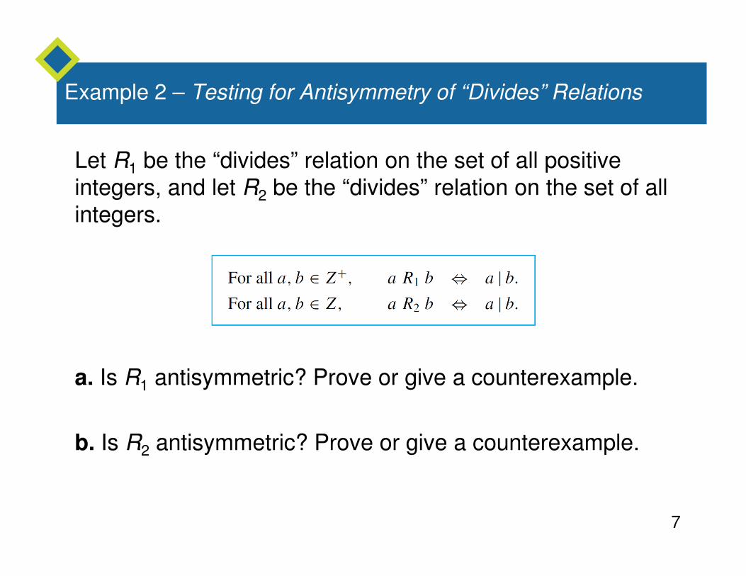
Let R1 be the “divides” relation on the set of all positive

integers, and let R2 be the “divides” relation on the set of all

integers.

a. Is R1 antisymmetric? Prove or give a counterexample.

b. Is R2 antisymmetric? Prove or give a counterexample.

8

Example 2 – Solution

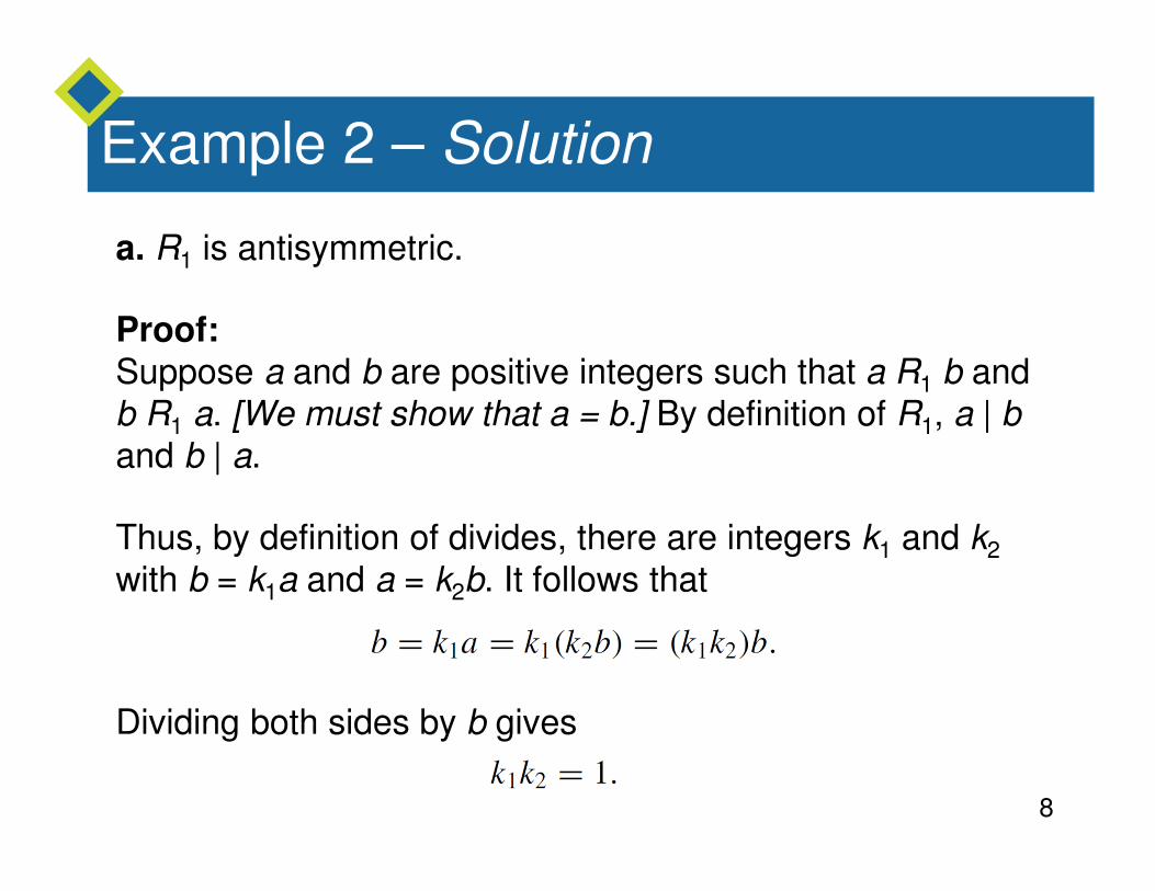
a. R1 is antisymmetric.

Proof:

Suppose a and b are positive integers such that a R1 b and

b R1 a. [We must show that a = b.] By definition of R1, a | b

and b | a.

Thus, by definition of divides, there are integers k1 and k2

with b = k1a and a = k2b. It follows that

Dividing both sides by b gives

9

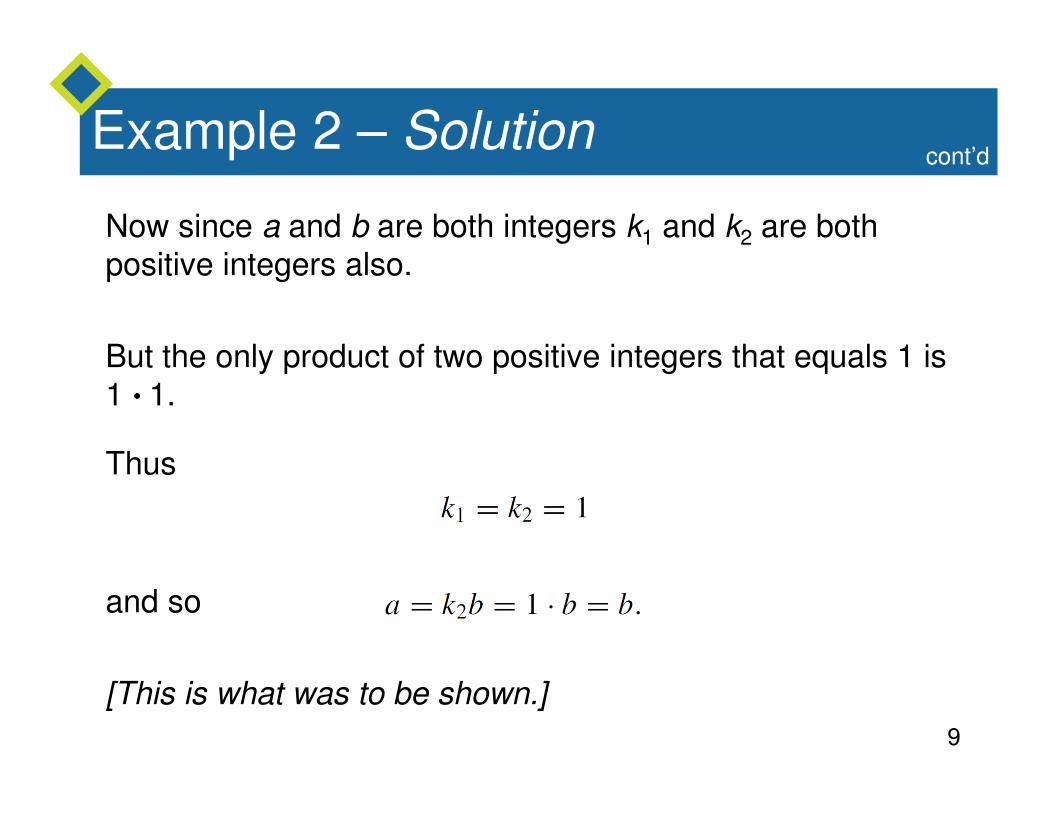
Example 2 – Solution

Now since a and b are both integers k1 and k2 are both

positive integers also.

But the only product of two positive integers that equals 1 is

1 ���� 1.

Thus

and so

[This is what was to be shown.]

cont’d

10

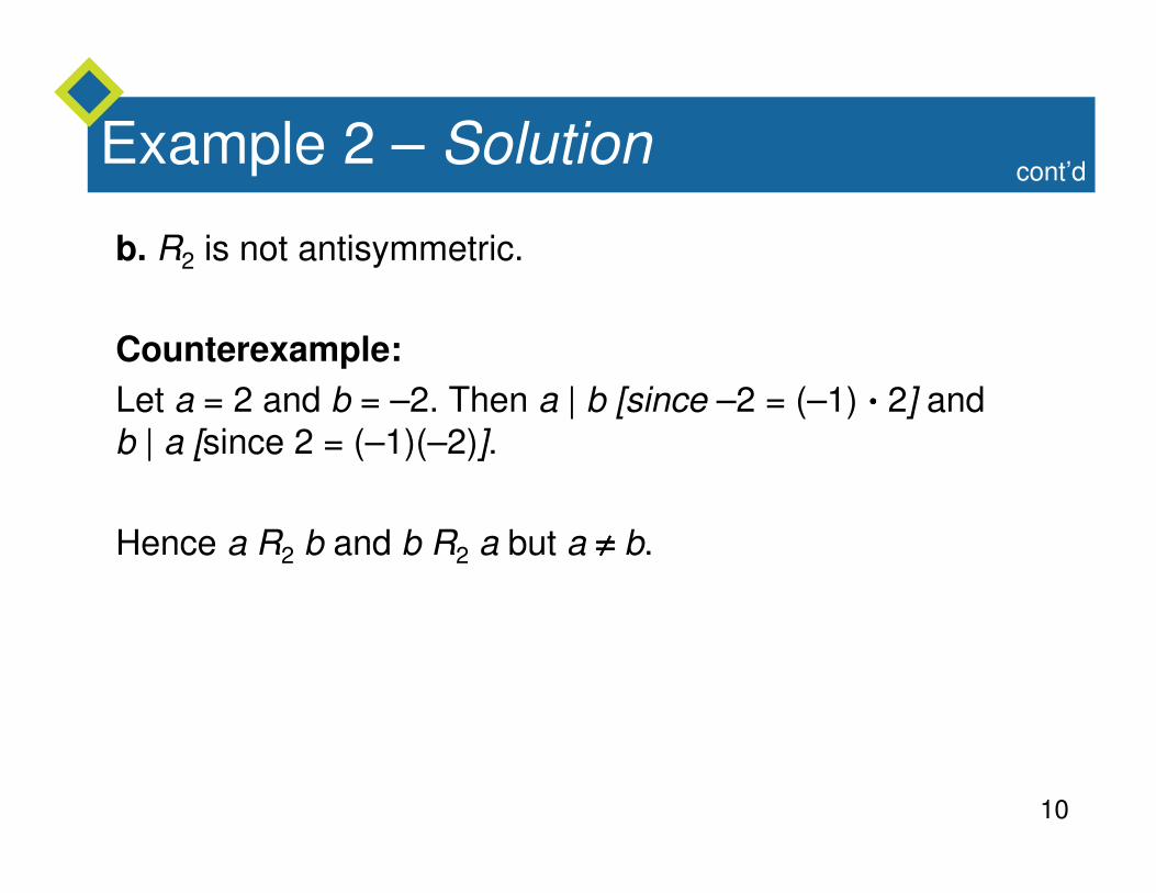
Example 2 – Solution

b. R2 is not antisymmetric.

Counterexample:

Let a = 2 and b = –2. Then a | b [since –2 = (–1) ���� 2] andb | a [since 2 = (–1)(–2)].

Hence a R2 b and b R2 a but a ≠≠≠≠ b.

cont’d

11

Partial Order Relations

12

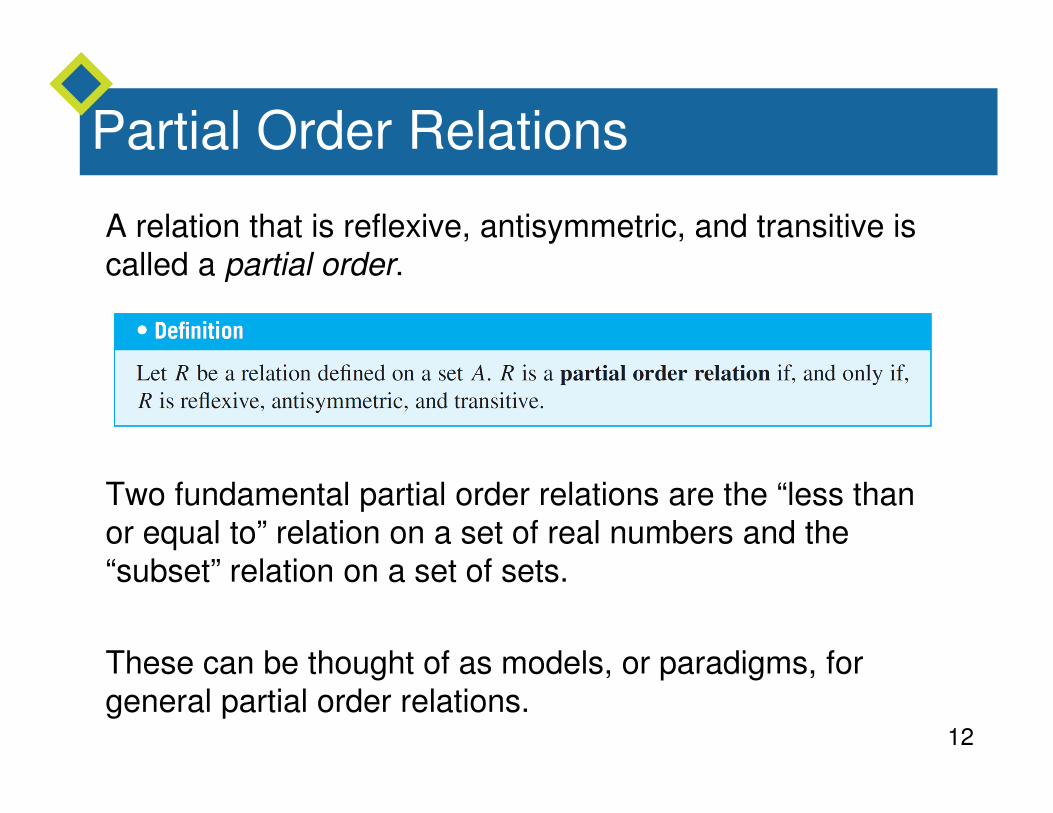
Partial Order Relations

A relation that is reflexive, antisymmetric, and transitive is

called a partial order.

Two fundamental partial order relations are the “less than

or equal to” relation on a set of real numbers and the “subset” relation on a set of sets.

These can be thought of as models, or paradigms, for general partial order relations.

13

Example 4 – A “Divides” Relation on a Set of Positive Integers

Let | be the “divides” relation on a set A of positive integers.

That is, for all a, b ∈ A,

Prove that | is a partial order relation on A.

Solution:

| is reflexive: [We must show that for all a ∈ A, a | a.]

Suppose a ∈ A. Then a = 1 ���� a, so a | a by definition of

divisibility.

14

Example 4 – Solution

| is antisymmetric: [We must show that for all a, b ∈ A, if

a | b and b | a then a = b.] The proof of this is virtually

identical to that of Example 2(a).

| is transitive: To show transitivity means to show that for all a, b, c ∈ A, if a | b and b | c then a | c. But this was

proved as Theorem 4.3.3.

Since | is reflexive, antisymmetric, and transitive, | is a partial order relation on A.

cont’d

15

Partial Order Relations

16

Lexicographic Order

17

Lexicographic Order

To figure out which of two words comes first in an English

dictionary, you compare their letters one by one from left to

right. If all letters have been the same to a certain point and

one word runs out of letters, that word comes first in the

dictionary.

For example, play comes before playhouse. If all letters up

to a certain point are the same and the next letters differ,

then the word whose next letter is located earlier in the

alphabet comes first in the dictionary. For instance, playhouse comes before playmate.

18

Lexicographic Order

More generally, if A is any set with a partial order relation,

then a dictionary or lexicographic order can be defined on a

set of strings over A as indicated in the following theorem.

19

Lexicographic Order

20

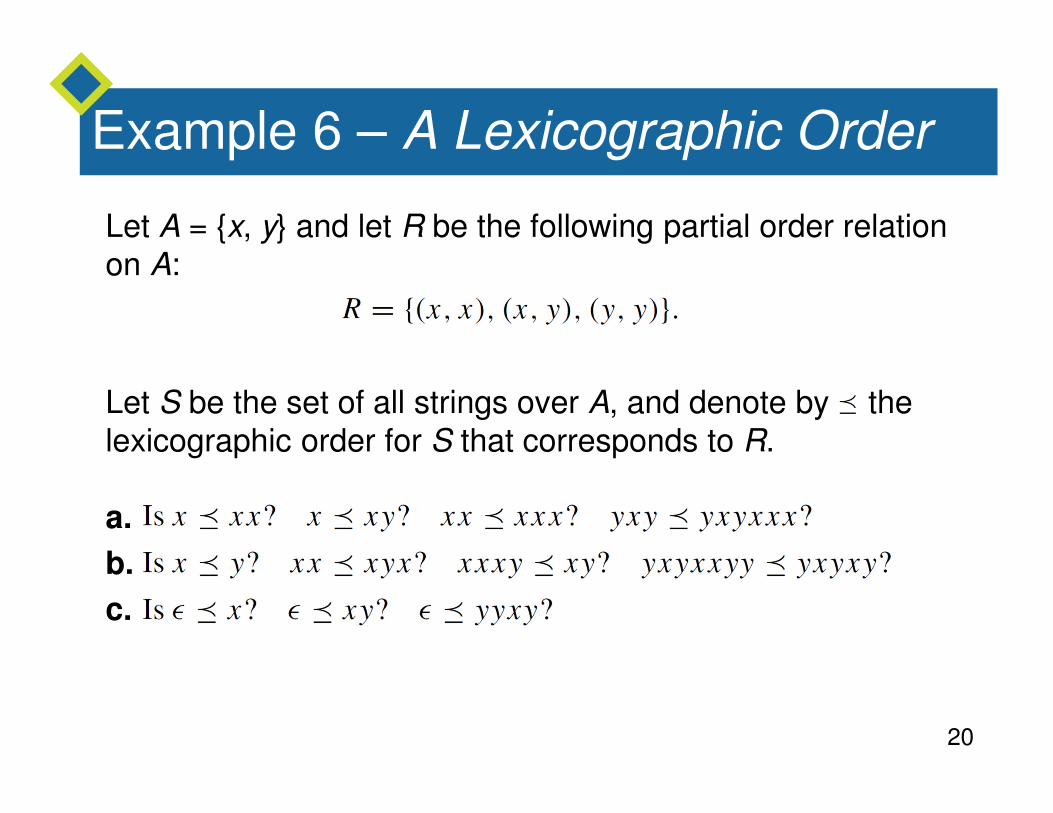
Example 6 – A Lexicographic Order

Let A = {x, y} and let R be the following partial order relation

on A:

Let S be the set of all strings over A, and denote by the

lexicographic order for S that corresponds to R.

a.

b.

c.

21

Example 6 – Solution

a. Yes in all cases, by relation (1) in theorem 8.5.1.

b. Yes in all cases, by relation (2) in theorem 8.5.1.

c. Yes in all cases, by relation (3) in theorem 8.5.1.

22

Hasse Diagrams

23

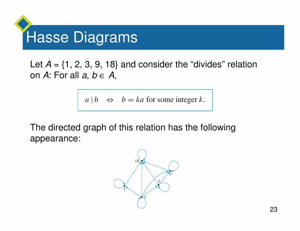
Hasse Diagrams

Let A = {1, 2, 3, 9, 18} and consider the “divides” relation

on A: For all a, b ∈ A,

The directed graph of this relation has the following

appearance:

24

Hasse Diagrams

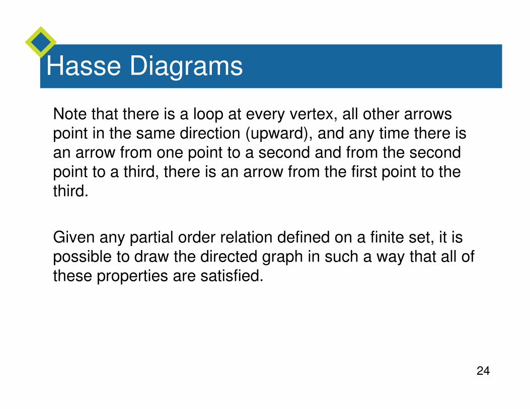
Note that there is a loop at every vertex, all other arrows

point in the same direction (upward), and any time there is

an arrow from one point to a second and from the second

point to a third, there is an arrow from the first point to the

third.

Given any partial order relation defined on a finite set, it is

possible to draw the directed graph in such a way that all of

these properties are satisfied.

25

Hasse Diagrams

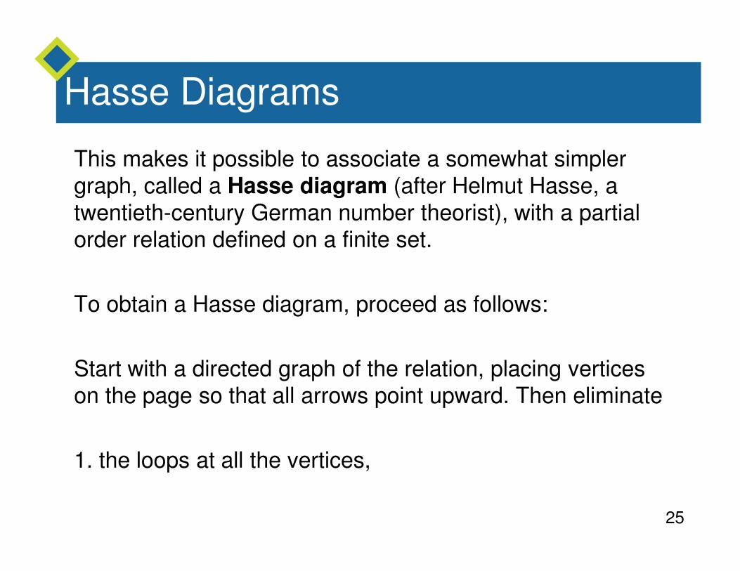
This makes it possible to associate a somewhat simpler

graph, called a Hasse diagram (after Helmut Hasse, a

twentieth-century German number theorist), with a partial

order relation defined on a finite set.

To obtain a Hasse diagram, proceed as follows:

Start with a directed graph of the relation, placing vertices

on the page so that all arrows point upward. Then eliminate

1. the loops at all the vertices,

26

Hasse Diagrams

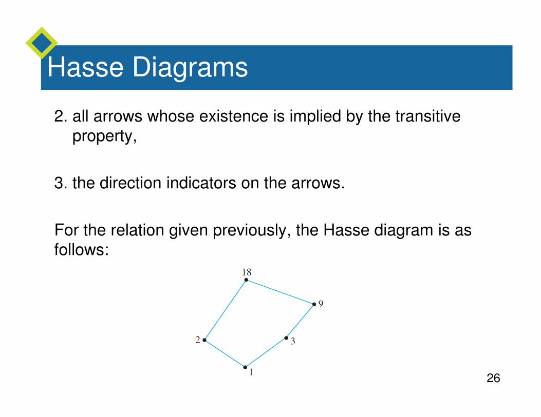
2. all arrows whose existence is implied by the transitive

property,

3. the direction indicators on the arrows.

For the relation given previously, the Hasse diagram is as

follows:

27

Example 7 – Constructing a Hasse Diagram

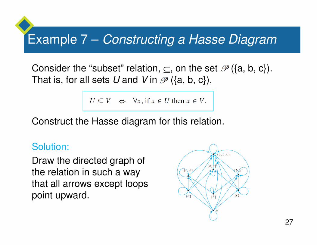
Consider the “subset” relation, ⊆, on the set ({a, b, c}).

That is, for all sets U and V in ({a, b, c}),

Construct the Hasse diagram for this relation.

Solution:

Draw the directed graph of the relation in such a way

that all arrows except loops

point upward.

28

Example 7 – Solution

Then strip away all loops, unnecessary arrows, and

direction indicators to obtain the Hasse diagram.

cont’d

29

Hasse Diagrams

To recover the directed graph of a relation from the Hasse

diagram, just reverse the instructions given previously,

using the knowledge that the original directed graph was

sketched so that all arrows pointed upward:

1. Reinsert the direction markers on the arrows making all arrows point upward.

2. Add loops at each vertex.

3. For each sequence of arrows from one point to a second

and from that second point to a third, add an arrow from the first point to the third.

30

Partially and Totally Ordered Sets

31

Partially and Totally Ordered Sets

Given any two real numbers x and y, either x ≤≤≤≤ y or y ≤≤≤≤ x. In

a situation like this, the elements x and y are said to be

comparable.

On the other hand, given two subsets A and B of {a, b, c}, it

may be the case that neither A ⊆ B nor B ⊆ A.

For instance, let A = {a, b} and B = {b, c}. Then and

In such a case, A and B are said to be noncomparable.

32

Partially and Totally Ordered Sets

When all the elements of a partial order relation are

comparable, the relation is called a total order.

33

Partially and Totally Ordered Sets

Both the “less than or equal to” relation on sets of real

numbers and the lexicographic order of the set of words in

a dictionary are total order relations.

Note that the Hasse diagram for a total order relation can

be drawn as a single vertical “chain.”

Many important partial order relations have elements that

are not comparable and are, therefore, not total order

relations.

34

Partially and Totally Ordered Sets

For instance, the subset relation on ({a, b, c}) is not a

total order relation because, as shown previously, the

subsets {a, b} and {a, c} of {a, b, c} are not comparable.

In addition, a “divides” relation is not a total order relation

unless the elements are all powers of a single integer.

A set A is called a partially ordered set (or poset) with

respect to a relation if, and only if, is a partial order

relation on A.

35

Partially and Totally Ordered Sets

For instance, the set of real numbers is a partially ordered

set with respect to the “less than or equal to” relation ≤≤≤≤, and

a set of sets is partially ordered with respect to the “subset”

relation ⊆.

It is entirely straightforward to show that any subset of a

partially ordered set is partially ordered.

This, of course, assumes the “same definition” for the

relation on the subset as for the set as a whole. A set A is called a totally ordered set with respect to a relation

if, and only if, A is partially ordered with respect to and is a total order.

36

Partially and Totally Ordered Sets

A set that is partially ordered but not totally ordered may

have totally ordered subsets. Such subsets are called

chains.

Observe that if B is a chain in A, then B is a totally ordered

set with respect to the “restriction” of to B.

37

Example 9 – A Chain of Subsets

The set is partially ordered with respect to the

subset relation. Find a chain of length 3 in

Solution:

Since the set

is a chain of length 3 in

38

Partially and Totally Ordered Sets

A maximal element in a partially ordered set is an element

that is greater than or equal to every element to which it is

comparable. (There may be many elements to which it is

not comparable.)

A greatest element in a partially ordered set is an element that is greater than or equal to every element in the set (so

it is comparable to every element in the set). Minimal and

least elements are defined similarly.

39

Partially and Totally Ordered Sets

40

Partially and Totally Ordered Sets

A greatest element is maximal, but a maximal element

need not be a greatest element. However, every finite

subset of a totally ordered set has both a least element and

a greatest element.

Similarly, a least element is minimal, but a minimal element need not be a least element. Furthermore, a set that is

partially ordered with respect to a relation can have at most

one greatest element and one least element, but it may

have more than one maximal or minimal element.

41

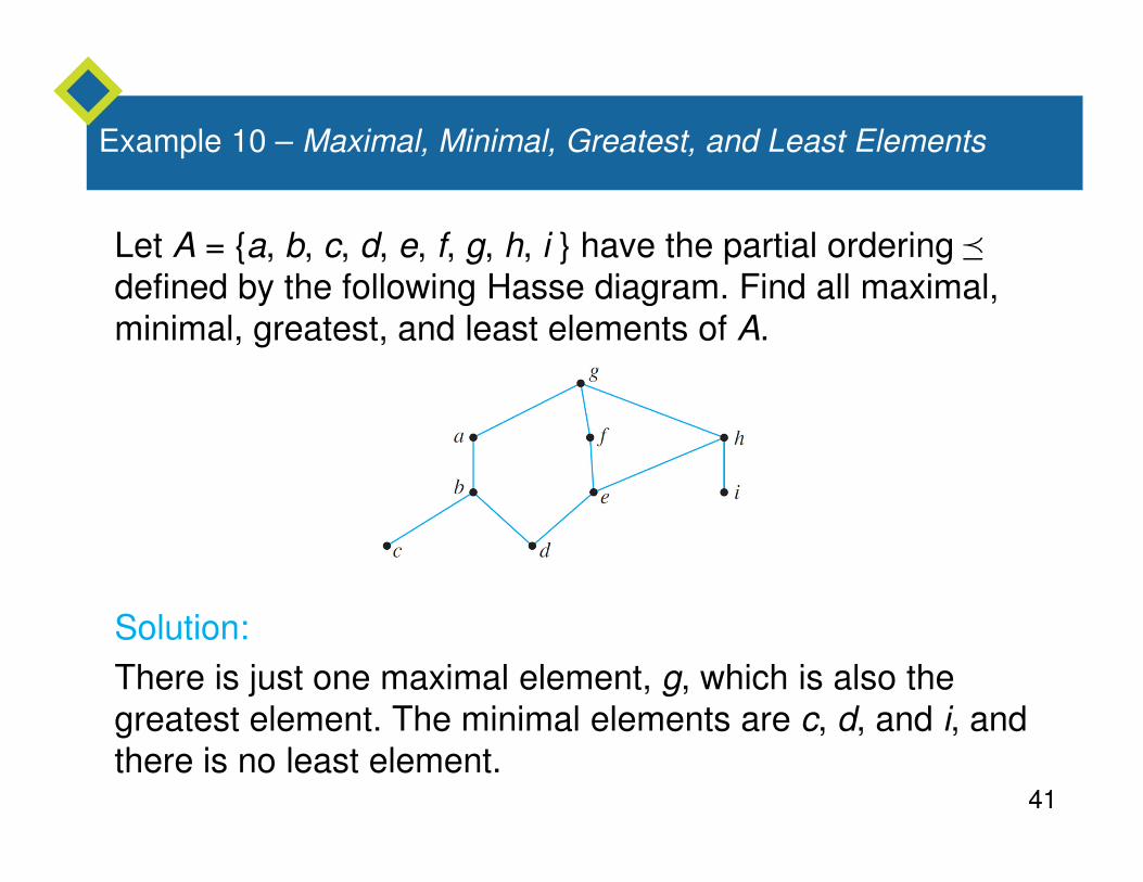
Example 10 – Maximal, Minimal, Greatest, and Least Elements

Let A = {a, b, c, d, e, f, g, h, i } have the partial ordering

defined by the following Hasse diagram. Find all maximal,

minimal, greatest, and least elements of A.

Solution:

There is just one maximal element, g, which is also the

greatest element. The minimal elements are c, d, and i, and

there is no least element.

42

Topological Sorting

43

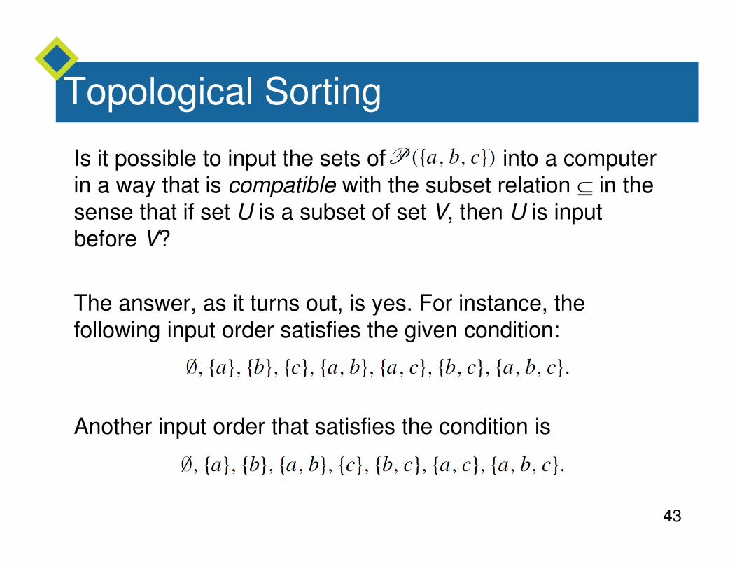
Topological Sorting

Is it possible to input the sets of into a computer

in a way that is compatible with the subset relation ⊆ in the

sense that if set U is a subset of set V, then U is input

before V?

The answer, as it turns out, is yes. For instance, the following input order satisfies the given condition:

Another input order that satisfies the condition is

44

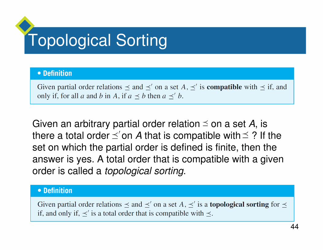
Topological Sorting

Given an arbitrary partial order relation on a set A, is

there a total order on A that is compatible with ? If the

set on which the partial order is defined is finite, then the answer is yes. A total order that is compatible with a given

order is called a topological sorting.

45

Topological Sorting

46

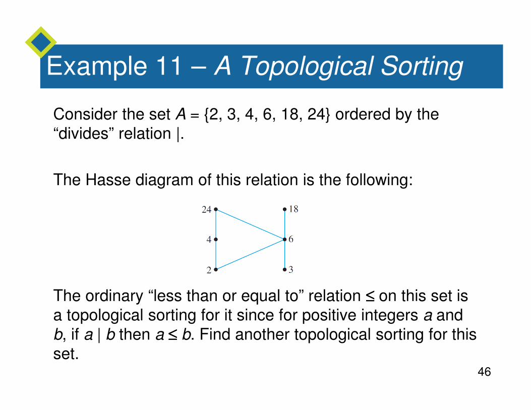
Example 11 – A Topological Sorting

Consider the set A = {2, 3, 4, 6, 18, 24} ordered by the

“divides” relation |.

The Hasse diagram of this relation is the following:

The ordinary “less than or equal to” relation ≤≤≤≤ on this set is a topological sorting for it since for positive integers a and

b, if a | b then a ≤≤≤≤ b. Find another topological sorting for this set.

47

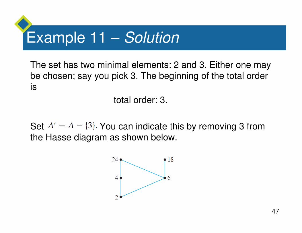
Example 11 – Solution

The set has two minimal elements: 2 and 3. Either one may

be chosen; say you pick 3. The beginning of the total order

is

total order: 3.

Set You can indicate this by removing 3 from

the Hasse diagram as shown below.

48

Example 11 – Solution

Next choose minimal element from . Only 2 is

minimal, so you must pick it. The total order thus far is

total order: 3 2.

Set .

You can indicate this by removing 2 from the Hasse

diagram, as is shown below.

Choose a minimal element from

cont’d

49

Example 11 – Solution

Again you have two choices: 4 and 6. Say you pick 6. The

total order for the elements chosen thus far is

total order: 3 2 6.

You continue in this way until every element of A has been

picked. One possible sequence of choices gives

total order: 3 2 6 18 4 24.

cont’d

50

Example 11 – Solution

You can verify that this order is compatible with the

“divides” partial order by checking that for each pair of

elements a and b in A such that a | b, then a b.

Note that it is not the case that if a b then a | b.

cont’d

51

An Application

52

An Application

To return to the example that introduced this section, note

that the following defines a partial order relation on the set

of courses required for a university degree: For all required

courses x and y,

If the Hasse diagram for the relation is drawn, then the

questions raised at the beginning of this section can be

answered easily.

53

An Application

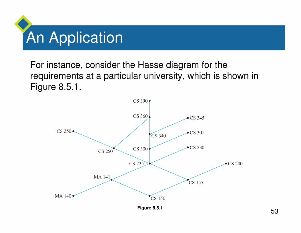
For instance, consider the Hasse diagram for the

requirements at a particular university, which is shown in

Figure 8.5.1.

Figure 8.5.1

54

An Application

The minimum number of school terms needed to complete

the requirements is the size of a longest chain, which is 7

(150, 155, 225, 300, 340, 360, 390, for example).

The maximum number of courses that could be taken in the

same term (assuming the university allows it) is the maximum number of noncomparable courses, which is 6

(350, 360, 345, 301, 230, 200, for example).

55

An Application

A part-time student could take the courses in a sequence

determined by constructing a topological sorting for the set.

(One such sorting is 140, 150, 141, 155, 200, 225, 230,

300, 250, 301, 340, 345, 350, 360, 390. There are many

others.)

56

PERT and CPM

57

PERT and CPM

Two important and widely used applications of partial order

relations are PERT (Program Evaluation and Review

Technique) and CPM (Critical Path Method).

These techniques came into being in the 1950s as

planners came to grips with the complexities of scheduling the individual activities needed to complete very large

projects, and although they are very similar, their

developments were independent.

58

PERT and CPM

PERT was developed by the U.S.

Navy to help organize the construction of the Polaris submarine, and CPM was developed by the E. I. Du Pont

de Nemours company for scheduling chemical plant

maintenance.

Here is a somewhat simplified example of the way the

techniques work.

59

Example 12 – A Job Scheduling Problem

At an automobile assembly plant, the job of assembling an

automobile can be broken down into these tasks:

1. Build frame.

2. Install engine, power train components, gas tank.

3. Install brakes, wheels, tires.

4. Install dashboard, floor, seats.

60

Example 12 – A Job Scheduling Problem

5. Install electrical lines.

6. Install gas lines.

7. Install brake lines.

8. Attach body panels to frame.

9. Paint body.

Certain of these tasks can be carried out at the same time,

whereas some cannot be started until other tasks are finished.

cont’d

61

Example 12 – A Job Scheduling Problem

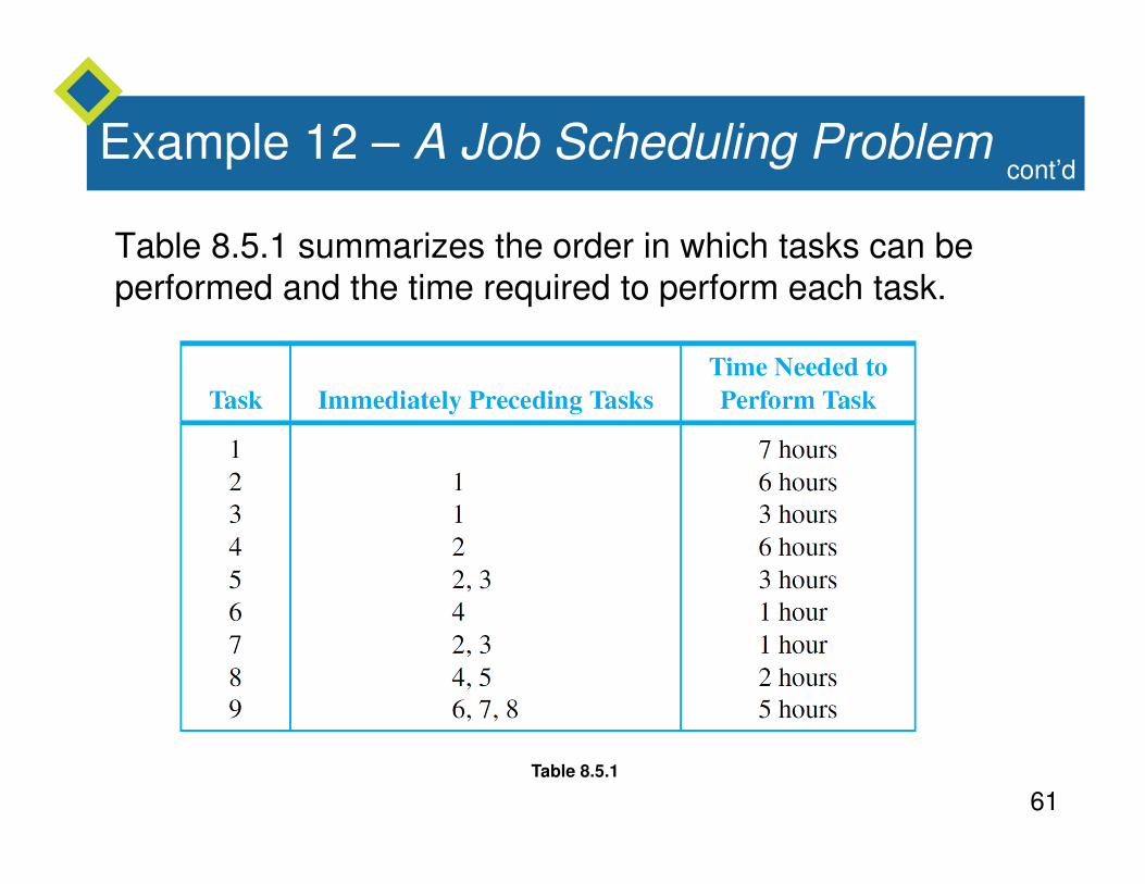
Table 8.5.1 summarizes the order in which tasks can be

performed and the time required to perform each task.

cont’d

Table 8.5.1

62

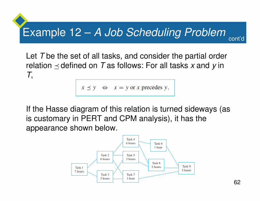
Example 12 – A Job Scheduling Problem

Let T be the set of all tasks, and consider the partial order

relation defined on T as follows: For all tasks x and y in

T,

If the Hasse diagram of this relation is turned sideways (as

is customary in PERT and CPM analysis), it has the appearance shown below.

cont’d

63

Example 12 – A Job Scheduling Problem

What is the minimum time required to assemble a car? You

can determine this by working from left to right across the

diagram, noting for each task (say, just above the box

representing that task) the minimum time needed to

complete that task starting from the beginning of the

assembly process.

For instance, you can put a 7 above the box for task 1 because task 1 requires 7 hours.

Task 2 requires completion of task 1 (7 hours) plus 6 hours for itself, so the minimum time required to complete task 2,

starting at the beginning of the assembly process, is 7 + 6 = 13 hours.

cont’d

64

Example 12 – A Job Scheduling Problem

You can put a 13 above the box for task 2.

Similarly, you can put a 10 above the box for task 3 because 7 + 3 = 10.

Now consider what number you should write above the box

for task 5.

The minimum times to complete tasks 2 and 3, starting

from the beginning of the assembly process, are 13 and 10

hours respectively.

cont’d

65

Example 12 – A Job Scheduling Problem

Since both tasks must be completed before task 5 can be

started, the minimum time to complete task 5, starting from

the beginning, is the time needed for task 5 itself (3 hours)

plus the maximum of the times to complete tasks 2 and 3

(13 hours), and this equals 3 + 13 = 16 hours.

Thus you should place the number 16 above the box for

task 5. The same reasoning leads you to place a 14 above

the box for task 7.

cont’d

66

Example 12 – A Job Scheduling Problem

Similarly, you can place a 19 above the box for task 4, a 20

above the box for task 6, a 21 above the box for task 8, and

a 26 above the box for task 9, as shown below.

cont’d

67

Example 12 – A Job Scheduling Problem

This analysis shows that at least 26 hours are required to

complete task 9 starting from the beginning of the

assembly process. When task 9 is finished, the assembly is

complete, so 26 hours is the minimum time needed to

accomplish the whole process.

Note that the minimum time required to complete tasks

1, 2, 4, 8, and 9 in sequence is exactly 26 hours.

This means that a delay in performing any one of these tasks causes a delay in the total time required for assembly

of the car.

For this reason, the path through tasks 1, 2, 4, 8, and 9 is called a critical path.

cont’d