EPIDEMIOLOGICAL ASPECTS OF CARDIOMETABOLIC RISK

EPIDEMIOLOGICAL ASPECTS OF CARDIOMETABOLIC RISK

Ph.D. Thesis

Doctoral School of Interdisciplinary Medicine

University of Szeged

Ádám Hulmán, M.Sc.

Department of Medical Physics and Informatics

University of Szeged

Supervisors

Daniel R. Witte, M.D., Ph.D. Centre de Recherche Public de la Santé, Luxembourg

János Karsai, Ph.D. Bolyai Institute, University of Szeged

Tibor Nyári, Ph.D. Department of Medical Physics and Informatics, University of Szeged

Szeged, 2014

1

TABLE OF CONTENTS

1 Introduction ..................................................................................................................... 5

1.1 Maternal obesity and gestational weight gain .......................................................... 7

1.2 Secular trends and age-related trajectories of risk factors ........................................ 8

1.3 Diurnal variation of glucose measures ..................................................................... 9

2 Aims .............................................................................................................................. 10

3 Methods – General overview ........................................................................................ 11

3.1 Quantile regression ................................................................................................. 11

3.2 Mixed-effects models ............................................................................................. 12

4 Methods - Specific study settings and analyses ............................................................ 15

4.1 Maternal obesity and gestational weight gain ........................................................ 15

4.1.1 Gestational diabetes screening at the Szent Imre Hospital, Budapest ............. 15

4.1.2 Distributional associations of maternal obesity and birthweight .................... 15

4.1.3 Evaluation of hypothetical prevention strategies ............................................ 16

4.2 Secular trends and age-related trajectories of risk factors ...................................... 16

4.2.1 The Whitehall II study ..................................................................................... 16

4.2.2 Sequential cross-sectional analysis ................................................................. 18

4.2.3 Longitudinal analysis ...................................................................................... 18

4.3 Diurnal variation of glucose measures ................................................................... 19

4.3.1 Glucose measures in the Whitehall II study .................................................... 19

4.3.2 Association between fasting status, time of OGTT and glucose measures ..... 19

5 Results ........................................................................................................................... 21



5.2.1 Distributional trends (age group: 57-61 years) ............................................... 23

5.2.2 Age-related trajectories ................................................................................... 27


6 Discussion ..................................................................................................................... 32


6.1.1 Geoffrey Rose’s population approach ............................................................. 32

6.1.2 Targeted interventions ..................................................................................... 33

6.1.3 Public health implications ............................................................................... 33

2

6.1.4 Strengths and limitations ................................................................................. 34


6.2.1 Obesity ............................................................................................................ 34

6.2.2 Blood pressure ................................................................................................. 36

6.2.3 Cholesterol ...................................................................................................... 37



6.3.1 Diabetes diagnosis ........................................................................................... 38

6.3.2 Fasting glucose ................................................................................................ 39

6.3.3 Glucose tolerance (2hPG) ............................................................................... 39

6.3.4 HbA1c ............................................................................................................... 39


7 Summary and Conclusions ............................................................................................ 41

8 Acknowledgements ....................................................................................................... 44

9 References ..................................................................................................................... 45

3

GLOSSARY OF ABBREVIATIONS

2hPG 2-hour post-load plasma glucose

ADA American Diabetes Association

BMI Body mass index

CI Confidence interval

CVD Cardiovascular disease

DBP Diastolic blood pressure

FD Fasting duration

FPG Fasting plasma glucose

GDM Gestational diabetes mellitus

GWG Gestational weight gain

HbA1c Glycated hemoglobin

HDL High-density lipoprotein

IOM Institute of Medicine

LGA Large for gestational age

MAR Missing at random

MCAR Missing completely at random

MNAR Missing not at random

NCD Non-communicable disease

OLS Ordinary least squares

SBP Systolic blood pressure

SGA Small for gestational age

OGTT Oral glucose tolerance test

TC Total cholesterol

TD Time of day

WC Waist circumference

WHO World Health Organization

YB Year of birth

4

LIST OF PAPERS INCLUDED IN THE THESIS

I. Hulmán A, Witte DR, Kerényi Zs, Tanczer T, Szabó E, Janicsek Zs, Madarász

E, Tabák AG, Nyári TA. Heterogeneous effect of gestational weight gain on

birthweight: quantile regression analysis from a population-based screening.

(submitted to the Annals of Epidemiology)

II. Hulmán A, Tabák AG, Nyári TA, Vistisen D, Kivimaki M, Brunner EJ,

Witte DR. Effect of secular trends on age-related trajectories of cardiovascular

risk factors: the Whitehall II longitudinal study 1985-2009. International Journal

of Epidemiology 2014; doi:10.1093/ije/dyt279.

III. Hulmán A, Færch K, Vistisen D, Karsai J, Nyári TA, Tabák AG, Brunner EJ,

Kivimäki M, Witte DR. Effect of time of day and fasting duration on measures of

glycaemia: analysis from the Whitehall II study. Diabetologia 2012;56:294-297.

5

1 INTRODUCTION

During the second half of the last century, the main focus of epidemiology turned

from infectious to non-communicable disease (NCD). According to a WHO report [1],

NCD was responsible for 63% of the 57 million deaths which occurred globally in 2008.

The leading cause among NCD deaths was cardiovascular disease (CVD) with 17 million

cases (48%), followed by cancer (7.6 million, 21%), chronic respiratory disease (4.2

million, 12%) and diabetes with an additional 1.3 million deaths (4%). Beside premature

deaths, morbidity that affects quality of life is also a major component of the burden of

NCD. The prevalence of diabetes was about 10% in 2008 among adults over 25 years of

age. People with diabetes have a two- to fourfold risk of CVD compared to those without

diabetes. In addition, diabetes is also a leading cause of renal failure, visual impairment

and non-traumatic lower limb amputation. The global economic effects of diabetes are also

significant. People with diabetes need approximately three times the health-care resources

compared to those without diabetes, which added up to 12% of total health expenditures in

2010 [2].

Overall cardiometabolic risk is determined by various risk factors which play a key

role in the pathophysiology which leads to CVD and type 2 diabetes (Figure 1). The four

most important modifiable behavioural risk factors include tobacco smoking, sedentary

lifestyle, unhealthy diet and excessive alcohol consumption. These lifestyle patterns result

in adverse changes in metabolic risk factors, such as obesity, hypertension,

hyperglycaemia and dyslipidemia. Non-modifiable risk factors include race, ethnicity, sex,

age and family history of diseases. Analysis of cross-sectional data is not sufficient to

investigate causality between risk factors and diseases, which points out the importance of

prospective studies. The Framingham Heart Study was the first large longitudinal study

(initiated in 1948) investigating characteristics of risk factors that lead to CVD. The study

played an important role in the identification of risk factors [3]. However, secular trends

and changes in diagnostic criteria make it a challenging task to adequately utilize data

collected during a long period.

6

Figure 1 Factors contributing to cardiometabolic risk (source: ADA, CMR Graphica)

In 2011, the Global Burden of Metabolic Risk Factors of Chronic Diseases

Collaborating Group published four reports in the Lancet on global trends of body mass

index (BMI), systolic blood pressure (SBP), total cholesterol (TC) and fasting plasma

glucose (FPG) between 1980 and 2008 [4–7]. BMI levels increased globally regardless of

economic regions. In contrast, a disparity was observed in the pattern of SBP trends

between high- and low-income countries. Favourable trends were seen in western

populations, while the opposite was true in Oceania, in East and West Africa, and in South

and Southeast Asia. The mean TC level changed little globally, despite marked declines in

North America, Europe and Australasia. These favourable trends were counterbalanced by

increases in East and Southeast Asia (also in Japan, China and Thailand) and in Pacific

subregions. The number of people with diabetes has more than doubled by increasing from

153 million in 1980 to 347 million in 2008, which was driven by a combination of ageing

populations due to increasing life expectancy, earlier and more widespread diagnosis of

previously undetected cases and increases of obesity and physical inactivity. Prevalence

increased by approximately one percentage point (absolute increase) to 9.8% and 9.2% in

men and women, respectively. Mean FPG increased the most in North America among

high-income countries. In 1980, people living in high-income countries had the worst

cardiometabolic risk factor profiles, but the heterogeneous trends led to a global

convergence of risk factors [8]. Incidence rates for CVD dropped markedly in high-income

countries and increased in low- and middle-income countries. The contrasting trends seen a link (accessed on March 23, 2014): http://professional.diabetes.org/ResourcesForProfessionals.aspx?typ=17&cid=60397&pcid=60379

7

in high-income regions suggest that the adverse effects of obesity on blood pressure and

cholesterol could be controlled without reversing the obesity epidemic, although also

highlight the strong relationship between obesity and diabetes. It also gives the hope and

calls for action to prevent a possibly huge burden of CVD and diabetes in developing

countries that are experiencing the effects of globalisation and urbanisation similar to those

previously seen in western populations. In-depth data collection and novel, sophisticated

statistical analyses can help to understand the reasons of contrasting trends in risk factors

and to evaluate the effect of potential prevention strategies.

The present thesis examines three different epidemiological aspects of

cardiometabolic risk: the effect of maternal obesity and gestational weight gain (GWG) on

birthweight; age-related trajectories, secular trends and changing distributions of obesity,

blood pressure and cholesterol measures; and diurnal variation of glucose measures and its

consequences on diabetes diagnosis.

1.1 Maternal obesity and gestational weight gain The previously mentioned obesity epidemic affects all age groups and women at

childbearing age are not exception [9]. Maternal pre-pregnancy BMI and GWG are well-

known determinants of infant birthweight, while both low and high birthweight contribute

to the risk of adverse pregnancy outcomes and later health problems in offspring. Women

with adverse BMI values (underweight, overweight and obese) have an increased risk of

preterm birth and underweight women are more likely to give birth to low birthweight

infants [10]. On the high end of the BMI distribution, a recent meta-analysis showed that

the beneficial effect of maternal overweight and obesity on low birthweight seems to

disappear after adjustment for publication bias [11]. Obese women are also at an increased

risk of gestational diabetes, preeclampsia, and having a macrosomic infant [12]. GWG is

known to be a modifiable risk factor that is associated with birthweight, independently

from maternal BMI. This offers an opportunity to counterbalance the negative effects of

too low or high pre-pregnancy BMI by optimizing GWG. Current recommendations from

the Institute of Medicine (IOM) reflect the premise that a larger GWG is acceptable in

underweight women to prevent small for gestational age (SGA) newborns, while only a

limited weight gain is desirable in obese women to reduce the risk of large for gestational

age (LGA) newborns [13, 14]. However, current knowledge and recommendations are

8

based on ordinary least squares (OLS) and logistic regression models that lack detail about

associations along entire distributions of the continuous outcome variable birthweight. This

aspect is especially important when analysing determinants of birthweight, when both ends

of the distribution increase the risk of adverse health outcomes. Therefore, a prevention

strategy that decreases the variation and kurtosisa of birthweight is preferable compared to

a strategy that induces a left-shift of the entire birthweight distribution.

1.2 Secular trends and age-related trajectories of risk factors Assessment of age-related risk factor trajectories is an important task for

epidemiologists from a public health perspective. Knowing the natural progression of risk

with ageing might help to identify age groups and individuals that should be targeted more

intensely with prevention strategies. Divergence of an individual’s risk factor trajectory

from the population mean might be a signal of a worsening cardiometabolic risk profile.

Although, with mobile devices in the era of information technology, it has never been

easier to collect repeated measurements from individuals, most of the current CVD risk

calculators use a single measurement in time.

Our current knowledge on the age-related progression of cardiometabolic risk

factors is often still based on analyses comparing mean values in different age groups.

Such studies cannot capture within-individual changes and might be strongly affected by

cohort effects. Cohort effects are generated by the interaction of age and period effects

[15]. These population-wide changes (period effects) find people at different times of their

life-course, therefore their long-term influence on health might vary between birth cohorts.

The last few decades brought marked changes in cardiometabolic risk, which makes the

analysis of age-related trajectories especially challenging. Changes of mean levels give

only a limited description of secular trends, while changes in risk factor distributions still

receive little attention. This issue may have important practical implications because the

Rose prevention paradigm, that has strongly affected public health policy in the past

decades, assumes that as populations move towards higher CVD risk levels, risk factor

distributions shift in their entirety to the unfavourable direction [16–18]. Hence, prevention

of CVD events should target entire populations. However, few studies have examined

whether changes of risk factor distribution in fact follow this assumption. Most of the

a kurtosis measures the “fatness” of a distribution’s tails

9

evidence is on BMI, suggesting that distributions have become increasingly right-skewed

in the past decades [19, 20], with little right shift of the entire curve. Nevertheless,

distributions of other risk factors were rarely analysed simultaneously [21].

1.3 Diurnal variation of glucose measures The consequences of a diabetes diagnosis are lifelong and therefore a diagnosis

should be made carefully. Current diagnostic criteria are based on threshold values of

blood glucose measures that “distinguish a group with significantly increased premature

mortality and increased risk of microvascular and cardiovascular complications” [22]. A

WHO expert consultation held in 2009 recommended that an HbA1c measure of 6.5% or

higher should be added to the existing diagnostic criteria (FPG ≥ 7.0 mmol/L or 2-h post-

load plasma glucose (2hPG) ≥ 11.1 mmol/L ) [23]. Until then, HbA1c was rather used only

for the assessment of glycaemic control in people with diabetes, because of standardisation

issues, limited availability and influencing factors (e.g. anaemia) [24].

Diurnal variation of glucose tolerance was described more than 40 years ago [25–

27]. These studies found higher glucose values after an oral glucose tolerance test (OGTT)

when measured in the afternoon rather than in the morning. The limitation of the results

were the small sample size or/and that time was recorded as a categorical variable

(morning versus afternoon). More recent studies focused on fasting glucose [28–30]. To

our best knowledge, none of the studies analysed the combined effect of time of day and

fasting duration on all three glucose measures.

Recommendations regarding the time of an OGTT and fasting duration according

to a WHO Report include the following: “The OGTT should be administered in the

morning after at least three days of unrestricted diet (greater than 150 g of carbohydrate

daily) and usual physical activity. … The test should be preceded by an overnight fast of 8-

14 hours, during which water may be drunk.” [31]. The given conditions regarding timing

are very permissive and previous evidence suggests that even if following them, measures

can vary by time of day and fasting duration. Therefore we hypothetized that there may be

remaining heterogeneity in the results of OGTTs even if they are performed according to

the current instructions, and that the magnitude of this heterogeneity has the potential to

affect the number of diabetes diagnoses in large epidemiological studies.

10

2 AIMS

The general purpose of the studies included in the thesis was to reveal complex

associations and features related to cardiometabolic risk factors and their distributions on a

population level that cannot be described adequately with conventional statistical methods.

Therefore, we applied sophisticated methodologies to analyse data from relatively large

epidemiological studies. The studies included in this thesis investigate cardiometabolic risk

from three different epidemiological perspectives. The specific aims of the studies were the

following:

• To characterise the effect of pre-pregnancy BMI and maximal GWG on the entire

distribution of birthweight, and not only on its mean value. We also wanted to

compare how a hypothetical population-based and a high-risk intervention

strategy promoting a more modest GWG would perform in the prevention of low

birthweight and macrosomia.

• To investigate how secular trends affected cardiometabolic risk factor

distributions (e.g. location shift or changing skewness) in the last three decades by

applying non-parametric statistical methods. We also aimed to examine age-

related risk factor trajectories and how these were affected by secular trends.

• To explore the individual and the joint effect of time of day and fasting duration

on FPG, 2hPG and HbA1c and to assess whether these associations are affected by

ageing and obesity. We also aimed to evaluate the effect of timing on the

incidence of diabetes in a large occupational cohort study.

11

3 METHODS – GENERAL OVERVIEW

This section gives a brief introduction to quantile regression and to mixed-effects

models. These two methods are not commonly used in epidemiology and have a key role

in this thesis.

3.1 Quantile regression Ordinary least squares (OLS) regression is probably one of the most often used

biostatistical method in epidemiology. The interpretation of its results is straightforward:

regression coefficients represent the difference in the mean value of the outcome per unit

difference in explanatory variables. This simplicity comes with a price, that was first

phrased by Mosteller and Tukey in the 1970’s [32]:

“What the regression curve does is give a grand summary for the averages of

the distributions corresponding to the set of x’s. We could go further and compute

several different regression curves corresponding to the various percentage points

of the distributions and thus get a more complete picture of the set. Ordinarily this

is not done, and so regression often gives a rather incomplete picture. Just as the

mean gives an incomplete picture of a single distribution, so the regression curve

gives a corresponding incomplete picture for a set of distributions.”

Mosteller, Tukey (1977)

By using OLS linear regression, we can only make statements about how changes

in explanatory factors shift the mean of the outcome’s distribution [33]. In case of a

dichotomised outcome variable (based on a threshold value of a continuous variable),

logistic regression reveals changes in a particular part of the distribution without regard to

the rest of the distribution. In contrast, quantile regression can shed light on associations at

any given point of the outcome’s distribution (defined by its quantile), not only on the

mean or specific parts based on threshold values. Coefficients from a quantile regression

e.g. for the 50th percentile are interpreted similarly to OLS regression, with the exception

that they do not represent differences in the mean, but in the 50th percentile. By fitting the

same regression model for various quantiles/percentiles, we can get a picture of the

explanatory variable’s effect on the entire distribution of an outcome. If a population-wide

change in an explanatory variable shifts the entire outcome distribution, we expect to see

12

very similar (constant) regression coefficients along the percentiles of the outcome. In

contrast, if the shape (skewness, kurtosis) of the outcome distribution is also affected,

coefficients will vary systematically by percentiles. This heterogeneity of effect sizes

cannot be described with regression models focusing on the mean.

Quantile regression was developed and then used in econometrics since the late

1970s [34, 35]. The literature of its applications in epidemiology are very limited, although

there seems to be an increase in the last few years. The lack of appropriate software not

limit its application, as packages for fitting quantile regression are available in the most

commonly used statistical software. In the quantile analyses of this thesis, the quantreg

package (version 4.97) was used in the R language (R Foundation for Statistical

Computing, Vienna, Austria) [36]. The exact mathematical description of model fitting is

beyond the scope of the thesis and is described elsewhere [34].

3.2 Mixed-effects models Until the early 1980’s when the first adequate models were developed, there had

been a debate on whether change should be measured longitudinally and could be analysed

appropriately [37]. The use of OLS regression and cross-sectional data are not sufficient,

because it is impossible to separate true change from cohort and period effects. A mixed-

effects model can be regarded as an extension of a classical regression model that contains

both fixed and random effects. Some variants of mixed-effects models are also known as

multilevel models when analysing data with a hierarchical or nested structure. Probably the

most common application of such models in epidemiological studies is the analysis of

change over time based on repeated measures data. In this case, measurements are nested

within individuals, which induces a special correlation structure in the data that cannot be

dealt with using classical regression methods. The formulation of an unconditional growth

model is shown in Table 1 using labeling conventions from Willett & Singer [37]. Random

effects (ζ 0i ,ζ1i ) are introduced to the models to allow varying parameters (e.g. intercept,

slope) between individuals.

13

Table 1 General formulation of a mixed-effects (multilevel) model.

Level-1 equation

yij = π 0i +π1i ⋅ timeij + ε ij

Level-2 equations

π 0i = γ 00 +ζ 0iπ1i = γ 10 +ζ1i

yij : outcome at time j of individual i

π 0i ,π1i : intercept and slope for individual i

timeij : time of jth measurement of individual i

ε ij : random measurement error at time j of individual i

γ 00,γ 10 : population average of intercept and slope (fixed effects)

ζ 0i ,ζ1i : deviations of individual parameters (intercept and slope) from population averages (random effects)

The level-1 equation specifies the pattern of within-individual change (linear

trajectory in this example), whereas the level-2 equations are responsible for the inter-

individual differences in change. Willet & Singer phrase the main questions for

longitudinal analyses of change that correspond to the two levels: (1) “How does the

outcome change over time?” and (2) “Can we predict differences in these changes?”.

Mixed-effects models do not only extend classical regression methods, but also

offer some advantages over classical statistical methods for repeated measures (e.g.

repeated measures analysis of variance). Both time-varying and time-invariant predictors

can be included in the models, which is a common approach in epidemiology to adjust for

confounders. Mixed-effects models do not require that measurements are equally spaced in

time. They are also flexible by allowing a varying number of measurements per

individuals. Because model fitting is likelihood-based, mixed-effects models give valid

estimates if data is missing completely at random (MCAR) or missing at random (MAR)

[38]. If data is missing not at random (MNAR), sensitivity analyses should be conducted.

Unfortunately, there is no hypothesis test to decide which missingness pattern is present.

Data for cross-sectional analyses are usually stored in a “person-level” format,

where one record (row) belongs to each individual. When analysing longitudinal data with

14

mixed-effects model, a “person-period” data format is used, where each measurement

occasion is organised into a separate record. Most of the commonly used statistical

software provides functionality to do this data transformation. In the analyses of this thesis,

models were fitted with the lme4 package (version 0.99) in the R statistical computing

environment [39]. Figures of trajectories and distributions were created in Wolfram

Mathematica 9 (Wolfram Research, Champaign, IL, USA).

15

4 METHODS - SPECIFIC STUDY SETTINGS AND ANALYSES

4.1 Maternal obesity and gestational weight gain 4.1.1 Gestational diabetes screening at the Szent Imre Hospital, Budapest

In this study, we analysed data from a population-based gestational diabetes

mellitus (GDM) screening conducted at the Szent Imre Teaching Hospital between 2002

and 2005 in Budapest, Hungary. The screening program was supported by the Hungarian

Medical Research Council (ETT 254/2000) and approved by the Szent Imre Hospital’s

Ethics Committee. The hospital serves a rather affluent, urbanised population of 200,000.

Altogether, 5,335 pregnancies were registered during the study period. After excluding

twin pregnancies (n=122), stillbirths (n=19) and records with missing birthweight values

(n=19) or other covariates (n=250), the final dataset included 4,925 cases (92% of all

pregnancies). Data on covariates and outcomes were collected with questionnaires at the

time of the OGTT between week 22 and 30 of gestation, immediately after delivery or

were extracted from hospital records. Maternal age, ethnicity, education, smoking status,

parity, pre-pregnancy weight, maximal GWG and treatment for GDM were recorded.

Gestational age was based on the date of the last menstrual period and an ultrasound

examination during the first trimester. Height was measured by a trained nurse. BMI was

calculated as the ratio of pre-pregnancy weight (in kg) and the square of height (in m2).

Infants’ birthweight and sex were extracted from hospital documentation. Low birthweight

and macrosomia were defined using the 2500 g and 4000 g cut-offs, respectively. A more

detailed description of the study procedures is available elsewhere [40].

4.1.2 Distributional associations of maternal obesity and birthweight

We analysed the BMI-birthweight and the GWG-birthweight associations with

multivariable quantile regression. Models were fitted for the 5th, 15th, … and 95th

percentiles of the outcome (birthweight) distribution. Models were mutually adjusted for

BMI and GWG. We further investigated the modifying effect of BMI on the GWG-

birthweight association by including the BMI×GWG interaction in the models. All

analyses were adjusted for week of delivery, infant’s sex, maternal education, ethnicity,

age, height, smoking status, parity and interventions (diet or insulin treatment) during

pregnancy. Classical regression models were also fitted with exactly the same variables, so

that we could compare the results of the two different methods.

16

4.1.3 Evaluation of hypothetical prevention strategies

We estimated the effect of a hypothetical population-based (-2 kg GWG among all

women) and a high-risk (-3 kg GWG among overweight and obese women) prevention

strategy by utilising coefficient estimates from the quantile regression models. The

birthweight distribution was divided into 10 intervals by the deciles. Each of the previously

defined 10 quantile regression models corresponded to one of these intervals (e.g.

regression for the 35th percentile of birthweight belongs to the interval between the 30th

and 40th percentile). Therefore we could account for the heterogeneity of associations by

estimating birthweights after the hypothetical prevention strategies using coefficient

estimates from the specific corresponding quantile regression models (Table 2). The

proportion of low birthweight and macrosomic infants, and the standard deviation (SD) of

birthweight (a measure of dispersion of the outcome) were calculated from the new

hypothetical birthweight distribution. These efficacy measures were based on non-

parametric smooth kernel distributions to avoid inconsistency of definitions in the

literature (e.g. >4000 g and ≥4000 g for macrosomia etc.) and inaccuracy introduced by

rounding birthweights.

Table 2 Calculation of birthweights after a hypothetical prevention strategy.

BWafter = BWactual − D ⋅(CoefGWG ,i +CoefGWG×BMI ,i ⋅BMI )

BWafter : birthweight following a given hypothetical intervention

BWactual : original birthweight

D : GWG decrease according to the strategy (population-based: 2 kg; high-risk: 3 kg if overweight or obese, 0 kg otherwise)

CoefGWG ,i ,CoefGWG×BMI ,i : coefficients of GWG and GWG×BMI from the quantile regression at the location of birthweight in the distribution (in the ith interval)

BMI : maternal pre-pregnancy body mass index

4.2 Secular trends and age-related trajectories of risk factors 4.2.1 The Whitehall II study

The Whitehall II study is an occupational cohort of British civil servants, set up 30

years ago to investigate social and occupational differences in health and disease [41].

Cardiovascular disease and diabetes played an important role in the scientific contributions

of the study [42–44].

17

Between 1985 and 1988, 10,308 men and women (73% of those invited), aged 35-

55 years and employed in London-based government departments, participated in the first

phase of the Whitehall II study. Participants differed widely in employment level from

clerical to senior administrative grades. Two thirds of them were men. Clinical

examinations in addition to postal questionnaires were part of every second phase, i.e.

phase 1 in 1985-88, phase 3 in 1991-94, phase 5 in 1997-99, phase 7 in 2002-04 and phase

9 in 2007-09, when the entire cohort was invited to the research clinic. This resulted in up

to five repeated measurements per individuals. The University College London ethics

committee reviewed and approved the study. Written informed consent was obtained from

all participants at each study phase. The exact number of participants at each phase is

displayed in Table 3. The attrition rate was the highest between phase 1 and 3 with 13%.

Loss to follow-up because of non-response or death until phase 9 was 31% and 41%

among men and women, respectively.

Table 3 Summary of participation status at each study phase. Number of participants and cumulative number of deaths and non-responses are reported.

Phase 1 1985-1988

Phase 3 1991-1994

Phase 5 1997-1999

Phase 7 2002-2004

Phase 9 2007-2009

Men Participated 6895 6057 5473 4893 4759 Died 81 204 389 621 Non-response 757 1218 1613 1515a Women Participated 3413 2758 2397 2074 2002 Died 44 102 195 333 Non-response 611 914 1144 1078a

aCumulative numbers may decrease, because we had information about the death of participants, even if they did not respond in a previous phase.

Anthropometric measures were assessed by trained research nurses according to

standardised protocols. Waist circumference (WC) was first measured in phase 3, when the

smallest value was recorded below the costal margin. SBP and diastolic blood pressure

(DBP) were measured twice in a seated posture after a minimum of 5 minutes rest, and the

average values were used in the analyses. A manual random zero sphygmomanometer

(MRZ) was used in phases 3 and 5, and an automated oscillometric device (AOD) in

phases 7 and 9. Further details on blood pressure measures can be found in [45]. The

18

biochemical analysis of blood samples to assess TC and high-density lipoprotein (HDL)

cholesterol values is described in details elsewhere [46].

4.2.2 Sequential cross-sectional analysis Secular trends were first investigated in a subgroup of participants aged 57-61 (to

exclude the effect of ageing) with sequential cross-sectional analyses stratified by sex. This

age group was not represented at phase 1, when participants were at 35-55 years of age, so

the study period for this analysis was 18-year long (1991-2009). We first described

changes in BMI, WC, SBP, DBP, TC and HDL by calculating the 10th, 50th and 90th

percentiles at each phase. Linear trends were estimated for these specific percentiles with

quantile regression models using calendar year as the explanatory variable. We kept

calendar year as a continuous rather than a categorical variable, as study phases were

normally 2-3 years long providing more values in the valid range. Non-parametric smooth

kernel distributions (using Gaussian kernels) were fitted to the data to get an overall

picture of distributional changes (location and shape) between phases.

4.2.3 Longitudinal analysis

Quadratic age-related risk factor trajectories for the mean were assessed by fitting

mixed-effects models with random intercepts for the entire Whitehall II cohort, stratified

by sex. Year of birth and its interaction terms with age and age-squared were included in

the models to investigate secular trends and cohort effects (Table 4). Using these model

terms, we could account for possible differences in trajectory characteristics (level and

curvature) between birth cohorts. We conducted sensitivity analyses to investigate the

possible impact of data being MNAR. The models described above were fitted to a

relatively healthier subgroup of participants who participated up to phase 9 (not necessarily

in each phase until then) to test the robustness of our results against selective loss of

follow-up and healthy survival.

19

Table 4 Model form of age-related trajectories.

RF = CoefIntercept + (CoefAge +CoefYB×Age ⋅YB) ⋅Age+ (CoefAge2 +CoefYB×Age2 ⋅YB) ⋅Age2

RF : risk factor (BMI, WC, SBP, DBP, TC, HDL)

Coef... : estimated model coefficients

YB : year of birth

Age : age

4.3 Diurnal variation of glucose measures 4.3.1 Glucose measures in the Whitehall II study

We analysed data from the Whitehall II study, which was previously described.

FPG and 2hPG measures were assessed with a 75-g OGTT with glucose measurements at

0 and 120 minutes (starting times between 08:00 and 15:00 hours) that was part of the

clinical examination from phase 3 onward. HbA1c was measured in phases 7 and 9. Blood

samples were handled according to standard protocols: samples were drawn into fluoride

monovette tubes (to prevent glycolysis), which were centrifuged on site within 1 hour.

Plasma was transferred into microtubes immediately after centrifugation and stored

at -70 oC. The biochemical analysis to assess FPG, 2hPG and HbA1c values is described in

details elsewhere [42]. Time of fasting blood draw was recorded by a trained nurse as

HH:MM on the participant’s clinical report form based on a standardised clock in the

examination room. Fasting duration was calculated from the time of the last meal, which

was self-reported. Participants of white ethnicity and with valid glucose measures were

considered in this analysis. Person-examinations were excluded because of the following

reasons: participant was previously diagnosed with diabetes or was currently on glucose-

lowering treatment (n=1,266), unrealistic fasting duration (last meal before 17:00 hours on

the previous day or after 01:00 hours on the day of the OGTT, n=334) or missing

contemporary anthropometric measures (n=407). The final dataset included 5,978

participants (with 13,269 person-examinations) of white ethnicity, from 40 to 80 years of

age.

4.3.2 Association between fasting status, time of OGTT and glucose measures The effect of time of day and fasting duration on glucose measures (FPG, 2hPG

and HbA1c) was assessed with age- and BMI-adjusted mixed-effects models that were

20

stratified by sex. Models with 2hPG as outcome variable included further adjustment for

height, as previously suggested [47]. All models were adjusted for study phase (included as

a categorical variable) to model potential phase-specific, systematic differences in

measurements. To handle the within-person correlation arising from the longitudinal

structure of the data, random effects for the intercept were included in the models. We also

fitted all models with standardised outcomes to investigate the relative effect of timing

factors on glucose measures. After the individual effect of time of day and fasting duration

had been examined, all models were fitted with both variables at the same time. Deviance-

based hypothesis tests were used to investigate whether this improved model fit. The effect

of ageing and BMI on diurnal variation was analysed by including the appropriate

interaction terms in the models.

21

5 RESULTS

5.1 Maternal obesity and gestational weight gain General characteristics of the study population are displayed in Table 5.

Participants were relatively lean with a mean BMI of 22.7 ± 4.1 kg/m2 and low prevalence

of overweight (15%) and obesity (6%). They were predominantly Caucasian (98%) and

abstained from smoking during pregnancy (95%). Almost 90% of participants finished at

least high school.

Table 5 Characteristics of study population from the GDM in Budapest (2002-2005).

% Mean ± SD (Q1-Q3) Maternal Age (years) 29.3 ± 4.3 (27-32) Caucasian (%) 98.1 Education (%)

Less than high school 12.7 High school 39.2 College 48.1

Parity (%) 0 55.1 1-2 41.0 ≥3 3.9

Intervention (%) None 93.5 Diet 5.1 Insulin treatment 1.4

Any smoking during pregnancy (%) 5.2 Height (cm) 166.5 ± 6.4 (163-170) Pre-pregnancy BMI (kg/m2) 22.7 ± 4.1 (20.0-24.3) Gestational weight gain (kg) 12.8 ± 5.0 (10-16) Newborn Gestational age at delivery (weeks) 39.1 ± 1.9 (39-40) Birthweight (g) 3,446 ± 465 (3,150-3,750) Male sex (%) 51.5

Maternal GWG and pre-pregnancy BMI were both positively associated with

birthweight (in a mutually adjusted model). Effect sizes increased towards higher

percentiles of the birthweight distribution, especially for pre-pregnancy BMI (Figure 2).

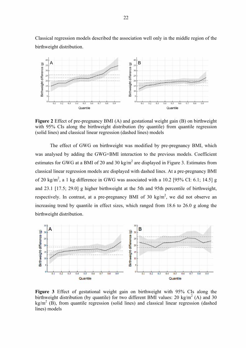
22

Classical regression models described the association well only in the middle region of the

birthweight distribution.

Figure 2 Effect of pre-pregnancy BMI (A) and gestational weight gain (B) on birthweight with 95% CIs along the birthweight distribution (by quantile) from quantile regression (solid lines) and classical linear regression (dashed lines) models

The effect of GWG on birthweight was modified by pre-pregnancy BMI, which

was analysed by adding the GWG×BMI interaction to the previous models. Coefficient

estimates for GWG at a BMI of 20 and 30 kg/m2 are displayed in Figure 3. Estimates from

classical linear regression models are displayed with dashed lines. At a pre-pregnancy BMI

of 20 kg/m2, a 1 kg difference in GWG was associated with a 10.2 [95% CI: 6.1; 14.5] g

and 23.1 [17.5; 29.0] g higher birthweight at the 5th and 95th percentile of birthweight,

respectively. In contrast, at a pre-pregnancy BMI of 30 kg/m2, we did not observe an

increasing trend by quantile in effect sizes, which ranged from 18.6 to 26.0 g along the

birthweight distribution.

Figure 3 Effect of gestational weight gain on birthweight with 95% CIs along the birthweight distribution (by quantile) for two different BMI values: 20 kg/m2 (A) and 30 kg/m2 (B), from quantile regression (solid lines) and classical linear regression (dashed lines) models

23

The effects of our hypothetical prevention strategies on birthweight related

pregnancy outcomes are summarised in Table 6. Calculations based on quantile regression

models showed that the relative decrease in the proportion of macrosomic infants (-15%)

was greater than the increase in low birthweight (+12%) after a hypothetical population-

based prevention strategy. Using coefficient estimates from classical regression models

resulted the opposite (-13% and +17%, respectively). The high-risk strategy slightly

increased the proportion of low birthweight infants, but the presence of macrosomia

decreased only by 6%.

Table 6 Efficacy of hypothetical prevention strategies (based on quantile regression coefficients) promoting a more modest gestational weight gain.

Prevention strategy Macrosomia %

Low birthweight %

SD

g Observed data 11.2 2.3 470 Population-based (-2 kg GWG) 9.6 2.5 465 High-risk (-3 kg GWG if BMI ≥ 25 kg/m2) 10.5 2.3 467

Values are based on non-parametric smooth kernel distributions.

5.2 Secular trends and age-related trajectories of risk factors Baseline characteristics of the Whitehall II cohort are shown in Table 7. Women

had generally lower employment grades and were more likely to be current smokers than

men. WC and HDL cholesterol differed the most between sexes.

5.2.1 Distributional trends (age group: 57-61 years) Risk factor percentiles (10th, 50th, 90th) for phases 3, 5, 7 and 9 and linear trends

from quantile regression models are displayed in Table 8. Smooth kernel distributions are

shown in Figure 4.

Changes in the BMI distribution of men were characterised by a right-shift of the

median and a fattening right tail. Increments were heterogeneous along the distribution and

were the largest at the 90th percentile (+2.8 kg/m2). For women the low BMI segment

remained unchanged, but the 90th percentile increased by 2 kg/m2 leading to a fat tail on

the right.

24

Table 7 Baseline characteristics of the Whitehall II cohort (1985-1988). Values are medians (Q1-Q3) or percentages.

Men (n=6,895) Women (n=3,413) Age (year) 43 (39-49) 45 (40-51) Whites (%) 91.5 84.2 Smoking (%)

Never 47.3 52.9 Ex 36.1 23.3 Current 15.8 23.3 Missing 0.8 0.5

Grade level (%) Administrative 38.4 11.2 Prof/Executive 52.3 39.1 Clerical/Support 9.3 49.7

BMI (kg/m2) 24.3 (22.6-26.2) 24.0 (21.9-26.7) WCa (cm) 88.9 (83.0-94.7) 76.5 (69.5-85.4) SBP (mmHg) 123 (115-133) 118 (109-130) DBP (mmHg) 77 (71-84) 75 (68-81) TC (mmol/l) 5.9 (5.2-6.7) 5.8 (5.1-6.6) HDL-C (mmol/l) 1.3 (1.1-1.6) 1.6 (1.4-2.0)

aWC measures are from phase 3 (1991-1994).

In contrast with BMI, WC increased along the entire distribution. The increment

was largest at the right end of the distribution (+8 cm at the 90th percentile) in both men

and women. The change in SBP was not consistent: it increased until phase 7 and then

dropped markedly at phase 9. Therefore the linear trend cannot be interpreted. In contrast

the entire DBP distribution shifted to the left by approximately 10 mmHg in both men and

women.

The linear trend was of similar magnitude along the entire TC distribution, which

led to a left-shift of the distribution with 1.5 mmol/l in both men and women. Changes in

HDL cholesterol were modest compared to TC, although all percentiles increased by 0.1-

0.2 mmol/l.

25

Table 8 Secular trends based on percentiles of risk factors in men and women.

Men Percentile Phase 3 n=911

Phase 5 n=903

Phase 7 n=1,222

Phase 9 n=1,391

Linear trenda (per year) β [95% CI]

BMI (kg/m2)

10th 21.9 22.2 22.4 21.9 0.004 [-0.014; 0.027] 50th 25.1 25.6 26.1 26.4 0.080 [0.065; 0.096]*** 90th 29.1 30.4 31.8 31.9 0.192 [0.145; 0.234]***

WC (cm)

10th 78.4 80.3 81.2 80.6 0.152 [0.100; 0.210]*** 50th 88.2 91.9 93.6 94.2 0.360 [0.318; 0.409]*** 90th 101.4 105.2 108.4 109.6 0.508 [0.433; 0.631]***

SBP (mmHg)

10th 107 106 109 107 0.000 [-0.086; 0.092] 50th 125 123 126 124 0.000 [-0.031; 0.083] 90th 145 148 150 143 -0.181 [-0.313; -0.030]*

DBP (mmHg)

10th 71 65 61 60 -0.654 [-0.714; -0.603]*** 50th 82 78 75 73 -0.594 [-0.653; -0.517]*** 90th 95 91 89 85 -0.577 [-0.650, -0.490]***

TC (mmol/l)

10th 5.3 4.8 4.5 4.0 -0.079 [-0.085; -0.074]*** 50th 6.7 5.9 5.7 5.2 -0.083 [-0.088; -0.077]*** 90th 8.1 7.3 7.0 6.6 -0.086 [-0.093; -0.079]***

HDL-C (mmol/l)

10th 0.9 1.0 1.0 1.0 0.005 [0.003; 0.008]*** 50th 1.3 1.3 1.4 1.4 0.008 [0.004; 0.010]*** 90th 1.8 1.9 1.9 2.0 0.011 [0.009; 0.013]***

Women Percentile Phase 3 n=520

Phase 5 n=383

Phase 7 n=492

Phase 9 n=514

Linear trenda (per year) β [95% CI]

BMI (kg/m2)

10th 21.3 21.2 21.2 21.1 -0.007 [-0.043; 0.021] 50th 26.0 25.8 25.8 26.1 0.000 [-0.023; 0.025] 90th 32.8 32.5 33.8 34.8 0.120 [0.063; 0.205]**

WC (cm)

10th 64.9 68.0 68.1 69.9 0.289 [0.190; 0.351]*** 50th 78.4 80.0 81.0 83.0 0.276 [0.173; 0.391]*** 90th 96.0 96.3 100.2 104.0 0.482 [0.354; 0.657]***

SBP (mmHg)

10th 104 103 104 99 -0.277 [-0.406; -0.091]** 50th 122 123 123 116 -0.350 [-0.516; -0.202]*** 90th 141 148 147 141 0.094 [-0.141; 0.278]

DBP (mmHg)

10th 66 64 60 56 -0.634 [-0.707; -0.524]*** 50th 78 75 72 69 -0.558 [-0.647; -0.491]*** 90th 90 89 88 84 -0.359 [-0.464; -0.201]***

TC (mmol/l)

10th 5.8 4.9 4.7 4.4 -0.084 [-0.093; -0.071]*** 50th 7.0 6.1 5.9 5.5 -0.084 [-0.093; -0.078]*** 90th 8.8 7.6 7.3 6.9 -0.115 [-0.122; -0.098]***

HDL-C (mmol/l)

10th 1.2 1.2 1.3 1.3 0.009 [0.007; 0.010]*** 50th 1.6 1.6 1.8 1.8 0.012 [0.010; 0.019]*** 90th 2.3 2.2 2.5 2.5 0.015 [0.011; 0.023]***

*p<0.05, **p<0.01, ***p<0.001 aLinear trends were assessed with quantile regression models.

26

Men

Women

Figure 4 Smooth kernel distributions of risk factors (probability density functions are displayed) in men and women (dotted line: phase 3, dashed line: phase 5, solid line: phase 7, thick line: phase 9)

27

Changes in the proportion of smokers and people on either lipid-lowering or

antihypertensive treatment are shown in Table 9. Fewer women smoked in the later phases,

while the number of smokers among men remained constant around 8%. Both lipid-

lowering and antihypertensive medication usage increased drastically. Between 2007 and

2009 approximately every fourth person was on treatment in the 57-61 age group.

Table 9 Secular trends of smoking habits, lipid-lowering and antihypertensive medication.

Phase 3 Phase 5 Phase 7 Phase 9 Men Current smoker 8.5 8.8 8.7 7.9 Lipid treatment 1.4 4.1 10.6 24.0 Anti-hyp. treatment 12.4 15.2 21.9 28.0 Women Current smoker 15.9 10.6 11.3 4.7 Lipid treatment 2.0 4.1 7.9 19.9 Anti-hyp. treatment 16.9 20.9 20.9 24.8

Values are percentages.

5.2.2 Age-related trajectories Age-related trajectories (unadjusted and adjusted for four different year of births)

of cardiometabolic risk factors - based on data from the entire Whitehall II cohort – are

displayed in Figure 5.

BMI and WC increased faster with age and were at higher levels at any given age

in younger birth cohorts than in older. The BMI difference between those born in 1933 and

1948 at age 60 was 1.3 [1.1; 1.5] kg/m2 and 0.5 [0.1; 0.9] kg/m2 in men and women,

respectively. The increasing trend of BMI was more marked in men, while women had

steeper BMI and WC trajectories in mid-life.

SBP increased faster between ages 40 and 75 in women than in men: 15.1 mmHg

versus 8.9 mmHg, which was a 12.9% and 7.2% relative increase, respectively. Younger

generations had generally lower mean SBP, except elderly men. The unadjusted mean

DBP trajectory had its peak around age 50 and then declined markedly. In the adjusted

models, younger generations’ trajectories started to decline earlier and had lower DBP at

any age.

28

Men

Women

Figure 5 Age-related trajectories of risk factors in men and women with adjustment for four different birth cohorts: 1933 (), 1938 (), 1943 (), 1948 () and unadjusted (---)

!

!!

! !

"

"

"" "

#

#

#

##

$

$

$

$$

40 50 60 70 8023

24

25

26

27

28

29

Age

Bodymassindex!kg"m

2#

! !!

!!

" ""

"

"

# ##

#

#

$$ $

$

$

40 50 60 70 80110

115

120

125

130

135

140

Age

Systolicbloodpressure!mmH

g" !!

!

!

!

"

" "

"

"

#

##

#

#$

$$

$

$

40 50 60 70 804.0

4.5

5.0

5.5

6.0

6.5

7.0

Age

Totalcholesterol!mmo

l"l#

!

!

!!

"

"

""

#

#

##

$

$

$$

40 50 60 70 80

70

75

80

85

90

95

100

Age

Waistcircumference!cm"

!!

!

!

!

""

"

"

"

#

# #

#

#

$

$ $

$

$

40 50 60 70 8060

65

70

75

80

85

Age

Diastolicbloodpressure!mmH

g"

! ! !!

!

" ""

"

"

# ##

#

#

$ $$

$

$

40 50 60 70 801.0

1.2

1.4

1.6

1.8

2.0

Age

HDLcholesterol!mm

ol"l#

!

!

!

!!

"

"

"

""

#

#

#

##

$

$

$

$$

40 50 60 70 8023

24

25

26

27

28

29

Age

Bodymassindex!kg"m

2#

!!

!

!

!

""

"

"

"

##

#

#

#

$$

$$

$

40 50 60 70 80110

115

120

125

130

135

140

Age

Systolicbloodpressure!mmH

g" !!

!

!

!

"

" "

"

"

#

##

#

#$

$$

$

$

40 50 60 70 804.0

4.5

5.0

5.5

6.0

6.5

7.0

Age

Totalcholesterol!mmo

l"l#

!

!

!!

"

"

""

#

#

##

$

$

$$

40 50 60 70 80

70

75

80

85

90

95

100

Age

Waistcircumference!cm" ! !

!

!

!

""

"

"

"

## #

#

#

$

$ $$

$

40 50 60 70 8060

65

70

75

80

85

Age

Diastolicbloodpressure!mmH

g"

! ! !!

!

" ""

"

"

# ##

#

#

$ $$

$

$

40 50 60 70 801.0

1.2

1.4

1.6

1.8

2.0

Age

HDLcholesterol!mm

ol"l#

29

The unadjusted TC trajectory of men increased up to age 47, peaking at 6.2 [6.2;

6.3] mmol/l. In women, the peak occurred slightly later at age 52, when the peak value was

6.3 [6.3; 6.4] mmol/l. At age 60, men born in 1948 had 1.1 [1.0; 1.2] mmol/l lower TC

level than men born in 1933, whereas for women the difference between these birth

cohorts was 1.2 [1.1; 1.3] mmol/l. Women had a higher mean HDL cholesterol level than

men from mid- to late-adulthood. We observed a modest increase with both age and

calendar year.

We found similar associations in our sensitivity analyses when fitting trajectories to

a subsample of participants who attended up to phase 9 (data not shown).

5.3 Diurnal variation of glucose measures OGTTs were performed between 08:00 and 15:00 (median 10:42, Q1-Q3:

9:50-11:36), whereas fasting duration ranged from 8 to 20 hours (median 13.4, Q1-Q3:

12.1-14.9). Time of day and fasting duration were moderately correlated (Pearson r = 0.6,

p<0.001).

The effect of time of day and fasting duration are summarised in Table 10. FPG

was inversely associated with both time of day and fasting duration. The mean difference

in FPG between measures at 08:00 and 15:00 was -0.46 [-0.50; -0.42] mmol/l in men

and -0.39 [-0.46; -0.31] mmol/l in women. The effect of fasting duration was markedly

attenuated after including both predictors in the model. Time of day and fasting duration

were positively associated with 2hPG. The mean difference between measures at 08:00 and

15:00 was 1.39 [1.25; 1.52] mmol/l in men and 1.19 [0.96; 1.42] mmol/l in women. Time

of day and fasting duration were independently associated with 2hPG even after the

inclusion of both variables in the model. HbA1c levels were neither associated with time of

day nor with fasting duration. Models with standardised outcome variables showed that the

relative impact of time of day and fasting duration on FPG and 2hPG were similar of

magnitude, but in the opposite direction (Figure 6).

30

Table 10 Estimated coefficients of time of day (TD) and fasting duration (FD) from age- and BMI-adjusted mixed-effects models for FPG, 2hPG and HbA1c with 95% CI.

Model variables Men Women FPG (mmol/l)

Only TD (h) -0.066 [-0.072; -0.059]*** -0.055 [-0.066; -0.044]*** Only FD (h) -0.033 [-0.037; -0.028]*** -0.024 [-0.031; -0.017]*** TD and FD

TD (h) -0.059 [-0.067; -0.050]*** -0.053 [-0.067; -0.039]*** FD (h) -0.007 [-0.012; -0.001]* -0.002 [-0.011; 0.007]

2hPG (mmol/l) Only TD (h) 0.198 [0.179; 0.217]*** 0.170 [0.137; 0.203]*** Only FD (h) 0.124 [0.111; 0.137]*** 0.103 [0.083; 0.124]*** TD and FD

TD (h) 0.128 [0.102; 0.154]*** 0.111 [0.068; 0.154]*** FD (h) 0.068 [0.051; 0.085]*** 0.058 [0.030; 0.085]***

HbA1c (%) Only TD (h) 0.000 [-0.007; 0.007] -0.006 [-0.018; 0.006] Only FD (h) 0.000 [-0.004; 0.005] -0.003 [-0.011; 0.005] TD and FD

TD (h) -0.001 [-0.009; 0.008] -0.005 [-0.021; 0.011] FD (h) 0.001 [-0.005; 0.006] -0.001 [-0.012; 0.009]

Figure 6 Standardised coefficient estimates of time of day (TD) and fasting duration (FD) for men (squares) and women (circles) with 95% confidence intervals. Displayed values are the differences caused by an our difference in TD and FD given in standard deviation of each outcome variable

31

The modifying effect of age and BMI on the diurnal variation (effect of time of

day) of glucose measure is summarised in Table 11. A higher BMI, but not increased age

was associated with larger diurnal variation in FPG. We observed the opposite relationship

for 2hPG: diurnal variation increased with ageing, but not with BMI.

Table 11 Diurnal variation of fasting plasma glucose by BMI and glucose tolerance (2hPG) by age (in mmol/l per 1 hour).

FPG BMI (kg/m2)

22 26 30 men -0.05 [-0.05; -0.04] -0.07 [-0.07; -0.06] -0.09 [-0.10; -0.08] women -0.04 [-0.05; -0.02] -0.05 [-0.07; -0.04] -0.07 [-0.09; -0.06]

2hPG Age (years)

45 60 75 men 0.15 [0.12; 0.18] 0.22 [0.19; 0.24] 0.28 [0.23; 0.33] women 0.12 [0.06; 0.17] 0.19 [0.16; 0.23] 0.27 [0.19; 0.35]

We modelled the hypothetical situation that all OGTTs started at 09:00 to

investigate the effect of our findings on the diagnosis of diabetes in a clinical setting. The

difference between the actual time of the OGTT and 09:00 was calculated (as a real

number in hours) and multiplied with the effect size of time of day from the mixed-effects

model. This value was added to the actual glucose measures. In this scenario, we found

that 15% of people with WHO-defined diabetes would have not received a diabetes

diagnosis. This was mainly driven by lower 2hPG values when measured hypothetically in

the morning. The number of people with “newly” diagnosed diabetes was not clinically

relevant.

32

6 DISCUSSION

6.1 Maternal obesity and gestational weight gain In this study, we investigated the association between BMI, GWG and birthweight

with quantile regression, a method that allows us to explore associations along the entire

distribution of an outcome. We discuss our results from a public health perspective.

6.1.1 Geoffrey Rose’s population approach

Geoffrey Rose’s population strategy still shapes public health practice and

preventive medicine [16–18]. His original idea poses that a smaller shift of the entire

distribution of exposure is likely to have a larger impact on risk reduction on a population

level, than a targeted approach focusing exclusively on high-risk individuals. This topic

still sparks debate in the literature of epidemiology [48–50]. Sophisticated statistical

models are necessary to evaluate the effect of hypothetical prevention strategies. Classical

regression models focusing on mean values cannot model distributional changes in an

outcome variable, because that would assume homogeneity in associations along the entire

outcome distribution. Our results showing varying effect sizes of BMI and GWG makes it

clear that the assumption of homogeneity does not hold for the BMI-birthweight and the

GWG-birthweight association. Use of classical regression may result in an underestimation

of the expected decrease in macrosomia and an overestimation of the increase in low

birthweight for a given population-wide reduction in GWG. Such results may lead to false

conclusions and even decisions on prevention policies. Our analyses suggest that quantile

regression is a more suitable tool to describe complex associations than classical regression

and calls for further methodological studies to describe and promote statistical models

beyond mean regression [51]. Using coefficients estimates from the quantile regression

models, we quantified the effect of two hypothetical prevention strategies. The population-

based approach (-2 kg GWG in all individuals) led to decreased dispersion (measured by

SD) of the birthweight distribution, which is favourable from a public health perspective.

This is the opposite of the common criticism against Rose’s population approach and

strengthens previous findings suggesting that it does not necessarily increase inequalities

[52, 53].

33

6.1.2 Targeted interventions

The population approach is usually set against a population-at-risk strategy that

targets only individuals at high risk. Such a strategy can be successful if accurate risk

assessment tools are available. Unfortunately, the prediction of fetal macrosomia is a

difficult task, even with modern diagnostic tools, because of complex associations of

environmental and genetic factors that determine fetal growth [54]. Our hypothetical high-

risk strategy targeted overweight and obese women, based on pre-pregnancy BMI, and

promoted a more intensive reduction of GWG (-3 kg) compared with the population

approach. Based on our calculation, the high-risk strategy underperformed the population

approach in the prevention of macrosomia. This was due to a relatively high proportion of

macrosomic infants, who were born to normal weight women. Our study population was

relatively lean: 21% of participants were overweight or obese. The increase in low

birthweight following the high-risk strategy was negligible, as expected. This approach of

prevention may be more effective in more obese populations.

6.1.3 Public health implications

A recent study investigated the effect of GDM, BMI and GWG on the birthweight

distribution using quantile regression [55]. The authors reported that individuals at higher

risk of having a macrosomic infant (in the right tail of the birthweight distribution) are

more vulnerable to changes in BMI and GWG. This finding is concerning if the obesity

epidemic continues and may have even more adverse effects on future generations. The

authors of the paper also called for further discussion how these results affect prevention

stategies targeting individuals at high risk. From the aspect of prevention, we think that the

heterogeneous effect of BMI and GWG on birthweight is in fact an opportunity to diminish

the right tail of the birthweight distribution without increasing the number of low

birthweight infants. Our results showed that a population approach promoting a more

modest GWG in all women may offer greater benefits on a population-level, than a high-

risk approach in a relatively lean population. This notion highlights the clinical and public

health importance of our findings, and the potentially detrimental consequences of using

statistical methods that do not model sufficiently the complexity of associations. Our

findings cannot be transferred in its original form to all risk factors, but show how quantile

regression may help to define risk reduction strategies in the presence of complex

associations between risk factors and outcomes.

34

6.1.4 Strengths and limitations

We analysed the effect of BMI and GWG on birthweight with quantile regression,

a method that gives a more complete picture of associations than classical regression

models. Although, quantile regression was developed more than 30 years ago, its

advantages have not been exploited in the field of epidemiology for a long time. Contrarily

to the only recent study investigating the effect of maternal obesity, we had information on

treatment received for diabetes during pregnancy, so this important factor, which could

have biased previous results, was accounted for in our analysis. Another strength of the

study was that BMI and GWG were kept as continuous variables to avoid loss of statistical

power.

The hypothetical prevention strategies were arbitrarily chosen and not optimised

for the study population. We considered only changes in GWG and not in pre-pregnancy

BMI, because in our opinion, although in many countries obese women wanting to be

pregnant are adviced to lose weight, women who are already pregnant are more motivated

to change their lifestyle habits, than the general population of women in childbearing age.

In the high-risk strategy, the targeted group was selected based on BMI using a threshold

value of 25 kg/m2. The efficacy of this strategy could be clearly improved with more

complex risk assessment tools, but our aim was mainly to illustrate how quantile

regression can help to estimate the effect of prevention strategies more accurately. The

relatively healthy and lean study population came from a rather affluent area of Budapest,

Hungary, so further investigation is necessary to replicate our results in other populations.

Pregnancy outcomes, other than birthweight, should be also analysed in the future.

6.2 Secular trends and age-related trajectories of risk factors We analysed secular trends and the natural progression of BMI, WC, SBP, DBP,

TC, HDL with ageing by assessing age-related trajectories based on a large longitudinal

dataset from the Whitehall II study (1985-2009). Distributional trends and age-related

changes are discussed and compared with other studies.

6.2.1 Obesity

Recent results show that the global obesity epidemic is leveling off in younger

generations, but increases are still observed among adult populations in Europe and Asia

[56]. This highlights the importance of revealing determinants of trends from an

35

epidemiological aspect. General obesity trends are usually described by reporting mean

BMI levels [4]. These results are easily interpreted, but give no information about the

shape of distributions. Another usual approach is to report the prevalence of overweight

and obesity [57–59]. This gives more, but still limited information on the higher segment

of the BMI distribution. Studies focusing on entire distributions showed an increased right-

skewness in the US [19, 20, 60–62], Canada [63], China and in low- and middle-income

countries [62, 64]. These studies were based on sequential cross-sectional analysis of

distributions in different population-samples and mainly based on descriptive percentile

statistics and to lesser extend on quantile regression [61]. This phenomenon that people

who are already obese are more affected by the obesity epidemic was previously called and

described as the “runaway weight gain train” [65]. The increasing BMI trend was more

marked in men. This finding strengthens previous evidence showing that obesity levels in

men are catching up with women [66–68]. One explanation might be a sex difference in

the attitude to weight management [69]. Women usually set lower weight goals than men,

who also have less attention on their ideal weight.

We observed that while BMI did not increase in leaner groups, they still developed

abdominal obesity indicated by a right-shift of the WC distribution’s lower segments. A

possible explanation is that people lose muscle mass and simultaneously accumulate

abdominal fat mass, because of more sedentary lifestyles. Our results are in line with

findings in low- and middle-income countries showing a 2-4 cm increase of WC at a given

level of BMI during a 18 years long period [70]. This notion is even more concerning in

light of previous evidence from the InterAct study showing a strong association between

abdominal obesity and glucose metabolism independently from general obesity [71]. A

recent review highlights the importance of the assessment of WC in addition to BMI,

because it gives independent information on obesity-related mortality [72]. Increasing

abdominal obesity is a public health concern that affect both sexes similarly and calls for

more attention on the development of prevention strategies.

Our longitudinal trajectory analyses showed that younger generations experience a

greater cumulative exposure to obesity. Participants born only 15 years later (in 1948

versus 1933), reached overweight 10 and 6 years earlier in their life-course in men and

women, respectively. We observed similar patterns in WC trajectories. The clinical

importance of these results are emphasised by recent findings of the CARDIA study [73].

36

The authors showed that a longer duration of general and abdominal obesity was linked to

coronary heart disease in midlife. The association was independent of the degree of

adiposity. This notion suggests that younger birth cohorts might be at a greater

cardiometabolic risk and that prevention of obesity is of major importance already at an

early age in the life-course. On the other hand, another study reported that reaching a

healthy weight is not too late in adulthood [74]. Their prospective analyses showed that

participants who were overweight or obese during childhood but not anymore in adulthood

had similar risk of type 2 diabetes, dyslipidemia and atherosclerosis, compared with those

who were never overweight or obese.

Our analyses clearly showed that cohort effect should not be ignored when

assessing age-related trajectories. While the oldest participants of the Whitehall II cohort

grew up in the austerity of the 1930s, younger generations were born in the period of post-

war reconstruction, increasing welfare and food security. Recent results show that such

effects still exists, as the height and weight of 6-year-old children increased in the last 30

years and obesity prevalence continues to rise in less affluent populations [75]. Age-related

changes cannot be analysed adequately based on cross-sectional data. A previous study

reported that age-related increases in BMI might be underestimated in such analyses [76].

In addition, we argue that longitudinal analyses give biased estimates when cohort effects

are ignored. Therefore we modelled cohort effects by adding year of birth (time-invariant

variable) and its interaction with age to the models. The interaction term is responsible for

the different curve characteristics (e.g. curvature and slope at a given age). Keeping age

and year of birth as continuous variables is advisable to retain statistical power.

6.2.2 Blood pressure Contrary to our observations in obesity measures, distributional trends in SBP were

not consistent in one direction between phases. A marked decline was observed only

between phase 7 and 9, especially in women. We cannot fully attribute this decline to a

wider use of antihypertensive medication, because that increased already between earlier

phases. In contrast, both our sequential cross-sectional and longitudinal analyses confirm a

marked decline in DBP. The drop was similar along the entire distribution, which resulted

a left-shift of the distribution. Regarding the age-related blood pressure trajectories, our

results are in line with current understanding that SBP rises from mid to late adulthood

(more rapidly among women), while DBP peaks around the age of 50 years and then starts

37

to decline, because of increasing aortic and small vessel stiffness [45, 77]. Compared to

previous studies, our analyses accounted for secular trends and cohort effects that made it

possible to observe different trajectory characteristics between birth cohorts. In addition to

generally lower DBP levels, we also found that the decline started at a lower age in

younger birth cohorts. As DBP is inversely associated with the risk of coronary heart

disease after age 60, this notion imposes additional risk on younger birth cohorts [78]. The

decreasing trends in SBP and especially in DBP have to be interpreted with caution. As

DBP decreases with age while SBP increases, a widening gap develops between SBP and

DBP that leads to an increasing pulse pressure, which is an independent determinant of the

coronary heart disease [79]. In addition to an increase with ageing, pulse pressure has also

increased with calendar year, leading to an additional risk of CVD due to a combined

cohort and period effect.

6.2.3 Cholesterol

In contrast to previous studies, which reported trends based on mean levels, we

analysed secular trends along the entire TC distribution. Our results showed a marked left-

shift of the entire distribution, which extends previous knowledge on decreasing trends [6,

80, 81]. Although the observed decline may be partially due to the wider use of statins,

especially in elderly, this cannot be the only cause, as values decreased in the left tail of the

distribution too. This finding is in line with previous reports from developed countries

emphasising the importance of positive changes in dietary patterns [46, 82]. They also

argue that the marked decline started already before statins were introduced and further

regulatory interventions are necessary to promote the use of healthier fats. Our analyses

showed that the age-related trajectories of younger cohorts started to decline at younger

ages in the life-course. It is likely because of decreasing thresholds above which lipid-

lowering treatment is prescribed. The effect of secular trends and cohort effects were so

large during the last three decades that an unadjusted TC trajectory clearly underestimates

true trajectories in late adulthood. This effect makes it a challenging task to isolate the

effect of ageing from trends. Trends in HDL cholesterol are rarely investigated. Both of

our models suggest favourable changes in HDL cholesterol levels in the last three decades.

Although changes in HDL cholesterol were modest compared to TC.

38


When analysing secular trends, we did not only report mean levels of risk factors,

but considered entire distribution characteristics. Quantile regression is a suitable tool for

such analyses. Age-related trajectories were assessed based on a long period of observation

(25 years) with up to five repeated measurements per person. Secular trends, cohort effects

and ageing were considered simultaneously in our analyses.

Handling missing data and attrition are important tasks when analysing longitudinal

data. When the pattern of missingness is MAR, mixed-effects models give valid estimates

for the age-related trajectories. To handle the case of MNAR, we conducted sensitivity

analyses on a subgroup of individuals who participated up to phase 9. These analyses

replicated our main findings, indicating that it is unlikely that loss to follow-up biased our

age-trajectory estimates. When the follow-up period is long, standardisation of

measurements is crucial and cannot be ignored. All laboratories participated in the

National External Quality Assurance Scheme for TC and HDL cholesterol. Regarding

blood pressure measures, it is unlikely that decreasing trends were due to changes in

measurement device, because AOD used in the last two phases, produces slightly higher

values than MRZ [83]. Our results were based on an occupational cohort study. Such

cohorts are usually healthier than the general population. Previous studies from the

Whitehall II study showed lower mortality rates [84], lower SBP trajectories, but similar

BMI trajectories compared with population-based cohorts [45]. Another limitation of our

sequential cross-sectional analysis, was that we could analyse only the 57-61 age group.

Further research is necessary to confirm our results on a population level.

6.3 Diurnal variation of glucose measures 6.3.1 Diabetes diagnosis

Diurnal variation of glucose tolerance has not received much attention in the past

decades, even though the definition of diabetes has been based on fasting and/or 2-hour

post-OGTT values since 1965. After the recent introduction of HbA1c as an additional

diagnostic criterion, analyses investigating the overlap between HbA1c and OGTT based

diabetes diagnosis have implicitly assumed the OGTT to be a type of gold standard.

Previous studies also showed a significant intra-individual variation of glucose measures.

This result had important clinical implications: approximately 20% of patients who

39

received a diagnosis based on an OGTT, would not have a diagnosis when retested [85].

Our analysis, based on a large sample of repeated measures in a well characterised cohort,

shows that even a few hours difference in fasting duration or sampling time can affect

whether or not somebody is diagnosed as having diabetes based on an OGTT.

6.3.2 Fasting glucose

The observed decline in FPG levels during the day is in line with previous findings,

which also showed clinically relevant differences between morning and early afternoon

FPG measures [28]. Our findings support the notion that standardisation of fasting duration

and time of day is an important point in the protocols of epidemiological studies [29].

Glucose measures even from fasting subjects are not necessarily unbiased, so adjustment

for timing factors is advisable if data are available. These results indicate that timing

should not be ignored when diagnosing diabetes, or comparing individual glucose levels

longitudinally in clinical practice. Our results are also consistent with previous findings on

the modest role of fasting duration in addition to time of day [30]. We agree with the

authors conclusions that more effort on the standardisation or assessment of other factors,

like diet and physical activity, is necessary.

6.3.3 Glucose tolerance (2hPG) Our results are consistent with previous evidence, indicating higher 2hPG levels in

the afternoon than in the morning [25–27]. We also confirmed the notion that diurnal

variation in glucose tolerance increases with age. However, we found no clear evidence to

suggest that obesity would reduce diurnal variation in 2hPG [26]. A previous review

reported that there is no evidence for an effect of fasting duration in addition to time of day

[86]. In contrast, fasting duration improved our models for 2hPG even if time of day was

accounted for. This difference might be because of the lack of statistical power or different

protocols regarding fasting duration in previous studies. Although the studies are not

directly comparable, our results support the recent finding of an underestimation of glucose

tolerance among pregnant women who had an afternoon rather than a morning 1-hour,

50 g, non-fasting glucose challenge test, as compared to a confirmatory morning 3-hour,

100 g fasting OGTT performed on a separate day [87].

6.3.4 HbA1c HbA1c reflects blood glucose concentrations retrospectively in the previous 2-3

months. As a result of a WHO expert consultation in 2009, it was recently accepted as a

40

new diagnostic tool for diabetes. A recent study reported that HbA1c is not only useful to

predict future diagnosis of diabetes, but had an even stronger association with the risk of

CVD and death from all cause mortality than FPG [88]. Similarly stronger associations

were found between HbA1c and ischaemic heart disease in a large Danish population [89].

In addition to these findings, one of the most important features of an HbA1c test remains

the independence of results from time of day and fasting duration. We confirmed this

notion in a large occupational cohort study.


The key strength of our study was that we did not categorise time of day and

fasting duration. This was possible because of the detailed assessment of variables.

Another strength of our study was, that we analysed all three measures parallel in the same

population. However, the relatively low proportion of women in the study resulted in wider

confidence intervals for their coefficient estimates. The longitudinal structure of the dataset

was neither an advantage nor a disadvantage, because it was handled according to common

practice by adding random effects to the models and adjusting them for study phase. Our

analyses were based on data from an occupational cohort, that is known to be relatively

healthier than the general population. Further research is needed to examine the

generalisability of our findings to other populations, ethnic groups and pregnant women.

41

7 SUMMARY AND CONCLUSIONS

Maternal obesity and GWG are targets for prevention of adverse pregnancy

outcomes related to birthweight. Using quantile regression, we found that GWG was

positively associated with infant birthweight, however in leaner women its effect was

heterogeneous along the distribution of birthweight and increased towards higher

percentiles. Classical regression models cannot reveal such differences and give a rather

incomplete picture of associations. We also evaluated the effect of hypothetical prevention

strategies on the birthweight distribution. We concluded that a population-wide lowering

of GWG would not lead to a uniform left-shift of the birthweight distribution, but that the

right tail would be more affected and the total variance would decrease. Our findings

support the promotion of strategies to lower GWG on a population-level. These results

indirectly imply that current GWG guidelines might be too permissive. We also conclude

that quantile regression is a useful tool for epidemiologists and public health practitioners

to investigate complex, distributional associations of risk factors and outcomes.

The past 25 years brought marked changes in cardiometabolic risk factors. Younger

generations were more obese, than their older peers at any given age. Contrarily, we

observed a more favourable lipid profile (i.e. lower TC levels and higher HDL cholesterol

levels) in younger cohorts. Furthermore, the observed secular trends affected the shape of

risk factor distributions. Whereas the increase in obesity led to more right-skewness, the

decreases in TC and interestingly in DBP were characterised by a left-shift of the entire

distributions. These results show that the last three decades brought strong and

heterogeneous secular trends in obesity, blood pressure and lipid levels. Decreasing CVD

mortality in the UK suggest that the negative trends in obesity are counterbalanced by

favourable changes in other risk factors. The disparity of these trends indicate that the

relative importance of these risk factors is likely to change over time. This observation has

potential implications for the way we assess global CVD risk based on risk scores,

highlighting the need to reassess the calibration of component weights on a regular basis.

Our findings also suggest that more detailed models of risk factor progression may be

needed to help track the development not only of mean levels but also changing risk factor

distributions in the population. Secular trends caused by period and cohort effects should

be considered in longitudinal analyses of age-related risk factor trajectories to avoid biased

estimates.

42

The diagnosis of diabetes is based on blood glucose levels, therefore the

investigation of factors influencing glucose levels on a population level is an important

task from an epidemiological perspective. Based on a large sample, we showed that time of

blood sampling and duration of fasting prior to blood sampling affect FPG and 2hPG

levels considerably. As expected, neither of these factors affected HbA1c. Furthermore we

showed how age and BMI affect the diurnal variation of glucose tolerance and fasting

glucose measures. These results highlight the importance of standardising the diagnostic

OGTT regarding time of day and fasting duration that is often overlooked in clinical

practice and in epidemiological investigations. FPG and 2hPG measures vary by different

fasting duration periods even after 8 hours of fasting, independently of time of blood

sampling. This finding suggests that the current WHO recommendation may not be strict

enough regarding time of blood sampling and fasting duration and adjustment for these

factors is necessary in clinical practice and epidemiological studies.

Epidemiology provides the scientific basis for public health practice by exploring

the “occurrence and distribution of health-related states or events in specified populations,

including the study of the determinants influencing such states, and the application of this

knowledge to control the health problems” [90]. Our studies demonstrated that the use of

appropriate statistical methods is crucial when exploring the relative importance of risk

factors and their associations with health-related outcomes, identifying subgroups at risk

and evaluating the effectiveness of prevention strategies. With the knowledge gathered in

developed countries, where CVD incidence already seems to be declining, a huge burden

of disease can hopefully be prevented in developing countries which are going through

similar economical and societal changes to those that were already seen in high-income

regions. Adequate control of modifiable risk factors is a key tool to achieve this goal.

43

Novelties and key messages

Maternal obesity and gestational weight gain

• We demonstrated the rarely exploited potential of quantile regression in public

health and preventive medicine.

• The association between gestational weight gain and birthweight was altered by

BMI and was heterogeneous in leaner women.

• Based on a statistical model, we found that a population-based intervention

promoting a more modest gestational weight gain might offer more favourable

changes in the birthweight distribution, than a high-risk approach.

Secular trends and age-related trajectories of risk factors

• Trends of cardiometabolic risk factors were described using sophisticated

statistical methods focusing on entire distribution characteristics and not only on

mean levels.

• The obesity epidemic affected those already overweight and obese, which led to

increasing dispersion and right-skewness of distributions.

• The marked drop in diastolic blood pressure has to be interpreted with caution,

because of its negative effects in elderly and the increasing pulse pressure.

• Secular trends were strong and heterogeneous in the last decades and therefore

should be taken into account when analysing age-related trajectories to avoid

biased estimates caused by large differences between successive birth cohorts.

Diurnal variation of glucose measures

• We investigated the combined effect of time of day and fasting duration on all

three glucose measures, based on a large sample.

• We gave estimates for the magnitude of diurnal variation by keeping time of day

and fasting duration as continuous variables.

• Time of blood sampling and fasting duration have clinically relevant effects on

glucose measures even if WHO recommendations are followed.

44

8 ACKNOWLEDGEMENTS

During the last few years I have received support and encouragement from a great

number of individuals.

First of all, I would like to thank Daniel R. Witte, my external supervisor for his

invaluable support and guidance during my Ph.D. studies. I feel very lucky that he

introduced me to the field of epidemiology and that we are working together. I have learnt

a lot during our conversations and from his insightful comments on our papers,

presentations and the present thesis. Special thanks go to him also for introducing me to

the European Diabetes Epidemiology Group, we had some memorable meetings in the last

three years.

I would like to express my gratitude to my supervisors in Szeged: János Karsai and

Tibor Nyári for their motivation, support and patience. János played an important role in

that I ended up pursuing a career in life sciences as an applied mathematician. He gave me

the first real-life problems to inspire me when I was still studying mathematics and invited

me to the Department of Medical Physics and Informatics, my current workplace. Tibor

helped me a lot to get more experience in biostatistics and epidemiology, and was always

extremely encouraging with me.

I would like to express my gratitude to Ferenc Bari, head of the Department of

Medical Physics and Informatics for his support and advice on my career.

I would like to give special thanks to Grant Fuller and Balázs Boros, my former

colleagues in London, for their motivation and support. It was a fantastic opportunity for

me to work with them, which really formed my professional attitude.

I would also like to thank some of my co-authors: Ádám Tabák (Semmelweis

University), Dorte Vistisen, Kristine Færch (Steno Diabetes Center), Eric J. Brunner and

Mika Kivimäki (UCL) for their help and useful comments on our papers.

I am also grateful to my colleagues at my home institute, especially to my fellow

Ph.D. students. It was a pleasure to have some fun with them during lunchtimes.

Last but not least, I also wish to thank my family, especially my parents and my

wife for their constant support, encouragement and patience.

45

9 REFERENCES

1. World Health Organization. Global status report on noncommunicable diseases 2010. Available at: http://www.who.int/nmh/publications/ncd_report2010/en/ (Accessed: 3 April 2014)

2. Zhang P, Zhang X, Brown J, et al. Global healthcare expenditure on diabetes for 2010 and 2030. Diabetes Res Clin Pract 2010;87:293–301.

3. Mahmood SS, Levy D, Vasan RS, Wang TJ. The Framingham Heart Study and the epidemiology of cardiovascular disease: a historical perspective. Lancet 2014;383:999–1008.

4. Finucane MM, Stevens GA, Cowan MJ, et al. National, regional, and global trends in body-mass index since 1980: systematic analysis of health examination surveys and epidemiological studies with 960 country-years and 9·1 million participants. Lancet 2011;377:557-67.

5. Danaei G, Finucane MM, Lin JK, et al. National, regional, and global trends in systolic blood pressure since 1980: systematic analysis of health examination surveys and epidemiological studies with 786 country-years and 5·4 million participants. Lancet 2011;377:568-77.

6. Farzadfar F, Finucane MM, Danaei G, et al. National, regional, and global trends in serum total cholesterol since 1980: systematic analysis of health examination surveys and epidemiological studies with 321 country-years and 3·0 million participants. Lancet 2011;377:578-86.

7. Danaei G, Finucane MM, Lu Y, et al. National, regional, and global trends in fasting plasma glucose and diabetes prevalence since 1980: systematic analysis of health examination surveys and epidemiological studies with 370 country-years and 2·7 million participants. Lancet 2011;378:31–40.

8. Anand SS, Yusuf S. Stemming the global tsunami of cardiovascular disease. Lancet 2011;377:529–32.

9. Heslehurst N, Rankin J, Wilkinson JR, et al. A nationally representative study of maternal obesity in England , UK  : trends in incidence and demographic inequalities in 619 323 births, 1989-2007. Int J Obes 2010;34:420–8.

10. Han Z, Mulla S, Beyene J, et al. Maternal underweight and the risk of preterm birth and low birth weight: a systematic review and meta-analyses. Int J Epidemiol 2011;40:65–101.

11. Mcdonald SD, Han Z, Mulla S, et al. Overweight and obesity in mothers and risk of preterm birth and low birth weight infants: systematic review and meta-analyses. BMJ 2010;341:c3428.

12. Oza‐Frank R, Keim SA. Should Obese Women Gain Less Weight in Pregnancy Than Recommended? Birth 2013;40:107–114.

13. IOM (Institute of Medicine) and NRC (National Research Council). Weight gain during pregnancy: reexamining the guidelines. Washington D.C.: The National Academies Press; 2009.

46

14. Nohr EA, Vaeth M, Baker JL, et al. Combined associations of prepregnancy body mass index and gestational weight gain with the outcome of pregnancy. Am J Clin Nutr 2008;87:1750–9.

15. Keyes KM, Utz RL, Robinson W, et al. What is a cohort effect? Comparison of three statistical methods for modeling cohort effects in obesity prevalence in the United States, 1971-2006. Soc Sci Med 2010;70:1100–8.

16. Rose G. Strategy of prevention: lessons from cardiovascular disease. BMJ 1981;282:1847–51.

17. Rose G. Sick individuals and sick populations. Int J Epidemiol 1985;14:32–8.

18. Doyle YG, Furey A, Flowers J. Sick individuals and sick populations: 20 years later. J Epidemiol Community Health. 2006;60:396–8.

19. Flegal KM, Troiano RP. Changes in the distribution of body mass index of adults and children in the US population. Int J Obes 2000;24:807–18.

20. Penman AD, Johnson WD. The changing shape of the body mass index distribution curve in the population: implications for public health policy to reduce the prevalence of adult obesity. Prev Chronic Dis 2006; 3:A74.

21. Long GH, Simmons RK, Norberg M, et al. Temporal shifts in cardiovascular risk factor distribution. Am J Prev Med 2014;46:112–21.

22. World Health Organization and International Diabetes Federation. Definition and diagnosis of diabetes mellitus and intermediate hyperglycemia (2006). Available at: http://www.who.int/diabetes/publications/diagnosis_diabetes2006/en/ (Accessed: 3 April 2014)

23. World Health Organization. Use of glycated haemoglobin (HbA1c) in the diagnosis of diabetes mellitus (2011). Available at: http://www.who.int/diabetes/publications/diagnosis_diabetes2011/en/ (Accessed: 3 April 2014)

24. Goldstein DE, Little RR, Lorenz RA, et al. Tests of glycemia in diabetes. Diabetes Care 2004;27:1761–73.

25. Jarrett RJ, Keen H. Diurnal variation of oral glucose tolerance: a possible pointer to the evolution of diabetes mellitus. BMJ 1969;2:341–4.

26. Zimmet PZ, Wall JR, Rome R, et al. Diurnal variation in glucose tolerance: associated changes in plasma insulin, growth hormone, and non-esterified fatty acids. BMJ 1974;1:485–8.

27. Mayer KH, Stamler J, Dyer A, et al. Epidemiologic findings on the relationship of time of day and time since last meal to glucose tolerance. Diabetes 1976;25:936–43.

28. Troisi RJ, Cowie CC, Harris MI Diurnal variation in fasting plasma glucose: implications for diagnosis of diabetes in patients examined in the afternoon. JAMA 2000;284:3157–9.

29. Emberson JR, Whincup PH, Walker M, et al. Biochemical measures in a population-based study  : effect of fasting duration and time of day. Ann Clin Biochem 2002;39:493–501.

47

30. Moebus S, Göres L, Lösch C, et al. Impact of time since last caloric intake on blood glucose levels. Eur J Epidemiol 2011;26:719–28.

31. World Health Organization. Definition, diagnosis and classification of diabetes mellitus and its complications (1999). Available at: http://whqlibdoc.who.int/hq/1999/who_ncd_ncs_99.2.pdf (Accessed: 3 April 2014)

32. Mosteller F, Tukey JW. Data analysis and regression: a second course in statistics. Reading, MA: Addison-Wesley; 1977.

33. Abrevaya J. The effects of demographics and maternal behavior on the distribution of birth outcomes. Empir Econ. 2001;26:247–57.

34. Koenker R, Bassett G, Jan N. Regression Quantiles. Econometrica 1978;46:33–50.

35. Koenker R, Hallock KF. Quantile Regression. J Econ Perspect 2001;15:143–56. 36. Koenker R. quantreg: Quantile regression. R package version 4.97.

Available at: http://www.inside-r.org/packages/cran/quantreg (Accessed: 3 April 2014)

37. Singer J, Willett J. Applied longitudinal data analysis: modeling change and event occurence. New York, NY: Oxford University Press; 2003.

38. Gałecki A, Burzykowski T. Linear mixed-effects models using R. New York, NY: Springer; 2013.

39. Bates DM. lme4: Mixed-effects modeling with R. Available at: http://lme4.r-forge.r-project.org/lMMwR/lrgprt.pdf (Accessed: 3 April 2014)

40. Kerényi Z, Tamás G, Kivimaki M, et al. Maternal glycemia and risk of large-for-gestational-age babies in a population-based screening. Diabetes Care 2009;32:2200–5.

41. Marmot M, Brunner E. Cohort Profile: the Whitehall II study. Int J Epidemiol 2005;34:251–6.

42. Tabák AG, Jokela M, Akbaraly TN, et al. Trajectories of glycaemia, insulin sensitivity, and insulin secretion before diagnosis of type 2 diabetes: an analysis from the Whitehall II study. Lancet 2009;373:2215–21.

43. Stringhini A, Tabák AG, Akbaraly TN, et al. Contribution of modifiable risk factors to social inequalities in type 2 diabetes: prospective Whitehall II cohort study. BMJ 2012;345:e5452.

44. Færch K, Witte DR, Tabák AG, et al. Trajectories of cardiometabolic risk factors before diagnosis of three subtypes of type 2 diabetes: a post-hoc analysis of the longitudinal Whitehall II cohort study. Lancet Diabetes Endocrinol 2013;1:43–51.

45. Wills AK, Lawlor DA, Matthews FE, et al. Life course trajectories of systolic blood pressure using longitudinal data from eight UK cohorts. PLoS Med 2011;8:e1000440.

48

46. Bouillon K, Singh-Manoux A, Jokela M, et al. Decline in low-density lipoprotein cholesterol concentration: lipid-lowering drugs, diet, or physical activity? Evidence from the Whitehall II study. Heart 2011;97:923–30.

47. Faerch K, Borch-Johnsen K, Vaag a, et al. Sex differences in glucose levels: a consequence of physiology or methodological convenience? The Inter99 study. Diabetologia 2010;53:858–65.

48. Frohlich KL, Potvin L. Transcending the known in public health practice: the inequality paradox: the population approach and vulnerable populations. Am J Public Health 2008;98:216–21.

49. Zulman DM, Vijan S, Omenn GS, et al. The relative merits of population-based and targeted prevention strategies. Milbank Q 2008;86:557–80.

50. Ahern J, Jones MR, Bakshis E, et al. Revisiting rose: comparing the benefits and costs of population-wide and targeted interventions. Milbank Q 2008;86:581–600.

51. Kneib T. Beyond mean regression. Stat Model 2013;13:275–303. 52. Liu SY, Kawachi I, Glymour MM. Education and inequalities in risk scores for

coronary heart disease and body mass index: evidence for a population strategy. Epidemiology 2012;23:657–64.

53. McLaren L, McIntyre L, Kirkpatrick S. Rose’s population strategy of prevention need not increase social inequalities in health. Int J Epidemiol 2010;39:372–7.

54. Walsh JM, McAuliffe FM. Prediction and prevention of the macrosomic fetus. Eur J Obstet Gynecol Reprod Biol 2012;162:125–30.

55. Ellerbe CN, Gebregziabher M, Korte JE, et al. Quantifying the impact of gestational diabetes mellitus, maternal weight and race on birthweight via quantile regression. PLoS One 2013;8:e65017.

56. Rokholm B, Baker JL, Sørensen TIA. The levelling off of the obesity epidemic since the year 1999 - a review of evidence and perspectives. Obes Rev 2010;11:835–46.

57. Flegal KM, Carroll MD, Ogden CL, et al. Prevalence and trends in obesity among US adults, 1999-2000. JAMA 2002;288:1723–7.

58. Flegal KM, Carroll MD, Ogden CL, et al. Prevalence and trends in obesity among US adults, 1999-2008. JAMA 2010;303:235–41.

59. Flegal KM, Carroll MD, Kit BK, Ogden CL. Prevalence of obesity and trends in the distribution of body mass index among US adults, 1999-2010. JAMA 2012;307:491–7.

60. Gordon-Larsen P, Adair LS, Nelson MC, et al. Five-year obesity incidence in the transition period between adolescence and adulthood: the National Longitudinal Study of Adolescent Health. Am J Clin Nutr 2004;80:569–75.

61. Bottai M, Frongillo EA, Sui X, et al. Use of quantile regression to investigate the longitudinal association between physical activity and body mass index. Obesity 2013;doi:10.1002/oby.20618.

49

62. Razak F, Corsi DJ, Subramanian SV. Change in the body mass index distribution for women: analysis of surveys from 37 low- and middle-income countries. PLoS Med 2013;10:e1001367.

63. Katzmarzyk PT. The Canadian obesity epidemic: an historical perspective. Obes Res 2002;10:666–74.

64. Xi B, Liang Y, He T, et al. Secular trends in the prevalence of general and abdominal obesity among Chinese adults, 1993-2009. Obes Rev 2012;13:287–96.

65. Swinburn B, Egger G. The runaway weight gain train: too many accelerators, not enough brakes. BMJ 2004;329:736–9.

66. Cabrera C, Wilhelmson K, Allebeck P, Wedel H, Steen B, Lissner L. Cohort differences in obesity-related health indicators among 70-year olds with special reference to gender and education. Eur J Epidemiol 2003;18:883–90.

67. Eiben G, Dey DK, Rothenberg E, et al. Obesity in 70-year-old Swedes: secular changes over 30 years. Int J Obes 2005;29:810–7.

68. Lahti-Koski M, Jousilahti P, Pietinen P. Secular trends in body mass index by birth cohort in eastern Finland from 1972 to 1997. Int J Obes 2001;25:727–34.

69. Crawford D, Campbell K. Lay definitions of ideal weight and overweight. Int J Obes Relat Metab Disord 1999;23:738–45.

70. Popkin BM, Slining MM. New dynamics in global obesity facing low- and middle-income countries. Obes Rev 2013;doi:10.1111/obr.12102.

71. The InterAct Consortium. Long-term risk of incident type 2 diabetes and measures of overall and regional obesity: the EPIC-InterAct case-cohort study. PLoS Med 2012;9:e1001230.

72. Carmienke S, Freitag MH, Pischon T, et al. General and abdominal obesity parameters and their combination in relation to mortality: a systematic review and meta-regression analysis. Eur J Clin Nutr 2013;67:573–85.

73. Reis JP, Loria CM, Lewis CE, et al. Association Between Duration of Overall and Abdominal Obesity Beginning in Young Adulthood and Coronary Artery Calcification in Middle Age. JAMA 2013;310:280–8.

74. Juonala M, Magnussen CG, Berenson GS, et al. Childhood adiposity, adult adiposity, and cardiovascular risk factors. N Engl J Med 2011;365:1876–85.

75. Smith SM, Craig LCA, Raja AE, McNeill G, Turner SW. Growing up before growing out: secular trends in height, weight and obesity in 5--6-year-old children born between 1970 and 2006. Arch Dis Child 2013;98:269–73.

76. Nooyens ACJ, Visscher TLS, Verschuren WMM, et al. Age, period and cohort effects on body weight and body mass index in adults: The Doetinchem Cohort Study. Public Health Nutr 2009;12:862–70.

77. Cheng S, Xanthakis V, Sullivan LM, Vasan RS. Blood pressure tracking over the adult life course: patterns and correlates in the Framingham heart study. Hypertension 2012;60:1393–9.

50

78. Franklin SS, Larson MG, Khan SA, et al. Does the relation of blood pressure to coronary heart disease risk change with aging?  : The Framingham Heart Study. Circulation 2001;103:1245–9.

79. Assmann G, Cullen P, Evers T, Petzinna D, Schulte H. Importance of arterial pulse pressure as a predictor of coronary heart disease risk in PROCAM. Eur Heart J 2005;26:2120–6.

80. Arnett DK, Jacobs DR, Luepker RV, Blackburn H, Armstrong C, Claas SA. Twenty-year trends in serum cholesterol, hypercholesterolemia, and cholesterol medication use: the Minnesota Heart Survey, 1980-1982 to 2000-2002. Circulation 2005;112:3884–91.

81. Scholes S, Bajekal M, Love H, et al. Persistent socioeconomic inequalities in cardiovascular risk factors in England over 1994-2008: a time-trend analysis of repeated cross-sectional data. BMC Public Health 2012;12:129.

82. Capewell S, Ford ES. Why have total cholesterol levels declined in most developed countries? BMC Public Health 2011;11:641.

83. Stang A, Moebus S, Möhlenkamp S, et al. Algorithms for converting random-zero to automated oscillometric blood pressure values, and vice versa. Am J Epidemiol 2006;164:85–94.

84. Singh-Manoux A, Guéguen A, Ferrie J, et al. Gender differences in the association between morbidity and mortality among middle-aged men and women. Am J Public Health 2008;98:2251–7.

85. Selvin E, Crainiceanu CM, Brancati FL, et al. Short-term variability in measures of glycemia and implications for the classification of diabetes. Arch Intern Med 2007;167:1545–51.

86. Van Cauter E, Polonsky KS, Scheen AJ. Roles of circadian rhythmicity and sleep in human glucose regulation. Endocr Rev 1997;18:716–38.

87. Goldberg RJ, Ye C, Sermer M, et al. Circadian variation in the response to the glucose challenge test in pregnancy: implications for screening for gestational diabetes mellitus. Diabetes Care 2012;35:1578–84.

88. Selvin E, Steffes M, Zhu H, et al. Glycated hemoglobin, diabetes, and cardiovascular risk in nondiabetic adults. N Engl J Med 2010;362:800–11.

89. Borg R, Vistisen D, Witte DR, et al. Comparing risk profiles of individuals diagnosed with diabetes by OGTT and HbA1c The Danish Inter99 study. Diabet Med 2010;27:906–10.

90. International Epidemiological Association. Dictionary of Epidemiology. New York, NY: Oxford University Press; 2008.

Documents

EPIDEMIOLOGICAL ASPECTS OF CARDIOMETABOLIC RISK