Environmental Considerations for Xenon Electric Propulsion

The 30

th International Electric Propulsion Conference, Florence, Italy

September 17-20, 2007

1

Environmental Considerations for Xenon Electric

Propulsion

IEPC-2007-257

Presented at the 30th International Electric Propulsion Conference, Florence, Italy


Mark W. Crofton* and Toby D. Hain†

The Aerospace Corporation, Los Angeles, CA, 90009, U.S.A.

Abstract: In the present study, the focus is on potential environmental effects associated with electric

thrusters that use xenon propellant. The study is broad in scope, providing background on electric

propulsion systems, structure of the atmosphere, xenon production and applications, xenon chemistry, etc.

Few measurement data exist concerning the atmospheric distribution of xenon, therefore this distribution has

been calculated. Although the plume concentration near the thruster is much greater than natural

abundance levels, the increase in atmospheric concentration due to its release from an ion thruster is shown

to be small at all altitudes, even for volumes of modest size. Eroded species emitted from xenon electric

thrusters, after a modest amount of atmospheric transport and mixing, similarly are found to be relatively

insignificant in comparison to natural sources. In the worst case - rapid release of the entire contents of the

propellant tank, after a short diffusion period measured in hours the natural abundance will dominate.

Neutral atoms released from the thrusters can be ionized via several mechanisms. These rates are considered

in the paper, and it is concluded that at operational altitudes xenon will exist predominantly in the ionized

form. Xenon is a noble gas, but due to its position in the periodic table is more reactive than other noble

gases. A consideration of its atmospheric chemistry and environment suggest that some potential for

chemical reactions exists, and this may merit further study. Xenon ion thrusters on spacecraft typically serve

multiple functions. The initial function may be orbit raising, however on-orbit stationkeeping and other

functions are also performed. In each case, thruster orientation with respect to the earth-sun direction varies.

In addition, other factors influence the trajectories of emitted ions, such as the magnitude of ion velocity and

the local magnetic field amplitude and direction. These factors depend on spacecraft position (latitude,

longitude, altitude) for thruster firing, time of year, etc. Ion trajectories from the spacecraft have been

calculated using AeroTracer, a code that computes the motion of charged particles by applying an adaptive

step-size Runge-Kutta technique to the fully relativistic Lorentz equation. Based on the simulation results, at

most only a small fraction of the ions will return directly to the troposphere. Many are lost from the

atmosphere, i.e. they trip a termination condition by traveling to an altitude outside the earth’s

magnetosphere. Roughly one-third of the ions enter an earth orbit that is stable on the time scale for which

the computations can reasonably be performed. These ions are likely to undergo collisional events that result

in significant loss of kinetic energy and/or charge exchange leading to production of neutral xenon. In either

case, xenon retention in the atmosphere seems likely. While the majority of xenon, a finite resource, is

irretrievably lost to space during thruster operations, the loss fraction for a single launch of the class

considered is negligible.

I. Introduction

pacecraft thrusters are responsible in near-Earth applications for the functions of Earth-orbit transfer, on-orbit station-keeping (drag makeup, perturbation compensation, etc), and end-of-life disposal. Electric systems

* Senior Scientist, Propulsion Science Department, [email protected]. † Member of the Technical Staff, Propulsion Science Department, [email protected].

Copyright 2007 by The Aerospace Corporation. Published by the American Institute of Aeronautics and Astronautics, Inc., with permission.

S

The 30



2

generate thrust by using electric and magnetic processes to energize and accelerate a propellant, often in the form of plasma. Chemical systems create thrust through chemical reactions that release heat and generate expansive exhaust. As shown in Table 1, electric thrusters have an exhaust velocity from 1.5 to more than 10 times higher than the 2 – 4.5 km/s velocity of chemical thrusters. As a result, electric thruster efficiency with respect to propellant usage is greater. Payloads can therefore be augmented or launched on smaller, cheaper launch vehicles.

The amount of energy per expelled particle, the overall complexity, and the required lifetime is typically much greater for electrical than for chemical thruster systems. Due to the higher efficiency of the electrical systems, less propellant is present on the vehicle. The flow rate of an electric thruster during operation is typically far less than for a chemical thruster, however long periods of operation over the life of the mission compensate for this. The use of high energy ionized particles results in sputter erosion during operation, and the eroded particles may be expelled into the environment. Quantities of expelled propellant and erosion products increase along with electrical power input and thrust level, and may do so in a nonlinear way.

Electric thrusters typically use either hydrazine or xenon propellant. Hydrazine is the preferred propellant with resistojets and arcjets. Xenon is preferred with ion engines and Hall thrusters, however issues of cost and availability make argon and krypton, also noble gases, potential substitutes. Performance specifications are degraded with argon and krypton, since these atoms are less massive than xenon and require more energy to ionize. A more massive propellant will potentially produce better thruster performance (improved thrust efficiency – since energy per particle is greater for the same exhaust velocity). Previous work was unable to solve molecular fragmentation and other problems associated with C60, once hoped to be a viable substitute for xenon (5.5 times heavier). A change of propellant often requires re-optimization of engine design and qualification for flight with each new propellant. Ion engine and Hall thrusters employed for operational use in space have used xenon, but if frequent electric thruster use

to perform high ∆v missions becomes a reality, xenon will not necessarily be the propellant. There are four main types of electric thruster considered for operational use on satellites ranging from small to

large. These are resistojets, arcjets, ion engines and Hall thrusters. Principal characteristics are listed in Table 1. The majority of thrusters launched on the satellites included in Table 1 were still operational in 2006; about 200 satellites were using electric propulsion (EP).1

Each thruster emits a distinct set of effluents into the environment. Only the environmental considerations associated with xenon-based electric thrusters will be considered here.

In the present study, the focus is on potential environmental effects associated with electric thrusters that use xenon propellant. The study is broad in scope, providing background on EP systems, detailed structure of the atmosphere, xenon production and applications, xenon chemistry, etc. Few measurement data exist concerning the atmospheric distribution of xenon, therefore this distribution has been calculated. Although the plume concentration near the thruster is much greater than natural abundance levels, the increase in atmospheric concentration due to its release from an ion thruster is shown to be small at all altitudes, even for volumes of modest size. In the worst case - rapid release of the entire contents of the propellant tank, after a short diffusion period measured in hours the natural abundance will dominate. Neutral atoms released from the thrusters can be ionized via several mechanisms. Xenon is a noble gas, but due to its position in the periodic table is more reactive than other noble gases. A consideration of its atmospheric chemistry and environment suggest that some potential for chemical reactions exists, and this may merit further study.

Xenon ion thrusters on spacecraft typically serve multiple functions. The initial function may be orbit raising, however on-orbit stationkeeping and other functions are also performed. In each case, thruster orientation with respect to the earth-sun direction varies. In addition, other factors influence the trajectories of emitted ions, such as the magnitude of ion velocity and the local magnetic field amplitude and direction. These factors depend on spacecraft position (latitude, longitude, altitude) for thruster firing, time of year, etc.

Further background information about electric propulsion may be found in Refs. 4-6.

II. Environmental Considerations

A. Emissions of Xenon Electric Thrusters

Man has been altering the atmosphere in various ways for many years. Electric thrusters emit material directly into the upper atmosphere, since their thrust level (and, in most cases, requirement of a high vacuum operating environment) suits them for high altitude applications only.

The 30



3

Table 1. Principle types of electric space-thruster systems, operational use history and characteristics

Thruster

Type

Propellant Year of 1st

Operational Use in

Space*

Number of Satellites

For Thruster Type&

Reaction

Products and

Particle

Effluents

Power, Specific

Impulse and

Efficiency

Metricsa

Resistojet N2H4 (H2, NH3, CH4 are alternatives)

1965 (USAF Vela) ~140b For N2H4, effluents = H2, N2, NH3

0.5–1.5 kW; 300-350 s; 80%

Arcjet N2H4 (H2, NH3, CH4 are alternatives)

1993 (Telstar-4) ~30 For N2H4, effluents = H, H2, N, N2, NHx

1-2 kW; 500-600 s; 30-40%

Ion Engine Xe (Kr, Ar alternatives)

1997 (PAS-5/Galaxy 8-i)c

~30 Xe+, Xe, Xe+2, Mo, Fe, Ta (C, Ti)d

0.3-5 kW; 2500-3500 s; 55-70%

Hall Effect Thruster

Xe (Kr, Ar alternatives)

1972 (USSR) ~35 Xe+, Xe, Xe+2, SiOx, B, C, Fe, Ta

0.2-5 kW; 1000-3000 s; 30-65%

*Experimental and demonstration flights not included [see Ref. 2 for further information]. &A “shipset” of electric thrusters, the number per satellite, is typically 4 but varies from 1 to 8. aTypical range of values for flown thrusters; experimental test devices have typically been operated far outside the range of values shown. bAs of year 2000. The Iridium constellation accounts for about half [see Ref. 3]. cExperimental flights were made before 1997 by the United States and Japan. dExtraction grids made of titanium or carbon-based materials may eventually succeed molybdenum.

Ion engines and Hall thrusters are the principal operational devices under the ion propulsion umbrella. As mentioned, these are plasma devices characterized by significant sputter erosion that leads to plume effluents entering the space environment.

Table 2. Effluent levels of xenon-based electric thrusters for a typical satellite mission.*

Thruster

Type

Amount of

Xenon

Propellant

Propellant

Distribution*

Eroded Material Alternate Design

5-kW ion engine

250 kg 80% Xe, 90% Xe+, 10% Xe2+ **

~100 g Molybdenum (Mo)

~50 g Iron (Fe)**

~10 g Carbon (C)

~50 g Iron (Fe)

5-kW Hall thruster

500 kg 80% Xe, 90% Xe+, 10% Xe2+ **

~500 g BN-SiO2

_100 g Iron (Fe)**

~100 g Carbon (C)

*Values vary widely depending on details of thruster design and operating point. A complete set of thrusters adequate for the mission (shipset) is assumed. **Typically this iron-containing material is stainless steel, therefore chromium and other elements are also produced by the erosion process.

For an ion engine, grid materials, discharge chamber walls and other internal components may be eroded. The erosion rate is specific to details of the design, the engine operating point, elapsed time for device operation, and operating point history. In addition, portions of the external neutralizer device may be eroded. Iron is a principal product of internal erosion, and other elements such as tantalum or tungsten may be eroded from the internal main cathode or external neutralizer cathode devices, depending on their construction.

Extraction grids have historically been fabricated from polycrystalline molybdenum. A triple-grid system is typically used. The middle grid, called the accelerator, erodes more rapidly than the screen or decelerator grids. The total mass of a triple-grid system can be very roughly estimated from the expression

The 30



4

27.0 DM ≈ (1)

where D is the grid diameter in centimeters and M, the total mass, is in grams. If 5% of the grid material is exhausted from the thruster over its mission lifetime, then with a shipset of 4 thrusters with 25 cm grids on the order of 100 grams (the result of Eq. 1 is 88) enters the environment. The molybdenum will mostly be in the form of single atoms, although clusters of molybdenum atoms can also be exhausted (the distribution will depend on the energy of impinging ions that cause the erosion).

In the event that carbon grids are used on a similar thruster, the open area fraction of the grids may be less and other features of the design may vary. Due to the difference in sputter yield and lower material density, however, much less emission of carbon mass into the environment can be anticipated – here we will assume 10 grams. As before, both single atoms and groups of atoms may be emitted, but carbon is known for its propensity to form a broad distribution of species Cn, with n < 30 and intensity alternations between even and odd values.

Hall thruster erosion occurs mainly in the discharge channel, particularly at the output end. The channel may be made of insulator material such as boron nitride, or in some cases has a metallic layer (known as thruster with anode layer or TAL). In addition, the anode at the upstream end will erode. It is typically made of iron or carbon-based material. In some Hall devices significant erosion of the magnetic pole piece occurs, resulting in a changing magnetic field that affects thruster performance and may affect the erosion rate of the accelerator channel. This is apparently not an issue for the popular BPT-4000 thruster.

The cathode device is mounted external to the main body of the thruster, and also erodes. Likely effluents from the cathode include iron and tantalum. Two-stage thrusters include additional internal electrodes, and these may erode to produce more effluent.

Like ion engines, erosion rate depends on details of the thruster design, operating point and its history, and elapsed time for device operation – a higher rate of erosion typically occurs early in the device operational experience. Effluent quantities are of the same order of magnitude as obtained with ion engines, but for a conventional Hall thruster boron and nitrogen are likely to dominate, and iron, tantalum, carbon, and silicon may be present at lower levels.

It will be shown here that for all intervals except that of the exosphere, naturally occurring xenon dwarfs what may be injected by an electric propulsion system aboard a satellite – even in the event of an explosion that immediately releases all of the on-board xenon. As already mentioned, below 90 km the atmosphere is well mixed - therefore this entire zone is appropriate for comparison to the quantity of xenon released by human activity.

The abundance of ionized atmospheric xenon species is unknown. Data exist concerning positive ion densities for many species in the ionosphere, indicating small number densities.7 Xenon, of course, is much less abundant than argon in the ionosphere. Assuming their ionization probabilities to be similar, naturally occurring Xe+ density in the ionosphere, exosphere, and magnetosphere is small indeed. Consideration must therefore be given to the prospect that ions ejected from ion propulsion systems may significantly enhance the population of ions or alter the distribution of atomic elements. A similar question must be asked about effluents other than xenon, regarding amounts relative to natural abundance. Table I and II indicate species of interest and approximate emission levels. Density measurements are not available for all species, particularly the ones of low abundance in the upper atmosphere. However, it is known that the influx of extraterrestrial material, together with the effects of chemical and other processes, accounts in large part for the abundance of metals in the upper atmosphere. Most of the influx on a typical day is thought to derive from cosmic dust of composition similar to carbonaceous chondrites.8 The chondrites are stony meteorites composed primarily of oxygen (chemically bound in various ways), silicon (as SiO2), iron (as FeO), and magnesium (as MgO).9 The elemental composition of these meteorites, with comparison to Earth’s crust, is given in Table 3. A closer correspondence exists between meteorite and solar system composition. For cosmic dust the mass influx rate

for Earth is on the order of 1 kg/s.10,11 The dust particles, known to peak in their mass distribution near 1.5×10-5 g

(200 µm diameter), undergo an ablation process as they pass through the atmosphere. The ablation is more rapid for fast-moving particles. The deposition peaks in the 80-100 km range, however individual elements that fractionate early may deposit at somewhat higher altitude – sodium is a good example.8 Metals as a group have low ionization potentials, resulting in efficient ionization via charge transfer and photoionization at the deposition altitude. The metal ions thus formed, despite the influence of gravitational attraction, can be transported tens of kilometers vertically into the F-region of the ionosphere within 2000 s.12The transport mechanism is not active continuously, and operates preferentially at high latitudes and during the dusk to midnight period.

The 30



5

Taking the elemental weight fractions of Table 3 together with a 1 kg/s total mass influx rate allows rate determination for individual species. The results are listed in Table 3 in terms of grams per year. For example, the

molybdenum mass influx rate of ~2×105 g/yr can be compared to the ~10g/yr (100 g per ~10 yr) molybdenum emission rate for an ion engine shipset listed in Table 2. The former is 20,000 times higher, but the latter is a much more localized source. Once atmospheric transport and mixing has occurred - this happens much more quickly than the mission duration - molybdenum emissions from the ion engine cannot be detected above the background. Similar conclusions may be reached regarding titanium and boron. For iron, carbon, and silicon (as well as oxygen present in Hall thruster borosilicate material) the difference between the natural and man-made source rates is so large that whatever localized enhancement of the species density occurs will be immediately erased as the spacecraft leaves that small region. The only case where localized species density enhancement may persist for significant periods is that of tantalum (this material may be found eroding from the tip of some thruster cathodes). However,

given the low Ta number densities that may exist near the thruster (e.g., ~1×104 cm-3 at 1-m and ~1 cm-3 at 100-m distance), coupled with the high rate of spread at mean kinetic energy (~5 eV), low column density and apparent absence of dramatically different tantalum properties relative to other species, a significant environmental effect does not seem possible.

Table 3. Elemental composition of carbonaceous chondrites (similar to cosmic dust).

Element Carbonaceous

Chondrites (type I)a

Mass Influx

Rate (g/yr)

Electric Propulsion Emission

Rate (g/yr-mission)c

Earth’s Crustb

Molybdenum (Mo)

~5 ppmd ~2×105 10 1.5 ppmd

Titanium 430 1.4×107 10 5600

Tantalum 0.002 6.3×101 1 2

Boron (B) ~1.4 ~4.4×104 10 10

Iron (Fe) 184,000 5.8×109 10 41,000

Silicon (Si) 103,000 3.2×109 10 277,000

Oxygen (O) 460,000 1.4×1010 10 474,000

Carbon (C) 3,200 1.0×108 1 480

aData from Ref. 9. bData from Ref. 13. cNumbers are order of magnitude only. Compare to Table 2. dComposition given in parts per million by weight.

B. Structure and Properties of Earth’s Atmosphere

About 99% of the atmosphere lies within 30 km altitude, and 99.9% within 50 km. The structure of the atmosphere and magnetosphere is outlined in Table 2. Various classification systems exist, and the Table contains terminology from more than one system. For example, the ionosphere can be classified as extensive as 55 to 1000 km or more, with mesosphere, thermosphere, and exosphere terms not utilized. Here we have included mesosphere and exosphere terminology, as well as radiation belts and magnetosphere, whereas some would envelop the latter in the exosphere term.14,15

Due to the rotation of the sun, ejected plasma particles flow radially outward in lawn-sprinkler fashion. The effect of the sun perturbation caused by the solar wind on the earth-produced magnetic field is compression of the sun-facing field to 6-10 Re while elongating the dark-side field to approximately 100 Re.

The magnetosphere is dominated by effects of earth’s magnetic field and charged particles. The outer boundaries are the magnetopause and magnetotail regions, facing and anti-facing with respect to the solar wind. The magnetopause boundary occurs at an altitude of about 10 Re (in the earth-sun direction). Various currents flow within and at the boundary of the magnetosphere, including the westward flowing ring current (altitudes of 10,000 – 60,000 km, i.e. inner magnetosphere), sheet currents at the magnetopause and magnetotail boundaries, partial ring currents, and Birkeland currents that connect partial ring currents with the ionosphere.15,16

All of the currents above the ionosphere are controlled by the solar wind. The solar wind is a continuous stream of charged particles from the sun, about 95% H+, 4% He2+, and 1% various other ions, interacting with the Earth’s

The 30



6

magnetosphere. Characteristic velocity in the ecliptic plane is 300 to 600 km/s, and can exceed 1000 km/s under some conditions. The kinetic energy of solar wind particles ranges from 0.5 to 2 keV, and density ranges from 1 to 50 cm-3. The interplanetary magnetic field (IMF) of 3-30 nano-Tesla, normally in the ecliptic plane, is embedded. The interaction of the solar wind with Earth’s magnetic field produces the bow shock, strongly deforms the Earth’s magnetic field at altitudes greater than about 3 RE, and stores energy in the magnetosphere that can potentially be released quickly during storm conditions.

Geomagnetic activity, i.e. perturbation of the Earth’s magnetic field, is related to events occurring on the sun. Strong perturbations can produce a geomagnetic substorm.17 Solar flares send radiation to Earth within minutes. Some are also accompanied by coronal mass ejections (CME), clouds of charged particles that arrive in a day or two (an elapsed time characteristic of the solar wind). One crucial component of a solar storm is its magnetic orientation - when the IMF acquires a southward component, its magnitude is a principle determinant of the level of geomagnetic activity. Under these conditions the storm can essentially pour into the upper atmosphere and flood it with radiation. If the alignment is otherwise, the storm may pass by the planet with relatively little consequence.

Figure 1. Representative altitude dependence of atmospheric number densities (from Ref. 18).

Representative daytime density profiles for atmospheric ion, neutral, and electron species18 are plotted in Fig. 1.

The density profiles, particularly for ions and electrons, can depend strongly on the time of day (especially whether or not sunlight is present), latitude, solar activity and other considerations. Standard models are available to compute these profiles under specific conditions.19,20

The ionosphere is the region of the atmosphere containing both neutral gas and a source of ionization. Only a small degree of ionization can exist below 90 km due to photoabsorption and the presence of substantial neutral density that results in high collision frequency and near absence of energetic, ionizing particles. Altitude definitions vary; the upper limit here is defined to be 300 km in altitude but some classifications place the limit lower, and some extend it much higher to include the exosphere region. Regardless of the upper extent, there is general agreement about the substructure of the ionosphere, classified according to the behavior of electron density in the region.

The principal peak in ionospheric electron density occurs at about 250 km as a broad feature, with a daytime

value of ~1×106 cm-3.15 The F region (above 130 km) is usually subdivided into F1 and F2 layers. The F1 layer, from about 130 to 170 km, appears as a not-very-prominent “ledge” in the electron density profile, and the F2 layer is everything above this. In the F2 region the ion population is predominantly O+, while F1 is predominantly O+ in its upper portion and a mixture of O+, NO+, and O2

+ elsewhere. The E region is clearly noticeable in the daytime profile

The 30



7

as a change in slope near 110 km. The ions here are mainly NO+ and O2+, produced by solar x-rays (1-10 nm range)

and solar uv (100-150 nm range; mainly Lyman-α at 121.6 nm). Their peak production rate occurs near the density maximum, since vertical transport is minor and the ion-electron recombination rate does not vary strongly with altitude in this region. Electrons also attach to neutral species in the D layer, complicating the computation of equilibrium densities. The time constant for F2-layer recombination at night can be as short as 10 s for N2

+ and as long as 300 h for O+. The O+ charge can be removed and neutralized more rapidly, however, via charge transfer to a molecule that soon undergoes dissociative recombination.

The D region or mesosphere, at 55-90 km, is the lowest part of the ionosphere. Solar x-rays are the primary

daytime ionization source in the 80-90 km range (0.1−1.0 nm), and peak ion production from Lyman-α occurs around 70-80 km with cosmic ray ionization dominant at lower altitudes. Solar x-ray flux and D-region ionization increases dramatically during geomagnetic substorm activity.

The exosphere is a rarefied region of the atmosphere, essentially its outer limit in terms of significant particle density. The mean free path for collisions at the base of the exosphere, ~300 km altitude, equals the local scale height (kT/mg, or ~8 km) by definition. At 800 km altitude the mean free path is about 150 km. The distribution of species in the exosphere is dramatically different than in the lower atmosphere. Heavy species are preferentially located at the bottom of the exosphere, and light species at the top. The lightest species can potentially escape from the pull of Earth gravity and become lost from the atmosphere. To accomplish this they must exceed the escape velocity (11.2 km/s at Earth’s surface) and have a suitable trajectory. H atoms are most effective at this, and as a result their velocity distribution is Maxwellian below the exosphere and non-Maxwellian within – the high energy tail is truncated due to the preferential loss of this portion of the distribution.

Table 4. Classification of Earth’s Atmosphere and near-Earth Space.

Region Altitude Range

(km)

Features

Troposphere 0 – 11 Extends to 16 km or more in tropics, due to turbulent mixing;

extends to 8 km at poles. Temperature change ~ -6.5 °C/km.

Stratosphere 11-55 ~220K at bottom and ~275K at top. Strong temperature

inversion, typically 1.5 to 2.0 °C/km, caused by ozone. Ozone density peaks at ~22 km; maximum mixing ratio around 7 ppmv at about 35 km. Only ~5 ppmv water vapor and no major vertical air currents.

Mesosphere 55-90 Temperature ~0 °C at bottom to ~ -85 °C at top. Upper limit of well-mixed region of atmosphere, equates to D region of ionosphere.

Ionosphere 90-300, and 55-90 Neutral and ionic species in presence of ionizing background, subdivided into E, F1, and F2 regions, and often includes a D region that coincides with or replaces the mesosphere.

Exosphere 300-1000 Highly rarefied region with very different species distribution than present in well-mixed (lower) region of atmosphere.

Magnetosphere 1,000 – 60,000 (up to 600,000 in tail)

Dominated by effects due to earth’s magnetic field and charged particles.

Radiation Belts

(inner)

(outer)

1,000 – 32,000 1,000 – 7,700

7,700 – 32,000

Regions of high energy particles, usually trapped in earth’s magnetic field for some period of time.

Plasmasphere 1,000 – 27,000

The rate of escape for thermalized xenon atoms, due to the high mass and low velocity distribution, is negligible. Xenon ions emitted from thrusters exceed the escape velocity, however in the presence of Earth’s magnetic field they spiral around the local field lines as they drift along them. This complex motion affects their escape probability (see section on Xe+ trajectory calculations).

C. Xenon Natural Abundance

Xenon abundance in the earth’s crust is 2×10-6 ppm. In seawater it is 1×10-4 ppm. The volume fraction of

atmospheric xenon at sea level is 8.6×10-8. With a sea-level atmospheric number density of 2.55×1025 m-3, xenon

The 30



8

number density here is 2.2×1018 m-3 or 0.48 kg per cubic kilometer when expressed in mass units. Since the total

mass of the hydrosphere is 1.4×1021 kg, the oceans contain about 1011 kg of xenon. The earth’s crust is about 3×1022

kg - 0.5% of total earth mass - and is estimated to contain 6×1010 kg of xenon. The total mass of the earth’s

atmosphere is 5.14×1018 kg.21 From the volume fraction at lower altitudes and the ratio of xenon atomic weight to

air molecular weight, the total atmospheric mass of xenon is 2×1012 kg. Significantly more xenon is therefore in the atmosphere than in the oceans and crust combined.

Due to the mixing that takes place in the lower atmosphere, the volume fraction remains constant for non-reactive species to an altitude of approximately 90 km, regardless of species mass. The mean molecular weight of air is also a constant in this region, but varies above 90 km due to increasing dissociation and diffusive separation. The molecular weight of air and gravitational acceleration are plotted in Fig. 2 using the standard atmosphere tables22 for these quantities as a function of geometric altitude. The altitude variation of temperature is given in Fig. 3, and air number density is shown in Fig. 4, each obtained at standard conditions from the same source. Under real conditions, air temperature and density exhibit strong dependence on numerous parameters such as time of day, day of year, latitude and longitude, local solar time, and phase of the sunspot cycle. The xenon density up to 90 km is

obtainable directly from the product of air density and the sea-level xenon volume fraction of 8.6×10-8 (compare xenon density in the 0-90 km interval plotted in Fig. 4).

Few, if any, experimental data are available concerning xenon abundance in the upper atmosphere, however this quantity can be calculated. Assuming that all atmospheric pressure is hydrostatic and approximating earth’s shape

as a perfect sphere, a differential change of pressure dP is given by -ρgdz, where ρ is density, g is the local gravitational acceleration, and z is altitude. Substituting into the ideal gas law one obtains

dzRT

Mg

P

dP−= (2)

where M is the molar mass of air (0.02896 kg mol-1 at sea level), R is the gas constant (8.314 J K-1 mol-1), and T is absolute temperature. By assuming that Mg/RT is constant, and integrating from the surface to altitude z, the well-known barometric formula

RTMgzePP /

0

−= (3)

is obtained. However, the data plotted in Figs. 2 and 3 indicate that Mg/RT can be highly variable, so that accurate computation requires consideration of its specific values at altitudes of interest.

A specific interest here is the xenon mass contained within a given altitude range. Its accurate computation requires accounting for the altitude variation of temperature, average molecular weight, and the acceleration of gravity over the interval of integration. As an example, the product Mg/RT at 2.5 km intervals over the altitude range 0 to 12.5 km is plotted in Fig. 5 with its fourth-order polynomial least squares fit, and the fit parameters are incorporated into Eq. 3 to form the expression

∫∫

×−= ++×−×+×− −−−−

z

z

P

P

dzzP

dPzzz

00

1185.010837.310636.710817.33233546 10404.3 (4)

Once integrated, the computed P(z) values agree with tabulated figures. A more straightforward approach is to apply Eq. 3 repeatedly over many small intervals, using the unique value of Mg/RT that applies to each interval. The xenon density plot in Fig. 4 was generated from this approach, applying the ideal gas law to convert pressure to number density. Xenon abundance falls extremely fast with increasing altitude due to the high atomic mass. From a practical standpoint xenon can be considered completely absent above 500 km altitude.

The total mass of xenon and air within an arbitrary altitude interval may be obtained from the numerical sum of

the product of density (ρ) and volume element (dV) within the interval. Results are listed in Table 5 for intervals corresponding approximately to the troposphere, stratosphere, mesosphere, ionosphere, and exosphere. The accuracy

The 30



9

Altitude (km)

0 200 400 600 800

Molecular Weight (g/mol)

15

20

25

30

Gravitational Acceleration, g (m/s2)

7.5

8.0

8.5

9.0

9.5

10.0

10.5

Air Molecular Weight

Gravitational Acceleration (g)

Figure 2. The variation of atmospheric molecular weight and gravitational acceleration with geometric

altitude above earth’s surface.

Temperature (K)

0 200 400 600 800

Altitude (km)

0

400

800

1200

1600

Figure 3. The variation of standard atmospheric temperature with geometric altitude.

The 30



10

1.0E-40

1.0E-35

1.0E-30

1.0E-25

1.0E-20

1.0E-15

1.0E-10

1.0E-05

1.0E+00

1.0E+05

1.0E+10

1.0E+15

1.0E+20

0 200 400 600 800 1000 1200

Altitude (km)

Xenon D

ensity (m

-3)

1.0E+14

1.0E+16

1.0E+18

1.0E+20

1.0E+22

1.0E+24

1.0E+26

Air D

ensity (m

-3)

Xenon

Air

Figure 4. Particle densities of xenon and air as a function of geometric altitude. Standard atmosphere

conditions were assumed.

Table 5. Mass of xenon and air contained within selected intervals of altitude, in kilograms.

0-11 km 11-55 km 55-90 km 90-200 km 200-700 km Sum

ΣΣΣΣρρρρ⋅⋅⋅⋅∆∆∆∆V (Air) 4.1××××1018 1.2××××1018 2.3××××1015 8.5××××1012 2.0××××109 5.3××××1018 ΣΣΣΣρρρρ⋅⋅⋅⋅∆∆∆∆V (Xe) 1.6××××1012 4.6××××1011 9.1××××108 2.2××××105 3.3 2.1××××1012

is limited by the finite size of the selected intervals (e.g., 1 km for the troposphere and 2.5 km for the stratosphere), however the total sums for air and xenon agree well with the accepted values.

The density distributions of more prominent atmospheric species can be accurately obtained from the NRLMSISE (Naval Research Laboratory Mass Spectrometer and Incoherent Scatter Radar Extended) –00 model20 (completed in year 2000). Satellite measurements provide the data base for the model. Earlier versions such as MSISE-90 exist and may be preferable for some calculations. Oxygen ion and hot atomic oxygen contributions to total mass density are allowed for at high altitudes. The model is empirically based, and computes the neutral temperature and density of N2, O2, O, N, He, H, and Ar in the ionosphere, exosphere and magnetosphere out to 2000 km. Inputs include day, time, altitude, latitude, longitude, local solar time, magnetic index, and 10.7 cm solar radiation flux index. Representative results are given in Fig. 6 for the species helium, argon, H and N atoms. The International Reference Ionosphere model19 is also based on satellite data, uses many of the same inputs plus a few more, and computes electron and ion density profiles to a maximum altitude of 2000 km.

The strong influence of mass in determining the high altitude slope of the density variation is apparent in Fig. 6. Because of this influence, scaling the argon results according to the ratio of xenon and argon volume fractions at sea level does not provide an accurate estimate for xenon abundance. Due to the heavier xenon mass (131.3 amu is the weighted average for naturally occurring isotopes, vs. 39.95 amu for argon), xenon is preferentially found close to earth, and the scaled result therefore represents an upper limit for the xenon density.

Table 5 shows that for all intervals except that of the exosphere, naturally occurring xenon dwarfs what may be injected by an electric propulsion system aboard a satellite – even in the event of an explosion that immediately

The 30



11

Altitude (km)

0 3 6 9 12 15

Mg/RT

0.08

0.10

0.12

0.14

0.16

0.18

Figure 5. Mg/RT for tropospheric air as a function of geometric altitude.

releases all of the on-board xenon (typically a few hundred kilograms). As already mentioned, below 90 km the atmosphere is well mixed - therefore this entire zone is appropriate for comparison to the quantity of xenon released by human activity.

The abundance of ionized atmospheric xenon species is unknown. Some data exist concerning Ar+ density in the ionosphere, indicating small number densities.23 Xenon, of course, is much less abundant than argon in the ionosphere as shown by comparison of Figs. 4 and 6. Assuming their ionization probabilities to be similar, naturally occurring Xe+ density in the ionosphere, exosphere, and magnetosphere is small indeed. It must be noted, however, that xenon has a much lower ionization potential than argon, with most other atmospheric neutrals falling between. In the not unlikely case that charge exchange exceeds other ionization rates for xenon, a relative enhancement of Xe+ over Ar+ abundance will occur. Consideration must therefore be given to the prospect that ions ejected from ion propulsion systems may significantly enhance the population of ions or alter the distribution of atomic elements.

D. Xenon Industrial Production, Availability, and Usage Like argon, the noble gases neon, krypton, and xenon have the ability to ionize at relatively low voltages. The ionization energy of xenon is approximately 12.1 eV, lower than other rare gases used in industrial applications (radon is the only rare gas with lower ionization energy, and it is radioactive and decays rapidly). Ionized xenon plasmas are used in a variety of current applications, including mercury-free fluorescent lighting, flat-panel plasma displays, automotive headlamps (HID), arc lamps and flash lamps. Rapid decay from certain excited state levels, with the appropriate use of phospors, can efficiently produce a white-light or colored-light output. Xenon gases are therefore used to light “neon” display signs.

Xenon has an intense light spectrum that is much wider than neon or krypton, with an overall bluish hue that is perceived as being similar to "daylight". For this reason in particular, it is attractive for high-intensity aviation approach lights, in high-efficiency incandescent bulbs for automotive and stage lighting uses, in plasma display panels, and in operating room and internal examination lighting.

The 30



12

1.00E-04

1.00E+00

1.00E+04

1.00E+08

1.00E+12

1.00E+16

1.00E+20

1.00E+24

0 200 400 600 800 1000

Altitude (km)

Density (m

-3)

Helium

Argon

Hydrogen Atom

Nitrogen Atom

Figure 6. Calculated atmospheric densities of selected minor species based on the MSISE model.

Considerable attention has been given to enhancing the efficiency of light production from xenon plasmas in

various applications.24 For example, the efficiency of decay via VUV emission from the low lying J=1 5p56s resonance levels is lowered by electron-impact excitation into the two metastable levels of the 5p56s configuration, unless the metastable population is transferred to a resonance level before its loss via a wall collision.25 The xenon partial pressure in the discharge cells that illuminate plasma-screen televisions has been fine-tuned for efficient light production.

An excimer laser is a type of chemical laser. The first excimer laser was invented in Russia in 1971, and used Xe2 excited by an electron beam to generate vacuum ultraviolet light at 172 nanometers. Two atoms are bound together – usually XeCl, KrF, or ArF - in a short-lived excited state. The excited dimer (“excimer” is a contraction of “excited dimer”), formed via a pulse of electrical input energy, emits uv light at the laser output wavelength and quickly dissociates (with exceptions – e.g. in the case of XeF there is a weakly bound ground state with dissociation energy ~0.13 eV and the F2 ground state has a dissociation energy of 1.6 eV – still far below that of most diatomic molecules). In commercial systems a combination of rare gas (xenon, krypton, or argon) is normally used with either HCl or F2 and neon or helium buffer gas. Eye surgery (LASIK) and semiconductor lithography are the principal applications of excimer lasers.

In addition, the atomic industry uses neon, krypton, and xenon as the “fill gas” for ionization chambers. Ionization chambers are containers filled with gas and grids of wires that scientists use for measuring radiation and for studying subatomic particles.

In medical applications xenon can be used as an anesthetic and 133Xe functions as a radioisotope. Along with 135Xe, 133Xe is produced by neutron irradiation in nuclear reactors. Xenon has ideal properties for use as an anesthetic: rapid induction and emergence, sufficient effects in a mixture with 30% oxygen, absence of metabolism or disturbances of pulmonary and ventilation functions, etc.

Argon and Krypton are used as premium filler gases for high-efficiency dual-pane (and triple pane) windows. Argon is about one-third heavier than nitrogen or dry air, and Krypton is twice as heavy as Argon. They may be used individually or in a mixture. These heavy filler gases minimize heat transmission by convective movement of the filler gas between the panes of glass. The insulating value of the window (measured by R value) is roughly proportional to the molecular weight of the filler gas, holding other possible construction differences such as the

The 30



13

impact of high efficiency (Low E) glass coatings and triple versus dual-pane construction constant. Noise transmission through windows is also reduced as the molecular weight of the filler gas increases. Argon is about 5 times as expensive as dry nitrogen, but the required amount for a single window is small enough and the reduction of thermal conductivity large enough (~30%) that its use is easily justified. Argon has become the preferred gas to use in most multi-paned windows. Krypton costs much more than argon, often about 100 times as much for the same volume. This price disparity is mainly due to the much lower concentration of Krypton than Argon in air. Only a small number of air separation plants process enough air to make production of Krypton economically attractive. Although xenon provides the best performance for multi-paned windows and wall panels, due to its high price it is rarely if ever used.

The U.S. xenon market for 2005 was estimated at $53 million, in 2006 dollars.26 At a cost of roughly $6/ltr, this

equates to about 9 million liters annual use, or 5.2×104 kg. If this figure is quadrupled and equated to the worldwide xenon market, we obtain the result that about 0.1 ppm of the atmospheric inventory is utilized on an annual basis. Nearly all ends up back in the atmosphere or is recycled for further use. Consumption by electric thrusters in space is only a small fraction of the total market, however space usage could potentially become sizable in the future if

nuclear electric propulsion becomes common for large ∆V missions. Power scaleup by ×100 over current levels

might then be practical. Supposing that space usage increases from current levels by more than ×1000 to reach annual consumption of 10 ppm of total atmospheric inventory, it would still take 1,000 years to deplete 1% of the natural atmospheric abundance (somewhat less than 1% if a portion is recaptured by the atmosphere, see following section on ion trajectory calculations). This level of xenon production requires huge energy consumption to extract it from air, and a complete change in the current approach since most xenon production is incidental to air liquefaction to obtain other components.27 While not inexhaustible, depletion of atmospheric xenon through space electric propulsion use is not a concern in the near-term.

E. Xenon Ion Trajectory Calculations The fate of ions ejected from an ion propulsion device is distinct from the fate of ejected neutrals. The exhaust

velocity of ions is far higher than the escape velocity, therefore the capture into earth’s atmosphere or earth orbit of ion propellant might seem possible only if the velocity vector is pointed toward the earth (including its atmosphere). However, earth’s magnetic field plays an influential role in determining the trajectory even for ions that are initially directed away from Earth. For a xenon ion traveling at 43.5 km/s (1.3 keV energy), the cyclotron frequency and radius are 5.8 Hz and 1.2 km, respectively, for a magnetic field of 0.5 Gauss – about the upper limit for the Earth’s field.

The AeroTracer program is utilized to perform ion trajectory simulations. Aerotracer computes the motion of charged particles by applying an adaptive step-size Runge-Kutta technique to the fully relativistic Lorentz equation. The International Geomagnetic Reference Field (IGRF) and Tsyganenko (T96) models, standard tools for magnetic field components within the earth’s magnetosphere, are utilized. IGRF approximates the geomagnetic field produced from within the earth with a truncated spherical harmonic series to represent the distorted dipole nature of the field.28 The Tsyganenko model,29-32 based on a best-fit parameterization of magnetic field observations made by satellites, represents the external part of the magnetic field. The magnetic field has a strong influence on the particle motion.

Dynamic variation of magnetic field due to rapidly varying solar influence is not treated by AeroTracer. Collision frequencies and ion energy loss due to collisions are, in principle, obtainable from the calculations but requires some reconfiguration of the code in order to realize.

During the thousands of operational hours of a xenon ion engine or Hall thruster, ionized atoms are continuously expelled at high velocity over a sizable angular divergence. The initial trajectory of the ions varies substantially, depending on whether a stationkeeping, repositioning, graveyard disposal, or orbit transfer operation is taking place, and where in the orbit the thruster is fired. The orientation of the ion with respect to the thrust axis of the device is also very significant. We have used typical protocols for thruster operations during orbit raising and stationkeeping.33-36 As a natural resource, it is useful to know the fate of xenon ions expelled by space thrusters in terms of earth atmosphere recapture or loss.

A charged particle moving in a magnetic field experiences a force given by

BqFvvv

×= υ , (5)

The 30



14

where Fv

is the force vector, q the particle charge, υv the velocity vector, and Bv

the magnetic field vector.

To determine the location of a xenon ion (Xe+) expelled from a thruster after a given length of time, Newton’s laws of motion are iteratively solved by AeroTracer beginning with an initial set of conditions, and the solution used as input to a subsequent calculation as a function of time. The magnetic field varies in three dimensions (as does velocity, force, and acceleration) and depends on year, day, and time of day. In addition, collisions with particles of the atmosphere affect the Xe+ kinetic energy and trajectory.

As the satellite orbits the earth, the orbital path is elliptically shaped during orbit raising conditions and circular after insertion at GEO. Physically, the ions are emitted into space from the thruster, which is pointed away from the sun throughout the satellite’s orbit. The ions have a kinetic energy and velocity corresponding to the thruster setpoint. Xe+ ions may possess, for example, 1200 eV of kinetic energy.

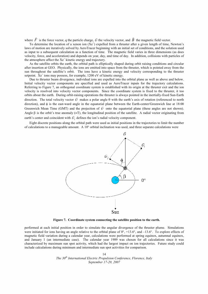
Due to thruster beam divergence, individual ions are expelled into the orbital plane as well as above and below. Initial velocity vector components are specified and used as AeroTracer inputs for the trajectory calculations. Referring to Figure 7, an orthogonal coordinate system is established with its origin at the thruster exit and the ion velocity is resolved into velocity vector components. Since the coordinate system is fixed to the thruster, it too orbits about the earth. During orbit-raising operations the thruster is always pointed in the inertially-fixed Sun-Earth

direction. The total velocity vector υv makes a polar angle θ with the earth’s axis of rotation (referenced to north

direction), and φ is the east-ward angle in the equatorial plane between the Earth-center/Greenwich line at 18:00

Greenwich Mean Time (GMT) and the projection of υv onto the equatorial plane (these angles are not shown).

Angle β is the orbit’s true anomaly (≡T), the longitudinal position of the satellite. A radial vector originating from

earth’s center and coincident with iυv

defines the ion’s radial velocity component.

Eight discrete positions along the orbital path were used as initial positions in the trajectories to limit the number

of calculations to a manageable amount. A 10° orbital inclination was used, and three separate calculations were

Figure 7. Coordinate system connecting the satellite position to the earth.

performed at each initial position in order to simulate the angular divergence of the thruster plume. Simulations

were initiated for ions having an angle relative to the orbital plane of 0°, +13.6°, and –13.6°. To explore effects of magnetic field variation during a calendar year, calculations were performed at spring equinox, autumnal equinox, and January 1 (an intermediate case). The calendar year 1989 was chosen for all calculations since it was characterized by maximum sun spot activity, which had the largest impact on ion trajectories. Future study could include calculations during minimum and intermediate sun spot activities for comparison.

The 30



15

To assess the fate of ions from satellites that are orbit-raised into GEO, calculations were performed for a series of five perigee altitudes from 15,000 km to GEO. Table 6 summarizes the perigee and apogee altitudes used to calculate ion trajectories, and orbital parameters in terms of altitude, latitude, and longitude for each perigee are listed in Table 7. Singly charged xenon-131 (131Xe+) was the only isotope used in this study. The initial ion energy was varied from 300- to 3000-eV although most calculations were completed for mid-range ion energy. Table 5 lists pertinent ion energies and their corresponding velocities. Standard orbital mechanics equations were used to calculate orbital parameters.37-39 An elliptical orbit was assumed with the earth at its focus, characterized by the perigee altitude (hp), apogee altitude (ha), radius of the earth (Re), perigee (rp), and apogee (ra). Perigee and apogee altitudes for the lowest orbit case were taken to be 15,000 km and 47,000 km, respectively (representative orbital parameters when the ion engine begins orbit raising). The velocities at apogee and perigee are related via their radii

a

p

p

a

r

r=

υυ

(8)

Table 6. Perigee and apogee altitudes.

hp (km) ha (km)

42164 114977

40000 109564

25000 72067

20000 59567

15000 47000

Figure 8. Diagram for the discrete satellite positions used in trajectory calculations. The focus of the ellipse

is earth, and satellite positions where ion trajectories were initiated are shown as filled grey circles along the

satellite’s orbital path. The angular measure is indicated along the relative positions of the earth and sun.

The 30



16

Table 7. Orbital parameters for each calculation. The perigee altitude for each set of orbital paths is

indicated by an asterisk.

Altitude (km) Longitude (deg) Latitude (deg)

42164* 0 0.0

62968 90 10.0

71619 105 9.7

81880 120 8.7

93120 135 7.1

114977 180 0.0

93120 225 -7.1

62968 270 -10.0

40000* 0 0.0

59876 90 10.0

68141 105 9.7

77944 120 8.7

88683 135 7.1

109564 180 0.0

88683 225 -7.1

59876 270 -10.0

25000* 0 0.0

38448 90 10.0

44040 105 9.7

50673 120 8.7

57939 135 7.1

72067 180 0.0

57939 225 -7.1

38448 270 -10.0

20000* 0 0.0

31305 90 10.0

36006 105 9.7

41582 120 8.7

47690 135 7.1

59567 180 0.0

47690 225 -7.1

31305 270 -10.0

15000* 0 0.0

24151 90 10.0

27955 105 9.7

32464 120 8.7

37403 135 7.1

47000 180 0.0

37403 225 -7.1

24151 270 -10.0

The 30



17

so that

ea

ep

a

p

p

a

Rh

Rh

r

r

+

+==

υυ

., (9)

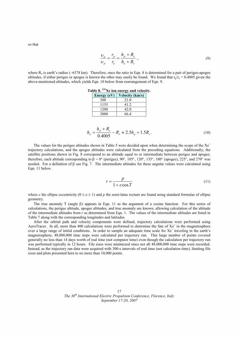
where Re is earth’s radius (~6378 km). Therefore, once the ratio in Eqn. 8 is determined for a pair of perigee-apogee altitudes, if either perigee or apogee is known the other may easily be found. We found that rp/ra = 0.4005 given the above-mentioned altitudes, which yields Eqn. 10 below from rearrangement of Eqn. 9.

Table 8. 131Xe ion energy and velocity.

Energy (eV) Velocity (km/s)

300 21.0

1155 41.2

1200 42.0

3000 66.4

epe

ep

a RhRRh

h 5.15.24005.0

+≈−+

= . (10)

The values for the perigee altitudes shown in Table 5 were decided upon when determining the scope of the Xe+ trajectory calculations, and the apogee altitudes were calculated from the preceding equations. Additionally, the satellite positions shown in Fig. 8 correspond to an altitude equal to or intermediate between perigee and apogee;

therefore, each altitude corresponding to β = 0° (perigee), 90°, 105°, 120°, 135°, 180° (apogee), 225°, and 270° was

needed. For a definition of β see Fig. 7. The intermediate altitudes for these angular values were calculated using Eqn. 11 below.

Te

pr

cos1+= (11)

where e the ellipse eccentricity (0 ≤ e ≤ 1) and p the semi-latus rectum are found using standard formulas of ellipse geometry.

The true anomaly T (angle β) appears in Eqn. 11 as the argument of a cosine function. For this series of calculations, the perigee altitude, apogee altitudes, and true anomaly are known, allowing calculation of the altitude of the intermediate altitudes from r as determined from Eqn. 1. The values of the intermediate altitudes are listed in Table 7 along with the corresponding longitudes and latitudes.

After the orbital path and velocity components were defined, trajectory calculations were performed using AeroTracer. In all, more than 400 calculations were performed to determine the fate of Xe+ in the magnetosphere over a large range of initial conditions. In order to sample an adequate time scale for Xe+ traveling in the earth’s magnetosphere, 48,000,000 time steps were calculated per trajectory run. This large number of points covered generally no less than 14 days worth of real time (not computer time) even though the calculation per trajectory run was performed typically in 12 hours. File sizes were minimized since not all 48,000,000 time steps were recorded. Instead, as the trajectory ran data were acquired with 300-s intervals of real time (not calculation time), limiting file sizes and plots presented here to no more than 10,000 points.

The 30



18

Figure 9. Altitude plots for ion trajectories initiated at orbital locations shown by the black dot on the ellipse

with longitudinal (true anomaly) values for panels with longitudes of (a) 0°°°° (perigee), (b) 90°°°°, (c) 105°°°°, (d) 120°°°°, (e) 135°°°°, (f) 180°°°° (apogee), (g) 225°°°°, and (h) 270°°°°. The same orbital path orientation is used here as in

Figure 8. Plotted are altitude variations in time for Xe+ at hp = 15000 km with 1155 eV during the spring

equinox.

The 30



19

Figure 10. Trajectory plots for hp = 15,000 km and 1155 eV ion energy initiated at ββββ = 0°°°° during the 1989 spring equinox.

Sun

Satellite orbit

Earth

Xe+ trajectory

Sun

Earth

Xe+ trajectory

Magnetosphere boundary

ββββ = 0°°°°

The 30



20

Figure 11. Trajectory plots for hp = 15,000 km and 1155 eV ion energy initiated at (above) ββββ = 0°°°° and (below) ββββ = 120°°°°, during the 1989 spring equinox.

The 30



21

Figure 12. Trajectory plot for hp = 15,000 km and 1155 eV ion energy initiated at ββββ = 120°°°° during the 1989 spring equinox.

ββββ = 120°°°°

The 30



22

Figure 13. (a) Trajectory plot for hp = 15,000 km and 1155 eV ion energy initiated at (above) ββββ = 135°°°° and (below) ββββ = 225°°°° during the 1989 spring equinox.

The 30



23

Table 8. Termination status conditions for selected Xe+ trajectories.

Spring Equinox Autumnal Equinox January 1

Altitude (km) 1. Xe+ in

orbit plane

Xe+ above

orbit plane Xe

+ below

orbit plane 2. Xe+ in

orbit plane

Xe+ above

orbit plane Xe

+ below

orbit plane 3. Xe+ in

orbit plane

Xe+ above

orbit plane Xe

+ below

orbit plane

42164 (perigee) Outside Outside Outside Outside Outside Outside Outside Outside Outside

62968 Outside Outside Outside Outside Outside Outside Outside Outside Outside




40000 (perigee) Max Steps Max Steps Max Steps Outside Outside Outside Max Steps Max Steps Max Steps





25000 (perigee) Max Steps Max Steps Max Steps Max Steps Max Steps Max Steps Max Steps Max Steps Max Steps

38448 Outside Outside Outside Outside Outside Outside Max Steps Outside Outside

44040 Max Steps Outside Outside Outside Outside Max Steps Outside Outside Outside

50673 Outside Outside Max Steps Outside Outside Outside Outside Outside Outside




38448 Max Steps Max Steps Max Steps Max Steps Max Steps Max Steps Outside Outside Outside


31305 Max Steps Max Steps Max Steps Max Steps Max Steps Max Steps Max Steps Max Steps Max Steps

36006 Max Steps Outside Outside Outside Outside Outside Max Steps Outside Max Steps

41582 Outside Outside Outside Outside Outside Outside Max Steps Outside Outside



47690 Outside Outside Outside Outside Outside Outside Outside Max Steps Outside





32464 Outside Max Steps Max Steps Max Steps Max Steps Max Steps Max Steps Max Steps Max Steps

37403 Outside Outside Outside Max Steps Max Steps Outside Outside Outside Max Steps

47000 Outside Outside Outside Outside Max Steps Max Steps Max Steps Max Steps Max Steps


24151 Max Steps Max Steps Max Steps Outside Max Steps Max Steps Max Steps Max Steps Max Steps

For each calculation, the output gathered was a plot of the ion trajectory and three-dimensional coordinates for

the ion position as a function of time. The time-dependent position information was transformed into altitude and plotted as shown in Figure 9. The ordinate values are the ion’s altitude given in reduced units of earth radii Re (1 Re = 6378 km). The abscissa is time in units of days. In the upper portion of each panel, the satellite orbital position shown in Fig. 8 has been reproduced as the small inset. Instead of showing eight circles along the orbital path, only one circle is present. This solitary filled circle denotes the satellite position where the Xe+ are produced and,

The 30



24

therefore, the initiation position of the trajectory calculation. The plotted curves represent the altitude variation in time for Xe+.

The results shown graphically in Figure 9 are typical for the vast majority of trajectory cases studied. Trajectory stability is characterized by fluctuation in altitude. In a given satellite orbit, Xe+ trajectories are most stable when initiated near perigee, (Fig. 9a), become less stable as the satellite altitude is increased (Figs 9b – 9d), and are least stable at apogee (Fig. 9f). The least stable trajectories terminate either by effectively exiting the earth magnetosphere (Figs. 9e and 9f) or traveling to within a minimal altitude, defined as 30 km. Most simulations show that Xe+ trajectories become unstable within two weeks and exit the magnetosphere within this time period. The time between Xe+ emission from the thruster and exiting the magnetosphere decreases with increasing altitude. Very few cases terminate due to reaching the minimum altitude condition. As yet, no systematic characteristics have been identified to explain trajectories terminating below 30 km. More detailed examination of the conditions leading to near-earth (within 30 km of earth’s surface) Xe+ trajectories should be performed but were beyond time limitations of this study.

To produce a termination status during a trajectory calculation based on exiting the magnetosphere, the altitude

must reach at least 10 Re for the position closest to the sun on the sun-side of the earth (270° longitude at 18:00 GMT) while larger altitudes are needed in the magnetotail regions. The tail distance was limited to 100 Re for termination purposes.The altitude results shown in Fig. 9 were for trajectory calculations initiated at 15,000 km perigee altitude and Xe+ kinetic energy of 1155 eV at spring equinox. These are the most stable results, with higher perigee altitudes exhibiting shorter-lived stable trajectories along the satellite’s orbital path. Selected trajectory results corresponding to the plots of Fig. 9 are presented in the subsequent figures. The axes are in reduced units of earth’s radius, Re. The trajectory plots of Figs. 10 and 12 contain two panels displaying projections of the three-dimensional trajectory in two-dimensional planes. The upper panel displays the trajectory projected on the noon-midnight meridional plane (north-south projection), and the lower panel shows the projection on the equatorial plane (looking down from the north pole toward the south pole). Note that not all calculated points are displayed. Recall that each calculation consisted of up to 48,000,000 time steps, but only points spaced at 300 seconds are plotted, greatly decreasing the congestion within the plots. The three-dimensional plot of Fig. 11 (upper) displays the same results as the two panels of Fig. 10, for comparison. Similarly, the lower plot of Fig. 11 corresponds to the two panels of Fig. 12.

Figure 10 contains labels for the sun and earth positions, the satellite orbital track, and Xe+ trajectory starting

from 0° longitude with the earth positioned at 18:00 GMT. Each revolution the Xe+ takes around the earth is shown as a different color. The revolutions are colored black, green, and red for the first, second, and third revolutions, respectively.

Again, the trajectories shown in Figs. 10-13 with altitudes plotted in Fig. 9 are typical of ion trajectory

instabilities produced at increasing altitudes. The smooth, circular orbit established from perigee (β = 0°) in Fig. 10

(altitude profile in Fig. 9a) is degraded from orbits initiated at β = 90° and greater until apogee is reached, and then

begins to become more stable at β > 180°. Although one might assume that trajectories initiated at nearly identical positions but on opposite sides of the

orbital path (e.g., β = {90°, 270°} or β = {135°, 225}) will be similar, the results show clear deviations in the trajectories. The dissimilarity between these trajectories is expected based on the highly anisotropic magnetic field

structure about earth. As evidenced in altitude plots shown in Fig. 9, trajectories initiated for 0° < β < 180° show

larger altitude fluctuations than do those for 180° < β < 360°.At low perigee altitudes (15,000km and 20,000 km), many of the trajectories are quite stable and continue to orbit around earth in excess of two weeks. The most stable trajectories were studied for longer amounts of time and found to have stable circular trajectories in excess of 46 days, the longest the calculation was allowed to run.

Table 7 summarizes the termination status for Xe+ trajectories. The column headings specify the relative epoch

and initial Xe+ ejection angle with respect to the satellite orbital plane. Ions exhausted from the thruster at +13.6° or

–13.6° are labeled as above or below orbit plane, respectively, in the table. As indicated in the altitude column, each perigee altitude begins a sub array in the table, and subsequent sub arrays have alternating grey or white shading for their altitude entries.

As an estimate of the probability for the various termination events for ions expelled during the orbit transfer, we divide the number of occurrences for each by the total. The result (see Table 8) suggests low probability for re-capture in the near-Earth atmosphere and a 38% probability for Earth-orbit capture at an altitude of ~several Earth radii. The estimated probability for losing ions from earth orbit is 62%. Fast neutrals exiting the thruster and not directed toward Earth are lost to space, however these constitute less than 1% of the exhaust.

The 30



25

Table 9. Occurrences and Estimated Probability for Termination Events.

Minimum

Altitude

Maximum Steps Outside

Magnetosphere

Total

# of Occurrences 0 117 189 306 Probability 0.0 0.38 0.62 1.00

F. Atmospheric Charged Particle Density, Circulation, and Loss

Ions and electrons have been injected artificially into the Earth’s atmosphere at various altitudes, as a result of nuclear tests.40 The decay of most of the radioactive nuclei formed releases electrons of MeV-level average energy, with a very high initial release rate that decreases exponentially. A pair of nuclear explosions in August 1958 at 80- and 43-km altitude, respectively, produced an almost instantaneous aurora near the explosion and a second aurora about 2000 miles away a minute later. It was concluded that most of the electrons were trapped in the earth’s magnetic field and spiraling back and forth between mirror points. A few days later most electrons had apparently suffered collisional scattering and absorption by the atmosphere. Also in 1958, three small nuclear explosions at about 500 km altitude, each separated by a few days produced a well-defined radiation belt about 100 km thick extending between 1.7 and 2.2 Re. The electrons leaked out over a period of several weeks. This lifetime did not change significantly with altitude. The much larger Starfish explosion at 400-km altitude produced immediate auroras at the site and 5000 km away. A radiation belt with a lifetime measured in years was created, and several satellites became inoperable due to solar cell damage. Geomagnetic field disturbances and disruptions in radio communications affected large areas for days. Increased levels of ionization were produced in the ionosphere, and electrons were introduced into the upper atmosphere also, at much higher altitudes than the explosion occurred. Proton flux levels in the Earth’s inner radiation belt were disturbed over a period of several months; the pre-existing distribution of trapped protons was apparently modified. Electron flux was as high as 109/cm2-sec. Decay of the artificially produced electrons occurred at 1.2 to 1.7 Re with lifetime of several years, and several months for 2.5 Re. Reactions with atmospheric atoms are considered ineffective in removing electrons beyond 1.7 Re, and the explanation for this lifetime variation with altitude is uncertain.

G. Xenon Chemistry and Potential Environmental Impacts of EP Effluents

In the troposphere there are no environmental standards for xenon, since there are no perceived negative impacts large enough to warrant it. Likewise, there are no EPA, state, local or international regulations of other noble gases.

Xenon is inert towards the vast majority of other atoms and molecules, consistent with its classification as a noble gas. Since the valence electron shells of noble (or rare) gases are filled, they have high ionization energy and very low electron affinity, and do not readily participate in chemical bonding. The lightest rare gases, helium and neon, are the only elements for which stable chemically bound molecules have not been identified. Xenon reacts with fluorine gas to form xenon fluorides, and various oxides, acids and salts can be formed. HXeF, and more generally HXeY, where Y is an electronegative fragment, is one type of xenon compound. These molecules derive their stability from (HXe+Y-) ionic configurations, as do molecules of the type XeYx.

The first chemical compound discovered that involves a noble gas atom is XePtF6, reported in 1962. It exists as an octahedral anionic fluoride complex involving cations of xenon-fluorides. The first binary compound discovered containing a noble gas was XeF4, a white moisture-sensitive solid formed via an exothermic reaction (251 kJ per xenon mole). Xenon difluoride is a powerful fluorinating agent, formed via the reaction

22 XeFFXe →+ (12)

in the presence of an energy input such as heat, irradiation, or a electrical discharge. Even sunlight is sufficient to enable the reaction at atmospheric pressure. XeF2 is corrosive, highly toxic, an explosion hazard, and yet one of the

most stable xenon compounds. It is a gas above -30 °C. XeF6 has a much more complicated structure than the other xenon fluorides, but like them reacts rapidly with water and moist air. For both XeF6 and XeF4 this reaction produces XeO3 and HF directly. The xenon trioxide is a very powerful oxidizing agent. Under certain conditions it

is explosive. XeO4 is even more unstable, decomposing explosively above -35.9 °C. to transform itself into a

The 30



26

gaseous mix of xenon, O2 and O3 (ozone). The synthesis of XeO4 starts from XeO64-, called perxenate, and one of

the two known pathways uses ozone to oxidize a xenate (XeO42-) in solution

2

4

63

2

4 22242 OXeOOeXeO +→++ −−− . (13)

Xenon forms a very wide variety of compounds of the type XeOxY2, where x = 1-3 and Y is an electronegative

group such as CF3. Accounting for the details of atmospheric chemistry is extremely complex, however the natural occurrence of

xenate in the atmosphere has not been reported and therefore it can be concluded that reaction (13) is very likely an insignificant ozone loss mechanism.

Upper atmosphere ozone is formed primarily through the reaction

MOMOPO +→++ 32

3 )( , (14)

where M is a third body collision partner. The O(3P) atoms are obtained from the photodissociation of oxygen via

),,()( 133

2 etcDPOPOhO +→+ ν (15)

where the oxygen atom electronic state distribution is influenced by the wavelength spectrum of the uv photons. The oxygen atom ground state is 3P and the lowest lying excited state is 1D at 1.97 eV - also the lowest lying metastable level (see Table 10). For photons slightly more energetic than the ~ 242 nanometer wavelength that

corresponds to the 5.12 eV dissociation energy of diatomic oxygen, excitation occurs from the X 3∑g- ground state to

the C 3∆u exited state, the so-called Herzberg band. Given the energy involved, formation of a 1D atom along with 3P in reaction (15) only occurs for λ < 175 nanometers.

The Herzberg-band absorption process is normally prohibited, however certain collisions are effective in removing the prohibition when they occur simultaneous with the excitation. Xenon neutrals, due to their unusually high polarizability, are more effective than other atmospheric collision partners in promoting Herzberg-band absorption. As a result the absorption of uv light by pure O2 has been observed to increase linearly with the partial pressure of added xenon at fixed total pressure,41 and the ozone concentration formed showed the same linear dependence on partial pressure. The presence of ground-state neutral xenon, the predominant form in nature, therefore enhances atmospheric ozone production.

Xenon also exists in metastable, ionized, and excimer forms. As a dimer xenon may exist as Xe2* and as Xe2+.

As the largest of the noble gas atoms (except for the short-lived radon due to its radioactive decay), xenon has the lowest ionization and metastable energies of the group. In a mixture of noble gases, excitation energy will therefore be efficiently transferred to xenon. Similarly, in the atmosphere, xenon and other excitation energy will flow toward excitation of N, O, and N2 metastables and the dissociation of oxygen molecules (and nitrogen molecules to a lesser extent), as suggested by the energetic properties listed in Table 10.

The primary sources of excitation in the upper atmosphere are absorption of solar uv radiation and collisions with energetic electrons. Electric thruster exhaust already contains energetic xenon species, however, in the form of Xe+, Xe2+, Xe* and fast Xe. Fast Xe atoms have high kinetic energy, and are produced when an exhaust ion undergoes a charge exchange reaction and becomes neutralized. The original momentum of the xenon particle is retained, so that these species have the original exhaust velocity and energy of the ion, typically on the order of 42 km/s and 1200 eV. Through collisions of expelled ions and fast neutrals with atmospheric species, kinetic energy will be transferred, with the inevitable production of many O atoms that proceed to form ozone via reaction (14).

Ozone is destroyed at high altitudes via

23 2 OOO →+ , (16)

and at low altitudes42 (below 40 km) via

The 30



27

22

223

ONOONO

ONOONO

+→+

+→+ (17)

Excited-state O atoms are converted quickly to ground-state species via collisions with O2 and other atmospheric collision partners. As a result, increased production of O atoms raises production and destruction rates for ozone by comparable amounts and has minimal effect on ozone concentration. The destruction of ozone may also occur via collisions with Xe*, Xe+, Xe2+, and fast Xe, however there is no available data concerning this. The very low dissociation energy of ozone (see Table 10) could be an important factor concerning the ozone rate of destruction caused by collisional events.

Table 10. Properties of Selected Atmospheric Species

*Very large energy, hence formation of Xe22+ is improbable and considered insignificant here.

**Many of the excited electronic states are poorly characterized. N/A = not applicable (dissociation energy does not pertain to single atoms).

Because xenon is naturally present in the atmosphere, and not produced or destroyed in any significant way, it

maintains a constant volume and weight fraction in the well-mixed region below 90 km. Xenon released in the troposphere will diffuse slowly into the remainder of the atmosphere. With natural sea-level concentration of 0.48 kg/km3, catastrophic release of the contents of a xenon propellant tank containing 250 kg has to uniformly diffuse

into approximately 500 km3 of sea-level air to equal the natural abundance. Since earth has 5.1×108 km2 of surface

area, the atmospheric volume to 1-km altitude is 5.1×108 km3, or ~1 million times the diffusion volume mentioned above. Therefore, the catastrophic release increases the xenon concentration by ~1 ppm if uniformly diffused to an altitude of 1 km. The time required to effect world-wide diffusion would be considerable, on the order of weeks or months and depending on global circulation patterns, storms, etc.43

Neutral xenon released into the atmosphere can be ionized by several possible mechanisms: (1) photoionization due to solar ultraviolet radiation, (2) impact ionization through collisions with other atomic species or electrons, and (3) charge exchange collisions with ambient ions (especially O+ within the exosphere and H+ at higher altitudes (see Fig. 1)).

When the wavelength-dependent xenon photoionization cross section and solar spectral flux are convolved, the

calculated time constant for Xe ionization in sunlight44 is 2.2 × 105 seconds or about 61 hours. For a constant release rate R of neutral xenon in atoms per second, the total number of Xe+ produced at time t can be estimated from

))102.2/exp(1( 5×−− tRt . (18)

The cross section for charge-exchange collisions of Xe atoms with O+ ions is σce ≈ 2×10-15 cm2,45 less than the elastic-collision cross section. The Xe+ production rate can be estimated from

XeOce nvnP += σ , (19)

Atom or

Molecule

Mass (amu; natural

isotopic abundance)

Ionization

Energy (eV)

Lowest Metastable

Energy (eV)

Dissociation

Energy (eV)

Xenon 131.293 12.13 8.32b N/A

Argon 39.948 15.76 11.55 N/A

N atom 14.007 14.53 2.38 N/A

O atom 16.001 13.62 1.97 N/A

N2 28.014 15.58 6.2 9.76

O2 32.001 12.07 0.98 5.12

Xe2 262.59 11.1 ** 0.023

Xe2+ 262.59 * ** 1.03

O3 48.002 12.70 1.2 0.76

The 30



28

where the brackets denote average values and v is relative Xe – O+ velocity. After integrating over time and volume, and assuming constant release rate, the total number of Xe ions formed is45

25102 RtN

Xe

−×≈+ (20)

if the O+ density is 105 cm-3 and relative velocity v is 5×105 cm/s (a representative spacecraft velocity). A similar type of calculation for the case of electron impact production of Xe+ produces the result

210102 RtN

Xe

−×≈+ , (21)

assuming the electron temperature is as high as 1 eV and ne = 105 cm-3. Obviously, the production rate due to charge exchange is much higher than electron impact production for these assumptions. Since the electron temperature is normally lower, ion production via thermal electron impact is negligible. For monoatomic ions at ionospheric

temperatures (1000 °K), the radiative recombination coefficient is typically on the order of 10-12 cm3s-1.46 If radiative recombination dominates the Xe+ loss process, then even upper atmosphere solar photoionization of xenon occurs at a faster rate than the ions are lost. Within the exosphere charge transfer ionization of xenon is much faster than photoionization, but in geostationary earth orbit (GEO), charge transfer can be neglected due to the very low densities of prospective collision partners. The recombination rate at GEO also is much less than in the lower atmosphere. Therefore it is anticipated that most xenon neutrals released over essentially the entire range of ion engine operating altitudes will be converted to the ionized form. In addition to charge exchange collisions, xenon neutrals undergo elastic collisions with ambient plasma ions, causing these ions to scatter. Sizable release of neutral atoms and molecules during a brief period of time causes measurable perturbation of ionospheric plasma density.47

III. Concluding Remarks

Few measurement data exist concerning the atmospheric distribution of xenon, therefore this distribution has been calculated. Although the plume concentration near the thruster is much greater than natural abundance levels, the increase in atmospheric concentration due to its release from an ion thruster is shown to be small at all altitudes, even for volumes of modest size. In the worst case - rapid release of the entire contents of the propellant tank, after a short diffusion period measured in hours the natural abundance will dominate. Neutral atoms released from the thrusters can be ionized via several mechanisms. These rates are considered in the paper, and it is concluded that at each operational altitude xenon will exist predominantly in the ionized form.

It is shown that eroded species emitted from xenon electric thrusters, after a modest amount of atmospheric transport and mixing, are always relatively insignificant in comparison to natural sources.

Xenon is a noble gas, but due to its position in the periodic table is more reactive than other noble gases. A consideration of its atmospheric chemistry and environment suggest that some potential for chemical reactions exists, and this may merit further study.

Xenon ion thrusters typically serve multiple functions. The initial function is orbit raising, however on-orbit stationkeeping and other functions must also be performed. In each case, thruster orientation with respect to the earth-sun direction varies. In addition, other factors influence the trajectories of emitted ions, such as the magnitude of ion velocity and the local magnetic field amplitude and direction. These factors depend on spacecraft position (latitude, longitude, altitude) for thruster firing, time of year, etc.

Ion trajectories from the spacecraft have been calculated using AeroTracer, a code that computes the motion of charged particles by applying an adaptive step-size Runge-Kutta technique to the fully relativistic Lorentz equation. Based on the simulation results, at most only a small fraction of the ions will return directly to the troposphere. Many are lost from the atmosphere, i.e. they trip a termination condition by traveling to an altitude outside the earth’s magnetosphere. Roughly one-third of the ions enter an earth orbit that is stable on the time scale for which the computations can reasonably be performed. These ions are likely to undergo collisional events that result in significant loss of kinetic energy and/or charge exchange leading to production of neutral xenon. In either case, xenon retention in the atmosphere seems likely.

The 30



29

It is clear that use of xenon electric propulsion is a better choice, from an environmental standpoint, than the conventional approach that relies on hydrazine. While some xenon, certainly a finite resource, is irretrievably lost to space, the loss fraction for a single launch of the class considered is negligible.

Acknowledgments

Dr. M. McNab of the Aerospace Space Science Applications Laboratory is the developer of the AeroTracer program. The authors are grateful for his assistance in learning how to use the code and revising one aspect of the program. MWC acknowledges useful discussions with J.E. Pollard and B.B. Brady. Preparation of this manuscript was supported under The Aerospace Corporation’s Independent Research and Development Program.

References

1F.C. Wilson, “Recent Advances in Satellite Propulsion and Associated Mission Benefits,” AIAA-2006-5307, International

Communications Satellite System Conference, San Diego, June 2006. 2M. Martinez-Sanchez and J.E. Pollard, “Spacecraft Electric Propulsion – An Overview,” J. Propulsion and Power, Vol. 14,

No. 5, Sept-Oct 1998. 3T.P. Garrison, M. Ince, J. Pizzicaroli, and P.A. Swan, “Systems Engineering Trades for the IRIDIUM Constellation,” J.

Spacecraft and Rockets, Vol. 34, No. 51997, pp. 675-80. 4J.E. Pollard and S.W. Janson, “Spacecraft Electric Propulsion Applications,” ATR-96(8201)-1 (Aerospace Corporation, El

Segundo, CA), February 1996. 5G.P. Sutton, Rocket Propulsion Elements, 6th ed. (John Wiley & Sons, New York), 1992. 6R.G. Jahn and E.Y. Choueiri, “Electric Propulsion” in Encyclopedia of Physical Science and Technology, 3rd Ed., Vol. 5

(Academic Press), 2002. 7P.A. Zbinden, M.A. Hidalgo, P. Eberhardt, and J. Geiss, “Mass Spectrometer Measurements of the Positive Ion Composition

in the D- and E-Regions of the Ionosphere,” Planet. Space Sci., Vol. 23, pp. 1621-42, 1975. 8W.J. McNeil, S.T. Lai, and E. Murad, “Differential Ablation of Cosmic Dust and Implications for the Relative Abundances

of Atmospheric Metals,” J. Geophys. Res., Vol. 103, No. D9, 1998, pp. 10899-911. 9Mason, B. (ed.), Handbook of Elemental Abundances in Meteorites, Gordon and Breach, New York, 1971. 10S.G. Love and D.E. Brownlee, “A Direct Measurement of the Terrestrial Mass Accretion Rate of Cosmic Dust,” Science,

Vol. 262, 1993, p. 550. 11D.W. Hughes, “Cosmic Dust Influx to the Earth,” Adv. Space Res., Vol. XV, 1975, pp. 531-9. 12J.M. Grebowsky and M.W. Pharo III, “The Source of Midlatitude Metallic Ions at F-Region Altitudes,” Planet. Space Sci.,

Vol. 33, No. 7, 1985, pp. 807-815. 13Emsley, J., The Elements, 2nd ed., Clarendon Press, Oxford, 1991. 14J.A. Ratcliffe, An Introduction to the Ionosphere and Magnetosphere (Cambridge University Press, London), 1972. 15M.G. Kivelson and C.T. Russell, eds., Introduction to Space Physics (Cambridge University Press, New York), 1995. 16I.A. Daglis, R.M. Thorne, W. Baumjohann, and S. Orsini, “The Terrestrial Ring Current: Origin, Formation, and Decay,”

Reviews of Geophysics, Vol. 37, No. 4, 1999, pp. 407-438. 17S. Matsushita, “A Study of the Morphology of Ionospheric Storms,” J. Geophys. Res., Vol. 64, No. 3, 1959, pp. 305-32 18C.Y. Johnson, “Ion and Neutral Composition of the Ionosphere,” Annals of the IQSY, Vol. 5, pp. 197-213, 1969. 19International Reference Ionosphere: http://modelweb.gsfc.nasa.gov/models/iri.html 20MSISE Atmosphere Model: http://modelweb.gsfc.nasa.gov/models/msis.html 21Lide, David R. Handbook of Chemistry and Physics, Boca Raton, FL: CRC, 1996: 14-7. 22Anon, “U.S. Standard Atmosphere, 1962,” COESA product (Washington, USGPO, Dec 1962), sponsored by

NASA/USAF/USWB. 23J.L. Fox, “Ar+ in the Terrestrial Ionosphere,” J. Geophys. Res., Vol. 91, No. A2, 1986, pp. 1731-3. 24D. Hayashi, G. Heusler, G. Hagelaar, and G. Kroesen, “Discharge Efficiency in High-Xe-Content Plasma Display Panels,”

J. Appl. Phys., Vol. 95, No. 4, 2004, pp. 1656-61. 25R.O. Jung, J.B. Boffard, L.W. Anderson, and C.C. Lin, “Electron-Impact Excitation Cross Sections from the Xenon J=2

Metastable Level,” Phys. Rev. A, Vol. 72, 022723, 2005. 26Personal communication, Earlene Schillingford. 27R.P. Welle, “Availability Considerations in the Selection of Inert Propellants for Ion Engines,” Paper 90-2589, 21st

International Electric Propulsion Conference, Orlando, July 1990; ibid, “Noble Gas Use for Electric Space Propulsion,” CryoGas International, Vol. 31, No. 4, p. 9, April 1993.

28International Association of Geomagnetism and Aeronomy, http://www.ngdc.noaa.gov/IAGA/vmod/igrf.html. 29N. A. Tsyganenko, Planet. Space Sci. 37, 5-20, 1989. 30N. A. Tsyganenko, J. Geophys.Res., 107, A8, 10.1029/2001JA000219, 2002.

The 30



30

31N. A. Tsyganenko, H. J. Singer, and J. C. Kasper, Storm-time distortion of the inner magnetosphere: How severe can it get? J. Geophys.Res., 108, A5, 10.1029/2002JA009808, 2003.

32N. A. Tsyganenko and M. I. Sitnov, J. Geophys.Res., 110, A3, 10.1029/2004JA010798, 2005. 33A. Spitzer, “Novel Orbit Raising Strategy makes Low Thrust Commercially Viable,” IEPC Paper, 95-212, 24th International

Electric Propulsion Conference, Moscow, Sept. 1995. 34D.M. Goebel, M. Martinez-Lavin, T.A. Bond, and A.M. King, “Performance of XIPS Electric Propulsion in On-orbit

Station Keeping of the Boeing 702 Spacecraft,” AIAA Paper 2002-4348, 38th Joint Propulsion Conference, Indianapolis, July 2002.

35N.E. Goodzeit and S. Ratan, “System for High Efficiency Spacecraft Orbit Transfer,” U.S. Patent No. 6845950, Jan. 2005. 36B.M. Anzel, Y.M. Ho, and R.A. Noyola, “Fuel Efficient Methods for Satellite Stationkeeping and Momentum Dumping,”

U.S. Patent No. 6015116, Jan. 2000. 37V.A. Chobotov (ed.), Orbital Mechanics, 3rd ed., (American Institute of Aeronautics and Astronautics, Reston, VA), 2002. 38D.A. Vallado, Fundamentals of Astrodynamics and Applications, 2nd ed., (Kluwer Academic Publishers, Boston, 2001). 39R.R. Bate, D.D. Mueller, and J.E. White, Fundamentals of Astrodynamics, (Dover, NY, 1971). 40W.C. Lyon/Hittman Associates, “A Study of Environmental Effects Caused by Cesium from Ion Thrusters,” HIT-487,

contract no. NAS5-11826 for GSFC, March 1971. 41V.I. Andrukhiv et al, “On the Primary Mechanism of Ozone Formation in Oxygen-Containing Mixtures Exposed to

Irradiation with KrF Laser at 248 nm,” Optics and Spectroscopy, Vol. 76, No. 1, 1994, pp. 150-2. 42E. Hesstvedt, “Reduction of Stratospheric Ozone from High-flying Aircraft, Studied in a Two-dimensional Photochemical

Model with Transport,” Can. J. Chem., Vol. 52, 1974, pp. 1592-8. 43R.G. Roble, E.C. Ridley, A.D. Richmond, and R.E. Dickinson, “A Coupled Thermosphere/Ionosphere General Circulation

Model,” Geophys. Res. Lett., Vol. 15, No. 12, 1988, pp. 1325-8. 44E. Wescott, H. Stenbaek-Nielsen, and D. Hampton, “Xenon Critical Velocity Releases from the ACTIVNY Satellite:

Discussion of Attempted Optical Observations,” Geophys. Res. Lett., Vol. 19, 2079-2081, 1992. 45E.Y. Choueiri et al, “Observations and Modeling of Neutral Gas Releases from the APEX Satellite,” J. Geophys. Res., Vol.

106, No. A11, 25673-81, 2001. 46S.J. Bauer, Physics of Planetary Ionospheres, Vol. 6 of Physics and Chemistry in Space, J.G. Roederer, ed. (Springer-

Verlag, New York, 1973). 47P.A. Bernhardt et al, “Lifetime of a Depression in the Plasma Density over Jicamarca produced by Space Shuttle Exhaust in

the Ionosphere,” Radio Sci., Vol. 36, No. 5, 2001, pp. 1209-20.

Documents

Environmental Considerations for Xenon Electric Propulsion