Environmental Chem Data Analysis

8/21/2019 Environmental Chem Data Analysis

http://slidepdf.com/reader/full/environmental-chem-data-analysis 1/7

Data Analysis 1: COD, BOD, and DO

by Anna Le and Kristina Kayatta

Tuesday April 21, 2015



Data Analysis #1 – BOD, COD, DO

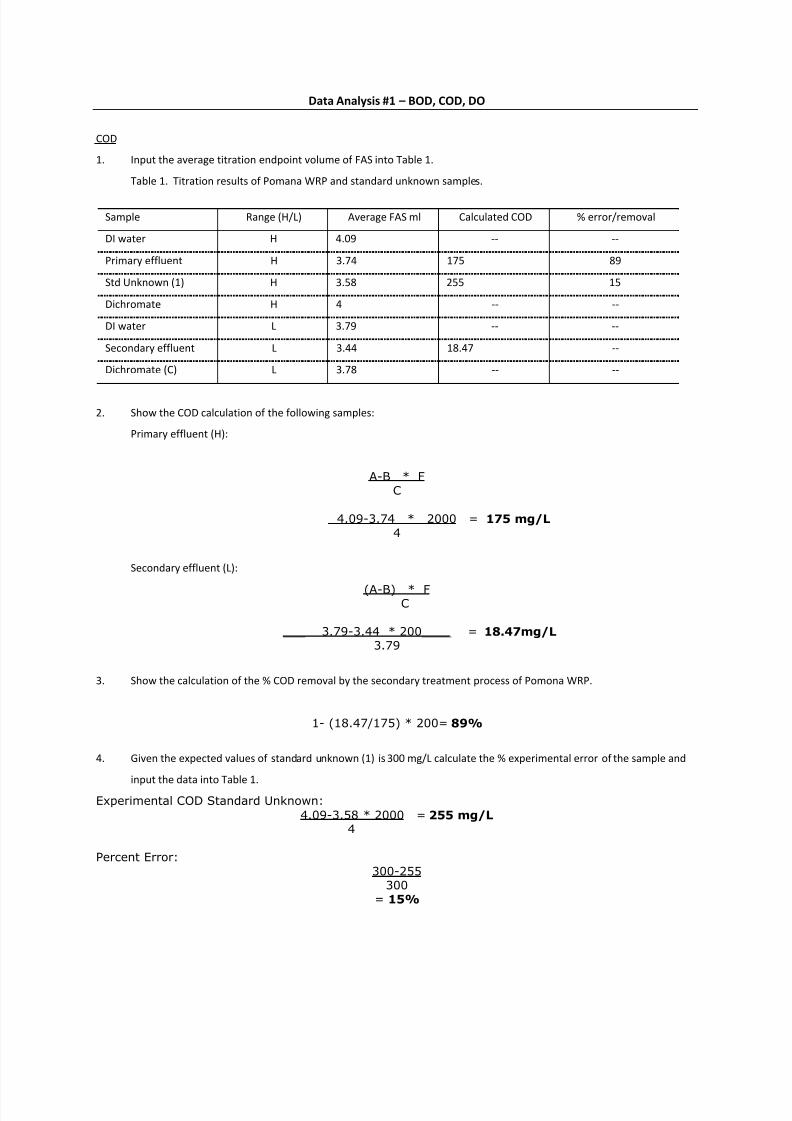
COD

1. Input the average titration endpoint volume of FAS into Table 1.

Table 1. Titration results of Pomana WRP and standard unknown samples.

Sample Range (H/L) Average FAS ml Calculated COD % error/removal

DI water H 4.09 -- --

Primary effluent H 3.74 175 89

Std Unknown (1) H 3.58 255 15

Dichromate H 4 -- --

DI water L 3.79 -- --

Secondary effluent L 3.44 18.47 --

Dichromate (C) L 3.78 -- --

2. Show the COD calculation of the following samples:

Primary effluent (H):

A-B * F

C

4.09-3.74 * 2000 = 175 mg/L

4

Secondary effluent (L):

(A-B) * FC

___ 3.79-3.44 * 200____ = 18.47mg/L

3.79

3. Show the calculation of the % COD removal by the secondary treatment process of Pomona WRP.

1- (18.47/175) * 200= 89%

4. Given the expected values of standard unknown (1) is 300 mg/L calculate the % experimental error of the sample and

input the data into Table 1.

Experimental COD Standard Unknown:

4.09-3.58 * 2000 = 255 mg/L

4

Percent Error:

300-255

300

= 15%



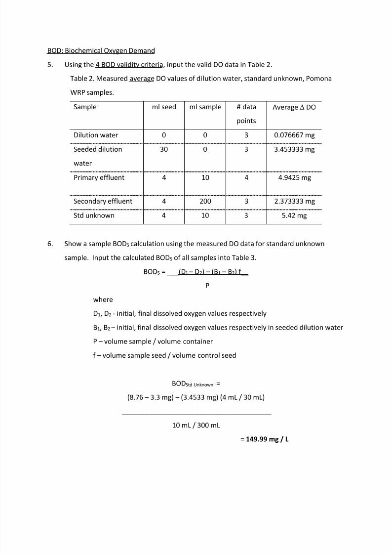
BOD: Biochemical Oxygen Demand

5. Using the 4 BOD validity criteria, input the valid DO data in Table 2.

Table 2. Measured average DO values of dilution water, standard unknown, Pomona

WRP samples.

Sample ml seed ml sample # data

points

Average DO

Dilution water 0 0 3 0.076667 mg

Seeded dilution

water

30 0 3 3.453333 mg

Primary effluent 4 10 4 4.9425 mg

Secondary effluent 4 200 3 2.373333 mg

Std unknown 4 10 3 5.42 mg

6. Show a sample BOD5 calculation using the measured DO data for standard unknown

sample. Input the calculated BOD5 of all samples into Table 3.

BOD5 = ___(D1 – D2) – (B1 – B2) f__

P

where

D1, D2 - initial, final dissolved oxygen values respectively

B1, B2 – initial, final dissolved oxygen values respectively in seeded dilution water

P – volume sample / volume container

f – volume sample seed / volume control seed

BODStd Unknown =

(8.76 – 3.3 mg) – (3.4533 mg) (4 mL / 30 mL)

_______________________________________

10 mL / 300 mL

= 149.99 mg / L



7. Show the calculation of % BOD5 removal by the secondary treatment of Pomona WRP.

Show the calculation of % error in BOD5 analysis based on the standard unknown data,

given the expected BOD5 value was 150 mg/L. Input the results into Table 3.

Average Calculated BOD5 from Secondary Effluent Samples = 2.87 mg/L

Average Calculated BOD5 from Primary Effluent Samples = 134.46 mg/L

% Reduction by Secondary Treatment = ( BODPE - BODSE ) / BODPE

% Reduction = (134.46 mg/L – 2.87 mg/L) / 134.46 mg/L = 97.9%

% Error of Experimental Standard Unknown BOD5 =

|Calculated BOD5 – Actual BOD5| / Actual BOD5

% Error = |148.79 mg/L – 150 mg/L| / 150 mg/L = .008 = 0.8%

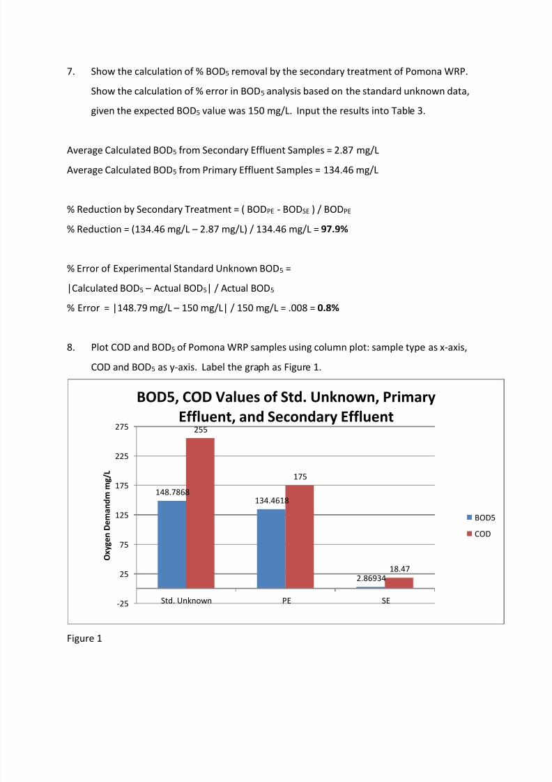
8. Plot COD and BOD5 of Pomona WRP samples using column plot: sample type as x-axis,

COD and BOD5 as y-axis. Label the graph as Figure 1.

Figure 1

148.7868134.4618

2.86934

255

175

18.47

-25

25

75

125

175

225

275

Std. Unknown PE SE

O x y

g e n D e m a n d m m

g / L

BOD5, COD Values of Std. Unknown, Primary

Effluent, and Secondary Effluent

BOD5

COD



9. Calculate the BOD5:COD ratio of the primary and secondary effluent samples and

comment on the results.

Std. Unknown Primary Effluent Secondary Effluent

BOD5 148.7868 134.4618 2.86934

COD 255 175 18.47

BOD5/COD 0.583478 0.768353 0.155351

For the standard unknown sample, 58.35% of the oxygen demand was removed after five days.

This can be interpreted to mean that 58.35% of the organic pollutants were biodegradable.

Likewise, we can interpret our data to mean that 76.8% of the organic matter in the primary

effluent is biodegradable, and 15.5% of the organic matter in the secondary effluent is

biodegradable.

Table 3. Calculated BOD5 results of WRP and standard unknown samples.

Sample Calculated BOD5 (mg/L) % removal/% error

Primary effluent 128.3868, 142.1868, 132.2868,

134.9868

Average = 134.4618

9.63%

Secondary effluent 2.99934, 3.25434, 2.35434

Average = 2.87

97.9%

Std unknown* 149.9868, 248.3868, 146.6868,

149.6868

Average = 148.79

.8%

Dissolved Oxygen (use both sections data)

10. Using the average endpoint volume, show a sample calculation of dissolved oxygen (DO)

from the Winkler titration method.

Dissolved Oxygen (mg/L) = Volume Thiosulfate Titrated (mL)

At room temperature (21 C), the endpoint volumes of Thiosulfate were:

8.80, 8.90, 9.05, 9.10, 9.10, 9.40 mL

DO = ( 8.80 + 8.90 + 9.05 + 9.10 + 9.10 + 9.40 mg/L ) / 6 = 9.05 mg/L



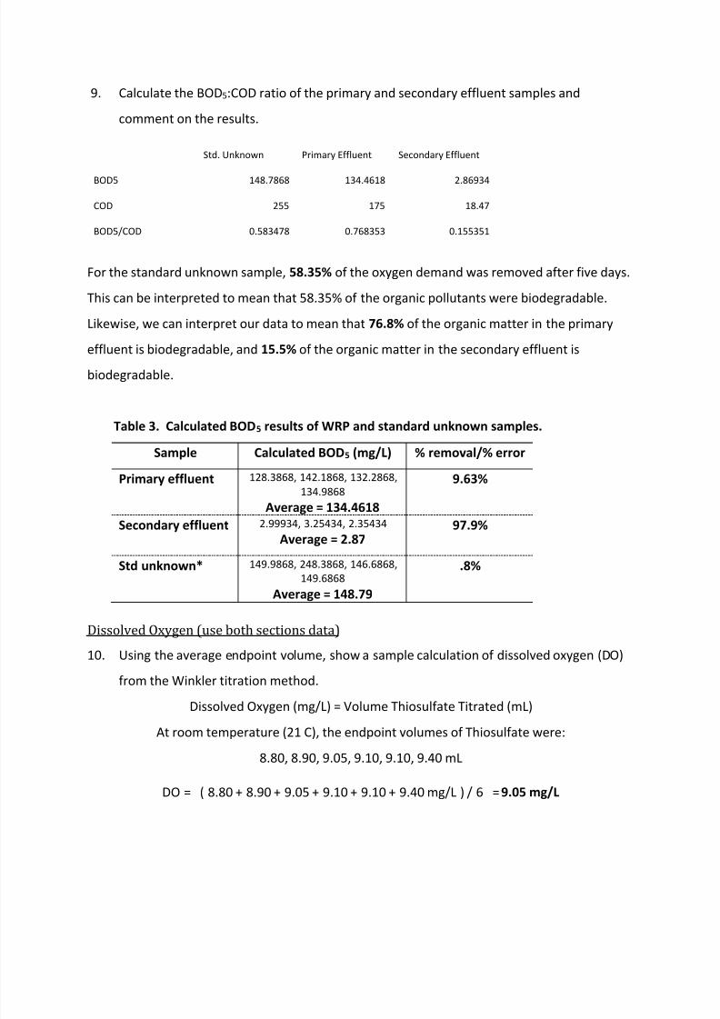
11. Plot the calculated DO (mg/L, y-axis) vs. average measured temperature (oC, x-xis) and

label it as Figure 2. Perform a linear trendline analysis on the data. Comment on the

temperature effects on the solubility of oxygen.

Note: Include major (out) and minor (in) tick marks on both axis; graph size = half page.

Figure 2

4.00

5.00

6.00

7.00

8.00

9.00

10.00

11.00

0 5 10 15 20 25 30 35 40 45 50

D i s s o l v e d O x y g e n ( m g / L )

Temperature (degrees C)

Temperature Effect



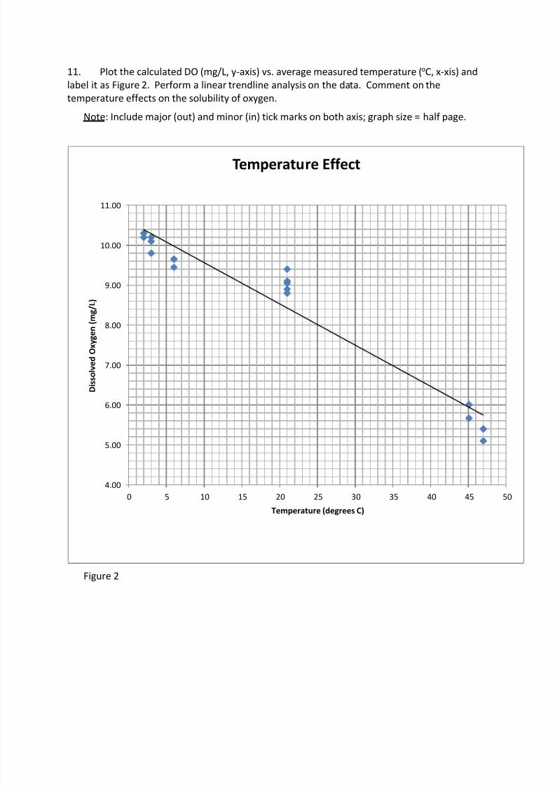
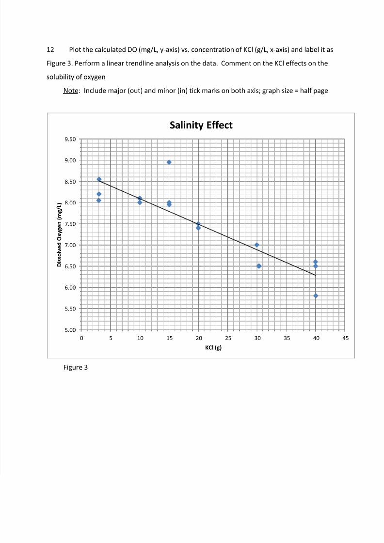
12 Plot the calculated DO (mg/L, y-axis) vs. concentration of KCl (g/L, x-axis) and label it as

Figure 3. Perform a linear trendline analysis on the data. Comment on the KCl effects on the

solubility of oxygen

Note: Include major (out) and minor (in) tick marks on both axis; graph size = half page

Figure 3

5.00

5.50

6.00

6.50

7.00

7.50

8.00

8.50

9.00

9.50

0 5 10 15 20 25 30 35 40 45

D i s s o l v e d O x y g e n ( m g / L )

KCl (g)

Salinity Effect

Documents

Environmental Chem Data Analysis