Environment MappingCSE 781 – Roger Crawfis

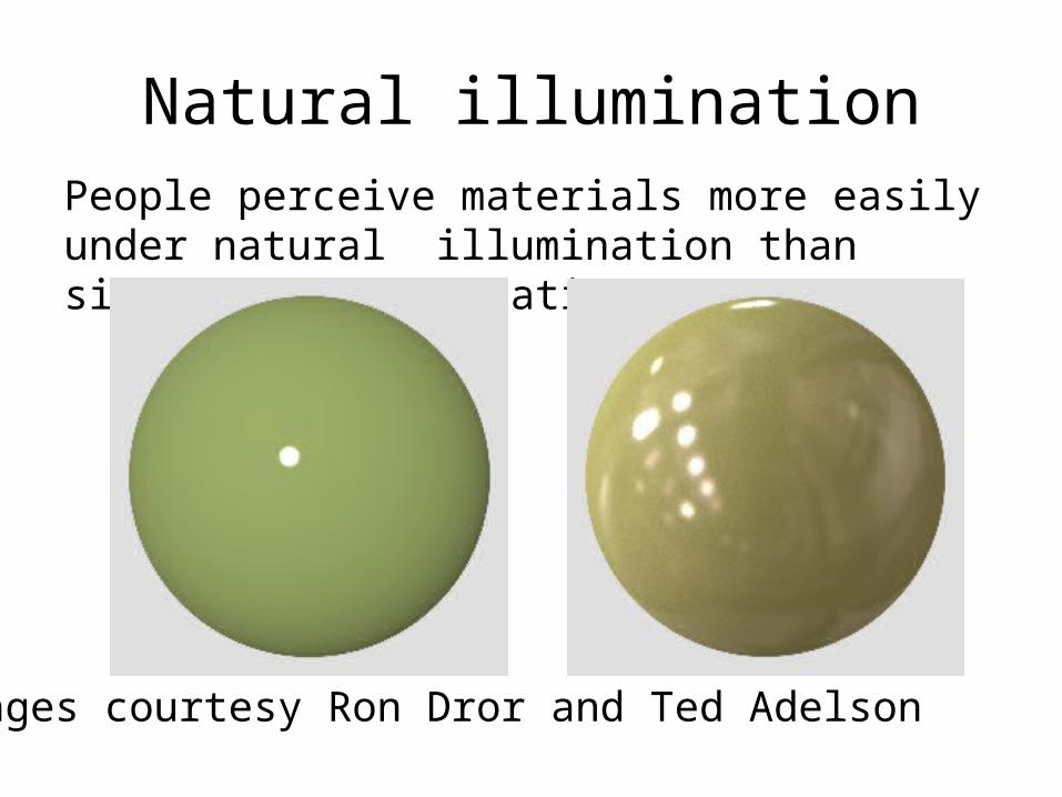
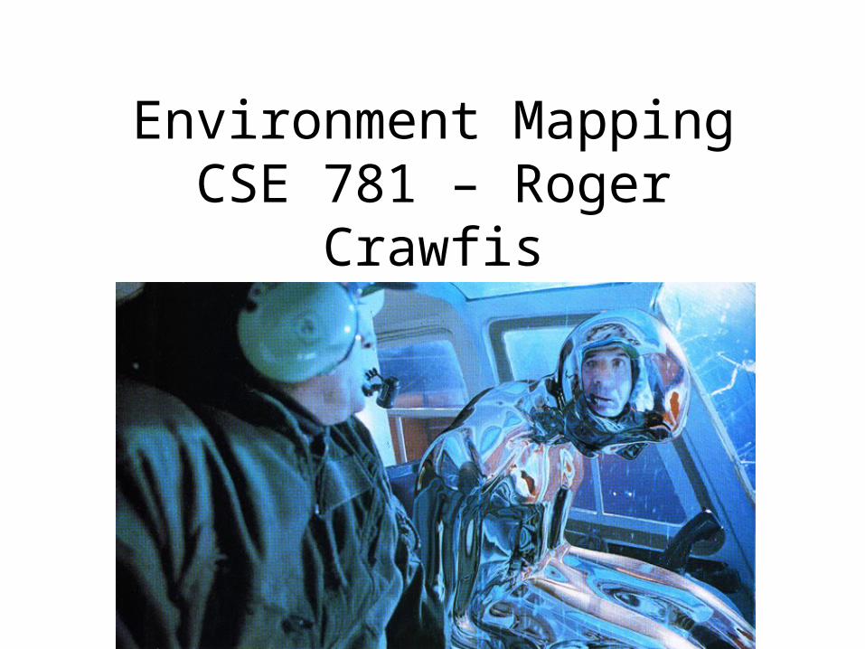
Natural illuminationPeople perceive materials more easily under natural illumination than simplified illumination.

Images courtesy Ron Dror and Ted Adelson

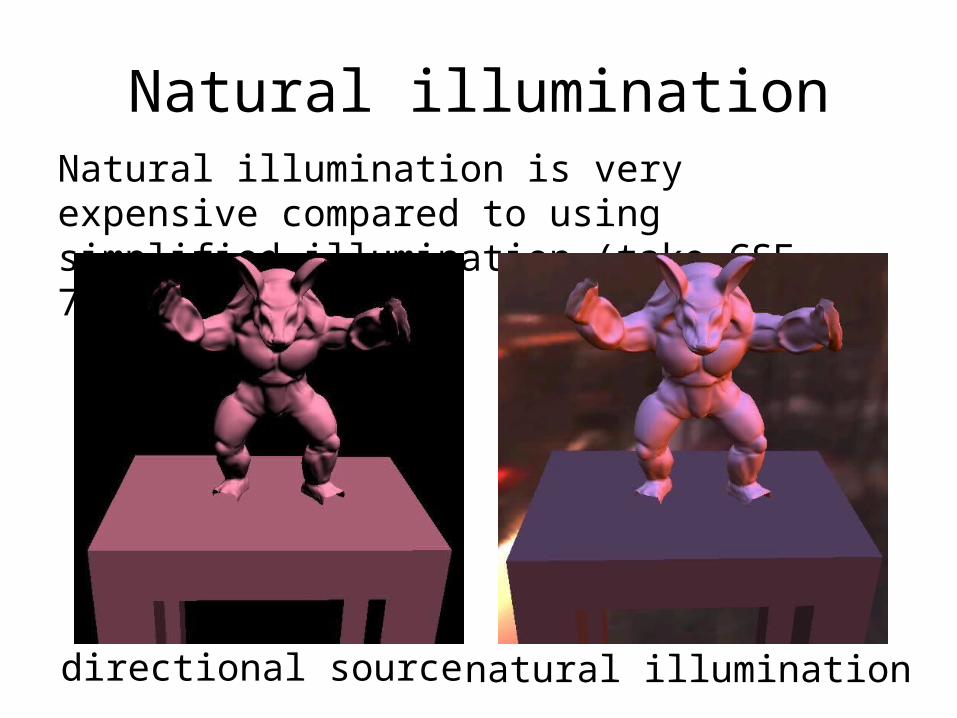
Natural illuminationNatural illumination is very expensive compared to using simplified illumination (take CSE 782).

directional source natural illumination

Environment Mapping

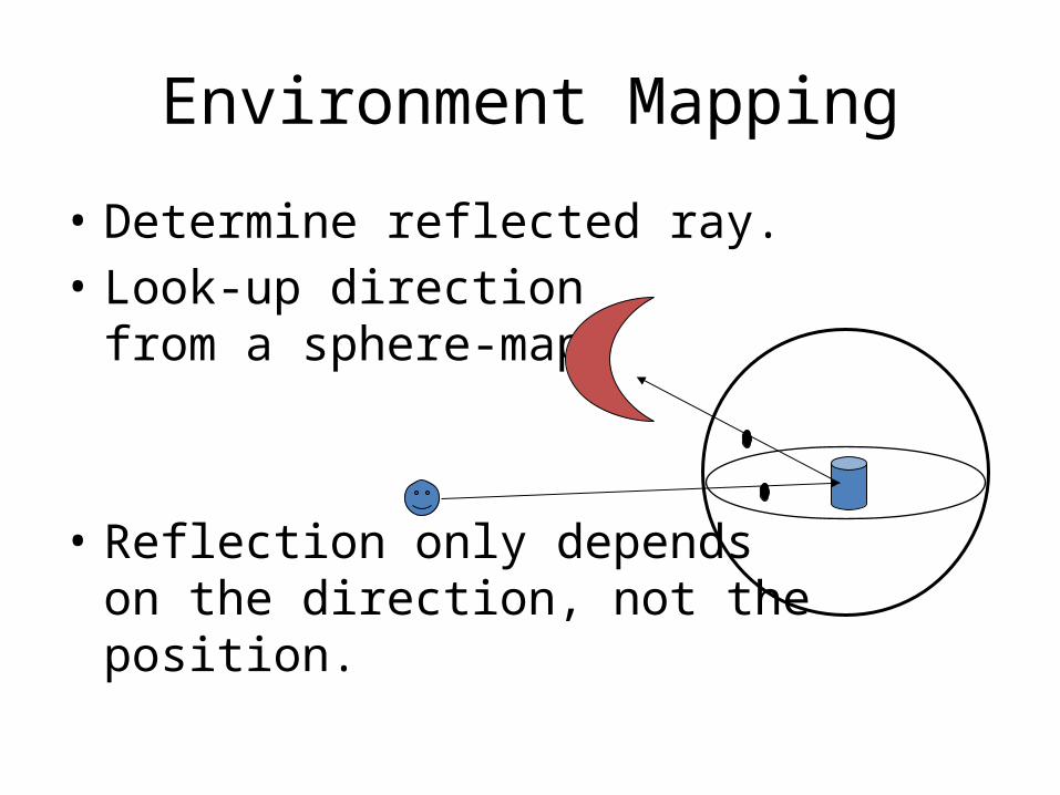
• Determine reflected ray.• Look-up direction

from a sphere-map.

• Reflection only dependson the direction, not the position.

Environment Mapping

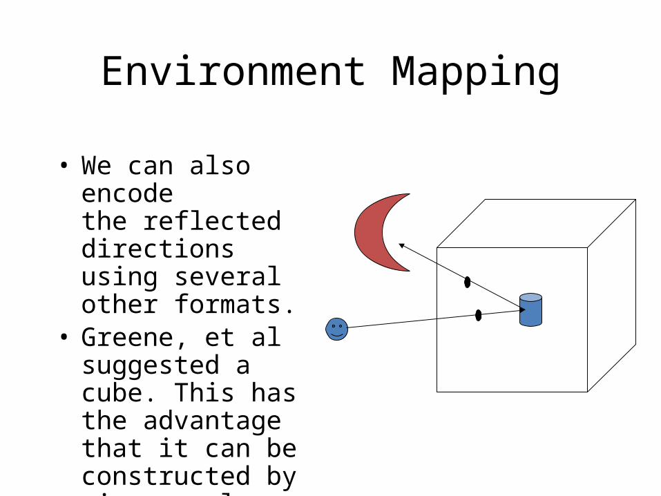
• We can also encodethe reflected directions using several other formats.

• Greene, et al suggested a cube. This has the advantage that it can be constructed by six normal renderings.

Environment Mapping

• Create six views from the shiny object’s centroid.

• When scan-converting the object, index into the appropriate view and pixel.

• Use reflection vector to index.• Largest component of reflection vector will

determine the face.

Environment Mapping

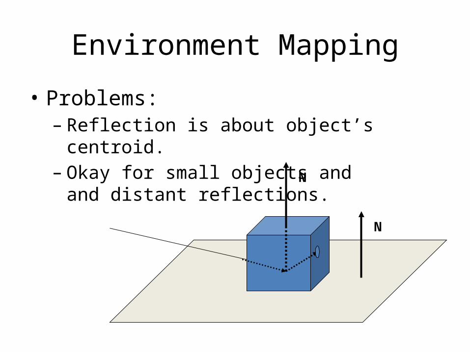
• Problems:– Reflection is about object’s centroid.– Okay for small objects and

and distant reflections. N

N

Environment Mapping

• Latitude/Longitude– Too much distortion at poles

Environment Mapping

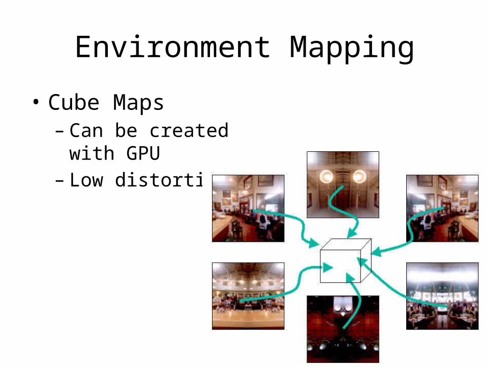
• Cube Maps– Can be created with GPU– Low distortion

Environment Mapping

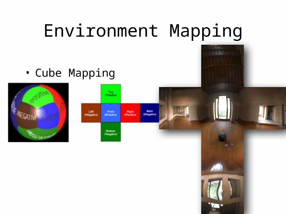
• Cube Mapping

Sphere Mapping

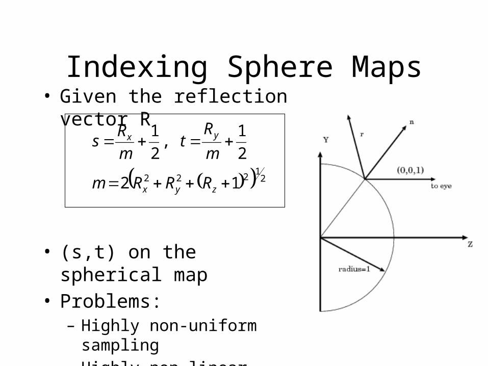
Indexing Sphere Maps• Given the reflection vector R

• (s,t) on the spherical map• Problems:

– Highly non-uniform sampling– Highly non-linear mapping

21

222 12

2

1 ,

2

1

zyx

yx

RRRm

m

Rt

m

Rs

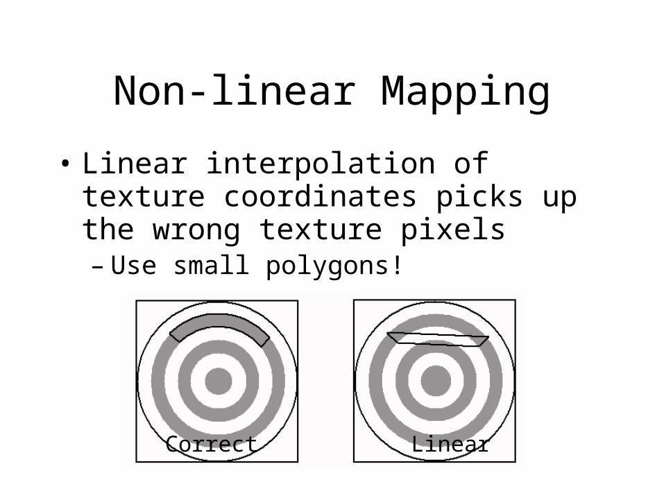
Non-linear Mapping

• Linear interpolation of texture coordinates picks up the wrong texture pixels– Use small polygons!

Correct Linear

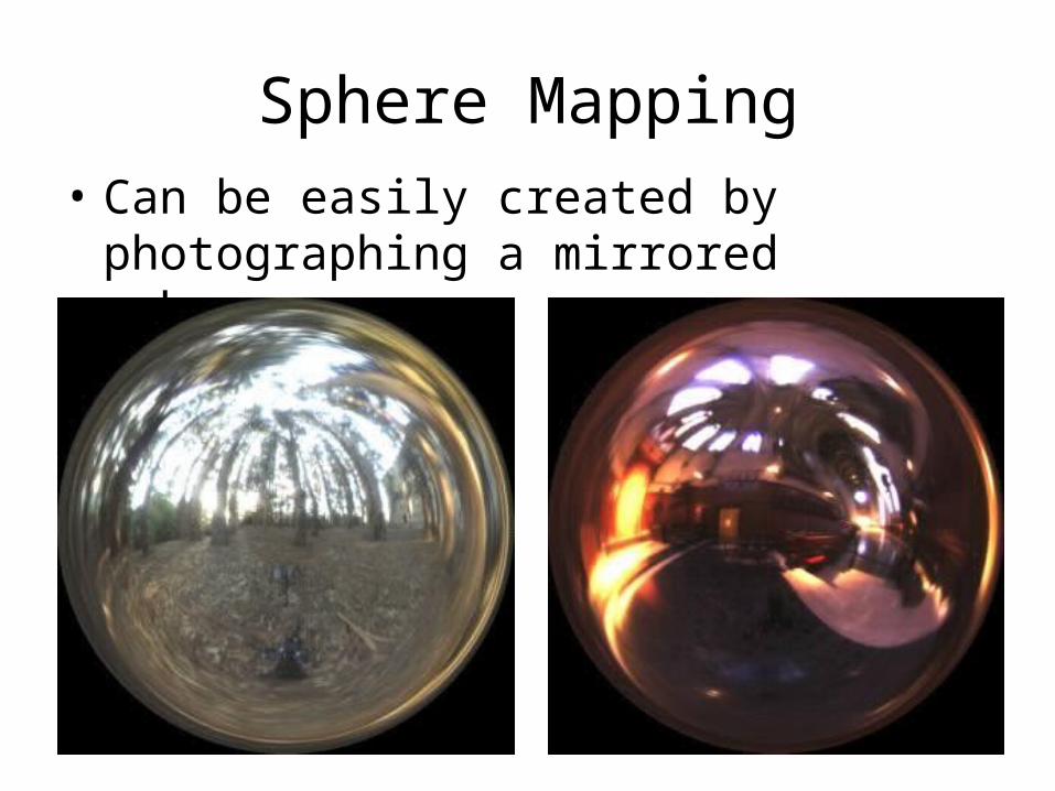
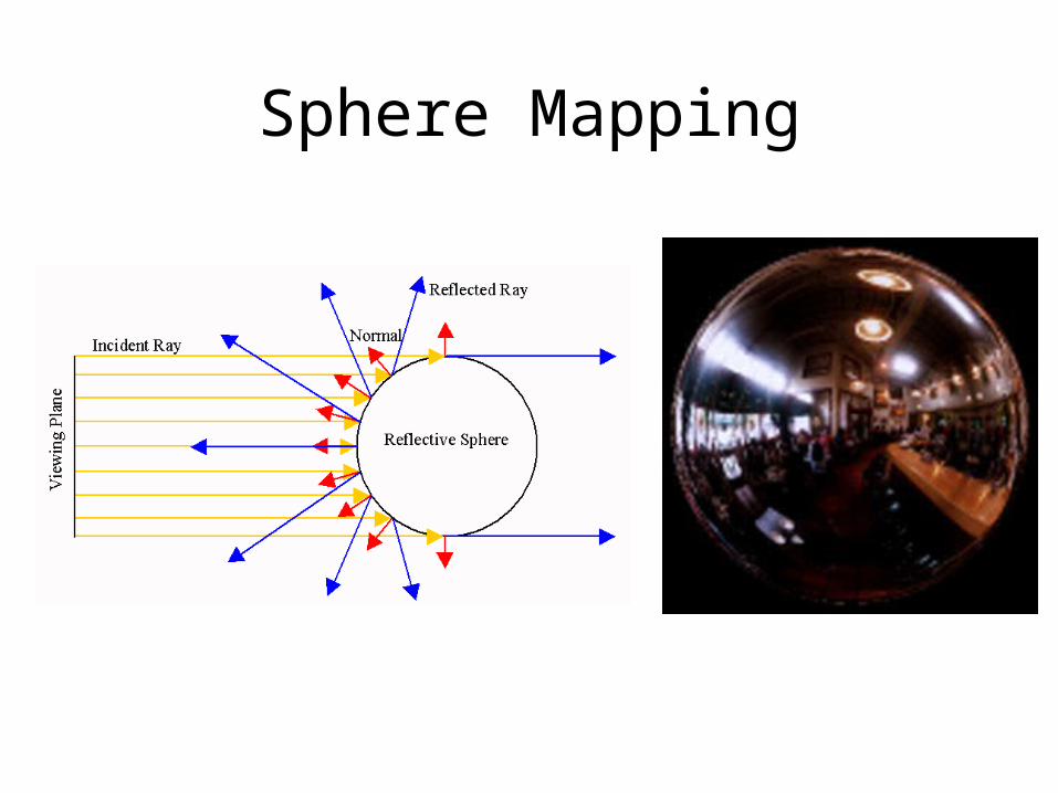
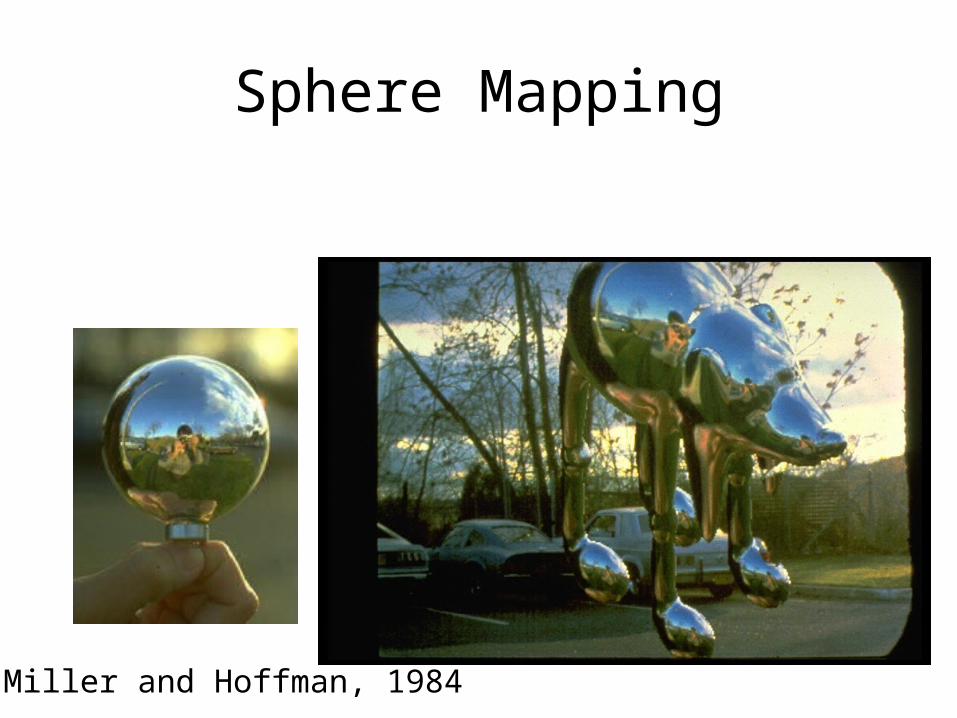
Sphere Mapping• Can be easily created by photographing a

mirrored sphere.

Sphere Mapping

Miller and Hoffman, 1984

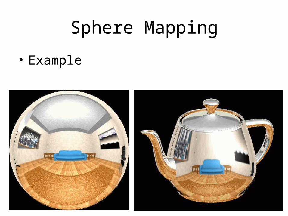
Sphere Mapping

• Example

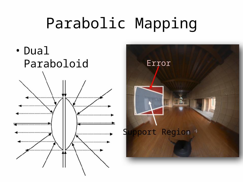
Parabolic Mapping

• Dual ParaboloidError

Support Region

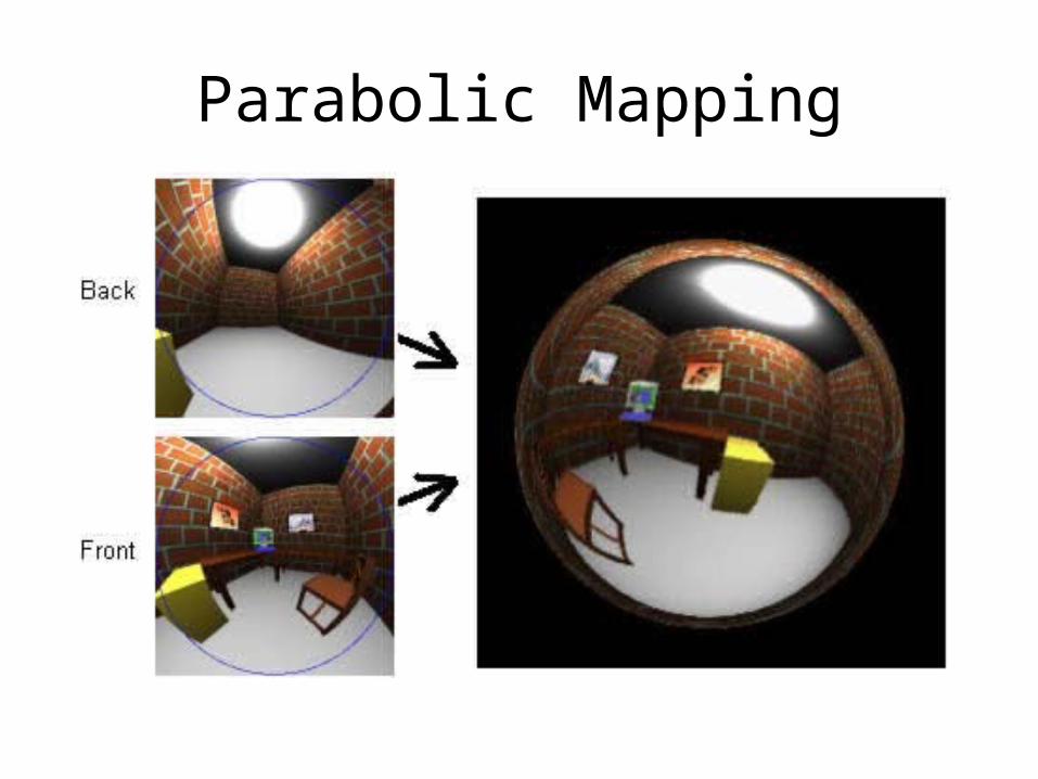
Parabolic Mapping

Environment Mapping

• Applications– Specular highlights– Multiple light sources– Reflections for shiny surfaces– Irradiance for diffuse surfaces

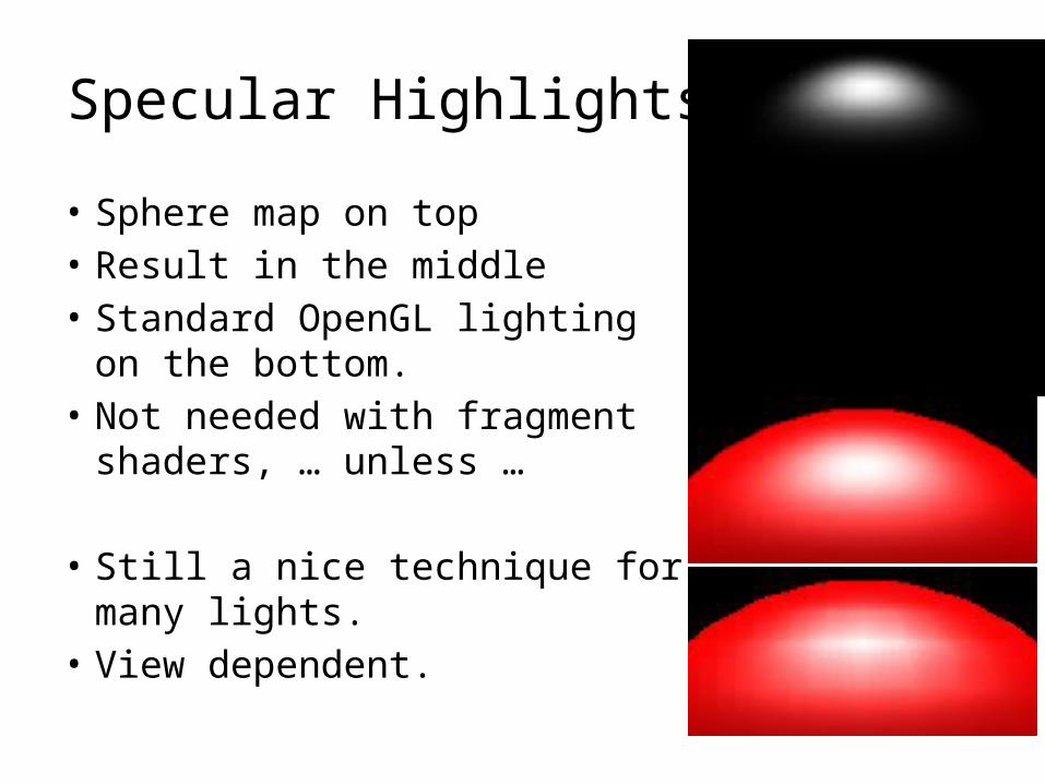
Specular Highlights

• Sphere map on top• Result in the middle• Standard OpenGL lighting on the

bottom.• Not needed with fragment shaders,

… unless …

• Still a nice technique for many lights.

• View dependent.

Chrome Mapping

• Cheap environment mapping• Material is very glossy, hence perfect

reflections are not seen.• Index into a pre-computed view independent

texture.• Reflection vectors are still view dependent.

Chrome Mapping

• Usually, we set it to a very blurred landscape image.– Brown or green on the bottom– White and blue on the top.– Normals facing up have a white/blue color– Normals facing down on average have a brownish

color.

Chrome Mapping

• Also useful for things like fire.• The major point, is that it is not important

what actually is shown in the reflection, only that it is view dependent.

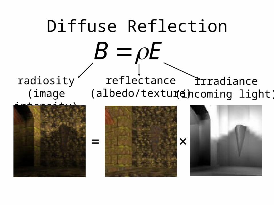
Diffuse Reflection

radiosity(image intensity)

reflectance(albedo/texture)

irradiance(incoming light)

×=

quake light map

EB

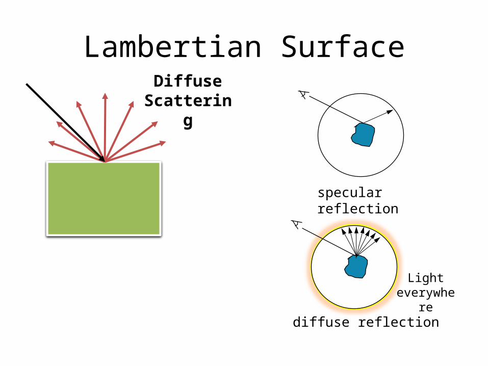
Lambertian SurfaceDiffuse

Scattering

specular reflection

diffuse reflection

Light everywhere

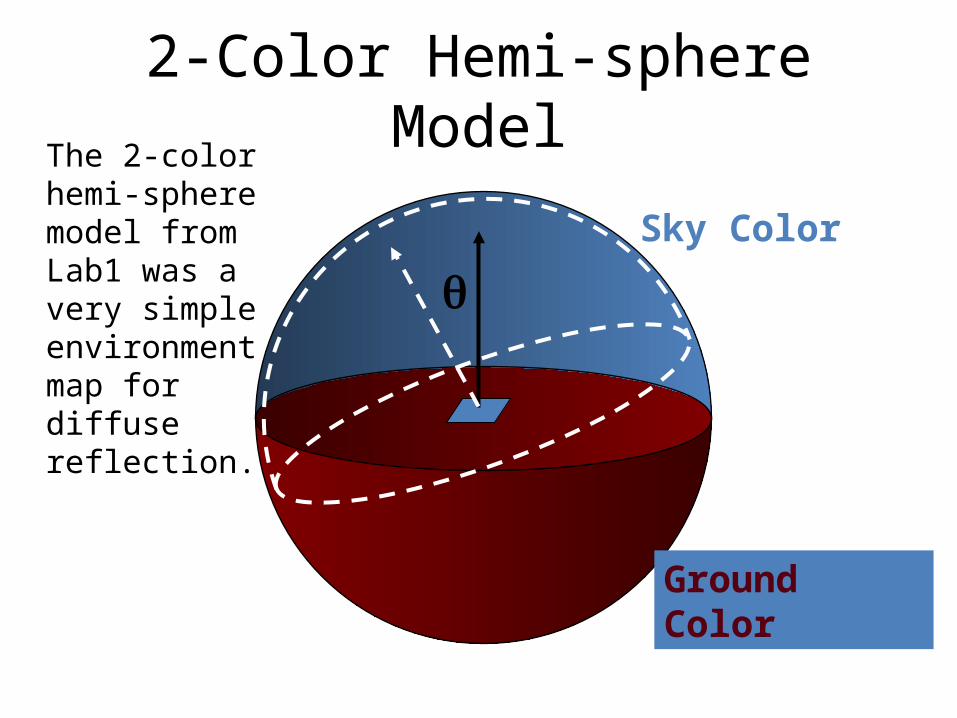
2-Color Hemi-sphere Model

Sky Color

Ground Color

q

The 2-color hemi-sphere model from Lab1 was a very simple environment map for diffuse reflection.

Model Elements

Sky Color

Final Color

Ground Color

Hemisphere Model

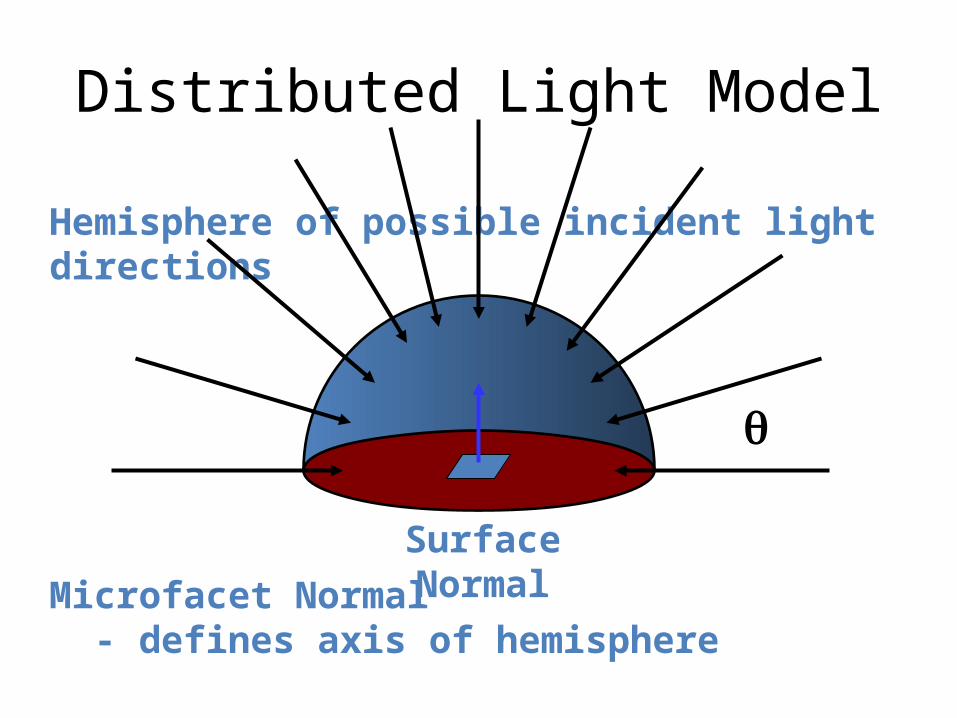
Distributed Light Model

Hemisphere of possible incident light directions

Surface Normal

Microfacet Normal - defines axis of hemisphere

q

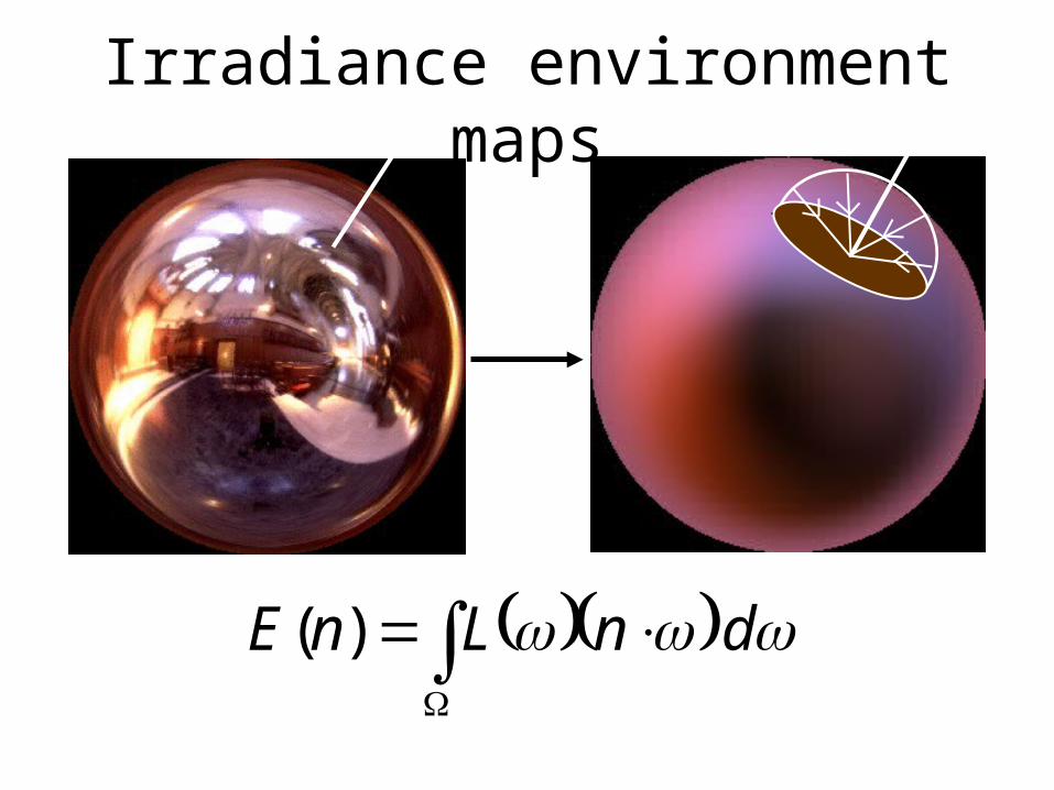
Irradiance environment maps

Illumination Environment Map Irradiance Environment Map

L n

dnLnE )(

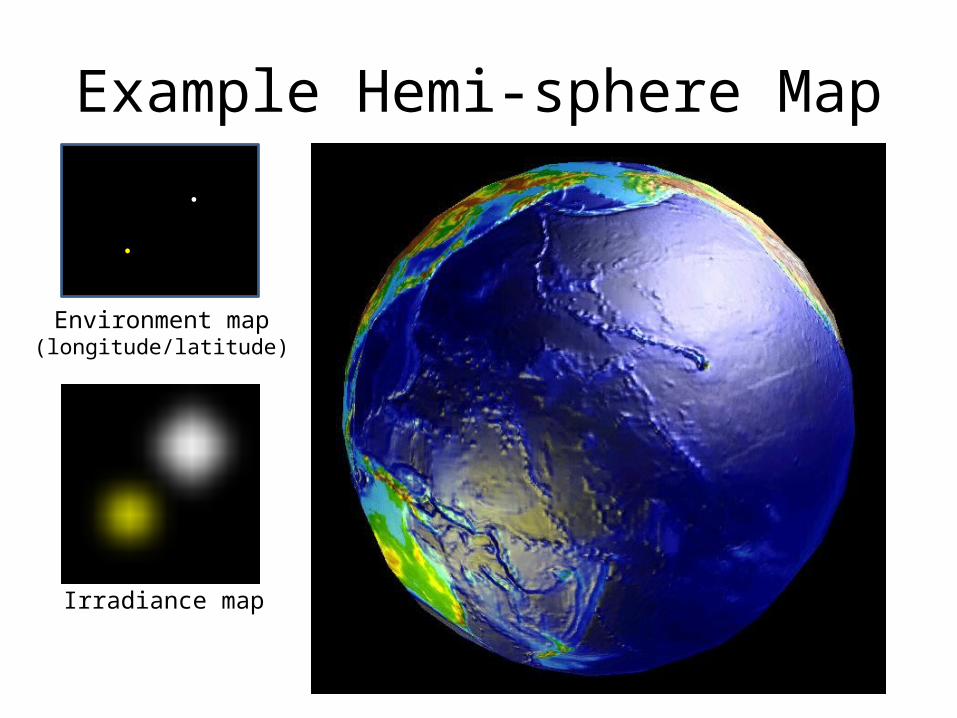
Example Hemi-sphere Map

Environment map(longitude/latitude)

Irradiance map

Cube Map And Its Integral

Spherical Harmonics

Roger CrawfisCSE 781

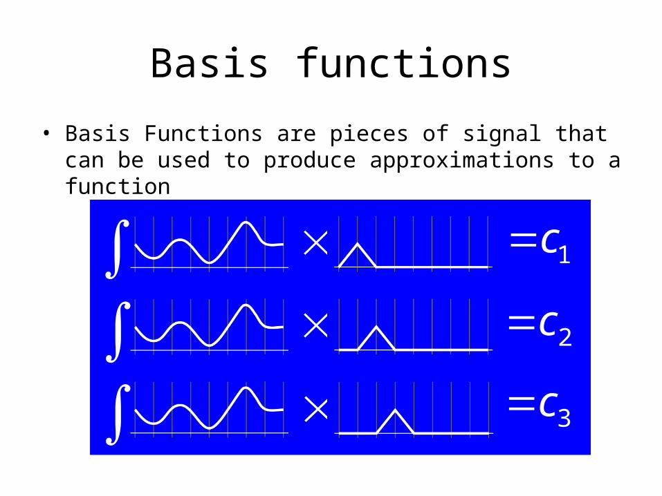
• Basis Functions are pieces of signal that can be used to produce approximations to a function

1c

2c

3c

Basis functions

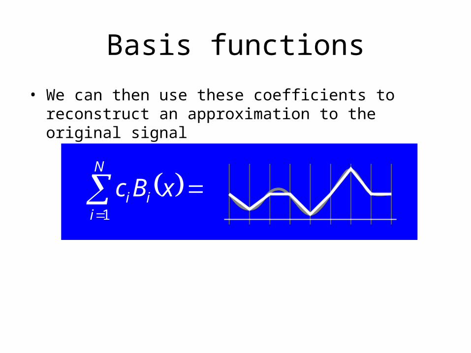
• We can then use these coefficients to reconstruct an approximation to the original signal

1c

2c

3c

Basis functions

• We can then use these coefficients to reconstruct an approximation to the original signal

xBcN

iii

1

Basis functions

Orthogonal Basis Functions

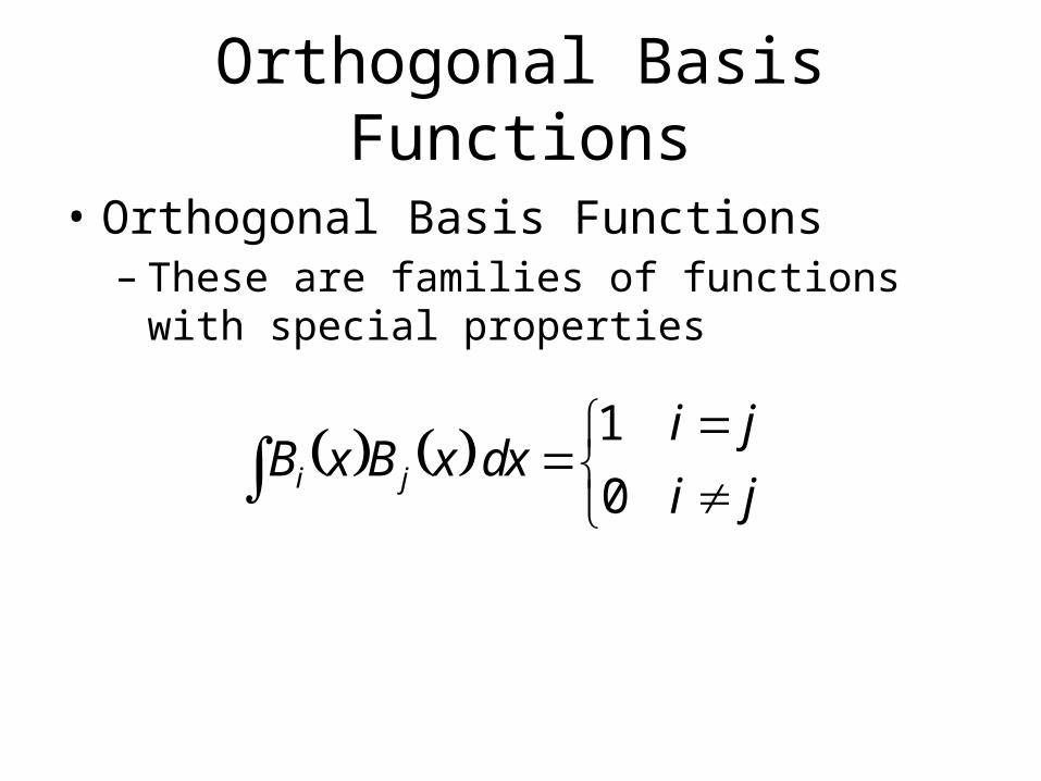
• Orthogonal Basis Functions– These are families of functions with special

properties

ji

jidxxBxB ji 0

1

Orthogonal Basis Functions

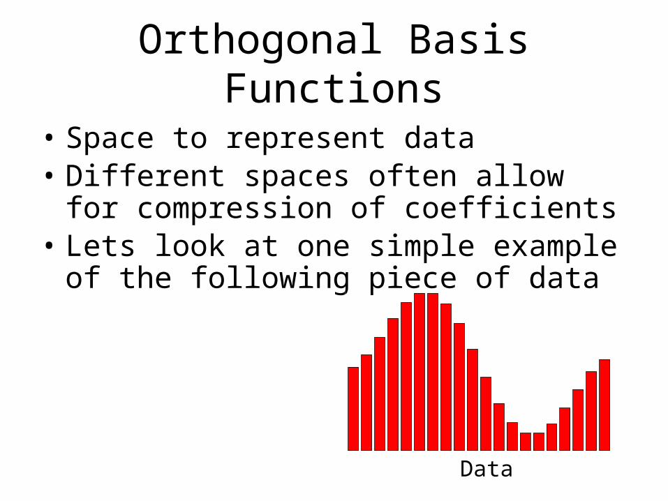
• Space to represent data• Different spaces often allow for compression

of coefficients• Lets look at one simple example of the

following piece of data

Data

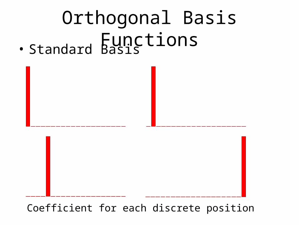
Orthogonal Basis Functions• Standard Basis

Coefficient for each discrete position

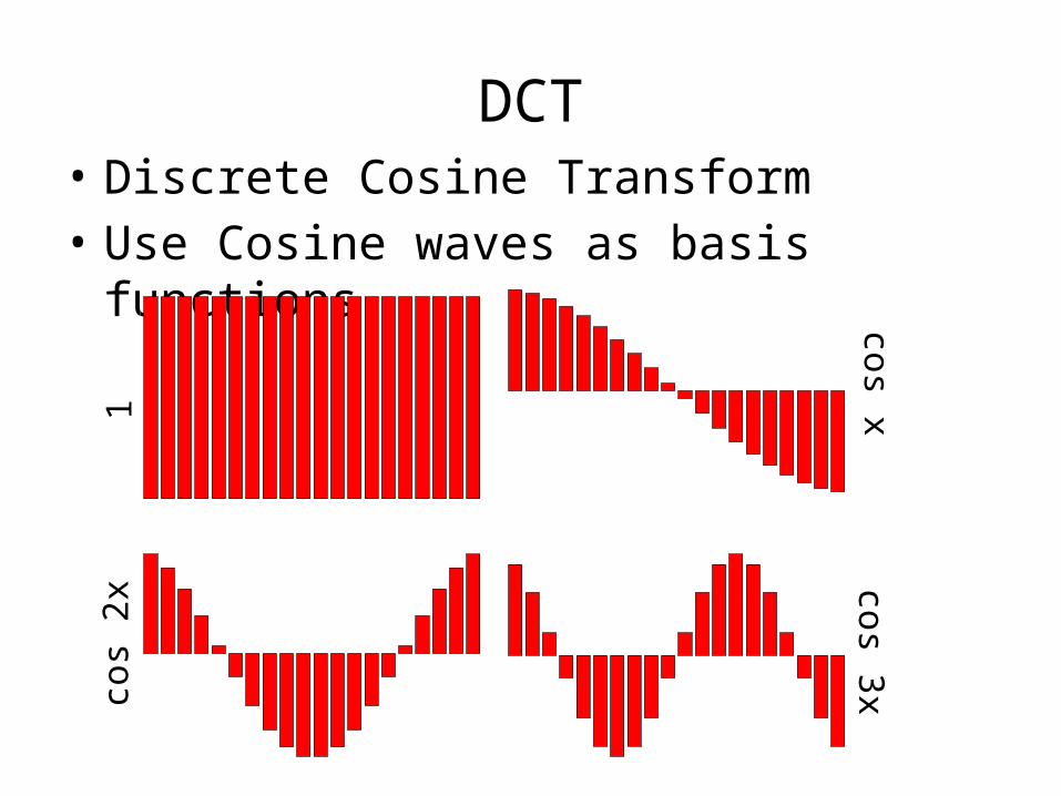
DCT• Discrete Cosine Transform• Use Cosine waves as basis functions

1

cos x

cos

2x

cos 3x

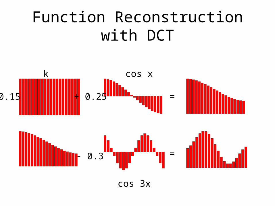
Function Reconstruction with DCT

0.15 + 0.25 =

- 0.3 =

k cos x

cos 3x

Function Reconstruction with DCT

• Only needed 3 coefficients instead of 20!– Remaining coefficients are all 0

• Most of the time data not perfect• Obtain good reconstruction from few

coefficients• Arbitrary function conversion requires

projection

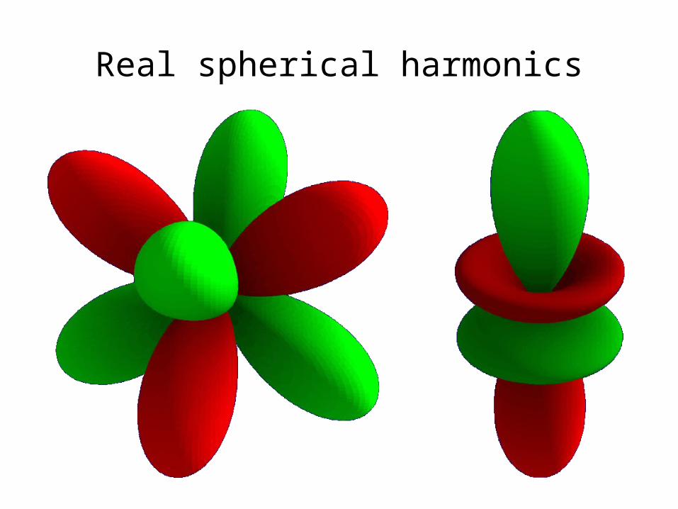
Real spherical harmonics

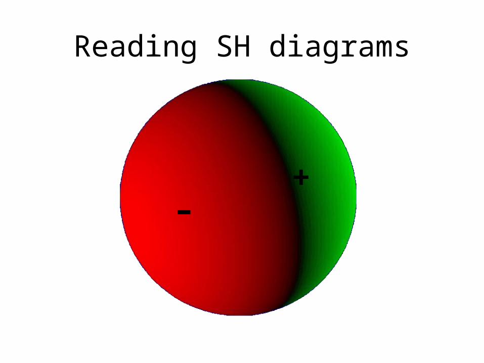
Reading SH diagrams

–+

Not thisdirection

Thisdirection

Reading SH diagrams

–+

Not thisdirection

Thisdirection

The SH functions0

0y

11y

11y

12y

22y

02y

12y2

2y

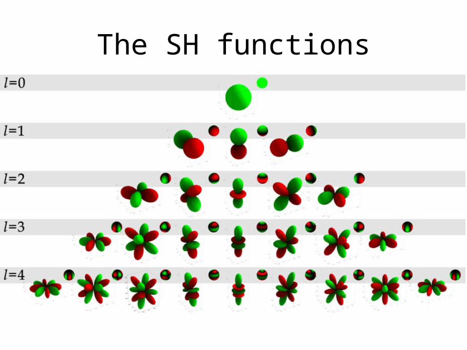
The SH functions

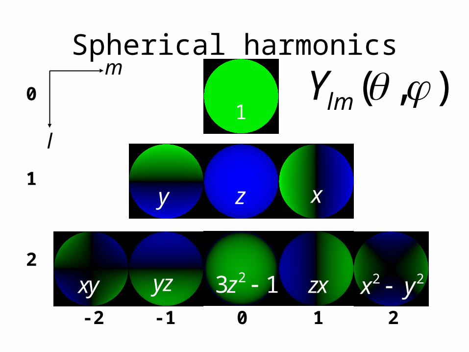
Spherical harmonics

-1-2 0 1 2

0

1

2

( , )lmY

xy z

xy yz 23 1z zx 2 2x y

1

m

l

Examples of reconstruction

Displacement mapping on the sphere

An example• Take a function comprised of two area light sources

– SH project them into 4 bands = 16 coefficients

2380042508370317000106420

27800417009400908093006790

3291

.,,.,.,.,.,.,.,,.,,.

,.,.,.,.

Low frequency light source• We reconstruct the signal

– Using only these coefficients to find a low frequency approximation to the original light source

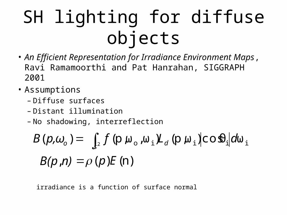
SH lighting for diffuse objects

• An Efficient Representation for Irradiance Environment Maps, Ravi Ramamoorthi and Pat Hanrahan, SIGGRAPH 2001

• Assumptions– Diffuse surfaces– Distant illumination – No shadowing, interreflection

irradiance is a function of surface normal

)( op,ωB iiiio ωθcos)ωp,()ω,ωp,(2

dLf ds)n()( Epn)B(p,

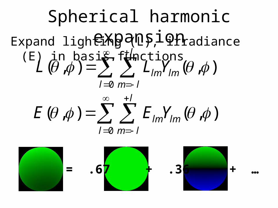
Spherical harmonic expansionExpand lighting (L), irradiance (E) in basis functions

0

( , ) ( , )l

lm lml m l

L L Y

0

( , ) ( , )l

lm lml m l

E E Y

= .67 + .36 + …

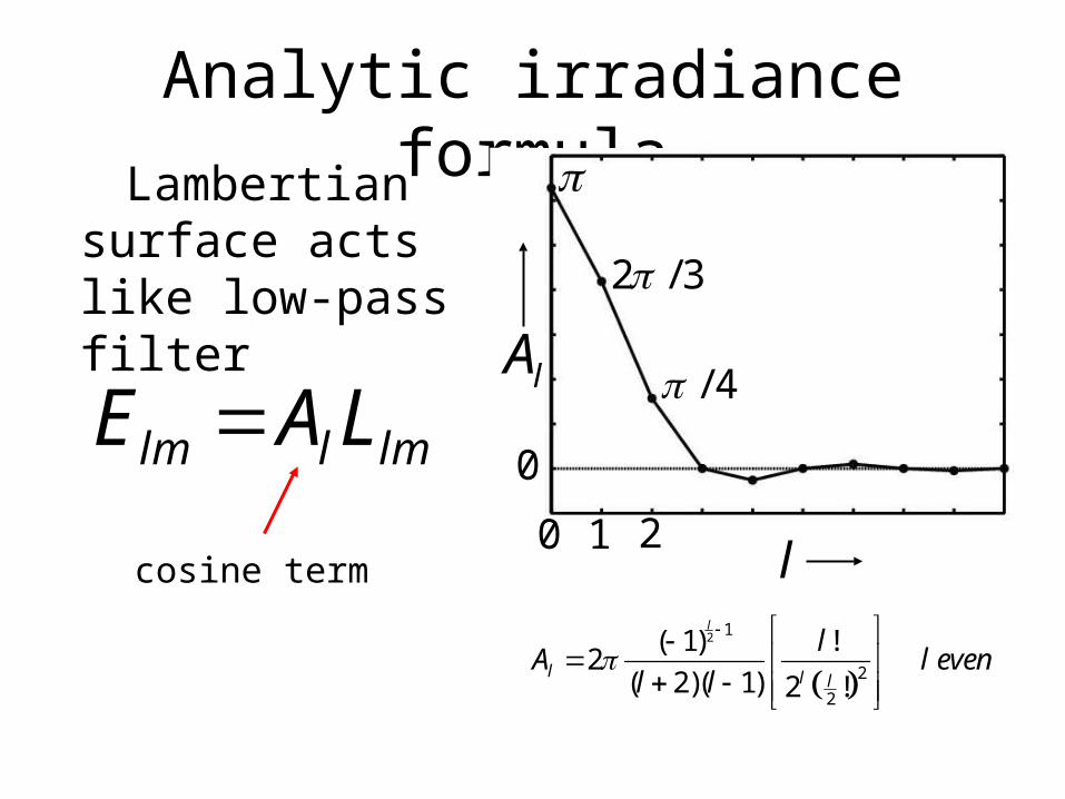
Analytic irradiance formula Lambertian surface

acts like low-pass filter

lm l lmE A LlA

2 / 3

/ 4

0

2 1

2

2

( 1) !2

( 2)( 1) 2 !

l

l l l

lA l even

l l

l0 1 2

cosine term

9 parameter approximation

Exact imageOrder 01 term

RMS error = 25 %

-1-2 0 1 2

0

1

2

( , )lmY

xy z

xy yz 23 1z zx 2 2x y

l

m

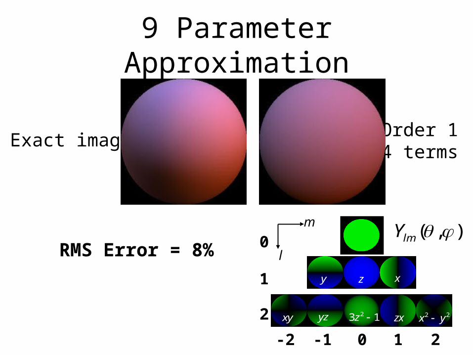
9 Parameter Approximation

Exact imageOrder 14 terms

RMS Error = 8%

-1-2 0 1 2

0

1

2

( , )lmY

xy z

xy yz 23 1z zx 2 2x y

l

m

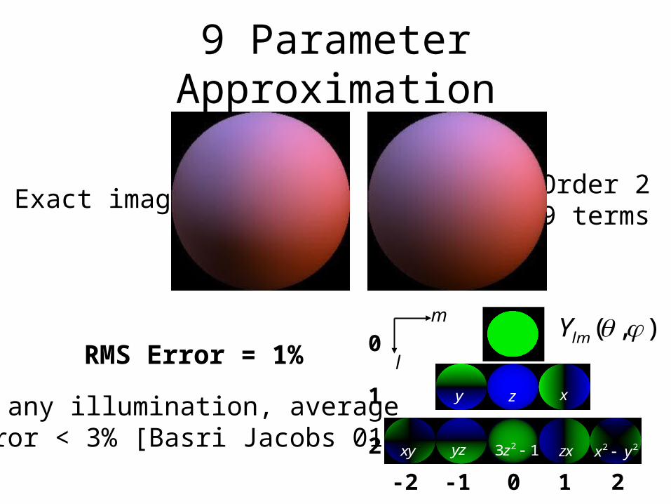
9 Parameter Approximation

Exact imageOrder 29 terms

RMS Error = 1%

For any illumination, average error < 3% [Basri Jacobs 01]

-1-2 0 1 2

0

1

2

( , )lmY

xy z

xy yz 23 1z zx 2 2x y

l

m

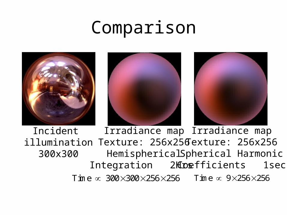
Comparison

Incident illumination

300x300

Irradiance mapTexture: 256x256

HemisphericalIntegration 2Hrs

Irradiance mapTexture: 256x256

Spherical HarmonicCoefficients 1sec

Time 300 300 256 256 Time 9 256 256

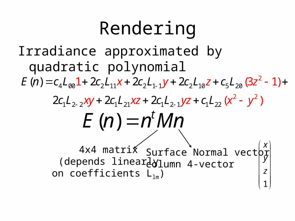
RenderingIrradiance approximated by quadratic

polynomial2

4 00 2 11 2 1 1 2 10 5 2

2 2

0

1 2 2 1 21 1 2 1 1 22

1 (3 1( ) 2 2 2

2 2 ( )2

)x y z z

x

E n c L c L c L c L c L

c L c L c Ly xz yz x yc L

( ) tE n n Mn

1

x

y

z

Surface Normal vectorcolumn 4-vector

4x4 matrix(depends linearly

on coefficients Llm)

matrix form

c1L22 c1L2-2 c1L21 c2L11

c1L2-2 -c1L22 c1L2-1 c2L1-1

c1L21 c1L2-1 c3L20 c2L10

c2L11 c2L1-1 c2L10 c4L00 –c5L20

M =

MnnnE T

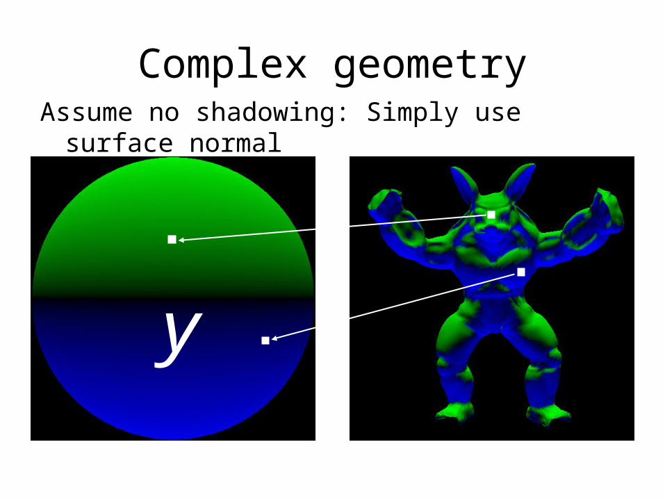
Complex geometryAssume no shadowing: Simply use surface normal

y

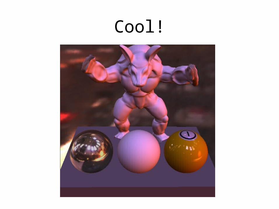
Cool!

IN4151 Introduction 3D graphics 63

Diffuse environment shading

received radiance is function of accessability

specular reflection

diffuse reflection

• Need integration over environment map

• For diffuse reflection scaled by cosinus

• Index in filtered versions of map

ambient occlusion

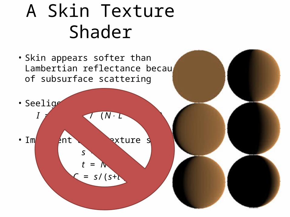
A Skin Texture Shader

• Skin appears softer than Lambertian reflectance because of subsurface scattering

• Seeliger lighting modelI = (N L) / (N L + N V )

• Implement as a texture shaders = N Lt = N V

C = s/(s+t )