Entropy–Copula in Hydrology and Climatology

AMIR AGHAKOUCHAK

Center for Hydrometeorology and Remote Sensing, Department of Civil and Environmental

Engineering, University of California, Irvine, Irvine, California

(Manuscript received 18 December 2013, in final form 11 June 2014)

ABSTRACT

The entropy theory has been widely applied in hydrology for probability inference based on incomplete

information and the principle of maximum entropy. Meanwhile, copulas have been extensively used for

multivariate analysis and modeling the dependence structure between hydrologic and climatic variables. The

underlying assumption of the principle of maximum entropy is that the entropy variables are mutually in-

dependent from each other. The principle of maximum entropy can be combined with the copula concept for

describing the probability distribution function of multiple dependent variables and their dependence

structure. Recently, efforts have beenmade to integrate the entropy and copula concepts (hereafter, entropy–

copula) in various forms to take advantage of the strengths of both methods. Combining the two concepts

provides new insight into the probability inference; however, limited studies have utilized the entropy–copula

methods in hydrology and climatology. In this paper, the currently available entropy–copula models are

reviewed and categorized into three main groups based on their model structures. Then, a simple numerical

example is used to illustrate the formulation and implementation of each type of the entropy–copula model.

The potential applications of entropy–copula models in hydrology and climatology are discussed. Finally, an

example application to flood frequency analysis is presented.

1. Introduction

Understanding the global water cycle and climatic

phenomena often requires investigating the inter-

dependence of hydrologic and climatic variables (e.g.,

drought and heat wave, flood peak and volume, and

drought severity and duration). For example, a deficit in

precipitation over a certain period of time could lead to

a deficit in soilmoisture and runoff (Kao andGovindaraju

2008). Multivariate distribution functions have been

widely used in the literature for modeling two or more

dependent hydrological variables and their dependence

structure (Salvadori and De Michele 2007; Hao and

AghaKouchak 2013; Nazemi and Elshorbagy 2012). A

number of methods to construct a joint distribution have

been proposed and applied, including the kernel density

estimation, entropy method, and copulas, to name a few

(Kapur 1989;Kotz et al. 2000;Grimaldi and Serinaldi 2006;

Nelsen 2006; Serinaldi and Grimaldi 2007; Balakrishnan

and Lai 2009; AghaKouchak et al. 2010a,b).

In the past decade, application of copulas in hydrology

has grown rapidly, owing to the fact that using copulas

were efficient for describing the dependence among

multiple hydrologic variables (Salvadori and DeMichele

2007; Favre et al. 2004). The copula theory offers a flexi-

bleway to construct a joint distribution independent from

the marginal distributions (Sklar 1959). Copulas are used

primarily to model the dependence structure between

two or more variables [e.g., precipitation and soil mois-

ture (Hao and AghaKouchak 2014) or flood peak and

volume (Salvadori et al. 2007)]. A variety of copula

families have been developed and can be used to model

different dependence structures (Joe 1997; Trivedi and

Zimmer 2005; Nelsen 2006). The main advantage of this

approach is that construction of a joint distribution

through a copula is independent of the marginal distri-

butions of the individual variables. For an introduction to

the copula theory, the reader is directed to Joe (1997) and

Nelsen (2006). A detailed review of the development and

applications of copulas in hydrology is provided inGenest

and Favre (2007) and Salvadori and De Michele (2007).

Denotes Open Access content.

Corresponding author address: Amir AghaKouchak, E/4130 En-

gineeringGateway,University ofCalifornia, Irvine, Irvine, CA92617.

E-mail: amir.a@uci.edu

2176 JOURNAL OF HYDROMETEOROLOGY VOLUME 15

DOI: 10.1175/JHM-D-13-0207.1

� 2014 American Meteorological Society

Univariate and multivariate statistical analysis in hy-

drology and climatology typically involves inference of

probability distribution, for example, flood frequency

analysis, rainfall simulation, extreme value analysis, and

geostatistical interpolation (Singh 1992; Stedinger 1993;

Bárdossy 2006). A univariate (multivariate) probability

distribution assigns probabilities to univariate (multi-

variate) hydrologic or climatic events. If there is no

reason for one event to occur more frequently than

other events, then the probabilities of all events will be

equal. This is known as the principle of insufficient

reason (Singh 2011). However, if there is some knowl-

edge or partial information on the nonuniformity of the

events (or outcomes of a certain process), the principle

of maximum entropy allows for the inclusion of the

available information in assignment of probabilities to

different events or outcomes of a process (Singh 2011).

In other words, the principle of maximum entropy offers

a methodology for deriving a probability distribution

from limited information (Zhao and Lin 2011). The

entropy theory was first formulated by Shannon (1948) as

a measure of information (or uncertainty). The principle

of maximum entropy was developed for probability in-

ference on the basis of partial information, given a set

of constraints (Jaynes 1957a,b). The approach leads to

a target distribution with the maximum entropy that sat-

isfies a set of constraints. Entropy offers the opportunity

to account for more moments, beyond just the second

moment, which describes the deviation around the mean

(Zhao and Lin 2011). The concept of maximum entropy

for probability density inference has been applied exten-

sively in a variety of areas, including physics, chemistry,

economics, and hydrology (Kapur 1989; Kesavan and

Kapur 1992; Brunsell 2010; Hao and Singh 2013). For

a comprehensive review of the development and appli-

cations of the entropy theory in hydrology, the interested

reader is referred to Singh (1997) and Singh (2011).

The underlying assumption of the principle of maxi-

mum entropy is that the entropy variables are mutually

independent from each other (Jaynes 1957a). Copulas,

on the other hand, are used to describe the dependence

between multiple variables. Consequently, the principle

of entropy can be combined with the concept of copula

to handle mutually dependent variables (i.e., describing

probability distribution function of multiple dependent

variables and their dependence structure). Recently,

efforts have been made to integrate the entropy and

copula concepts (hereafter, entropy–copula) in various

forms to take advantage of the strengths of both

methods. Two important properties of a copula density

function are uniformly distributed margins and a de-

pendence structure that describes the degree of associ-

ation between the margins. With these properties as the

partial knowledge of a target copula, new copulas can be

derived based on the entropy theory. The most common

approach to derive an entropy–copula method is to

maximize the entropy of the copula density function

using the two properties as constraints (in discrete,

continuous, or mixed forms) (Chu and Satchell 2005;

Dempster et al. 2007; Piantadosi et al. 2007; Pougaza

et al. 2010; Chu 2011; Pougaza and Mohammad-Djafari

2011; Ané and Kharoubi 2003; Piantadosi et al. 2012a,b;Pougaza and Mohammad-Djafari 2012; Hao and Singh

2012). The entropy–copula methods generally retain the

advantage of the commonly used parametric copula: the

joint distribution construction will be independent of

the marginal distributions. While the entropy–copula

methods seem to be powerful and promising techniques,

few studies have utilized them formodeling hydrological

and climatic variables.

In this study, the recently developed entropy–copula

methods are reviewed in detail. The currently available

models are then categorized into three main groups based

on their model structures. Then, a simple numerical exam-

ple is used to illustrate the formulation and implementation

of each type of the entropy–copula model. A discussion of

broader potential applications in hydrology and climatology

is provided, followed by an example application of the en-

tropy–copula concept to flood frequency analysis.

The remainder of this paper is outlined as follows. The

entropy and copula concepts are introduced in sections 2

and 3, respectively. The recently developed entropy–

copulamethods are reviewed and categorized in section 4,

followed by a numerical example in section 5. Section 6

provides a discussion on the potential applications to hy-

drology and climatology and an example application to

flood frequency analysis. The last section summarizes the

results and conclusions.

2. Entropy theory

For a random variable X with probability density func-

tion (PDF) f(x) defined on the interval [a, b], the Shannon

entropy can be defined as (Shannon 1948; Jaynes 1957a,b)

H152

ðbaf (x) lnf (x) dx . (1)

The maximum entropy concept consists of inferring the

probability distribution that maximizes information

entropy given a set of constraints. For the realizations xi(i 5 1, 2, . . . , n) of the random variable X, the general

form of the constraints can be expressed as (Kapur 1989)ðbagr(x)f (x) dx5 gr(x) r5 0, 1, 2, . . . ,m , (2)

DECEMBER 2014 AGHAKOUCHAK 2177

where gr(x) denotes a function of x, with gr(x) being the

expectation of gr(x). In this equation,m is the number of

constraints, and the rth expected value of gr(x) can be

obtained from observations (e.g., mean and variance;

see Singh 2011). For r5 0, the constraint given in Eq. (2)

can be described as ðbaf (x) dx5 1. (3)

This constraint indicates that the PDF must satisfy the

so-called total probability theorem, also termed as the

normalization condition. In other words, this con-

straint ensures that the integration of the PDF f(x)

over the entire interval equates unity. While there

may be a variety of distributions that satisfy the above

constraints shown in Eq. (2), according to the principle

of maximum entropy, the most suitable distribution

function is the one that leads to the maximum entropy

(Jaynes 1957a). The maximum entropy PDF can be

obtained by maximizing the entropy in Eq. (1) subject

to Eq. (2) with the Lagrange multipliers method as

(Kapur 1989)

f (x)5 exp[2l02 l1g1(x)2 l2g2(x) � � �2 lmgm(x)] ,

(4)

where li, i5 0, 1, 2, are the Lagrangemultipliers that can

be estimated with the Newton–Raphson algorithm

(Kapur 1989). The Lagrange multipliers method allows

maximizing (or minimizing) a function subject to some

constraints (Vapnyarskii 2001). By integrating Eq. (4),

one can obtain the cumulative distribution function

(CDF).

Kullback and Leibler (1951) developed the principle

of minimum cross (or relative) entropy as a way to infer

the probability based on the prior information. Suppose

that q(x) is an unknown density and p(x) is the prior

estimate of q(x). The cross entropyH2 can be defined as

H25

ðbaq(x) ln[q(x)/p(x)] dx . (5)

Minimizing the cross entropy in Eq. (5) subject to the

constraints in Eq. (2) yields (Kapur 1989)

q(x)5 p(x) exp[2 l02 l1g1(x)2 l2g2(x) � � �2lmgm(x)] .

(6)

The minimum cross entropy measures the distance of

one distribution to another. When the prior distribution

p(x) is the uniform distribution, the minimum cross-

entropy distribution q(x) reduces to the maximum en-

tropy distribution shown in Eq. (4).

3. Copula theory

The copula theory has been commonly used to con-

struct the joint distribution of multiple variables. For the

bivariate case, denote the marginal distributions for the

continuous random variablesX and Y as F(x) (orU) and

G(y) (or V), respectively. The joint CDFs C(u, y) or

F(x, y) can be constructed with the copula C in the form

(Sklar 1959)

F(x, y)5C[F(x),G(y)]5C(u, y) . (7)

The copula C links the marginal distributions by map-

ping the two univariate marginal distributions into

a joint distribution. If the marginal distribution is con-

tinuous, the copula function is unique. The copula

functionC(u, y) is a function from [0, 1]2 to [0, 1] with the

following properties (Nelsen 2006):

C(u, 0)5C(0, y)5 0 C(u, 1)5C(1, y)5 1. (8)

For u1, u2, y1, and y2 in [0, 1], such that u1# u2 and y1# y2,

C(u2, y2)2C(y2, y1)2C(u1, y2)1C(u1, y1)$ 0. (9)

Having the copula distribution C(u, y), the copula den-

sity function c(u, y) can be defined as (Nelsen 2006):

c(u, y)5 ›C2(u, y)/›u›y . (10)

4. Entropy–copula models

In this paper, the currently available entropy–copula

models are broadly classified into three groups based on

their model structures: 1) continuous maximum entropy

copula (CMEC), 2) mixed maximum entropy copula

(MMEC), and 3) discrete density maximum entropy

copula (DDMEC). In this section, three recently de-

veloped entropy–copula methods (one from each cate-

gory) are reviewed in depth. For the sake of simplicity, the

formulations of the entropy–copula method for deriving

the copula density function are introduced in the bivariate

case [i.e., c(u, y)]; however, extension of the presented

equations to higher dimensions is straightforward (see

Piantadosi et al. 2012b; Hao and Singh 2013).

a. CMEC

Themost entropic canonical copula (MECC) is derived

by maximizing the entropy of the copula density function

c(u, y) subject to constraints in the form of continuous

functions of marginal probabilities (U and V; Chu and

Satchell 2005; Chu 2011). TheMECC is also termed as the

empirical copula in Chui and Wu (2009). The constraints

to derive the copula are imposed through a continuous

2178 JOURNAL OF HYDROMETEOROLOGY VOLUME 15

function of the marginal, and thus, this method is termed

as the continuous maximum entropy copula. The entropy

of the copula density function c(u, y) can be expressed as

W52

ð10

ð10c(u, y) lnc(u, y) du dy . (11)

The condition that the integration of the copula density

function c(u, y) over the space [0, 1]2 equates unity can

be satisfied by specifying the following constraint:

ð10

ð10c(u, y) du dy5 1. (12)

The condition that the marginal probability is uniformly

distributed on [0, 1] can be fulfilled by specifying the

following constraint:ðu0

ð10c(x, y) du dy5 u

ð10

ðy0c(u, y) du dy5 y . (13)

The joint behavior (or dependence structure) of the

marginal probability U and V can be modeled by spec-

ifying the constraint asð10

ð10h(u, y)c(u, y) du dy5E[h(u, y)] , (14)

where h(u, y) is a function of the marginal u and y, which

can be related to a certain dependence structure, and

E[h(u, y)] is the expectation of the function h(u, y). There

are several dependence measures that can be linked to Eq.

(14) (Chu 2011). For example, when h(u, y) 5 uy, E[h(u,

y)] can be expressed as a linear form of the Spearman rank

correlation coefficient (r), which is a nonparametric sta-

tistical dependence measure:

ð10

ð10uyc(u, y) du dy5

r1 3

12. (15)

The Spearman rank correlation coefficient assesses the

degree of association between two variables and depends

solely on the choice of copula and not the marginal dis-

tribution of the underlying variables (Joe 1997). The

problem of inferring the copula density function c(u, y)

can then be formalized as maximizing the entropy subject

to the constraints given in Eqs. (12)–(14). However, there

are infinite combinations of constraints (continuums of

integrals of continuous random variables) in Eq. (13), thus

making it difficult to solve the optimization problem of

maximizing the entropy. An alternative method is to use

Carleman’s condition to transform these constraints into

the moment constraints (Durrett 2005; Chu 2011). In this

approach, the constraints in Eq. (13) can be replaced as

ð10

ð10urc(u, y) du dy5

1

r1 1

ð10

ð10yrc(u, y) du dy5

1

r1 1,

(16)

where r5 1, 2, . . . ,m, andm is themaximumorder of the

moment. Denote the constraints as gk(u, y) 5 [u, . . . , ur,

y, . . . , yr, h(u, y)], k 5 1, . . . , N, where N is the number

of constraints. The copula density function c(u, y) can

then be derived by maximizing the entropy in Eq. (11),

subject to the constraints in Eqs. (12), (14), and (16) as

(Chu 2011)

c(u, y)5 exp[2l02 lkgk(u, y)]

5 exp

�2l02 �

m

r51

(lrur 1 gry

r)2 th(u, y)

�, (17)

where l1, . . . , lm; g1, . . . , gm; and t are the parameters

and l0 can be expressed as

l0 5 ln

�ð10

ð10exp

�2�

m

r51

(lrur 1 gry

r)2 th(u, y)

�du dy

�.

(18)

It has been shown that the model parameters can be esti-

mated through minimizing a convex function G expressed

as (Mead and Papanicolaou 1984; Kapur 1989)

G5 l01 �m

k51

lkgk . (19)

There is no analytical solution to the above optimization

(minimization) problem, and hence, a numerical method

such as the Newton–Raphson iteration can be used to

estimate the parameters.

Similar concepts have been applied to derive a mul-

tivariate distribution from the entropy theory based on

moments of the data (Zhu et al. 1997; Phillips et al.

2006; Hao and Singh 2011). An essential procedure in

implementing the maximum entropy distribution is

selecting appropriate constraints to avoid/control over-

fitting (Phillips et al. 2006).

b. MMEC

Instead of matching the moments of the marginal dis-

tribution, the constraints can be specified as the cumu-

lative probability at a set of points to satisfy the uniformly

distributedmarginal (Dempster et al. 2007; Friedman and

Huang 2010). This type of model is categorized as the

mixed maximum entropy copula in this study. The so-

called relative entropy copula (REC), proposed by

Dempster et al. (2007), belongs to this category. The

REC allows for the driving of a copula family by mini-

mizing the entropy relative to a specific copula subject to

DECEMBER 2014 AGHAKOUCHAK 2179

a set of constraints. In this method, the issue of infinite

constraints in Eq. (13) is addressed by selecting a finite

number of points pi and qj, where i, j5 1, 2, . . . ,N, and by

conditioning the constraints to only hold for those points,

but not for all, within the interval [0, 1] (Dempster et al.

2007). Thus, the constraints inEq. (13) can be replacedwithðpk

pk21

ð10c(u, y) du dy5 pk 2 pk21 (20)

and

ð10

ðqk

qk21

c(u, y) du dy5 qk 2qk21 k5 1, 2, . . . ,N ,

(21)

where 0# p0. . . .# pk. . .# pN#1 and 0# q0. . . .# qk. . .#

qN #1 are a set of sequences of marginal probabilities at

discrete points. Various functions of the marginal distri-

butions can be used to model data properties (e.g., de-

pendence structure). Here, the pairwise product of the

marginal in Eq. (15) (the Spearman rank correlation co-

efficient) can be used as the constraint to derive theREC.

Assuming the prior copula to be p(u, y), the relative

entropy of the copula density function c(u, y) can be

expressed as

W5

ð10

ð10c(u, y) ln

c(u, y)

p(u, y)du dy . (22)

The REC can be obtained by minimizing the relative

entropy in Eq. (22), subject to the constraints given in

Eqs. (20), (21), and (15) as

c(u, y)5p(u, y) exp

(2l02 �

N

k51

[akI(pk # u# pk11)]

2 �N

k51

[bkI(qk# y# qk11)]2 luy

), (23)

where I is the indicator function; ak, bk, k 5 1, 2, . . . , N,

and l are unknown parameters to be estimated; and l0 can

be expressed as a function of the unknown parameters

l05 ln

ð10

ð10p(u, y) exp

(2 �

N

k51

[akI(pk # u# pk11)]

2 �N

k51

[bkI(qk# y# qk11)]2 luy

)du dy .

(24)

The parameters can be estimated using the procedure

discussed in section 4a. The REC enables incorporation

of a prior distribution, which can be a prior choice of

target copula, to derive the target copula density func-

tion (Dempster et al. 2007). Theoretically, this prior

copula can also be introduced within the framework of

the MECC by minimizing the relative entropy with re-

spect to the choice of prior copula.

c. DDMEC

The uniformly distributedmarginal property and certain

types of dependence structures can be approximated by

discrete forms of constraints to derive a copula with max-

imum entropy. These types of entropy–copula models are

classified as the discrete density maximum entropy copula.

The recently proposed maximum entropy checkerboard

copula (MECBC), for example, belongs to this category

(Piantadosi et al. 2007, 2012a,b). A d-dimensional check-

erboard copula is a distribution with the density function

defined by a step function on a d-uniform subdivision of

the hypercube [0, 1]d that uniformly approximates a con-

tinuous copula (Piantadosi et al. 2012b). In addition, the

grade correlation is imposed as a constraint to preserve the

dependence structure in the original data. For the bivariate

case, a two-dimensional checkerboard copula can be con-

structed, with n equal subintervals within [0, 1]. Then,

a copula probability density function can be defined in the

form of the step function h(u, y) on the space [0, 1]3 [0, 1]

as (Piantadosi et al. 2007)

h(u, y)5 nhij, (u, y) 2 (ui, ui11)3 (yj, yj11) , (25)

where hij is the element of an n 3 n matrix H on the

partition of the space [0, 1] 3 [0, 1]. To satisfy the con-

dition of uniform marginal, the marginal constraints can

be specified as

�n

i51

hij 5 1, �n

j51

hij 5 1 for all hij $ 0. (26)

Through mathematical manipulation, the grade corre-

lation coefficient can be expressed through the step

function as (Piantadosi et al. 2007)

1

n3�hij(i2 1/2)( j2 1/2)5

r1 3

12. (27)

The entropy of the copula probability density function [or

the step function h(u, y)] can be defined as (Piantadosi

et al. 2007)

h5 (21)

ð10

ð10h(u, y) lnh(u, y) du dy

521

n

"�n

i51�n

j51

hij lnhij 1 ln(n)

#. (28)

2180 JOURNAL OF HYDROMETEOROLOGY VOLUME 15

The objective is to select an n 3 n matrix H 5[hij] to

match the known Spearman rank correlation coefficient

r and also the uniformly distributed marginal, which can

be achieved by maximizing the entropy subject to the

constraints given in Eqs. (26) and (27). Here, constraints

can be expressed in the matrix form of AX5 b, whereX

is an n2 3 1 vector of the unknown parameters u, and A

is the 2n3 n2 constant matrix with element aij. Using the

Fenchel duality theory, this optimization problem can be

reformulated to an unconstrained optimization problem,

which is easier to solve (Piantadosi et al. 2012b). The

theory of Fenchel duality relies on the theory of convex

analysis, which focuses on properties of convex functions

and convex sets (Borwein and Lewis 2010). This theory

can be used to find a numerical solution for a complex

mathematical problem. Piantadosi et al. (2012a) showed

that the optimization problem can then be expressed as

�l

i51

ari exp

n �

2n

j51

ajiuj

!5 br r5 1, 2, . . . , 2n; l5 n2.

(29)

The Newton iteration can be used to solve the above

equation:

uk115uk 2 J21(uk)Qr(uk) , (30)

where

Qr(u)5 �l

i51

ari exp

n �

2n

j51

ajiuj

!2br (31)

and J(�) is the derivation of the function Qr. The vector

of the matrix element h 5 [h1, h2, . . . , h2n] can be

obtained as

h5 exp(nATu) , (32)

where AT is the transpose of the matrix A.

One important feature of this method is that the

condition of the copula in Eq. (26) can be approximated

by discretizing the uniform interval [0, 1], which is sim-

ilar to the concept of the discrete copula (Mayor et al.

2005; Kolesárová et al. 2006). A similar approach that

also belongs to this type of maximum entropy copula is

the minimum information (or entropy) copula (MIC),

which is introduced by Meeuwissen and Bedford (1997)

to derive the joint distribution of two random variables

with respect to a background distribution (uniform dis-

tribution) with constraints of the uniform margins and

a given rank correlation r (the Spearman rank correla-

tion coefficient). Because the prior (or background)

distribution is a uniform distribution, the formulation of

theminimum information copula reduces to themaximum

entropy copula. This bivariate minimum information

copula has been used for deriving high-dimensional

distributions such as the vine copula through graphic

models (Bedford and Cooke 2002). In addition, other

similar modeling frameworks for estimating a copula

density function have been developed recently, although

the models are not formally introduced as maximum

entropy copula or entropy–copula (e.g., Qu et al. 2011;

Qu and Yin 2012).

5. Illustration using a numerical example

In this section, a simple numerical example is pre-

sented to illustrate the construction of the density

function c(u, y) using the MECC, REC, and MECBC

entropy–copula models, discussed previously. For all of

these methods, the derivation of the joint distribution is

separated from marginal distributions. Thus, marginal

distributions are not discussed, and the paper focuses on

the construction of the joint distribution to model a de-

pendence structure represented by the Spearman rank

correlation coefficient. In this numerical example, the

Spearman rank correlation coefficient is assumed to be

0.6 and is regarded as the partial knowledge about the

target copula, which will be used as the constraint to

derive the copula density using the entropy theory.

a. MECC

In the MECC method, the uniform marginal can be

modeled through marginal constraints specified as mo-

ments of the marginal probability, and the dependence

structure can be specified as continuous functions of the

marginal probability (e.g., the pairwise product uy). In

this example, the first two moments are used as the

marginal constraints (m5 2) to ensure that the marginal

distribution is uniformly distributed, and the pairwise

product of the marginal probability is used to model the

dependence structure [h(u, y)5 uy]. The copula density

function c(u, y) can then be obtained as

c(u,y)5exp(2l1u2l2u

22l3y2l4y22l5uy)ð1

0

ð10exp(2l1u2l2u

22l3y2l4y22l5uy)dudy

.

(33)

After estimating the parameters l1, . . . , l5 using the

method discussed in section 4a, the copula density

function can be expressed as

c(u, y)51

0:298 35exp(21:9530u2 3:2252u22 1:9530y

2 3:2252y21 10:357uy) . (34)

DECEMBER 2014 AGHAKOUCHAK 2181

The estimated marginal probability [Eq. (34)] is an ap-

proximation, and hence, it should be validated first. To

validate the marginal property, the theoretical and es-

timated marginal probabilities from the MECC method

are displayed in Fig. 1a. As shown, the theoretical and

approximated marginal probabilities are markedly

similar, indicating a very good agreement between the

two. To quantify the error in the approximation of the

marginal probability, the bias of the estimated proba-

bility u (or y) is defined as

Biasui

5C(u, 1)2 ~u , (35)

where ~u is the marginal probability for different entropy–

copula methods. The bias measures how close the esti-

mated marginal property is to the theoretical value. The

MECC’s bias values for this numerical example are pre-

sented in Fig. 2a. The bias values are less than 1 3 1023,

indicating that the marginal properties are well satisfied.

The resulting copula density function is shown in Fig. 3a.

b. REC

In theRECmethod, a set of sequences of probabilities at

discrete points is selected for each variable, and the de-

pendence structure is modeled by specifying the piecewise

product (i.e., uy). In this example, four discrete points, that

is,pk5 [0, 0.1, 0.7, 1] andqk5 [0, 0.1, 0.7, 1], are selected for

variables X and Y, respectively. For simplicity, the uniform

distribution [e.g.,C(u, y)5 uy and c(u, y)5 1;Venter (2002)]

is used as the prior. The copula density function c(u, y) is

given inEq. (23).With the initial values as a unit vector [1,

1, . . . , 1] and length n5 7 (the number of parameters), the

parameters are estimated as ak5 [1.3494, 1.8689, 2.5764],

bk 5 [0.8953, 1.4147, 2.1223], and l0 5 2.9598.

The theoretical and estimated marginal probabilities

with four discrete points from the RECmethod (denoted

as REC1) are shown in Fig. 1b, and the corresponding

bias is shown inFig. 2b.As shown, at the specified discrete

points, the probability fits the marginal probability well.

For example, for u of 0.7 (one of the discrete points

specified inX and Y), the copula probability is estimated

as C(0.7, 1)5 0.700, indicating a perfect correspondence.

However, the marginal distribution does not fit as well

at other (unspecified) points. For example, for u5 0.3, the

probability is computed as C(0.3, 1) 5 0.2449. This in-

dicates that more data points may be needed to

approximate the marginal distribution adequately.

To improve the approximation of the marginal prop-

erty, the moment constraints (first two) of the marginal

are added instead of increasing the number of discrete

points for each variable to derive the joint distribution

(denoted as REC2). In other words, in addition to the

constraints of the discrete points, the same constraints

used in the MECC method are considered as well. The

FIG. 1. Comparison of the theoretical and estimated marginal probabilities for different

entropy–copula methods: (from top to bottom) MECC, REC1, and REC2.

2182 JOURNAL OF HYDROMETEOROLOGY VOLUME 15

theoretical and estimated marginal probabilities are

shown in Fig. 1c, and the corresponding bias is presented

in Fig. 2c. As shown, the marginal distribution signifi-

cantly improves, and the bias reduces at unspecified

points (cf. Figs. 1b,c with Figs. 2b,c). For example, for

u5 0.3, the copula probability is obtained as C(0.3, 1)50.3005. Because of imposing more constraints at the

discrete points in REC2, the bias of the marginal prob-

ability is reduced significantly compared with that of the

MECC method. The density functions from REC1 and

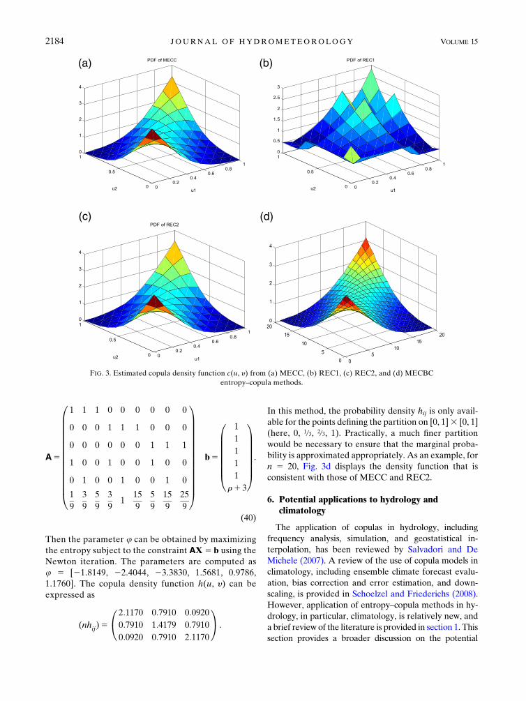
REC2 are shown in Figs. 3b and 3c, respectively. Given

the high bias of REC1, one can conclude that the REC1

density function may not be reliable. It is noted that the

REC2 density function is consistent with that of the

MECC given in Fig. 3a.

c. MECBC

The MECBC method is based on matching the

Spearman rank correlation coefficient 0.6 and the uni-

formly distributedmarginal property in the discrete form.

In the following bivariate (m 5 2) example, n 5 3 (see

section 4c) and thematrixH is defined on the space [0, 1]3[0, 1] as

H5

264h11 h12 h13h21 h22 h23h31 h32 h33

375 .

The n3m (here, 6) constraints can bewritten explicitly as

13 h111 13h121 13 h13 1 03 h21 1 03 h22 1 03 h23

1 03 h31 1 03 h32 1 03 h33 5 1,

(36)

03 h111 13h121 03 h13 1 03 h21 1 13 h22 1 03 h23

1 03 h31 1 13 h32 1 03 h33 5 1,

(37)

and

03 h111 03h121 13 h13 1 03 h21 1 03 h22 1 13 h23

1 03 h31 1 03 h32 1 13 h33 5 1.

(38)

The last constraint in the above equation is redundant

because it is automatically ensured by other constraints.

Thus, the total number of effective constraints isn3m2 1

(here, 5). Furthermore, the constraint for the Spearman

rank correlation coefficient can be expressed as

1

9[h111 3h121 5h13 1 3h21 1 9h22 1 15h23 1 5h31

1 15h32 1 25h33]5 r1 3. (39)

The above constraints can be written in the matrix form

AX 5 b as

FIG. 2. Biases of the marginal distributions for the (from top to bottom) MECC, REC1, and

REC2 entropy–copula methods.

DECEMBER 2014 AGHAKOUCHAK 2183

A5

0BBBBBBBBBBBBBB@

1 1 1 0 0 0 0 0 0

0 0 0 1 1 1 0 0 0

0 0 0 0 0 0 1 1 1

1 0 0 1 0 0 1 0 0

0 1 0 0 1 0 0 1 0

1

9

3

9

5

9

3

91

15

9

5

9

15

9

25

9

1CCCCCCCCCCCCCCA

b5

0BBBBBBB@

1

1

1

1

1

r1 3

1CCCCCCCA.

(40)

Then the parameter u can be obtained by maximizing

the entropy subject to the constraint AX5 b using the

Newton iteration. The parameters are computed as

u 5 [21.8149, 22.4044, 23.3830, 1.5681, 0.9786,

1.1760]. The copula density function h(u, y) can be

expressed as

(nhij)5

0@ 2:1170 0:7910 0:0920

0:7910 1:4179 0:7910

0:0920 0:7910 2:1170

1A .

In this method, the probability density hij is only avail-

able for the points defining the partition on [0, 1]3 [0, 1]

(here, 0, 1/3, 2/3, 1). Practically, a much finer partition

would be necessary to ensure that the marginal proba-

bility is approximated appropriately. As an example, for

n 5 20, Fig. 3d displays the density function that is

consistent with those of MECC and REC2.

6. Potential applications to hydrology andclimatology

The application of copulas in hydrology, including

frequency analysis, simulation, and geostatistical in-

terpolation, has been reviewed by Salvadori and De

Michele (2007). A review of the use of copula models in

climatology, including ensemble climate forecast evalu-

ation, bias correction and error estimation, and down-

scaling, is provided in Schoelzel and Friederichs (2008).

However, application of entropy–copula methods in hy-

drology, in particular, climatology, is relatively new, and

a brief review of the literature is provided in section 1. This

section provides a broader discussion on the potential

FIG. 3. Estimated copula density function c(u, y) from (a) MECC, (b) REC1, (c) REC2, and (d) MECBC

entropy–copula methods.

2184 JOURNAL OF HYDROMETEOROLOGY VOLUME 15

applications of entropy–copula methods in hydrology

and climatology, followed by an example application.

a. Climate change detection and analysis

Numerous studies have shown/argued that climate

extremes have been changing in the past and may

change in the future as well (Alexander et al. 2006; Hao

et al. 2013; Estrella and Menzel 2013; Damberg and

AghaKouchak 2014; Mehran et al. 2014; Madani and

Lund 2010; Hansen et al. 2010; Easterling et al. 2000;

AghaKouchak et al. 2012). Several empirical statistical

indices have been developed that can be used to quan-

tify changes in weather and climate extremes, including

annual temperature maxima and the number of dry days

(Schefzik 2011; Zhang et al. 2011) or categorical and vol-

umetricmeasures of climatic variables (AghaKouchak and

Mehran 2013). The minimum cross-entropy method could

potentially be used for detecting changes in climatic and

hydrologic extremes. As mentioned earlier, the minimum

cross-entropy method quantifies the distance between

(divergence of) one distribution and another. This model

can be used to quantify whether the distribution of tem-

perature or streamflow data has changed over time. Using

entropy–copula models reviewed in this study, one can

also investigate changes to the distributions (or extremes

of the distribution) of hydrologic–climatic variables in both

space (copula) and time (entropy). On the other hand,

climate variables are interdependent, and changes in one

variable may lead to changes in other variables as well. In

a recent study, Hao et al. (2013) assessed changes in con-

current precipitation and temperature extremes and re-

ported substantial changes in concurrent extremes. Given

the properties of entropy–copula models, they can be used

to assess climate change and variability based on multiple

variables and their joint distribution.

b. Uncertainty and error analysis

In the past three decades, the development of satel-

lite precipitation datasets and weather radar systems

has provided remotely sensed gridded data at the

global-scale variables to the community (Stedinger

et al. 1985; Sorooshian et al. 2011). However, remotely

sensed precipitation datasets are subject to retrieval

errors and uncertainties (Lee 2012; Mehran and

AghaKouchak 2014; Ebtehaj and Foufoula-Georgiou

2013; Tian et al. 2009). In addition to remote sensing

techniques, global climate models have been widely

used to simulate the climate of the past and future.

However, climate simulations are also highly uncertain,

and the biases and errors associated with climate data

have been discussed in numerous publications (Westra

et al. 2007; Serinaldi 2009; Mehran et al. 2014; Liu et al.

2014). Thus far, a number of uncertainty models have

been developed for satellite and radar data, as well as

climate model simulations (Stedinger and Vogel 1984;

Koutsoyiannis 1994; AghaKouchak et al. 2010b,c; Mölleret al. 2012), from which limited models account for both

space–time properties of errors and uncertainties. The

introduced entropy–copula method could potentially be

used for developing error models for remotely sensed

data and climate model simulations upon availability of

ground-based point observations of error (i.e., gridded

remotely sensed or climate model-based precipitation

data and reference gauge observations). The error at the

observation locations can be used to build the de-

pendence structure of the error using the introduced

entropy–copulamodels. One can then simulate stochastic

models of space–time error in order to derive an en-

semble of remotely sensed or model-based simulations as

a measure of uncertainty.

c. Bias correction and downscaling

In addition to developing error models, the entropy–

copula models can be utilized for bias correction and

downscaling of dependent variables. Bias correction or

downscaling of coarse climate data are often carried out

before using climate model outputs in climate change

impact studies (Chen et al. 2011; Hagemann et al. 2011).

Traditionally, the bias correction and also downscaling

are conducted for individual variables (e.g., pre-

cipitation and temperature) independently, ignoring the

relationship that may exist between climatic variables.

In a recent study, Piani and Haerter (2012) proposed

that the empirical copula be used for simultaneous bias

correction of temperature and precipitation data. This

approach was a major breakthrough in multivariate bias

correction.While themethodology outlined in Piani and

Haerter (2012) considers the relationship between pre-

cipitation and temperature for bias correction, it does

not necessarily preserve the rank correlation before and

after bias adjustment. Entropy–copula models can be

used for multivariate bias correction while preserving

the rank correlation, because the observed rank corre-

lation can be used as a constraint in the model. Similar

models can also be developed for downscaling and dis-

aggregation of multiple dependent climate variables.

d. High-dimensional problems

In many applications (e.g., spatial error analysis and

downscaling), the problem in hand involves multiple

variables or the many vectors of the same variable across

a large region (e.g., pixel-based precipitation data).While

there are a number of copula families that can be used

in high-dimensional studies [e.g., vine copula (Bedford

and Cooke 2002) and Plackett family copula (Kao and

Govindaraju 2008)], copula families that have been

DECEMBER 2014 AGHAKOUCHAK 2185

widely used in hydrology (i.e., Archimedean copulas) are

mainly suitable for bivariate or trivariate problems. In

general, extension of Archimedean copulas for high-

dimensional problems is not straightforward, and hence,

their use for studies that involve a large number of vari-

ables is restricted to certain conditions (Joe 1997; McNeil

and Ne�slehová 2009; McNeil 2008). Given the properties

of entropy–copula models (Hao and Singh 2013), dis-

cussed earlier, they offer a unique opportunity for sta-

tistical analysis of high-dimensional problems (see, e.g.,

Friedman and Huang 2010).

e. Frequency analysis

Entropy–copula models can be used for multivariate

frequency analysis. This requires modeling the de-

pendence structure of the variables involved (e.g., such

as flood volume and peak) and can be achieved by fitting

a multivariate parametric distribution (Favre et al. 2004;

Shiau et al. 2006; Genest et al. 2007; Sadri and Burn

2012). As an example application, the entropy–copula

concept is applied to flood frequency analysis to illus-

trate construction of the density function c(u, y) using

the entropy–copula. Here, only the MECC is employed

because its joint density function is continuous and

hence is more appropriate for flood frequency analysis.

The flood peak flow (Q) and volume (V) data extracted

from the daily streamflow data from 1963 to 1995 from the

Saguenay region in Quebec, Canada, are used for bi-

variate frequency analysis (Yue et al. 1999; Chebana and

Ouarda 2011; Zhang and Singh 2007). In this case study,

the maximum entropy copula is employed to model the

dependence structure of the flood peak and volume, and

the Gumbel distribution is used to model the marginal

distribution. For the maximum entropy copula, the first

three moments up to order 3 and the pairwise product of

the marginal probability are used. The joint return period

in which either the flood volume or flood peak or both

exceed the threshold level can be expressed as

TDS 51

P(D$d or S$ s)5

1

12C(u, y).

The flood peak and volume based on the maximum

entropy copula is shown in Fig. 4. The figure provides

multivariate return period information based on both

flood peak and volume.

The potential applications of the entropy–copula

models are not limited to the above examples. In

general, these methods could be applied to problems

that involve space–time dependence, such as geo-

statistical interpolation, downscaling, evaluation of

ensemble climate forecasts, regional extreme value

analysis, etc. In the future, more studies are expected

to use entropy–copula methods to address challenges

in hydrology and climate data analysis.

7. Conclusions and remarks

The entropy and copula concepts have been shown to

be powerful tools in various applications in hydrology,

climatology, and other areas. In recent years, new

methods have been proposed for developing copulas

based on the maximum entropy theory (entropy–copula).

These copulas provide the opportunity to derive prob-

ability distribution function of multiple dependent var-

iables and their dependence structure. This study

reviews the recent developments in entropy–copula and

broadly classifies them into three main groups based on

their model structures: 1) continuous maximum entropy

copula (CMEC), 2) mixed maximum entropy copula

(MMEC), and 3) discrete density maximum entropy

copula (DDMEC). The three categories of the entropy–

copula models differ in the type of constraints (i.e.,

uniformly distributed marginal and dependence struc-

ture) used to derive the copula density within the max-

imumentropy framework.After a detailed discussion on

different entropy–copula modeling concepts, a simple

numerical example is used for illustrating different

methods, followed by an example application to bi-

variate flood frequency analysis.

The CMEC method uses the continuous functions of

the marginal probabilities as the constraints to derive

the copula density function. The numerical example

provided here, shows that themarginal probabilities and

the dependence structure can be preserved reasonably

well. The MMECmethod uses the discrete points of the

FIG. 4. Bivariate return period of the flood peak and volume based

on entropy–copula.

2186 JOURNAL OF HYDROMETEOROLOGY VOLUME 15

marginal probabilities and continuous functions of the

marginal probabilities (e.g., pairwise product) as con-

straints to derive the copula density. The relative en-

tropy copula, which belongs to the MMEC category,

offers an attractive property in which the prior distri-

bution can be incorporated into the derivation of the

copula family. The results show that, by increasing the

number of discrete points, modeling of the marginal

probability and dependence structure will be improved.

In the provided numerical example, the bias significantly

reduced after increasing the number of discrete points.

This indicates that, in a practical application, one can

improve the model performance by increasing the

number of discrete points. The DDMEC method dis-

cretizes both the marginal and joint constraints to derive

the copula density function. The marginal probability is

only available for the points defining the partition on the

univariate interval, and thus, in practice, a fine partition

is required. It should be noted that while DDMEC’s

joint density is not continuous, the resulting joint dis-

tribution itself is continuous.

The entropy–copula methods introduced in this study

have different properties and characteristics. Selecting

an appropriate entropy–copula method is problem-

specific, and one cannot simply generalize the best

choice of entropy–copula method. For any specific ap-

plication, various entropy–copula models should be

tested and validated to identify a representative model

for the problem at hand. For example, when dealing

with a multidimensional problem (say, dimension .3),

the CMEC will be less computationally demanding than

the other methods because the marginal property is

approximated with the moments of the marginal prob-

abilities instead of the probabilities at discrete points.

While entropy–copula models provide opportunities

to advance multivariate statistical modeling, they have

their own limitations. For many types of entropy–copula

models there is no analytical solution for optimization and

parameter estimation. Therefore, numerical methods or

sampling approaches should be used to estimate the pa-

rameters. For high-dimensional problems, as the number

of parameters grows, parameter estimation becomesmore

computationally demanding. This review of the current

maximum entropy–copula methods sheds light on the

potential applications in hydrology and climatology.

However, these models are relatively new to hydrology

and climatology, and more research efforts in this di-

rection are required to fully explore their potential ap-

plications. Interested readers can request the source code

of the models discussed in this paper from the author.

Acknowledgments. The author thanks the three

anonymous reviewers for their thoughtful comments

and suggestions. The financial support for this study is

made available fromNational Science Foundation (NSF)

Award EAR-1316536. The author thanks Dr. Hao for his

inputs on an earlier draft of this paper.

REFERENCES

AghaKouchak, A., and A. Mehran, 2013: Extended contingency

table: Performance metrics for satellite observations and cli-

mate model simulations. Water Resour. Res., 49, 7144–7149,

doi:10.1002/wrcr.20498.

——, A. Bárdossy, and E. Habib, 2010a: Conditional simulation

of remotely sensed rainfall data using a non-Gaussian

v-transformed copula. Adv. Water Resour., 33, 624–634,

doi:10.1016/j.advwatres.2010.02.010.

——, ——, and ——, 2010b: Copula-based uncertainty modelling:

Application to multisensor precipitation estimates. Hydrol.

Processes, 24, 2111–2124, doi:10.1002/hyp.7632.——, E. Habib, and A. Bárdossy, 2010c: Modeling radar rainfall

estimation uncertainties: Random errormodel. J. Hydrol. Eng.,

15, 265–274, doi:10.1061/(ASCE)HE.1943-5584.0000185.

——, D. Easterling, K. Hsu, S. Schubert, and S. Sorooshian, Eds.,

2012: Extremes in a Changing Climate. Springer, 423 pp.

Alexander, L., and Coauthors, 2006: Global observed changes in

daily climate extremes of temperature. J. Geophys. Res., 111,

D05109, doi:10.1029/2005JD006290.

Ané, T., and C. Kharoubi, 2003: Dependence structure and risk

measure. J. Bus., 76, 411–438, doi:10.1086/375253.

Balakrishnan, N., and C. D. Lai, 2009: Continuous Bivariate Dis-

tributions. 2nd ed. Springer, 684 pp.

Bárdossy, A., 2006: Copula-based geostatistical models for

groundwater quality parameters. Water Resour. Res., 42,

W11416, doi:10.1029/2005WR004754.

Bedford, T., and R. M. Cooke, 2002: Vines—A new graphical

model for dependent random variables. Ann. Stat., 30, 1031–

1068, doi:10.1214/aos/1031689016.

Borwein, J. M., and A. S. Lewis, 2010: Convex Analysis and Non-

linear Optimization: Theory and Examples. 2nd ed. CMS

Books in Mathematics, Vol. 3, Springer, 310 pp.

Brunsell, N. A., 2010: A multiscale information theory approach to

assess spatial–temporal variability of daily precipitation. J. Hy-

drol., 385, 165–172, doi:10.1016/j.jhydrol.2010.02.016.

Chebana, F., and T. Ouarda, 2011: Multivariate quantiles in hydro-

logical frequency analysis.Environmetrics, 22, 63–78, doi:10.1002/env.1027.

Chen, C., J. O. Haerter, S. Hagemann, and C. Piani, 2011: On the

contribution of statistical bias correction to the uncertainty in

the projected hydrological cycle. Geophys. Res. Lett., 38,L20403, doi:10.1029/2011GL049318.

Chu, B., 2011: Recovering copulas from limited information and an

application to asset allocation. J. Bank. Finance, 35, 1824–1842, doi:10.1016/j.jbankfin.2010.12.011.

——, and S. Satchell, 2005: On the recovery of the most entropic

copulas from prior knowledge of dependence. CiteSeer. [Avail-

able online at http://citeseerx.ist.psu.edu/viewdoc/summary?doi510.1.1.125.2326.]

Chui, C., and X.Wu, 2009: Exponential series estimation of empirical

copulas with application to financial returns. Adv. Econom., 25,

263–290, doi:10.1108/S0731-9053(2009)0000025011.

Damberg, L., and A. AghaKouchak, 2014: Global trends and

patterns of droughts from space. Theor. Appl. Climatol., 117,

441–448, doi:10.1007/s00704-013-1019-5.

DECEMBER 2014 AGHAKOUCHAK 2187

Dempster, M. A. H., E. A. Medova, and S. W. Yang, 2007: Em-

pirical copulas for CDO tranche pricing using relative en-

tropy. Int. J. Theor. Appl. Finance, 10, 679–701, doi:10.1142/

S0219024907004391.

Durrett, R., 2005: Probability: Theory and Examples. Brooks/Cole

Publishing, 528 pp.

Easterling, D., G. Meehl, C. Parmesan, S. Changnon, T. Karl,

and L. Mearns, 2000: Climate extremes: Observations,

modeling, and impacts. Science, 289, 2068–2074, doi:10.1126/

science.289.5487.2068.

Ebtehaj, A. M., and E. Foufoula-Georgiou, 2013: On variational

downscaling, fusion, and assimilation of hydrometeorological

states: A unified framework via regularization. Water Resour.

Res., 49, 5944–5963, doi:10.1002/wrcr.20424.

Estrella, N., and A. Menzel, 2013: Recent and future climate ex-

tremes arising from changes to the bivariate distribution of

temperature and precipitation in Bavaria, Germany. Int.

J. Climatol., 33, 1687–1695, doi:10.1002/joc.3542.

Favre,A.-C., S. ElAdlouni, L. Perreault,N.Thiémonge, andB.Bobée,2004: Multivariate hydrological frequency analysis using copulas.

Water Resour. Res., 40, W01101, doi:10.1029/2003WR002456.

Friedman, C. A., and J. Huang, 2010: Most entropic copulas:

General form, and calibration to high-dimensional data in an

important special case. Social Science Research Network,

doi:10.2139/ssrn.1725517.

Genest, C., and A. C. Favre, 2007: Everything you always wanted to

know about copula modeling but were afraid to ask. J. Hydrol.

Eng., 12, 347–368, doi:10.1061/(ASCE)1084-0699(2007)12:4(347).

——, A.-C. Favre, J. Béliveau, and C. Jacques, 2007: Metaelliptical

copulas and their use in frequency analysis of multivariate hy-

drological data. Water Resour. Res., 43, W09401, doi:10.1029/

2006WR005275.

Grimaldi, S., and F. Serinaldi, 2006: Asymmetric copula in multi-

variate flood frequency analysis.Adv.Water Resour., 29, 1155–

1167, doi:10.1016/j.advwatres.2005.09.005.

Hagemann, S., C. Chen, J. O. Haerter, J. Heinke, D. Gerten, and

C. Piani, 2011: Impact of a statistical bias correction on the

projected hydrological changes obtained from three GCMs and

two hydrologymodels. J. Hydrometeor., 12, 556–578, doi:10.1175/

2011JHM1336.1.

Hansen, J., R. Ruedy, M. Sato, and K. Lo, 2010: Global surface

temperature change. Rev. Geophys., 48,RG4004, doi:10.1029/

2010RG000345.

Hao, Z., and V. Singh, 2011: Single-site monthly streamflow sim-

ulation using entropy theory.Water Resour. Res., 47,W09528,

doi:10.1029/2010WR010208.

——, and ——, 2012: Entropy-copula method for single-site

monthly streamflow simulation. Water Resour. Res., 48,

W06604, doi:10.1029/2011WR011419.

——, and A. AghaKouchak, 2013: Multivariate standardized

drought index: A parametric multi-index model. Adv. Water

Resour., 57, 12–18, doi:10.1016/j.advwatres.2013.03.009.——, and V. Singh, 2013: Modeling multi-site streamflow de-

pendence with maximum entropy copula.Water Resour. Res.,

49, 7139–7143, doi:10.1002/wrcr.20523.

——, and A. AghaKouchak, 2014: A nonparametric multivariate

multi-index drought monitoring framework. J. Hydrometeor.,

15, 89–101, doi:10.1175/JHM-D-12-0160.1.

——,——, and T. J. Phillips, 2013: Changes in concurrent monthly

precipitation and temperature extremes.Environ. Res. Lett., 8,

034014, doi:10.1088/1748-9326/8/3/034014.

Jaynes, E. T., 1957a: Information theory and statistical mechanics.

Phys. Rev., 106, 620–630, doi:10.1103/PhysRev.106.620.

——, 1957b: Information theory and statistical mechanics. II. Phys.

Rev., 108, 171–190, doi:10.1103/PhysRev.108.171.

Joe, H., 1997: Multivariate Models and Dependence Concepts.

Chapman & Hall, 424 pp.

Kao, S. C., and R. S. Govindaraju, 2008: Trivariate statistical

analysis of extreme rainfall events via the Plackett family of

copulas. Water Resour. Res., 44, W02415, doi:10.1029/

2007WR006261.

Kapur, J., 1989: Maximum-Entropy Models in Science and Engi-

neering. John Wiley & Sons, 635 pp.

Kesavan, H., and J. Kapur, 1992: Entropy Optimization Principles

with Applications. Academic Press, 408 pp.

Kolesárová, A., R. Mesiar, J. Mordelová, and C. Sempi, 2006:

Discrete copulas. IEEE Trans. Fuzzy Syst., 14, 698–705,

doi:10.1109/TFUZZ.2006.880003.

Kotz, S., N. Balakrishnan, and N. L. Johnson, 2000: Continuous

Multivariate Distributions: Models and Applications. Vol. 1.

Wiley-Interscience, 752 pp.

Koutsoyiannis, D., 1994: A stochastic disaggregation method for

design storm and flood synthesis. J. Hydrol., 156, 193–225,

doi:10.1016/0022-1694(94)90078-7.

Kullback, S., and R. Leibler, 1951: On information and sufficiency.

Ann. Math. Stat., 22, 79–86, doi:10.1214/aoms/1177729694.

Lee, T., 2012: Serial dependence properties in multivariate

streamflow simulation with independent decomposition anal-

ysis. Hydrol. Processes, 26, 961–972, doi:10.1002/hyp.8177.

Liu, Z., A. Mehran, T. J. Phillips, and A. AghaKouchak, 2014:

Seasonal and regional biases in CMIP5 precipitation simula-

tions. Climate Res., 60, 35–50, doi:10.3354/cr01221.Madani, K., and J. R. Lund, 2010: Estimated impacts of climate

warming on California’s high-elevation hydropower. Climatic

Change, 102, 521–538, doi:10.1007/s10584-009-9750-8.

Mayor, G., J. Suñer, and J. Torrens, 2005: Copula-like operations

on finite settings. IEEE Trans. Fuzzy Syst., 13, 468–477,

doi:10.1109/TFUZZ.2004.840129.

McNeil, A. J., 2008: Sampling nested Archimedean copulas. J. Stat.

Comput. Simul., 78, 567–581, doi:10.1080/00949650701255834.

——, and J. Ne�slehová, 2009: Multivariate Archimedean copulas,

d-monotone functions and ‘1-norm symmetric distributions.

Ann. Stat., 37, 3059–3097.

Mead, L., and N. Papanicolaou, 1984: Maximum entropy in the

problem of moments. J. Math. Phys., 25, 2404–2417,

doi:10.1063/1.526446.

Meeuwissen, A. M. H., and T. Bedford, 1997: Minimally in-

formative distributions with given rank correlation for use in

uncertainty analysis. J. Stat. Comput. Simul., 57, 143–174,

doi:10.1080/00949659708811806.

Mehran, A., and A. AghaKouchak, 2014: Capabilities of satellite

precipitation datasets to estimate heavy precipitation rates at

different temporal accumulations. Hydrol. Processes, 28,

2262–2270, doi:10.1002/hyp.9779.

——, ——, and T. J. Phillips, 2014: Evaluation of CMIP5 conti-

nental precipitation simulations relative to satellite-based

gauge-adjusted observations. J. Geophys. Res. Atmos., 119,

1695–1707, doi:10.1002/2013JD021152.

Möller, A., and Coauthors, 2012: Multivariate probabilistic

forecasting using ensemble Bayesian model averaging and

copulas.Quart. J. Roy.Meteor. Soc., 139, 982–991, doi:10.1002/

qj.2009.

Nazemi, A., and A. Elshorbagy, 2012: Application of copula

modelling to the performance assessment of reconstructed

watersheds. Stochastic Environ. Res. Risk Assess., 26, 189–205,

doi:10.1007/s00477-011-0467-7.

2188 JOURNAL OF HYDROMETEOROLOGY VOLUME 15

Nelsen, R. B., 2006: An Introduction to Copulas. 2nd ed. Springer,

272 pp.

Phillips, S. J., R. P. Anderson, and R. E. Schapire, 2006: Maximum

entropy modeling of species geographic distributions. Ecol.

Modell., 190, 231–259, doi:10.1016/j.ecolmodel.2005.03.026.

Piani, C., and J. O. Haerter, 2012: Two dimensional bias correction

of temperature and precipitation copulas in climate models.

Geophys. Res. Lett., 39, L20401, doi:10.1029/2012GL053839.

Piantadosi, J., P. Howlett, and J. Boland, 2007:Matching the grade

correlation coefficient using a copula with maximum dis-

order. J. Ind. Manage. Optim., 3, 305–312, doi:10.3934/

jimo.2007.3.305.

——,——, and J. Borwein, 2012a: Copulas withmaximum entropy.

Optim. Lett., 6, 99–125, doi:10.1007/s11590-010-0254-2.

——, ——, ——, and J. Henstridge, 2012b: Maximum entropy

methods for generating simulated rainfall. Numer. Algebra

Control Optim., 2, 233–256, doi:10.3934/naco.2012.2.233.

Pougaza, D.-B., and A. Mohammad-Djafari, 2011: Maximum en-

tropies copulas. AIP Conf. Proc., 1305, 329, doi:10.1063/

1.3573634.

——, and ——, 2012: New copulas obtained by maximizing Tsallis

or Rényi entropies. AIP Conf. Proc., 1443, 238, doi:10.1063/

1.3703641.

——, ——, and J.-F. Bercher, 2010: Link between copula and to-

mography. Pattern Recognit. Lett., 31, 2258–2264, doi:10.1016/

j.patrec.2010.05.001.

Qu, L., and W. Yin, 2012: Copula density estimation by total var-

iation penalized likelihood with linear equality constraints.

Comput. Stat. Data Anal., 56, 384–398, doi:10.1016/

j.csda.2011.07.016.

——, H. Chen, and Y. Tu, 2011: Nonparametric copula density

estimation in sensor networks. Proc. MSN 2011: Seventh Int.

Conf. onMobileAd-Hoc and SensorNetworks,Beijing, China,

IEEE, doi:10.1109/MSN.2011.50.

Sadri, S., and D. H. Burn, 2012: Copula-based pooled frequency

analysis of droughts in the Canadian Prairies. J. Hydrol. Eng.,

19, 277–289, doi:10.1061/(ASCE)HE.1943-5584.0000603.

Salvadori, G., and C. De Michele, 2007: On the use of copulas in

hydrology: Theory and practice. J. Hydrol. Eng., 12, 369–380,

doi:10.1061/(ASCE)1084-0699(2007)12:4(369).

——, ——, N. T. Kottegoda, and R. Rosso, 2007: Extremes in

Nature: An Approach Using Copulas. Springer, 292 pp.

Schefzik, R., 2011: Ensemble copula coupling. Diploma thesis,

Faculty of Mathematics and Informatics, Heidelberg Univer-

sity, 149 pp.

Schoelzel, C., and P. Friederichs, 2008: Multivariate non-normally

distributed random variables in climate research–introduction

to the copula approach. Nonlinear Processes Geophys., 15,

761–772, doi:10.5194/npg-15-761-2008.

Serinaldi, F., 2009: A multisite daily rainfall generator driven by

bivariate copula-based mixed distributions. J. Geophys. Res.,

114, D10103, doi:10.1029/2008JD011258.

——, and S. Grimaldi, 2007: Fully nested 3-copula: Procedure and

application on hydrological data. J. Hydrol. Eng., 12, 420–430,

doi:10.1061/(ASCE)1084-0699(2007)12:4(420).

Shannon, C. E., 1948: Amathematical theory of communications.Bell

Syst. Tech. J., 27, 379–423, doi:10.1002/j.1538-7305.1948.tb01338.x.

Shiau, J.-T., H.-Y. Wang, and C.-T. Tsai, 2006: Bivariate frequency

analysis of floods using copulas. J. Amer. Water Resour. As-

soc., 42, 1549–1564, doi:10.1111/j.1752-1688.2006.tb06020.x.

Singh, V. P., 1992: Elementary Hydrology. Prentice Hall, 973 pp.

——, 1997: The use of entropy in hydrology and water

resources. Hydrol. Processes, 11, 587–626, doi:10.1002/

(SICI)1099-1085(199705)11:6,587::AID-HYP479.3.0.CO;2-P.

——, 2011: Hydrologic synthesis using entropy theory:

Review. J. Hydrol. Eng., 16, 421–433, doi:10.1061/

(ASCE)HE.1943-5584.0000332.

Sklar, A., 1959: Fonctions de répartition à n dimensions et leursmarges. Publ. Inst. Stat. Univ. Paris, 8, 229–231.

Sorooshian, S., and Coauthors, 2011: Advanced concepts on re-

mote sensing of precipitation at multiple scales. Bull. Amer.

Meteor. Soc., 92, 1353–1357, doi:10.1175/2011BAMS3158.1.

Stedinger, J. R., and R. M. Vogel, 1984: Disaggregation procedures

for generating serially correlated flow vectors. Water Resour.

Res., 20, 47–56, doi:10.1029/WR020i001p00047.

——, D. P. Lettenmaier, and R. M. Vogel, 1985: Multisite ARMA

(1, 1) and disaggregation models for annual streamflow

generation. Water Resour. Res., 21, 497–510, doi:10.1029/

WR021i004p00497.

——, R. M. Vogel, and E. Foufoula-Georgiou, 1993: Frequency

analysis of extreme events. Handbook of Hydrology, D. R.

Maidment, Ed., McGraw-Hill, 18.1–18.66.

Tian, Y., and Coauthors, 2009: Component analysis of errors in

satellite-based precipitation estimates. J. Geophys. Res., 114,

D24101, doi:10.1029/2009JD011949.

Trivedi, P. K., and D. M. Zimmer, 2005: Copula modeling: An

introduction for practitioners. Found. Trends Econometrics, 1,1–111, doi:10.1561/0800000005.

Vapnyarskii, I. B., 2001: Lagrange multipliers. Encyclopedia of

Mathematics, M. Hazewinkel, Ed., Springer, 1–8.

Venter, G. G., 2002: Tails of copulas.Proc. Casualty Actuarial Soc.,

89, 68–113. [Available online at http://casualtyactuaries.com/

library/studynotes/Venter_Tails_of_Copulas.pdf.]

Westra, S., C. Brown, U. Lall, and A. Sharma, 2007: Modeling

multivariable hydrological series: Principal component anal-

ysis or independent component analysis? Water Resour. Res.,

43, W06429, doi:10.1029/2006WR005617.

Yue, S., and Coauthors, 1999: The Gumbel mixed model for flood

frequency analysis. J. Hydrol., 226, 88–100, doi:10.1016/

S0022-1694(99)00168-7.

Zhang, L., and V. P. Singh, 2007: Bivariate rainfall frequency dis-

tributions usingArchimedean copulas. J. Hydrol., 332, 93–109,doi:10.1016/j.jhydrol.2006.06.033.

Zhang, X., L. Alexander, G. C. Hegerl, P. Jones, A. K. Tank, T. C.

Peterson, B. Trewin, and F. W. Zwiers, 2011: Indices for

monitoring changes in extremes based on daily temperature

and precipitation data. Wiley Interdiscip. Rev.: Climate

Change, 2, 851–870, doi:10.1002/wcc.147.

Zhao, N., and W. T. Lin, 2011: A copula entropy approach to

correlation measurement at the country level. Appl. Math.

Comput., 218, 628–642, doi:10.1016/j.amc.2011.05.115.

Zhu, S. C., Y. N. Wu, and D. Mumford, 1997: Minimax entropy

principle and its application to texture modeling. Neural

Comput., 9, 1627–1660, doi:10.1162/neco.1997.9.8.1627.

DECEMBER 2014 AGHAKOUCHAK 2189