See discussions, stats, and author profiles for this publication at: https://www.researchgate.net/publication/316828478

Entropy of radiation: The unseen side of light

Article  in  Scientific Reports · May 2017

DOI: 10.1038/s41598-017-01622-6

CITATIONS

0READS

46

1 author:

Some of the authors of this publication are also working on these related projects:

Entropy of Radiation View project

Alfonso Delgado-Bonal

NASA

10 PUBLICATIONS   7 CITATIONS   

SEE PROFILE

All content following this page was uploaded by Alfonso Delgado-Bonal on 10 May 2017.

The user has requested enhancement of the downloaded file.

1Scientific RepoRts | 7: 1642 | DOI:10.1038/s41598-017-01622-6

www.nature.com/scientificreports

Entropy of radiation: the unseen side of lightAlfonso Delgado-Bonal

Despite the fact that 2015 was the international year of light, no mention was made of the fact that radiation contains entropy as well as energy, with different spectral distributions. Whereas the energy function has been vastly studied, the radiation entropy distribution has not been analysed at the same speed. The Mode of the energy distribution is well known –Wien’s law– and Planck’s law has been analytically integrated recently, but no similar advances have been made for the entropy. This paper focuses on the characterization of the entropy of radiation distribution from an statistical perspective, obtaining a Wien’s like law for the Mode and integrating the entropy for the Median and the Mean in polylogarithms, and calculating the Variance, Skewness and Kurtosis of the function. Once these features are known, the increasing importance of radiation entropy analysis is evidenced in three different interdisciplinary applications: defining and determining the second law Photosynthetically Active Radiation (PAR) region efficiency, measuring the entropy production in the Earth’s atmosphere, and showing how human vision evolution was driven by the entropy content in radiation.

Entropy is a quantity as fundamental as energy, nevertheless, the analysis of the entropy content in radiation is not fully exploited yet. Although it has been applied in engineering and science, its existence is generally unknown and there are still many faces to explore.

The analysis of radiation entropy has been mainly carried out in the context of optics, whereas in other fields such as atmospheric physics or statistics the function has been studied only occasionally. The research in radiation entropy was very present at the beginnings of the quantum theory until the seminar paper of Bose1, who showed how to obtain Planck’s law without the necessity of determining the entropy of radiation. Soon after Planck pro-posed his radiation law and the associated equation for the spectral entropy, von Laue2 analysed the phenomena of interference from a thermodynamical perspective, discussing the applicability of the second law to radiation and the additivity of the entropy. His ideas were mostly continued in the fields of coherence and polariazation, where the radiation entropy approach has proven to be very productive3. In that sense, the importance of the radi-ation entropy in the scattering process is a field in current development, and the ideas are masterly investigated in ref. 4.

Although the optical properties have been investigated, the statistical ones have not received much attention, as well as the possible applications of the magnitude. It is the intention of this manuscript to amend this situation, and here I survey the statistical properties of the entropy of radiation and underline some new applications, which have not been investigated before in the knowledge of the author.

Planck’s laws for energy and entropy are density functions which are characterized by their Mode, Median and Mean. The Mode of Planck’s function is determined by the Wien’s displacement law, and it is well known that the maxima occur at different positions depending on the choice of the spectral variable5. The situation for the entropy of radiation is quite the same, and it is possible to determine its maxima as a Wien’s like law, with a different values of the coefficients depending on the selected spectral variable. This coefficient is a constant which cannot be obtained from the energy distribution.

The integration of Planck’s law in the whole spectrum gives directly the Stefan-Botlzmann’s law with the widely known dependence on the fourth power of the temperature, and the integration of the entropy gives the equivalent law with the third power dependence on the temperature. Although the complete integration is well known, the somehow incommodious mathematical form of the entropy distribution makes it not very suitable for integration in a region. In this paper, I show how to obtain a polylogarithmic expression to determine the entropy fractional emissive power of blackbody radiation in a given spectral band, and by making use of this expression, the Median and the Mode of the distribution are determined. Besides these measures of central tendency, the

University of Salamanca, Institute of Fundamental Physics and Mathematics, Pza. de la Merced S/N, 37008, Salamanca, Spain. Correspondence and requests for materials should be addressed to A.D. (email: alfonso_delgado@usal.es)

Received: 18 August 2016

Accepted: 3 April 2017

Published: xx xx xxxx

OPEN

www.nature.com/scientificreports/

2Scientific RepoRts | 7: 1642 | DOI:10.1038/s41598-017-01622-6

most important measures of variability are studied in this manuscript, which are the Variance, Skewness and Kurtosis, and a general expression for the moment of order n is provided.

The field of entropy radiative transfer is not fully developed yet, but it is of the utmost importance in many different fields such as heat transfer by radiation, climate sciences or information theory, and the interest in this magnitude has increased recently. One of the issues that held back the analysis of the entropy of radiation was the lack of direct applications, and in this paper I show how the concept can be applied to three different fields.

By making use of the two laws of thermodynamics and the expressions of the energy and entropy of radiation, the maximum obtainable work from radiation can be determined, a magnitude which is called exergy6, 7. This kind of analysis –named second law analysis– allows us to determine not only the amount of energy but also its quality, greatly important in industrial processes and, in particular, in solar energy conversion devices. Although the concept is currently being used, the determination of the exergy in spectral regions has been carried out by numerical procedures up to now. The analytical expression to determine the fractional emissive power for the exergy is derived here, which permits the analysis of the obtainable work from radiation in a determined band or spectral region more quickly and accurately. When the whole spectrum is considered, the expression is reduced to the well known Petela’s equation8.

One of the most important processes which makes use of radiation is photosynthesis. However, at the same time than the organism is obtaining energy from radiation, the organism is losing energy itself by emitting radia-tion, as a consequence of its own temperature. Thus, the exergy concept is more suitable to analyze the efficiency of the process, and the second law efficiency of the photosynthetic active radiation (PAR) region is defined and determined here using this formalism.

The spectral entropy law –which is the entropy of bosons– plays a role in the radiative transfer of entropy equivalent to the Planck’s law in classical radiative transfer. Even though the expression for the entropy of radi-ation used in this manuscript was proposed for the equilibrium situation, it has been proved that the equation holds for non-equilibrium situations9–11. By definition, blackbody radiation is that radiation which produces the largest amount of entropy for a given quantity of energy12. By characterizing the entropy content in blackbody radiation, it is possible to define more accurately the deviations from this kind of radiation.

In particular, the entropy expression can be applied to the analysis of radiation in the atmosphere. Here I present the entropy spectrum for Earth’s upwelling radiation, with the intention to show more applications of the entropy analysis. By comparison between the obtained values and those expected for a blackbody, the entropy production is characterized in a wavelength basis, showing that different absorption bands lead to different values of entropy production in the atmosphere. Therefore, the contribution of the different chemical species to the atmospheric entropy production budget can be inferred from this sort of analysis.

The entropy concept is applied in many disciplines besides engineering and science. In particular, information theory13 makes a very interesting use of the entropy magnitude, understanding it in relation with the information contained in a system. In a previous number of this journal14, I hypothesized that entropy plays a major role as driving force in the biological evolution of human eyesight, by determining the maximum of this function. Using the equations determined in this paper, I prove that the importance of the entropy in human vision is independ-ent of the spectral variable15, opening new ways to understand human perception and inference.

Finally, some mathematical appendixes complete this paper with the required explanations and demonstra-tions, including a short introduction to the historical development of the field for the interested reader.

The Mode: Wien’s law for the entropy of radiationThe expressions for energy (L) and entropy (S) of blackbody radiation in wavelength and frequency are:

λ=

−λ

λ

L hc

e

2 1

1 (1)hck T

2

5

λλ λ λ λ

=

+

+

−

λλ λ λ λS kc L

hcL

hcL

hcL

hc2 1

2log 1

2 2log

2 (2)4

5

2

5

2

5

2

5

2

and

ν=

−ν ν

L hc e

2 1

1 (3)hkT

3

2

ν=

+

−

+

−

−

−

−

ν ν ν ν νS k

c e e e e1 1

1log 1 1

1

1

1log 1

1 (4)hkT

hkT

hkT

hkT

2

2

Expressions 1–4 were firstly obtained by Planck16, and were demonstrated later by many other ways1, 17, including non-equilibrium situations9.

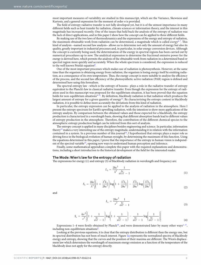
Looking at the previous equations, it is clear that the entropy distribution is different than the energy one, but its spectral distribution has not been of much interest. Figure 1a represents the normalized spectra of blackbody energy and entropy, showing that the curves and the position of their maxima are different. The Wien’s displace-ment law which determines the wavelength of maximum energy emission as a function of the temperature of the blackbody does not apply for the entropy directly.

www.nature.com/scientificreports/

3Scientific RepoRts | 7: 1642 | DOI:10.1038/s41598-017-01622-6

Using Equations 2 and 4, the statistical properties of the entropy of radiation can be analysed. The function is non-symmetric, it is always positive (because it is a density function), it has only one maximum, and the total integration gives the equivalent Stefan-Boltzmann’s law, S = 4/3σT3. The wavelength corresponding to the max-imum of the distribution depends on the temperature, as shown in Fig. 1b for different blackbody temperatures.

This behaviour resembles the energy distribution, and will be determined below by a Wien’s like law with a different coefficient. As in the case of the energy, the value of the constant (which determines the “position” of the maxima) will depend on the spectral variable used in the description of radiation, and it will be determined based on a parameter called dispersion rule coefficient, m18.

Energy and entropy distribution laws are density functions and the exchange between spectral variables must be carried out using differential terms. In particular, the relation between wavelength and frequency is

λ ν λ= −λνλ νS T S T( , ) ( ( ), )d

d, where ν λ λ= −d d c/ / 2. Generalizing this situation, it is possible to express the

entropy function Sϑ as a density distribution function defined differentially by:

= ϑϑ ϑdW S d (5)

where Wϑ represents the entropy emissive power in the differential interval dϑ. In this way it is clear that the emissive power is independent on the selected spectral variable, and the function Sϑ represents the spectral entropy emissive power per unit physical quantity interval ϑ from a blackbody at absolute temperature T. The different choices of spectral variables, such as wavelength, frequency, squared wavelength, etc., are studied here in terms of the dispersion rules19.

The Mode of the distribution is obtained from the condition dS/dϑ = 0. When the analysis is performed in frequency, dS/dν = 0, the transcendental equation which determines the maximum of the distribution is (see Appendix A):

− + − − + −

− − − =x e x e x e

ee xe e3 ( 1) 3 ( 1) ( ) 2 log 1

1( 1) ( 1) 0

(6)x x x

xx x x2 2 2 2

which can be numerically solved, obtaining the value of x = 2.538231893. Undoing the change of variable = νx hkT

, the peak is accomplished at:

ν= . × − −

TK s5 28882 10 (7)

max 10 1 1

In the case of the energy distribution, the maximum occurs at 5.87893 × 1010 K−1 s−1, a value slightly different.Similarly, in the case of wavelength starting from Equation 2 and doing the change of variable =

λx hc

kT, the

transcendental equation is ref. 14:

− + − − + −

− − − =x e x e x e

ee xe e5 ( 1) 5 ( 1) ( ) 4 log 1

1( 1) ( 1) 0

(8)x x x

xx x x2 2 2 2

The solution of the equation is x = 4.7912673578 and, undoing the change of variable, the Wien’s entropy displacement law in wavelength looks like:

λ = = . × −T b 3 00292 10 mK (9)entropy3

different than the value of benergy = 2.89777 × 10−3 m K.Looking at Equations 6 and 8, it is easy to generalize the transcendental equation to any value of the dispersion

coefficient, m. The general transcendental equation reads:

⋅ − + ⋅ − − + − ⋅ −

− − − =m x e m x e x e m

ee xe e( 1) ( 1) ( ) ( 1) log 1

1( 1) ( 1) 0

(10)x x x

xx x x2 2 2 2

Figure 1. (a) (left): Normalized entropy (blue line) and energy (red line) of blackbody radiation at 5800 K. The ratio entropy-to-energy is determined by the black line. (b) (right): Entropy of blackbody radiation at different temperatures. The behaviour resembles the energy distribution.

www.nature.com/scientificreports/

4Scientific RepoRts | 7: 1642 | DOI:10.1038/s41598-017-01622-6

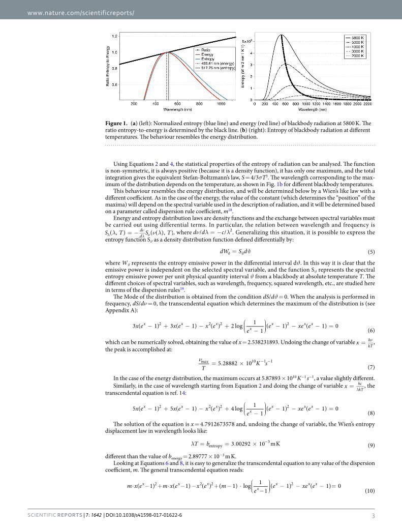
Which can be solved for each value of m. The values of the Wien’s coefficients are given in Table 1, along with the explanation of the dispersion rule used.

The Median: fractional emissive power of entropyIn the previous section, I characterized the wavelength of maximum emission of entropy by a blackbody emitter. Although the maximum of the spectral distribution of entropy is of critical importance, the knowledge of the entropy emissive power in a spectral region is required in the fields of radiative transfer, engineering and climate sciences, for example.

The determination of the fractional emissive power is usually done numerically, despite the fact that analytical expressions are tremendously advantageous in computing and provide an intrinsic elegance to the solution of the problem. In the field of thermal radiation, Planck’s equation is conventionally integrated using numerical pro-cedures, albeit an analytical solution in the form of polylogarithms has appeared recently in the literature20. The definition and properties of polylogarithms are briefly reviewed in Appendix C.

Although less known, the entropy of radiation has a different radiative transfer equation21, 22 and the source function is a nonlinear complex function. By making use of polylogarithms, an analytical expression for the integration of the entropy of radiation is achieved here. Moreover, after straightforward arithmetical transfor-mations, the solution is as simple as the expression for the energy and the calculations can be recycled, saving loads of computer time and attaining the best accuracy possible. With this expression it is possible to compute the entropy fractional emissive power, in particular the Median of the spectral entropy distribution, as well as any other percentile.

The fractional emissive power of isotropic blackbody radiation has been recently determined analytically as ref. 20:

πσ= + + +− − − −I T x Li e x Li e xLi e Li e15 { ( ) 3 ( ) 6 ( ) 6 ( )}

(11)Lx x x x

44 3

12

2 3 4

The polylogarithmic term of Equation 11 when the whole spectrum is studied is π15

4, and therefore the total flux is

given by the well known Stefan-Boltzmann’s law σT4. Dividing Equation 11 by the total energy flux σT4, the nor-malized fractional emissive power is then determined as:

π= + + +− − − −I x Li e x Li e xLi e Li e15 { ( ) 3 ( ) 6 ( ) 6 ( )}

(12)L normx x x x

, 43

12

2 3 4

The entropy fractional emissive power of isotropic radiation has not been analysed up to the date. Using a similar procedure, it is determined here as (see Appendix D):

πσ= + + +− − − −I T x Li e x Li e xLi e Li e15 { ( ) 4 ( ) 8 ( ) 8 ( )}

(13)Sx x x x

43 3

12

2 3 4

The total flux is obtained when the whole spectrum is considered. In such situation, the polylogarithmic term is reduced to π4

45

4 and the total entropy flux is given by the equivalent Stefan-Boltzmann’s law σT4

33. The emissive

power normalized to the total entropy flux is therefore given by:

π= + + +− − − −I x Li e x Li e xLi e Li e45

4{ ( ) 4 ( ) 8 ( ) 8 ( )}

(14)S normx x x x

, 43

12

2 3 4

It is noticeable that software such as Mathematica gives a more complex solution, which can be proved to be the same when only the real part is considered, differing only in an arbitrary integration constant23. The solution provided here is the simplest solution available, and has the advantage that the terms required for its calculation

ϑ Bϑ (T)dϑ Dispersion rule m Energy Entropy

ν2 ν ννB T d2 ( )2 frequency-squared 2. …

hckB(1 593624 ) . …

hckB(1 178179641 )

ν Bν(T)dν linear frequency 3. …

hckB(2 821439 ) . …

hckB(2 538231893 )

ν νν νB T d( )1

2square root frequency 7/2

. …hc

kB(3 380946 ) . …hc

kB(3 137016422 )

log ν νν νB T d( )1

log logarithmic frequency 4. …

hckB(3 920690 ) . …

hckB(3 706085183 )

log λ λλ λB T d( )1

log logarithmic wavelength 4. …

hckB(3 920690 ) . …

hckB(3 706085183 )

λ λλ λB T d( )1

2square root wavelength 9/2

. …hc

kB(4 447304 ) . …hc

kB(4 255382544 )

λ Bλ(T)dλ linear wavelength 5. …

hckB(4 965114 ) . …

hckB(4 791267357 )

λ2 λ λλB T d2 ( )2 wavelength-squared 6. …

hckB(5 984901 ) . …

hckB(5 838126229 )

Table 1. Wien’s peaks for the energy and the entropy of radiation for different dispersion rules, corresponding to different values of the dispersion coefficient m.

www.nature.com/scientificreports/

5Scientific RepoRts | 7: 1642 | DOI:10.1038/s41598-017-01622-6

are the same than those required for the energy fractional emissive power, which is translated in much less com-putational power.

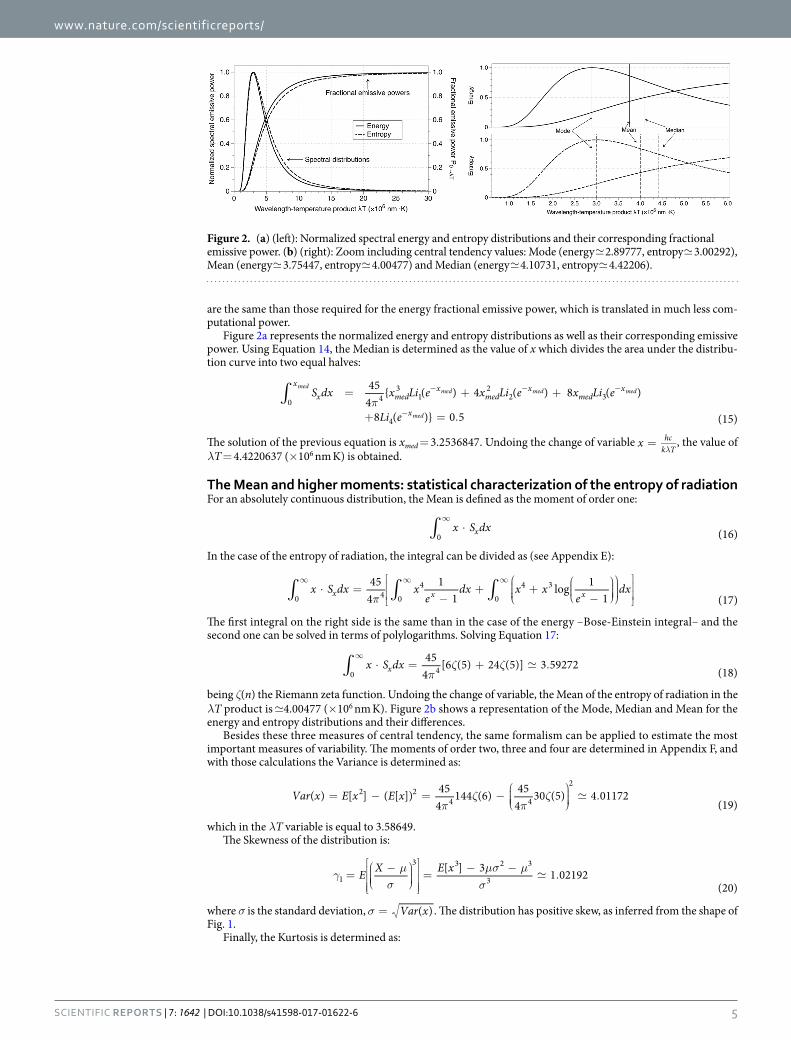
Figure 2a represents the normalized energy and entropy distributions as well as their corresponding emissive power. Using Equation 14, the Median is determined as the value of x which divides the area under the distribu-tion curve into two equal halves:

∫ π= + +

+ = .

− − −

−

S dx x Li e x Li e x Li e

Li e

454

{ ( ) 4 ( ) 8 ( )

8 ( )} 0 5 (15)

xx med

xmed

xmed

x

x0 4

31

22 3

4

medmed med med

med

The solution of the previous equation is xmed = 3.2536847. Undoing the change of variable =λ

x hck T

, the value of λT = 4.4220637 (×106 nm K) is obtained.

The Mean and higher moments: statistical characterization of the entropy of radiationFor an absolutely continuous distribution, the Mean is defined as the moment of order one:

∫ ⋅∞

x S dx (16)x0

In the case of the entropy of radiation, the integral can be divided as (see Appendix E):

∫ ∫ ∫π⋅ =

−

+

+ −

∞ ∞ ∞x S dx x

edx x x

edx45

41

1log 1

1 (17)x x x0 4 0

4

0

4 3

The first integral on the right side is the same than in the case of the energy –Bose-Einstein integral– and the second one can be solved in terms of polylogarithms. Solving Equation 17:

∫ πζ ζ⋅ = + .

∞x S dx 45

4[6 (5) 24 (5)] 3 59272

(18)x0 4

being ζ(n) the Riemann zeta function. Undoing the change of variable, the Mean of the entropy of radiation in the λT product is 4.00477 (×106 nm K). Figure 2b shows a representation of the Mode, Median and Mean for the energy and entropy distributions and their differences.

Besides these three measures of central tendency, the same formalism can be applied to estimate the most important measures of variability. The moments of order two, three and four are determined in Appendix F, and with those calculations the Variance is determined as:

πζ

πζ= − = −

.Var x E x E x( ) [ ] ( [ ]) 45

4144 (6) 45

430 (5) 4 01172

(19)2 2

4 4

2

which in the λT variable is equal to 3.58649.The Skewness of the distribution is:

γ µσ

µσ µσ

=

−

=− −

.E X E x[ ] 3 1 02192(20)

1

3 3 2 3

3

where σ is the standard deviation, σ = Var x( ) . The distribution has positive skew, as inferred from the shape of Fig. 1.

Finally, the Kurtosis is determined as:

Figure 2. (a) (left): Normalized spectral energy and entropy distributions and their corresponding fractional emissive power. (b) (right): Zoom including central tendency values: Mode (energy 2.89777, entropy 3.00292), Mean (energy 3.75447, entropy 4.00477) and Median (energy 4.10731, entropy 4.42206).

www.nature.com/scientificreports/

6Scientific RepoRts | 7: 1642 | DOI:10.1038/s41598-017-01622-6

µµ

µ µ µσ

=−

−=

− + −.Kurt X E X

E XE x E x E x[ ] [( ) ]

( [( ) ])[ ] 4 [ ] 6 [ ] 3 4 51404

(21)

4

2 2

4 3 2 2 4

4

In general, the moment of order n of the radiation entropy distribution can be calculated as:

πζ=

++ −

Γ + +

≥E x nn

n n n[ ] 454

44 1

(4 ) (4 ) , 1(22)

n4

Table 2 summarizes the statistical properties of the entropy and the energy.

ApplicationsExergy fractional emissive power. One of the issues that held back the analysis of the entropy of radiation was the lack of direct applications. This limitation was overcome when the analysis of the maximum efficiency of radiation started and the exergy concept was introduced7, 24. The exergy of radiation is a measure of the maximum obtainable work from radiation25, i.e., it gives a measure of the useful work, and it involves the determination of the entropy directly.

The thermodynamic approach to radiation was also investigated in the field of radiative transfer. Wildt21 pro-posed the entropy radiative transfer equation, and Liu and Chu26 determined the exergy radiative transfer equa-tion. Generally, the entropy of radiation can be determined as the sum of incoherent rays. However, under some circumstances the interaction of polarized waves must be studied using the Stokes vectors and Mueller matrices27, and the exergy expression is therefore also different and requires an explicit treatment28. In this manuscript, I will refer only to incoherent thermal radiation.

Once the fractional emissive power of the energy and the entropy are known, it is possible to determine the fractional emissive power of the exergy of radiation. The exergy of the whole spectrum for blackbody radiation is well known, but generally solar cells do not cover the whole spectrum. Rather, solar cells are designed to cover only a fraction of it, and the exergy obtainable in that spectral range had to be determined numerically until now.

The spectral distribution of the exergy of radiation is defined as ref. 29:

= − − −λ λ λ λ λEx L T L T T S T S T( ) ( ) [ ( ) ( )] (23)0 0 0

On the contrary to energy and entropy, exergy is a magnitude which depends on two variables. It depends on the temperature of the emitter, T, but also on the temperature of the receiving body, T0. Naming =

λx hc

kT and

=λ

y hckT0

, using Equations 11 and 13, and canceling all the possible terms, the simplest analytical expression for the exergy fractional emissive power is:

πσ= − + −

+ − + −

+ + +

− −

− −

− − −

λ→I T T T x Li e T T x Li e

T T xLi e T T Li eT y Li e yLi e Li e

15 { [( ) ( ) (3 4 ) ( )

(6 8 ) ( ) (6 8 ) ( )][ ( ) 2 ( ) 2 ( )]} (24)

Exx x

x x

y y y

43

03

1 02

2

0 3 0 4

04 2

2 3 4

i0

when λi = 0, the values of the energy and the entropy of both bodies are zero; when the whole spectrum is con-sider, λ = ∞i → x = y = 0. In such case, by making use of the relation between the polylogarithms and the Riemann zeta function (see Appendix C), ζ= =Li e Li s( ) (1) ( )s s

0 , and knowing that ζ = π(4)90

4, the exergy of the

whole spectrum is reduced to:

σ σ σ

σ σ

= − +

= − − −

→∞I T T T T

T T T T T

43

13

( ) 43

( )(25)

Ex4 3

0 04

404

03

03

0

In agreement with previous research29. The second law efficiency for the conversion of radiation to work when the whole spectrum is considered is therefore the equation proposed by Petela:

Energy Entropy Energy Entropy

Mode λT 2.89777 λT 3.00292 x 4.96511 x 4.79127

Mean λT 3.75447 λT 4.00477 x 3.83223 x 3.59272

Median λT 4.10731 λT 4.42206 x 3.50302 x 3.25369

Variance λT 3.49795 λT 3.58649 x 4.11326 x 4.01172

Skewness λT 14.5853 λT 14.0794 x 0.98647 x 1.02192

Kurtosis λT 3.24557 λT 3.18739 x 4.43312 x 4.51404

Table 2. Statistical description of the energy and the entropy of radiation in x and in the λT variable (×106 nm K).

www.nature.com/scientificreports/

7Scientific RepoRts | 7: 1642 | DOI:10.1038/s41598-017-01622-6

σ= = = − +

→∞

→∞

→∞I

I

IW

TTT

TT

1 43

13 (26)

Ex

L

Ex4

0 04

0

0

0

Consequently, using the fractional emissive power of exergy derived in Equation 24, the optimal efficiency or second law efficiency for the conversion of radiation to work in a given spectral region can be defined as:

=λ λ→λ λ→

→∞

I

IW

(27)

Ex

L1 2

1 2

0

By definition, the exergy obtained by the receiving body is always lower than the energy radiated by the emitting blackbody, as a consequence of the entropy content in radiation. Figure 3 shows a simulation of the energy and the exergy spectra for blackbodies at temperatures T = 5800 K and T0 = 300 K. Equation 26 gives the value for the whole spectrum, whereas the second law efficiency of different spectral regions is analytically calculated using Eq. 27. In the graphic, the value of this efficiency is shown for different regions of the electromagnetic spectrum.

Thus, as a consequence of the entropy content, not all the radiation reaching the Earth’s surface is “useful” to produce work. Therefore, the efficiency of a process involving radiation should be measured against its exergy, not its energy. A particularly interesting process which makes use of radiation is photosynthesis. The photosyntheti-cally active radiation (PAR) region is defined as the spectral range of solar radiation that photosynthetic organ-isms are able to use in the process of photosynthesis, comprehended in the region from 400 to 700 nanometers. The efficiency of this radiation is usually defined as:

∫

∫η

λ λ

λ λ= λ

λ

∞TL T d

L T d( )

( , )

( , ) (28)PAR

0

1

2

where L(λ, T) stands for the Planck’s function given in Eq. 1. Considering the Sun as a blackbody at 5800 K, the value of this efficiency is ηPAR = 0.368.

However, the organisms which are using solar radiation are also emitting radiation as a consequence of their own temperature. Therefore, the conversion factor of the organism will be different depending on its tempera-ture, and the exergy concept is more suitable than the energy one. By making use of Eq. 27 in the region from λ1 = 400 nm to λ2 = 700 nm, the second law PAR conversion factor for a blackbody at T = 5800 K and an organism at T0 = 300 K is calculated as:

∫

∫η

λ λ

λ λ= = .λ

λ

∞TEx T d

L T d( )

( , )

( , )0 337563

(29)PARex

0

1

2

which is about an 8.3% lower than the value considered until now. This definition of second law PAR efficiency is more suitable for the analysis of photosynthesis efficiency, since it has in consideration the fact that not all the radiation is useful and takes into account the environmental temperature30.

Earth’s radiation entropy spectrum. As we have seen, the distributions of the energy and the entropy are different and the Mode occurs at different positions. The two magnitudes have different meanings and units, and cannot be compared directly. For such comparison, Fig. 1a showed the normalized spectra of energy and entropy, as well as the ratio entropy to energy (black line). By normalizing to the maximum value of the distribution, dimensionless quantities suitable for comparison are obtained:

Figure 3. Energy and Exergy of two blackbodies at temperatures T = 5800 K and T0 = 300 K, along with the second law efficiency or exergy efficiency of different spectral regions.

www.nature.com/scientificreports/

8Scientific RepoRts | 7: 1642 | DOI:10.1038/s41598-017-01622-6

=S T SL T L

ratio ( )/( )/ (30)

max

max

It can be inferred from Fig. 1a that the entropy content in radiation, i.e. the ratio, increases monotonically with wavelength. At certain point, the ratio becomes the unity, and beyond that point, the content of entropy in radiation increases: the entropy content is lower than the unity for high energy photons, and rapidly increases in the infrared.

As the shapes of the distributions are known, an analytical analysis of the ratio distribution can be achieved. Figure 4a shows the surface of the ratio in the Wavelength-Temperature space. One thing that emerges from the graphic is the symmetry between the two variables, which suggests it is possible to reduce the dimension of the analysis, as will be seen later when a new variable x = λT is introduced. Other conclusion from the graphic is that, for a given wavelength, the ratio increases with temperature, as better seen in Fig. 4b.

Besides the symmetry, it is also possible to see that the iso-entropic surfaces have a clear form, which is better seen looking at the projection represented in Fig. 4c. In this figure, the iso-entropic surfaces are clearly seen as hyperbolic curves, meaning that a determination of the entropy content in radiation can be achieved as a function of the wavelength and the temperature of the blackbody.

Appendix B shows the procedure to obtain the transcendental equation which leads to the determination of the mentioned iso-entropic curves:

+−

⋅ −

= ⋅ .e e

x en1 log 1

11 204196

(31)x

x

x

where x = λT and n is the value of the ratio in which one is interested. For example, the curve that divides the space in entropy greater or lower than unity is obtained by doing n = 1 in the previous equation and solving it. The solution of such transcendental equation gives a value of x = 4.878482, and undoing the change of variable the equation obtained is:

λ =⋅ .

= . ×T hck 4 8784820

2 949 10 nmK (32)6

This function divides the spectra in two parts. The area below the curve represents those values of the wave-length at which the energy is larger than the entropy (deep blue color in Fig. 4c), whereas in the area above the function the entropy is larger than the energy (green and red region in Fig. 4c). The curve represents the wavelength-temperature combinations at which the ratio is exactly one.

This kind of curve can be easily obtained for different values of the ratio. In Table 3, I summarize the coeffi-cient for a variety of values of the ratio. If more accuracy is required, the coefficient can be obtained by solving Equation 31 directly.

One interesting thing of the analysis of the entropy content in radiation is the fact that there is a minimum value of the ratio. In this analysis in the wavelength representation, the transcendental equation does not have solution for a ratio below 0.86. In the numerical analysis, using double precision variables in fortran, the obtained value of the minimum was 0.830429, which corresponds to the blue region in the bottom left corner in Fig. 4c.

Figure 4. (a) (left): 3D plot of the ratio entropy-to-energy as a function of Wavelength and Temperature. (b) (center): Projection of the ratio entropy-to-energy in the Wavelength-Ratio space. (c) (right): Projection of the ratio entropy-to-energy in the Wavelength-Temperature space.

0.0 0.1 0.2 0.3 0.4 0.5 0.6 0.7 0.8 0.9

0 — — — — — — — — — 1.205

1 2.949 4.792 6.838 9.162 11.823 14.876 18.378 22.395 26.993 32.252

2 38.258 45.109 52.914 61.797 71.898 83.374 96.402 111.1823 127.941 146.930

3 168.438 192.788 220.344 251.518 286.773 326.634 371.670 422.607 480.135 545.122

Table 3. Coefficients for the different values of the ratio entropy to energy law obtained by solving Eq. 31: λT = coefficient (×106 nm K). Integers are in the left column and decimals in the upper row. For example, the coefficient for ratio equal to 2.4 is 71.898 × 106 nm K.

www.nature.com/scientificreports/

9Scientific RepoRts | 7: 1642 | DOI:10.1038/s41598-017-01622-6

When working with classical equations such as 1–4, one should keep in mind the range of validity of those predic-tions (thermal radiation), since extreme processes such as X-rays are not the scope of the theory.

In this paper, I have made use of blackbody radiation, which is defined as radiation with the maximum possi-ble amount of entropy for a given energy. By making use of Eq. 31 and Table 3, it is possible to compare radiation from different sources to blackbody radiation, i.e., they provide a general way to measure deviations of its entropy content from blackbody radiation for the same amount of energy. Although blackbody radiation might be seen as a theoretical ideal, this sort of spectrum is used in a variety of applications in engineering, astrophysics and climate sciences. In particular, the solar and the Earth’s spectra can be approximated by this ideal source of radi-ation for certain applications.

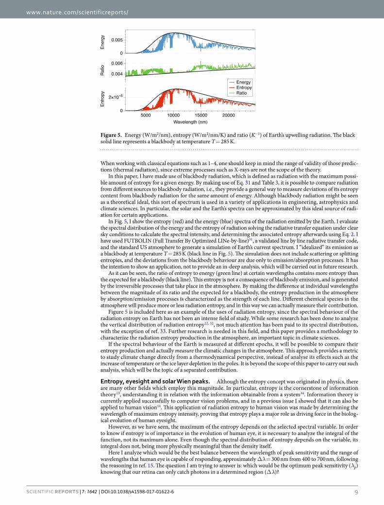
In Fig. 5, I show the entropy (red) and the energy (blue) spectra of the radiation emitted by the Earth. I evaluate the spectral distribution of the energy and the entropy of radiation solving the radiative transfer equation under clear sky conditions to calculate the spectral intensity, and determining the associated entropy afterwards using Eq. 2. I have used FUTBOLIN (Full Transfer By Optimized LINe-by-line)31, a validated line by line radiative transfer code, and the standard US atmosphere to generate a simulation of Earth’s current spectrum. I “idealized” its emission as a blackbody at temperature T = 285 K (black line in Fig. 5). The simulation does not include scattering or splitting entropies, and the deviations from the blackbody behaviour are due only to emission/absorption processes. It has the intention to show an application, not to provide an in-deep analysis, which will be carried out in future research.

As it can be seen, the ratio of entropy to energy (green line) at certain wavelengths contains more entropy than the expected for a blackbody (black line). This entropy is not a consequence of blackbody emission, and is generated by the irreversible processes that take place in the atmosphere. By making the difference at individual wavelengths between the magnitude of its ratio and the expected for a blackbody, the entropy production in the atmosphere by absorption/emission processes is characterized as the strength of each line. Different chemical species in the atmosphere will produce more or less radiation entropy, and in this way we can actually measure their contribution.

Figure 5 is included here as an example of the uses of radiation entropy, since the spectral behaviour of the radiation entropy on Earth has not been an intense field of study. While some research has been done to analyze the vertical distribution of radiation entropy22, 32, not much attention has been paid to its spectral distribution, with the exception of ref. 33. Further research is needed in this field, and this paper provides a methodology to characterize the radiation entropy production in the atmosphere, an important topic in climate sciences.

If the spectral behaviour of the Earth is measured at different epochs, it will be possible to compare their entropy production and actually measure the climatic changes in the atmosphere. This approach provides a metric to study climate change directly from a thermodynamical perspective, instead of analyse its effects such as the increase of temperature or the ice layer depletion in the poles. It is beyond the scope of this paper to carry out such analysis, which will be the topic of a separated contribution.

Entropy, eyesight and solar Wien peaks. Although the entropy concept was originated in physics, there are many other fields which employ this magnitude. In particular, entropy is the cornerstone of information theory13, understanding it in relation with the information obtainable from a system34. Information theory is currently applied successfully to computer vision problems, and in a previous issue I showed that it can also be applied to human vision14. This application of radiation entropy to human vision was made by determining the wavelength of maximum entropy intensity, proving that entropy plays a major role as driving force in the biolog-ical evolution of human eyesight.

However, as we have seen, the maximum of the entropy depends on the selected spectral variable. In order to know if entropy is of importance in the evolution of human eye, it is necessary to analyze the integral of the function, not its maximum alone. Even though the spectral distribution of entropy depends on the variable, its integral does not, being more physically meaningful than the density itself.

Here I analyze which would be the best balance between the wavelength of peak sensitivity and the range of wavelengths that human eye is capable of responding, approximately Δλ = 300 nm from 400 to 700 nm, following the reasoning in ref. 15. The question I am trying to answer is: which would be the optimum peak sensitivity (λp) knowing that our retina can only catch photons in a determined region (Δλ)?

Figure 5. Energy (W/m2/nm), entropy (W/m2/nm/K) and ratio (K−1) of Earth’s upwelling radiation. The black solid line represents a blackbody at temperature T = 285 K.

www.nature.com/scientificreports/

1 0Scientific RepoRts | 7: 1642 | DOI:10.1038/s41598-017-01622-6

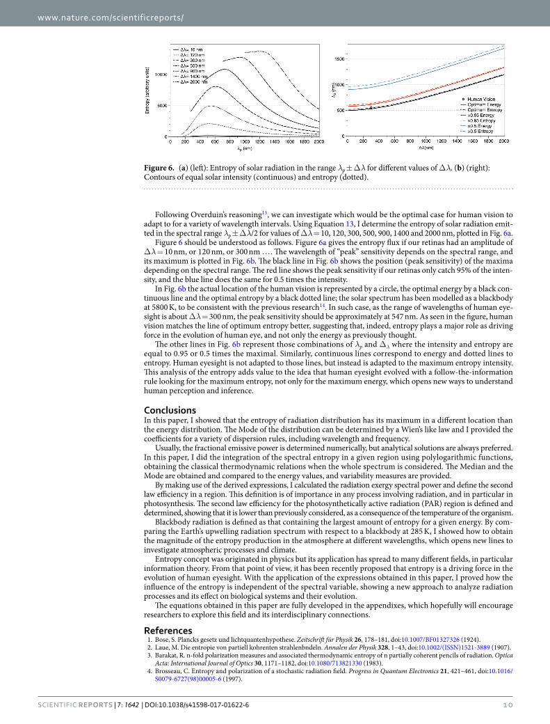
Following Overduin’s reasoning15, we can investigate which would be the optimal case for human vision to adapt to for a variety of wavelength intervals. Using Equation 13, I determine the entropy of solar radiation emit-ted in the spectral range λp ± Δλ/2 for values of Δλ = 10, 120, 300, 500, 900, 1400 and 2000 nm, plotted in Fig. 6a.

Figure 6 should be understood as follows. Figure 6a gives the entropy flux if our retinas had an amplitude of Δλ = 10 nm, or 120 nm, or 300 nm …. The wavelength of “peak” sensitivity depends on the spectral range, and its maximum is plotted in Fig. 6b. The black line in Fig. 6b shows the position (peak sensitivity) of the maxima depending on the spectral range. The red line shows the peak sensitivity if our retinas only catch 95% of the inten-sity, and the blue line does the same for 0.5 times the intensity.

In Fig. 6b the actual location of the human vision is represented by a circle, the optimal energy by a black con-tinuous line and the optimal entropy by a black dotted line; the solar spectrum has been modelled as a blackbody at 5800 K, to be consistent with the previous research14. In such case, as the range of wavelengths of human eye-sight is about Δλ = 300 nm, the peak sensitivity should be approximately at 547 nm. As seen in the figure, human vision matches the line of optimum entropy better, suggesting that, indeed, entropy plays a major role as driving force in the evolution of human eye, and not only the energy as previously thought.

The other lines in Fig. 6b represent those combinations of λp and Δλ where the intensity and entropy are equal to 0.95 or 0.5 times the maximal. Similarly, continuous lines correspond to energy and dotted lines to entropy. Human eyesight is not adapted to those lines, but instead is adapted to the maximum entropy intensity. This analysis of the entropy adds value to the idea that human eyesight evolved with a follow-the-information rule looking for the maximum entropy, not only for the maximum energy, which opens new ways to understand human perception and inference.

ConclusionsIn this paper, I showed that the entropy of radiation distribution has its maximum in a different location than the energy distribution. The Mode of the distribution can be determined by a Wien’s like law and I provided the coefficients for a variety of dispersion rules, including wavelength and frequency.

Usually, the fractional emissive power is determined numerically, but analytical solutions are always preferred. In this paper, I did the integration of the spectral entropy in a given region using polylogarithmic functions, obtaining the classical thermodynamic relations when the whole spectrum is considered. The Median and the Mode are obtained and compared to the energy values, and variability measures are provided.

By making use of the derived expressions, I calculated the radiation exergy spectral power and define the second law efficiency in a region. This definition is of importance in any process involving radiation, and in particular in photosynthesis. The second law efficiency for the photosynthetically active radiation (PAR) region is defined and determined, showing that it is lower than previously considered, as a consequence of the temperature of the organism.

Blackbody radiation is defined as that containing the largest amount of entropy for a given energy. By com-paring the Earth’s upwelling radiation spectrum with respect to a blackbody at 285 K, I showed how to obtain the magnitude of the entropy production in the atmosphere at different wavelengths, which opens new lines to investigate atmospheric processes and climate.

Entropy concept was originated in physics but its application has spread to many different fields, in particular information theory. From that point of view, it has been recently proposed that entropy is a driving force in the evolution of human eyesight. With the application of the expressions obtained in this paper, I proved how the influence of the entropy is independent of the spectral variable, showing a new approach to analyze radiation processes and its effect on biological systems and their evolution.

The equations obtained in this paper are fully developed in the appendixes, which hopefully will encourage researchers to explore this field and its interdisciplinary connections.

References 1. Bose, S. Plancks gesetz und lichtquantenhypothese. Zeitschrift für Physik 26, 178–181, doi:10.1007/BF01327326 (1924). 2. Laue, M. Die entropie von partiell kohrenten strahlenbndeln. Annalen der Physik 328, 1–43, doi:10.1002/(ISSN)1521-3889 (1907). 3. Barakat, R. n-fold polarization measures and associated thermodynamic entropy of n partially coherent pencils of radiation. Optica

Acta: International Journal of Optics 30, 1171–1182, doi:10.1080/713821330 (1983). 4. Brosseau, C. Entropy and polarization of a stochastic radiation field. Progress in Quantum Electronics 21, 421–461, doi:10.1016/

S0079-6727(98)00005-6 (1997).

Figure 6. (a) (left): Entropy of solar radiation in the range λp ± Δλ for different values of Δλ. (b) (right): Contours of equal solar intensity (continuous) and entropy (dotted).

www.nature.com/scientificreports/

1 1Scientific RepoRts | 7: 1642 | DOI:10.1038/s41598-017-01622-6

5. Heald, M. A. Where is the “Wien peak”? American Journal of Physics 71, 1322–1323, doi:10.1119/1.1604387 (2003). 6. Keenan, J. H. Availability and irreversibility in thermodynamics. British Journal of Applied Physics 2, 183–193, doi:10.1088/0508-

3443/2/7/302 (1951). 7. Rant, Z. Exergie, ein neues wort für technische arbeitsfähigkeit. Forschung Ing.-Wesens 22, 36–37 (1956). 8. Petela, R. Exergy of heat radiation. Journal of Heat Transfer 86, 187–192, doi:10.1115/1.3687092 (1964). 9. Rosen, P. Entropy of radiation. Physical Review 96, 555, doi:10.1103/PhysRev.96.555 (1954). 10. Ore, A. Entropy of radiation. Physical Review 98, 887–888, doi:10.1103/PhysRev.98.887 (1955). 11. Landsberg, P. & Tongue, G. Thermodynamics energy conversion efficiencies. Journal of Applied Physics 51, R1–R20,

doi:10.1063/1.328187 (1980). 12. Santillán, M., de Parga, G. A. & Angulo-Brown, F. Black-body radiation and the maximum entropy production regime. European

Journal of Physics 19, 361, doi:10.1088/0143-0807/19/4/008 (1998). 13. Shannon, C. E. A mathematical theory of communication. Bell System Technical Journal 27, 379–423, doi:10.1002/bltj.1948.27.

issue-3 (1948). 14. Delgado-Bonal, A. & Martn-Torres, J. Human vision is determined based on information theory. Scientific Reports 6, 36038,

doi:10.1038/srep36038 (2016). 15. Overduin, J. M. Eyesight and the solar Wien peak. American Journal of Physics 71, 216–219, doi:10.1119/1.1528917 (2003). 16. Planck, M. The Theory of Heat radiation. 1 edn., (P. Blakiston’s Son & Co., Philadelphia, 1913). 17. Einstein, A. Über einen die erzeugung und verwandlung des lichtes betreffenden heuristischen gesichtspunkt. Annalen der Physik

322, 132–148, doi:10.1002/(ISSN)1521-3889 (1905). 18. Stewart, S. A. M. Wien peaks and the Lambert W function. Revista Brasileira de Ensino de Fisica 33, 1–6, doi:10.1590/S1806-

11172011000300008 (2011). 19. Stewart, S. A. M. Spectral peaks and Wien’s displacement law. Journal of Thermophysics and Heat Transfer 26, 689–692, doi:10.2514/1.

T3789 (2012). 20. Stewart, S. A. M. Blackbody radiation functions and polylogarithms. Journal of Quantitative Spectroscopy & Radiative Transfer 113,

232–238 (2012). 21. Wildt, R. Thermodynamics of the gray atmosphere. IV. Entropy transfer and production. Astrophysical Journal 174, 69–77,

doi:10.1086/151469 (1972). 22. Goody, R. & Abdou, W. Reversible and irreversible sources of radiation entropy. Quarterly Journal of the Royal Meteorological Society

122, 483–494, doi:10.1002/(ISSN)1477-870X (1996). 23. Clark, B. A. Computing multigroup radiation integrals using polylogarithm-based methods. Journal of Computational Physics 70,

311–329, doi:10.1016/0021-9991(87)90185-9 (1987). 24. Evans, R. A proof that essergy is the only consistent measure of potential work. Doctoral Thesis, Dartmouth College (1969). 25. Rezac, P. & Metghalchi, H. A brief note on the historical evolution and present state of exergy analysis. International Journal of

Exergy 1, 426–427, doi:10.1504/IJEX.2004.005787 (2000). 26. Liu, L. & Chu, S. X. Radiative exergy transfer equation. Journal of Thermophysics and Heat Transfer 21, 819–822, doi:10.2514/1.31336

(2007). 27. Cloude, S. R. & Pottier, E. Concept of polarization entropy in optical scattering. Optical Engineering 34, 1599–1610,

doi:10.1117/12.202062 (1995). 28. Wijewardane, S. & Goswami, Y. Exergy of partially coherent thermal radiation. Energy 42, 497–502, doi:10.1016/j.energy.2012.03.019

(2012). 29. Candau, Y. On the exergy of radiation. Solar Energy 75, 241–247, doi:10.1016/j.solener.2003.07.012 (2003). 30. Duysens, L. The path of light in photosynthesis. In: The photochemical apparatus. Brookhaven Symposia in Biology 11, 18–25 (1958). 31. Martin-Torres, F. J. & Mlynczak, M. G. Application of FUTBOLIN (FUll Transfer By Ordinary Line-by-Line) to the analysis of the

solar system and extrasolar planetary atmospheres. In AAS/Division for Planetary Sciences Meeting Abstracts #37, vol. 37 of Bulletin of the American Astronomical Society, 1566 (2005).

32. Li, J., Chýlek, P. & Lesins, G. B. Entropy in climate models. Part I: Vertical structure of atmospheric entropy production. Journal of the Atmospheric Sciences 51, 1691–1701 (1994).

33. Stephens, G. L. & Brien, D. M. O. Entropy and climate. I: ERBE observations of the entropy production of the earth. Quarterly Journal of the Royal Meteorological Society 119, 121–152, doi:10.1002/(ISSN)1477-870X (1993).

34. Jaynes, E. T. Information theory and statistical mechanics. Physical Review 106, 620–630, doi:10.1103/PhysRev.106.620 (1957).

AcknowledgementsThe author wants to acknowledge Fundación Iberdrola España for the Fellowship award which partially funded this investigation, and to the family of Prof. José Garmendia Iraundegui for their support and encouragement.

Author ContributionsA.D.-B. is the only author of the manuscript. All the content was originally developed by him for this manuscript.

Additional InformationSupplementary information accompanies this paper at doi:10.1038/s41598-017-01622-6Competing Interests: The author declares that they have no competing interests.Publisher's note: Springer Nature remains neutral with regard to jurisdictional claims in published maps and institutional affiliations.

Open Access This article is licensed under a Creative Commons Attribution 4.0 International License, which permits use, sharing, adaptation, distribution and reproduction in any medium or

format, as long as you give appropriate credit to the original author(s) and the source, provide a link to the Cre-ative Commons license, and indicate if changes were made. The images or other third party material in this article are included in the article’s Creative Commons license, unless indicated otherwise in a credit line to the material. If material is not included in the article’s Creative Commons license and your intended use is not per-mitted by statutory regulation or exceeds the permitted use, you will need to obtain permission directly from the copyright holder. To view a copy of this license, visit http://creativecommons.org/licenses/by/4.0/. © The Author(s) 2017

Entropy of radiation:

the unseen side of lightAlfonso Delgado-Bonal1

1 University of SalamancaInstitute of Fundamental Physics and MathematicsPza. de la Merced S/N, 37008, Salamanca, Spain

alfonso delgado@usal.es

April 24, 2017

Supplementary Information:Appendixes

Contents

Historical development of radiation entropy 2

A Transcendental equation for the Mode 4

B Ratio of normalized entropy to energy 7

C Polylogarithms 9

D Integral of the spectral entropy of radiation 10

E Mean of the energy and entropy of radiation 12

F Higher moments: Variance, Skewness and Kurtosis 14

1

Historical development of radiation entropy

The standard story of the development of the radiation law and the beginning of thequantum theory is usually told in terms of energy, when the reality is that the thermody-namical entropy played the main role in the analysis of radiation. The unfortunate fateof the entropy was to be buried under an unrealistic history about the failure of classicphysics, profound disagreements between theory and experiments and the so called ultra-violet catastrophe; that the energy quanta were then introduced –almost magically– by aprodigious Max Planck, and quantum mechanics became generally accepted immediately.

The truth is that Wien’s law was believed to be correct at the time; only a slightdisagreement was found for long wave radiation, and the Rayleigh-Jeans equation and the“Ultraviolet catastrophe” (named by Ehrenfest in 1911) come across years after Planck’sproposition of his law. The quantum theory and the radiation law were the result of themastering of thermodynamics by Boltzmann, Wien, Planck, Einstein and their contem-poraries.

According to the electromagnetic theory, the energy distribution law was determinedas soon as the entropy S of a linear resonator which interacts with the radiation wereknown as function of the vibrational energy U . Wien was aware of the importance of theentropy [1], and so was Planck.

In October 19th 1900, Max Planck presented in front of the German Physical Societythe law which determines the spectral distribution of blackbody radiation, obtained asan interpolation of Wien’s law [2]. In December 14th 1900 he presented the statisticaljustification of the formula by introducing discrete energy elements, making a novel useof the Boltzmann’s statistical definition of the entropy [3]. The equation leaded to thedevelopment of the quantum theory and it has been vastly studied in the context ofradiative transfer.

At the very end of the XIX century, Wien’s law [4] was proven valid for short wave-lengths but not completely accurate for the whole spectra and, on the other hand, Rayleighhad proposed a formula valid for long wave radiation [5]. From Rayleigh’s formula, therelation between entropy and energy was of the kind:

∂2S

∂2U=

const.

U(1)

The expression on the right-hand side of this functional equation is the change inentropy since n identical processes occur independently, the entropy changes of whichmust simply add up [2].

On the other hand, from Wien’s distribution law the relation would be something ofthe sort:

∂2S

∂2U=

const.

U2(2)

Analyzing a variety of completely arbitrary expressions, Planck proposed the simplestequation (besides the Wien’s one) which yield S as a logarithmic function of U , and

2

coincided with the Wien’s law for small values of U . The logarithmic relation was aconstraint from the probability theory of Mr. Boltzmann, whose works were known byPlanck and were the base upon which the theory was developed afterwards. Withoutfurther justification, Planck included a new term as a series expansion, proportional toU2:

∂2S

∂2U=

const.

U(β + U)(3)

Using this expression and the relation ∂S/∂U = 1/T , one gets a radiation formulawith two constants:

U =C1λ

−5

eC2/λT − 1(4)

By making use of the available data to fit the constants, the equation resulted in thenowadays named Planck’s law.

The formula was, indeed, exact, but it was obtained without any underlying theory,so Planck devoted himself to the task of constructing a radiation theory on the base ofBoltzmann’s statistical mechanics and the logarithmic expression of the entropy:

S = k logW (5)

where S is the thermodynamic entropy, W is the number of possible microstates, and kis Boltzmann’s constant (introduced later by Planck). In a system composed by incoherentradiation beams [6][7], the total entropy can be expressed as the sum S = S1 + S2 whichimplies that:

W = W1 ·W2 (6)

where W is the number of ways in which one can distribute P energy elements overN hypothetical resonators. Using combinatory analysis, Planck obtained the expressionfor the microstates [3], and using the Boltzmann’s entropy expression, he obtained theentropy distribution [8]:

S = k [(N + P ) ln (N + P )−N lnN − P lnP ] (7)

As the aim of Planck was to obtain the energy distribution, he made the marveloushypothesis of discrete energy, ε = hν, motivated by Boltzmann’s works, obtaining theexpression:

S = k

[(1 +

U

hν

)ln

(1 +

U

hν

)− U

hνlnU

hν

](8)

At this point, differentiating with respect to U and using the relation ∂S/∂U = 1/T ,Planck obtained:

1

T=

k

hνln

(1 +

hν

U

)(9)

3

which directly gave him the expression for the energy distribution law that he waslooking for:

U =hν

exp(hν/kT )− 1(10)

With this expression, going back to the entropy, the spectral entropy of radiation is[6]:

Sν =kν2

c2

{(1 +

1

ehνkT − 1

)log

(1 +

1

ehνkT − 1

)− 1

ehνkT − 1

log

(1

ehνkT − 1

)}(11)

This expression was obtained later by many other ways [7][9][10] but, interestingly, theuse of the entropy in the analysis of radiation is mainly forgotten nowadays. However, thesituation was quite different in the past, and several Nobel laureates worked and publishedresearch related directly to the topic, such as Wien [1], Planck [6], Einstein [7], von Laue[11], Lorentz [12] or Kastler [13] among others.

A Transcendental equation for the Mode

The Planck’s law in frequency is:

Lν =2hν3

c21

ehνkT − 1

(12)

The expression for the entropy is more complex, and corresponds to the entropy ofbosons. Prior to the derivative, it is a good idea to manipulate the expression arithmeti-cally, rewriting it as:

Sν =2kν2

c2

{(1 +

1

ehνkT − 1

)log

(1 +

1

ehνkT − 1

)− 1

ehνkT − 1

log

(1

ehνkT − 1

)}=

2kν2

c2· 1

ehνkT − 1

{ehνkT log

(ehνkT

ehνkT − 1

)− log

(1

ehνkT − 1

)}

=2kν2

c2· 1

ehνkT − 1

{ehνkT · log e

hνkT + (e

hνkT − 1) · log

(1

ehνkT − 1

)}=

2kν2

c2· 1

ehνkT − 1

{ehνkThν

kT+ (e

hνkT − 1) · log

(1

ehνkT − 1

)}=

2kν2

c2· hνkT

ehνkT

ehνkT − 1

+2hν2

c2log

(1

ehνkT − 1

)

4

=2hν3

c2T+

2hν3

c2T

1

ehνkT − 1

+2hν2

c2log

(1

ehνkT − 1

)=

2hν3

c2T+

1

T· Lν +

2kν2

c2· log

(1

ehνkT − 1

) (13)

In this way, the second term is the same than in the case of the energy, and thecalculations can be recycled. Doing dS/dν = 0 and removing a factor of 2:

dS

dν=

3hν2

c2T+

3hν2

c2T(ehνkT − 1

) − h2ν3

kT 2c2ehνkT(

ehνkT − 1

)2+

2kν

c· log

(1

ehνkT − 1

)− hν2

c2T

ehνkT(

ehνkT − 1

) = 0

(14)

As in the case of the energy, one can appreciate that frequency corresponds to thedispersion coefficient m = 3, wich will be seen later. Continuing with the derivative,looking for common denominator with the term 1

c2T 2

(ehνkT −1

)2 and manipulating the latest

expression, we have:

dS

dν=

3hν2T(ehνkT − 1

)2c2T 2

(ehνkT − 1

)2 +3hν2T

(ehνkT − 1

)c2T 2

(ehνkT − 1

)2 − h2ν3

kT 2c2ehνkT(

ehνkT − 1

)2+

2kνT 2(ehνkT − 1

)2c2T 2

(ehνkT − 1

)2 · log

(1

ehνkT − 1

)− hν2T

c2T 2

ehνkT

(ehνkT − 1

)(ehνkT − 1

)2 = 0

(15)

From which the numerator must be zero in order to be dS/dν = 0:

dS

dν= 3hν2T

(ehνkT − 1

)2+ 3hν2T

(ehνkT − 1

)− h2ν3

kehνkT

+ 2kνT 2(ehνkT − 1

)2· log

(1

ehνkT − 1

)− hν2Te

hνkT

(ehνkT − 1

)= 0

(16)

Doing the change of variable x = hνkT→ ν = xkT

h, we have:

dS

dν= 3

T 3k2

hx2 (ex − 1)2 + 3

T 3k2

hx2 (ex − 1)− T 3k2

hx3ex

+ 2T 3k2

hx (ex − 1)2 · log

(1

ex − 1

)− T 3k2

hx2ex (ex − 1) = 0

(17)

which getting ride of the factor T 3k2

h·x gives the transcendental equation showed in Eq.

6 in the main text. If the same procedure is followed for the wavelength representation, the

5

result is Eq. 8 in the main text. In the case of choosing the wavelength representation, the“arithmetically transformed” expression for the entropy is shown in the next appendix.

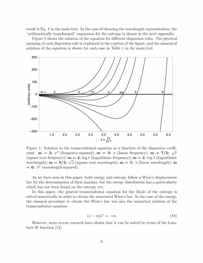
Figure 1 shows the solution of the equation for different dispersion rules. The physicalmeaning of each dispersion rule is explained in the caption of the figure, and the numericalsolution of the equation is shown for each case in Table 1 in the main text.

2 3 7/2 4 9/2 5 6m =

(arb

itrar

y un

its)

−300

−200

−100

0

100

200

300

x = hxλk T

1.5 2.0 2.5 3.0 3.5 4.0 4.5 5.0 5.5 6.0

Figure 1: Solution to the transcendental equation as a function of the dispersion coeffi-cient. m = 2: ν2 (frequency-squared); m = 3: ν (linear frequency); m = 7/2:

√ν

(square root frequency); m = 4: log ν (logarithmic frequency); m = 4: log λ (logarithmicwavelength); m = 9/2:

√λ (square root wavelength); m = 5: λ (linear wavelength); m

= 6: λ2 (wavelength-squared).

As we have seen in this paper, both energy and entropy follow a Wien’s displacementlaw for the determination of their maxima, but the energy distribution has a particularitywhich has not been found on the entropy yet.

In this paper, the general transcendental equation for the Mode of the entropy issolved numerically in order to obtain the associated Wien’s law. In the case of the energy,the classical procedure to obtain the Wien’s law was also the numerical solution of thetranscendental equation:

(x−m)ex = −m (18)

However, more recent research have shown that it can be solved in terms of the Lam-bert W function [14]:

6

benergy =hc/k

m+W0(−me−m)(19)

The details of this function are perfectly described in [15], and provides an elegantanalytical solution to the problem. The general equation obtained in this paper resemblesthe one obtained for the energy, but its solution in terms of Lambert W function is notstraightforward and it is beyond the scope of this paper. Perhaps a skilled reader cansolve it, which will provide an analytical beauty to the problem treated in this section.

B Ratio of normalized entropy to energy

The entropy of radiation distribution in the wavelength representation, as in the previousappendix, can be rewritten as:

Sλ =2kc

λ41

ehc/λkT − 1

{ehc/λkT log

(ehc/λkT

ehc/λkT − 1

)− log

(1

ehc/λkT − 1

)}=

2kc

λ41

ehc/λkT − 1

{ehc/λkT log

(ehc/λkT

)+ (ehc/λkT − 1) log

(1

ehc/λkT − 1

)}=

2kc

λ41

ehc/λkT − 1

{ehc/λkT

hc

λkT+ (ehc/λkT − 1) log

(1

ehc/λkT − 1

)}=

2kc

λ4ehc/λkT

ehc/λkT − 1

hc

λkT+

2kc

λ4log

(1

ehc/λkT − 1

)=

2kc

λ4hc

λkT+

2kc

λ41

ehc/λkT − 1

hc

λkT+

2kc

λ4log

(1

ehc/λkT − 1

)(20)

Which reduces to:

Sλ =2hc2

Tλ5+

1

TLλ +

2kc

λ4· log

(1

ehcλkT − 1

)(21)

The value of the ratio of normalized entropy to energy, n, is determined by the equa-tion:

Sλ/Sλ,maxLλ/Lλ,max

= n (22)

Where Sλ,max and Lλ,max are the maxima of the entropy and the energy respectively.The relation can be rewritten as:

Sλ · Lλ,max = n · Sλ,max · Lλ (23)

Sλ,max and Lλ,max are determined by their corresponding Wien’s laws, so we can usethe relations λmax,energy · T = benergy and λmax,entropy · T = bentropy, expressing the functionsat their maxima as:

7

Sλ,max =2hc2 · T 5

T · b5entropy+

1

T

2hc2

b5entropy

T 5

ehc

kbentropy − 1+

2kc

b4entropy· T 4 · log

(1

ehc

kbentropy − 1

)(24)

Lλ,max =2hc2

b5energy

T 5

ehc

kbenergy − 1(25)

For simplicity, calling c1 = 2hc2, c2 = hc/k and c3 = 2kc, the relation described inEquation 23 leads to the equation:

c1T · λ5

· c1b5energy

T 5

(ec2/benergy − 1)+

1

T

c1λ5

1

(ec2/λT − 1)

c1b5energy

T 5

(ec2/benergy − 1)

+c3λ4· log

(1

ec2/λT − 1

)· c1b5energy

T 5

(ec2/benergy − 1)=

n ·{c1T

T 5

b5entropy· c1λ5

1

(ec2/λT − 1)+

1

T

c1b5entropy

T 5

(ec2/bentropy − 1)

c1λ5

1

(ec2/λT − 1)

+c3

b4entropy· T 4 · log

(1

ec2/bentropy − 1

)· c1λ5

1

(ec2/λT − 1)

}(26)

Removing T 4

λ5, naming x = c2

λTand multiplying both sides by (ex − 1), the equation is

reduced to:

ex +ex − 1

x· log

(1

ex − 1

)= n ·

{(benergybentropy

)5

·(e

hckbenergy − 1

)·{

1 +1

ehc

kbentropy − 1+kbentropyhc

· log

(1

ehc

kbentropy − 1

)}} (27)

The right side of the equation depends only on the value of the ratio, since the terminside the curl is a constant of an approximate value of 1.204196. Using this value, theequation is approximated to:

ex +ex − 1

x· log

(1

ex − 1

)= n · 1.204196 (28)

The solution for different values of the ratio is shown in Table 3 of the main text. Forexample, for a value or ratio equal to unity, the numerical solution of the transcendentalequation is x = 4.878482. Undoing the change of variable, we have:

λn=1T =hc

k · 4.8784820= 2.94923 · 10−3m K (29)

8

C Polylogarithms

Detailed information of polylogarithms –an old function known since 250 years ago [16]–can be found for example in [17]. In this appendix the most important properties whichare of interest for this work are reviewed.

The polylogarithm is a special function Lis(z) of order s and argument z. For specialvalues of s the polylogarithm is reduced to an elementary function (such as the naturallogarithm). Polylogarithms are defined as the infinite sum for arbitrary complex order sand for all complex arguments z [18]:

Lis(z) =∞∑k=1

zk

ks= z +

z2

2s+z3

3s+ . . . (30)

or as the repeated integral of itself:

Lis+1(z) =

∫ z

0

Lis(t)

tdt (31)

The derivatives follow from the defining power series in Equation 30, and particularlyfor exponential functions:

z∂Lis(z)

∂z= Lis−1(z)

∂Lis(ex)

∂x= Lis−1(e

x)

∂Lis(e−x)

∂x= −Lis−1(e−x)

(32)

In the special case s = 1, the polylogarithm is reduced to the ordinary natural loga-rithm:

Li1(z) = − log(1− z) (33)

for s = 0, -1, -2, the polylogarithm is:

Li0(z) =z

1− z; Li−1(z) =

z

(1− z)2; Li−2(z) =

z(1 + z)

(1− z)3 (34)

Some properties of the integral of exponential functions are listed here. FollowingEquation 31, we have: ∫ ∞

x

Lis(e−t)dt = Lis+1(e

−x) (35)

and the indefinite integral with an arbitrary constant:

9

∫Lis(e

−x)dx = −Lis+1(e−x) (36)

Particularly interesting are the integrals of the form [19]:∫xkLi0(e

−x)dx = −k∑

n=0

xk−nLin+1(e−x)

Γ(k + 1)

Γ(k + 1− n)(37)

where k is a non-negative integer and Γ(x) is the Euler gamma function.For z = 1 the polylogarithm reduces to the Riemann zeta function:

Lis(1) = ζ(s), (Re(s) > 1) (38)

D Integral of the spectral entropy of radiation

Using Equation 21 the integral is reduced to three simpler integrals:∫Sλdλ =

∫2hc2

Tλ5dλ+

∫1

TLλdλ+

∫2kc

λ4· log

(1

ehcλkT − 1

)dλ (39)

In the following I will do the change of variable hcλkT

= x→ − hcλ2kT

dλ = dx. The threeintegrals are solved separately, named i), ii) and iii) respectively. Integral i) is reducedto:

∫2hc2

Tλ5dλ =

∫2hc2

Tλ5−kThc

λ2dx =

∫−2kc

λ3dx =

∫−2kc

k3T 3

h3c3x3dx =

−2k4T 3

h3c2x4

4(40)

Integral ii) is the same integral than in the case of the energy. It is solved using therelation in Equation 37 with k = 3:

∫1

TLλdλ =

1

T

∫2hc2

λ51

ehcλkT − 1

dλ =1

T

∫2hc2

λ51

ehcλkT − 1

−kThc

λ2dx

=1

T

−2k4T 4

h3c2

∫x3

1

ex − 1dx =

−2k4T 3

h3c2

∫x3

e−x

1− e−xdx

=−2k4T 3

h3c2

∫x3Li0(e

−x)dx

=−2k4T 3

h3c2

(−

k=3∑n=0

xk−nLin+1(e−x)

Γ(k + 1)

Γ(k + 1− n)

)

=2k4T 3

h3c2(x3Li1(e

−x) + 3x2Li2(e−x) + 6xLi3(e

−x) + 6Li4(e−x))

(41)

10

Let’s solve now integral iii). Although there are many ways to solve it, the simplestway is by making use of the relation between the logarithm and polylogarithms, i.e., using

the fact that Li1(x) =∞∑k=1

xk

k= − log(1− x):

iii)

∫2kc

λ4log

(1

ehcλkT − 1

)dλ =

−2k4T 3

h3c2

∫x2 log

(1

ex − 1

)dx

=−2k4T 3

h3c2

∫x2 log

(e−x

1− e−x

)dx

=−2k4T 3

h3c2

{∫x2 log

(e−x)dx−

∫x2 log

(1− e−x

)dx

}=−2k4T 3

h3c2

{−x

4

4−∫x2(−Li1(e−x)

)dx

}(42)

The latest integral can solved doing integration by parts and knowing the proper-ties of the polylogarithms. In particular, I will use the derivative property (Eq. 32),d

dx

[Li1(e

−x)]

= −Li0(e−x), and the same summation relation used before (Eq. 37):

iii)−2k4T 3

h3c2

{−x

4

4+

∫x2Li1(e

−x)dx

}=−2k4T 3

h3c2

{−x

4

4+x3

3Li1(e

−x)−∫x3

3

(−Li0(e−x)

)dx

}=−2k4T 3

h3c2

{−x

4

4+x3

3Li1(e

−x) +1

3

(−

k=3∑n=0

xk−nLin+1(e−x)

Γ(k + 1)

Γ(k + 1− n)

)} (43)

Once the three integrals are completed, they can be put together, which reduces to

(note: the sum expression is typed as:(−∑k=3

n=0 . . .)

= −{x3Li1(e−x) + 3x2Li2(e−x)

+6xLi3(e−x) + 6Li4(e

−x)} ):

∫Sxdx =

−2k4T 3

h3c2

{x4

4+

(−

k=3∑n=0

. . .

)− x4

4+x3

3Li1(e

−x) +1

3

(−

k=3∑n=0

. . .

)}

=−2k4T 3

h3c2

{x3

3Li1(e

−x) +4

3

(−

k=3∑n=0

. . .

)}

=−2k4T 3

h3c2

{x3

3Li1(e

−x)− 4

3

(x3Li1(e

−x) + 3x2Li2(e−x) + 6xLi3(e

−x) + 6Li4(e−x))}

=2k4T 3

h3c2{x3Li1(e

−x) + 4x2Li2(e−x) + 8xLi3(e

−x) + 8Li4(e−x)}

(44)

11

For isotropic radiation (radiant intensity is independent of direction), the monochro-matic flux density is Fλ = π Lλ, and the same accounts for the entropy. Multiplying the

previous equation by π, and using the Stefan’s constant σ =2π5k4

15h3c2:

=S =15

π4σT 3

{x3Li1(e

−x) + 4x2Li2(e−x) + 8xLi3(e

−x) + 8Li4(e−x)}

(45)

When the whole spectrum is considered, the polylogarithmic term is reduced to8ζ(8) = 4π4

45, and the obtained entropy flux density is:

=S =15

π4σT 3

(4π4

45

)=

4

3σT 3

(46)

in agreement with the thermodynamic theory [6].

E Mean of the energy and entropy of radiation

The Mean of the normalized distribution in the x variable is determined as:∫x · Sxdx =

45

4π4

{∫x4dx+

∫x4

1

ex − 1dx+

∫x3 log

(1

ex − 1

)dx

}(47)

In order to obtain the value of the integral, it will be divided into two parts. The first

part,

∫x4

1

ex − 1dx is the one with elements similar to the energy and will be named i),

and the second part will be the rest of it, named ii). Although one can think that it wouldbe simpler to do each integral separately, the third integral (the one with the logarithm)is not convergent and cannot be solved alone. However, the introduction of the x4 factorreduces its complexity and makes it integrable, as it will be seen below.

The integral of the first part, i.e. the energy term i), is called Bose-Einstein integral,and its expression is, in general:

I(p) =

∫ ∞0

xp−1

ex − 1dx (48)

Using series expansion:1

1− e−x=∞∑k=0

(e−x)k (49)

the integral is:

12

∫ ∞0

xp−1

ex − 1dx =

∫ ∞0

e−x1

(1− e−x)xp−1dx =

∫ ∞0

e−x

[∞∑k=0

(e−x)k

]xp−1dx

=∞∑k=0

∫ ∞0

e−(k+1)xxp−1dx

(50)

Doing the change of variable:

(k + 1)x = y → dx =dy

k + 1(51)

the integral is reduced to:

∞∑k=0

∫ ∞0

e−(k+1)xxp−1dx =∞∑k=0

1

(k + 1)p

∫ ∞0

yp−1e−ydy = Γ(p)∞∑k=1

1

(k)p= Γ(p)ζ(p)

(52)where Γ(p) is the Euler gamma function and ζ(p) is the Riemann zeta function. The

reader should notice the change in the k index in the final steps of the previous equation.In this particular case p = 5, and the Bose-Einstein integral is then reduced to

Γ(5)ζ(5). Therefore:

i)45

4π4

∫ ∞0

x41

ex − 1dx =

45

4π4[24 · ζ(5)] (53)

This result is also applicable to the case of the energy, although the pre-factor wouldbe 15/π4 instead of 45/4π4. The Mean of the energy of radiation in the x variable is:

Lmean =15

π4[24 · ζ(5)] ' 3.83223 (54)

which in the λT variable is ' 3.75447 (× 106 nm K).Continuing with the entropy, the other terms, i.e. integral ii), are integrated like in

the previous appendix, using the properties of the polylogarithms:

ii)45

4π4

∫ {x4 + x3 log

(1

ex − 1

)}dx =

45

4π4

∫ {x4 + x3 log

(e−x

1− e−x

)}dx

=45

4π4

∫ {x4 + x3 log

(e−x)− x3 log

(1− e−x

)}dx

=45

4π4

∫ {x4 + x3(−x)− x3 log

(1− e−x

)}dx =

45

4π4

∫ {x3Li1(e

−x)}dx

=45

4π4

{x4

4Li1(e

−x)−∫x4

4(−Li0(e−x))dx

}

13

=45

4π4

{x4

4Li1(e

−x)− 1

4

(k=4∑n=0

x4−nLin+1(e−x)

Γ(4 + 1)

Γ(4 + 1− n)

)}=

45

4π4

{−x3Li2(e−x)− 3x2Li3(e

−x)− 6xLi4(e−x)− 6Li5(e

−x)} (55)

With the intention to evaluate the solution in 0 and ∞, it is useful to know someproperties of the polylogarithms. For the argument equal to unity, the polylogarithm isreduced to the Riemann Zeta function, Lis(1) = ζ(s) (Equation 38). In this case, whenthe value of x is zero (or equivalently, the product λT is equal to ∞), the argument ise−x = e−0 = 1.

On the other hand, using L’Hopital rule recursively it can be proved that [19]:

limx→∞

x4−nLin+1(e−x) = 0, n = 0,1,2,3,4 (56)

With all this, equation ii) evaluated in [0,∞) is reduced to:

ii)45

4π4

∫ {x4 + x3 log

(1

ex − 1

)}dx =

45

4π4

[6Li5(e

0)]

=45

4π4[6ζ(5)] (57)

Thus, the total value of the Mean in the x variable is i) + ii):∫ ∞0

x · Sxdx =45

4π4[6ζ(5) + 24ζ(5)] =

45

4π4[30ζ(5)] ' 3.59272 (58)

In the λT variable, the Mean is ' 4.00477 (× 106 nm K).

F Higher moments: Variance, Skewness and Kurto-

sis

In this section, I will calculate the moments of the distribution until the fourth order,following the very same formalism than in the previous appendix.

The moment of order one corresponds to the Mean, which has been calculated before:

E[x] =45

4π4· 30 · ζ(5) ' 3.59272 (59)

The moment of order two is calculated as:

E[x2] =

∫x2 · Sxdx =

45

4π4

{∫x5dx+

∫x5

1

ex − 1dx+

∫x4 log

(1

ex − 1

)dx

}(60)

Doing the splitting of the integrals as we did in Appendix E, the order of the Bose-

Einstein integral is now p = 6, being i)

∫ ∞0

x51

ex − 1dx = Γ(6)ζ(6) = 120ζ(6).

14

The rest of the integral is reduced, using the properties of polylogarithms applied inEq. 55, to:

ii)45

4π4

{−x4Li2(e−x)− 4x3Li3(e

−x)− 12x2Li4(e−x)− 24xLi5(e

−x)− 24Li6(e−x)}(61)

Reasoning as before, in the [0,∞) interval the integral is evaluated as ii) 24ζ(6), andthe moment E[x2] = i) + ii) is:

E[x2] =45

4π4· [120ζ(6) + 24ζ(6)] =

45

4π4· 144 · ζ(6) ' 16.9193 (62)

The order three is similarly calculated as:

E[x3] =

∫x3 · Sxdx =

45

4π4

{∫x6dx+

∫x6

1

ex − 1dx+

∫x5 log

(1

ex − 1

)dx

}(63)

where now the Bose-Einstein integral is Γ(7)ζ(7) = 720ζ(7), and the rest of the integralis reduced to:

ii)45

4π4

{−x5Li2(e−x)− 5x4Li3(e

−x)− 20x3Li4(e−x)− 60x2Li5(e

−x)

−120xLi6(e−x)− 120Li7(e

−x)} (64)

and therefore:

E[x3] =45

4π4· [720ζ(7) + 120ζ(7)] =

45

4π4· 840 · ζ(7) ' 97.8235 (65)

Finally, for the moment of order 4, the Bose-Einstein integral is Γ(8)ζ(8) = 5040ζ(7)and the rest of the integral is:

ii)45

4π4

{−x6Li2(e−x)− 6x5Li3(e

−x)− 30x4Li4(e−x)− 120x3Li5(e

−x)

−360x2Li6(e−x)− 720xLi7(e

−x)− 720Li8(e−x)} (66)

which gives a final value of:

E[x4] =45

4π4· [5040ζ(8) + 720ζ(8)] =

45

4π4· 5760 · ζ(8) ' 667.948 (67)

In general, the moment of order n can be determined as:

E[xn] =45

4π4

[4 + n

4 + n− 1Γ(4 + n)ζ(4 + n)

], n ≥ 1 (68)

15

References

[1] Wien, W. Temperatur und entropie der strahlung. Annalen der Physik 288, 132–165(1894).

[2] Planck, M. Uber eine Verbesserung der Wienschen Spektral Gleichung. Verhandl.Dtsch. phys. Ges. 2 (1900).

[3] Planck, M. On the Theory of the Energy Distribution Law of the Normal Spectrum.Verhandl. Dtsch. phys. Ges. 2 (1900).

[4] Wien, W. Ueber die energievertheilung im emissionsspectrum eines schwarzenkorpers. Annalen der Physik 294, 662–669 (1896).

[5] Rayleigh, L. LIII. Remarks upon the law of complete radiation. Philosophical Mag-azine. Series 5 49, 539 (1900).

[6] Planck, M. The Theory of Heat radiation (P. Blakiston’s Son & Co., Philadelphia,1913), 1 edn.

[7] Einstein, A. Uber einen die erzeugung und verwandlung des lichtes betreffendenheuristischen gesichtspunkt. Annalen der Physik 322, 132–148 (1905).

[8] Planck, M. Ueber das Gesetz der Energieverteilung im Normalspectrum. Annalender Physik 309, 553–563 (1901).

[9] Bose, S. Plancks gesetz und lichtquantenhypothese. Zeitschrift fur Physik 26, 178–181 (1924).

[10] Rosen, P. Entropy of radiation. Physical Review 96, 555 (1954).

[11] Laue, M. Die entropie von partiell kohrenten strahlenbndeln. Annalen der Physik328, 1–43 (1907).

[12] Lorentz, H. The Theory of Radiation and the Second Law of Thermodynamics.KNAW, Proceedings 3, 436–450 (1901).

[13] Kastler, A. Radiation and entropy, coherence and negentropy. In Haken, H. (ed.)Synergetics, vol. 2 of Springer Series in Synergetics, 18–25 (Springer Berlin Heidel-berg, 1977).

[14] Valluri, S. R., Jeffrey, D. J. & Corless, R. M. Some applications of the Lambert Wfunction to physics. Canadian Journal of Physics 78, 823–831 (2000).

[15] Corless, R. M., Gonnet, G. H., Hare, D. E. G., Jeffrey, D. J. & Knuth, D. E. On theLambert W function. Advances in Computational Mathematics 5, 329–359.

[16] Olver, F. W. J., Lozier, D. W., Boisvert, R. F. & Clark, C. W. NIST handbook ofmathematical functions (Cambridge University Press, Cambridge, 2010), 1 edn.

16

[17] Apostol, T. M. Polylogarithm. In Olver, F. W. J., Lozier, D. M., Boisvert, R. F. &Clark, C. W. (eds.) NIST Handbook of Mathematical Functions (Cambridge Univer-sity Press, 2010).

[18] Abramowitz, M. & Stegun, I. A. Handbook of Mathematical Functions with Formulas,Graphs, and Mathematical Tables (Dover Publications, New York, 1972).

[19] Stewart, S. A. M. Blackbody radiation functions and polylogarithms. Journal ofQuantitative Spectroscopy & Radiative Transfer 113, 232 – 238 (2012).

17

View publication statsView publication stats