Entropy and MDL discretization of continuous variables for ...sci2s.ugr.es/keel/pdf/specific/articulo/IJIS00.pdf · Entropy and MDL Discretization of Continuous Variables for

Entropy and MDL Discretization ofContinuous Variables for BayesianBelief NetworksEllis J. Clarke,* Bruce A. BartonMaryland Medical Research Institute, 600 Wyndhurst Ave.,Baltimore, Maryland 21210

An efficient algorithm for partitioning the range of a continuous variable to a discreteŽ .number of intervals, for use in the construction of Bayesian belief networks BBNs , is

presented here. The partitioning minimizes the information loss, relative to the numberof intervals used to represent the variable. Partitioning can be done prior to BBNconstruction or extended for repartitioning during construction. Prior partitioning allows

Ž .either Bayesian or minimum descriptive length MDL metrics to be used to guide BBNconstruction. Dynamic repartitioning, during BBN construction, is done with a MDLmetric to guide construction. The methods are demonstrated with data from twoepidemiological studies and these results are compared for all of the methods. The use ofthe partitioning algorithm resulted in more sparsely connected BBNs, than with binarypartitioning, with little information loss from mapping continuous variables into discreteones. Q 2000 John Wiley & Sons, Inc.

I. INTRODUCTION

In the course of conducting clinical trials or epidemiological studies, a largeamount of data may be collected. Often, exploratory data analysis is done to getan indication of the interactions of many study variables. This process is not anexhaustive data analysis, but allows the construction of a model of the interac-tions between study variables to guide further analysis.

Ž .This paper develops a general method for exploratory data analysis EDAfor medical studies, which provides a common scaling for all types of variables.One of the major problems in this context is combining nominal, discrete, andcontinuous variables in the same model. The following sections develop this

Ž .theme, using Bayesian belief networks BBNs , and emphasize methods toconvert continuous variables to discrete ones. New methods for discretization ofcontinuous variables, based upon information theory, are presented here. Also,

*Author to whom correspondence should be addressed.

Ž .INTERNATIONAL JOURNAL OF INTELLIGENT SYSTEMS, VOL. 15, 61]92 2000Q 2000 John Wiley & Sons, Inc. CCC 0884-8173r00r010061-32

CLARKE AND BARTON62

these methods are applied using either a Bayesian or a minimum descriptiveŽ .length MDL metric to guide the discretization and the results are compared.

Pearl presents a Bayesian method for constructing a probabilistic networkfrom a database of records.1,2 The network can provide insight into the proba-bilistic dependencies that exist among the variables in a database. The computerprogram searches for a network structure that has a high posterior probability,given the database, and outputs its structure and its probability. A Bayesian

Ž .belief structure is a directed acyclic graph DAG in which nodes representdomain variables and arcs between nodes represent probabilistic dependencies.Variables may be continuous or discrete. The representation of conditionaldependencies and independencies is an essential function of a belief network.The belief structure is augmented by conditional probabilities to form a Bayesianbelief network. For each node in a belief network, there is a conditional-prob-

Ž .ability function that relates this node to its immediate predecessors parents .In order to develop a general method using BBNs for exploratory data

analysis in large medical study databases with continuous measurements, thecharacteristics of the continuous variable frequency distributions can be empiri-cally used to preprocess the data and to augment BBN construction. This isdone to simplify and to clarify the network structure for a given database.

An efficient new algorithm is presented to partition the value range of acontinuous random variable. This algorithm uses the characteristics of the

Ž .information content entropy of the continuous variable for the partitioningand does not require comparison with another variable, as do previous methods.Test results show that BBNs, constructed from continuous variables discretizedby this algorithm, demonstrate stronger dependencies than comparable BBNswith equal interval partitioning.

The method used above for entropy based discretization is extended todynamically repartition a continuous variable’s values in relation to anothervariable. An information theoretic metric, which guides BBN construction, isused to guide the repartitioning. BBNs constructed in this way show stronger,and more unexpected, dependencies among variables than those constructedwith only entropy partitioning.

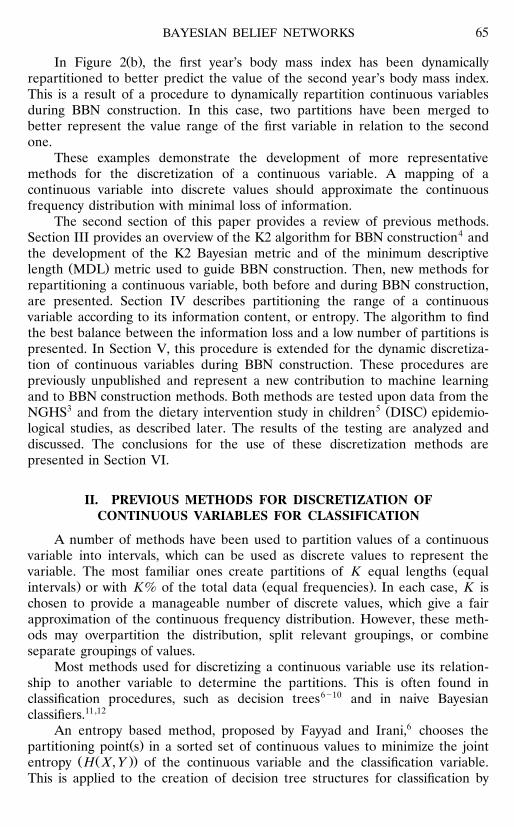
3 Ž .A continuous variable from the NHLBI growth and health study NGHSstudy is used to briefly illustrate these methods. The variable is the first year’sbody mass index measurement. The original continuous frequency distribution is

Ž .shown in Figure 1 a , accompanied by the discrete distribution resulting frombinary equal interval partitioning. The split point for the partitioning is shownon the original distribution.

A better partitioning of the continuous distribution uses equal frequencyŽ .intervals, which are quintiles in the example in Figure 1 b . However, the

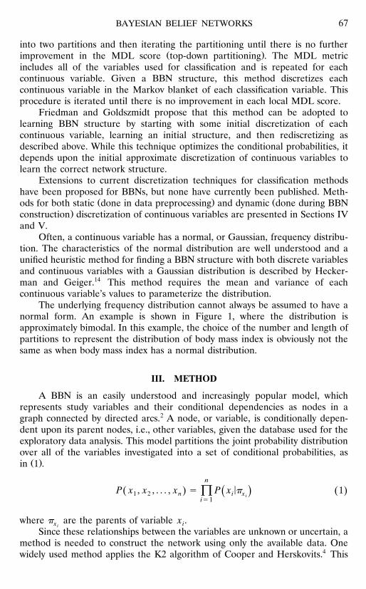
resulting uniform distribution is not representative of the original one.The algorithm for entropy discretization was used to partition the continu-

Ž .ous distribution in Figure 2 a . Here, the intervals are of varying lengths andfrequencies to minimize the information loss due to discretization. The discrete

Ž .distribution, in Figure 2 a , gives a very good approximation of the originaldistribution.

BAYESIAN BELIEF NETWORKS 63

Ž.

Fig

ure

1.N

GH

Sfir

stye

arbo

dym

ass

inde

x.O

rigi

nal

dist

ribu

tion

and

equa

lin

terv

alor

freq

uenc

ypa

rtiti

onin

g.a

Ž.

Bin

ary

part

ition

ing,

bqu

intil

epa

rtiti

onin

g.

CLARKE AND BARTON64

Ž.

Fig

ure

2.N

GH

Sfir

stye

arbo

dym

ass

inde

x.O

rigi

nal

dist

ribu

tion

and

entr

opy

ordy

nam

icM

DL

part

ition

ing.

aŽ.

Ent

ropy

base

dpa

rtiti

onin

g,b

dyna

mic

MD

Lba

sed

part

ition

ing

inre

latio

nto

seco

ndye

arB

MI.


Ž .In Figure 2 b , the first year’s body mass index has been dynamicallyrepartitioned to better predict the value of the second year’s body mass index.This is a result of a procedure to dynamically repartition continuous variablesduring BBN construction. In this case, two partitions have been merged tobetter represent the value range of the first variable in relation to the secondone.

These examples demonstrate the development of more representativemethods for the discretization of a continuous variable. A mapping of acontinuous variable into discrete values should approximate the continuousfrequency distribution with minimal loss of information.

The second section of this paper provides a review of previous methods.Section III provides an overview of the K2 algorithm for BBN construction4 andthe development of the K2 Bayesian metric and of the minimum descriptive

Ž .length MDL metric used to guide BBN construction. Then, new methods forrepartitioning a continuous variable, both before and during BBN construction,are presented. Section IV describes partitioning the range of a continuousvariable according to its information content, or entropy. The algorithm to findthe best balance between the information loss and a low number of partitions ispresented. In Section V, this procedure is extended for the dynamic discretiza-tion of continuous variables during BBN construction. These procedures arepreviously unpublished and represent a new contribution to machine learningand to BBN construction methods. Both methods are tested upon data from the

3 5 Ž .NGHS and from the dietary intervention study in children DISC epidemio-logical studies, as described later. The results of the testing are analyzed anddiscussed. The conclusions for the use of these discretization methods arepresented in Section VI.

II. PREVIOUS METHODS FOR DISCRETIZATION OFCONTINUOUS VARIABLES FOR CLASSIFICATION

A number of methods have been used to partition values of a continuousvariable into intervals, which can be used as discrete values to represent the

Žvariable. The most familiar ones create partitions of K equal lengths equal. Ž .intervals or with K% of the total data equal frequencies . In each case, K is

chosen to provide a manageable number of discrete values, which give a fairapproximation of the continuous frequency distribution. However, these meth-ods may overpartition the distribution, split relevant groupings, or combineseparate groupings of values.

Most methods used for discretizing a continuous variable use its relation-ship to another variable to determine the partitions. This is often found inclassification procedures, such as decision trees6 ] 10 and in naive Bayesianclassifiers.11,12

An entropy based method, proposed by Fayyad and Irani,6 chooses theŽ .partitioning point s in a sorted set of continuous values to minimize the joint

Ž Ž ..entropy H X, Y of the continuous variable and the classification variable.This is applied to the creation of decision tree structures for classification by

CLARKE AND BARTON66

Ž .recursively finding more partitioning points top-down discretization . Themethod is expanded to minimize a MDL metric to choose the partitioningpoints.

Another MDL based method for discretization is described by Pfahringer.7

A set of the best partitioning points is determined by recursively partitioning theŽ D .sorted variable values to a depth D 2 y 1 partitions in a binary tree. Then

the MDL metric is used in a best first search in this set to determine the bestpartitions for decision tree classification.

A method that merges adjacent partitions of sorted variable values, accord-ing to the x 2 statistical test, is described by Liu and Setiono.8 The variablevalues are sorted and initially partitioned into, at most, N intervals. Theintervals are first recursively merged according to the lowest x 2 value until asignificance level of 0.05 is reached for each partition. The intervals are furthermerged until a preset error rate with the classification variable is reached. Ifthere is only one resulting interval, the variable is not relevant to the classifica-tion problem and is dropped. This method combines the discretization ofcontinuous variables with feature selection for classification.

Dougherty, Kohavi, and Sahami9 compared several discretization tech-niques with decision trees and with naive Bayesian classifiers. They found that aMDL metric, similar to that used by Fayyad and Irani,6 provided slightly betterclassifications in both methods.

A metric for discretization, based upon a variable’s classification in relationto other variables, is described by Hong.10 This metric is based upon a Knearest neighbor clustering technique and is used to generate decision trees. Aninteresting feature of this method is that it returns an optimal number ofpartitions according to the metric. This is done by finding the ‘‘knee’’ of theplotted curve of the score as a function of the number of partitions. The plot is aconcave function of the metric; the knee is the point on the plot where the

Ž .changes in the number of variable values X axis become greater thanŽ .the changes in the metric value Y axis . The concavity of a plot is exploited in

the information theoretic discretization methods developed in Section IV.Subramonian, Venkata, and Chen,13 describe a visual framework for inter-

active discretization for decision tree classification. A user can choose betweenseveral algorithms and metrics for a classification problem, instead of beinglimited to one method and metric. The choice of metrics includes cross-entropyand the L y 1 norm between two distributions.

Pazzani11 describes a technique for iterative discretization of continuousvariables for naive Bayesian classifiers. Each continuous variable is initiallydivided into five partitions. For each variable, two partitions are then merged ora partition is divided into two partitions to find a lower classification error. Thisprocedure is repeated for each continuous variable until the error rate can nolonger be reduced.

Another method for constructing naive Bayesian classifiers using a MDLmetric is presented by Friedman and Goldszmidt.12 This method begins byfinding the best initial partition of a continuous variable by dividing the range


into two partitions and then iterating the partitioning until there is no furtherŽ .improvement in the MDL score top-down partitioning . The MDL metric

includes all of the variables used for classification and is repeated for eachcontinuous variable. Given a BBN structure, this method discretizes eachcontinuous variable in the Markov blanket of each classification variable. Thisprocedure is iterated until there is no improvement in each local MDL score.

Friedman and Goldszmidt propose that this method can be adopted tolearning BBN structure by starting with some initial discretization of eachcontinuous variable, learning an initial structure, and then rediscretizing asdescribed above. While this technique optimizes the conditional probabilities, itdepends upon the initial approximate discretization of continuous variables tolearn the correct network structure.

Extensions to current discretization techniques for classification methodshave been proposed for BBNs, but none have currently been published. Meth-

Ž . Žods for both static done in data preprocessing and dynamic done during BBN.construction discretization of continuous variables are presented in Sections IV

and V.Often, a continuous variable has a normal, or Gaussian, frequency distribu-

tion. The characteristics of the normal distribution are well understood and aunified heuristic method for finding a BBN structure with both discrete variablesand continuous variables with a Gaussian distribution is described by Hecker-man and Geiger.14 This method requires the mean and variance of eachcontinuous variable’s values to parameterize the distribution.

The underlying frequency distribution cannot always be assumed to have anormal form. An example is shown in Figure 1, where the distribution isapproximately bimodal. In this example, the choice of the number and length ofpartitions to represent the distribution of body mass index is obviously not thesame as when body mass index has a normal distribution.

III. METHOD

A BBN is an easily understood and increasingly popular model, whichrepresents study variables and their conditional dependencies as nodes in agraph connected by directed arcs.2 A node, or variable, is conditionally depen-dent upon its parent nodes, i.e., other variables, given the database used for theexploratory data analysis. This model partitions the joint probability distributionover all of the variables investigated into a set of conditional probabilities, as

Ž .in 1 .

n

<P x , x , . . . , x s P x p 1Ž . Ž .Ž .Ł1 2 n i x iis1

where p are the parents of variable x .x ii

Since these relationships between the variables are unknown or uncertain, amethod is needed to construct the network using only the available data. Onewidely used method applies the K2 algorithm of Cooper and Herskovits.4 This

CLARKE AND BARTON68

algorithm, and many similar ones,15 ] 17 requires all of the variables to havediscrete values. Continuous variables can be transformed into discrete ones bypartitioning the range of values into intervals of equal case frequencies, e.g.,quartiles,18 or into equal interval lengths. However, partitions of equal casefrequencies are represented as a uniform distribution of variable values in theBBN node, which may not be representative of the underlying continuousfrequency distribution of the variable values.

A heuristic method to find the number of equal length partitions, whichprovides a good mapping of continuous variables to discrete ones for construct-ing a BBN, is used for comparison with heuristic methods used to find varyinglength partitions. This method uses either the K2 metric4 or the minimum

Ž . 17descriptive length MDL metric to select the number of partitions, which bestapproximates the underlying probability distribution of a continuously valuedvariable, to be used in constructing a BBN.

A. Modified K2 Algorithm

The original K2 algorithm, proposed by Cooper and Herskovits,4 uses aBayesian measure to pick the most probable parents of each discrete variablefrom the variable’s predecessors in a completely ordered list. Each variable isrepresented by a node in the BBN.

The basic algorithm used here is essentially the same as K2, but with twomodifications. First, a partially ordered list of variables is used. This ordering isbased upon a temporal ordering of measurement variables, with measurementstaken at the same time placed at the same level in the ordering. Only nodesfrom preceding levels can be considered as parents of a particular node.

ŽThe second modification is the discretization of continuous nodes varia-.bles during the search for the parents of each node, as described in Section V.

This discretization is done to find the best partitioning of a continuous node’svalue range. The partitions result in discrete values, which may maximize theevaluation metric for this node as a parent. This partitioning is done in relationto the child node and its current set of parents.

The metric used for the K2 algorithm by Cooper and Herskovits,4 is basedupon the theorem for describing the joint probability of a BBN structure, B ,s

given a database, D. Thus

q rn i ir y 1 !Ž .iP B , D s P B N ! 2Ž . Ž . Ž .Ł Ý Łs s i jkN q r y 1 !Ž .is1 ks1i j ijs1

Ž .where i refers to the ith variable x , n is the number of variables, q is the seti i

of instantiations the parents, p , of variable x can have, r is the set of valuesi i i

variable x can have, N is the number of cases with the kth of the r values ofi i jk i


x and the jth of the q combination of values of the parents of x , andi i i

ri

N s NÝi j i jkks1

Ž .This theorem is based upon four assumptions: 1 all variables have discreteŽ . Ž .values; 2 database cases occur independently; 3 there are no missing values;

Ž .and 4 the prior probabilities of all database structures are uniform.Ž .The K2 metric, which is derived from 2 , is used to find a maximally

probable set of parents of a variable, based upon the set of conditionalprobabilities for this structure found from the given data. The metric is

q ri ir y 1 !Ž .ig i , p s N ! 3Ž . Ž .Ł Łi i jkN q r y 1 !Ž .js1 ks1i j i

This is used by the K2 algorithm in a greedy search to find the set of parents ofa variable which maximizes the metric’s value. Its value is approximatelyproportional to the probability of each conditional probability distribution, for anode and its parents, in a Dirichlet distribution. The metric value for a node isinitialized for the variable by itself, independent of other variables. This is usedas a starting point for the discretizing of continuous variables here.

The K2 metric, given a uniform probability distribution on a variable, givesw Ž . Ž .xa greater value for a smaller number of partitions r in 2 and 3 than fori

more partitions. As the number of partitions decreases, the ŁN ! increases ati jkŽ .a faster rate than the N q r y 1 ! term. This results in a higher metric scorei j i

for fewer partitions of a uniform distribution. In general, the K2 metric favorsfewer partitions of a variable, given the same data.

B. MDL Encoding for a BBN

The MDL19,20 encoding of a BBN combines a measure of the underlyingprobability distributions of the data sample with a measure of the networkcomplexity. Both of these measures are proportional to the information contentof the BBN, in bits. The minimum of the sum of these measures describes aBBN which closely models the underlying data but is not excessively complex.Smaller conditional dependencies between variables, as described in the previ-ous section, will usually not be represented in a BBN induced from the datausing the MDL encoding.

The MDL measure of a BBN maximizes the probability of the networkstructure while minimizing the network complexity. It makes a tradeoff betweenextreme accuracy, which may be specific to the data sample used for construc-tion, and the BBN model usefulness. The MDL measure minimizes the sum ofthe encoding lengths, in bits, of both the data and the BBN model. However,finding the network which exactly minimizes these two sums is computationallyintractable. Therefore, search heuristics are used which find a low, but notnecessarily minimum, MDL encoding. The problem is reduced to using mea-

CLARKE AND BARTON70

sures that are proportional to the MDL encoding instead of measuring theabsolute value of the encoding.

Ž .To represent a particular BBN, it is necessary and sufficient to have a aŽ .list of parents of each node and b the set of conditional probabilities associ-

ated with each node.Ž .The descriptive length needed to encode these items is L B , D , where Bs s

is a BBN structure and D is the database. It is defined by Bouckaert17 as

1L B , D s log P B y N ? H B , D y k log N 4Ž . Ž . Ž . Ž .s 2 s s 22

Ž . Ž .where N is the number of cases, as in 2 , H B , D is the mutual informationsbetween a node and its parents over all nodes, and k is the cost of encoding the

Ž .table of conditional probabilities between a node and its parents. H B , D issdefined as

q rn i i N Ni jk i jky log 5Ž .Ý Ý Ý 2N Ni jis1 js1 ks1

Ž .where i refers to the ith variable x , n is the number of variables, q is the seti iof values the parents of variable x can have, r is the set of values variable xi i ican have, N is the number of cases with the k th value of x and the jthi jk icombination of values of the parents of x , andi

ri

N s NÝi j i jkks1

Ž . Ž .as in 2 . H B , D increases as arcs are added to a network structure, since qs iincreases with each parent node, indicated by an arc.

Ž .The k value in 4 is defined as

n

r y 1 r 6Ž . Ž .Ý Łi jx gpis1 j i

This term increases when arcs are added, since more conditional probabilitiesŽ .are needed for each parent node x g p .j i

Ž .The descriptive length equation 4 shows that highly connected networksrequire longer encodings. Therefore, the MDL principle tends to favor networks

Ž .in which the nodes have a smaller number of parents less connected and inwhich nodes taking on a large number of values are not parents of nodes thatalso have a large number of values. This encoding scheme generates a prefer-ence for more efficient networks. Since the encoding length of a model isincluded in the descriptive length, a preference for networks that require thestorage of fewer probability parameters is enforced.

Ž .The a priori probability of a network structure, P B , is assumed to besequal to any other one when there is no prior information, so it is dropped fromthe metric. The K2 Bayesian metric makes the same assumption.


Ž .The MDL measure defined in 4 is similar to the one defined by Lam and16 ŽBacchus. However, their algorithm searches a separate space of possible BBN.structures for each network with the same number of connected nodes to find a

BBN structure.The final MDL metric used by Bouckaert,17 for finding the local network of

a single node and its parents, is reduced to

q ri i N 1i jkm i , p s N log y q ? r y 1 log N 7Ž . Ž . Ž .Ý Ýi i jk 2 i i 2N 2i jjs1 ks1

Ž . Ž . Ž .This is derived from Eq. 4 . The first term of 4 is dropped because P B issassumed to be equal for all networks, as mentioned above. The first group of

Ž .terms, in 7 , is the conditional entropy between a node and its parents. This isŽ .derived from the second group of terms in 4 . The N in these terms does not

change, so it is dropped. The conditional entropy, for a node and its parents, isproportional to the joint entropy.21 The second group is the number of bitsneeded to encode the conditional probability table for the node, which is a

Ž .restatement of 6 . The metric is maximized in the heuristic search, since theusual negation in conditional entropy is reversed.

The metric used by Lam and Bacchus16 is based upon the mutual informa-tion between a node and its parents in a network.22 Since mutual information

Ž . Ž . Ž < . Ž .can be defined as I X ; Y s H X y H X Y and H X does not change, theŽ < . Ž .negated conditional entropy yH X Y is proportional to I X ; Y .

C. Test Data for Discretization Method

A data sample of 704 cases was selected from a subset of an epidemiologi-cal health study database to demonstrate this method. The sample is from theNHLBI Growth and Health Study,3 a study of the development of obesity inyoung black and white girls. It is not representative of the overall study datasince cases selected had no missing values and the data were selected tospecifically demonstrate the described method. The variables selected were raceŽ . Ž .categorical; range 1, 2 , maturation stage categorical; range 1]6 , Quetelet

Ž .index, a measure of body mass continuous , average daily caloric intakeŽ . Ž .continuous , measurement age continuous , and a psychological test measure-

Ž .ment of self worth categorical; range 1]4 . The girls were 9 or 10 years of ageat the first measurement. All variables used in this analysis, except race, wererepeatedly measured over 5 years, with age being the age at each year’smeasurement.

Another data sample of 466 cases was chosen from another epidemiologicaldatabase for demonstration. This sample is from the Dietary Intervention Studyin Children,5 a clinical trial designed to assess the efficacy of a lipid loweringdiet in 8]10 year old children. The sample is not representative of the overallstudy, since cases selected had no missing values. One treatment group receivedseveral sessions to teach the children and their parents the benefits and menusof a low-fat diet. The other group received only general dietary information.

CLARKE AND BARTON72

Ž . ŽThe variables chosen were gender categorical; range 1, 2 , treatment cate-. Ž . Žgorical; range 1, 2 , total cholesterol level continuous , body mass index con-

. Ž . Ž .tinuous , triglycerides continuous , activity level categorical; range 1]6 , andŽ .measurement age continuous . Except for gender and treatment, all variables

were repeatedly measured at the child’s entrance into the study, after 12, 36,and 60 months; again age is the child’s age at each measurement.

The modified K2 algorithm was implemented in the SASQIML program-ming language on an IBM RS6355 workstation. SAS was used since the studydata analysis is done in this environment. This language is interpretive, so theCPU times were excessive. Much shorter execution times would be expectedusing a compiled language.

IV. ENTROPY BASED DISCRETIZATION OF CONTINUOUSVARIABLES BEFORE BBN CONSTRUCTION

As mentioned above, most methods used for discretizing a continuousvariable use its relationship to another variable to determine the partitions. Themethod proposed here is used to partition a continuous variable by itself. It isbased on finding an ‘‘optimal’’ discretization by minimizing both the loss ofinformation or entropy and the number of partitions. This procedure can beused in a variety of machine learning and data mining problems, which requirediscretization of a continuous variable.

A. Entropy Properties of a Continuous Variable

Initially, the range of a continuous variable, from a database sample, isdivided into intervals which contain at least one case each. This is done after

Ž Ž ..sorting on the variable values. At most, there would be m intervals O m forŽ .m cases. This converts the continuous variable into a discrete one, with O m

values.Entropy, or information, is maximized when the frequency]probability

distribution has the maximum number of values.21 Since there is a discretepartition for every distinct value in the continuous distribution in the database,there is no information or entropy loss from the database sample.

The entropy of a discrete random variable X is defined as

H X s y p x log p x 8Ž . Ž . Ž . Ž .Ý 2xgX

Ž .This can also be written as H p .21 Ž .Cover and Thomas define a function f x to be convex over an interval

Ž . Ž .a, b if for every x , x in a, b and 0 F l F 1,1 2

f l x q 1 y l x F l f x q 1 y l f x 9Ž . Ž . Ž . Ž . Ž .Ž .1 2 1 2

A function f is concave if yf is convex. Examples of convex and concaveŽ . 21functions are shown in Figure 3. H p is proven to be a concave function of p.

These definitions are applied in the following lemmas.


Ž . Ž .Figure 3. Examples of convex a and concave b functions.

LEMMA 4.1. Let each distinct älue of a continuous random äriable X, in thecase database, be represented by a separate inter̈ al. Let the number of inter̈ als be

Ž .k, 1 F k F m for m cases. Let the probability of X in each inter̈ al be p i ,Ž .1 F i F k. Let the entropy of the distribution of k discrete inter̈ als be H p . If twok

Ž . Ž .adjacent inter̈ als, i, i q 1, are chosen such that H p y H p is minimized,k ky1Ž Ž . Ž ..then the change in the probability of the combined inter̈ al, p i q p i q 1 , is

monotonically nondecreasing.

Ž . Ž .Proof. To minimize H p y H p , i and i q 1 are chosen such that thek ky1Ž . Ž . Ž .sum p i q p i q 1 is minimized. The minimum values of p i are set at the

initial partitioning of intervals for each distinct value of X. As adjacent intervalsare merged, the difference between adjacent interval probabilities can only

Ž .increase or remain the same. Therefore, the change in each combined p i ismonotonically nondecreasing. B

LEMMA 4.2. If X is a continuous random äriable, in the case database, with kŽ . Ž .distinct älues 1 F k F m with an inter̈ al for each distinct älue, then H p is ak

concaë function oër k, when each decrease in the number of inter̈ als is chosen toŽ .minimize the change in H p .k

Proof. The maximum entropy of a sorted continuous random variable, in aŽ .database of m cases, is the entropy H p when each distinct value is repre-

sented by a separate interval.Starting at the point of maximum entropy and maximum number of k

Ž .intervals 2 F k F m , the two adjacent intervals are merged which result in theŽ . Ž . Ž .smallest change in H p to give H p . This smallest change in H pk ky1 k

results from merging the two adjacent intervals with the smallest differenceŽ . Ž .between p i and p i q 1 . If this procedure is applied repeatedly, the size of

this sum is monotonically nondecreasing.

CLARKE AND BARTON74

Ž . Ž .Since H p is a concave function of p, H p is a concave function of pk kŽ .in this procedure. Since each p represents k intervals in this procedure, H pk k

is a concave function of the number of decreasing intervals when the p iskmonotonically nondecreasing. B

The procedure of merging adjacent intervals, described above, is continueduntil a stopping point is reached. The determination of this point is describednext.

Ž .As seen in Figure 3 b , a concave function, such as entropy, is monotoni-cally increasing with an increase in X. However, its rate of increase is alwaysdecreasing as it approaches the maximum value of X. The entropy over allpartitionings of the NGHS variable year 2 body mass index is shown in Figure 4.

As stated above, the maximum entropy occurs with the maximum numberof partitions. The best tradeoff between maximum information and a manage-able number of partitions is reached when the change in X becomes greaterthan the change in the entropy of X. This is at the knee of the function plot.

If a chord is drawn from the origin of the graph to the point of maximumentropy and number of partitions, all of the points on the concave function plotwill be above the chord. The change in X becomes greater than the change inthe entropy of X at the point on the curve which is furthest from the chord.This is displayed as the vertical line from the chord to the curve in Figure 4.

The maximum height of a point on the function curve above the chord isproportional to x y y y x. Therefore, the stopping point for the merging ofmax maxadjacent intervals is reached just before the decrease in this score. A similarmethod for determining discretization intervals relative to a classification vari-able, using a metric based upon a sum of squares distance, is described by

Figure 4. Entropy over all partitionings of NGHS variable year 2 body mass index.Chord shown with perpendicular line to indicate optimal number of partitions.


Hong.10 However, this method, as well as all of the others referenced here,bases discretization upon one variable’s relationship to another. Also, it makesno use of the entropy measure.

Repeatedly merging adjacent intervals, as described above, gives the leastdecrease in entropy and allows intervals with low frequency difference to bemerged prior to those with higher frequency differences. This method preservesobvious groupings or clusters.

B. Discretization Procedure

This entropy discretization method was applied to the continuous variablesin both the NGHS and DISC datasets. For each continuous variable in adataset, the dataset was sorted on that variable and only the values of thatvariable were input to the program.

The two adjacent values with the smallest entropy difference were foundand merged. If there was more than one pair of adjacent values with thesmallest entropy difference, one pair was randomly chosen. This procedure wasiterated until the stopping criteria, finding the knee of the concave function plot,

Žwas met. The initial variable values, which defined the partitions the split.points , were then stored. After every continuous variable was partitioned in this

manner, the stored split points were written to an output file.The procedure is implemented in the following algorithm:

1. procedure ENTD;2. r* Input: a database, D, of m cases and n continuous variables;

Output: a file of partition split points for every continuous variable; *r3. for i s 1 to n do; r* do for each continuous variable *r4. sort D by continuous variable i;5. read m cases of variable i into array X ;6. accumulate frequency counts and save split points for each distinct k values

of X ;7. oldent s entropy of X with k partitions;8. initent s oldent;9. init k s k;

10. oldchek s 0;11. oktogo s TRUE;

Ž .12. while oktogo ; r* loop to find knee of entropy curve *r13. find the 2 adjacent intervals, a, a q 1, with the minimum frequency differ-

ence;14. merge intervals a, a q 1;

Ž .15. newent s entropy of X with intervals a, a q 1, merged k y 1 partitions ;Ž . Ž Ž .. Ž .16. newchek s initk) newent y initent) k y 1 ; r* calculate max x y

Ž .ymax y x *rŽ .17. if newchek ) oldchek r* check to continue *rthen do;

18. reset split points for X to reflect merger of a, a q 1;19. reset interval frequencies;20. oldent s newent;21. k s k y 1;

CLARKE AND BARTON76

22. oldchek s newchek;23. end;24. else oktogo s FALSE;25. end while;26. save split points for X ;27. end i loop;28. output to file split points for all continuous variables;29. end ENTD.

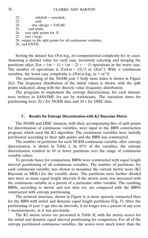
Ž .Sorting the dataset has O m log m computational complexity for m cases.2Assuming a distinct value for each case, iteratively selecting and merging the

Ž Ž . Ž . .partitions takes 2 m q m y 1 q m y 2 q ??? 1 operations in the worst case.Ž Ž .. Ž 2 .The number of operations is 2 m m y 1 r2 or O m . With n continuous

Ž Ž 2 ..variables, the worst case complexity is O n m log m q m .2The partitioning of the NGHS year 1 body mass index is shown in Figure

Ž .2 a . The frequency distribution of the initial values is shown, with the splitpoints indicated, along with the discrete value frequency distribution.

The programs to implement the entropy discretization, for each dataset,were written in SASQIML for use by statisticians. The execution times forpartitioning were 20 s for NGHS data and 10 s for DISC data.

C. Results for Entropy Discretization with K2 Bayesian Metric

The NGHS and DISC datasets, with their accompanying files of split pointsfor discretization of continuous variables, were input to the BBN constructionprogram, which used the K2 algorithm. The continuous variables were initiallypartitioned according to their split points and the BBN was constructed.

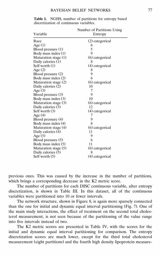
The number of partitions for each NGHS continuous variable, after entropydiscretization, is shown in Table I. In 85% of the variables, the entropydiscretization resulted in 10 or fewer partitions over the range of continuousvariable values.

To provide bases for comparison, BBNs were constructed with equal lengthinterval partitioning of all continuous variables. The number of partitions, for

Žeach continuous variable, was chosen to maximize the current metric score K2.Bayesian or MDL for the variable alone. The partitions were further divided

into twice as many equal length intervals if the metric score was increased withthe continuous variable as a parent of a particular other variable. The resultingBBNs, according to metric and test data set, are compared with the BBNsconstructed with entropy partitioning.

The network structure, shown in Figure 6, is more sparsely connected thenŽ .for the BBN with initial and dynamic equal length partitions Fig. 5 . After the

partitioning of year 1 age into six intervals, it no longer was a parent of any year1 measurements, as it was previously.

The K2 metric scores are presented in Table II, with the metric scores forthe initial and dynamic equal interval partitioning for comparison. For all of theentropy partitioned continuous variables, the scores were much lower than the


Table I. NGHS, number of partitions for entropy baseddiscretization of continuous variables.

Number of Partitions UsingVariable Entropy

Ž .Race 2 categoricalŽ .Age 1 6

Ž .Blood pressure 1 5Ž .Body mass index 1 9Ž . Ž .Maturation stage 1 6 categorical

Ž .Daily calories 1 8Ž . Ž .Self worth 1 4 categorical

Ž .Age 2 8Ž .Blood pressure 2 9Ž .Body mass index 2 6Ž . Ž .Maturation stage 2 6 categorical

Ž .Daily calories 2 10Ž .Age 3 7



Ž .Age 4 7Ž .Blood pressure 4 9Ž .Body mass index 4 8Ž . Ž .Maturation stage 4 6 categorical

Ž .Daily calories 4 11Ž .Age 5 9



previous ones. This was caused by the increase in the number of partitions,which brings a corresponding decrease in the K2 metric score.

The number of partitions for each DISC continuous variable, after entropydiscretization, is shown in Table III. In this dataset, all of the continuousvariables were partitioned into 10 or fewer intervals.

The network structure, shown in Figure 8, is again more sparsely connectedŽ .than the one for initial and dynamic equal interval partitioning Fig. 7 . One of

the main study interactions, the effect of treatment on the second total choles-terol measurement, is not seen because of the partitioning of the value rangeinto five intervals instead of two.

The K2 metric scores are presented in Table IV, with the scores for theinitial and dynamic equal interval partitioning for comparison. The entropydiscretization scores are much lower, except for the third total cholesterol

Ž .measurement eight partitions and the fourth high density lipoprotein measure-

CLARKE AND BARTON78

Figure 5. NGHS network, K2 Bayesian metric, with all continuous variables initiallyŽ .partitioned into two equal length intervals year 5 blood pressure three intervals .

Dynamically repartitioned into equal length intervals, as indicated by numbers adjacentto directed arcs.

Figure 6. NGHS network, K2 Bayesian metric, with all continuous variables initiallypartitioned using entropy.


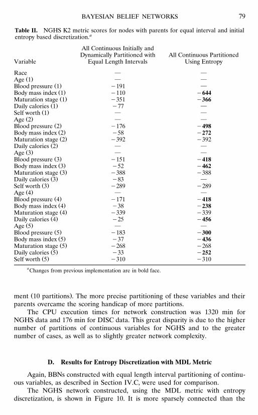
Table II. NGHS K2 metric scores for nodes with parents for equal interval and initialaentropy based discretization.

All Continuous Initially andDynamically Partitioned with All Continuous Partitioned

Variable Equal Length Intervals Using Entropy

Race } }Ž .Age 1 } }

Ž .Blood pressure 1 y191 }Ž .Body mass index 1 y110 y644Ž .Maturation stage 1 y351 y366

Ž .Daily calories 1 y77 }Ž .Self worth 1 } }

Ž .Age 2 } }Ž .Blood pressure 2 y176 y498Ž .Body mass index 2 y58 y272Ž .Maturation stage 2 y392 y392

Ž .Daily calories 2 } }Ž .Age 3 } }

Ž .Blood pressure 3 y151 y418Ž .Body mass index 3 y52 y462Ž .Maturation stage 3 y388 y388

Ž .Daily calories 3 y83 }Ž .Self worth 3 y289 y289

Ž .Age 4 } }Ž .Blood pressure 4 y171 y418Ž .Body mass index 4 y38 y238Ž .Maturation stage 4 y339 y339

Ž .Daily calories 4 y25 y456Ž .Age 5 } }

Ž .Blood pressure 5 y183 y300Ž .Body mass index 5 y37 y436Ž .Maturation stage 5 y268 y268

Ž .Daily calories 5 y33 y252Ž .Self worth 5 y310 y310

aChanges from previous implementation are in bold face.

Ž .ment 10 partitions . The more precise partitioning of these variables and theirparents overcame the scoring handicap of more partitions.

The CPU execution times for network construction was 1320 min forNGHS data and 176 min for DISC data. This great disparity is due to the highernumber of partitions of continuous variables for NGHS and to the greaternumber of cases, as well as to slightly greater network complexity.

D. Results for Entropy Discretization with MDL Metric

Again, BBNs constructed with equal length interval partitioning of continu-ous variables, as described in Section IV.C, were used for comparison.

The NGHS network constructed, using the MDL metric with entropydiscretization, is shown in Figure 10. It is more sparsely connected than the

CLARKE AND BARTON80

Table III. DISC, number of partitions for entropy baseddiscretization of continuous variables.

Number of Partitions UsingVariable Entropy

Ž .Gender 2 categoricalŽ .Treatment 2 categorical

Ž .Age 1 8Ž .Total cholesterol 1 2

Ž .High density lipoprotein 1 4Ž .Triglycerides 1 8

Ž .Body mass index 1 6Ž . Ž .Activity level 1 5 categorical










Figure 7. DISC network, K2 Bayesian metric, with all continuous variables initiallypartitioned into two equal length intervals. Dynamically repartitioned into equal lengthintervals, as indicated by numbers adjacent to directed arcs.


Figure 8. DISC network, K2 Bayesian metric, with all continuous variables initiallypartitioned using entropy method.

Ž .BBN with initial and dynamic equal interval partitioning Fig. 9 . Major differ-ences are the lack of year to year dependencies in blood pressure measurementsand maturation stage being the only race dependency.

The MDL metric scores are presented in the middle column of Table V,with the scores of initial and dynamic equal interval partitioning for comparison.The scores are much lower, due to the greater number of partitions.

The network constructed, with entropy discretization of DISC data, isshown in Figure 12. It has almost half of the dependencies shown for continuousvariables, compared to the BBN for initial and dynamic equal length interval

Ž .partitions Fig. 11 . Most of the missing connections are for triglyceride mea-surements, which are completely independent in this implementation.

The MDL metric scores are presented in the middle column of Table VI,with the initial and dynamic equal interval partitioning scores for comparison.All of the scores are much lower, except for the third total cholesterol measure-ment and the fourth high density lipoprotein measurement. This decrease in theMDL scores is consistent with the decrease in the K2 metric scores for thesevariables.

The CPU execution time for network construction was 468 min for NGHSdata and 97 min for DISC data. These execution times for each dataset isroughly proportional to the times using the K2 metric.

E. Discussion of Results

The entropy discretization method provides an optimal balance betweeninformation loss and a manageable number of values for continuous variables.Also, it can be done efficiently without comparison to another variable. In the

CLARKE AND BARTON82

Table IV. DISC K2 metric scores for nodes with parents for equal interval and initialaentropy based discretization.

All ContinuousInitially and

Dynamically Partitioned All Continuouswith Equal Partitioned

Variable Length Intervals Using Entropy

Gender } }Treatment } }

Ž .Age 1 } }Ž .Total cholesterol 1 y134 }

Ž .High density lipoprotein 1 } }Ž .Triglycerides 1 } }

Ž .Body mass index 1 } }Ž .Activity level 1 } }

Ž .Age 2 } }Ž .Total cholesterol 2 y122 }

Ž .High density lipoprotein 2 y78 y199Ž .Triglycerides 2 y59 y391

Ž .Body mass index 2 y23 y191Ž .Activity level 2 y226 y226

Ž .Age 3 } }Ž .Total cholesterol 3 y122 y39



Ž .Age 4 } }Ž .Total cholesterol 4 y20 y357




two datasets used for testing, there were generally 10 or fewer partitions used torepresent the value range of a continuous variable.

The increased number of partitions led to more sparsely connected net-works than those with equal length partitions for both the NGHS and DISCdatasets. The number of dependencies shown, involving continuous variables,was nearly halved for both datasets. Also, the higher number of partitionsusually resulted in lower metric scores, as well as increased execution times fornetwork construction.

This method of discretization of continuous variables brings out thestrongest conditional dependencies in the data. These dependencies are strongersince they exist through a more precise partitioning of data value ranges, thanfor equal length interval partitioning.


Figure 9. NGHS network, MDL metric, with all continuous variables initially parti-Ž .tioned into two equal length intervals year 5 blood pressure three intervals . Dynamically

repartitioned into equal length intervals, as indicated by numbers adjacent to directedarcs.

Figure 10. NGHS network, MDL metric, with all continuous variables initially parti-tioned using the entropy method.

CLARKE AND BARTON84

Table V. NGHS MDL metric scores for nodes with parents for equal length intervalaand entropy based discretization.

All ContinuousInitially and All ContinuousDynamically All Continuous Partitioned Using

Partitioned with Partitioned Entropy; DynamicallyEqual Length Using Repartitioned

Variable Intervals Entropy Using MDL

Race } } }Ž .Age 1 } } }

Ž .Blood pressure 1 y637 } }Ž .Body mass index 1 y367 } }Ž .Maturation stage 1 y1221 y1222 y1222

Ž .Daily calories 1 } } }Ž .Self worth 1 } } }

Ž .Age 2 } } }Ž .Blood pressure 2 y591 } }Ž .Body mass index 2 y191 y953 y935Ž .Maturation stage 2 y1359 y1359 y1359

Ž .Daily calories 2 } } }Ž .Age 3 } } }

Ž .Blood pressure 3 y518 } }Ž .Body mass index 3 y175 y1642 y1620Ž .Maturation stage 3 y1340 y1340 y1340

Ž .Daily calories 3 y289 } }Ž .Self worth 3 y980 y980 y980

Ž .Age 4 } } }Ž .Blood pressure 4 y585 } y1277Ž .Body mass index 4 y134 y879 y861Ž .Maturation stage 4 y1165 y1165 y1165

Ž .Daily calories 4 y82 y1832 y1752Ž .Age 5 } } }

Ž .Blood pressure 5 y618 y1068 y1031Ž .Body mass index 5 y121 y1698 y1667Ž .Maturation stage 5 y928 y928 y928

Ž .Daily calories 5 y133 y1000 y974Ž .Self worth 5 y1053 y1053 y1053


V. DYNAMIC REPARTITIONING FOR BBNS BASEDON THE MDL METRIC

A. Introduction

To further improve the accuracy of the BBNs constructed using entropybased discretization of continuous variables, a method for dynamic repartition-ing using the MDL metric was developed. Since higher metric scores result from

Ž .fewer variable values partitions and the initial discretization was not done inrelation to any other variables, this repartitioning merged existing partitions ofcontinuous variables to find more definitive conditional dependencies. This


Figure 11. DISC network, MDL metric, with all continuous variables initially parti-tioned into two equal length intervals. Dynamically repartitioned into equal lengthintervals, as indicated by numbers adjacent to directed arcs.

procedure for dynamically repartitioning continuous variables during BBN con-struction, using the MDL metric, is completely new. It could have wide use indata mining applications using BBN models.

23 Ž .Bouckaert has shown that the MDL metric used here, Eq. 7 , is aconcave function in the number of partitions used in the conditional dependen-

Figure 12. DISC network, MDL metric, with all continuous variables initially parti-tioned using entropy method.

CLARKE AND BARTON86

Table VI. DISC MDL metric scores for nodes with parents for equal interval andaentropy based discretization.

All Continuous All ContinuousInitially and Partitioned UsingDynamically Entropy;

Partitioned with All Continuous DynamicallyEqual Length Partitioned Repartitioned

Variable Intervals Using Entropy Using MDL

Gender } } }Treatment } } }

Ž .Age 1 } } }Ž .Total cholesterol 1 } } }

Ž .High density lipoprotein 1 } } }Ž .Triglycerides 1 } } }

Ž .Body mass index 1 } } }Ž .Activity level 1 } } }

Ž .Age 2 } } }Ž .Total cholesterol 2 y407 } }

Ž .High density lipoprotein 2 y264 y680 y673Ž .Triglycerides 2 y200 } }

Ž .Body mass index 2 y76 y685 y673Ž .Activity level 2 y787 y787 y787

Ž .Age 3 } } }Ž .Total cholesterol 3 y409 y140 y136

Ž .High density lipoprotein 3 y203 y853 y864Ž .Triglycerides 3 y56 } }


Ž .Age 4 } } }Ž .Total cholesterol 4 y66 y1220 y1220

Ž .High density lipoprotein 4 y265 y37 y47Ž .Triglycerides 4 y92 } y1332



cies between parent and child nodes. This is based upon the concavity of theconditional entropy used in the metric. Finding the knee of this function wasused as a stopping point for merging the partitions of continuous variables. Thiswas done by a method similar to the one used to stop the entropy basedpartitioning of a single continuous variable. As described in Section IV.A, theknee of the plot of the concave function is used as a stopping point for mergingpartitions.

If there were no stopping points for mergers, all continuous variables wouldreach a binary partitioning. This is a result of the MDL metric giving a higherscore to variables with fewer values. Two values were the minimum for ameasurement to remain a variable and not to become a constant.


B. Method

As the set of parents of a variable was being found during BBN construc-tion, each continuous variable was dynamically repartitioned to find the highestMDL metric for this variable as a parent. If a continuous variable was beingconsidered as a parent, the two adjacent partitions with the lowest frequencyŽ .probability difference were merged. After this merging, a new MDL metricvalue was found which used this variable, the child variable, and any otherpreviously established parent variables. The merging, of the adjacent partitionswith the lowest frequency difference, was based upon the heuristic that adjacentvariable values, with very similar frequencies, belong to the same value clusterfor predicting the value of another variable.

This merging was iterated until the knee of the MDL function was reached.The resulting metric score was considered to be the best possible for thiscontinuous variable and was used for selecting it as a parent variable. If thevariable was not chosen as a parent, it retained its initial partitioning.

After the child variable and its parents were written to the output file, acontinuous parent variable reverted to its initial partitioning. In this way, eachdynamic repartitioning was independent of any others for the same variable andthe partitioning of the parent as a child node remained unchanged. In thenetwork structure, a new node can be created between the original node and thechild to represent this repartitioning. This new node is a direct parent of thischild node and only of this one child node.

C. Procedure

As described in Section IV.B, the NGHS or DISC dataset, with its accom-panying file of continuous variable split points, was read into the program withthe basic K2 BBN construction algorithm. As each continuous variable wasconsidered as a parent, it was repartitioned, as described above, to find the bestpartitioning relative to a child variable. If the continuous variable was selectedas a parent, it was listed in the output file as one, along with its current splitpoints and the number of partitions. The partitioning of a continuous variablewas always reset after it was considered as a parent. This procedure was used ina modified version of the K2 algorithm, with the repartitioning done accordingby merging the adjacent partitions with the lowest frequency difference, insteadof in the manner of the repartition function in the algorithm.

Aside from the complexity of the initial entropy discretization of the data,this method of dynamic discretization significantly adds to the computationalcomplexity of the K2 based algorithm. With m cases, n variables, r values for a

wŽ . ŽŽ . .variable, and a maximum of c parents, this method uses c rm q r y 1 mŽ .x ŽŽ Ž . . .q ??? 2m operations in the worst case. This comes to O r r y 1 r2 cm or

Ž 2 .O r cm operations for each variable. When combined with the initial complex-Ž 4 .ity for the K2 algorithm of O mn r , this gives a worst case complexity of

Ž 2 4 3 .O m n r c .

CLARKE AND BARTON88

D. Results for Dynamic Repartitioning with the MDL Metric

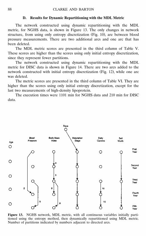
The network constructed using dynamic repartitioning with the MDLmetric, for NGHS data, is shown in Figure 13. The only changes in network

Ž .structure, from using only entropy discretization Fig. 10 , are between bloodpressure measurements. There are two additional arcs and one arc that hasbeen deleted.

The MDL metric scores are presented in the third column of Table V.These scores are higher than the scores using only initial entropy discretization,since they represent fewer partitions.

The network constructed using dynamic repartitioning with the MDLmetric for DISC data is shown in Figure 14. There are two arcs added to the

Ž .network constructed with initial entropy discretization Fig. 12 , while one arcwas deleted.

The metric scores are presented in the third column of Table VI. They arehigher than the scores using only initial entropy discretization, except for thelast two measurements of high-density lipoprotein.

The execution times were 1101 min for NGHS data and 210 min for DISCdata.

Figure 13. NGHS network, MDL metric, with all continuous variables initially parti-tioned using the entropy method, then dynamically repartitioned using MDL metric.Number of partitions indicated by numbers adjacent to directed arcs.


Figure 14. DISC network, MDL metric, with all continuous variables initially parti-tioned using the entropy method, then dynamically repartitioned using MDL metric.Number of partitions indicated by numbers adjacent to directed arcs.

E. Discussion

The dynamic discretization of continuous variables, using the MDL metric,resulted in minor changes in BBN structure. However, metric scores weregenerally higher and additional dependencies were found.

The use of dynamic repartitioning, in conjunction with entropy discretiza-tion, brought out dependencies which were hidden in coarser representations ofcontinuous variables. The finding of unexpected results with a more flexiblediscretization method justifies the increase in computational complexity.

VI. CONCLUSION

Methods for discretizing continuous variables for BBN construction weredeveloped here. An algorithm was developed for discretizing continuous vari-ables according to the decreasing entropy, or information, contained in fewerpartitions. The partitioning is optimal in that it represents the best compromisebetween information loss and a manageable number of partitions. This methodcan be applied efficiently since it requires no other variable, or classifier, forcomparison during the discretization.

The resulting partitioning from entropy discretization was further modified,during BBN construction, using the MDL scoring metric since it is a concavefunction of the number of partitions. Adjacent partitions of a continuousvariable were merged to achieve an optimal metric score for local networkstructure by adding that variable. The score was optimal in that it provided thebest balance of information loss and the number of partitions.

CLARKE AND BARTON90

These methods were demonstrated using selected data from two epidemio-logical studies, NGHS and DISC. Two metrics to determine conditional depen-dencies, K2 Bayesian and MDL, were applied for all applicable discretizationmethods. The results were compared across methods and across metrics.

Dynamic repartitioning of continuous variables led to more sparsely con-nected networks with equal length interval partitioning. However, dynamicrepartitioning of continuous variables, initially partitioned using entropy dis-cretization, led to more highly connected networks. All methods of dynamicrepartitioning led to better representations of underlying dependencies amongvariables in both NGHS and DISC data.

Pearson correlation coefficients were found for the continuous NGHSŽ .variables with dependencies shown in Figure 13 Table VII . These are pre-

sented to compare the efficacy of the discretization methods presented here.The high correlations between the initial continuous values of the variables,which have no information loss from discretization, verify the dependencies. Forseven of eight pairs of variables, the correlations are much higher with entropydiscretization or with dynamic MDL repartitioning than with binary equalinterval discretization.

Table VII. NGHS Pearson correlation coefficients for pairs of continuous variablesaŽ .with relationships shown in Figure 4.20 BBN with dynamic MDL repartitioning .

All ContinuousAll All Partitioned Using

Continuous Continuous EntropyInitial Binary with Partitioned Dynamically

Continuous Equal Length Using RepartitionedCorrelation Variables Values Intervals Entropy Using MDL

Ž .Body mass index 1 = 0.956 0.785 0.870 0.840Ž .Body mass index 2Ž .Body mass index 2 = 0.957 0.762 0.888 0.891Ž .Body mass index 3Ž .Body mass index 3 = 0.960 0.821 0.773 0.792Ž .Body mass index 4Ž .Body mass index 3 = 0.920 0.703 0.877 0.877Ž .Body mass index 5

Ž .Blood pressure 1 = 0.470 0.319 0.391 0.334Ž .Blood pressure 4Ž .Blood pressure 3 = 0.541 0.356 0.447 0.362Ž .Blood pressure 5

Ž .Daily calories 3 = 0.845 0.540 0.815 0.802Ž .Daily calories 4Ž .Daily calories 4 = 0.930 0.653 0.877 0.872Ž .Daily calories 5

aCoefficients shown for initial continuous values, and partitioning with binary equal interval,entropy, and dynamic MDL repartitioning.


While entropy discretization generally shows slightly higher correlationsthan dynamic MDL repartitioning, the differences are not significant. Bothcorrelations are generally within one-tenth of the correlation of the continuousvalues, with significantly fewer values. This shows that entropy discretizationprovides a very good approximation of the underlying continuous distribution ofvalues in the sample data.

For both sets of data and for both metrics, the most complex BBNs werefound using the simplest methods for partitioning continuous variables. Thisreflected the bias, in both metrics, in favor of fewer variable values. Dynamicrepartitioning of continuous variables, with the MDL metric, led to more highlyconnected BBNs than with only entropy partitioning. This was the opposite ofthe results for dynamic repartitioning with equal length interval partitioning.The new methods presented here, for converting continuous variables intodiscrete ones, led to better representations of the dependencies among variablesfor data from both medical studies.

The methods presented here are well suited for exploratory data analysis.Starting with the simplest discretization, relationships between variables can beapproximated. More computationally complex methods can be applied whenjustified by more rigorous analysis requirements. The method for dynamicrepartitioning, using the MDL metric, can also be applied to discrete variablesto better represent their frequency distribution.

The use of entropy and MDL based partitioning of continuous variablesresulted in the clarification and simplification of the BBNs by providing anoptimal number of values to represent continuous variables.

This research was funded in part by National Heart, Lung, and Blood Institutecontract NO1-HC-55023-26 and by National Heart, Lung, and Blood Institute GrantU01-HL-37948. The authors thank Timothy Finin and Yun Peng for their comments onan earlier version of this work.

References

1. Pearl J, Verma T. The logic of representing dependencies by directed graphs. ProcAmerican Association for Artificial Intelligence. 1987; p 374]379.

2. Pearl J. Probabilistic reasoning in intelligent systems: Networks of plausible infer-ence, San Mateo, CA: Morgan Kaufmann; 1988.

3. National Heart, Lung, and Blood Institute Growth and Health Study ResearchGroup, Obesity and cardiovascular disease risk factors in black and white girls: TheNHLBI growth and health study. Amer J Public Health 1992;82:1613]1620.

4. Cooper G, Herskovits E. A Bayesian method for the induction of probabilisticnetworks from data. Machine Learning 1992;9:309]347.

5. Dietary Intervention Study in Children Collborative Research Group, Dietary inter-Ž .vention study in children DISC with elevated low-density-lipoprotein cholesterol:

Ž .Design and baseline characteristics. Ann Epidemiology 1993;3 4 :393]402.6. Fayyad U, Irani K. Multi-interval discretization of continuous-valued attributes for

classification learning. Proc 13th International Joint Conference on Artificial Intelli-gence. Vol. 2, San Mateo, CA: Morgan Kaufmann; 1993. p 1022]1027.

7. Pfahringer B. Compression-based discretization of continuous variables. Proc 12thInternational Conference on Machine Learning. Prieditis A, Russell S, editors. SanFrancisco, CA: Morgan Kaufmann; 1995. p 456]463.

CLARKE AND BARTON92

8. Liu H, Setiono R. Chi2: Feature selection and discretization of numeric attributes.ŽIEEE International Conference on Tools with Artificial Intelligence. http:rrwww.

.iscs.nus.sgr; liuhrtai95.ps ; 1995.9. Dougherty J, Kohavi R, Sahami M. Supervised and unsupervised discretization of

continuous features. Proc 12th International Conference on Machine Learning.Prieditis A, Russel S, editors. San Francisco, CA: Morgan Kaufmann; 1995. p194]202.

10. Hong S. Use of contextual information for feature ranking and discretization. IEEEŽ .Trans Knowledge Data Eng 1997;9 5 :718]730.

11. Pazzani M. An iterative improvement approach for the discretization of numericattributes in Bayesian classifiers. Proc 1st International Conference on KnowledgeDiscovery and Data Mining. Fayyad U, Uthurusamy R, editors. Menlo Park, CA:AAAI Press; 1995. p 228]233.

12. Friedman N, Goldszmidt M. Discretizing continuous attributes while learningBayesian networks. Proc 13th International Conference on Machine Learning. SaittaL, editor. San Francisco, CA: Morgan Kaufmann; 1996. p 157]165.

13. Subramonian R, Venkata R, Chen J. A visual interactive framework for attributediscretization. Proc 3rd International Conference on Knowledge Discovery and DataMining. Heckerman D, Mannila H, Pregibon D, editors. Menlo Park, CA: AAAIPress; 1997. p 82]88.

14. Heckerman D, Geiger D. Learning Bayesian networks: A unification for discrete andGaussian domains. Proc 11th Conference in Uncertainty in Artificial Intelligence.Besnard P, Hanks S, editors. San Francisco, CA: Morgan Kaufmann, 1995. p274]284.

15. Spirtes P, Meek C. Learning Bayesian networks with discrete variables from data.Proc 1st International Conference on Knowledge Discovery and Data Mining. FayyadU, Uthurusamy R, editors. Menlo Park, CA: AAAI Press; 1995. p 294]299.

16. Lam W, Bacchus F. Learning Bayesian belief networks: An approach based on theŽ .MDL principle. Comput Intell 1994;10 3 :269]293.

17. Bouckaert R. Properties of Bayesian belief network learning algorithms. Proc 10thConference in Uncertainty in Artificial Intelligence. deMantaras R, Poole D, editors.San Francisco, CA: Morgan Kaufmann; 1994. p 102]109.

18. Clarke E, Barton B. A SAS macro for exploratory analysis using a Bayesian beliefnetwork. Contr Clinical Trials 1996;17:2S, 110S.

Ž .19. Rissanen J. Stochastic complexity and modeling. Ann Statist 1986;14 3 :1080]1100.Ž .20. Rissanen J. Stochastic complexity. J Roy Statist Soc B 1987;49 3 :223]239; 252]265.

21. Cover T, Thomas J. Elements of information theory. New York: John Wiley & Sons;1991.

22. Chow C, Liu C. Approximating discrete probability distributions with dependenceŽ .trees. IEEE Trans Inform Theory 1968;14 3 :462]467.

23. Bouckaert R. Probabilistic network construction using the minimum descriptionlength principle. Proc European Conference on Symbolic and Quantitative Ap-proaches to Reasoning and Uncertainty. Clarke M, Kruse R, Moral S, editors. NewYork: Springer-Verlag; 1993. p 41]48.

Documents

Entropy and MDL discretization of continuous variables for ...sci2s.ugr.es/keel/pdf/specific/articulo/IJIS00.pdf · Entropy and MDL Discretization of Continuous Variables for