Munich Personal RePEc Archive

Entrepreneurship, Sectoral Outputs and

Environmental Improvement :

International Evidence

OMRI, ANIS

Faculty of Economics and Management of Nabeul, University of

Carthage, Tunisia

5 November 2017

Online at https://mpra.ub.uni-muenchen.de/82450/

MPRA Paper No. 82450, posted 08 Nov 2017 00:19 UTC

1

Entrepreneurship, Sectoral Outputs and Environmental Improvement : International

Evidence

Anis Omri Corresponding author

Faculty of Economics and management of Nabeul, University of Carthage, Tunisia E-mail address: elomrianis@gmail.com

Phone: +21653421919

Abstract

The relationship between entrepreneurship, output and environmental quality receives considerable attention from academics and policymakers, as society searches for solutions leading to environmental sustainability. Given this context, the current study contributes to this discussion by explaining how entrepreneurship and different sectoral outputs can help resolve the environmental problems of global socio-economic systems. So, we used data for 69 countries split across four homogeneous income-based panels: high-income, upper-middle-income, lower-middle-income, and low-income economies. Long-run elasticities suggest that (i) the rate of environmental damage due to the growth of sectoral outputs is much higher in the high-income sample; (ii) compared to output from other sectors, services makes the highest contribution to environmental degradation in high-income countries but its contribution in the other country samples is negative; indicating that a move to services economy would be beneficial for these countries; (iii) with the exception of the high-income sample, there is an inverted U-shaped relationship between output growth and environmental degradation across country samples and sectors; (iv) the contribution of entrepreneurial activity to environmental degradation is lower in high-income countries compared to other country samples; and (v) entrepreneurship activity in high-income countries initially degrades the environment but then improves environmental quality after a certain level, that is, an inverted U-shaped relationship between entrepreneurship and environmental pollution. The findings are sensitive to different income groups and sectoral analyzes. In particular, these empirical findings aid sound economic policymaking for improving environmental quality and sustainable economic development.

JEL Codes : Q5, O4, D2, C5. Keywords: Entrepreneurship; Sectoral outputs; Environment; Economic stages of development.

2

1. Introduction

Since the mid 1980s, environmental concerns have been considered in the design of

economic policy. Natural capital is considered to be an indispensable production input, and

also a determinant of societal wellbeing (Costantini and Monni, 2008). The incorporation of

environmental topics in economic growth theories and empirics is beginning to receive

extensive consideration in the literature, and the question of whether output growth leads to

more environmental degradation has become central in discussions among both economists

and environmentalists.1

Moreover, concern about whether the social–ecological processes which allow human

wellbeing to be sustained suggests that sustainable development should be a broad social goal.

The role of entrepreneurship in achieving such goal is emerging as a subject of some debate.

It is considered as the most important channel toward production of sustainable products and

services, and implementation of new projects to address many environmental and social

concerns. Several studies, such as Schumpeter (1934: 1942), Drucker (1985), and Matos and

Hall (2007), among others, examine the link between resolution of global problems and

entrepreneurship. For example, Cohen and Winn (2007) show that four types of market

imperfection contribute to environmental pollution; they are considered as sources of

significant entrepreneurial opportunity to establish the foundations for an emerging model of

sustainable entrepreneurship by slowing the degradation and even gradually improving

ecosystems. Similarly, York and Venkataraman (2010) propose entrepreneurship as a solution

to, rather than a cause of, environmental degradation. These authors form a model that

embraces the potential of entrepreneurship to supplement regulation, corporate social

1Empirical debate over output growth and environmental quality began with the study by Grossman and Krueger (1991). The empirical association between them is described as the environmental Kuznets curve (EKC)1. The EKC describes a relationship where in the early stage of economic development environmental degradation increases with per capita income, and after a certain level of per capita income, environmental quality increases with a rise in per capita income (see Fig.1).

3

responsibility, and activism in resolving environmental problems. Shepherd and Pratzelt

(2011) suggest that entrepreneurship can protect the ecosystem, improve environmental

quality, reduce deforestation, and improve agricultural practices and freshwater supply. Since

then, entrepreneurship could be a solution to numerous environmental and social problems

(Wheeler et al., 2005; Senge et al., 2007; Hall et al., 2010)2. Starting from these

considerations, we propose an EKC model which includes entrepreneurship as an aspect of

sustainability.

This article makes two main contributions to the existing literature. First, we integrate

entrepreneurship in the standard environmental Kuznets (EKC) model as an aspect of

sustainability in order to examine the role of entrepreneurship activity on the environmental

improvement. Specifically, we demonstrate that at early stages of economic development,

entrepreneurial activity increases real incomes but damages the environment because at this

stage, environmental quality is considered a luxury good. However, as countries achieve a

certain level of economic development, the increased income from entrepreneurial activity

contributes to the environmental improvement. Second, different sectoral outputs have been

integrated in this model to identify the contribution of each sector on environmental quality,

and to demonstrate that this contribution depends on the stages of economic development.

The rest of the article is organized as follows: section 2 provides a brief literature

review; section 3 describes the empirical strategy; section 4 reports and discusses the

empirical results; and section 5 concludes with some policy implications.

2. Theoretical framework and Hypotheses 2.1. Entrepreneurship and Environment

2 Several prestigious journals such as Harvard Business Review, Journal of Business Venturing, and Entrepreneurship: Theory and Practice published special issues covering this topic.

4

Currently, small businesses and entrepreneurship are economic fundamentals, and are

responsible for breakthrough innovations which influence the growth of a free market

economy and its general performance (Iyigun and Keskin, 2015). Originally, entrepreneurship

was defined as establishing a business using individual capital and entrepreneurs and

entrepreneurial activity have existed for a long time. However, Schumpeter introduced a new

notion of entrepreneurship and of entrepreneurs as “innovators, who use a process of

shattering the status quo of the existing products and services to set up new products, new

services” (Sahin and Asunakutlu, 2014). In this perspective, entrepreneurship can be defined

as the creation of new enterprising activities such as new ventures, strategic renewal, and

innovation leading to better social and economic performance from companies (Habbershon

et al., 2010).

Several researchers and practitioners view entrepreneurship as a channel for

sustainable development, and expect the innovative power of entrepreneurship to produce the

next industrial revolution and a more sustainable future. In this view, entrepreneurship is seen

more and more as a significant tool for promoting the change to sustainable products and

processes (Hall et al., 2010). Cohen and Winn (2007) provide evidence that four categories of

market imperfections3 contribute to environmental pollution, and see this as providing

opportunities for significant entrepreneurial activity, and a model of sustainable

entrepreneurship based on slowing environmental degradation and progressively enhancing

the earth’s ecosystems. In addition, several environmentalists perceive the interconnection

between business and the natural environment as a zero-sum game in which nature loses

every time (Carson et al., 2003; Flannery, 2005). Similarly, Riti et al. (2015) investigate the

causal relationship between entrepreneurship and the environment using a FMOLS approach

3 Inefficient firms, externalities, flawed pricing mechanisms, and information asymmetries.

5

for Nigeria in 2000-2012. They find that entrepreneurship has a negative impact on the

environment which makes sustainable development unattainable.

However, other studies such as York and Venkataraman (2010) see entrepreneurship

as a solution to rather than a cause of environmental degradation. Their model includes the

potential for entrepreneurship to complement regulation, corporate social responsibility, and

activism in relation to resolving environmental problems. Furthermore, according to Shepherd

and Pratzelt (2011) entrepreneurial activity can preserve the ecosystem, counteract climate

change, reduce environmental degradation and deforestation, improve agricultural practices

and freshwater supply, and maintain biodiversity. In this context, the experience of developed

countries shows that when countries reach a high level of economic development, the

relationship between entrepreneurship and environmental damage becomes negative and takes

an inverted U-shape form. So, increased entrepreneurial activity does not always increase

environmental degradation. In addition, we can see that several works analyze the impact of

entrepreneurial activity on environment but tend to overlook how this impact changes at

different stages of development. For that raison, Acs et al. (1994) indicate that the level of

entrepreneurship across country and time-specific contexts is explained mostly by the stage of

economic development. Accordingly, we formulate the following hypothesis:

Hypothesis 1. The impact of entrepreneurship on environmental quality differs across stages of economic development.

2.2. Output and Environment

Ecological modernization theory tries to clarify “how various institutions and social

actors attempt to integrate environmental concerns into their everyday functioning,

development, and relationships with others, including their relation with the natural world”

(Mol et al., 2009). The theory builds upon a longstanding approach in environmental

6

economics which recognizes that income growth contributes to environmental damage, but

argues that further income growth can lead to a reduction in such problems (Grossman and

Krueger, 1995). The environment is perceived as a luxury good, subject to public demand

through the workings of an advanced market. During earlier stages or periods of economic

development, environmental harms increase, but as development and affluence reach a certain

point, the value the public places on the natural environment increases.

As already mentioned, the empirical association between growth and environmental

degradation is described as EKC. Several studies such as Grossman and Krueger (1993),

Ozturk and Acaravci (2010), Lau et al. (2014), and Omri et al. (2015) test the validity of the

EKC hypothesis but provide mixed results. Some find an inverted U-shaped relationship

between economic growth and environmental degradation (e.g., Lindmark, 2002; Ang, 2007),

others find a linear relationship (e.g. Azomahou et al., 2006) or no relationship (e.g. Ang,

2008; Chebbi, 2009) between these elements. This literature suffers from an omitted variables

bias problem due to use of a bivariate model (Farhani et al., 2014). Other studies include other

determinants of environmental degradation such as human development (Costantini and

Monni, 2008 and Gurluk, 2009), financial development (Shahbaz et al., 2013, Omri et al.,

2015), and trade liberalization (Tiba and Omri, 2015). However, these multivariate analyses

also provide contrasting conclusions on the validity of the EKC hypothesis. While Hacilogio

(2009) for Turkey, and Mensah (2014) for six African countries confirm the existence of an

inverted U-shaped relationship between output growth and environmental pollution, others

(Giovanis, 2013 for United Kingdom; Wang et al., 2013 for 150 nations) find no such

evidence.

From the above, it is clear that most of the existing works focus on the impact of

aggregate output on the environment but little attention is paid to the sectoral level of outputs

at different stages of economic development. For the ecological modernization theory, the

7

impact of output on environmental degradation may increase for low- to middle-income

countries but eventually declines for high-income countries. As high-income countries shift

toward low carbon fuels, the output elasticity of emissions is likely to decline. The theory

shows also that the output elasticity of emissions is affected by the level of technology

efficiency. High levels of technology efficiency in high-income countries can help to reduce

emissions. In this context, only few works such as Li and Lin (2015), Poumanyvong and

Kaneko (2015) introduce industry sector in their analyses. These authors show that the impact

of industrialization on environmental pollution is assumed to be positive but it is well known

that at different stages of development, energy consumption takes different forms and

involves different processes, causing the effects of industrialization on environmental

degradation to vary. However, experience in developed countries shows that industrialization

affects environmental degradation in different ways across different stages of development

stages. In generally, in the middle phase of industrialization (pre-industrial and industrial

economies), energy-intensive industries grow rapidly, and the effects of industrialization on

environmental degradation are large and positive; however, in the later stages of

industrialization (post-industrial economies), the effects become negative due to better energy

efficiency and wide use of carbon-free energy types. We thus propose the following

hypothesis:

Hypothesis 2. The impact of output on environmental quality differs across economic sectors and stages of economic development.

3. Empirical strategy

3.1. Data and Models

The article estimates the relationships between entrepreneurship, GDP, and different

sectoral outputs, and environmental quality by controlling for per capita energy use, per capita

trade openness, per capita financial development, and human development. We measure

8

environmental pollution using CO2 emissions. Real agriculture value added per capita (YA),

real industry value added per capita (YI), and real services value added per capita (YS)

respectively measure sectoral outputs from the agriculture, industry and services sectors. The

indicator of environmental degradation (E) is measured in metric tons per capita. The

indicator of entrepreneurship activity (EP) is defined as the total number of new registered

businesses as a percentage of the working-age population (Thai and Turkina, 2013; Dau and

Cazurra, 2014). The indicator of foreign trade (T) is defined as export plus import divided by

population, i.e. total per capita trade volume. The indicator of financial development (FD) is

defined as private sector credit plus domestic credit provided by the banking sector divided by

the population. Energy consumption (EC) in kg of oil equivalent per capita is used to measure

energy consumption. The indicator of human development is measured by the modified

human development index (Gürlük, 2009). Based on data availability, 69 countries were

selected for the empirical estimation over the period 2001-20114. Table 1 presents a detailed

description of the variables used.

Using the World Bank classification5, we can split our sample of 69 countries into four

homogeneous groups: high-income countries (22 countries), upper-middle-income countries

(14 countries), lower-middle-income countries (23 countries), and low-income countries (10

countries)6. In our analyses, we used the following samples (table 2): sample 1 includes only

high-income countries, sample 2 includes both high and upper-middle-income countries,

sample 3 includes both upper-middle-income and lower-middle-income countries, and sample

4 includes both lower-middle-income and low-income countries.

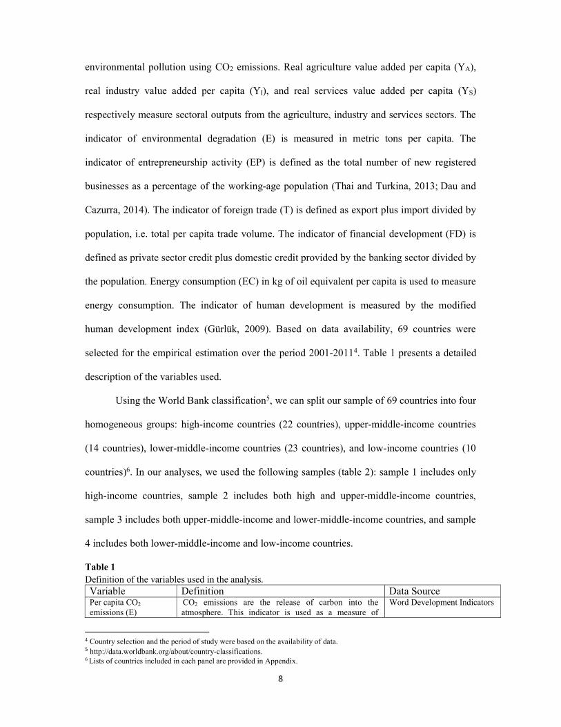
Table 1 Definition of the variables used in the analysis. Variable Definition Data Source Per capita CO2 emissions (E)

CO2 emissions are the release of carbon into the atmosphere. This indicator is used as a measure of

Word Development Indicators

4 Country selection and the period of study were based on the availability of data. 5 http://data.worldbank.org/about/country-classifications. 6 Lists of countries included in each panel are provided in Appendix.

9

environmental degradation. Data is in metric tons per capita.

Entrepreneurship (EP) Measured as the total number of new registered businesses as a percentage of the working-age population.

Global Entrepreneurship Monitor (GEM)

GDP (Y) Measured by per capita US$ (2005). Word Development Indicators Agricultural output (YA) Measured by per capita agricultural value added. Calculated using data from

Word Development Indicators Industrial output (YI) Measured by per capita industry value added. Calculated using data from

World Bank Services output (YS) Measured by per capita services value added. Calculated using data from

Word Development Indicators Foreign trade (T) Defined as export plus import divided by population i.e.

total trade volume per capita. Calculated using data from Word Development Indicators

Financial development (FD)

Defined as private sector credit plus domestic credit provided by banking sector divided by population i.e. financial development per capita.

Calculated using data from World Bank

Energy consumption (EC)

Measured as kg of oil equivalent per capita. Word Bank

Human development (MHDI)

Measured using the modified human development index (MHDI) which measures the average achievements in a country in two basic dimensions of human development (education and life expectancy).

Calculated using data from World Bank

Table2 Samples presentation. Countries Sample 1 Sample 2 Sample 3 Sample 4 High-Income HI HI Upper-Middle-Income UMI UMI Lower-Middle-Income LMI LMI Low-Income LI Total 22 countries 36 countries 37 countries 33 countries

In line with the literature, we formulate the following model:

it 0 1 it 2 it 3 it 4 it 5 it 6 it itE Y EP T FD HDI EC (1)

To test the validity of the EKC hypothesis, we specify and estimate the following

multiple regression equations:

Eit 0 1Yit 2Y2

it 3EPit 4Tit 5FDit 6HDI it 7ECit it (2) 2

it 0 1 it 2 it 3 it 4 it 5 it 6 it 7 it itE EP EP Y T FD HDI EC (3) where i, t, and ɛ are the country, the time period, and the error term respectively. In Eq.2

(EKC), the parameters α1, ….., α7 are the respective CO2 emissions long-run elasticities with

respect to income, squared income, entrepreneurship, trade, financial development, human

10

development and energy consumption. Based on the EKC hypothesis, the expected signs

of Y / E 0 and 2Y / E 0 lead to an inverted U-shaped relationship between emissions

and income growth. In this study, the EKC hypothesis is extended further by replacing real

GDP per capita by sectoral output in order to validate it across sectors. The logic behind this

relationship is that at early stages of economic development, sectoral output induces pollution

( AY / E 0 , IY / E 0 , SY / E 0 ); however, as income rises the incidence of further

environmental damage decreases ( 2AY / E 0 , 2

IY / E 0 , 2SY / E 0 ), due to higher

environmental consciousness and use of modern technology which generates less pollution.

In Eq.3 (MEKC), we replace the square of GDP (Y2) by the square of entrepreneurship

(EP2) in order to examine the quadratic relationship between entrepreneurship and

environmental degradation. The logic underlying this relationship is that at early stages of

economic development, entrepreneurial activity increases real incomes but damages the

environment because at this stage, environmental quality is considered a luxury good.

However, as countries achieve a certain level of economic development, the increased income

from entrepreneurial activity encourages a higher societal demand for a clean environment,

and induces efforts to reduce environmental damage by increasing the number of

environmentally friendly projects and introducing clean production to improve environmental

quality.

2.2. Estimation procedures

In estimating the final versions of Equations (2) and (3) related respectively to the

EKC and MEKC models, we use recently developed panel econometric techniques. They

improve the statistical reliability of our tests by integrating cross-country heterogeneity and

cross-country dependence. For heterogeneous countries, assuming cross-sectional

11

independence across panels could as Banerjee et al. (2004) and others suggest, distort the

results.

To estimate our two models as a panel cointegration model, we consider a three-step

empirical methodology. First, we analyze the cross-sectional dependence and check the

stationarity of the series. Second, we perform a cointegration test to examine the long-run

dynamics of cross-sectional dependence across countries. Third, we estimate the long-run

relationships among the variables using fully modified ordinary least square (FMOLS)

techniques.

2.3.1. Cross-sectional dependence and panel unit root tests

The sample data were examined first using the Pesaran (2004) test for cross-sectional

dependence (CD) to determine the presence of (CD) or cross sectional independence. This is

an important step before applying panel unit root tests. The conventional unit root tests can

provide weak findings due to low power if they are applied to series with CD. Therefore, we

applied the cross-sectionally augmented panel unit root test (CIPS), one of the unit root tests

from the second-generation developed by Pesaran (2007), which assumes that a series is CD.

This unit root test is applied to investigate the order of integration in the series. This is a

prerequisite for panel cointegration models. If the variables considered are I (1), then it can be

concluded that the variables tested are stationary at their first difference, suggesting that this

group of variables may be cointegrated in the long-run. The next subsection provides a

detailed discussion of the panel cointegration test.

2.2.2. Panel cointegration tests

After confirming that the series is stationary by applying the Pesaran (2004) CD test and

Pesaran (2007) CIPS unit root tests to the underlying models, we can perform panel

cointegration analysis. The literature suggests a number of panel cointegration tests e.g. the

Pedroni (1999, 2004) panel cointegration test, and the Kao (1999) panel cointegration test . In

12

our study we want also to check for a long-run equilibrium relationship among the variables,

using the Pedroni (1999, 2004) panel cointegration test. Pedroni suggests seven different

statistics to test for cointegration relationships in heterogeneous panels. These tests are

corrected for bias introduced by potentially endogenous regressors, and are classified into

within dimension and between dimensions statistics. The first sets are described as panel

cointegration statistics, and the second are termed mean panel cointegration statistics.

2.2.3. Panel long-run estimation

After all the variables are cointegrated, the next step is to estimate the associated long-

run cointegration parameters. Fixed effects, random effects and general method of moment

methods can lead to inconsistent and misleading coefficients when applied to cointegrated

panel data. Among the existing panel data cointegration techniques, we use Pedroni (1999)

Fully Modified Ordinary Least Squares (FMOLS) estimator which deals with possible

heteroskedasticity and autocorrelation of the residuals, takes into account the presence of

nuisance parameters, is asymptotically unbiased and, more importantly, deals with potential

endogeneity of regressors. Tables 5 and 6 present the results of the long-run estimations using

the FMOLS method.

4. Results and discussion

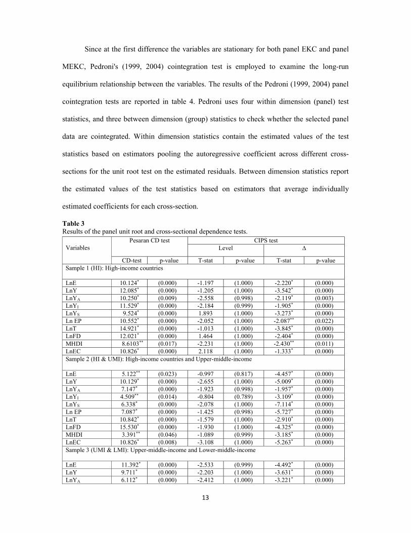
The results in table 3 are for the Pesaran cross-sectional dependence test which is

applied to all variables. The null of cross-sectional independence is rejected for each selected

variable. Formal econometric modeling requires an understating of the integrating properties

of the data. Thus, we apply Pesaran (2007) panel unit root test. Its results are reported in

Table 3 and indicate that all series under consideration are non-stationary at their level form.

However, at first difference level, the all series of variables are integrated. It implies that the

selected series are integrated at I(1) in each panel.

13

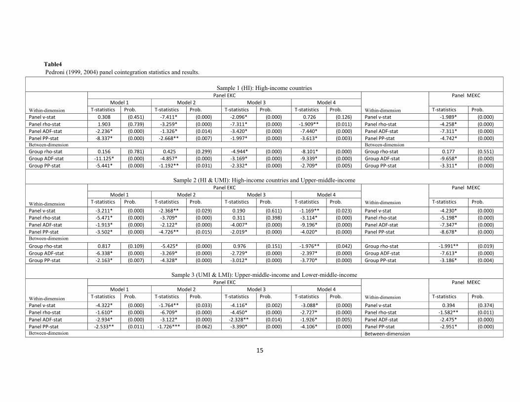
Since at the first difference the variables are stationary for both panel EKC and panel

MEKC, Pedroni's (1999, 2004) cointegration test is employed to examine the long-run

equilibrium relationship between the variables. The results of the Pedroni (1999, 2004) panel

cointegration tests are reported in table 4. Pedroni uses four within dimension (panel) test

statistics, and three between dimension (group) statistics to check whether the selected panel

data are cointegrated. Within dimension statistics contain the estimated values of the test

statistics based on estimators pooling the autoregressive coefficient across different cross-

sections for the unit root test on the estimated residuals. Between dimension statistics report

the estimated values of the test statistics based on estimators that average individually

estimated coefficients for each cross-section.

Table 3 Results of the panel unit root and cross-sectional dependence tests.

Variables

Pesaran CD test CIPS test Level ∆

CD-test p-value T-stat p-value T-stat p-value Sample 1 (HI): High-income countries

LnE 10.124* (0.000) -1.197 (1.000) -2.220* (0.000) LnY 12.085* (0.000) -1.205 (1.000) -3.542* (0.000) LnYA 10.250* (0.009) -2.558 (0.998) -2.119* (0.003) LnYI 11.529* (0.000) -2.184 (0.999) -1.905* (0.000) LnYS 9.524* (0.000) 1.893 (1.000) -3.273* (0.000) Ln EP 10.552* (0.000) -2.052 (1.000) -2.087** (0.022) LnT 14.921* (0.000) -1.013 (1.000) -3.845* (0.000) LnFD 12.021* (0.000) 1.464 (1.000) -2.404* (0.000) MHDI 8.6103** (0.017) -2.231 (1.000) -2.430** (0.011) LnEC 10.826* (0.000) 2.118 (1.000) -1.333* (0.000) Sample 2 (HI & UMI): High-income countries and Upper-middle-income

LnE 5.122** (0.023) -0.997 (0.817) -4.457* (0.000) LnY 10.129* (0.000) -2.655 (1.000) -5.009* (0.000) LnYA 7.147* (0.000) -1.923 (0.998) -1.957* (0.000) LnYI 4.509** (0.014) -0.804 (0.789) -3.109* (0.000) LnYS 6.338* (0.000) -2.078 (1.000) -7.114* (0.000) Ln EP 7.087* (0.000) -1.425 (0.998) -5.727* (0.000) LnT 10.842* (0.000) -1.579 (1.000) -2.910* (0.000) LnFD 15.530* (0.000) -1.930 (1.000) -4.325* (0.000) MHDI 3.391** (0.046) -1.089 (0.999) -3.185* (0.000) LnEC 10.826* (0.008) -3.108 (1.000) -5.263* (0.000) Sample 3 (UMI & LMI): Upper-middle-income and Lower-middle-income

LnE 11.392* (0.000) -2.533 (0.999) -4.492* (0.000) LnY 9.711* (0.000) -2.203 (1.000) -3.631* (0.000) LnYA 6.112* (0.000) -2.412 (1.000) -3.221* (0.000)

14

LnYI 8.298* (0.000) -1.883 (0.958) -2.705* (0.000) LnYS 4.651* (0.002) -2.118 (1.000) -2.150* (0.000) Ln EP 4.475* (0.003) -1.699 (1.000) -2.625* (0.000) LnT 10.179* (0.000) -2.560 (1.000) -3.002* (0.000) LnFD 12.615* (0.000) -1.704 (1.000) -3.529* (0.000) MHDI 6.297* (0.000) -2.593 (1.000) -2.057* (0.000) LnEC 2.574* (0.000) -1.856 (0.889) -2.119* (0.000) Sample 4 (LMI & LI): Lower-middle-income and Low-income

LnE 10.390* (0.000) -2.233 (0.765) -3.397* (0.000) LnY 6.711* (0.000) -1.703 (1.000) -2.930* (0.000) LnYA 6.252* (0.000) -1.712 (1.000) -2.920* (0.000) LnYI 9.348* (0.000) -2.083 (0.958) -3.005* (0.000) LnYS 5.601* (0.000) -2.108 (0.941) -3.050* (0.000) Ln EP 7.475* (0.000) -1.719 (1.000) -2.921* (0.000) LnT 7.179* (0.000) -1.720 (1.000) -2.902* (0.000) LnFD 11.61* (0.000) -1.754 (1.000) -3.322* (0.000) MHDI 7.181* (0.000) -2.192 (0.880) 3.365 * (0.000) LnEC 6.895* (0.000) -2.179 (0.900) -2.877 * (0.000)

Notes: All panel unit root tests were performed with restricted intercept and trend for all the variables. * and ** are statistical significance at the 1% and 5% levels, respectively.

The results of the within dimension tests and the between dimension tests provide

strong evidence that the null hypothesis of no cointegration in each panel should be rejected.

Having confirmed the cointegration between these variables, in the next step we estimate the

long-run coefficients. The test-statistics for all seven tests show that the null hypothesis of no

cointegration can be rejected. Therefore, in our sample period, all the variables we consider

have long-run associations. This leads to the conclusion that the variables considered are

cointegrated for the four samples, and share a two long run equilibrium relationship with all

the variables in eqs. (2) and (3). After confirming the cointegration among variables is

confirmed, the long-run coefficients are estimated.

15

Table4 Pedroni (1999, 2004) panel cointegration statistics and results.

Sample 1 (HI): High-income countries

Within-dimension

Panel EKC Within-dimension

Panel MEKC Model 1 Model 2 Model 3 Model 4

T-statistics Prob. T-statistics Prob. T-statistics Prob. T-statistics Prob. T-statistics Prob. Panel v-stat 0.308 (0.451) -7.411* (0.000) -2.096* (0.000) 0.726 (0.126) Panel v-stat -1.989* (0.000) Panel rho-stat 1.903 (0.739) -3.259* (0.000) -7.311* (0.000) -1.909** (0.011) Panel rho-stat -4.258* (0.000) Panel ADF-stat -2.236* (0.000) -1.326* (0.014) -3.420* (0.000) -7.440* (0.000) Panel ADF-stat -7.311* (0.000) Panel PP-stat -8.337* (0.000) -2.668** (0.007) -1.997* (0.000) -3.613* (0.003) Panel PP-stat -4.742* (0.000) Between-dimension Between-dimension Group rho-stat 0.156 (0.781) 0.425 (0.299) -4.944* (0.000) -8.101* (0.000) Group rho-stat 0.177 (0.551) Group ADF-stat -11.125* (0.000) -4.857* (0.000) -3.169* (0.000) -9.339* (0.000) Group ADF-stat -9.658* (0.000) Group PP-stat -5.441* (0.000) -1.192** (0.031) -2.332* (0.000) -2.709* (0.005) Group PP-stat -3.311* (0.000)

Sample 2 (HI & UMI): High-income countries and Upper-middle-income Within-dimension

Panel EKC Within-dimension

Panel MEKC Model 1 Model 2 Model 3 Model 4

T-statistics Prob. T-statistics Prob. T-statistics Prob. T-statistics Prob. T-statistics Prob. Panel v-stat -3.211* (0.000) -2.368** (0.029) 0.190 (0.611) -1.169** (0.023) Panel v-stat -4.230* (0.000) Panel rho-stat -5.471* (0.000) -3.709* (0.000) 0.311 (0.398) -3.114* (0.000) Panel rho-stat -5.198* (0.000) Panel ADF-stat -1.913* (0.000) -2.122* (0.000) -4.007* (0.000) -9.196* (0.000) Panel ADF-stat -7.347* (0.000) Panel PP-stat -3.502* (0.000) -4.726** (0.015) -2.019* (0.000) -4.020* (0.000) Panel PP-stat -8.678* (0.000) Between-dimension Group rho-stat 0.817 (0.109) -5.425* (0.000) 0.976 (0.151) -1.976** (0.042) Group rho-stat -1.991** (0.019) Group ADF-stat -6.338* (0.000) -3.269* (0.000) -2.729* (0.000) -2.397* (0.000) Group ADF-stat -7.613* (0.000) Group PP-stat -2.163* (0.007) -4.328* (0.000) -3.012* (0.000) -3.770* (0.000) Group PP-stat -3.186* (0.004)

Sample 3 (UMI & LMI): Upper-middle-income and Lower-middle-income Within-dimension

Panel EKC Within-dimension

Panel MEKC Model 1 Model 2 Model 3 Model 4

T-statistics Prob. T-statistics Prob. T-statistics Prob. T-statistics Prob. T-statistics Prob. Panel v-stat -4.322* (0.000) -1.764** (0.033) -4.116* (0.002) -3.088* (0.000) Panel v-stat 0.394 (0.374) Panel rho-stat -1.610* (0.000) -6.709* (0.000) -4.450* (0.000) -2.727* (0.000) Panel rho-stat -1.582** (0.011) Panel ADF-stat -2.934* (0.000) -3.122* (0.000) -2.328** (0.014) -1.926* (0.005) Panel ADF-stat -2.475* (0.000) Panel PP-stat -2.533** (0.011) -1.726*** (0.062) -3.390* (0.000) -4.106* (0.000) Panel PP-stat -2.951* (0.000) Between-dimension Between-dimension

16

Group rho-stat -3.261* (0.000) -4.425* (0.000) -2.558* (0.005) -2.976* (0.000) Group rho-stat 0.912 (0.196) Group ADF-stat -1.899** (0.019) -2.269* (0.000) -4.364* (0.000) -3.552* (0.000) Group ADF-stat -4.339* (0.000) Group PP-stat -3.036* (0.000) -2.328* (0.000) -3.671* (0.000) -2.268* (0.004) Group PP-stat -5.016* (0.000)

Sample 4 (LMI & LI): Lower-middle-income and Low-income Within-dimension

Panel EKC

Within-dimension

Panel MEKC Model 1 Model 2 Model 3 Model 4

T-statistics Prob. T-statistics Prob. T-statistics Prob. T-statistics Prob. T-statistics Prob. Panel v-stat -4.009* (0.000) -4.083* (0.000) 0.245 (0.489) -5.001* (0.000) Panel v-stat -0.912*** (0.053) Panel rho-stat -1.999* (0.000) -2.197** (0.027) -2.171** (0.017) -2.325* (0.000) Panel rho-stat -2.193** (0.011) Panel ADF-stat -3.416* (0.000) -4.379* (0.000) -3.130* (0.000) -5.291* (0.000) Panel ADF-stat -3.148* (0.000) Panel PP-stat -2.313* (0.000) -1.313*** (0.052) -1.572** (0.020) -3.123* (0.000) Panel PP-stat -2.081* (0.000) Between-dimension Between-dimension Group rho-stat -3.880* (0.000) -6.320* (0.000) 0.379 (0.326) -4.267* (0.000) Group rho-stat -1.408* (0.000) Group ADF-stat -2.239* (0.000) -1.829* (0.007) -4.279* (0.000) -2.627* (0.000) Group ADF-stat -3.322* (0.000) Group PP-stat -2.674* (0.000) -2.499* (0.000) -4.189* (0.000) -2.394* (0.000) Group PP-stat -2.910* (0.000)

The null hypothesis of Pedroni's test examines the absence of cointegration. Lag selection (automatic) is based on SIC with a max lag of 5. *, ** and *** represent the statistical significance at the 1%, 5% and 10% levels, respectively.

17

Tables 5 and 6 present the results of the respective panel FMOLS estimates for EKC

and MEKC. All the variables except the MHDI variable are expressed in natural logarithms.

The estimated coefficients of the long-run cointegration relationship can be interpreted as

long-run elasticities. Tables 5 and 6 show that environmental degradation is a positive

function of output growth, financial development, and energy consumption. This finding is in

line with most previous studies (see Omri, 2013; Apergis and Payne, 2014). It can generally

be observed that the rate of environmental degradation due to GDP or sectoral outputs is

much higher in case of low-income economies with inadequate, unsophisticated, and

primitive production technologies, poor environmental regulation, etc. However, a first look

at the results in tables 5 and 6 reveal an interesting pattern for the relationship between output

growth and environmental degradation. While GDP has a positive and statistically significant

impact on environmental degradation across the different four samples considered, long-run

elasticity of GDP is much higher in sample 2 (upper-middle-income and high-income

countries -0.199) and sample 1 (high-income countries -0.158), compared to sample 4 (lower-

middle-income and low-income countries -0.087). What is the reason for these unexpected

but robust results? Can it be argued that compared to high-income and upper-middle-income

countries, those countries with the lowest incomes have achieved far more environmentally

efficient economic growth? These questions require more research. The general economic

rationale indicates that higher income countries generally rely more on services and industry

sectors to enhance their economic growth, these sectors use more energy either directly or

indirectly, which results in more emissions. So, since high-income countries are responsible

for most of the world's environmental pollution, the level of their environmental conservation

efforts is evidently insufficient. Given their prosperity and economic size, they should channel

more resources and logistics to reduce CO2 emissions arising from energy use, most of which

comes from fossil fuels. It is important for these countries to use cleaner and more efficient

18

fossil fuel sources such as natural gas and higher-grade coal. It is important for them to

increase use of renewable energy sources such as hydro, solar, geothermal, and wind. These

countries should devote serious effort to technology advances to achieve a balance between

economic growth and environmental conservation which is a public good. Such efforts would

control and reduce environmental pollution without harming economic growth and

development. Moreover, levels of energy use differ between those countries with the highest

income and those with lowest income. The high-income countries consume the lion's share of

the world's energy resources. Moreover, levels of energy use differ between those countries

with the highest income and those with lowest income. The high-income countries consume

the lion's share of the world's energy resources. In addition to the impact of output, we find

that energy consumption has a positive and significant impact on environmental degradation

in all four samples, indicating that environmental degradation is elastic with respect to energy

consumption, and a 1% increase in energy consumption increases environmental degradation

within the range 0.194% for the high-income (HI) sample and 0.098% for the lower-middle-

income and low-income (LMI & LI) samples. This finding is in line with Omri and Kahouli

(2014). Moreover, financial development exhibits a generally positive impact on

environmental degradation in all but the high-income sample; however, this is statistically

significant only for middle-income (UMI & LMI) samples. Its impact is negative and

significant for the high-income sample (-0.027), indicating that, in high income countries,

financial development can lead to technological innovation which contributes significantly to

reducing environmental damage (King and Levine, 1993). Also, technological innovation

promotes environmentally friendly production by easing the access to financial resources

(Tamazian et al., 2009), and helping investors to use new and advanced technology for more

environmentally friendly production (Shahbaz et al., 2013). Human development has a

negative and statistically significant impact on environmental degradation for all except the

19

low-income countries. This result is in line with Costantini and Monni (2008). Finally, trade

openness has a negative impact on environmental degradation in most of the countries

considered; however, it is statistically significant only in the case of high-income, lower-

middle-income and low-income countries. In addition, the impact is higher in the case of the

lower-middle-income and low-income samples compared to the high-income sample. This is

because foreign trade requires the trading countries, particularly low-income countries, to

undertake rigorous and standardized environmental actions in their manufacturing processes

in order to export to high-income countries.

Table 5 Panel FMOLS Long-run Elasticity Estimates for EKC.

Independent variables

Dependent variable : Environmental degradation (E) Model 1 Model 2 Model 3 Model 4

Coef. Prob. Coef. Prob. Coef. Prob. Coef. Prob.

Sample 1 (HI): High-income countries LnY 0.158* (0.003) - - - - - - LnY2 -0.077 (0.120) - - - - - - Ln YA - - 0.125** (0.019) - - - - LnYA2 - - -0.082 (0.134) - - - - Ln YI - - - - 0.147*** (0.067) - - LnYI2 - - - - -0.054 (0.198) - - Ln YS - - - - - - 0.164* (0.000) LnYS2 - - - - - - -0.066 (0.152) LnEP 0.065* (0.007) 0.049** (0.010) 0.075** (0.019) 0.061*** (0.056) LnT -0.094** (0.035) -0.079*** (0.088) -0.103** (0.024) -0.098*** (0.095) LnFD -0.027** (0.035) 0.116* (0.005) 0.131* (0.003) 0.114** (0.022) MHDI -0.127*** (0.058) -0.075*** (0.091) -0.121*** (0.089) -0.109** (0.037) LnEC 0.194* (0.004) 0.141** (0.042) 0.191* (0.000) 0.199** (0.014) Constant 0.230** (0.012) 0.184* (0.000) 0.255*** (0.056) 0.179* (0.000)

Sample 2 (HI & UMI): High-income countries and Upper-middle-income LnY 0.199** (0.015) - - - - - - LnY2 -0.111** (0.017) - - - - - - Ln YA - - 0.102*** (0.092) - - - - LnYA2 - - -0.100**v (0.077) - - - - Ln YI - - - - 0.112** (0.014) - - LnYI2 - - - - 0.054 (0.206) - - Ln YS - - - - - - 0.131 (0.104) LnYS2 - - - - - - -0.066 (0.152) LnEP 0.097* (0.000) 0.103* (0.000) 0.077*** (0.094) 0.111** (0.018) LnT -0.044 (0.105) -0.102 (0.152) 0.112 (0.103) -0.046 (0.190) LnFD 0.099 (0.114) 0.102** (0.012) 0.092*** (0.061) 0.097* (0.000) MHDI -0.097** (0.034) -0.056** (0.011) -0.105* (0.004) -0.098*** (0.074) LnEC 0.151* (0.000) 0.110*** (0.071) 0.201* (0.000) 0.184*** (0.052) Constant 0.196* (0.001) 0.225* (0.008) 0.172*** (0.081) 0.189*** (0.066)

Sample 3 (UMI & LMI): Upper-middle-income and Lower-middle-income LnY .0141*** (0.049) - - - - - - LnY2 -0.099** (0.012) - - - - - - Ln YA - - 0.071 (0.130) LnYA2 - - -0.064*** (0.094) - - - -

20

Ln YI - - - - 0.104** (0.018) LnYI2 - - - - -0.095* (0.000) - - Ln YS - - - - - - -0.097** (0.013) LnYS2 - - - - - - -0.023 (0.164) LnEP 0.129* (0.000) 0.135** (0.027) 0.128* (0.000) 0.134** (0.040) LnT -0.109 (0.114) -0.091 (0.124) 0.054 (0.178) 0.101 (0.113) LnFD 0.106** (0.033) 0.077** (0.033) -0.081 (0.124) 0.089** (0.040) MHDI -0.084*** (0.056) 0.033 (0.172) -0.077** (0.033) -0.068 (0.109) LnEC 0.123** (0.010) 0.081*** (0.058) 0.114** (0.011) 0.097*** (0.075) Constant 0.219** (0.011) 0.099** (0.017) 0.191*** (0.067) 0.202* (0.000)

Sample 4 (LMI & LI): Lower-middle-income and Low-income LnY 0.087** (0.024) - - - - - - LnY2 -0.079** (0.043) - - - - - - Ln YA - - 0.096** (0.040) - - - - LnYA2 - - -0.081*** (0.085) - - - - Ln YI - - - - 0.088*** (0.059) LnYI2 - - - - -0.084** (0.014) Ln YS - - - - - - -0.117*** (0.087) LnYS2 - - - - - - 0.094 (0.124) LnEP 0.225** (0.020) 0.201* (0.003) 0.294** (0.016) 0.188* (0.000) LnT -0.152* (0.000) -0.111** (0.022) -0.148* (0.001) -0.087*** (0.072) LnFD 0.132 (0.108) 0.054** (0.011) 0.046*** (0.082) 0.070** (0.010) MHDI -0.031 (0.215) -0.072 (0.121) 0.069 (0.192) -0.038 (0.236) LnEC 0.098** (0.029) 0.056 (0.198) 0.098 (0.122) 0.043 (0.215) Constant 0.197* (0.000) 0.312* (0.000) 0.124** (0.036) 0.176* (0.003)

P-values are reported in parentheses. *, ** and *** represent the statistical significance at the 1%, 5% and 10% levels, respectively. Table 6 Panel FMOLS Long-run Elasticity Estimates for MEKC.

Independent variables

Dependent variable : Environmental degradation (E) Sample 1: HI Sample 2: HI & UMI Sample 3: UMI &LMI Sample 4: LMI & LI

Coef. Prob. Coef. Prob. Coef. Prob. Coef. Prob.

LnEP 0.084*** (0.057) 0.080** (0.041) 0.114** (0.039) 0.136*** (0.073) LnEP2 -0.066** (0.033) -0.051 (0.108) -0.011 (0.273) 0.038 (0.136) LnY 0.191** 0.025) 0.146* (0.008) 0.111 (0.138) 0.124** (0.029) LnT -0098* (0.000) -0.073 (0.124) 0.110 (0.104) -0.122** (0.018) LnFD 0.117** (0.022) 0.124*** (0.060) 0.084 (0.128) 0.101 (0.146) MHDI -0.088*** (0.089) -0.067** (0.046) -0.091 (0.162) -0.078 (0.124) LnEC 0.231* (0.000) 0.219** (0.014) 0.175* (0.005) 0.170*** (0.086) Constant 0.265* (0.002) 0.456* (0.000) 0.184*** (0.063) 0.171** (0.020)

P-values are reported in parentheses. *, ** and *** represent the statistical significance at the 1%, 5% and 10% levels, respectively.

After generalizing the result of the effect of per capita GDP on CO2 emissions across

samples, now we answer if the increase of economic growth constitutes a motivation to strive.

The results of model 1 (Table 5) show the existence of EKC with a negative and statistically

significant coefficient of Y2 and a positive and statistically significant coefficient of Y across

all but the high-income sample and sectors. The existence of an EKC is not conclusively

supported for the high-income (HI) sample because the coefficient of Y (or YA, YI, YS) is

positive and significant but the coefficient of Y2 (or Y2A, Y2I, Y2S) is negative and

21

insignificant. This is a robust result which contradicts many empirical findings. Therefore, we

cannot fully confirm the first hypothesis.

Finally, we focus on an important gap in the research i.e. understanding how

entrepreneurship and different sectoral outputs contribute to environmental improvement in

different ways based on countries' stages of economic development or income levels. Table 5

and 6 show that the impact of entrepreneurial activity on environmental degradation is

positive and statistically significant for all the samples considered. However, we found that

this impact is relatively lower in the case of the high-income sample compared to the other

samples. Previous efforts to address this issue focus only on how and why existing firms

become greener (Cohen and Winn, 2007; Haal et al., 2010; York and Venkataraman, 2010).

Haal et al. (2010) suggest that entrepreneurship may be the solution to many social and

environmental problems, and could provide the way to a more sustainable future. However,

when we include EP2 in the estimated model, this parameter becomes negative and

statistically significant only for the high-income sample, indicating that in the early stages of

economic development environmental degradation increases with entrepreneurial activities

but that after a certain level of entrepreneurship, environmental degradation starts to improve.

This result confirms our second hypothesis. Despite the existence of an EKC between

entrepreneurship and environmental degradation for the high-income sample, since the

coefficient of EP is higher than the coefficient of EP2, an increase in entrepreneurial activities

will have a smaller effect on reducing long run environmental degradation. This means that

current efforts to reduce environmental pollution will be ineffective. Cohen and Winn (2007:

p.30) suggest the need for entrepreneurial actions in order to resolve our environmental

problems, and suggest also that “the real gains will only be made by harnessing the innovative

potential of entrepreneurs who will develop the innovative business solutions to deal with the

environmental challenges”.

22

The results for the contribution of sectoral outputs to the environmental degradation

(table 5) provide some robust conclusions. Models 1-3 show that the industrial sector has a

positive and statistically significant impact on environmental degradation in all four country

samples, indicating that environmental degradation is elastic with respect to industry output,

and that a 1% increase in industry output increases environmental degradation within the

range 0.147% for the high-income sample and 0.088% for the lower-middle-income and low-

income sample. So, countries with higher levels of income generally rely on their industrial

sector to enhance economic growth. Clearly, this sector uses more energy - either directly or

indirectly - which engenders more environmental damage. In addition, the impact of service

sector on the CO2 emissions across samples generally confirms that a move from an industrial

economy to a services economy is not favorable to economic transformation in high-income

countries. However, it does reduce environmental degradation in the upper-middle-income

and lower-middle-income (samples 3) countries, and the lower-middle-income and low-

income (Sample 4) countries. The service sector contributes positively to environmental

degradation in the case of the high-income sample (0.164) but has a statistically negative

impact for the other samples. Finally, the impact of agricultural output is positive and

statistically significant in all the samples except sample 3 (middle-income countries). It shows

that a 1% increase in agricultural output increases environmental degradation by 0.096 for the

lower-middle-income and low-income countries, by 0.102 for the high-income and upper-

middle-income countries, and by 0.125 for the high-income countries. Thus, agricultural

output makes the smallest contribution to environmental degradation in low income countries

which depend heavily on primitive agricultural technologies and logistics which reduce

environmental emissions. The above results allow us to conclude that the services sector in

high-income countries makes a much higher contribution to environmental degradation

23

compared to the agriculture and industry sectors. In this context, Alcanatra and Padilla (2008),

O’Mahony et al. (2012) show that the services sector is responsible for the lion's share of CO2

emissions compared to other economic sectors, and that the transport sector which is one of

the major subsectors of services accounts for most of these emissions. Due to the strong

impact of services on other economic sectors, the direct and indirect impact of services output

on environmental pollution is rising steadily. Since the services sector in high-income

countries is the highest contributor to environmental pollution compared to other sectors,

policies to reduce their emissions require a better understanding of the services sector which

takes account of wholesale and retail trade, hotels and restaurants, transportation, tourism ,

and other subsectors. In this context, O’Mahony et al. (2012) show that services subsectors

contribute a great deal to environmental pollution compared to other sectors, and that

increases in the transport sector are resulted in significantly increased environmental damage.

However, services tend to be less of a focus in the design of policies aimed at reducing

environmental pollution.

5. Conclusions and implications

This paper contributes to the existing literature on environmental sustainability by

explaining how entrepreneurship and different sectoral outputs can help to improve

environmental quality for 69 countries split across four homogeneous income-based panels:

high-income, upper-middle-income, lower-middle-income, and low-income economies.

It provides several important results. First, the CO2 emissions due to the output growth

is larger for high-income countries which generally rely on the service and industry sectors

for enhanced growth and development, and these sectors use more energy which results in the

larger CO2 emissions. Second, the services sector is the biggest contributor to environmental

pollution compared to other sectors in high-income countries. For the middle-income and

24

lower-middle-income and low-income countries its contribution is negative; indicating that

the move from an industrial and agricultural economy to services economy is beneficial for

these countries. Third, there is an EKC relationship between output growth and environmental

degradation across all panels and sectors except the high-income group. Fourth, the

contribution of entrepreneurship to environmental degradation is lower in the case of high-

income countries compared to the other country samples. Fifth, entrepreneurial activity

contributes to the environmental improvement only for the high-income countries. Sixth,

trade openness and human development generally have reduced the world’s emissions.

Our findings helped us to give some serious policy implications in order to improve

the environmental quality across the world. First, since high-income countries are responsible

for most of the world's environmental pollution, the level of their environmental conservation

efforts is evidently insufficient. Given their prosperity and economic size, they should channel

more resources and logistics to reduce CO2 emissions arising from energy use, most of which

comes from fossil fuels. It is important for these countries to use cleaner and more efficient

fossil fuel sources such as natural gas and higher-grade coal. It is important for them to

increase use of renewable energy sources such as hydro, solar, geothermal, and wind. These

countries should devote serious effort to technology advances to achieve a balance between

economic growth and environmental conservation which is a public good. Such efforts would

control and reduce environmental pollution without harming economic growth and

development. Second, despite the existence of an EKC between entrepreneurship and

environmental degradation for the high-income sample, since the coefficient of EP is higher

than the coefficient of EP2, an increase in entrepreneurial activities will have a smaller effect

on reducing long run environmental degradation. This means that current efforts to reduce

environmental pollution will be ineffective. In this context, Cohen and Winn (2007: p.30)

suggest the need for entrepreneurial actions in order to resolve our environmental problems,

25

and suggest also that “the real gains will only be made by harnessing the innovative potential

of entrepreneurs who will develop the innovative business solutions to deal with the

environmental challenges”. To encourage these businesses, large and small, to comply with

the different principles of sustainable development, two means are regularly identified:

coercive means and more determined (voluntary) means. The first ones are employed by

governments through laws and regulations, while the latter relate to voluntary commitments

from companies themselves through corporate social responsability (CSR).

Appendix Table A1 List of countries included

High-income Upper-middle-income Lower-middle-income Low-income - Austria - Australia - Belgium - Finland - France - Hungary - Ireland - Italy - Japan - Korea Republic - Luxembourg - Netherlands - New Zealand - Norway - Poland - Portugal - Singapore - Spain - Sweden - Switzerland - United Kingdom - United States

- Algeria - Angola - Brazil - Bulgaria - Chile - China - Colombia - Costa Rica - Jordan - Mexico - Romania - South Africa - Thailand - Turkey

- Albania - Argentina - Cameroon - Cape Verde - Cote d’Ivoire - Egypt - El Salvador - Ghana - Honduras - India - Indonesia - Mongolia - Nicaragua - Pakistan - Guinea - Paraguay - Philippines - Senegal - Syrian Arab Republic - Sri Lanka - Sudan - Vietnam - Zambia

- Bangladesh - Benin - Burkina Faso - Bolivia - Ethiopia - Kenya - Liberia - Mozambique - Uganda - Zimbabwe

References

1. Acs, Z.J., Audretsch, D.B., Feldman, M.P., 1994. R&D spillovers and recipient firm size. Review of Economics and Statistics 100, 336–367.

2. Alcanatra, V., Padilla, E., 2008. Input–output subsystems and pollution: application to the service in Spain. Ecological Economics 68, 905–14.

26

3. Al-mulali, U., Saboori, B., Ozturk, I., 2015. Investigating the environmental Kuznets curve hypothesis

in Vietnam. Energy Policy 76, 123–131.

4. Ang, J.B., 2007. CO2 emissions, energy consumption, and output in France. Energy Policy 35, 4772–4778.

5. Apergis, N., Payne, J.E., 2010. Energy consumption and growth in South America: Evidence from a panel error correction model. Energy Economics 32, 1421–1426.

6. Apergis, N., Payne, J.E., 2014. Renewable energy, output, CO2 emissions, and fossil fuel prices in Central America: Evidence from a nonlinear panel smooth transition vector error correction model. Energy Economics 42, 226–232.

7. Azomahou, T., Laisney, F. and P. Nguyen Van, P. 2006. Economic development and CO2 emissions: A

nonparametric panel approach, Journal of Public Economics 90, 1347–1363.

8. Baltagi, B.H., 2009. A Companion to Econometric Analysis of Panel Data. Chichester, UK: Wiley.

9. Bai, J., Ng, S., 2004. A panic attack on unit roots and cointegration. Econometrica 72, 1127-1177.

10. Breitung, J., Pesaran, M.H., 2008. Unit roots and cointegration in panels. In: Matyas, L., Sevestre, P. (Eds.), The Econometrics of Panel Data, third ed. Springer-Verlag.

11. Carson, R., Lear, L., Wilson, E.O., 2003. Silent Spring, 40th ed. Houghton Mifflin Company, Boston.

12. Cialini.C., 2007, Economic growth and environmental quality An econometric and a decomposition analysis, Management of Environmental Quality: An International Journal 18, 568-577.

13. Cho, C.H., Chu, Y.P., Yang, H.Y., 2014. An environment Kuznets curve for GHG emissions: a panel cointegration analysis. Energy Sources Part B: Economics, Planning, and Policy 9, 120–129.

14. Chudik, A., M. H. Pesaran, and E. Tosetti., 2011. Weak and strong cross section dependence and estimation of large panels. The Econometrics Jounal 14, 45-90.

27

15. Cohen, B., Winn, M.I., 2007. Market imperfections, opportunity and sustainable entrepreneurship. Journal of Business Venturing 22, 29 – 49.

16. Costantini, V., Monni, S., 2008. Environment, human development, and economic development. Ecological Economics 64, 867–880.

17. Dau, L.A., Cazurra, A.C., 2014. To formalize or not to formalize: Entrepreneurship and pro-market institutions. Journal of Business Venturing 29, 668–686.

18. De Hoyos, R.E., Sarafidis, V., 2006. Testing for cross–sectional dependence in panel–data models. The Stata Journal 6, 482–496.

19. Driscoll, J. C., Kraay, A. C., 1998. Consistent Covariance Matrix Estimation with Spatially Dependent Panel Data. Review of Economics and Statistics 80, 549–560.

20. Du, L., Wei, Chu, Cai, S., 2012. Economic development and carbon dioxide emissions in China: provincial panel data analysis. China Economic Review 23, 371–384.

21. Engle, R.F., Granger, C.W.J., 1987. Co-integration and error correction: representation, estimation, and testing. Econometrica 55, 251–276.

22. Farhani, S., Mrizak, S.,Chaibi, A.,Rault, C., 2014. The environmental Kuznets Curve and Sustainability: A panel data analysis. Energy Policy 17, 189–198.

23. Flannery, T., 2005. The Weather Makers. Grove Press, New York, NY.

24. Friedl, B., Getzner, M., 2003. Determinants of CO2 emissions in a small open economy. Ecological Economics 45, 133–148.

28

25. Grossman, G.M., Krueger, A.B., 1991. Environmental Impact of a North American Free Trade Agreement. NBER Working Paper 3914. Cambridge, MA: National Bureau of Economic Research.

26. Grossman, G. M., Krueger A. B., 1993. Environmental Impacts of A North American Free Trade Agreement." In Barber P. (ed.), The US-Mexico Free Trade Agreement. MIT Press, Cambridge, MA.

27. Gürlük, S., 2009. Economic growth, industrial pollution and human development in the Mediterranean region. Ecological Economics 68, 2327–2335.

28. Habbershon, T., Nordqvist, M., Zellweger, T. M., 2010. Transgenerational Entrepreneurship. In M.

Nordqvist & T. Zellweger (Eds.), Transgenerational Entrepreneurship: Exploring Growth and Performance in Family Firms across Generations (pp. 1-38). Cheltenham: Edward Elgar.

29. Halicioglu, F., 2009. An econometric study of CO2 emissions, energy consumption, income and foreign trade in Turkey. Energy Policy 37, 1156–1164.

30. Hall, J.K., Daneke, G.A.., Lenox M.J., 2010. Sustainable Development and Entrepreneurship: Past

Contributions and Future Directions. Journal of Business Venturing 25, 439–448.

31. Han, C., Lee, H., 2013. Dependence of economic growth on CO2 emissions. Journal of economic development 38, 47–57.

32. He, J., Richard, P., 2010. Environmental Kuznets curve for CO2 in Canada. Ecological Economics 69, 1083–1093.

33. Im, K.S., Pesaran, M.H., Shin, Y., 2003. Testing for unit roots in heterogeneous panels. Journal of Econometrics 115, 53–74.

34. Iyigun, N. O., Keskin, M., 2015. Is franchising an efficient tool for entrepreneurship in the knowledge? 15th EBES conference proceedings book, pp. 892–899.

29

35. Jun, Y., Zhong-Kui, Y., Peng-Fei, S., 2011. Income Distribution, Human Capital and Environmental Quality: Empirical Study in China. Energy Procedia 5, 1689–1696.

36. Kao, C., 1999. Spurious regression and residual-based tests for cointegration in panel data. Journal of

Econometrics 90, 1–44.

37. Kaika, D., Zervas, E., 2013a. The Environmental Kuznets Curve (EKC) theory—Part A: Concept, causes and the CO2 emissions case. Energy Policy 62, 1392–402.

38. Kaika, D., Zervas, E., 2013b. The environmental Kuznets curve (EKC) theory. Part B: Critical issues. Energy Policy 62, 1403–11.

39. King, R.G., Levine, R., 1993. Finance and growth: Schumpeter might be right. The Quarterly Journal of Economics 108, 717–737.

40. Lau, L.S., Choong, C.K., Eng, Y.K., 2014. Carbon dioxide emission, institutional quality, and economic growth: Empirical evidence in Malaysia. Renewable Energy 68, 276–281.

41. Levin, A., Lin, C.F., Chu, C.S., 2002. Unit root tests in panel data: Asymptotic and finite sample

properties. Journal of Econometrics 108, 1–24.

42. Li, K., Lin, B., 2015. Metafroniter energy efficiency with CO2 emissions and its convergence analysis

for China. Energy Economics 48, 230–241.

43. Maddala, G.S., Wu, S., 1999. A comparative study of unit root tests with panel data and a new simple test. Oxford Bulletin of Economics and Statistics 631-652.

30

44. Ozturk, I., Acaravci, A., 2013. The long-run and causal analysis of energy, growth, openness and financial development on carbon emissions in Turkey. Energy Economics 36, 262–267.

45. Ozturk, I., Acaravci, A., 2010. CO2 emissions, energy consumption, and economic growth in Turkey.

Renewable and Sustainable Energy Reviews 14, 3220–3225.

46. Omri, A., 2013. CO2 emissions, energy consumption and economic growth nexus in MENA countries:

evidence from simultaneous equations models. Energy Economics 40, 657–664.

47. Omri, A., Daly, S., Chaibi, A., Rault, C. 2015. Financial development, environmental quality, trade and

economic growth: What causes what in MENA countries. Energy Economics 48, 242-252.

48. Omri, A., Kahouli, B., 2014. The nexus among foreign investment, domestic capital and economic

growth: Empirical evidence from the MENA region. Research in Economics 68, 257–263.

49. O’Mahony, T., Zhou, P., Sweeney, J., 2012. The driving forces of energy-related CO2 emissions in Ireland: A multi-sectoral decomposition from 1990 to 2007. Energy Policy 44, 256–267.

50. Pedroni, P., 1999. Critical values for cointegration tests in heterogeneous panels with multiple regressors. Oxford Bulletin of Economics and Statistics 61, 653–670.

51. Pedroni, P., 2004. Panel cointegration: asymptotic and finite sample properties of pooled time series

tests with an application to the PPP hypothesis. Econometric Theory 20, 597–625.

52. Phillips, P.C.B., Moon, H.R., 1999. Linear regression limit theory for non stationary panel data. Econometrica 67, 1057–1112.

53. Pesaran, M., 2007. A simple panel unit root test in the presence of cross-section dependence. Journal of

Applied Econometrics 22, 265–312.

31

54. Pedroni, P., 2001. Purchasing power parity tests in cointegrated panels. The Review of Economics and Statistics 83, 727–731.

55. Riti, J.S., Dankumo, A.M., Gubak, H.D., 2015. Entrepreneurship and Environmental Sustainability: Evidence from Nigeria. Journal of Economics and Sustainable Development 6, 2222–2855.

56. Shahbaz, M., Lean, H.H., Shabbir, M.S., 2012. Environmental Kuznets curve hypothesis in Pakistan: cointegration and Granger causality. Renewable and Sustainable Energy Reviews 16, 2947–2953.

57. Sheperd, D. A. & Patzel, H. (2011). The new field of sustainable entrepreneurship: Studying entrepreneurial action linking “what is to be sustained” with “what is to be developed.” Entrepreneurship Theory and Practice 35, 137– 226.

58. Sahin, T.K., Asunakutlu, T., 2014. Entrepreneurship in a Cultural Context: A Research on Turks in

Bulgaria. Procedia-Social and Behavioral Sciences 150, 851–861.

59. Sheperd, D. A., Patzel, H., 2011. The new field of sustainable entrepreneurship: Studying

entrepreneurial action linking “what is to be sustained” with “what is to be developed. Entrepreneurship Theory and Practice 35, 137–226.

60. Shahbaz, M., Mutascu, M., Azim, P., 2013. Environmental Kuznets curve in Romania and the role of energy consumption. Renewable and Sustainable Energy Reviews 18,165–173.

61. Tamazian, A., Chousa, J.P., Vadlamannati, K.C., 2009. Does higher economic and financial development lead to environmental degradation: Evidence from BRIC countries. Energy Policy 37, 246–253.

32

62. Thai, M. T. T., Turkina, E., 2013. Macro-level determinants of formal entrepreneurship versus informal entrepreneurship. Journal of Business Venturing 29, 490–510.

63. World Bank, 2014.World Development Indicators. Accessed from: ⟨http://www. worldbank.org/data/on line data bases/ on linedatabases.html⟩.

64. Wheeler, J. W., Sperry, J.S., Hacke, U.G., Hoang, N., 2005. Intervessel pitting and cavitation in woody Rosaceae and other vesseled plants: a basis for a safety vs. efficiency trade-off in xylem transport. Plant, Cell & Environment 28, 800–812.

65. York, J.G., Venkataraman, S., 2010. The entrepreneur–environment nexus: Uncertainty, innovation, and allocation. Journal of Business Venturing 25, 449–463.

33