Enhancing the selection of a model-based clustering

with external categorical variables

Jean-Patrick Baudry ∗ Margarida Cardoso † Gilles Celeux ‡

Maria Jose Amorim § Ana Sousa Ferreira ¶

July 18, 2013

Abstract

In cluster analysis, it can be useful to interpret the partition builtfrom the data in the light of external categorical variables which werenot directly involved to cluster the data. An approach is proposed inthe model-based clustering context to select a model and a number ofclusters which both fit the data well and take advantage of the potentialillustrative ability of the external variables. This approach makes useof the integrated joint likelihood of the data and the partitions at hand,namely the model-based partition and the partitions associated to theexternal variables. It is noteworthy that each mixture model is fittedby the maximum likelihood methodology to the data, excluding theexternal variables which are used to select a relevant mixture modelonly. Numerical experiments illustrate the promising behaviour of thederived criterion.

Keywords Mixture Models; Model-Based Clustering; Number of Clus-ters; Penalised Criteria; Categorical Variables; BIC; ICL

∗LSTA, Universite Pierre et Marie Curie – Paris VI†BRU-UNIDE, ISCTE-IUL‡INRIA Saclay-Ile-de-France§ISEL, ISCTE-Lisbon University Institute¶ProjAVI (MEC), BRU-UNIDE & CEAUL

1

arX

iv:1

211.

0437

v2 [

stat

.ME

] 1

7 Ju

l 201

3

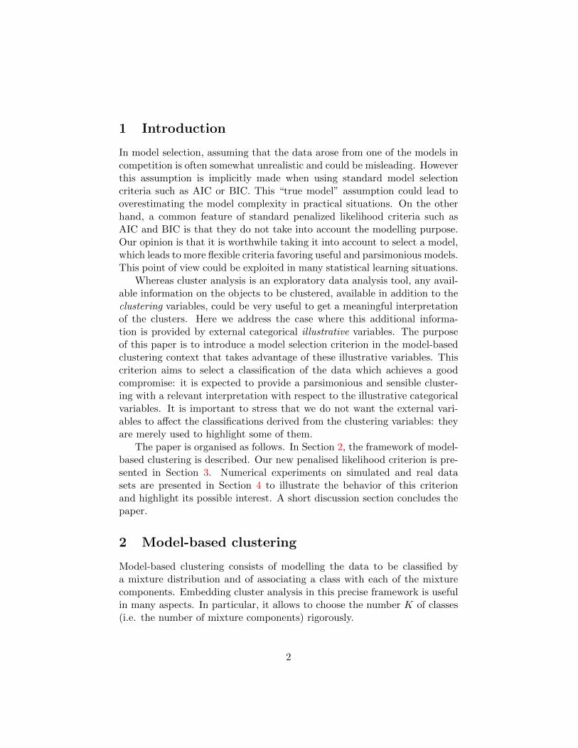
1 Introduction

In model selection, assuming that the data arose from one of the models incompetition is often somewhat unrealistic and could be misleading. Howeverthis assumption is implicitly made when using standard model selectioncriteria such as AIC or BIC. This “true model” assumption could lead tooverestimating the model complexity in practical situations. On the otherhand, a common feature of standard penalized likelihood criteria such asAIC and BIC is that they do not take into account the modelling purpose.Our opinion is that it is worthwhile taking it into account to select a model,which leads to more flexible criteria favoring useful and parsimonious models.This point of view could be exploited in many statistical learning situations.

Whereas cluster analysis is an exploratory data analysis tool, any avail-able information on the objects to be clustered, available in addition to theclustering variables, could be very useful to get a meaningful interpretationof the clusters. Here we address the case where this additional informa-tion is provided by external categorical illustrative variables. The purposeof this paper is to introduce a model selection criterion in the model-basedclustering context that takes advantage of these illustrative variables. Thiscriterion aims to select a classification of the data which achieves a goodcompromise: it is expected to provide a parsimonious and sensible cluster-ing with a relevant interpretation with respect to the illustrative categoricalvariables. It is important to stress that we do not want the external vari-ables to affect the classifications derived from the clustering variables: theyare merely used to highlight some of them.

The paper is organised as follows. In Section 2, the framework of model-based clustering is described. Our new penalised likelihood criterion is pre-sented in Section 3. Numerical experiments on simulated and real datasets are presented in Section 4 to illustrate the behavior of this criterionand highlight its possible interest. A short discussion section concludes thepaper.

2 Model-based clustering

Model-based clustering consists of modelling the data to be classified bya mixture distribution and of associating a class with each of the mixturecomponents. Embedding cluster analysis in this precise framework is usefulin many aspects. In particular, it allows to choose the number K of classes(i.e. the number of mixture components) rigorously.

2

2.1 Finite mixture models

Please refer to McLachlan and Peel (2000) for a comprehensive introductionto finite mixture models.

The data to be clustered y = (y1, . . . ,yn), with yi ∈ Rd, are modelledas observations of iid random variables with a mixture distribution:

f(y | θ) =n∏i=1

f(yi | θ) with f(yi | θ) =K∑k=1

pkφ(yi | ak)

where the pk’s are the mixing proportions and φ(· | ak) denotes the com-ponents probability density function (typically the d-dimensional Gaussiandensity) with parameter ak, and θ = (p1, . . . , pK−1,a1, . . . ,aK). A mix-ture model can be regarded as a latent structure model involving unknownlabel data z = (z1, . . . , zn) which are binary vectors with zik = 1 if andonly if yi arises from component k. Those indicator vectors define a par-tition P = (P1, . . . , PK) of the data y with Pk = {yi | zik = 1}. Howeverthese indicator vectors are not observed in a clustering problem: the modelis usually fitted through maximum likelihood estimation and an estimatedpartition is deduced from it by the MAP rule recalled in (1). The parame-ter estimator, denoted from now on by θ, is generally derived from the EMalgorithm (Dempster et al., 1977; McLachlan and Krishnan, 1997).

Remark that, for a given number of components K and a parameterθK , the class of each observation yi is assigned according to the MAP ruledefined above.

There are usually several models to choose among (typically, when thenumber of components is unknown). Note that a mixture model m is charac-terized not only by the number of components K, but also by assumptions onthe proportions and the component variance matrices (see Celeux and Gov-aert, 1995). The corresponding parameter space is denoted by Θm. From adensity estimation perspective, a classical way for choosing a mixture modelis to select the model maximising the integrated likelihood,

f(y | m) =

∫Θm

f(y | m, θm)π(θm)dθm,

π(θm) being a weakly informative prior distribution on θm. For n largeenough, it can be approximated with the BIC criterion (Schwarz, 1978)

log f(y | m) ≈ log f(y | m, θm)− νm2

log n,

3

with νm the number of free parameters in the mixture model m. Numericalexperiments (see for instance Roeder and Wasserman, 1997) and theoreticalresults (see Keribin, 2000) show that BIC works well to select the truenumber of components when the data actually arises from one of the mixturemodels in competition.

2.2 Choosing K from the clustering view point

In the model-based clustering context, an alternative to the BIC criterionis the ICL criterion (Biernacki et al., 2000) which aims at maximising theintegrated likelihood of the complete data (y, z)

f(y, z | m) =

∫Θm

f(y, z | m, θm)π(θm)dθm.

It can be approximated with a BIC-like approximation:

log f(y, z | m) ≈ log f(y, z | m, θ∗m)− νm2

log n

θ∗m = arg maxθm

f(y, z | m, θm).

But z and θ∗m are unknown. Arguing that θm ≈ θ∗m if the mixture compo-nents are well separated for n large enough, Biernacki et al. (2000) replaceθ∗m by θm and the missing data z with z = MAP(θm) defined by

zik =

{1 if argmax` τ

`i (θm) = k

0 otherwise,(1)

τki (θm) denoting the conditional probability that yi arises from the kth mix-ture component under θm (1 ≤ i ≤ n and 1 ≤ k ≤ K):

τki (θm) =pkφ(yi | ak)∑K`=1 p`φ(yi | a`)

. (2)

Finally the ICL criterion is

ICL(m) = log f(y, z | m, θm)− νm2

log n. (3)

Roughly speaking ICL is the criterion BIC decreased by the estimated meanentropy

E(m) = −K∑k=1

n∑i=1

τki (θm) log τki (θm) ≥ 0.

4

This is apparent if the estimated labels z are replaced in the definition (3)by their respective conditional expectation τki (θm), since log f(y, z|m, θm) =log f(y|m, θm) +

∑ni=1

∑Kk=1 zik log τki (θm).

Because of this additional entropy term, ICL favors models which leadto partitioning the data with the greatest evidence. The derivation and ap-proximations leading to ICL are questioned in Baudry (2009, Chapter 4).However, in practice, ICL appears to provide a stable and reliable estimateof the number of mixture components for real data sets and also for simu-lated data sets from the clustering view point. ICL, which is not aiming atdiscovering the true number of mixture components, can underestimate thenumber of components for simulated data arising from mixtures with poorlyseparated components (Biernacki et al., 2000). It concentrates on selectinga relevant number of classes.

3 A particular clustering selection criterion

Now, suppose that, beside y, a known classification u (e.g. associated to anextra categorical variable) is available. We still want to build a classificationz based on y, which is supposed to carry some more information than u. Butrelating the classifications z and u could be of interest to get a suggestive andsimple interpretation of z. Therefore, we propose to build the classification zin each model, based on y only, but to involve u in the model selection step.Hopefully u might highlight some of the solutions among which y wouldnot enable to decide clearly. This might help to select a model providing agood compromise between the mixture model fit to the data and its abilityto lead to a classification of the observations well related to the externalclassification u. To derive our heuristics, we suppose that y and u areconditionally independent knowing z, which means that all the relevantinformation in u and y can be caught by z. This is for example true inthe very particular case where u can be written as a function of z: u is areduction of the information included in z, and we hope to be able to retrievemore information from u using the (conditionally independent) informationbrought by y.

Here is our heuristics. It is based on an intent to find the mixture modelmaximizing the integrated completed likelihood

f(y,u, z | m) =

∫f(y,u, z | m, θm)π(θm)dθm. (4)

Assuming that y and u are conditionally independent knowing z, whichshould hold at least for models with enough components, it can be written

5

for any θm ∈ m:

f(y,u, z|m, θm) = f(y, z|m, θm) f(u|y, z,m, θm)︸ ︷︷ ︸f(u|z,m,θm)

. (5)

But neither θm nor m carry any information on the model for u|z and thenf(u|z,m, θm) = f(u|z). Let us denote (nk`)1≤`≤U,1≤k≤K the contingencytable relating the categorical variables u and z: for any k ∈ {1, . . . ,K} and` ∈ {1, . . . , U}, U being the number of levels of the variable u,

nk` = card{i|zik = 1 and ui = `

}.

Moreover, let us denote nk. =∑U

`=1 nk`. Denoting

L ={

(qk`)1≤`≤U1≤k≤K

∈ (0, 1)K×U |∀k ∈ {1, . . . ,K},U∑`=1

qk` = 1},

we have

argmax(qk`)∈L

n∑i=1

log qziui =(nk`nk.

)1≤`≤U1≤k≤K

.

Thus, we get

log f(u | z) =n∑i=1

lognziuinzi.

=

U∑`=1

K∑k=1

nk` lognk`nk.

and, from (4) and (5),

log f(y,u, z | m) =

U∑`=1

K∑k=1

nk` lognk`nk.

+ log

∫f(y, z | m, θm)π(θm)dθm.

Now, log∫f(y, z | m, θm)π(θm)dθm can be approximated by ICL as in (3).

Thus

log f(y,u, z | m) ≈ log f(y, z | m, θm) +

U∑`=1

K∑k=1

nk` lognk`nk.− νm

2log n.

6

Finally, this leads to the Supervised Integrated Completed Likelihood(SICL) criterion

SICL(m) = ICL(m) +U∑`=1

K∑k=1

nk` lognk`nk·

.

The last additional term∑U

`=1

∑Kk=1 nk` log nk`

nk·quantifies the strength of

the link between the categorical variables u and z. This might be helpfuleventually for the interpretation of the classification z.

Taking several external variables into account The same kind ofderivation enables to derive a criterion that takes into account several ex-ternal variables u1, . . . ,ur. Suppose that y,u1, . . . ,ur are conditionally in-dependent knowing z. Then (5) becomes

f(y,u1, . . . ,ur, z | m, θ∗m) = f(y, z | m, θ∗m)

× f(u1 | y, z,m, θ∗m)︸ ︷︷ ︸f(u1|z,m,θ∗m)

× . . .× f(ur | y, z,m, θ∗m)︸ ︷︷ ︸

f(ur|z,m,θ∗m)

,

(6)

with θ∗m = arg maxθm f(y,u1, . . . ,ur, z | m, θm). As before, we assume thatθm ≈ θ∗m and apply the BIC-like approximation. Finally,

log f(y,u1, . . . ,ur, z | m) ≈ log f(y, z | m, θm)

+ log f(u1 | z,m, θm)

+ . . .

+ log f(ur | z,m, θm)

− νm2

log n,

and as before, log f(uj | z) = log f(uj | z,m, θm) is derived from the con-tingency table (njk`) relating the categorical variables uj and z: for anyk ∈ {1, . . . ,K} and ` ∈ {1, . . . , U j}, U j being the number of levels of thevariable uj,

njk` = card{i|zik = 1 and uji = `

}.

7

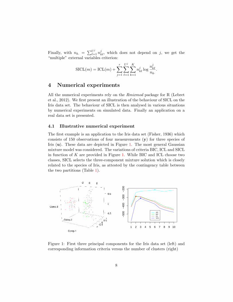
Finally, with nk. =∑Uj

`=1 njk`, which does not depend on j, we get the

“multiple” external variables criterion:

SICL(m) = ICL(m) +r∑j=1

Uj∑`=1

K∑k=1

njk` lognjk`nk·

.

4 Numerical experiments

All the numerical experiments rely on the Rmixmod package for R (Lebretet al., 2012). We first present an illustration of the behaviour of SICL on theIris data set. The behaviour of SICL is then analysed in various situationsby numerical experiments on simulated data. Finally an application on areal data set is presented.

4.1 Illustrative numerical experiment

The first example is an application to the Iris data set (Fisher, 1936) whichconsists of 150 observations of four measurements (y) for three species ofIris (u). These data are depicted in Figure 1. The most general Gaussianmixture model was considered. The variations of criteria BIC, ICL and SICLin function of K are provided in Figure 1. While BIC and ICL choose twoclasses, SICL selects the three-component mixture solution which is closelyrelated to the species of Iris, as attested by the contingency table betweenthe two partitions (Table 1).

Number of Clusters

1 2 3 4 5 6 7 8 9 10

−50

0−

400

−30

0−

200

AICBICICLSICL

Figure 1: First three principal components for the Iris data set (left) andcorresponding information criteria versus the number of clusters (right)

8

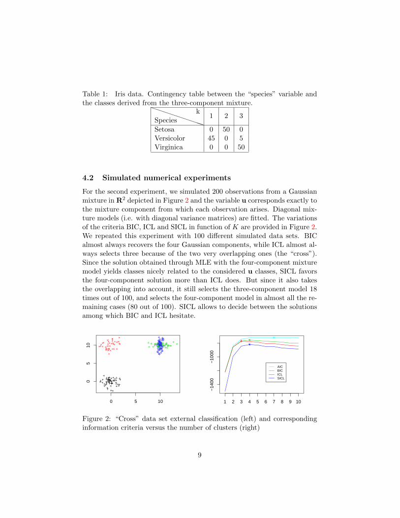
Table 1: Iris data. Contingency table between the “species” variable andthe classes derived from the three-component mixture.

PPPPPPPPPSpeciesk

1 2 3

Setosa 0 50 0Versicolor 45 0 5Virginica 0 0 50

4.2 Simulated numerical experiments

For the second experiment, we simulated 200 observations from a Gaussianmixture in R2 depicted in Figure 2 and the variable u corresponds exactly tothe mixture component from which each observation arises. Diagonal mix-ture models (i.e. with diagonal variance matrices) are fitted. The variationsof the criteria BIC, ICL and SICL in function of K are provided in Figure 2.We repeated this experiment with 100 different simulated data sets. BICalmost always recovers the four Gaussian components, while ICL almost al-ways selects three because of the two very overlapping ones (the “cross”).Since the solution obtained through MLE with the four-component mixturemodel yields classes nicely related to the considered u classes, SICL favorsthe four-component solution more than ICL does. But since it also takesthe overlapping into account, it still selects the three-component model 18times out of 100, and selects the four-component model in almost all the re-maining cases (80 out of 100). SICL allows to decide between the solutionsamong which BIC and ICL hesitate.

●● ●●

●

●

●●

●●●

●

●

●● ●

●

●●

●

●

●

●●

● ●

●

●● ●

●●

●●

●

●●

●●

●●●

●●

●

0 5 10

05

10

Number of Clusters

1 2 3 4 5 6 7 8 9 10

−14

00−

1000

AICBICICLSICL

Figure 2: “Cross” data set external classification (left) and correspondinginformation criteria versus the number of clusters (right)

9

The third experiment illustrates a situation where SICL gives a relevantsolution different from the solutions selected with BIC and ICL. We sim-ulated 200 observations of a diagonal three-component Gaussian mixturedepicted in Figure 3 where the classes of u are in red and in black. (Thered class is composed of two “horizontal” Gaussian components while theblack one is composed of a single “vertical” Gaussian component...) Themost general Gaussian mixture model was considered. From Table 2 BICalmost always recovers the three components of the simulated mixture, ICLmostly selects one cluster, and SICL chooses two classes well related to u.

−2 0 2 4 6 8

−2

02

46

Number of Clusters

1 2 3 4 5 6 7 8 9 10

−31

00−

2900

−27

00−

2500

AICBICICLSICL

Figure 3: Third experiment data set external classification (left) and corre-sponding information criteria versus the number of clusters (right)

Table 2: Number of components selected by each criterion for the thirdexperiment data

K 1 2 3 4 5 6 7 8 9 10

AIC 0 0 24 26 20 8 6 4 5 7BIC 0 4 96 0 0 0 0 0 0 0ICL 53 44 3 0 0 0 0 0 0 0SICL 0 86 14 0 0 0 0 0 0 0

In the next two experiments, we analyse the behaviour of SICL in situ-ations where u cannot be related with the mixture distributions at hand.

At first we consider a situation where u is a two-class partition whichhas no link at all with a four-component mixture data. Diagonal mixturemodels are fitted. In Figure 4 the classes of u are in red and in black. As isapparent from Figure 4, SICL does not change the solution K = 4 providedby BIC and ICL.

10

0 5 10

05

10

Number of Clusters

1 2 3 4 5 6 7 8 9 10

−13

00−

1100

−90

0

AICBICICLSICL

Figure 4: “Random labels” data set external classification (left) and corre-sponding information criteria versus the number of clusters (right)

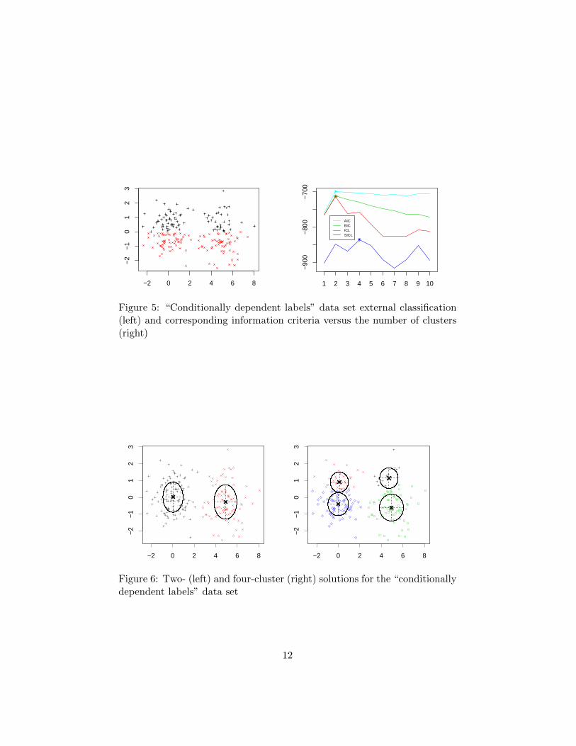
About the conditional independence assumption The heuristics lead-ing to SICL assumes that u and y are independent conditionally on z (seeSection 3). This assumption is questionable and might not hold for all theconsidered models. The next experiment aims at studying the behaviourof SICL when it can be regarded as inappropriate. We consider a two-component diagonal mixture and a two-class u partition “orthogonal” tothis mixture. In Figure 5 the classes of u are in red and in black. Diag-onal mixture models with free volumes and proportions but fixed shapesand orientations are fitted (see Celeux and Govaert, 1995). As is apparentfrom Figure 5 and Table 3, SICL highlights the two- and the four-clustersolutions. Actually the conditional independence does not hold for the twocluster solution but it does for the four cluster solution (see Figure 6) whichis of interest when the focus is on the link between z and u. However it isclear from the dispersion of the numbers of clusters selected with SICL (Ta-ble 3) that this criterion is jeopardized when the conditional independencedoes not hold for the relevant numbers of clusters.

Table 3: Number of components selected by each criterion for the “Condi-tionally dependent labels” data.

K 1 2 3 4 5 6 7 8 9 10

AIC 0 47 24 14 4 4 2 0 4 1BIC 0 99 1 0 0 0 0 0 0 0ICL 0 100 0 0 0 0 0 0 0 0SICL 0 36 10 19 7 6 5 6 7 4

11

−2 0 2 4 6 8

−2

−1

01

23

Number of Clusters

1 2 3 4 5 6 7 8 9 10

−90

0−

800

−70

0

AICBICICLSICL

Figure 5: “Conditionally dependent labels” data set external classification(left) and corresponding information criteria versus the number of clusters(right)

−2 0 2 4 6 8

−2

−1

01

23

−2 0 2 4 6 8

−2

−1

01

23

Figure 6: Two- (left) and four-cluster (right) solutions for the “conditionallydependent labels” data set

12

4.3 Real data set: wholesale customers

The segmentation of customers of a wholesale distributor is performed toillustrate the performance of the SICL criterion. The data set refers to 440customers of a wholesale: 298 from the Horeca (Hotel/Restaurant/Cafe)channel and 142 from the Retail channel. They are distributed into twolarge Portuguese city regions (Lisbon and Oporto) and a complementaryregion.

Table 4: Distribution of the Region variableRegion Frequency PercentageLisbon 77 17.5Oporto 47 10.5

Other region 316 31.8Total 440 100

The wholesale data concern customers. They include the annual spend-ing in monetary units (m.u.) on product categories: fresh products, milkproducts, grocery, frozen products, detergents and paper products, and del-icatessen. These variables are summarized in Table 5.

Table 5: Product categories sales (m.u.).Mean Std. Deviation

Fresh products 12000 12647Milk products 5796 5796

Grocery 7951 9503Frozen 3072 4855

Detergents and Paper 2881 4768Delicatessen 1525 2820

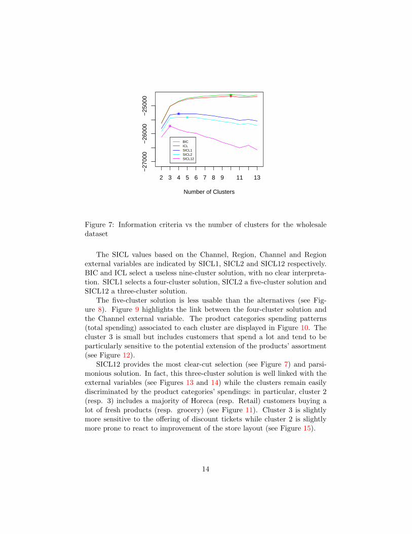
These data also include responses to a questionnaire intended to evaluatepossible managerial actions with potential impact on sales such as improvingthe store layout, offering discount tickets or extending products’ assortment.The customers were asked whether the referred action would have impacton their purchases in the wholesale and their answers were registered in thescale: 1-Certainly no; 2-Probably no; 3-Probably yes; 4-Certainly yes. Diag-onal mixture models have been fitted on the continuous variables describedin Table 5. The results are presented in Figure 7.

13

Number of Clusters

2 3 4 5 6 7 8 9 11 13

−27

000

−26

000

−25

000

BICICLSICL1SICL2SICL12

Figure 7: Information criteria vs the number of clusters for the wholesaledataset

The SICL values based on the Channel, Region, Channel and Regionexternal variables are indicated by SICL1, SICL2 and SICL12 respectively.BIC and ICL select a useless nine-cluster solution, with no clear interpreta-tion. SICL1 selects a four-cluster solution, SICL2 a five-cluster solution andSICL12 a three-cluster solution.

The five-cluster solution is less usable than the alternatives (see Fig-ure 8). Figure 9 highlights the link between the four-cluster solution andthe Channel external variable. The product categories spending patterns(total spending) associated to each cluster are displayed in Figure 10. Thecluster 3 is small but includes customers that spend a lot and tend to beparticularly sensitive to the potential extension of the products’ assortment(see Figure 12).

SICL12 provides the most clear-cut selection (see Figure 7) and parsi-monious solution. In fact, this three-cluster solution is well linked with theexternal variables (see Figures 13 and 14) while the clusters remain easilydiscriminated by the product categories’ spendings: in particular, cluster 2(resp. 3) includes a majority of Horeca (resp. Retail) customers buying alot of fresh products (resp. grocery) (see Figure 11). Cluster 3 is slightlymore sensitive to the offering of discount tickets while cluster 2 is slightlymore prone to react to improvement of the store layout (see Figure 15).

14

Figure 8: Distribution of the vari-able Region on the SICL2 solution

Figure 9: Distribution of the vari-able Channel on the SICL1 solution

Figure 10: Distribution of the prod-uct categories on the SICL1 solution

Figure 11: Distribution of the prod-uct categories on the SICL12 solu-tion

15

Figure 12: SICL1 solution and managerial actions

Figure 13: Distribution of the Chan-nel variable on the SICL12 solution

Figure 14: Distribution of the Re-gion variable on the SICL12 solution

16

Figure 15: SICL12 solution and managerial actions

5 Discussion

The criterion SICL has been conceived in the model-based clustering contextto choose a sensible number of classes, possibly taking advantage of an exter-nal categorical variable or a set of external categorical variables of interest(variables other than the variables on which the clustering is based). Thiscriterion can be useful to draw attention to a well-grounded classificationrelated to this external categorical variables.

In mixture analysis several authors propose to make the mixing propor-tions depend on covariates through logistic models (see for example Daytonand Macready, 1988). However, to the best of our knowledge, there wereno works relying on the point of view of SICL in model selection: to selectthe model with the help of external variables which are not used to fit eachmodel.

As one of the referees noticed, it may be possible to get the same solutionas SICL by including the illustrative variables in the model, as it is the casefor example for the Iris data set. But not including them in the modelprovides a stronger evidence of the link between the illustrative variablesand the clustering for the very reason that the illustrative variables are notinvolved in the design of the clustering.

A possible limitation of SICL is the conditional independence assumptionon which its heuristics rely (see Section 3). The simulation study describedat the end of Section 4.2 illustrates the situation where u is not conditionallyindependent on y given z for the number of clusters selected by BIC orICL. In such a case SICL could highlight clusterings for which u and y areconditionally independent and tends to select a model with a higher number

17

of clusters than BIC and ICL. Indeed SICL tends to select a model in which zsummarizes the information brought both by u and y. It could be expectedto be far from the clusterings provided by standard model selection criteriabut in doing so SICL points out a sensible and interesting solution.

Section 4.3 and experiments not reported here suggest that the higherthe number of external variables the greater the interest of SICL.

Finally SICL could highlight partitions of special interest with respectto external categorical variables. Therefore, we think that SICL deservesto enter in the toolkit of model selection criteria for clustering. In mostcases, it will propose a sensible solution and when it points out an originalsolution, it could be of great interest for practical purposes.

18

References

Baudry, J.-P. (2009). Model Selection for Clustering. Choosing theNumber of Classes. PhD thesis, Univ. Paris-Sud. http://tel.

archives-ouvertes.fr/tel-00461550/fr/.

Biernacki, C., Celeux, G., and Govaert, G. (2000). Assessing a mixturemodel for clustering with the integrated completed likelihood. IEEETrans. PAMI, 22:719–725.

Biernacki, C., Celeux, G., Govaert, G., and Langrognet, F. (2006). Model-based cluster and discriminant analysis with the mixmod software. Com-putational Statistics and Data Analysis, 51(2):587–600.

Celeux, G. and Govaert, G. (1995). Gaussian parsimonious clustering mod-els. Pattern Recognition, 28(5):781 – 793.

Dayton, C. M. and Macready, G. B. (1988). Concomitant-variablelatent-class models. Journal of the American Statistical Association,83(401):173–178.

Dempster, A., Laird, N., and Rubin, D. (1977). Maximum likelihood fromincomplete data via the EM-algorithm. Journal of the Royal StatisticalSociety. Series B, 39(1):1–38.

Fisher, R. (1936). The use of multiple measurements in taxonomic problems.Annals of Eugenics, 7:179–188.

Keribin (2000). Consistent estimation of the order of mixture models.Sankhya A, 62(1):49–66.

Lebret, R., Iovleff, S., Langrognet, F., Biernacki, C., Celeux, G., and Go-vaert, G. (2012). Rmixmod: The r package of the model-based unsu-pervised, supervised and semi-supervised classification mixmod library.http://cran.r-project.org/web/packages/Rmixmod/index.html.

McLachlan, G. and Krishnan, T. (1997). The EM-algorithm and Extensions.New York : Wiley.

McLachlan, G. and Peel, D. (2000). Finite Mixture Models. New York :Wiley.

Roeder, K. and Wasserman, L. (1997). Practical bayesian density estimationusing mixtures of normals. Journal of the American Statistical Associa-tion, 92(439):894–902.

19

Schwarz, G. (1978). Estimating the dimension of a model. Ann. Statist.,6:461–464.

20

Jean-Patrick BaudryUniversite Pierre et Marie Curie - Paris VIBoıte 158, Tour 15-25, 2e etage4 place Jussieu, 75252 Paris Cedex 05France.Jean-Patrick.Baudry@upmc.frhttp://www.lsta.upmc.fr/Baudry

21