Embed Size (px)
Citation preview

Enhanced Thermal Conductivity and Expedited Freezing of Nanoparticle Suspensions
Utilized as Novel Phase Change Materials
by
Liwu Fan
A dissertation submitted to the Graduate Faculty of
Auburn University
in partial fulfillment of the
requirements for the Degree of
Doctor of Philosophy
Auburn, Alabama
August 6, 2011
Keywords: Freezing, Nanoparticle Suspensions, Phase Change Materials, Transient Plane
Source Technique, Thermal Conductivity Enhancement, Thermal Energy Storage
Copyright 2011 by Liwu Fan
Approved by
Jay M. Khodadadi, Chair, Alumni Professor of Mechanical Engineering
W. Robert Ashurst, Associate Professor of Chemical Engineering
Daniel W. Mackowski, Associate Professor of Mechanical Engineering
Amnon J. Meir, Professor of Mathematics and Statistics
ii
Abstract
In this dissertation, enhanced thermal conductivity and expedited freezing of nanoparticle
suspensions used as novel phase change materials (PCM), referred to as nano-enhanced PCM
(NePCM), were investigated using analytic, experimental and numerical methods.
Two hydrocarbons, cyclohexane (C6H12) and eicosane (C20H42), were selected as the base
PCM. Copper oxide (CuO) nanoparticles, stabilized by sodium oleate acid (SOA), were used as
the nano-structured thermal conductivity enhancers. Thermal conductivity measurements using
the transient plane source (TPS) technique were performed for the NePCM samples in both
liquid and solid phases. The dependence of thermal conductivity on both temperature and the
loading of CuO nanoparticles was investigated. In the liquid phase, thermal conductivity
enhancement was clearly observed with increasing loading of nanoparticles, and was found to be
in good agreement with the predicted values of the Maxwell’s equation. The measured thermal
conductivity enhancement in the solid phase, however, exhibited a non-monotonic enhancement
phenomenon for both cyclohexane- and eicosane-based samples for mass fraction of
nanoparticles greater than 2 percent.
Mathematical modeling of unidirectional freezing of NePCM was conducted through a one-
dimensional, two-region Stefan problem, in which the NePCM was treated as a ―single-phase‖
PCM with modified effective thermophysical properties in the presence of nanoparticles. The
problem was solved by employing both a combined analytic/integral approach and the extended
lattice Boltzmann method (LBM) with enthalpy formulation. The analytic solution was then

iii
applied to two representative cases of aqueous and cyclohexane-based NePCM with various
metal and metal oxide nanoparticles. It was clearly shown that freezing is expedited as the
loading of nanoparticles is increased. For example, expediting of freezing of water was observed
to be up to 11.4 percent by introducing nanoparticles at a volume fraction of 10 percent.
In an effort to validate the expedited unidirectional freezing observed through mathematical
modeling, a cooled-from-bottom freezing experimental setup was designed and constructed. The
cooling boundary was first realized by utilizing a thermoelectric cooler (TEC). Due to the lack of
boundary temperature control, the experimental results on freezing of cyclohexane-based
NePCM samples exhibited great discrepancies with the numerical predictions based on the
Stefan model. The experimental setup was then refined by replacing the TEC with a copper cold
plate (CCP). With the aid of a controllable constant-temperature bath, a stable cold boundary
condition was achieved. It was observed that the experimental results from the improved setup
were in good agreement with the numerical predictions. The greatest expediting (5.2 percent) of
freezing of cyclohexane was realized experimentally by introducing CuO nanoparticles with a
mass fraction of 2 percent.
Having shown the enhanced thermal conductivity and expedited unidirectional freezing of
hydrocarbon-based NePCM samples, the great potential of such novel materials with
applications to improved thermal energy storage and waste heat recovery was justified. Further
effort of NePCM research will be devoted to improving the colloidal stability, measuring the
thermophysical properties for various colloids, and investigating melting heat transfer that will
involve natural convection. Mathematical modeling and experimental investigation of microscale
dynamics of nanoparticles in suspensions undergoing phase change are also challenging.

iv
Acknowledgments
I would like to sincerely thank my advisor, Dr. Jay M. Khodadadi, for his supervision,
support, understanding, encouragement and friendship during the entire course of my doctoral
study at Auburn University. In addition to his insightful mentorship that was paramount in
guiding my doctoral explorations on the right track toward achieving the research objectives, he
also extended initiatively to me a great number of opportunities to accumulate academic and
professional experience consistent my long-term career goals. I would also like to thank all of
my current and former group members, Hasan Babaei, Tatyana Bodrikova, Yousef El-Hasadi,
Mahmoud Moeini Sedeh and Alex Scammell, for providing me with timely assistance and
valuable inspiration, as well as maintaining a relaxed and interactive laboratory environment.
Consecutive financial support for my dissertation work provided by the Graduate Research
Scholars Program (GRSP) of the Alabama Experimental Program to Stimulate Competitive
Research (EPSCoR) through rounds 5 and 6 is gratefully acknowledged.
I would like to thank Dan Clary and Dr. German Mills of the Department of Chemistry and
Biochemistry for supplying the synthesized nanoparticles and guiding the preparation,
characterization and testing of the colloidal suspensions. I would also like to thank John Maddox
and Naveenan Thiagarajan of the Department of Mechanical Engineering for their valuable
discussions on experimental techniques and instrumentation for measuring temperature. Many
thanks are also due to John Montgomery of the Glass Shop of the Department of Chemistry and
Biochemistry for his hard work and expertise in fabricating customized glass apparatus.

v
I would like to thank Doctors W. Robert Ashurst, Daniel W. Mackowski and Amnon J. Meir
of the Departments of Chemical Engineering, Mechanical Engineering and Mathematics and
Statistics, respectively, for serving as the committee members. In particular, the knowledge I
gained from the graduate courses taught by them was key to my doctoral research. Special thanks
also go to Dr. Jong Wook Hong of the Department of Materials Engineering for serving as the
outside reader of my dissertation.
I am very grateful for the friendship of all of my colleagues and friends in the Auburn family,
especially my roommate Rong Jiang, who made my stay at Auburn a memorable experience.
Finally and most importantly, I would like to thank my wife Wei (Vivian) Zhang, my parents and
parents-in-law. Without their unending love, encouragement, understanding and patience, I
would never have the chance to finish this dissertation.
Permission to reuse copyrighted materials in compilation of this dissertation granted by
Elsevier and the American Society of Mechanical Engineers (ASME) is acknowledged. These
materials include:
1) Liwu Fan and J. M. Khodadadi, 2011, Thermal conductivity enhancement of phase
change materials for thermal energy storage: a review, Renewable and Sustainable
Energy Reviews, vol. 15, pp. 24-46 (in Chapter 2),
2) J. M. Khodadadi and Liwu Fan, Expedited freezing of nanoparticle-enhanced phase
change materials (NEPCM) exhibited through a simple 1-D Stefan problem formulation,
Proceedings of the ASME 2009 Summer Heat Transfer Conference, Paper No. HT2009-
88409, pp. 345-351 (in Chapter 4), and
3) Liwu Fan and J. M. Khodadadi, Experimental verification of expedited freezing of
nanoparticle-enhanced phase change materials (NEPCM), Proceedings of the

vi
ASME/JSME 2011 8th
Thermal Engineering Joint Conference, Paper No. AJTEC2011-
44165, pp. T10221-7 (in Chapter 5).
This dissertation is based upon work partially supported by the US Department of Energy
under Award Number DE-SC0002470. This report was prepared as an account of work
sponsored by an agency of the United States Government. Neither the United States Government
nor any agency thereof, nor any of their employees makes any warranty, express or implied, or
assumes any legal liability or responsibility for the accuracy, completeness, or usefulness of any
information, apparatus, product, or process disclosed, or represents that its use would not
infringe privately owned rights. Reference herein to any specific commercial product, process, or
service by trade name, trademark, manufacturer, or otherwise does not necessarily constitute or
imply its endorsement, recommendation, or favoring by the Unites States Government or any
agency thereof. The views and opinions of authors expressed herein do not necessarily state or
reflect those of the United States Government or any agency thereof.

vii
Table of Contents
Abstract ........................................................................................................................................... ii
Acknowledgments.......................................................................................................................... iv
List of Tables ................................................................................................................................. xi
List of Figures .............................................................................................................................. xiii
List of Symbols .......................................................................................................................... xviii
Chapter 1 Introduction ................................................................................................................... 1
1.1 Background and Motivation .............................................................................................. 1
1.2 Research Objectives and Methodology ............................................................................. 4
1.3 Outline of the Dissertation ................................................................................................. 5
Chapter 2 Literature Survey ........................................................................................................... 8
2.1 Thermal Conductivity Enhancement of PCM Through Fixed Structures ......................... 8
2.1.1 Early work related to heat rejection issues in space exploration systems................. 9
2.1.2 Extension to solar thermal and thermal management of electronics ...................... 11
2.2 Nano-Enhanced PCM (NePCM)...................................................................................... 24
2.2.1 Early work on meso- to micro-scale enhancers ...................................................... 24
2.2.2 Enhancement using nano-structured materials ....................................................... 26
2.3 Prediction of the Effective Thermal Conductivity of Two-Phase Mixtures .................... 31
2.4 Summary .......................................................................................................................... 34

viii
Chapter 3 Preparation of NePCM Colloids and Measurement of Their Thermal Conductivity . 80
3.1 Preparation of Hydrocarbon-Based NePCM Colloids ..................................................... 80
3.1.1 Selection of base PCM and concern of colloidal stability ...................................... 80
3.1.2 Preparation of hydrocarbon-based NePCM with stabilized CuO nanoparticles ..... 82
3.2 Measurement of Thermal Conductivity ........................................................................... 84
3.2.1 Instrument and principle of the transient plane source (TPS) technique ................ 84
3.2.2 Experimental setup and procedure .......................................................................... 87
3.2.3 Verification of accuracy and reproducibility of the TPS instrument ...................... 89
3.3 Results and Discussion .................................................................................................... 90
3.3.1 Cyclohexane-based NePCM samples ..................................................................... 90
3.3.2 Eicosane-based NePCM samples ............................................................................ 91
3.3.3 Improved measurement of eicosane-based NePCM samples in solid phase .......... 95
3.4 Summary .......................................................................................................................... 96
Chapter 4 Mathematical Modeling of Expedited Unidirectional Freezing of NePCM ............. 113
4.1 One-Dimensional Two-Region Stefan Problem ............................................................ 113
4.1.1 Fundamental assumptions for the Stefan problem ................................................ 113
4.1.2 Physical model for freezing of NePCM ................................................................ 115
4.1.3 Mathematical formulation ..................................................................................... 116
4.2 Combined Analytic and Integral Method ...................................................................... 118
4.2.1 Analytic solution in the frozen layer ..................................................................... 119
4.2.2 Integral solution in the liquid layer ....................................................................... 119
4.2.3 Numerical solution for the interfacial condition ................................................... 120

ix
4.3 Lattice Boltzmann Method (LBM) ................................................................................ 121
4.3.1 Principle of the LBM for fluid flow ...................................................................... 121
4.3.2 Thermal LBM (TLBM)......................................................................................... 125
4.3.3 Extended TLBM for heat conduction with phase change ..................................... 127
4.3.4 The LBM solution for the 1-D Stefan problem .................................................... 129
4.4 Prediction of the Effective Thermophysical Properties of NePCM ............................... 133
4.5 Application of the Analytic Solution ............................................................................. 134
4.5.1 Thermophysical properties and parameters .......................................................... 134
4.5.2 Effect of the liquid to solid thermal conductivity ratio ......................................... 135
4.5.3 Effect of the liquid to solid thermal diffusivity ratio ............................................ 136
4.5.4 Expedited freezing rate ......................................................................................... 137
4.6 Summary ........................................................................................................................ 138
Chapter 5 Experimental Investigations of Expedited Unidirectional Freezing of NePCM ....... 156
5.1 Unidirectional Freezing Experiment: A Test Case with Distilled Water ...................... 156
5.1.1 Experimental setup and instruments ..................................................................... 156
5.1.2 Experiment on ice formation ................................................................................ 159
5.1.3 Results and discussion .......................................................................................... 160
5.2 Experiment on NePCM Using a Thermoelectric Cooler (TEC) .................................... 161
5.2.1 Experimental details and procedure ...................................................................... 161
5.2.2 Experimental results and comparison with the 1-D Stefan problem .................... 163
5.2.3 Sources of discrepancies ....................................................................................... 165
5.3 Improved Experiment on NePCM Using a Copper Cold Plate (CCP) .......................... 167

x
5.3.1 Improvements relative to the previous work ........................................................ 167
5.3.2 Experimental setup and procedure ........................................................................ 168
5.3.3 Results and discussion .......................................................................................... 170
5.4 Summary ........................................................................................................................ 172
Chapter 6 Conclusions and Perspectives ................................................................................... 194
6.1 Concluding Remarks ...................................................................................................... 194
6.2 Suggestions for Future Work ......................................................................................... 196
Bibliography ............................................................................................................................... 198
Appendix A MATLAB Code for Numerical Root-Finding ...................................................... 211
Appendix B MATLAB Code for Implementing the LBM Solution.......................................... 214
Appendix C Predicted Thermophysical Properties of NePCM Samples ................................... 218
Appendix D Calibration of Thermocouples ............................................................................... 225
Appendix E LabVIEW Virtual Instrument for Data Acquisition of Thermocouples ................ 228
Appendix F Uncertainty Analysis of the Experimental Results ................................................ 230
Appendix G Estimation of Time Response of Thermocouples ................................................. 231

xi
List of Tables
Table 2.1 Summary of the reviewed studies on thermal conductivity enhancement of PCM
through fixed structures (Fan and Khodadadi, 2011) .............................................. 36
Table 2.2 Summary of the configurations of experimental setups and thermal operating
conditions of the reviewed studies (Fan and Khodadadi, 2011) .............................. 49
Table 2.3 Summary of the base PCM and nano-structured materials considered in the
published NePCM articles ....................................................................................... 53
Table 2.4 Summary of preparation and characterization methods and instruments in the
published NePCM articles ....................................................................................... 58
Table 3.1 Density, latent heat of fusion and phase change temperatures of cyclohexane and
eicosane in their liquid phase ................................................................................... 98
Table 3.2 Specifications of the Hot Disk Thermal Constants Analyser (TPS 500) ................. 99
Table 3.3 Measured thermal conductivity (unit: W/mK) of purified water at room temperature
and atmospheric pressure ....................................................................................... 100
Table 3.4 Measured thermal conductivity (unit: W/mK) of eicosane-based NePCM samples in
solid phase.............................................................................................................. 101
Table 4.1 Parameters in the ice formation problem for validating the LBM solution ........... 140
Table 4.2 Predicted dimensionless total freezing times and the corresponding percentages of
expediting (in parentheses) for aqueous and cyclohexane-based NePCM ............ 141
Table 5.1 The experimental parameters of the TEC setup imposed for the 1-D Stefan problem
............................................................................................................................... 175
Table 5.2 Comparison of the experimental and numerical results of the elapsed times for the
freezing front to reach the height of 12.6 mm ....................................................... 176
Table 5.3 Comparison of the measured elapsed freezing times (unit: second) for the frozen

xii
layer to reach various TC levels utilizing the original TEC and the improved CCP
setups for pure cyclohexane ................................................................................... 177
Table 5.4 Adopted thermal conductivity (unit: W/mK) from measurements of both liquid and
solid cyclohexane-based NePCM samples with various loadings of nanoparticles
............................................................................................................................... 178
Table 5.5 The experimental parameters for the improved experimental setup using a CCP
utilized for the 1-D Stefan problem ....................................................................... 179
Table 5.6 Comparison between the observed and predicted elapsed times to form a 7.3 mm thick
frozen layer of NePCM ........................................................................................... 180
Table C.1 Thermophysical properties of water (ice) and cyclohexane .................................. 219
Table C.2 Thermophysical properties of bulk materials for the nanoparticles considered (Jang
and Choi, 2007)...................................................................................................... 220
Table C.3 Predicted thermophysical properties of water-based NePCM with various
nanoparticles in the liquid phase ............................................................................ 221
Table C.4 Predicted thermophysical properties of water-based NePCM with various
nanoparticles in the solid phase ............................................................................. 222
Table C.5 Predicted thermophysical properties of cyclohexane-based NePCM with various
nanoparticles in the liquid phase ............................................................................ 223
Table C.6 Predicted thermophysical properties of cyclohexane-based NePCM with various
nanoparticles in the solid phase ............................................................................. 224
Table D.1 The measured temperature shifts of the eight (8) TCs against 0 °C ...................... 226

xiii
List of Figures
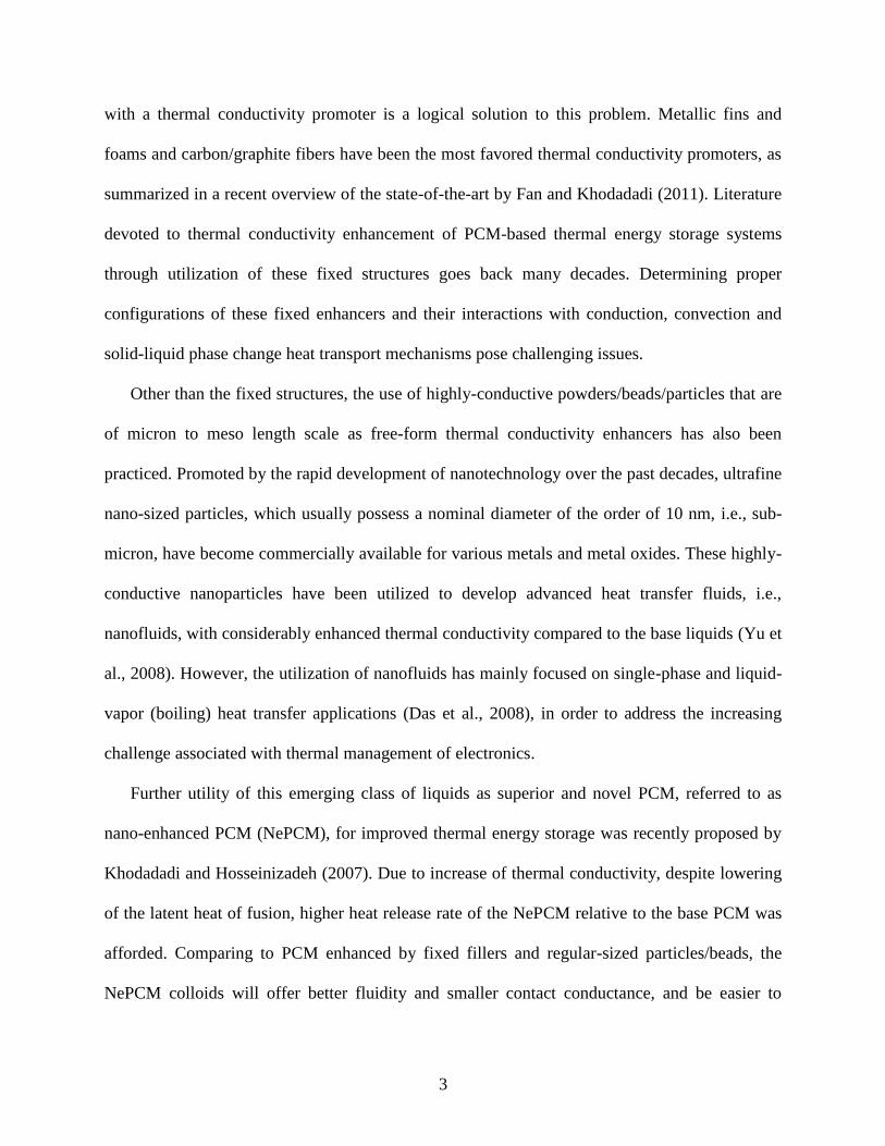
Figure 1.1 Storage capacity and discharge feature of various forms of energy storage units
(reproduced from Hammerschlag and Schaber, 2008) .............................................. 6
Figure 1.2 Typical groups of materials used as PCM and their latent heats versus melting
temperatures (reproduced from Mehling and Cabeza, 2007) .................................... 7
Figure 2.1 Schematic diagram of the experimental setup of the honeycomb-packed PCM
capacitor (reproduced from Abhat, 1976) ................................................................ 63
Figure 2.2 Schematic diagram of the visualized double-finned rectangular test cell for melting
of PCM (Henze and Humphrey, 1981) .................................................................... 64
Figure 2.3 Comparison of the progress of melting between the experimental results (left
column) by Henze and Humphrey (1981) and numerical predictions (right column)
.................................................................................................................................. 65
Figure 2.4 Comparison of the freezing times for different designs of the aluminum matrices at
various boundary temperatures (Bugaje, 1997) ....................................................... 66
Figure 2.5 A photographic view of the lessing rings (Velraj et al., 1999) ................................. 67
Figure 2.6 Thermal conductivity enhancement of PCM as a function of volume fraction of the
inserted carbon fibers (Fukai et al., 2000) ............................................................... 68
Figure 2.7 Schematic diagram of the cross-sectional view of the cylindrical PCM container
showing locations of the metal screens with mounted metal spheres and
thermocouples (Ettouney et al., 2004) ..................................................................... 69
Figure 2.8 The absorbed heat as a function of Fourier number for (a) different porosities of the
matrix and (b) different matrix to PCM conductivity ratios (Mesalhy et al., 2005) ....
.................................................................................................................................. 70
Figure 2.9 Arrangements and dimensions (in mm) for three kinds of PCM/enhancer
combinations: (a) matrix, (b) plate-type fins, (c) front and (d) top views of rod-type
fins (Nayak et al., 2006) ........................................................................................... 71

xiv
Figure 2.10 Comparison of the instantaneous melting fractions among the three types of
enhancers (Nayak et al., 2006) ................................................................................. 72
Figure 2.11 Schematic diagrams of the two installation options of carbon fibers: (a) cloths and
(b) brushes (Nakaso et al., 2008) ............................................................................. 73
Figure 2.12 Schematic diagrams of the cross-sectional areas of (a) the PCM container without
fins, (b) circularly-finned and (c) longitudinally-finned systems (Agyenim et al.,
2009) ........................................................................................................................ 74
Figure 2.13 Statistics of the published papers with regard to NePCM until May 2011 .............. 75
Figure 2.14 Measured temperature-dependent thermal conductivity of PA-based NePCM
samples with MWCNT at various mass fractions (Wang et al., 2008) .................... 76
Figure 2.15 Measured thermal conductivity of BaCl2 aqueous solutions enhanced by various
volume fractions of TiO2 nanoparticles (Liu et al., 2009) ....................................... 77
Figure 2.16 Measured temperature-dependent thermal conductivity of octadecane-based
NePCM samples with Al2O3 nanoparticles (Ho and Gao, 2009) ............................. 78
Figure 2.17 Measured thermal conductivity of 1-tetradecanol-based NePCM samples with Ag
nanowires at various mass fractions (Zeng et al., 2010) .......................................... 79
Figure 3.1 Ball-and-stick molecular models of (a) cyclohexane (C6H12) and (b) eicosane
(C20H42) with black and white balls representing the carbon and hydrogen atoms,
respectively ............................................................................................................ 102
Figure 3.2 Schematic diagram of a nanoparticle with long ligands coated on its surface as the
stabilizing cushion layer (Clary and Mills, private communication)..................... 103
Figure 3.3 TEM image of the synthesized sodium-oleate-stabilized CuO nanoparticles
(Reprinted with permission from Clary and Mills, 2011. Copyright 2011 American
Chemical Society) .................................................................................................. 104
Figure 3.4 Photograph of eicosane-based NePCM samples (in liquid phase) with various mass
fractions (0, 1, 2, 5 and 10 wt%) of CuO nanoparticles ........................................ 105
Figure 3.5 A double-spiral-shaped hot disk sensor used in the TPS instruments.................... 106
Figure 3.6 Arrangement of the experimental setup for measuring thermal conductivity of
NePCM samples .................................................................................................... 107
Figure 3.7 Measured thermal conductivity of cyclohexane-based NePCM samples in both (a)

xv
liquid and (b) solid phases as a function of temperature .......................................... 108
Figure 3.8 Measured thermal conductivity of eicosane-based NePCM samples in liquid phase as
a function of temperature ........................................................................................ 109
Figure 3.9 Relative thermal conductivity of eicosane-based NePCM samples in liquid phase as a
function of the mass fraction of nanoparticles ..........................................................110
Figure 3.10 Schematic diagrams of (a) the ideal arrangement with uniform materials on both sides
of the TPS sensor and (b) the realistic uneven structures associated with the relatively
slow formation of the solid sample .......................................................................... 111
Figure 3.11 Measured thermal conductivity of eicosane-based NePCM samples in solid phase
formed by rapid quenching solidification .................................................................112
Figure 4.1 Schematic diagrams of (a) the physical model of the 1-D unidirectional freezing of
NePCM in a finite slab and (b) instantaneous dimensionless temperature profiles
............................................................................................................................... 142
Figure 4.2 Schematic diagram of the D2Q9 lattice model ...................................................... 143
Figure 4.3 Solution procedure of the enthalpy-based extended LBM for solving phase change
heat transfer problems ............................................................................................ 144
Figure 4.4 Schematic diagram of the D1Q2 lattice model ...................................................... 145
Figure 4.5 Schematic diagram of the application of fixed wall temperature boundary condition
in the D1Q2 lattice model ...................................................................................... 146
Figure 4.6 Schematic diagram of the application of a prescribed wall heat flux boundary
condition in the D1Q2 lattice model ...................................................................... 147
Figure 4.7 Comparison of the dimensionless temperature profile and location of phase
interface between the LBM and analytic solutions after marching 1,000 time steps
............................................................................................................................... 148
Figure 4.8 Comparison of the dimensionless temperature profile and location of phase
interface between the LBM and integral solutions after marching 9,745 time steps
............................................................................................................................... 149
Figure 4.9 Dependence of the dimensionless total freezing time on the liquid to solid thermal
conductivity ratio of aqueous NePCM................................................................... 150
Figure 4.10 Dependence of the dimensionless total freezing time on the liquid to solid thermal
xvi
conductivity ratio of cyclohexane-based NePCM ................................................. 151
Figure 4.11 Dependence of the dimensionless total freezing time on the liquid to solid thermal
diffusivity ratio of aqueous NePCM ...................................................................... 152
Figure 4.12 Dependence of the dimensionless total freezing time on the liquid to solid thermal
diffusivity ratio of cyclohexane-based NePCM ..................................................... 153
Figure 4.13 Transient variations of the liquid fraction of aqueous NePCM with Al2O3
nanoparticles during the freezing process .............................................................. 154
Figure 4.14 Transient variations of the dimensionless wall heat flux at the cooling boundary of
aqueous NePCM with Al2O3 nanoparticles during the freezing process ............... 155
Figure 5.1 Schematic diagrams of (a) the unidirectional freezing experimental setup with a
thermoelectric cooler (TEC) and (b) the arrangement of the thermocouples ........ 181
Figure 5.2 Photograph of the arrangement of the unidirectional freezing experimental setup
operated with a thermoelectric cooler (TEC) ........................................................ 182
Figure 5.3 Photograph of a close-up view of the transparent test cell filled with distilled water
prior to an ice formation experiment ..................................................................... 183
Figure 5.4 Comparison of transient variations of the temperature at various locations during
the ice formation process ....................................................................................... 184
Figure 5.5 Density of water (ice) as a function of temperature ............................................... 185
Figure 5.6 A sequence of photographs displaying the unidirectional ice formation process
within the test cell with the ice/water interface identified by dashed lines ........... 186
Figure 5.7 Comparison of transient variations of the temperature at various locations: x0 = 0
(TC#0), x1 = 1.6 (TC#1), x2 = 7.3 (TC#2), x3 = 12.6 (TC#3) and x4 = 17.9 mm
(TC#4) for the TEC setup ...................................................................................... 187
Figure 5.8 Photographs of (a) the top and (b) side views of the test cell with the most
concentrated cyclohexane-based NePCM sample (2.0 vol%) after the freezing
experiment, showing significant precipitation of CuO nanoparticles on the bottom
............................................................................................................................... 188
Figure 5.9 Photographs of (a) the side view of the test cell showing worm-like slender voids
formed in the frozen pure cyclohexane and (b) top view of a frozen cyclohexane-
based NePCM sample (2.0 vol%) with the holes indicating the formed voids of
various sizes ........................................................................................................... 189

xvii
Figure 5.10 Schematic diagrams of (a) the unidirectional freezing experimental setup with a
CCP and (b) the arrangement of the thermocouples .............................................. 190
Figure 5.11 Photograph of the CCP used as the cooling source in the improved experimental
setup for unidirectional freezing of NePCM .......................................................... 191
Figure 5.12 Photograph of the arrangement of the improved unidirectional freezing
experimental setup with a CCP .............................................................................. 192
Figure 5.13 Comparison of transient variations of the local temperature at various locations: x0
= 0 (TC#0), x1 = 1.6 (TC#1), x2 = 7.3 (TC#2) and x3 = 12.6 mm (TC#3) for the CCP
setup ....................................................................................................................... 193
Figure D.1 Temperature histories of the eight (8) TCs recorded over 20 minutes while being
calibrated using an ice point calibration cell...........................................................227
Figure E.1 Block diagram of the LabVIEW VI for implementing real-time data acquisition of
the TCs ....................................................................................................................229
Figure G.1 Schematic diagram of a lumped model for thermal response of a TC bead exposed
to a sudden change in ambient temperature ........................................................... 234
Figure G.2 Schematic diagram of a new configuration of mounting the TCs on the
unidirectional freezing test cell .............................................................................. 235

xviii
List of Symbols
Abbreviations
BGK Bhatnagar-Gross-Krook approximation
CCP copper cold plate
CFD computational fluid dynamics
CNF carbon nanofibers
CNT carbon nanotubes
CTAB cetyltrimethyl ammonium bromide (C19H42BrN)
DAQ data acquisition
DOD depth of discharge
DSC differential scanning calorimetry
FTIR Fourier transform infrared spectroscopy
LBM lattice Boltzmann method
LGA lattice gas automata
MWCNT multi-walled carbon nanotubes
NePCM nano-enhanced phase change materials
PA palmitic acid (C16H32O2)
PANI polyaniline
PCM phase change materials

xix
PDE partial differential equations
SANS small-angle neutron scattering
SAXS small-angle X-ray scattering
SDBS sodium dodecylbenzene sulfonate (C18H29NaO3S)
SEM scanning electron microscope
SOA sodium oleate acid (C18H33NaO2)
SWCNT single-walled carbon nanotubes
TC thermocouple
TCR temperature coefficient of resistance
TEC thermoelectric cooler
TEM transmission electron microscope
TGA thermal gravimetric analysis
THW transient hot wire method
TLBM thermal lattice Boltzmann method
TPS transient plane source method
VI virtual instrument
XRD X-ray diffraction
Nomenclature
A area, m2
b thickness of a slab, mm
Bi Biot number

xx
Cp specific heat capacity, J/kgK
d thermal penetration depth, introduced in Eq. (3.1)
D function, introduced in Eq. (3.5)
e lattice speed
e lattice velocity vector
f particle distribution function for density
h particle distribution function for energy, or heat transfer coefficient, W/m2K
H total enthalpy, J/kg
k thermal conductivity, W/mK
L latent heat of fusion, J/kg
m number of discrete lattice speed directions
n index, introduced in Eq. (4.20), number of dimensions, or number of lattice grids
p thermodynamic pressure, Pa
P total power, W
Pr Prandtl number
q heat flux, W/m2
Q dimensionless heat flux
r radius, m
R resistance, ohm
s position of the interface, mm
S dimensionless position of the interface
Ste Stefan number
t time, s

xxi
T temperature, K or °C
u uncertainty
u mesoscopic velocity vector
v particle velocity vector
V volume, m3
w weighting factor
x coordinate, mm
x particle position vector
X dimensionless coordinate
Z function, defined in Eq. (4.24)
Greek Symbols
thermal diffusivity, m2/s
parameter, introduced in Eq. (4.21), or thermal expansion coefficient, 1/K
dimensionless freezing time
thickness, mm
loading of nanoparticles, or liquid fraction
source term for phase change, defined in Eq. (4.52)
temperature coefficient of resistance (TCR)
parameter, introduced in Eq. (4.17), or relaxation time, s
dynamic viscosity, kg/ms
kinematic viscosity, m2/s

xxii
dimensionless temperature
density, kg/m3
thermal energy relaxation time
dimensionless time, dimensionless relaxation time, or time constant
collision operator
Subscripts
avg average
c continuous phase
C NePCM colloids
d discrete phase
dynamic dynamic part of thermal conductivity
eff effective
f freezing
i initial
i discrete lattice speed direction
in heat flow in
K Kapton layers
l liquid
m melting
NP nanoparticles
out heat flow out
xxiii
PCM base PCM
s solid
static static part of thermal conductivity
total total freezing time for the entire slab
vol volume fraction
wt mass fraction
0 initial, or boundary condition
0 to 8 order of lattice grids or lattice speeds
∞ ambient
Superscripts
Eq equilibrium
n index, introduced in Eq. (2.1)
t current time instant
t + t next time instant

1
Chapter 1 Introduction
In this chapter, the background and motivation of the reported research in this dissertation is
discussed, followed by an itemized presentation of the main objectives and adopted
methodologies. Finally, the structure of this dissertation is outlined.
1.1 Background and Motivation
Greater energy demand that is faced by any developed or developing economies,
uncertainties associated with stable accessibility/supply and pricing of fossil fuels and growing
awareness of environmental issues have all contributed to a serious re-examination of various
renewable sources of energy. At the same time, the unpredictability of the output of renewable
energy conversion systems demands robust, reliable and efficient storage units that are integrated
into such systems.
The capacity of storage units used for various forms of energy and the associated depth of
discharge (DOD) are shown in Figure 1.1. Among various forms of energy, thermal energy is
widely encountered in nature as solar radiation, geothermal energy and thermally stratified layers
in oceans. Rejected thermal energy (waste heat) is also a by-product of almost all of the man-
made energy conversion systems, equipment and devices. Despite its abundance, thermal energy
is generally classified as a low-grade form of energy and is associated with waste in industrial
processes. Storage of thermal energy may simply serve as a buffer before it can be used properly

2
or a means of waste heat recovery, providing thermal comfort in buildings, conserving of energy
in various sectors of the economy, increasing the operational life of electronics and raising the
efficiency of industrial processes.
Thermal energy can be stored as sensible or latent heat by heating, melting/evaporating a
bulk material. This energy then becomes available when the reverse process is applied. Phase
change materials (PCM) are widely used to store/liberate thermal energy by taking advantage of
their latent heat (heat of fusion) upon melting/freezing over a narrow temperature range. Storage
of thermal energy using PCM has found applications in the areas of thermal management/control
of electronics, space power, waste heat recovery and solar thermal utilization for several decades.
Early work on thermal energy storage using PCM can directly be linked to thermal control issues
related to the fast-paced developments of aeronautics and electronics in the middle of the
twentieth century that was followed by the Space Program. The melting/freezing temperature
varies over a wide range for different PCM, e.g., paraffins, fatty acids, sugar alcohols, salt
hydrates, etc. The latent heat of fusion and the associated phase transformation temperatures of
some typical PCM are presented in Figure 1.2. The candidate PCM for a specific application is
usually selected with regard to the melting/freezing temperature along with other issues, such as
latent heat of fusion, chemical stability, and cost, etc. A number of review articles (Abhat, 1983,
Kamimoto, 1987, Hasnain, 1998, Zalba et al., 2003, Farid et al., 2004, Sharma and Sagara, 2005,
Kenisarin and Mahkamov, 2007, Regin et al., 2008, and Jegadheeswaran and Pohekar, 2009)
discussed candidate PCM, their thermophysical properties, encapsulation, heat transfer
enhancement and system-related issues.
An undesirable property of PCM is their relatively low thermal conductivity that strongly
suppresses the energy charging/discharging rates. Naturally, forming a composite of the PCM
3
with a thermal conductivity promoter is a logical solution to this problem. Metallic fins and
foams and carbon/graphite fibers have been the most favored thermal conductivity promoters, as
summarized in a recent overview of the state-of-the-art by Fan and Khodadadi (2011). Literature
devoted to thermal conductivity enhancement of PCM-based thermal energy storage systems
through utilization of these fixed structures goes back many decades. Determining proper
configurations of these fixed enhancers and their interactions with conduction, convection and
solid-liquid phase change heat transport mechanisms pose challenging issues.
Other than the fixed structures, the use of highly-conductive powders/beads/particles that are
of micron to meso length scale as free-form thermal conductivity enhancers has also been
practiced. Promoted by the rapid development of nanotechnology over the past decades, ultrafine
nano-sized particles, which usually possess a nominal diameter of the order of 10 nm, i.e., sub-
micron, have become commercially available for various metals and metal oxides. These highly-
conductive nanoparticles have been utilized to develop advanced heat transfer fluids, i.e.,
nanofluids, with considerably enhanced thermal conductivity compared to the base liquids (Yu et
al., 2008). However, the utilization of nanofluids has mainly focused on single-phase and liquid-
vapor (boiling) heat transfer applications (Das et al., 2008), in order to address the increasing
challenge associated with thermal management of electronics.
Further utility of this emerging class of liquids as superior and novel PCM, referred to as
nano-enhanced PCM (NePCM), for improved thermal energy storage was recently proposed by
Khodadadi and Hosseinizadeh (2007). Due to increase of thermal conductivity, despite lowering
of the latent heat of fusion, higher heat release rate of the NePCM relative to the base PCM was
afforded. Comparing to PCM enhanced by fixed fillers and regular-sized particles/beads, the
NePCM colloids will offer better fluidity and smaller contact conductance, and be easier to

4
recycle as well. Since 2007, the great potential of this promising new class of PCM has been
increasingly realized. In addition to the efforts devoted to preparation and thermal
characterization of PCM with various nanoparticles, experimental investigations on
freezing/melting heat transfer of NePCM have also been conducted, in order to test the
performance and to justify the applicability of NePCM in real-world applications. In addition,
the nano-structured additives are not limited to metal and metal oxide nanoparticles and the use
of carbon nanofibers and nanotubes, which possess extremely high thermal conductivity, has also
been reported.
1.2 Research Objectives and Methodology
In contributing to a better understanding and to demonstrate the potential for utilization of
NePCM, the research objectives of this dissertation were:
1) to prepare modestly stable NePCM colloidal samples with organic base PCM, e.g.,
hydrocarbons,
2) to measure the thermal conductivity of NePCM samples, in both solid and liquid phases,
and to study its dependence on temperature and the loading of nano-additives, and
3) to investigate the expedited freezing of NePCM in relation to the base PCM.
The methodologies that were employed in this dissertation to achieve the outlined objectives
include both theoretical and experimental tools. These were:
1) the transient plane source (TPS) instrument for measuring thermal conductivity, with the
aid of a constant-temperature bath to control the measurement temperature of the
samples,

5
2) a combined analytic/integral method to solve the one-dimensional (1-D) Stefan model for
the unidirectional freezing of NePCM in a finite slab,
3) an extended lattice Boltzmann method (LBM) based on the enthalpy formulation of phase
change heat conduction to solve the aforementioned 1-D Stefan model, and
4) a unidirectional freezing experimental setup featuring evenly-spaced thermocouples
mounted along the freezing direction to record continuously the transient temperature
variations during the freezing process of NePCM, which in turn allows determination of
the progress of the freezing front.
1.3 Outline of the Dissertation
The remainder of the present dissertation consists of five chapters. A comprehensive
literature survey on thermal conductivity enhancement of PCM through introduction of both
highly-conductive fixed structures and free-form nano-sized materials will be presented in
Chapter 2, followed by a detailed presentation of preparation and thermal conductivity
measurements for NePCM samples with various base PCM and loadings of nano-additives in
Chapter 3. A theoretical analysis directed at exhibiting the expedited freezing of NePCM will be
presented in Chapter 4, in which both a combined analytic/integral method and the LBM are
applied to solve the 1-D Stefan problem in a finite slab. In an effort to validate this 1-D Stefan
model, unidirectional freezing experiments of NePCM will be presented in Chapter 5. Finally,
concluding remarks will be presented in Chapter 6.
6
Figure 1.1 Storage capacity and discharge feature of various forms of energy storage units (reproduced from Hammerschlag and
Schaber, 2008)

7
Figure 1.2 Typical groups of materials used as PCM and their latent heats versus melting temperatures (reproduced from Mehling
and Cabeza, 2007)

8
Chapter 2 Literature Survey
In this chapter, a comprehensive literature survey on thermal conductivity enhancement of
PCM-based materials and thermal energy storage systems is presented. The review consists of
three parts. The first part focuses on enhancement through introducing fixed structures, whereas
the second one is dedicated to free-form PCM-based colloids enhanced by nano-structured
materials. Finally, theoretical work on prediction of the effective thermal conductivity of
mixtures/composites is summarized.
2.1 Thermal Conductivity Enhancement of PCM Through Fixed Structures
The primary focus of the present part of literature review is on thermal conductivity
enhancement that is realized through introduction of fixed, non-moving high-conductivity
inserts. PCM systems using metallic and graphite foams are getting a great deal of attention,
however only a few papers on such thermal conductivity enhancement approaches are covered.
The exposition of reviewed work on thermal conductivity enhancement of PCM is presented in a
chronological order. This is reasoned to be appropriate because the reader is allowed to
appreciate the advancement of the prevailing technologies and/or their emergence in response to
new applications. The literature reviewed in this broad category covers a variety of approaches
and materials.

9
An elaborate summary of the relevant details of the PCM and promoter materials for the
reviewed papers are provided in Table 2.1. In addition, the configurations of experimental setups
and thermal operating conditions are summarized in Table 2.2. As summarized in these two
tables, early work on thermal control and energy storage using PCM can directly be linked to the
fast-paced developments in aeronautics and electronics in the middle of the twentieth century
that was followed by the Space Program. Thereafter, the utilization of PCM thermal energy
storage has been gradually extended to solar thermal and thermal management/control of
electronics.
2.1.1 Early work related to heat rejection issues in space exploration systems
A NASA document authored by Humphries and Griggs (1977) provided a good overview of
the state-of-the-art at that time and has been widely referenced in a number of papers on thermal
storage and PCM. Relevant to the focus of the present review, Humphries and Griggs (1977)
discussed a number of earlier work on utilization of metallic fillers to enhance the thermal
conductivity of PCM.
Bentilla et al. (1966) outlined attempts to use filler materials such as metallic wool, foam and
honeycomb. Tetradecane, hexadecane, octadecane and eicosane were the four PCM that were
utilized along with compressed aluminum wool, aluminum foam, copper foam and aluminum
honeycomb. The honeycomb option provided a more effective heat transfer fin that may be
chosen in various thicknesses due to its versatility in its extreme expanded and unexpanded
conditions.
Hoover et al. (1971) reported the results of experimental studies pertinent to spacecraft
thermal control with a number of pure PCM and PCM/composites with metals and other
10
materials. The experiments focused on PCM system performance characteristics, determination
of PCM and PCM/filler thermal diffusivities, the effects of long-term thermal cycling, PCM-
container compatibility, catalyst effectiveness and stability. Among the fillers tested, aluminum
honeycomb exhibited the greatest increase in system thermal diffusivity of about 80%. A
procedure was proposed to assess the effects of thermal cycling (melting/freezing cycles) on
thermophysical properties of the PCM evaluated using repetitive differential scanning
calorimetry (DSC) measurements.
Humphries (1974) designed a transparent test specimen that allowed for visual observation of
the phase change interface. The housing that contained the nonadecane paraffin also included
aluminum fins that partitioned the compartment into cells. Thermocouple readings within the
paraffin, on the fins and other positions were compared to computational models of the phase
change that combined with experimental correlations for natural convection.
Griggs et al. (1974) reported results of their numerical investigation of conductive heat
transfer of the melting process inside a rectangular container filled with PCM. Parallel plate fins
of uniform thickness were placed inside the container in order to enhance the internal heat
transfer rate. A parametric study was conducted for a special case that aluminum and nonadecane
were used as base plate/fin material and PCM, respectively. The results suggested that the heat
transfer rate is enhanced as the fin width increases and the contribution of latent energy to the
total storage decreases.
A PCM-based thermal capacitor with a honeycomb filler was designed and investigated by
Abhat (1976). Aluminum and n-octadecane were employed as the container/honeycomb filler
material and PCM, respectively. A side-view of the structural configuration of the capacitor is
shown in Figure 2.1, which was filled with parallel honeycombs of uniform size. Ten iron-

11
constantan thermocouples were mounted at different locations both on the top and bottom
surfaces. A foil resistance heater that had the same size as the bottom surface and served as the
plane constant heat flux source was attached on that surface and the remaining five walls were
insulated. Ignoring convection effects, a finite-difference-based lumped capacity thermal non-
equilibrium numerical model was developed to predict the two-dimensional phase change heat
conduction inside the container. Applying both experimental and numerical approaches, time-
dependent variations of wall temperatures, interface location and molten fraction were studied.
Predictions suggested that melting initiates on both the heated bottom and the insulated top
surfaces due to the presence of aluminum honeycombs that serve as a heat path between the two
surfaces. This was also beneficial since it gives rise to lower temperature non-uniformity within
the device. Additionally, as the heat flux was increased, the melting rate accelerated.
2.1.2 Extension to solar thermal and thermal management of electronics
The literature survey reveals that the extension of utilization of PCM thermal energy storage
from space-related applications to solar thermal energy storage and thermal management of
electronics was initiated since early 1980s. De Jong and Hoogendoorn (1981) utilized two kinds
of metal materials and two enhancement approaches to improve the heat transport of latent heat
storage systems, as well as several methods to measure or estimate the enhancement
effectiveness. The PCM involved in this study were pure eicosane and a commercial wax. First,
the caloric and dynamic differential thermal analysis (DTA) methods were employed to measure
the heat capacities of PCM. Then, the thermal conductivity of PCM was measured by using two
different approaches that were the transient hot wire (THW) method for both liquid and solid
phases and the transient cooling/heating cylinder method for the solid phase. The first

12
enhancement technique was the application of finned copper tubes, which resulted in a very good
effect on the decrease of solidification times of the systems because the heat exchange area was
greatly increased. The second technique was to add metal matrix structures to PCM systems. The
aluminum honeycombs and thin-strip matrices were both utilized. It was shown that both
structures can apparently reduce the freezing times by a factor up to 7. Compared to the original
PCM, the thermal conductivity of the enhanced PCM was also apparently increased.
Abhat et al. (1981) presented an experimental study of a heat-of-fusion storage system for
solar heating applications (290~350 K). The first half of this paper discussed heat storage
materials. Melting temperature, energy absorption rate and energy evolution rate, for some
typical materials were investigated using DSC. In the experiments, eicosane, lauric acid and
CaCl2·6H2O were selected as storage materials. A finned-annulus heat exchanger, in which
aluminum metal fins were positioned radially, was used as the container filled with PCM. A
small test model with a length of 0.1 m that was proportionally similar to a practical system was
built. Thirty thermocouples were mounted to measure the temperature distribution inside the test
model. Both the transient melting and freezing processes were visually investigated through the
transparent Plexiglas covers.
Henze and Humphrey (1981) proposed a simple two-dimensional heat conduction model for
predicting the melting rate and melting interface location of finned PCM storage devices. In
order to validate this model, the authors designed and conducted visualized melting experiments
of a double-finned rectangular Plexiglas container, which was filled with octadecane, as shown
in Figure 2.2. One end of the container was insulated, whereas the thermally-active end was
well-bonded to a foil heater that was controlled by an electronic circuit to maintain a constant
temperature. Eight iron-constantan thermocouples were used to monitor the end conditions and

13
the thermal status of the air bath. During the freezing process, the PCM was degasified by
vibrating the test section on a high-frequency shaker table. Eleven runs were conducted for
different combinations of the active wall temperature and fin thickness. A numerical simulation
for the tenth run was conducted by the author using commercial CFD code Fluent (Fluent Inc.,
2006). Although the computational geometry was simplified to be two-dimensional, good
agreement between the experimental results and the numerical predictions was observed, as
shown in Figure 2.3. The wavy structures on the lower surface of the solid PCM, due to the
presence of natural convection, were successfully predicted by the CFD simulation. The authors
also proposed a model to predict the transient melt fraction, which was shown to be applicable to
this finned device. In general, the presence of metal fins significantly suppressed natural
convection but strongly enhanced conduction. It was argued that if more fins are closely spaced,
convection becomes more negligible and the proposed model can give better predictions.
Heat transfer enhancement of a paraffin wax thermal storage system by using metal fins was
experimentally investigated by Eftekhar et al. (1984) through flow visualization and analysis of
the instantaneous interface position. A commercial paraffin wax with a melting point of about
317 K was selected as the PCM. Some thermophysical properties of this paraffin wax were made
available earlier (Haji-Sheikh et al., 1983). The device was divided into three identical sections
by two vertically positioned plate fins. The front and back sides of the device were both covered
by two Plexiglas layers with an air gap between them. This allowed the flow inside each cell to
be visually observed, and the top and bottom surfaces were both attached to constant-temperature
water baths. Experiments were conducted for different bottom-top temperature gradient
combinations. Convective circulating flow patterns during the melting process were clearly
observed by the addition of red dye into the PCM. A sequence of photos was taken to determine

14
the transient interface locations at different time instants. A time-dependent bulk energy balance
that used the information about the moving interface surface and the volume of the liquid phase
was proposed to evaluate the effective convective heat transfer and the effective heat transfer
coefficient as well.
In order to address thermal management issues in relation to time-varying thermal loads that
are encountered in spacecrafts, Knowles and Webb (1987) proposed an idea of metal/PCM
composites. Such a material will take advantage of the high values of the thermal conductivity
and specific heat of the metal and PCM components, respectively. Depending on the geometry,
the metal component can be added in the form of plates, wires or fibers. In order to minimize
thermal resistance, it was argued that the metal component should be distributed uniformly and
aligned parallel to the desired direction of heat flow. Continuous conducting paths are preferred,
so use of foams, sinters and randomly-oriented wools are not optimum. ―Fineness‖ of the metal
component is an additional requirement so that little amount of PCM is unaffected by the heat
front. By requiring that the thermal resistance along the conducting path must be greater than the
resistance across the PCM layer, relations for maximum thicknesses of plates (sheets) or
diameters of wires were developed for planar configurations. A simple one-dimensional unsteady
model that ignored natural convection and sensible heat was derived for two limiting thermal
conditions corresponding to incident heat flux and constant wall temperature cases. Moreover, a
test experiment was conducted using copper/dodecanol composites with four volumetric metal
component concentrations. The good agreement between the experimental data and the
numerical results indicated that the application of volume-averaged properties was valid since
the two configuration requirements proposed before were satisfied in the experiment.

15
Chow et al. (1996) proposed two techniques to enhance the thermal conductivity of LiH
PCM that is usually used in high-temperature applications. The idea of the first enhancement
technique was to use different shape of containers to encapsulate the LiH PCM. The interspaces
filled with metal Li between the containers and the outer cylindrical capsule acted as enhanced
heat conduction bridges. The second enhancement technique proposed a composite that consisted
of metal Ni and LiH PCM. The enhancement effects were numerically studied for two boundary
conditions that were constant surface heat flux and constant surface temperature. The results
demonstrated that both techniques were apparently able to enhance the thermal conductivity of
the original PCM but the composite approach led to better effectiveness. Moreover, a simple
modeling approach was utilized, in which the steady-state numerical simulation disregarded
convection effects. It showed clearly that the idea of using composite PCM might be an effective
way to greatly enhance the thermal conductivity of original PCM.
Tong et al. (1996) reported results of a numerical study on heat transfer within enhanced
PCM by inserting an aluminum metal matrix in a cylindrical annulus. The diffusion and natural
convection heat transfer effects during the melting and freezing processes were studied by
utilizing separate transport equations for the two phases and coordinate transformations. The
mixture of water/ice and the metal matrix was modeled as a saturated porous media by
introducing the Darcy terms to the fluid’s momentum equations. Heat transfer enhancement was
shown to be very marked for small volume fractions. However, further increase of the volume
fraction did not enhance heat transfer linearly. It was also pointed out that the undesirable ―self-
insulating‖ feature of PCM during the freezing process existed due to the growing thickness of
the solidified material that acts as the insulator.

16
Bugaje (1997) experimentally studied the enhancement of thermal response of a latent heat
storage system. A paraffin wax and aluminum matrix were selected as the PCM and the
promoter, respectively. An interesting aspect in this study was the utilization of plastic tubes to
encapsulate the PCM. The effects of four kinds of matrices and two volume fractions on the
thermal response were investigated and compared. The variations of freezing times versus
temperature for the volume fraction of 6% are demonstrated in Figure 2.4. It is shown that the
freezing times were shortened by a factor of 2 or greater for the two enhancement options that
were used. The enhancement effects on freezing times were greater than that on melting times
due to the ―self-insulating‖ feature that implies the heat conduction plays a more significant role
during the freezing processes. One shortcoming in this experimental study was the utilization of
an air blower in a vertical column that was unable to guarantee an even heating on the outer
surface of the tubes.
To examine the utilization of PCM for passive thermal control of avionics modules, Pal and
Joshi (1998) investigated the melting process within a honeycomb-PCM composite energy
storage device, both experimentally and numerically. A honeycomb with a hexagonal cross-
section was vertically installed inside a Plexiglas rectangular container. This assembly was then
filled with n-triacontane that has a melting temperature of 338.6 K. Several T-type
thermocouples were mounted at different positions inside the device to record the time-
dependent temperature information. The device was designed to be heated from the bottom by a
silicone rubber patch heater. A three-dimensional transient numerical simulation was carried out
inside a single simplified honeycomb cell. Phase change was modeled using a widely-used
single-domain enthalpy-porosity technique, which was developed by Brent et al. (1988). Upon
comparison between pure conduction and diffusion-convection-coupled simulations, natural

17
convection was observed to be very weak and did not exhibit a noticeable effect on the shape of
the melt interface.
Velraj et al. (1999) presented the utilization of three different heat transfer enhancement
methods for a paraffin wax encapsulated in a cylindrical aluminum tube. The first approach was
to use an internal longitudinal aluminum fin. Secondly, the lessing rings with a diameter of 1 cm,
which are shown in Figure 2.5, were fully distributed inside the tube. The third method was
employment of water/vapor bubbles that will randomly appear in the tube due to creating a low-
pressure environment within a wax/water composite. K-type thermocouples were utilized to
measure the temperatures at different suitable locations inside the tube. The parameter estimation
method was first used to determine the outer heat transfer coefficient of the tube by comparing
the measured data with the numerical results from an enthalpy-based model. Using the heat
transfer coefficient, both experimental and numerical work was further conducted to predict the
temperature variations versus time for the three approaches. The utilization of lessing rings of
20% volume fraction provided the best enhancement effect that significantly decreased the
freezing time by a factor 9. The enhancement effect of the internal fins with a volume fraction of
7% was a little lower, whereas loss of heat storage capacity for this method was much lower than
the lessing rings option.
Fukai et al. (1999 and 2000) used carbon fibers to enhance the thermal conductivity of a
paraffin wax heat storage system. Carbon fibers were added to a paraffin to develop composite
materials of two different types. In the first approach, randomly-oriented fibers were utilized.
The second method employed fiber brushes arranged along the radial direction of a cylindrical
capsule. The volume fraction of carbon fibers for both types was restricted to less than 2%.
Transient temperature responses of both configurations of carbon fibers/paraffin composites

18
were experimentally measured using thermocouples. The thermal diffusivity of the composite
was then determined via the nonlinear least squares parameter estimation technique. For the
random-type composite, the fiber length only had a little effect on the enhancement of thermal
conductivity. As the volume fraction of carbon fibers was raised, the thermal conductivity of the
composite PCM also increased. As shown in Figure 2.6, the effective thermal conductivity of the
fiber brush composite was about three times greater than that of the random fiber composite
because the heat flows along the fiber brush direction. This finding was in concert with the
suggestions of Knowles and Webb (1987) in relation to accommodating a minimum distance of
the conducting media of the enhancers.
Cabeza et al. (2002) experimentally studied heat transfer enhancement of deionized water
using three different kinds of promoters, which were stainless steel tube pieces, copper tube
pieces and graphite matrices. The experiments were carried out in a rectangular tank that was
separated into two identical parts by an aluminum partition. This partition worked as both an
intercooler and a heat exchanger. Six thermocouples were symmetrically mounted at different
positions inside the tank. The signals from the thermocouples were recorded to investigate the
moving times of the interface front during the melting and freezing processes. The volume
fractions of the thermal conductivity enhancers for all three configurations were less than 10%.
The results showed that the stainless steel tube pieces did not apparently enhance heat transfer.
However, utilization of copper tube pieces and graphite matrices provided much better
enhancement effects. It was noted that the melting and freezing times were significantly reduced
by a factor up to 2.5.
Ettouney et al. (2004) carried out experiments on heat transfer enhancement for a paraffin
wax within a cylindrical annulus. The metal screens and spheres made of stainless steel were

19
selected as the enhancers. Spheres with three different diameters as well as three different
quantities were utilized, with the volume fraction of the promoters being changed from 0.1% to
3.4%. A total of thirty-eight thermocouples that were able to record detailed information about
the temperature history at various positions were mounted at three different horizontal levels
inside the annulus. Availability of these thermocouples also provided information on the
progress of the interface during the melting process. In the experimental setup, three screens
were radially positioned inside the annulus with uniform angular intervals and the spheres were
attached to the screens. A cross-sectional view of the setup is presented in Figure 2.7. Based on
the experimental data, the authors investigated the variation of the Nusselt number as a function
of temperature, the Stefan, Fourier and Rayleigh numbers, as well as the variation of the Fourier
number as a function of temperature. The comparison among the results indicated that the metal
spheres with a volume fraction of 2% led to the best enhancement effects.
Stritih (2004) conducted an experimental study of enhanced heat transfer of a rectangular
PCM thermal storage system. This shape of storage system is usually used as the storage wall for
buildings. Commercial RT 30 paraffin with a melting temperature of about 306 K was used
because it is proper for thermal comfort in building applications. On one of the side walls, a
rectangular water heat exchanger was placed for heating or cooling. The remaining five side
walls were insulated by polystyrene layers. Thus, the boundary conditions on these walls can be
treated as adiabatic. Thirty-two steel fins with a thermal conductivity of 20 W/mK were evenly
spaced in the rectangular chamber. The volume fraction of the fins was then determined to be
approximately 0.5% based on the geometry relationship. Five thermocouples were mounted at
different positions inside the chamber. It was shown that the addition of fins did not have the
desired effects on heat transfer enhancement of the system during the melting process. The

20
reason would be that natural convection was significantly suppressed by the fins but the
compensation from heat conduction enhancement did not overweigh. In addition, the ratio of
heat transfer with fins to that without fins was referred to as the fin effectiveness. The
significance of thermal convection during the melting process was confirmed by the calculated
fin effectiveness. In contrast, however, for the freezing process, convection was much less
important and conduction becomes dominant. Heat transfer was greatly enhanced by the
presence of high thermal-conductivity fins during the freezing process.
By providing visualization photographs, Koizumi (2004) communicated results of an
experimental study of unconstrained (also known as unfixed) melting of n-octadecane that was
contained within spherical capsules. The glass capsules were placed in a controlled heated air
flow stream. Of relevance to this review were a set of experiments during which three copper
plates were placed inside the capsules. Due to presence of these copper plates, the observed
melting period was reduced by 29~33%, the extent of which depended on the prevailing
Reynolds number for external flow over the sphere.
Mesalhy et al. (2005) numerically studied the melting process of PCM inside a cylindrical
annulus. A solid porous matrix with high conductivity and high porosity, which filled the
annulus, was saturated with a generic PCM. The matrix was assumed to be made up of repeating
rectangular cells with conductive fibers being the sides of the cell. The convective motion of
liquid phase PCM in porous domain was investigated by introducing the Darcy, Brinkman and
Forchiermer terms to the momentum equations. The widely-used finite-volume technique was
employed to solve the volume-averaged transport equations. However, unlike most previous
studies, the main contribution in this paper was consideration of local thermal non-equilibrium
between the solid matrix and the PCM by using two coupled energy equations. The two energy
21
equations were coupled through an interfacial heat transfer coefficient between the solid matrix
and the PCM. This quantity was determined using a quasi-steady heat diffusion analysis between
the porous matrix and the PCM. Effective thermal conductivities of the two energy equations
were estimated using the matrix model described above. A parametric study was performed to
observe and compare the effects on the thermal response of the storage system by changing the
matrix porosity and the ratio of thermal conductivity between the solid matrix and the PCM.
Increasing the thermal conductivity ratio gave rise to faster melting in the lower part of the
annulus and emergence of multi-vortex recirculating structures and their mergings. It was also
demonstrated that the decrease of matrix porosity and increase of thermal conductivity ratio
greatly enhanced heat absorption, as shown in Figure 2.8.
Ettouney et al. (2006) performed both melting and freezing experiments of commercial grade
paraffin wax within spherical capsules that also contained metallic beads. The stainless steel
spherical beads had diameters of 4, 5 and 6 mm and the volume ratio of the beads within the
capsule ranged between 0.5~20%. The capsule was instrumented with ten thermocouples placed
along two axes normal to each other. The capsule was heated or cooled by an air stream flowing
vertically upward within a tube. In comparison to the baseline case without beads, a reduction up
to 13% for the melting and freezing times was reported.
Nayak et al. (2006) developed a numerical model to study the effects of the utilization of
PCM with thermal conductivity enhancers on the heat transfer performance of a heat sink used
for cooling of electronics. Eicosane with a melting temperature of 310 K, as well as aluminum
with a high thermal conductivity of about 180 W/mK were selected as the PCM and enhancer
material, respectively. The heat sink with three different kinds of PCM/enhancer combinations
are schematically sketched in Figure 2.9. For the case of the aluminum porous matrix, a local

22
thermal equilibrium model and the volume-averaging technique were employed. The thermal
conductivity used in the energy equation was the effective thermal conductivity of the
PCM/aluminum matrix evaluated by a well-established model. The transient phase change effect
was simulated by the single-domain enthalpy-porosity approach with the solid-liquid interface
assumed to be a mushy region.
A parametric study was conducted by varying in turn the Darcy number and the volume
fraction of the matrix. The results showed that as the volume fraction was increased, natural
convection was suppressed. This gave rise to a negative effect on the uniformity of temperature
inside the cavity, which is very important for cooling of electronics. It was also concluded that
for the same value of the volume fraction of thermal conductivity enhancer, the cooling
performance was improved for a bigger size of the matrix. Similar parametric studies were also
presented for the two fins options except for adding one more parameter of the chip power. The
three-dimensional study on the rod-type fins option showed clearly that it exhibited the best
temperature uniformity inside the container. The comparison of the melting fraction versus
dimensionless time for the three options of enhancers is presented in Figure 2.10. It is revealed
that for the rod-type fin option, the starting of melting was delayed. However, despite a delay at
the beginning, the rod-type option exhibited a faster melting rate.
Nakaso et al. (2008) conducted an experimental study to explore the effectiveness of using
carbon fiber cloths to provide extended heat exchange area and enhanced thermal conductivity
for a latent heat thermal energy storage unit. Woven carbon fiber cloths were laid in contact with
the copper tubes of a shell-and-tube type heat exchanger. Carbon fiber bushes (similar to Fukai et
al., 1999 and 2000) were also explored as an alternative arrangement. The structures of these two
installation options of carbon fibers are shown schematically in Figure 2.11. Ignoring convective

23
heat transfer in the liquid phase, a transient 3-D conduction formulation of the system was
adopted. The model accounted for the effective heat capacity of the PCM/carbon fiber composite
including the effect of the latent heat of the PCM. Utilizing measurements of the inlet and outlet
fluid temperatures of the heat exchanger, heat transfer rates during energy discharge for various
thermal conductivity enhancement combinations for a constant flow condition were measured.
The system utilizing carbon fiber cloth with a volume fraction of 0.42% exhibited a shorter
discharge time of the order of 20%.
Agyenim et al. (2009) reported on the performance of circular and longitudinal copper fins
utilized as thermal conductivity promoters within a horizontal concentric tube heat exchanger
containing Erythritol as the PCM. A copper tube was positioned concentrically in the storage
container. Two flow loops were utilized for passing the appropriate heat transfer fluid through
the container. These working fluids were silicone oil during the eight hours of charging (melting)
and water during discharging of energy. Copper plates were utilized as radial (eight equally-
spaced fins) and longitudinal (eight equally-spaced circumferentially) fins, as shown in Figure
2.12. Glass wool insulation was wrapped around the container to minimize heat exchange with
the atmosphere. Consecutive thermal cycling of a small sample of Erythritol using DSC for the
temperature range of 20~140 °C was conducted. The values of heat of fusion and melting
temperature showed sensitivity to the number of cycles (maximum of 20). Forty K-type
thermocouples were placed at five axial stations and various circumferential stations in order to
monitor the thermal field and to check on the axisymmetry of the system. It was found that
during the charging process, the average temperature for the longitudinal system was
consistently higher than the values for the control and circular fin systems. The storage

24
efficiencies of three systems were compared and the longitudinal fin system was exhibited to be
a system that was capable of storing the greatest amount of energy.
In this section, a review of experimental/computational work to promote the thermal
conductivity of PCM using fixed structures was presented. The original impetus was shown to be
the thermal management of electronics for aeronautics and space exploration, followed by
subsequent extension to storage of thermal energy for solar thermal applications. Focusing on
placement of fixed, stationary high conductivity inserts, the thermal conductivity enhancer
materials have been copper, aluminum, nickel, stainless steel and carbon fibers in various forms
(fins, honeycomb, wool and brush, etc.). The reviewed research work encompassed a variety of
PCM, operating conditions, heat exchange and thermal energy storage arrangements. These
included isolated thermal storage units (rectangular boxes, cylinders and spheres) and containers
that exchange energy to a moving fluid medium passing through it. At times, research focused on
the significant role of flow regimes that are created due to the presence of thermally unstable
fluid layers that lead to enhanced convective mixing and thus expedited melting of PCM. Parallel
to this, it was shown that due to utilization of fixed high conductivity inserts, the conducting
pathways connecting the hot and cold ends must be minimized.
2.2 Nano-Enhanced PCM (NePCM)
2.2.1 Early work on meso- to micro-scale enhancers
As opposed to the aforementioned enhancement approaches through introduction of fixed
structures, the use of highly-conductive powders/beads/particles that are of micron to meso-scale
sizes as free-form conductivity enhancers has also been attempted in the literature. As mentioned

25
in the previous section, Hoover et al. (1971) can be credited to be the first group of investigators
who attempted to use dispersed particles to enhance the thermal conductivity of PCM (LiNO3-
3H2O), in which aluminum and alumina (Al2O3) powders were utilized in comparison to other
stationary fillers, including aluminum gauze, aluminum honeycomb and alumina foam.
However, no details on size of the powders were given.
Later on, Siegel (1977) proposed dispersion of high conductivity particles in molten salts in
order to improve the heat extraction rate of thermal energy storage systems. Through a simplified
analysis of solidification for three representative geometries, i.e., flat plate, inside a tube, and
outside a tube, optimum particle concentrations that will lead to maximum enhanced heat
extraction over a time period were sought.
Seeniraj et al. (2002) studied theoretically the effect of dispersing of high conductivity fine
particles in a PCM on the movement of the melting front in a latent heat thermal storage shell-
and-tube heat exchanger unit. Assuming thermal equilibrium of the particles with the PCM, a
quasi-steady formulation was formulated. It was shown that increase of the particle volume
fraction reduces the cumulative energy storage capacity over a time interval and lowers the
instantaneous surface heat flux, which, in turn, leads to existence of an optimum volume fraction
of the dispersed particles for maximum energy storage/extraction. However, both
aforementioned theoretical studies on conception of suspending high thermal conductivity
particles inside PCM did not address the size of the particles that were utilized.
Composites of pure paraffin and carbon nanofibers having average diameter and length of
100 nm and 20 m, respectively, were prepared using shear mixing and melting techniques by
Elgafy and Lafdi (2005). Thermal diffusivity of the solid composites was measured at room
temperature using the laser flash technique, whereas DSC was used for measuring the heat

26
capacity. Thermal conductivity was then calculated by combining measured values of the
thermal diffusivity, density and heat capacity. The linear dependence of the conductivity and
diffusivity data on the loading of carbon nanofibers was observed, whereas heat of capacity is
markedly lowered. The samples were then placed simultaneously inside a furnace core that
maintained a uniform heat flux. After a sufficient period of time for melting (about 4 hours),
transient temperature of each sample was measured by recording the output of multiple K-type
thermocouples. The faster decay of temperature data for nanofiber-loaded composites in
comparison to pure paraffin indicated the enhanced heat exchange properties of the composites.
Thermal performance of composites containing electrochemically-treated nanofibers was found
to be enhanced in comparison to composites with untreated fillers.
More recently, Mettawee and Assassa (2007) prepared composites of paraffin wax through
adding micron-sized aluminum powders (80 µm). The composite PCM was then tested in one
sector of a compact solar collector. It was observed that the charging (melting) time due to
utilization of the 0.5 wt% composite is decreased by 60%. The average daily efficiency of the
collector utilizing pure paraffin wax ranged from 32~55%, whereas for the 0.5 wt% composite
the efficiency was significantly increased to 82~94%.
2.2.2 Enhancement using nano-structured materials
In light on the rapid development of nanotechnology during the past decades, ultrafine nano-
sized particles, which usually possess a nominal diameter of the order of 10 nm or less, i.e., sub-
micron-sized, have become commercially available for various metals and metal oxides. In
addition, carbon- and graphite-based nano-structured materials, such as carbon nanofibers and
nanotubes, have also been widely studied and commercialized. These materials are more

27
conductive in comparison to conventional PCM candidates, even in their bulk form. At the nano-
meter scale, phonon and electron scattering at the interfaces and convective diffusion of these
ultra-fine particles may further contribute to the enhancement of heat transfer.
In view of their great potential in enhanced heat transfer applications, nano-structured
materials have been utilized to develop advanced heat transfer fluids, which are coined as
―nanofluids‖, since the middle of 1990s. Nanofluids, which have exhibited greatly-enhanced
thermal conductivity compared to the base liquids (usually water, ethylene glycol and mineral
oils, etc.), have found versatile applications in thermal engineering and have attracted growing
attention of researchers from various disciplines (Yu et al., 2008). In an effort to address the
increasing thermal exchange challenges in industrial applications, the utilization of nanofluids
has mainly been focused on single-phase and liquid-vapor (boiling) heat transfer applications
(Das et al., 2008). Further utility of this emerging class of liquids as superior PCM, referred to as
nano-enhanced PCM (NePCM), for improved thermal energy storage was recently proposed by
Khodadadi and Hosseinizadeh (2007). As an example, freezing of water and water-based
NePCM with copper nanoparticles in a differentially-heated square cavity was numerically
studied by Khodadadi and Hosseinizadeh (2007). Due to increase of thermal conductivity,
despite lowering of the latent heat of fusion, higher heat release rate of the NePCM in relation to
the base PCM (water) was clearly observed. Comparing to PCM enhanced by fixed fillers and
meso-scale particles/beads, the NePCM will offer better fluidity and smaller contact
conductance, and be easier to recycle as well. Since 2007, the great potential of this promising
new class of PCM has been increasingly realized. As of May 2011, the annual numbers of
published papers with regard to the topic of NePCM are counted and presented in Figure 2.13,
exhibiting greater attention to the topic.
28
The base PCM and nano-structured enhancers that have been considered in the published
NePCM studies are summarized in Table 2.3. It is clear that hydrocarbons (paraffin wax) have
been the dominant candidate PCM and the nano-enhancers have included metal and metal oxide
nanoparticles, carbon nanotubes, and carbon nanofibers. Only the two-step method has been
adopted in preparing the NePCM samples. The Fourier transform infrared spectroscopy (FTIR),
scanning electron microscope (SEM), transmission electron microscope (TEM) and X-ray
diffraction (XRD) have been used to characterize and visualize the constitution, structure, shape,
and distribution of the nano-structured materials. Differential scanning calorimetry (DSC) and
thermal gravimetric analysis (TGA) have been utilized to study the thermodynamic process, e.g.,
freezing/melting cycles, and to measure the calorimetric properties of the NePCM samples,
including specific heat capacity, latent heat of fusion, and freezing/melting points. Most
importantly, thermal conductivity of the NePCM samples has been measured using the transient
hot wire (THW) and transient plane source (TPS) techniques. The preparation of NePCM and
characterization methods in the published articles are summarized in Table 2.4. Owing to their
low density and high thermal conductivity, 95% purity multi-walled carbon nanotubes
(MWCNT) were used by Wang et al. (2008) to produce NePCM samples in a 98% palmitic acid
(PA), with mass fractions of MWCNT of 0, 0.5, 1, 2 and 5 wt%. The thermal conductivity was
measured using the transient short-hot-wire technique. The temperature-dependent variations of
the measured thermal conductivity of the NePCM samples are presented in Figure 2.14. At
constant temperatures, the thermal conductivity is consistently raised upon additions of the
MWCNT. For a narrow temperature range of about 10 °C centered about the melting points of
the composites, an abrupt rise of thermal conductivity followed by a sharp decline is measured,
whereas on both sides of this range, the thermal conductivity exhibits extremely mild sensitivity
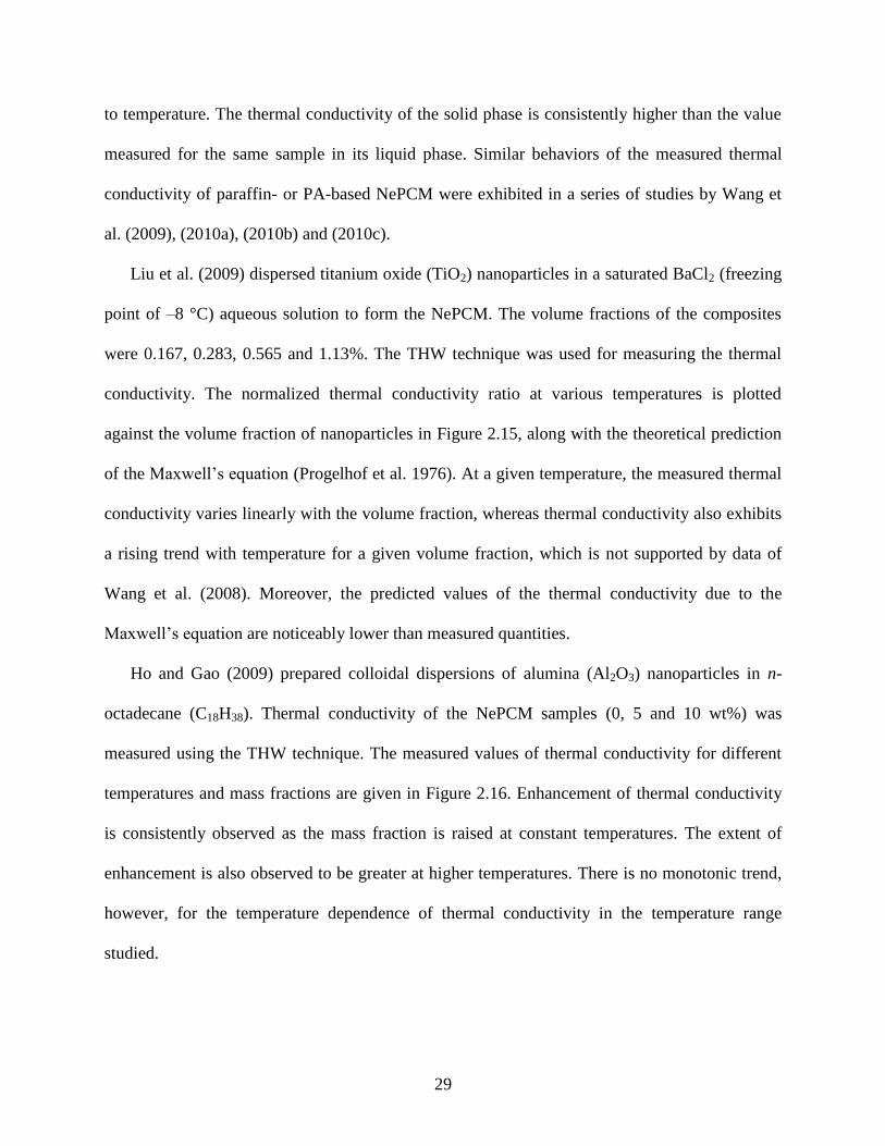
29
to temperature. The thermal conductivity of the solid phase is consistently higher than the value
measured for the same sample in its liquid phase. Similar behaviors of the measured thermal
conductivity of paraffin- or PA-based NePCM were exhibited in a series of studies by Wang et
al. (2009), (2010a), (2010b) and (2010c).
Liu et al. (2009) dispersed titanium oxide (TiO2) nanoparticles in a saturated BaCl2 (freezing
point of –8 °C) aqueous solution to form the NePCM. The volume fractions of the composites
were 0.167, 0.283, 0.565 and 1.13%. The THW technique was used for measuring the thermal
conductivity. The normalized thermal conductivity ratio at various temperatures is plotted
against the volume fraction of nanoparticles in Figure 2.15, along with the theoretical prediction
of the Maxwell’s equation (Progelhof et al. 1976). At a given temperature, the measured thermal
conductivity varies linearly with the volume fraction, whereas thermal conductivity also exhibits
a rising trend with temperature for a given volume fraction, which is not supported by data of
Wang et al. (2008). Moreover, the predicted values of the thermal conductivity due to the
Maxwell’s equation are noticeably lower than measured quantities.
Ho and Gao (2009) prepared colloidal dispersions of alumina (Al2O3) nanoparticles in n-
octadecane (C18H38). Thermal conductivity of the NePCM samples (0, 5 and 10 wt%) was
measured using the THW technique. The measured values of thermal conductivity for different
temperatures and mass fractions are given in Figure 2.16. Enhancement of thermal conductivity
is consistently observed as the mass fraction is raised at constant temperatures. The extent of
enhancement is also observed to be greater at higher temperatures. There is no monotonic trend,
however, for the temperature dependence of thermal conductivity in the temperature range
studied.

30
Zeng et al. (2010) prepared form-stable NePCM composites based on 1-tetradecanol with
various loadings of silver (Ag) nanowires. Thermal conductivity at room temperature was
obtained using the transient planar source (TPS) technique. Two identical cylinder specimens
(diameter of 13 mm) were prepared under higher pressure (20 MPa). The values of the thermal
conductivity of the NePCM samples at room temperature are plotted against the mass fraction of
the Ag nanowires in Figure 2.17. Linear dependence of thermal conductivity over two ranges
(0~40 wt% and 40~70 wt%) is observed. Comparing this property of the form-stable composites
to those of metal powder-filled solid composites, the enhanced thermal conductivity was
attributed to the high aspect ratio of the nanowires.
In addition to the aforementioned efforts devoted to thermal conductivity measurement and
thermal characterization (DSC testing) of NePCM, some of the studies have also investigated the
stability of NePCM upon freeze/thaw cycling and the performance in thermal energy storage
systems. For example, by employing an infrared imaging instrument, the freezing process of
aqueous NePCM with Al2O3 nanoparticles was studied experimentally by Wu et al. (2009). The
0.2 wt% composite exhibited a 20.5% reduced freezing time period.
Later on, the system-level phase change performance of a saturated BaCl2 aqueous solution
enhanced by titanium oxide (TiO2) nanoparticles was tested by Liu et al. (2009) in a cold
storage/supply unit. The enhanced performance of the NePCM that is exhibited by lowering of
the charging/discharging time periods was clearly observed. More recently, Wu et al. (2010)
reported their experimental results of freezing and melting performance of paraffin-based
NePCM. Both the charging and discharging time periods were observed to be shortened by about
30% due to the introduction of 1 wt% copper (Cu) nanoparticles.

31
In addition to the aforementioned experimental efforts, theoretical prediction of enhanced
thermal conductivity of NePCM colloids is also of importance. In the following section, a brief
introduction to the theoretical work on modeling of the effective thermal conductivity of two-
phase mixtures/composites will be presented and the models that are applicable for NePCM
colloids will be discussed.
2.3 Prediction of the Effective Thermal Conductivity of Two-Phase Mixtures
Prediction of the effective transport properties, e.g., thermal conductivity, electrical
conductivity, etc., of two-phase mixtures/composites has been of great interest (Batchelor, 1974).
The essential assumption is that such a heterogeneous media (mixture/composite) consists of a
continuous base material (matrix material) and a discrete phase (particles) dispersed in it
(Progelhof et al., 1976). For the NePCM colloids considered, the base PCM —either in solid or
liquid states— is the continuous phase and the nano-structured thermal conductivity enhancers
constitute as the discrete phase.
The effective thermal conductivity of a two-phase mixture/composite depends on the thermal
conductivity of both constituents, the concentration, dimension, geometry and distribution of the
dispersed particles, and the interfacial effects between the matrix material and particles as well.
In view of the inherent randomness associated with the dispersed particles, microstructures of the
mixtures/composites, i.e., dimension, geometry and distribution of the particles, have often been
excluded in the theoretical work. Therefore, effective thermal conductivity of two-phase
mixtures/composites has mostly been correlated to the thermal conductivities of the matrix
material and particles and concentration (volume fraction) of particles.

32
The simplest model for predicting the effective thermal conductivity of two-phase
mixtures/composites is the mixture rule that takes the following form (Das et al., 2008):
nnn kkkdceff
)1( , (2.1)
where subscripts eff, c and d stand for effective, continuous and discrete phases, and is the
volume fraction of the discrete phase. It is noted that the two extreme cases, i.e., parallel and
series mixture rules, are obtained when the index n takes the values of 1 and –1, respectively.
The predicted values corresponding to these two cases serve as the upper (parallel) and lower
(series) bounds of the predicted effective thermal conductivity. The mixture rule, however, is
only applicable for mixtures/composites with special distributions of particles, e.g., the particles
are packed with a high concentration. For mixtures/composites with dilute concentrations (e.g.,
colloidal suspensions), the applicability of the mixture rule is usually not verified.
For dilute two-phase mixtures/composites with non-interacting spherical particles and in the
absence of thermal interfacial resistance, the effective thermal conductivity can be predicted
using the Maxwell’s equation (Das et al., 2008), as given by
)(2
)(22
dccd
dccd
ceffkkkk
kkkkkk
. (2.2)
This equation was first obtained by Maxwell (1873) for the analogous electrical conductivity
problem of two-phase conductors. Although it is based on very dilute assumption, abundant
experimental data of thermal conductivity of nanofluids have shown that the Maxwell’s equation
is applicable for volume fraction of nanoparticles up to 10 percent (Yu et al., 2008).
As mentioned, the microstructures of particles and interfacial effects are not accounted for in
the Maxwell’s equation. Some extensions based on the Maxwell’s equation have therefore been
explored to address these concerns. For example, Nomura and Chou (1980) presented a

33
theoretical work on the bounds of effective thermal conductivity of composites with short fibers
as the discrete phase. Hasselman and Johnson (1987) and Nan et al. (1997) considered the
interfacial thermal resistance in modeling effective thermal conductivity of particulate
composites. Recently, Evans et al. (2008) further studied the effects of aggregation of
nanoparticles and interfacial thermal resistance on the effective thermal conductivity of
nanocomposites and nanofluids. It should be noted that there are a great number of theoretical
studies available in the literature and only a few representative ones were mentioned above.
The Maxwell’s equation and its extensions are usually classified as ―static‖ models,
indicating that the diffusion of particles, which may contribute to enhancement of heat exchange
between the two phases, is not taken into consideration. This is well-justified if the continuous
phase is stationary (e.g., NePCM in solid state). For colloidal suspensions or structural
composites, the diffusion of particles, however, may play an important role, especially when the
size of the particles is in sub-micron range (e.g., nanofluids). The Brownian motion,
thermophoresis, and osmophoresis of such ultrafine particles have been pointed out to be the
possible mechanisms for thermal conductivity enhancement of nanofluids (Koo and Kleinstreuer,
2005). Although the contribution from diffusion of particles is still controversial, some
―dynamic‖ models for predicting thermal conductivity of nanofluids have been proposed. For
example, Koo and Kleinstreuer (2004) postulated that the effective thermal conductivity of
nanofluids consists of the static and dynamic parts, given by
dynamicstaticeffkkk , (2.3)
where the kstatic is estimated using the Maxwell equation, Eq. (2.2), and the dynamic part kdynamic
is related to the Brownian motion of nanoparticles. It is obvious that the diffusion of

34
nanoparticles is considered to contribute positively to the enhanced thermal conductivity of
nanofluids.
Based on abundant experimental data obtained by over 30 groups worldwide on identical
samples, Buongiorno et al. (2009) found that the measured thermal conductivity of nanofluids
(volume fraction less than 3 percent) was in good agreement of the Maxwell’s equation and the
extended model proposed by Nan et al. (1997) and no anomalous enhancement beyond the static
part was observed. As confidence has been established, the Maxwell’s equation will be used to
predict the effective thermal conductivity of NePCM colloids in the following chapters.
2.4 Summary
A state-of-the-art review of thermal conductivity enhancement of PCM was presented. The
approach to achieve enhanced thermal conductivity was first focused on the use of highly-
conductive fixed structures, e.g., metallic extended surfaces. Emerging advanced materials such
as carbon fibers, graphite and metal foams, were utilized as the conductivity enhancers
depending on the availability of these materials.
The use of nano-materials suspensions as PCM, inspired by the research of nanofluids, has
attracted increasing attention and has become an efficient and promising approach to enhance
thermal conductivity of PCM. In the literature, the nano-additives have included metal and metal
oxide nanoparticles, carbon nanotubes, and nanofibers. The published studies, however, have
mainly focused on preparation and characterization of NePCM and their performance at system
level. There is a lack of mathematical modeling and detailed experimental investigation on
freezing/melting heat transfer of such materials.

35
Finally, a brief introduction of theoretical work on prediction of the effective thermal
conductivity of two-phase mixtures/composites was presented. The origin and applicability of
the well-known Maxwell’s equation for dilute mixtures/composites with non-interacting particles
were discussed. Extensions of the Maxwell’s equation that involve the geometry, interfacial
thermal resistance, and diffusion of particles, etc. were also mentioned.

36
Table 2.1 Summary of the reviewed studies on thermal conductivity enhancement of PCM through fixed structures (Fan and
Khodadadi, 2011)
Authors
(year)
PCM Enhancers Configurations
Study/Measureme
nt Techniques Materials Properties Materials Sizes
Propertie
s
vol% a Types
Bentilla et al.
(1966)
1. tetradecane Tm: 278.8 1. Al wool N/A N/A 10~18% N/A
experiments
2. hexadecane Tm: 289.9 2. Al foam N/A ρ: 900 N/A N/A
3. octadecane Tm: 301.0 3. Cu foam N/A ρ: 500 N/A N/A
4. eicosane Tm: 309.9
4. Al
honeycomb
N/A N/A N/A N/A
Hoover
(1971)
LiNO3-3H2O
Tm: 300
L: 232.4
k: 0.519
Cp: 1.6736 b
ρ: 1,602
1. Al
powder
N/A N/A N/A N/A DSC c
2. Al gauze
3. Al
honeycomb
4. alumina

37
(Al2O3)
foam
5. alumina
powder
Humphries
(1974)
nonadecane Tm: 305.3 Al fins
details
in
paper
N/A N/A
vertically
mounted
1. TCs d
2. visual
observation
Griggs et al.
(1974)
nonadecane N/A Al N/A N/A N/A N/A
transient 2D
numerical study
(diffusion only)
Abhat (1976)
octadecane
(C18H38)
Tm: 301.5
Al
honeycomb
details
in
paper
N/A
~11.5%
(estimate
d by us)
N/A
1. TCs
2. transient non-
equilibrium
numerical study
(diffusion only)
De Jong and 1. pure paraffin Tm: 310 1. Al N/A N/A 10% N/A 1. caloric method

38
Hoogendoorn
(1981)
(n-eicosane
C20H42)
L: 125
k: 0.2 (l) and
~0.10 (s) e
Cp: 2.3 (l) and
2.4 (s)
honeycomb 2. TGA f
3. THW g
4. transient
cylinder
5. TCs
6. enthalpy method
2. commercial
wax
Tm: 315~317
L: ~137
k: 0.19 (l) and
~0.14 (s)
Cp: 2.4 (l) and
2.2 (s)
2. Al thin-
strip matrix
compa
cted as
require
d
N/A
0.4, 0.8
and 1.6%
N/A
Abhat et al.
(1981)
1. eicosane Tm: 310
Al metal
fins
N/A N/A N/A
longitudi
nally
positione
d
1. TCs
2. visual
observation
2. lauric acid Tm: 315~317
3. CaCl2·6H2O Tm: ~303
Henze and octadecane Tm: 301 Al fins flat k: N/A symmetri 1. 2D transient
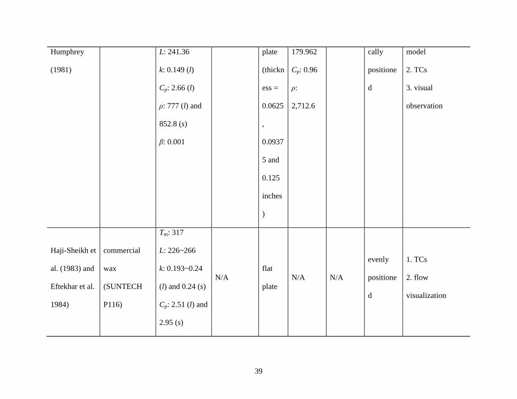
39
Humphrey
(1981)
L: 241.36
k: 0.149 (l)
Cp: 2.66 (l)
ρ: 777 (l) and
852.8 (s)
β: 0.001
plate
(thickn
ess =
0.0625
,
0.0937
5 and
0.125
inches
)
179.962
Cp: 0.96
ρ:
2,712.6
cally
positione
d
model
2. TCs
3. visual
observation
Haji-Sheikh et
al. (1983) and
Eftekhar et al.
1984)
commercial
wax
(SUNTECH
P116)
Tm: 317
L: 226~266
k: 0.193~0.24
(l) and 0.24 (s)
Cp: 2.51 (l) and
2.95 (s)
N/A
flat
plate
N/A N/A
evenly
positione
d
1. TCs
2. flow
visualization

40
ρ: 748~790 (l)
and 818 (s)
β:
0.00204~0.002
16
Knowles and
Webb (1987)
1. hexadecane
k: 0.15
Cp: 2.42
ρ: 760
Al
plate
fins or
wires
k: 240
Cp: 0.926
ρ: 2,700
1, 26 and
50%
uniforml
y
distribute
d
1. transient lumped
model
2. platinum
resistance
thermometer 2. dodecanol
Tm: 295.8
volumetric L:
171 (MJ/m3)
Cu N/A N/A
0, 1.4,
8.9 and
50%
uniforml
y
distribute
d
Chow et al.
(1996)
LiH
Tm: 958
L: 2,580
k: 2.1 (l) and
Ni (S) N/A
k: 92.1
Cp: 0.439
ρ: 8,913
5%
uniforml
y mixed
steady-state
numerical study
(diffusion only)

41
4.2 (s)
Cp: 7.37 (l) and
6.28 (s)
ρ: 550 (l) and
690 (s)
Tong et al.
(1996)
water/ice
k: 0.575 (l) and
2.21 (s)
Cp: 4.217 (l)
and 2.04 (s)
ρ: 999.9 (l) and
917 (s)
Al matrix N/A
k: 237
Cp: 0.896
ρ: 2,707
5, 10 and
15%
uniforml
y
distribute
d
transient numerical
study (convection)
Bugaje (1997) paraffin wax
Tm: 331~333
L: 266
k: 0.24 (l) and
0.24 (s)
Cp: 2.51 (l) and
Al matrix N/A N/A
6 and
20%
N/A TCs

42
2.95 (s)
ρ: 760 (l) and
818 (s)
Pal and Joshi
(1998)
n-triacontane
Tm: 338.6
L: 251
k: 0.23
Cp: 2.05
ρ: 810
Al
honeycomb
side
length:
1.65
mm
height:
14.5
mm
N/A N/A
fully
filled
1. TCs
2. numerical study
(conjugate,
diffusion and
convection)
Velraj et al.
(1999)
paraffins
RT 58 and 60
Tm: 214.4
k: 0.2
Cp: 0.9
ρ: 775 (l) and
850 (s)
1. Al fins N/A
N/A
7 and
20%
internal
longitudi
nal
1. TCs
2. parameter
estimation
3. numerical study
(enthalpy method)
2. lessing
rings
d: 1
cm
randomly
distribute
d 3. water N/A

43
bubbles
Fukai et al.
(1999 and
2000)
paraffin wax
Tm: 314~316
k: 0.26 (s)
carbon
fibers
l: 5,
200
mm
d: 10
μm
k: 220
ρ: 2,170
< 2%
1.
randomly
positione
d
2. fiber
brush
1. TCs
2. parameter
estimation
Cabeza et al.
(2002)
deionized
water
L: 330
k: ~0.6 (l) and
~2.4 (s)
Cp: ~4.1 (l)
ρ: ~1,000 (l)
1. stainless
steel
tube
pieces
l: 25
mm
d: 16
mm
(inner)
, 18
mm
k: 45
Cp:
0.4~0.5
ρ: 7,800
< 10% N/A TCs
2. Cu
k: 393
Cp: 0.383
ρ: 8,900

44
(outer)
3. graphite
matrix
N/A
k:
25~470
cp: 1.4
ρ: 2,300
Ettouney et al.
(2004)
paraffin wax
Tm: 325
L: 210
k: ~0.15 (l) and
~0.24 (s)
Cp: ~2.1 (l) and
~2.9 (s)
ρ: ~860 (l) and
~780 (s)
1. stainless
steel screens
l: 0.32
m
w:
0.02 m k: 40
Cp: 0.5
ρ: 7,801
0.1~3.4%
radially
positione
d
TCs
2. stainless
steel spheres
d: 8,
12,
and 16
mm
attached
to metal
screens
Stritih (2004) paraffin RT 30 Tm: ~306 steel fins
0.5 m
(h) ×
0.12 m
k: 20 ~5%
fins
evenly
spaced
TCs

45
(l) × 1
mm
(thickn
ess)
Koizumi
(2004)
n-octadecane
Tm: 301
L: 244
k: 0.15 (l) and
0.21 (s)
ρ: 733 (l) and
890 (s)
Cu plates N/A N/A N/A
cross-
shaped
fins
1. TCs
2. flow
visualization
Mesalhy et al.
(2005)
generic PCM
Tm: 300.4
k(s)/k(l) =
2.419
Cp(s)/Cp(l) =
0.964
Pr: 46.1
high
conductivity
solid matrix
N/A
k(matrix)
/
k(PCM)
= 50, 100
and 200
5, 10 and
15%
rectangul
ar cells
with
conductiv
e fibers
thermal non-
equilibrium
numerical study

46
Ettouney et al.
(2006)
paraffin wax
Tm: 325
L: 210
k: 0.15 (l) and
0.24 (s)
Cp: 2.1 (l) and
2.9 (s)
ρ: 780 (l) and
860 (s)
stainless
steel spheres
d: 4, 5
and 6
mm
k: 20
Cp: 0.46
ρ: 7,846
N/A
accumula
ted on the
bottom
TCs
Nayak et al.
(2006)
eicosane
Tm: 310
L: 241
k: 0.157 (l) and
0.39 (s)
Cp: 2.2 (l) and
1.9 (s)
ρ: 770 (l) and
810 (s)
1. Al matrix
d =
420
μm k: 179.6
Cp: 0.96
ρ:
2,712.9
5, 10 and
15%
uniforml
y filled
with
PCM transient numerical
study (diffusion
and convection)
2. Al fins N/A
10, 20
and 30%
1. plate-
type
2. rod-
type
47
Nakaso et al.
(2008)
paraffin wax
Tm: 322.2
k: 0.12 (l) and
0.21 (s)
ρ: 780 (l) and
900 (s)
Woven
carbon fiber
sheets and
carbon fiber
brushes
10 μm
in
diamet
er
fibers
k: 190
Cp: 1
ρ: 2,120
0.21 and
0.42 for
sheets,
0.75 for
brushes
1. cloth
wrapping
copper
tubes
2. fiber
brushes
1. inlet/outlet
temperature
measurements
2. transient
modeling of
conduction
Agyenim et
al. (2009)
erythritol
(C4H10O4)
Tm: 390.9
L: 339.8
k: 0.326 (l) and
0.733 (s)
Cp: 2.76 (l) and
1.38 (s)
ρ: 1,300 (l) and
1,480 (s)
Cu plates
used as
circular and
longitudinal
fins
1 mm
(thickn
ess)
N/A
Not given
but can
be
computed
radial and
longitudi
nal fins
1. DSC
2. TCs
a vol% denotes the volume fraction.
b The unit for the specific heat Cp is kJ/kgK.

48
c DSC denotes the differential scanning calorimetry.
d TCs stands for thermocouples.
e l in parentheses indicates the liquid phase, and s for the solid.
f TGA denotes thermal gravimetric analysis.
g THW denotes transient hot wire method.

49
Table 2.2 Summary of the configurations of experimental setups and thermal operating conditions of the reviewed studies (Fan
and Khodadadi, 2011)
Authors (year) Geometries
Insulated
Surfaces
Volumes a
Phase
Change
Types
Heating/Cooling Schemes
Thermal
Conditions
Gravity/Heat
Fluxes Angle
b
Abhat (1976)
rectangular
box
5 c 2,166 melting
H d: CHF
e MINCO heater
foil
0.03 to 0.325
W/cm2
180°
De Jong and
Hoogendoorn
(1981)
cylindrical
tube
T B f 347
freezing
T: outer water stream 10 to 20 °C below
melting temp.
90°
annular tube S 377
T: inner tube heat
exchanger
somewhat below
melting temp.
90°
Abhat et al.
(1981)
annular tube T B 750
melting
T: CT at one end of heat
pipe
kept at 50 °C
0° ~ 180°
freezing T: CT outer liquid flow kept at 15 °C
Henze and
Humphrey
rectangular
box
3 103 melting T: CT MINCO heater foil kept at 5, 10, 15
and 20 °C above
90°

50
(1981) melting temp.
Eftekhar et al.
(1984)
rectangular
box
4 55.4 melting T: CT hot and cold plates
kept the top (cold)
and bottom (hot)
walls at various
temp. gradients
180°
Knowles and
Webb (1987)
cylindrical
tube
T S 393 melting
H: CHF copper heater
plate
kept at 12.7
kW/m2
180°
Bugaje (1997)
cylindrical
tube
T B 270
melting
T: outer air flow
69 to 81 °C 90°
freezing 25 to 45 °C 90°
Pal and Joshi
(1998)
rectangular
box
5 292.4 melting
H: CHF silicone rubber
patch heater
increased from 15
to 60 W at a step
of 5 W
180°
Velraj et al.
(1999)
cylindrical
tube
N/A 1,374 freezing T: CT water bath kept at 50, 54 and
55 °C
90°
Fukai, et al.
(1999 and
cylindrical
tube
T B 255
melting
T: CT water bath 20 to 60 °C 90°
freezing

51
2000)
Cabeza et al.
(2002)
rectangular
box
5 4,647
melting T: CT planar heat
exchanger
kept at 15 °C 90°
freezing kept at –15 °C 90°
Ettouney et al.
(2004)
annular tube S 1,534 melting
T: inner tube heat
exchanger
various inlet
temps. with
constant flow rate
90°
Stritih (2004)
rectangular
box
5 39,000
melting
T: planar heat exchanger
65 °C inlet temp. 90°
freezing 18 °C inlet temp. 90°
Koizumi
(2004)
spherical
container
N/A 58 melting T: outer air flow 20 °C above
melting temp.
180°
Ettouney et al.
(2006)
spherical
container
N/A 11.5 melting T: outer air flow 70, 80 and 90 °C
inlet temp.
180°
Agyenim et
al. (2009)
annular tube N/A 14,500
melting
T: heat exchange with
silicone oil
140 °C inlet temp.
90°
freezing
T: heat exchange with
water
70 °C inlet temp.
52
a This column gives the total volume occupied by both PCM and promoters (unit: cc).
b This column provides the angle between the gravitational acceleration vector and heat fluxes.
c The number in this column specifies how many surfaces are insulated when a rectangular box is being investigated.
d H means the heat flux input is known and T means the surface temperature is known.
e CHF denotes constant heat flux, and CT denotes constant temperature.
f T, B and S stand for the top, bottom and side walls of a cylindrical or annular tube, respectively.

53
Table 2.3 Summary of the base PCM and nano-structured materials considered in the published NePCM articles
Authors (year)
PCM Nano-structured materials
Materials Properties Materials Properties Sizes Fractions
Elgafy and Lafdi
(2005)
paraffin wax
Tm: ~67 °C
k: ~0.24 W/mK
: 1.51 × 10⁻⁷
m2/s
carbon nanofibers (CNF)
: ~1,600
kg/m3
outer diameter:
~100 nm, length:
~20 m
1, 2, 3 and 4 wt%
a
Khodadadi and
Hosseinizadeh
(2007)
water
: 997.1 kg/m3
Cp: 4,179 J/kgK
k: 0.6 W/mK
: 8.9 × 10⁻⁴
kg/ms
β: 2.1 × 10⁻⁴
1/K
L: ~335,000 J/kg
copper (Cu) nanoparticles
: 8,954 kg/m3
Cp: 383 J/kgK
k: 400 W/mK
β: 1.67 × 10⁻⁵
1/K
10 nm 10 and 20 vol%
Zeng et al.
(2007)
1-tetradecanol
(C14H30O)
Tm: ~38 °C
L: ~230,000 J/kg
silver (Ag) nanoparticles N/A 500 nm 2~94 wt%

54
Zeng et al.
(2008)
C14H30O and
C14H30O/PANI b
Tm: ~35 °C
L: 221,250 and
119,140 J/kg
multi-walled carbon
nanotubes (MWCNT)
N/A
outer diameter:
10~30 nm, length:
5~15 m
0.5, 1, 2.5 and 5
wt%
Shaikh et al.
(2008)
paraffin wax
(shell wax 100)
L: 156,300 J/kg
single wall carbon
nanotubes (SWCNT),
MWCNT, and CNF
N/A
diameter: 1, 10 and
100 nm
0.1, 0.4, 0.7 and 1
vol%
Wang et al.
(2008)
palmitic acid
(PA), purity
98%
Tm: 62.5~64 °C
: 853 kg/m3
k: 0.24 W/mK
L: 207,800 J/kg
MWCNT, surface-
oxidized by a mixed acid
with 1:3 of concentrated
nitric and sulfuric acids
N/A
diameter: 30 nm,
length: 50 m,
specific surface
area: 60 m2/g
0.5, 1, 2 and 5
wt%
Zeng et al.
(2009)
PA
Tm: 59.48 °C
Tf: 58.78 °C
k: 0.318 W/mK
L: ~201,000 J/kg
pristine MWCNT,
surface-oxidized
MWCNT (by two acids)
N/A
outer diameter:
10~30 nm, length:
5~15 m (long),
1~2 m (short)
0.0999~4.762
wt% (without
surfactants), and
0.095~4.55 wt%
(with surfactants)
Liu et al. (2009) saturated barium Tf: –8 °C titanium oxide (TiO2) N/A 20 nm 0.167, 0.283,

55
chloride (BaCl2)
aqueous
solution
pH: 8 nanoparticles 0.565 and 1.13
vol%
Wu et al. (2009) distilled water k: 0.6008 W/mK
alumina (Al2O3)
nanoparticles
N/A 20 nm
0.05, 0.1 and 0.2
wt%
Ho and Gao
(2009)
n-octadecane
(C18H38)
Tm: 26.5 °C
Tf: 25.1 °C
L: ~243,100 J/kg
Al2O3 nanoparticles : 3,600 kg/m3
33 nm (159.6 and
196.0 nm in
suspensions)
5 and 10 wt%
Wang et al.
(2009)
paraffin wax
Tm: 53 °C
L: ~165,300 J/kg
MWCNT, treated by ball
milling
N/A
diameter: 30 nm,
length: 50 m,
specific surface
area: 60 m2/g
0.2, 0.5, 1.0 and
2.0 wt%
Zeng et al.
(2010)
C14H30O
k: 0.32 W/mK
L: ~220,000 J/kg
Ag nanowires N/A N/A 9.09~62.73 wt%
Wang et al.
(2010a)
paraffin wax
Tm: ~48.1 °C
L: 142,200 J/kg
γ- Al2O3 nanoparticles : 3,900 kg/m3 20 nm 1, 2 and 5 wt%

56
Wang et al.
(2010b)
PA, purity 98%
Tm: 62.4 °C
k: 0.22 W/mK
(solid)
k: 0.16 W/mK
(liquid)
L: 208,000 J/kg
MWCNT, treated by
mechano-chemical
reaction with potassium
hydroxide
N/A
diameter: 30 nm,
length: 50 m,
specific surface
area: 60 m2/g
0.2, 0.5 and 1.0
wt%
Wang et al.
(2010c)
PA, purity 98%
Tm: 62.5~64 °C
k: 0.223 W/mK
(solid)
k: 0.154 W/mK
(liquid)
MWCNT, treated by
various methods,
including surface
oxidation, mechano-
chemical reaction, ball
milling, and grafting
following acid oxidation
N/A
diameter: 30 nm,
length: 50 m,
specific surface
area: 60 m2/g
0.2, 0.5 and 1.0
wt%
Wang et al.
(2010d)
paraffin wax,
purity 99.99%
Tm: 58~60 °C Cu nanoparticles N/A
diameter: 25 nm,
specific surface
area: 30~50 m2/g,
0.1, 0.5, 1 and 2
wt%

57
purity: 99.9%
Wu et al. (2010) paraffin Tm: 58~60 °C
Cu, Al and C/Cu
nanoparticles
N/A
diameter: 25 nm,
purity: 99.9%
0.1 wt% for all
three kinds of
nanoparticles, 0.1,
0.5, 1 and 2 for
Cu nanoparticles
Cui et al. (2011)
paraffin and soy
wax
Tm: 52~54 °C CNF, MWCNT N/A
outer diameter:
200 nm (CNF)
diameter: 30 nm,
length: 50 m,
specific surface
area: 60 m2/g,
purity: 95% (CNT)
1, 2, 5 and 10
wt%
a vol% and wt% stand for volumetric and mass fractions, respectively.
b PANI denotes polyaniline.

58
Table 2.4 Summary of preparation and characterization methods and instruments in the published NePCM articles
Authors (year)
Preparation Characterization
Studies of heat transfer
Methods
Dispersion and
stabilization a
Thermal
conductivity
Other measurements
and instruments
Stability
Elgafy and Lafdi
(2005)
two-step
shear mixing (in
liquid state)
calculated using
measured and
Cp
DSC b and laser
flash technique
N/A
TC readings for a
thaw/freeze test,
analytic model for
predicting thermal
conductivity
Khodadadi and
Hosseinizadeh
(2007)
N/A N/A
Maxwell’s
equation
N/A N/A CFD modeling
Zeng et al. (2007) one-step N/A N/A
DSC, FTIR c, TEM,
TGA and XRD
N/A TC readings
Zeng et al. (2008) two-step sonication
Hot Disk thermal
constants
DSC, SEM e and
TGA
N/A N/A
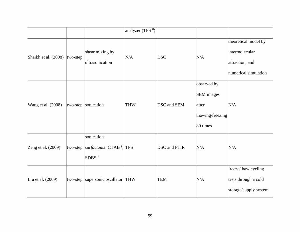
59
analyzer (TPS d)
Shaikh et al. (2008) two-step
shear mixing by
ultrasonication
N/A DSC N/A
theoretical model by
intermolecular
attraction, and
numerical simulation
Wang et al. (2008) two-step sonication THW f DSC and SEM
observed by
SEM images
after
thawing/freezing
80 times
N/A
Zeng et al. (2009) two-step
sonication
surfactants: CTAB g,
SDBS h
TPS DSC and FTIR N/A N/A
Liu et al. (2009) two-step supersonic oscillator THW TEM N/A
freeze/thaw cycling
tests through a cold
storage/supply system
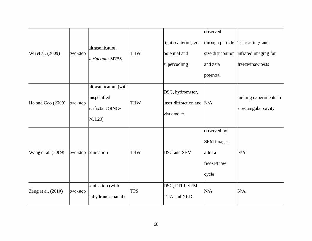
60
Wu et al. (2009) two-step
ultrasonication
surfactant: SDBS
THW
light scattering, zeta
potential and
supercooling
observed
through particle
size distribution
and zeta
potential
TC readings and
infrared imaging for
freeze/thaw tests
Ho and Gao (2009) two-step
ultrasonication (with
unspecified
surfactant SINO-
POL20)
THW
DSC, hydrometer,
laser diffraction and
viscometer
N/A
melting experiments in
a rectangular cavity
Wang et al. (2009) two-step sonication THW DSC and SEM
observed by
SEM images
after a
freeze/thaw
cycle
N/A
Zeng et al. (2010) two-step
sonication (with
anhydrous ethanol)
TPS
DSC, FTIR, SEM,
TGA and XRD
N/A N/A

61
Wang et al. (2010a) two-step
sonication (with
oleylamine)
THW
DSC, FTIR, SEM,
TEM and XRD
N/A N/A
Wang et al. (2010b) two-step sonication THW
DSC, FTIR and
SEM
N/A N/A
Wang et al. (2010c) two-step sonication THW
FTIR, SEM, TEM
and XRD
N/A N/A
Wang et al. (2010d) two-step
ultrasonication
surfactant: gum
Arabic
N/A DSC and TEM
visually
observed
TC readings for a
thaw/freeze test
Wu et al. (2010) two-step
ultrasonication
surfactants: gum
Arabic, Span-80,
CTAB, SDBS and
Hitenol BC-10
N/A DSC and FTIR
visually
observed,
thermal stability
test for up to 100
cycles by DSC
TC readings for a
thaw/freeze test
Cui et al. (2011) two-setp ultrasonication THW DSC and SEM N/A
TC readings for heating
tests

62
a This column is only applicable to the two-step method.
b DSC stands for differential scanning calorimetry.
c FTIR, TEM, TGA and XRD stand for Fourier transform infrared spectroscopy, transmission electron microscopy, thermal
gravimetric analysis and X-ray diffraction, respectively.
d TPS denotes transient plane source technique.
e SEM denotes scanning electron microscope.
f THW stands for transient hot wire method.
g CTAB denotes cetyltrimethyl ammonium bromide.
h SDBS denotes sodium dodecylbenzene sulfonate.
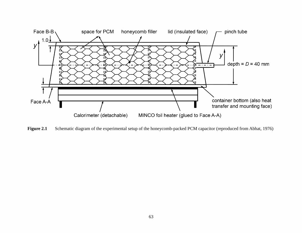
63
Figure 2.1 Schematic diagram of the experimental setup of the honeycomb-packed PCM capacitor (reproduced from Abhat, 1976)

64
Figure 2.2 Schematic diagram of the visualized double-finned rectangular test cell for
melting of PCM (Henze and Humphrey, 1981)

65
Figure 2.3 Comparison of the progress of melting between the experimental results (left column) by Henze and Humphrey (1981)
and numerical predictions (right column)

66
Figure 2.4 Comparison of the freezing times for different designs of the aluminum matrices
at various boundary temperatures (Bugaje, 1997)
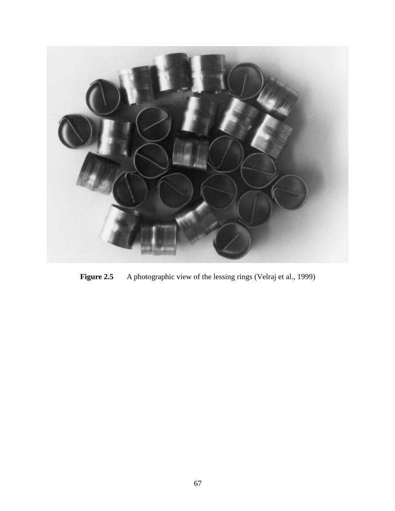
67
Figure 2.5 A photographic view of the lessing rings (Velraj et al., 1999)

68
Figure 2.6 Thermal conductivity enhancement of PCM as a function of volume fraction of
the inserted carbon fibers (Fukai et al., 2000)

69
Figure 2.7 Schematic diagram of the cross-sectional view of the cylindrical PCM container
showing locations of the metal screens with mounted metal spheres and thermocouples (Ettouney
et al., 2004)

70
Figure 2.8 The absorbed heat as a function of Fourier number for (a) different porosities of
the matrix and (b) different matrix to PCM conductivity ratios (Mesalhy et al., 2005)

71
Figure 2.9 Arrangements and dimensions (in mm) for three kinds of PCM/enhancer
combinations: (a) matrix, (b) plate-type fins, (c) front and (d) top views of rod-type fins (Nayak
et al., 2006)

72
Figure 2.10 Comparison of the instantaneous melting fractions among the three types of
enhancers (Nayak et al., 2006)

73
Figure 2.11 Schematic diagrams of the two installation options of carbon fibers: (a) cloths and
(b) brushes (Nakaso et al., 2008)
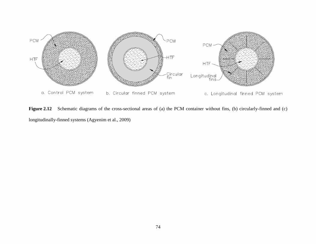
74
Figure 2.12 Schematic diagrams of the cross-sectional areas of (a) the PCM container without fins, (b) circularly-finned and (c)
longitudinally-finned systems (Agyenim et al., 2009)
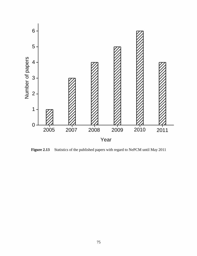
75
1 2 3 4 5 60
1
2
3
4
5
6
20112010200920082007
Nu
mb
er
of
pap
ers
Year
2005
Figure 2.13 Statistics of the published papers with regard to NePCM until May 2011

76
Figure 2.14 Measured temperature-dependent thermal conductivity of PA-based NePCM
samples with MWCNT at various mass fractions (Wang et al., 2008)

77
Figure 2.15 Measured thermal conductivity of BaCl2 aqueous solutions enhanced by various
volume fractions of TiO2 nanoparticles (Liu et al., 2009)

78
Figure 2.16 Measured temperature-dependent thermal conductivity of octadecane-based
NePCM samples with Al2O3 nanoparticles (Ho and Gao, 2009)

79
Figure 2.17 Measured thermal conductivity of 1-tetradecanol-based NePCM samples with Ag
nanowires at various mass fractions (Zeng et al., 2010)

80
Chapter 3 Preparation of NePCM Colloids and Measurement of Their Thermal Conductivity
In this chapter, investigation on thermal conductivity enhancement of NePCM colloids is
discussed. Preparation procedures of cyclohexane- and eicosane-based NePCM samples with
copper oxide nanoparticles are presented, followed by a brief introduction of the TPS technique
and instrument. The measured thermal conductivity of NePCM samples, in both liquid and solid
phases, is then presented as a function of temperature and the loading of nanoparticles.
Uncertainties and difficulties associated with the solid phase experiments are highlighted.
3.1 Preparation of Hydrocarbon-Based NePCM Colloids
3.1.1 Selection of base PCM and concern of colloidal stability
The proper candidates of PCM for a particular application are usually chosen based on their
melting/freezing temperatures in relation to the desired temperature range of the application. For
example, alkanes with high carbon numbers (i.e., paraffin wax) have widely been used for the
intermediate temperature range (0~100 °C). When it comes to high temperature applications (>
300 °C), molten salts have long been considered the favored candidates. Therefore, the extension
of potential utility of nanofluids as NePCM will draw attention to base liquids (PCM) other than
water and ethylene glycol. Unfortunately, there is usually a lack of thermophysical properties of
PCM in solid phase, although such data are sometimes well-documented for liquid PCM, e.g.,
water- and ethylene-glycol-based nanofluids (Yu et al. 2008). The knowledge of accurate

81
thermal conductivity data in both phases, however, is also demanded by the analytic and
numerical studies of phase change heat transfer of NePCM.
In the present study, two hydrocarbons with different carbon numbers are chosen as the base
PCM, i.e., cyclohexane (C6H12) and eicosane (C20H42). Cyclohexane is a cycloalkane used as a
non-polar solvent in the chemical industry and possesses a freezing point of 6.5 °C and is
transparent in both phases. Therefore, it has been preferred in visualized freezing experiments
(e.g., Sulfredge et al. 1993). Eicosane that is an alkane with a melting point of about 37 °C is a
white wax-like solid at room temperature and has been widely used as the PCM in studies of
melting. Another alkane, i.e., octadecane (C18H38), has also appeared as PCM candidate in
thermal comfort applications because it has a melting point around 28 °C. The molecular
structures of both selected PCM are illustrated in Figure 3.1 (available at:
http://upload.wikimedia.org/wikipedia/commons/thumb/c/c6/Cyclohexane-chair-3D-balls.png/
100px-Cyclohexane-chair-3D-balls.png, and http://upload.wikimedia.org/wikipedia/commons/
thumb/d/d7/Icosane-3D-balls.png/800px-Icosane-3D-balls.png). The density, latent heat of
fusion and melting/freezing temperatures of the two selected base PCM in their liquid phase are
presented in Table 3.1.
Nanofluids with suspended sub-micron ultra-fine particles (nanoparticles) belong to the
category of colloids (colloidal suspensions). The use of colloids as engineered nanofluids has
added a new dimension of research of colloid chemistry. The instability of particles is the key
challenge for the utilization of nanofluids, especially when the suspensions are used as NePCM
subjected to repeated melting/freezing cycles. The mechanisms of particle aggregation and
precipitation in colloids have been discussed in detail by Heimenz and Rajagopalan (1997) and
the stabilization methods have long been sought. As pointed out by Clary and Mills (2011),

82
electrostatic and steric methods have widely been accepted as two primary modes of kinetic
strategy to improve colloidal stability. The electrostatic stabilization takes advantage of the
repulsion of electrical double layers surrounding the particles, i.e., the Coulombic effect, whereas
the steric approach is achieved by coating ligands to the particle surfaces to protect the particles
from agglomerating together (Clary and Mills, 2011). An idealized model of such ―cushion‖
effect is schematically shown in Figure 3.2. In this manner, polymers are commonly used as
surfactants to stabilize metal and metal oxide nanoparticles.
3.1.2 Preparation of hydrocarbon-based NePCM with stabilized CuO nanoparticles
In the present study, the copper (II) oxide (CuO) nanoparticles stabilized by capping with
sodium oleate acid (SOA, C18H33NaO2) were synthesized and provided by colleagues in the
Department of Chemistry and Biochemistry (Clary and Mills, 2011). A TEM image clearly
exhibits that, as shown in Figure 3.3, the CuO nanoparticles were nearly spherical, and that most
of them possess a diameter within the range of 5 to 15 nm. It is noted that the TEM image was
taken after the nanoparticles were prepared and further processed for the TEM procedure. It is
well-known that such processing leads to agglomeration of the particles due to van del Waals
forces and that is what is being observed in Figure 3.3. In effect, the TEM image does not
represent the actual particle size and distribution within the suspensions. Due to agglomeration
upon forming the suspensions, the actual size of the nanoparticles are expected to grow to some
extent.
Desirable long-term stability of colloidal suspensions containing these sodium-oleate-
stabilized CuO nanoparticles in various hydrocarbons (hexane, octane, dodecane and eicosane)
was observed both qualitatively and quantitatively for mass fraction up to 20 wt%, corresponding

83
to volume fraction of about 3.0 vol% (Clary and Mills, 2011). In the present study, more dilute
NePCM samples were considered and hence, their stability was expected to be acceptable.
Nearly homogeneous NePCM samples were prepared by dispersing the desired amounts of
CuO nanoparticles into the base PCM, i.e., a 99.96% cyclohexane (Pharmco-Aaper, Brookfield,
CT) and a 99% eicosane (Sigma-Aldrich, St. Louis, MO), in liquid phase, then heating and
stirring rigorously at 60 °C (for cyclohexane) or 80 °C (for eicosane) on a hot-plate magnetic
stirrer (SP131325Q, Thermo Fisher, Dubuque, IA) for 30 minutes. Due to the introduction of
CuO nanoparticles, ink-like NePCM samples were obtained. As an example, the eicosane-based
NePCM samples with various mass fractions (0, 1, 2, 5 and 10 wt%) are shown in Figure 3.4.
Although it is seen that more nanoparticles tended to stick on the walls with increasing particle
loading, no significant precipitation was visually found at the bottom of the containers, even for
the most concentrated 10 wt% sample. Cyclohexane-based NePCM samples were prepared for
four (4) mass fractions (0, 1, 2 and 4 wt%). The NePCM samples were stored in a freezer prior to
the measurements.
It should be noted that while calculating the required amounts of nanoparticles for the given
mass (or volume) fractions, the presence of surfactant (SOA in this case) was neglected and the
nanoparticles were considered as pure CuO. Moreover, due to the lack of actual density value of
the nanoparticles, density of bulk CuO (6,315 kg/m3, available at http://www.sciencelab.com/
xMSDS-Cupric_oxide-9923595) was used in the calculations. The samples were prepared with
given mass fractions. In case the corresponding volume fractions are of interest, however, the
following relations were used to fulfill the mass/volume fraction conversion (vol to wt, or vice
versa) for a two-component system:
NPwtPCMwt
PCMwt
vol)1(
, (3.1)
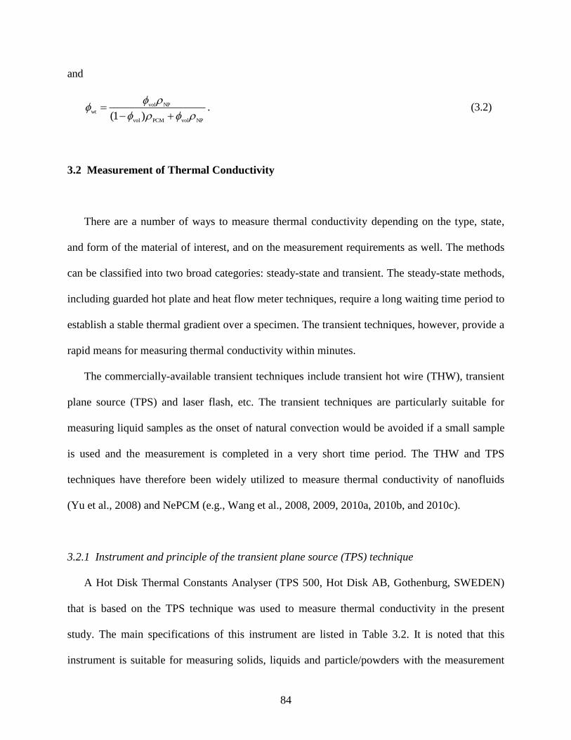
84
and
NPvolPCMvol
NPvol
wt)1(
. (3.2)
3.2 Measurement of Thermal Conductivity
There are a number of ways to measure thermal conductivity depending on the type, state,
and form of the material of interest, and on the measurement requirements as well. The methods
can be classified into two broad categories: steady-state and transient. The steady-state methods,
including guarded hot plate and heat flow meter techniques, require a long waiting time period to
establish a stable thermal gradient over a specimen. The transient techniques, however, provide a
rapid means for measuring thermal conductivity within minutes.
The commercially-available transient techniques include transient hot wire (THW), transient
plane source (TPS) and laser flash, etc. The transient techniques are particularly suitable for
measuring liquid samples as the onset of natural convection would be avoided if a small sample
is used and the measurement is completed in a very short time period. The THW and TPS
techniques have therefore been widely utilized to measure thermal conductivity of nanofluids
(Yu et al., 2008) and NePCM (e.g., Wang et al., 2008, 2009, 2010a, 2010b, and 2010c).
3.2.1 Instrument and principle of the transient plane source (TPS) technique
A Hot Disk Thermal Constants Analyser (TPS 500, Hot Disk AB, Gothenburg, SWEDEN)
that is based on the TPS technique was used to measure thermal conductivity in the present
study. The main specifications of this instrument are listed in Table 3.2. It is noted that this
instrument is suitable for measuring solids, liquids and particle/powders with the measurement

85
time being as short as 2.5 seconds. The thermal conductivity of hydrocarbon-based NePCM was
expected to be of the order of 0.1 W/mK, which lies in the range specified by the manufacturer.
The principle of operation and data reduction of the TPS technique have been presented in
detail by Gustafsson (1991) and Gustavsson et al. (1994), and in the ISO Standard (ISO 22007-
2:2008) as well. A brief introduction to the theory of TPS is presented below. As schematically
shown in Figure 3.5, a double-spiral-shaped hot disk with an outer nominal radius r is used as the
planar heat source (http://www.thermal-instruments.co.uk/Images/sensor1.gif). The sensor is made
of a 10 m thick nickel (Ni) strip. In addition to serving as a heat source to increase the
temperature of the specimen, this sensor also acts as a resistance thermometer for recording the
transient temperature rise. Both sides of the sensor are coated with thin layers of polyimide
(Kapton) as the support material. The Kapton layers allow the sensor to be resistant against most
of the common chemicals, and to work in the temperature range from 10 to 500 K. During the
measurements, the TPS sensor needs to be sandwiched between two identical samples (solids), or
submerged in the sample (liquids), as required by the theory.
The fundamental assumption of the TPS theory is that the sensor consists of a number of
concentric ring heat sources in an infinitely large sample. Therefore, the thermal penetration depth
of the ―thermal wave‖ from the sensor must not reach the physical boundaries of the sample during
the measurements. As given in the instruction manual (ThermTest Inc., Fredericton, New
Brunswick, CANADA), the thermal penetration depth (d) can be estimated by
td 2 , (3.3)
where is the thermal diffusivity of the sample being measured and t is the measurement time.
When the sensor is electronically heated, the transient increase of the resistance R(t) is given by
)]}([1{)(avgK0 TTRtR , (3.4)

86
where R0 is the initial resistance at t = 0, the temperature coefficient of resistance (TCR), TK the
constant temperature difference over the two sides of a Kapton layer, and Tavg() the average
temperature rise of the sample surface on the internal side of the Kapton layers.
Manipulation of the above equation leads to
1
)(1)(
0
avgKR
tRTT
, (3.5)
which represents the temperature increase recorded by the sensor.
As mentioned before, TK can be considered as a measure of the thermal contact resistance
between the sensor and the sample surface. The value of TK vanishes if a perfect thermal contact is
achieved. In real-world measurements, TK will become constant after a very short time period tK
that may be estimated as
K
2
K
K
t , (3.6)
where K and K are the thickness of the Kapton layers and the thermal diffusivity of the Kapton
material, respectively.
Moreover, the average temperature rise is related to thermal conductivity k of the sample as
)(π
)(2/3avg
Drk
PT , (3.7)
where P is the total output of power applied by the sensor, r the outer radius of the sensor, and D()
a dimensionless time-dependent function. The dimensionless time is defined as
2r
t , (3.8)
where time t is the measurement time period, and stands for the thermal diffusivity of the sample.

87
Based on Eq. (3.7), a linear curve fitting for Tavg() as a function of D() allows determination
of both TK (intercept) and P/3/2
rk (slope). Several recorded data points at the very beginning must
be excluded so as to discard the noisy information during the period of tK. Since the power is
prescribed and the radius of the sensor is also a known design parameter, thermal conductivity of
the sample is readily obtained.
As recommended by the instruction manual, the relaxation time between repeated
measurements would be greater than 36 times the time duration of the measurement. For example, if
the measurement time is 5 second, the waiting time between two consecutive measurements would
be longer than 3 minutes. It is noted that thermal diffusivity of the sample is a byproduct during the
measurement process. However, thermal diffusivity of NeCPM samples that is of less interest will
not be presented below.
3.2.2 Experimental setup and procedure
A programmable temperature bath/circulator (TC-502P, Brookfield, Middleboro, MA) with an
stability of 0.01 °C was used to control the measurement temperature. A cylindrical aluminum (Al)
block (diameter of 76.2 mm and height of 127.0 mm) with four holes (diameter of 25.3 mm and
height of 14.0 mm) drilled on the top end was designed and fabricated. The Al block, which was
placed within the reservoir of the constant-temperature bath, served as an isothermal sample holder
because of its much higher thermal diffusivity ( = 84.18 mm2/s, available at
http://en.wikipedia.org/wiki/Thermal_diffusivity) compared to the bath fluids (e.g., water, = 0.14
mm2/s). Cylindrical glass (Pyrex) containers (outer diameter of 25.0 mm and height of 19.0 mm)
that fit the holes were also fabricated. For ease of cleaning and refilling, the measurements were

88
performed with NePCM samples in the glass containers that were placed on one end of the Al
holder.
The TPS sensor being used in the present study was No. 5465 which has an outer radius of the
double-spiral heater of 3.189 mm. The TPS sensor was suspended vertically in the middle of a glass
container, as shown in Figure 3.6. It should be noted that the tip of the sensor (i.e., the double-spiral
heater) must be completely submerged in the sample. Based on the size of the sensor, the minimum
sample volume required was approximately 6 mL for such cylindrical containers. This small size of
the sample volume was favorable for measuring liquid samples, because the incurred undesirable
natural convection during measurements would be suppressed. It was assured in all the
measurements that the estimated thermal penetration depth (d) given by Eq. (3.3) was greatly
smaller than the distances of the sensor to the walls of the sample holder.
At each measurement temperature of interest, thermal equilibrium in the samples was assured
by waiting for 30 minutes after the bath temperature had reached the set point, even though the low
thermal resistance of the Al holder offers a very short response time to the change of bath
temperature. In addition to the internal temperature sensor of the bath, an external 2-wire thermistor
(A733F-CSP60BT103M, GE Sensing, St. Marys, PA) was also used to monitor the bath
temperature. The thin gap between the glass container and the Al holder was filled with the bath
fluid (water/ethylene glycol 1:1 mixture) to lower the contact resistance. In addition, during the
measurements, a lid made of laminated cardboard was used to cover the opening of the glass
container (not shown in Figure 3.6), in an effort to reduce the convective and radiative heat
losses/gains to/from the environment.
The phase of the samples during measurements was controlled by specifying the
measurement temperature. The samples were poured into the glass containers in their liquid

89
phases. The measurements were first performed for samples in their liquid phase. Then the bath
temperature was set to be below the freezing/melting points of the samples so as to have
frozen/solidified samples. By utilizing this solidification scheme, no special effort was needed to
make distinct arrangements for measuring samples in solid and liquid phases.
Finally, after performing the measurements, the TPS sensor and container were cleaned up
using acetone (C3H6O), which is widely used as the solvent for cleaning purposes in the
laboratory. As advised by the manufacturer, cleaning of the TPS sensor should be performed
carefully and quickly, in order to avoid any damage on the embedded thin nickel structures and
the Kapton coating surfaces.
3.2.3 Verification of accuracy and reproducibility of the TPS instrument
Prior to performing measurements for NePCM samples, the accuracy and reproducibility of the
Hot Disk Thermal Constants Analyser were tested. Two individual tests at different times, each of
which had ten (10) runs, were performed with common purified water at room temperature (21 1
°C) and atmospheric pressure (0.1 MPa abs).
As listed in Table 3.3, the average thermal conductivities of both tests were found to be 0.5971
W/mK ± 0.364% and 0.6012 W/mK ± 0.500%. These two values are consistent with each other,
and are in excellent agreement with the well-established quantity of 0.6009 W/mK (Ramires et al.
1995) for water at room temperature (21.85 °C) and atmospheric pressure (0.1 MPa abs). Therefore,
the accuracy and reproducibility, 5 and 2% specified by the manufacturer, respectively, were
successfully verified. Tests were also performed with dodecane (C12H26) and ethylene glycol
(C2H6O2) at room temperature (Khodadadi, 2011).

90
3.3 Results and Discussion
3.3.1 Cyclohexane-based NePCM samples
As mentioned before, four (4) cyclohexane-based NePCM samples were prepared with mass
fractions of 0, 1, 2 and 4 wt% (0, 0.125, 0.251 and 0.512 vol%). Considering the freezing point of
cyclohexane (6.5 °C), the temperature range investigated was varied from −10 to 30 °C. The
measurements began with the NePCM samples in their liquid phase by setting the initial bath
temperature at 30 °C, followed by 20 and 10 °C. Then the bath temperature was directly lowered to
−10 °C. After about 40 minutes, the liquid sample was frozen to form a sandwich-like solid
structure embracing the TPS sensor. The set point was further increased to −5 and 0 °C to complete
the measurements in solid phase. For each sample, ten (10) runs were performed at each of the
measurement temperatures and the average thermal conductivity was obtained with a standard
deviation less than 1%. The measured thermal conductivity of these cyclohexane-based NePCM
samples are presented in Figure 3.7.
As shown in Figure 3.7a, thermal conductivity of the samples in their liquid phase is inversely
related to temperature. The data for pure liquid cyclohexane measured by Watanabe and Kato
(2004) are in good agreement with the present data. This again verifies the accuracy of the TPS
instrument being used. Monotonic enhancement of thermal conductivity with increasing loading of
nanoparticles is clearly observed at each of the measured temperatures. At 30 °C, the relative
enhancement becomes more pronounced, probably due to more intensive diffusion of nanoparticles,
e.g., Brownian and thermophoretic motions, at higher temperatures.
On the other hand, for samples in solid phase, the thermal conductivity was found to be strongly
dependent on and almost linearly proportional to temperature, as exhibited in Figure 3.7b. The

91
measured values for pure solid cyclohexane (~0.21 to 0.32 W/mK) are much greater than the value
of 0.1359 W/mK available in the literature (Sulfredge et al., 1993). It is also shown that at each of
the measured temperatures, the enhancement of thermal conductivity is not monotonic with the
mass fraction of nanoparticles. The exception is observed for the most concentrated sample (4 wt%)
investigated. The values for the 4 wt% sample are even less than those for 1 and 2 wt% samples and
are only slightly greater than that for pure cyclohexane. It seems that some other phenomenon
overshadows the expected monotonic enhancement of thermal conductivity for the solid phase.
3.3.2 Eicosane-based NePCM samples
Since eicosane is solid at room temperature, the eicosane-based NePCM samples were pre-
melted before transfer to the glass container. Five (5) eicosane-based NePCM samples were
prepared with mass fractions of 0, 1, 2, 5 and 10 wt% (0, 0.126, 0.255, 0.654 and 1.37 vol%).
Thermal conductivity measurements were performed over the temperature range between 20 and
60 °C at increments of 10 °C, which encompasses the melting point of eicosane (~37 °C). The
measurement scheme was similar to the one described above for cyclohexane-based NePCM
samples. In order to investigate the critical variation around the melting point, measurements
were also performed at 35 °C. For each sample, twenty (20) runs were performed at each of the
aforementioned temperatures and the average values were obtained.
The measured thermal conductivity of eicosane-based NePCM samples in liquid phase are
presented in Figure 3.8. For each of the data points, the standard deviation was less than 1% for the
twenty (20) runs at that point. As shown in Figure 3.8, thermal conductivity of eicosane-based
NePCM samples in liquid phase exhibits an inverse relation to temperature. At 60°C, the measured
value for pure eicosane (0.1432 W/mK) agrees fairly well with that available in the literature, i.e., k

92
= 0.1442 W/mK (Rastorguev et al., 1974). In that reference, thermal conductivity data for liquid
eicosane at atmospheric pressure above 60 °C are also available and an almost linear-decay
correlation with temperature is shown up to 200 °C. It is observed in Figure 3.8 that for the
temperature range close to the melting point, the thermal conductivity becomes less sensitive to
temperature variation. As more nanoparticles were introduced, the slope of the curves become
smaller, probably due to the increased portion of contribution from the more conductive CuO
nanoparticles (18 W/mK, available in Jang and Choi, 2007) with thermal conductivity likely being
less dependent on temperature in the range under consideration.
In order to provide a measure of enhancement of thermal conductivity as a function of the
loading of nanoparticles, the relative thermal conductivity in comparison to particle-free eicosane
was calculated, as presented in Figure 3.9. It is clearly shown that as the mass fraction of
nanoparticles was increased, more marked enhancement of thermal conductivity was obtained. At
constant particle loadings, the enhancement generally becomes greater at higher temperatures. The
greatest enhancement is found to be nearly 7% for the 10 wt% sample at 60 °C. In addition, the
effective thermal conductivity of the NePCM colloids was predicted by employing the
Maxwell’s equation (Maxwell, 1873), which is given by
)(2
)(22
NPPCMvolPCMNP
NPPCMvolPCMNP
PCM
C
kkkk
kkkk
k
k
, (3.9)
where vol is the volume fraction of nanoparticles and the subscripts C, PCM and NP stand for the
NePCM colloids, base PCM (eicosane in this case) and nanoparticles, respectively. As mentioned
before, Eq. (3.1) was used to convert the given mass fractions (wt) into the corresponding volume
fractions.
In the calculations, the density of liquid eicosane (ρPCM) was assumed to be constant at 778
kg/m3 as given in Table 3.1. As mentioned, the density of bulk CuO materials, which is 6,315

93
kg/m3, was used for the nanoparticles. The actual thermal conductivity of nano-sized materials is
controversial, because the size effect may yield great discrepancy compared to bulk materials. In
the present work, the value of 18 W/mK for thermal conductivity of CuO nanopartilces used by
Jang and Choi (2007) was adopted, although no source reference was given. Another
complication in the present data is the fact that although the nanoparticles being used were
capped with SOA surfactant, the density and thermal conductivity for untreated CuO
nanoparticles were used as approximations. Moreover, the measured thermal conductivity for
pure eicosane in the present study was used. By substituting the given mass fractions and
properties into Eqs. (3.1) and (3.9), the predictions of the effective thermal conductivity of these
eicosane-based NePCM samples with various loadings of nanoparticles were readily obtained.
Although three (3) prediction curves corresponding to the Maxwell’s equation existed
corresponding to the three temperatures, a single one is only shown in Figure 3.9, reflecting the
mean value among the three, because it turns out that they were nearly identical.
It is observed that the measured data at 40 °C agree well with the prediction curve and the
deviation becomes more significant with increasing temperature. Since the Maxwell’s equation only
considers the static contribution of the nanoparticles, the more pronounced migration of
nanoparticles, e.g., Brownian motion, might be attributed to the greater enhancement at higher
temperatures. The arithmetic mean values of the relative percentages of enhancement over the three
temperatures were found to be 0.495, 1.107, 1.995 and 5.085%, respectively, for the 1, 2, 5 and 10
wt% NePCM samples. The mean percentages of enhancement being equal to approximately a half
of the corresponding mass fractions, the following linear relation is obtained:
.5.01wt
PCM
C k
k (3.10)

94
Comparing to the Maxwell’s equation, this linear relation provides a simple means of predicting
thermal conductivity for these specific NePCM samples in liquid phase, although it is only valid for
mass fraction up to 10 wt% and for temperature between 40 and 60 °C.
The measured thermal conductivity of the eicosane-based NePCM samples in solid phase are
tabulated in Table 3.4. The standard deviations for data at 20 and 30 °C were less than 5%, and
grew up to above 10% for the data at 35 °C. The deviation of solid sample formation with the
requirement of the TPS theory is believed to be the primary reason for the high standard deviations
of the data listed in Table 3.4. The measured value at 20 °C for particle-free eicosane (0.4236
W/mK) agrees very well with the average value (k = 0.4248 W/mK) for the corresponding case
reported by Stryker and Sparrow (1990), in which the thermal conductivity of solid eicosane was
shown to be nearly independent of temperature between 10 and 32.5 °C. However, as shown in
Table 3.4, a decrease by nearly 10% from 20 to 30 °C is observed for the present data.
As mentioned, the TPS instrument requires a sandwich-like arrangement with two identical
samples on both sides of the sensor, as schematically shown in Figure 3.10a. The arrangement
being used, as shown in Figure 3.6, satisfies this requirement well for measuring liquid samples. By
adopting the above-mentioned formation scheme of solid samples, the liquid samples were slowly
solidified and the crystalline structure in the solidified samples was not under control. As indicated
by the small standard deviations of the data presented in Figure 3.7b, this requirement was well
satisfied for cyclohexane-based NePCM samples. Due to negligible supercooling of cyclohexane,
and despite noticeable void formation that was observed with small voids of sub-millimeter size,
nearly identical structures on both sides of the sensor were formed. This is, however, not the case
for eicosane-based NePCM samples, since eicosane has noticeable degree of supercooling. During
the slow formation process (usually longer than 30 minutes), the crystalline structures of an
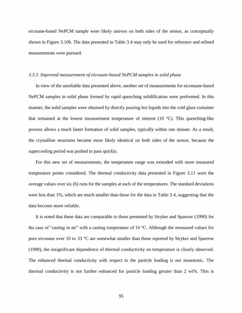
95
eicosane-based NePCM sample were likely uneven on both sides of the sensor, as conceptually
shown in Figure 3.10b. The data presented in Table 3.4 may only be used for reference and refined
measurements were pursued.
3.3.3 Improved measurement of eicosane-based NePCM samples in solid phase
In view of the unreliable data presented above, another set of measurements for eiconsane-based
NePCM samples in solid phase formed by rapid quenching solidification were preformed. In this
manner, the solid samples were obtained by directly pouring hot liquids into the cold glass container
that remained at the lowest measurement temperature of interest (10 °C). This quenching-like
process allows a much faster formation of solid samples, typically within one minute. As a result,
the crystalline structures became more likely identical on both sides of the sensor, because the
supercooling period was pushed to pass quickly.
For this new set of measurements, the temperature range was extended with more measured
temperature points considered. The thermal conductivity data presented in Figure 3.11 were the
average values over six (6) runs for the samples at each of the temperatures. The standard deviations
were less than 1%, which are much smaller than those for the data in Table 3.4, suggesting that the
data become more reliable.
It is noted that these data are comparable to those presented by Stryker and Sparrow (1990) for
the case of ―casting in air‖ with a casting temperature of 10 °C. Although the measured values for
pure eicosane over 10 to 33 °C are somewhat smaller than those reported by Stryker and Sparrow
(1990), the insignificant dependence of thermal conductivity on temperature is clearly observed.
The enhanced thermal conductivity with respect to the particle loading is not monotonic. The
thermal conductivity is not further enhanced for particle loading greater than 2 wt%. This is

96
consistent with the observed similar phenomenon for solid cyclohexane-based NePCM samples
(Figure 3.7b). At constant temperatures, the values for 5 and 10 wt% samples are similar to those
for 1 and 2 wt%, respectively. The greatest enhancement of about 9% relative to pure eicosane is
observed for the 2 and 10 wt% samples at 20 °C. This non-monotonic variation indicates the
possible existence of an optimum value of the loading of nanoparticles between 2 and 10 wt%,
although no physical reason was sought in the present study.
In addition, as temperature was further increased to 35 °C, thermal conductivity was markedly
enhanced. The possible reason for this anomalous enhancement is that solid eicosane was about to
start melting at this temperature and hence, the crystalline structures became unstable. During the
measurements, as heat was applied to the solid, melting might have happened in the vicinity of the
sensor, making the measurements even more complicated.
3.4 Summary
Thermal conductivity of cyclohexane- and eicosane-based NePCM samples containing
different loadings of sodium-oleate-stabilized CuO nanoparticles was measured experimentally
using the TPS technique. The NePCM samples were prepared with various loadings of
nanoparticles. With the aid of a controllable constant-temperature bath, measurements were
performed at multiple temperatures for both liquid and solid samples. The dependence of thermal
conductivity on both temperature and loading of nanoparticles was investigated.
For cyclohexane-based NePCM samples, the liquid thermal conductivity was inversely
related to temperature. Monotonic enhancement with increasing loading of nanoparticles was
observed in the liquid phase. The thermal conductivity value in the solid phase, however, was

97
proportionally dependent on temperature. It was also shown that the thermal conductivity of the
4 wt% samples is smaller than those for the 1 and 2 wt% samples, indicating a non-monotonic
enhancement phenomenon.
In the liquid phase, similar trends were observed for the eicosane-based NePCM samples.
The thermal conductivity decreased with increasing temperature, and increased with increasing
loading of nanoparticles, which fits to the Maxwell’s equation. The greatest enhancement was
found to be nearly 7% for the most concentrated sample (10 wt%) at 60 °C. Based on the
measured data, a simple linear correlation for thermal conductivity of liquid eicosane-based
NePCM colloids in relation to the loading of nanoparticles was proposed. Furthermore, the
measured thermal conductivity of eicosane-based NePCM samples in solid phase was shown to
be significantly dependent on the formation route of the solid samples. The results associated
with the slow solidification approach exhibited higher values of standard deviations among
individual runs for the same samples. This was reasoned to be related to the uneven solidified
structures on both sides of the sensor that are required to be identical by the TPS theory.
The rapid quenching solidification scheme was then attempted, which clearly led to more
stable results. Similar to the non-monotonic enhancement phenomenon observed for the
cyclohexane-based samples, enhancement of thermal conductivity was also not monotonic with
respect to the loading of nanoparticles, as the greatest enhancement was found for the 2 and 10
wt% samples (~9% at 20 °C). It was also shown that the thermal conductivity values exhibited a
marked increase when the measurement temperature approaches the melting point. This was
likely attributed to melting in the vicinity of the sensor as heat was applied during the
measurement periods.

98
Table 3.1 Density, latent heat of fusion and phase change temperatures of cyclohexane and
eicosane in their liquid phase
Property
Cyclohexane (C6H12)
(Sulfredge et al., 1993)
Eicosane (C20H42)
(http://msds.chem.ox.ac.uk/EI/eico
sane.html, and Hale et al., 1971)
(kg/m3) 779 789
L (J/kg) 32,557 247,000
Tm (Tf) (C) 6.5 ~37

99
Table 3.2 Specifications of the Hot Disk Thermal Constants Analyser (TPS 500)
Materials solids,
medium to high viscosity liquids,
small particles/powders
Thermal conductivity 0.03~100 W/mK
Thermal diffusivity 0.02~40 mm2/s
Specific heat capacity 0.10~4.5 MJ/m3K
Measurement time 2.5~640 seconds

100
Table 3.3 Measured thermal conductivity (unit: W/mK) of purified water at room
temperature and atmospheric pressure
Run number Test #1 Test #2
1 0.59614 0.60019
2 0.59970 0.61013
3 0.59967 0.60059
4 0.59593 0.59978
5 0.59570 0.60188
6 0.59394 0.60041
7 0.59641 0.60375
8 0.60348 0.60051
9 0.59036 0.59013
10 0.59935 0.60460
Average value (standard deviation) 0.59707 (± 0.364%) 0.60120 (± 0.500%)

101
Table 3.4 Measured thermal conductivity (unit: W/mK) of eicosane-based NePCM samples
in solid phase
Temperature (°C) 0 wt% 1 wt% 2 wt% 5 wt% 10 wt%
20 0.4236 0.4197 0.3386 0.3719 0.3422
30 0.3866 0.3664 0.3206 0.3333 0.3328
35 0.6608 0.9975 0.8161 0.7841 0.9695

102
(a)
(b)
Figure 3.1 Ball-and-stick molecular models of (a) cyclohexane (C6H12) and (b) eicosane (C20H42) with black and white balls
representing the carbon and hydrogen atoms, respectively

103
O
O
O
O
OO
O
O
O
O
O
O
O O
O
O
Figure 3.2 Schematic diagram of a nanoparticle with long ligands coated on its surface as the
stabilizing cushion layer (Clary and Mills, 2010)
stabilizing ligands (SOA, C18H33NaO2)
nanoparticle

104
Figure 3.3 TEM image of the synthesized sodium-oleate-stabilized CuO nanoparticles
(Reprinted with permission from Clary and Mills, 2011. Copyright 2011 American Chemical
Society)

105
Figure 3.4 Photograph of eicosane-based NePCM samples (in liquid phase) with various
mass fractions (0, 1, 2, 5 and 10 wt%) of CuO nanoparticles
0 wt% 1 wt% 10 wt% 2 wt% 5 wt%

106
Figure 3.5 A double-spiral-shaped hot disk sensor used in the TPS instruments
r

107
Figure 3.6 Arrangement of the experimental setup for measuring thermal conductivity of
NePCM samples
TPS Sensor
Constant-temperature bath
Aluminum holder
Glass container

108
Figure 3.7 Measured thermal conductivity of cyclohexane-based NePCM samples in both (a)
liquid and (b) solid phases as a function of temperature

109
Figure 3.8 Measured thermal conductivity of eicosane-based NePCM samples in liquid phase
as a function of temperature

110
Figure 3.9 Relative thermal conductivity of eicosane-based NePCM samples in liquid phase as
a function of the mass fraction of nanoparticles

111
Figure 3.10 Schematic diagrams of (a) the ideal arrangement with uniform materials on both
sides of the TPS sensor and (b) the realistic uneven structures associated with the relatively slow
formation of the solid sample
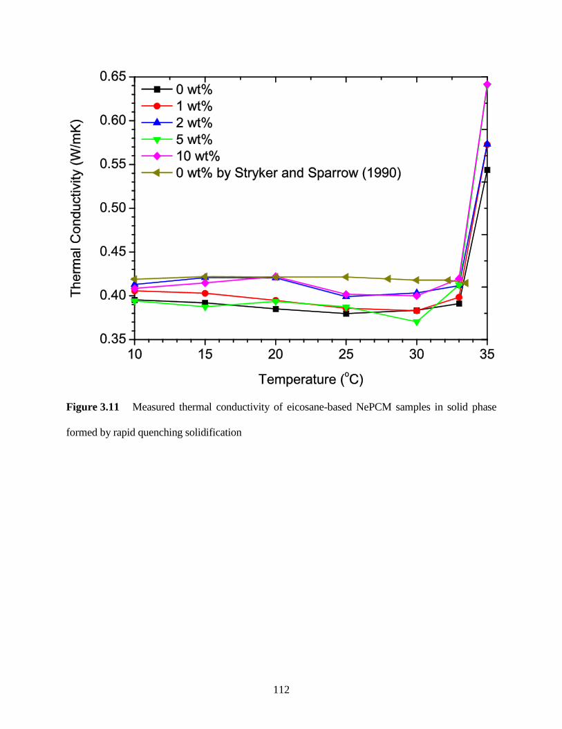
112
Figure 3.11 Measured thermal conductivity of eicosane-based NePCM samples in solid phase
formed by rapid quenching solidification

113
Chapter 4 Mathematical Modeling of Expedited Unidirectional Freezing of NePCM
In this chapter, mathematical modeling directed at quantifying the expedited unidirectional
freezing of NePCM is presented. Both the combined analytic/integral and the lattice Boltzmann
solutions to the one-dimensional, two-region Stefan problem in a finite slab are presented in
detail, followed by an application of the analytic solution to two representative cases of aqueous
and cyclohexane-based NePCM with various metal and metal oxide nanoparticles.
4.1 One-Dimensional Two-Region Stefan Problem
4.1.1 Fundamental assumptions for the Stefan problem
The Stefan problem is part of a broad family of partial differential equations (PDE) with
moving boundaries, which is named after Joseph Stefan who introduced this problem in relation
to the study of ice formation in 1890 (Gupta 2003). The Stefan problem is set up to model
transient heat conduction/diffusion involving melting/freezing. Due to the existence of a moving
boundary, the Stefan problem is inherently nonlinear and involves an unknown that is the region
to be solved, i.e., the location of the phase interface. A bibliography of research activities on the
Stefan problem is given by Tarzia (2000).
The mathematical formulation of the posed Stefan problem is based on some fundamental
assumptions, which are listed as follows:

114
1) The phase change process is governed by conservation of energy and the only transport
mechanism is due to heat conduction in both phases. Fluid flow associated with
convection is excluded.
2) The thermophysical properties of the PCM are constant but distinctly different in both
phases, including density, thermal conductivity and specific heat capacity. The latent heat
of fusion released at the interface is also constant.
3) The freezing temperature of the PCM is fixed and is only associated with the PCM.
4) The moving phase interface is sharp and is of zero thickness mathematically.
5) The supercooling and nucleation associated with freezing are neglected, i.e., freezing
happens immediately after the temperature has gone below the freezing point. Modeling
of supercooling effect upon solidification of PCM has been attempted by many
researchers, e.g., Günther et al. (2007).
6) The surface tension effect and curvature of the phase interface are also disregarded. For
example, for a one-dimensional freezing process, the phase interface is planar.
The simplest case is the 1-D one-region Stefan problem. For freezing, if it is assumed that the
initial temperature is at the freezing point (no subcooling) of the liquid PCM, the problem is
reduced to one-region such that the liquid will remain isothermal. Therefore, no heat conduction
will happen in the liquid and only conduction through the frozen layer needs to be considered,
for which an exact Stefan solution is available.
Considering heat conduction in both phases, the problem involves two regions that are
described by the Fourier’s equations with distinct properties for each phase. For the two-region
problem in a semi-infinite slab, an explicit solution is available, i.e., the Neumann’s solution. If

115
the slab has a finite thickness, however, no explicit solution is available and an
approximate/numerical technique is required to solve the problem.
4.1.2 Physical model for freezing of NePCM
The 1-D, two-region Stefan problem in a finite slab was considered in the present study.
Although the Stefan problem formulation is applicable for both melting and freezing, the effort
was only dedicated to investigation of freezing of NePCM, because natural convection is always
accompanied with melting, however, it is generally neglected during freezing. Therefore, the
Stefan model that excludes natural convection would be more realistic for modeling a freezing
process. Moreover, an experimental investigation on conduction-dominated freezing of NePCM
was planned to validate the Stefan model.
The physical model of the 1-D heat conduction of NePCM with unidirectional freezing is
schematically shown in Figure 4.1. An NePCM in its liquid phase occupies an infinitely large
space of finite thickness (0 ≤ x ≤ b). The initial uniform temperature (Ti) is above the freezing
point of the NePCM (Tf), which is assumed to be identical to that of the base PCM. For t > 0, the
boundary at x = 0 is held at a constant temperature (T0) that is below Tf, whereas the boundary at
x = b is kept insulated.
As shown in Figure 4.1a, freezing of the NePCM is initiated at the left boundary (x = 0) and
the solid-liquid interface will sweep through the slab toward the right insulated boundary. As
mentioned before, the phase interface is assumed to be planar and of zero thickness. Convection
driven by density variation in the liquid due to the presence of temperature gradient is also
neglected. The instantaneous position of the interface s(t), which is the thickness of the frozen
layer, is an unknown in this moving boundary problem. The frozen layer is subcooled except for

116
the phase interface that is at the freezing point. A portion of the heat that is transferred from the
region of interest is used to cool the shrinking liquid region. In effect, the temperature of the
insulated boundary at x = b will decrease, whereas the liquid at the interface is cooled to the
freezing point and latent heat of fusion is removed. The remaining portion of heat leaving at x =
0 serves to subcool the growing frozen layer. A typical transient temperature profile in both
phases at an early phase during the freezing process is presented in Figure 4.1b, where the
dimensionless quantities involved will be defined in the following section. Note that the left and
interface temperatures are always T0 and Tf, respectively, whereas the temperature of the right
interface will be continually lowered from its initial value of Ti after a certain time instant.
In this model, the NePCM was treated as a ―single-phase‖ homogeneous material such that
the introduction of nanoparticles into the base PCM only alters the effective thermophysical
properties. The dynamic diffusion of nanoparticles and their interaction with the moving phase
interface were not taken into consideration.
4.1.3 Mathematical formulation
The Stefan problem is mathematically formulated as follows. Firstly, the heat conduction
equation for the solid frozen layer is given by:
2
s
2
ss ),(),(
x
txT
t
txT
, for )(0 tsx and 0t , (4.1)
subject to the boundary condition:
0s ),( TtxT , at 0x and 0t . (4.2)
Concurrently, the governing equation for the liquid layer and the boundary condition are:
2
l
2
ll ),(),(
x
txT
t
txT
, for bxts )( and 0t , (4.3)

117
0),(l
x
txT, at bx and 0t . (4.4)
In the governing equations, the thermal diffusivities of both phases (s and l) are assumed
to be constant. The initial condition, which is only applicable for the liquid layer, is:
il )0,( TxT , for bx 0 . (4.5)
In addition, the temperature continuity and the Stefan condition at the solid-liquid interface
are given by:
fls ),(),( TtxTtxT , at )(tsx and 0t , (4.6)
dt
tdsL
x
txTk
x
txTk
)(),(),(s
ll
ss
, at )(tsx and 0t , (4.7)
Definitions of the symbols and subscripts are given in the Nomenclature. It is noted that the
density for the solid phase is used in the Stefan condition, i.e., Eq. (4.7), as an approximation for
considering the density variation at the interface upon freezing. The density for liquid phase
should be used if a melting problem is considered. Details of the derivation of the Stefan
condition have been presented by Jiji (2009).
Prior to non-dimensionalization of the above equations and the associated conditions, a group
of dimensionless quantities is defined at the outset:
b
xX ,
b
sS ,
2
s
b
t , and
0i
0
TT
TT
. (4.8)
Consequently, the dimensionless governing equation and the boundary condition for the
frozen layer are given by:
),(),( s
2
s
2 X
X
X, for )(0 SX and 0 , (4.9)
0),(s
X , at 0X and 0 . (4.10)

118
Similarly, the dimensionless governing equation and the boundary conditions for the liquid
layer are:
),(),( l
l
s
2
l
2 X
X
X, for 1)( XS and 0 , (4.11)
0),(l
X
X , at 1X and 0 . (4.12)
The dimensionless initial condition is:
1)0,(l X , for 10 X . (4.13)
In addition, the dimensionless interfacial conditions are:
fls ),(),( XX , at )(SX and 0 , (4.14)
d
dS
X
X
k
k
X
X )(
Ste
),(),( fl
s
ls
, at )(SX and 0 , (4.15)
where the Stefan number is defined as Ste = Cps(Tf – T0)/L, which is the governing dimensionless
quantity for the rate of a freezing process.
The above model depends on the thermal conductivity ratio (kl/ks), thermal diffusivity ratio
(l/s), Stefan number (Ste) and dimensionless freezing temperature (f). Therefore, the model is
capable of handling the variations of thermophysical properties of NePCM on both sides of the
liquid/solid interface. Because the exact solution cannot be obtained for the above equations, an
approximate or numerical solution has to be sought. In the following sections, the solutions
based on both the integral technique and lattice Boltzmann method (LBM) will be attempted.
4.2 Combined Analytic and Integral Method

119
Utilizing a combined analytic/integral methodology will lead to an approximate solution to
this 1-D, two-region Stefan problem in a finite slab, as presented by Cho and Sunderland (1969).
The details of the approach following the symbols adopted by Özışık (1980) are presented.
4.2.1 Analytic solution in the frozen layer
Following the Neumann’s similarity solution (Özışık, 1980), an explicit solution for the
governing equation in the frozen layer is obtained:
)(erf
)2(erf),(
f
s
XX , (4.16)
and the location of the interface S() is assumed to take the following form:
2)( S , (4.17)
where the parameter is to be determined.
4.2.2 Integral solution in the liquid layer
No exact solution is available for the temperature distribution in the liquid phase, unless an
infinite slab is considered. Thus, an integral method is adopted in order to assist in evaluation of
the quantity . In effect, a thermal layer () that is measured from X = 0, as shown in Figure
4.1b, is introduced for applying the integral method. It is assumed that the temperature in the
liquid zone beyond the thermal layer (X > ()) remains unaffected, i.e., isothermal at the initial
temperature. The validity of thermal layer over the entire freezing process is questionable since
when () reaches 1, the dimensionless temperature at the right boundary will drop below the
initial value. Thus, the thermal layer idea is just a convenient approach to determine . Given the
above reasoning, the boundary conditions at the edge of the thermal layer are:
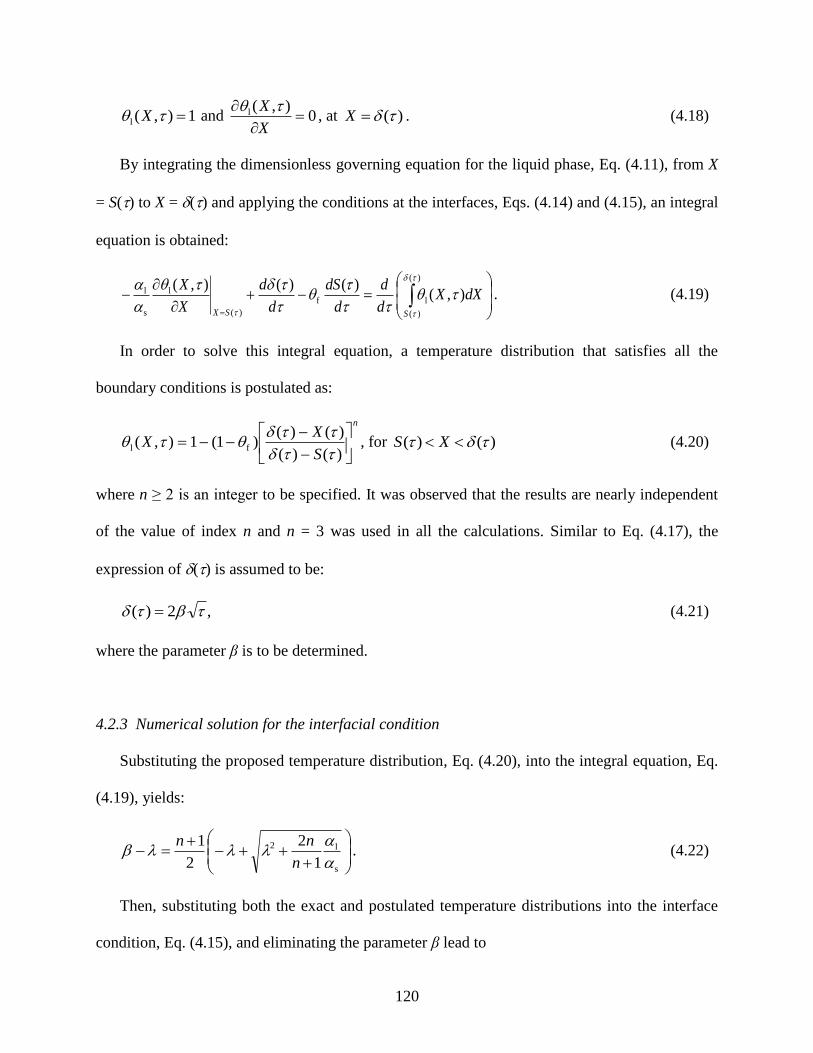
120
1),(l X and 0),(l
X
X , at )(X . (4.18)
By integrating the dimensionless governing equation for the liquid phase, Eq. (4.11), from X
= S() to X = () and applying the conditions at the interfaces, Eqs. (4.14) and (4.15), an integral
equation is obtained:
)(
)(
lf
)(
l
s
l ),()()(),(
SSX
dXXd
d
d
dS
d
d
X
X. (4.19)
In order to solve this integral equation, a temperature distribution that satisfies all the
boundary conditions is postulated as:
n
S
XX
)()(
)()()1(1),( fl
, for )()( XS (4.20)
where n ≥ 2 is an integer to be specified. It was observed that the results are nearly independent
of the value of index n and n = 3 was used in all the calculations. Similar to Eq. (4.17), the
expression of () is assumed to be:
,2)( (4.21)
where the parameter β is to be determined.
4.2.3 Numerical solution for the interfacial condition
Substituting the proposed temperature distribution, Eq. (4.20), into the integral equation, Eq.
(4.19), yields:
s
l2
1
2
2
1
n
nn. (4.22)
Then, substituting both the exact and postulated temperature distributions into the interface
condition, Eq. (4.15), and eliminating the parameter β lead to

121
0Ste
π11
)(erf f
f
l
s
s
l
2
Zk
ke, (4.23)
where
1
2
π
1
l
s2
l
s
n
n
n
nZ
. (4.24)
Since Eq. (4.23) is a transcendental equation, the parameter has to be determined by
numerical root-finding. Once is found, the dimensionless location of the interface S() and the
temperature distributions in both liquid and solid layers are obtained as well. Consequently,
based on Eq. (4.17), the dimensionless elapsed time for the freezing front to reach a given
position S is predicted by:
2
2
4
S . (4.25)
If the thermophysical properties of the NePCM and the parameters associated with the
problem, e.g., the initial and boundary temperature conditions, are given, this approximate
solution can be readily used. The MATLAB code that employs a numerical root-finding routine
based on the Newton-Raphson algorithm (Quarteroni et al., 2007) for solving Eq. (4.23) is given
in Appendix A. Overall simplicity of the above formulation and ease of implementation stand
out as the greatest advantages of this approximate solution.
4.3 Lattice Boltzmann Method (LBM)
4.3.1 Principle of the LBM for fluid flow
An emerging computational fluid dynamics (CFD) technique, the non-continuum-based
lattice Boltzmann method (LBM) has found broad applications in fluid flow and heat transfer

122
problems. The LBM has been proven to be a powerful alternative to the conventional CFD
techniques, e.g., finite volume and finite element methods, that are used for solving macroscopic
continuum governing equations, e.g., Navier-Stokes equations.
Originated from the lattice gas automata (LGA), the LBM is fulfilled based on mesoscopic
kinetic evolution equations (Wolf-Gradrow, 2000), i.e., the Boltzmann equation. The
macroscopic characteristics of a physical system under consideration are simulated by the
evolution of the particle distribution functions at discrete particles (lattices) in the system. The
principle and implementation of the LBM in fluid mechanics problems are available in the
literature (e.g., Chen and Doolen, 1998, Wolf-Gradrow, 2000, and Succi, 2001). The classical
continuum Boltzmann equation, which is in the form of an integral-differential equation, for a
single particle distribution function (f(x, t)) is given by
)(),(),(
ftft
tf
xv
x, (4.26)
where x is the particle position vector, v the particle velocity, and the collision integral.
The Bhatnagar-Gross-Krook (BGK) approximation (Succi, 2001) has been the most popular
scheme to simplify the collision term on the right-hand side of Eq. (4.26), which leads to
),(),(1
),(),( Eq tftftf
t
tfxxxv
x
, (4.27)
where is the relaxation time and fEq
(x, t) is the equilibrium distribution function that satisfies
the Maxwell-Boltzmann distribution. If the particle distribution is considered to evolve in
uniform lattices with finite discrete velocity directions (total number of m), the equation for each
direction is given by:
),(),(1
),(),( Eq
tftftft
tfiiii
i xxxex
, (4.28)

123
where subscript i denotes the ith-direction of discrete velocity component (i = 0, 1,…, m – 1),
and e the lattice velocity vector.
Discretization of the Eq. (4.28) in space (x) and time (t) leads to
),(),(1),(),(),(),( Eq
tftft
ttftttf
t
tfttfii
i
iii
i
ii xxe
xexe
xx
, (4.29)
where the relation x = eit has already been used. The above equation is further simplified to
),(),(1
),(),( Eq tftftftttfiiiii
xxxex
, (4.30)
where = /t is the dimensionless relaxation time.
The above equation, Eq. (4.30), is called the LBGK equation that is the lattice Boltzmann
equation with BGK approximation for the collision term. This equation is expressed in the form
that consists of distinct parts on both sides. The left-hand side stands for the streaming step,
whereas the right-hand side denotes the collision step. In the computer algorithm, these two steps
only require explicit operations, which stands out as the primary advantage of the LBM over
classical CFD methods.
A number of geometric lattice models have been proposed in the literature. It is customary to
denote the models as DnQm, with n and m being the spatial dimension and the number of
velocity directions at each lattice, respectively. Obviously, for the simplest 1-D case, the D1Q2
model is the rational option. However, when it comes to higher dimensions, many candidate
geometries are available as long as the symmetry is satisfied. Due to the simplicity and ease of
formulation, square and cubic models have dominated in 2-D and 3-D cases, respectively. As an
example, the widely used 2-D model, D2Q9, is presented schematically in Figure 4.2.
It is shown that in the square lattice three types of particles exist, which are the rest particle
(0) in the lattice kernel, four particles moving along horizontal and vertical directions (1, 2, 3,
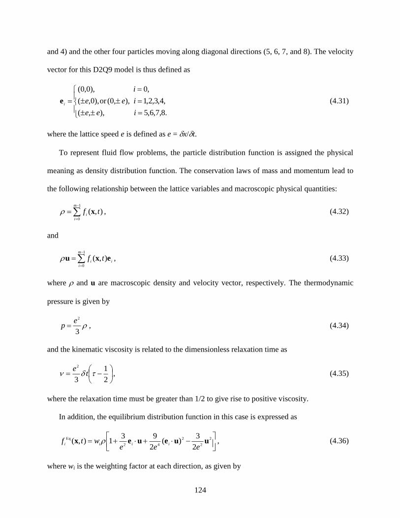
124
and 4) and the other four particles moving along diagonal directions (5, 6, 7, and 8). The velocity
vector for this D2Q9 model is thus defined as
.8,7,6,5),,(
,4,3,2,1),(0,or),0,(
,0),0,0(
iee
iee
i
ie (4.31)
where the lattice speed e is defined as e = x/t.
To represent fluid flow problems, the particle distribution function is assigned the physical
meaning as density distribution function. The conservation laws of mass and momentum lead to
the following relationship between the lattice variables and macroscopic physical quantities:
1
0
),(m
ii
tf x , (4.32)
and
i
m
ii
tf exu
1
0
),( , (4.33)
where and u are macroscopic density and velocity vector, respectively. The thermodynamic
pressure is given by
3
2ep , (4.34)
and the kinematic viscosity is related to the dimensionless relaxation time as
2
1
3
2
te
, (4.35)
where the relaxation time must be greater than 1/2 to give rise to positive viscosity.
In addition, the equilibrium distribution function in this case is expressed as
2
2
2
42
Eq
2
3)(
2
931),( uueuex
eeewtf
iiii , (4.36)
where wi is the weighting factor at each direction, as given by

125
.8,7,6,5,36/1
,4,3,2,1/9,1
,0,9/4
i
i
i
wi
(4.37)
It is noted that the summation of the weighting factors over the subscripts is equal to unity.
As such, the LBGK model to simulate 2-D fluid flow problems with Newtonian fluids is
established. The recovery of the Navier-Stokes equations from the LBGK equation has been
shown by using the Chapman-Enskog expansion (Hou et al., 1995). To apply the LBM, the
knowledge of boundary conditions is also needed. The most common non-slip condition on a
wall used in LBM is the so-called ―bounce-back‖ boundary condition. Details of application of
various types of boundary conditions are available in the literature (e.g., Zou and He, 1997).
4.3.2 Thermal LBM (TLBM)
Furthermore, thermal LBM (TLBM) that is applied to solve non-isothermal fluid flow and
thermodynamic problems has also been proposed (e.g., Chen et al., 1995). There have been two
main approaches for TLBM models: the multi-speed and multiple distribution function. The
former introduces additional discrete velocities in lattices to simulate energy conservation,
whereas the latter uses an individual particle distribution function (h(x, t)) to represent energy.
The multiple distribution function approach has stood out as it provides rational stability and
requires the same effort as that for implementation of isothermal LBM.
Obviously, the multiple distribution function approach assumes that the energy distribution
function is subjected to the same evolution equation for density distribution function. This is
verified if the viscous heating and compression work effects are neglected in the macroscopic
energy equation. The TLBM is thus able to recover to the macroscopic energy equation with

126
temperature as the transport scalar, analogous to density for isothermal LBM. The TLBM for the
energy distribution function subjected to BGK approximation is given by
),(),(1
),(),( Eq thththttthiiiii
xxxex
, (4.38)
where is the dimensionless relaxation time for energy.
The temperature at each lattice is obviously evaluated as
1
0
),(m
ii
thT x , (4.39)
and the thermal diffusivity is given by
2
1
3
2
te
. (4.40)
In combination with the relation for kinematic viscosity, Eq. (4.35), the Prandtl number for a
Newtonian fluid is defined as
12
12Pr
. (4.41)
which apparently becomes a tunable variable.
Moreover, the equilibrium energy distribution function becomes
2
2
2
42
Eq
2
3)(
2
931),( uueuex
eeeTwth
iiii. (4.42)
It is noted that the TLBM could be implemented on separate lattice model with the
isothermal LBM. Furthermore, if the problem under consideration reduces to a pure heat
conduction problem, i.e., convection is absent, the TLBM works individually and the equilibrium
distribution function is simplified to
Twthii
),(Eqx . (4.43)

127
In this case, the heat conduction equation without an energy source term will be recovered
from the TLBM model by using the Chapman-Enskog expansion. Additionally, there are two
types of boundary conditions for heat conduction problems: specified wall temperature and wall
heat flux. The adiabatic boundary condition is absorbed in the latter if a zero wall heat flux is
applied. The application of these two types of boundary conditions will be presented below as
both appear in the 1-D Stefan model.
4.3.3 Extended TLBM for heat conduction with phase change
The moving boundary problems have been solved numerically on fixed grids by adopting the
enthalpy-based formulation of thermal energy (Shyy et al., 1996). The enthalpy formulation to
solve the Stefan problem has been presented in the literature (e.g., White, 1982 and Cesari,
1992). In the enthalpy-based framework, the 1-D transient heat conduction equation, e.g., Eqs.
(4.1) and (4.3), may be written as
2
2
x
Tk
t
H
, (4.44)
where the total enthalpy for a PCM undergoing solid-liquid phase change is defined as the
summation of both sensible and latent heat (of fusion), as given by:
LdTCHp
. (4.45)
where is introduced as the fraction of liquid phase and its value varies between 0 and 1.
By substituting Eq. (4.45) into Eq. (4.44), it is manipulated to
2
2
x
Tk
tL
t
TC
p
, (4.46)
which is further rearranged to

128
tC
L
x
T
t
T
p
2
2
, (4.47)
It is noted that the latent heat of fusion appears in Eq. (4.47) as a source term and the rest of
the equation recovers the heat conduction equation. Assuming that the PCM possesses a fixed
freezing point, the relationship between the enthalpy and temperature is established by
.,
,,
),(,
f
fff
ff
LHHC
LH
LHHHT
TCHHC
H
T
p
p
p
(4.48)
where Hf is the enthalpy corresponding to the PCM at its freezing point. Hence, the constitutive
relationship between the liquid fraction and temperature is given by
.1,
,,
,,0
f
f
f
f
TT
TTL
HH
TT
(4.49)
Given the above relation, the governing equations are closed and the liquid fraction can be
solved simultaneously with temperature as part of the numerical solution.
Recall that the thermal LBGK equation is able to recover the heat conduction equation
without a source term. In view of this, an extension of the LBGK equation to represent heat
conduction with a source term, e.g., Eq. (4.47), becomes straightforward. The extension of
LBGK equation to solve phase change heat conduction was first proposed by Jiaung et al. (2001)
and the application of the extended TLBM to solve 1-D and 2-D melting/freezing problems was
presented. Chatterjee and Chakraborty (2005) demonstrated the application of such extended
LBM model to solve 3-D conduction-dominated phase change problems. More recently, Huber
et al. (2008) presented the utilization of such method in cooperation with isothermal LBM to

129
solve melting heat transfer involving natural convection. In the present study, attention was only
paid to heat conduction with phase change and hence, the Jiaung’s model was used. First, the
extended LBGK equation with an additional source term reads
iiiiii
tthththttth
),(),(1
),(),( Eqxxxex , (4.50)
where the discrete source term satisfies
ii
w . (4.51)
Jiaung et al. (2001) showed that this extended LBGK equation is able to recover the heat
conduction equation, Eq. (4.47), only if the source term takes the form as
tC
L
p
, (4.52)
The final discretized form of the extended LBGK equation is given by
)()(),(),(1
),(),( Eq tttC
Lwthththttth
p
iiiiii
xxxex , (4.53)
After specifying the boundary conditions, the above equation is solved as usual. However,
due to the presence of the additional source term, an internal iteration procedure is required
during each time step to solve for the local liquid fraction at all the lattices. The detailed solution
procedure was outlined by Jiaung et al. (2001). Here the pseudo code that demonstrates the
solution procedure in the computer algorithm is presented in Figure 4.3.
4.3.4 The LBM solution for the 1-D Stefan problem
In the previous section, the extended LBGK model was presented based on the D2Q9 model
for 2-D applications. To apply the LBM solution for the proposed 1-D Stefan model, the D1Q2
lattice model should be used. The schematic diagram of a D1Q2 model with uniform lattice is
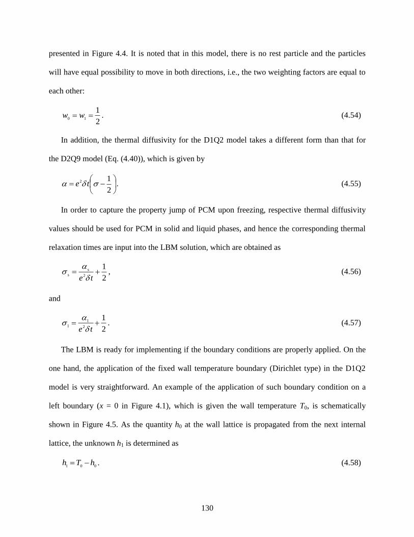
130
presented in Figure 4.4. It is noted that in this model, there is no rest particle and the particles
will have equal possibility to move in both directions, i.e., the two weighting factors are equal to
each other:
2
110 ww . (4.54)
In addition, the thermal diffusivity for the D1Q2 model takes a different form than that for
the D2Q9 model (Eq. (4.40)), which is given by
2
12 te . (4.55)
In order to capture the property jump of PCM upon freezing, respective thermal diffusivity
values should be used for PCM in solid and liquid phases, and hence the corresponding thermal
relaxation times are input into the LBM solution, which are obtained as
2
12
s
s
te
, (4.56)
and
2
12
l
l
te
. (4.57)
The LBM is ready for implementing if the boundary conditions are properly applied. On the
one hand, the application of the fixed wall temperature boundary (Dirichlet type) in the D1Q2
model is very straightforward. An example of the application of such boundary condition on a
left boundary (x = 0 in Figure 4.1), which is given the wall temperature T0, is schematically
shown in Figure 4.5. As the quantity h0 at the wall lattice is propagated from the next internal
lattice, the unknown h1 is determined as
001hTh . (4.58)

131
On the other hand, the application of the prescribed wall heat flux boundary condition
(Neumann type) becomes much more complicated. As proposed by Jiaung et al. (2001), a
control-volume-type method was used to derive the boundary condition. As schematically shown
in Figure 4.6, an example is given for the right boundary (x = b in Figure 4.1), where the wall
heat flux q is given. The control volume occupies the half lattice next to the wall. The heat flux
qin flowing into the control volume through the right wall is equal to the prescribed wall heat flux
q, whereas the heat flux flowing out is estimated by using the Fourier’s law, as given by
x
TTkq nn
)(1
out
. (4.59)
Taking an energy balance over the control volume leads to
dtqqdtdxt
TC
tt
t
tt
tp
)(outin
. (4.60)
which is numerically integrated to
)()(1
nn
t
n
tt
n
pTT
x
kqTT
t
xC
. (4.61)
For ease of implementation, an explicit treatment on the right-hand side of Eq. (4.61) yields
qTx
kT
x
k
t
xCT
t
xCt
n
t
n
ptt
n
p
122
, (4.62)
which is reduced to the adiabatic boundary condition when q vanishes.
As presented before, the LBM solution based on D1Q2 lattice model was established for
solving the 1-D Stefan model. As an example, the LBM model was used to solve an ice
formation problem, which was also solved by using the aforementioned integral technique for
comparison. The MATLAB code that implements the LBM solution for 1-D freezing heat
conduction is given in Appendix B. The ice formation process in a 2 mm thick slab was
132
considered with the physical model following exactly as that shown in Figure 4.1. The
parameters including the initial and boundary conditions of the problem under consideration are
listed in Table 4.1.
By implementing the MATLAB code given in Appendix B, the dynamic comparison of the
solutions was obtained. For the LBM solution, the lattice interval and time step size were set to
be x = 10–5
m and t = 10–4
s, respectively. There were 201 uniform lattice grids in the
computational domain and the computation proceeded for 10,000 time steps. After marching
1,000 time steps, the comparisons of the dimensionless temperature profile and location of
freezing front between both solutions are presented in Figure 4.7. It is clearly shown that the
results of both solutions agree well with each other. Little deviation is only found right at the
phase interface ( = 2/3), because the integral solution assumes a zero-thickness interface but the
LBM solution would take one grid to accommodate the interface over which the value of liquid
fraction is between 0 and 1 (see Eq. (4.49)).
As freezing proceeds, the thermal layer will reach the right insulated boundary earlier than
the phase interface does. It is noted that the integral solution would become invalid while the
thermal layer has reached the insulated boundary. Beyond that time instant, the integral solution
is no longer able to solve for the temperature profile in the remaining liquid layer. However, it is
noted that the exact solution in the frozen layer always works. For this specific problem, the
thermal layer was found to arrive at the right boundary after 9,745 time steps and the
comparisons at this time instant are presented in Figure 4.8. Excellent agreement is observed
except for the grid at which the phase interface is located. The applicability of the LBM solution
to the 1-D Stefan problem was therefore justified.
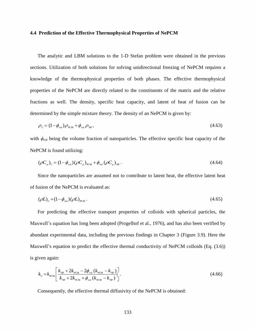
133
4.4 Prediction of the Effective Thermophysical Properties of NePCM
The analytic and LBM solutions to the 1-D Stefan problem were obtained in the previous
sections. Utilization of both solutions for solving unidirectional freezing of NePCM requires a
knowledge of the thermophysical properties of both phases. The effective thermophysical
properties of the NePCM are directly related to the constituents of the matrix and the relative
fractions as well. The density, specific heat capacity, and latent of heat of fusion can be
determined by the simple mixture theory. The density of an NePCM is given by:
NPvolPCMvolC)1( , (4.63)
with vol being the volume fraction of nanoparticles. The effective specific heat capacity of the
NePCM is found utilizing:
NPvolPCMvolC)()()1()(
pppCCC . (4.64)
Since the nanoparticles are assumed not to contribute to latent heat, the effective latent heat
of fusion of the NePCM is evaluated as:
PCMvolC)()1()( LL . (4.65)
For predicting the effective transport properties of colloids with spherical particles, the
Maxwell’s equation has long been adopted (Progelhof et al., 1976), and has also been verified by
abundant experimental data, including the previous findings in Chapter 3 (Figure 3.9). Here the
Maxwell’s equation to predict the effective thermal conductivity of NePCM colloids (Eq. (3.6))
is given again:
)(2
)(22
NPPCMvolPCMNP
NPPCMvolPCMNP
PCMCkkkk
kkkkkk
. (4.66)
Consequently, the effective thermal diffusivity of the NePCM is obtained:

134
C
CC
)( pC
k
. (4.67)
It is noted that the above equations are applied to both liquid and solid phases. For a given
volume fraction of nanoparticles, the above-mentioned effective thermophysical properties of the
NePCM can be readily predicted.
As discussed earlier, the LBM provides a numerical solution that will always be valid during
the entire freezing process. However, use of the analytic solution is easy to obtain the freezing
time of a given thickness of the slab. In this sense, the analytic solution was used to exhibit the
comparison of the rate of freezing for various NePCM. Nevertheless, if attention is paid on the
transient evolutions of temperature profiles and freezing front, the LBM solution is preferred.
4.5 Application of the Analytic Solution
4.5.1 Thermophysical properties and parameters
Two representative cases of water and cyclohexane (C6H12) as the base PCM with alumina
(Al2O3), copper (Cu), copper oxide (CuO), and titanium oxide (TiO2) nanoparticles were
considered. Five (5) different volume fractions (vol = 0, 1, 2, 5 and 10 vol%) of the
nanoparticles were studied. Given the thermophysical properties of the constituents and the
specified volume fractions, effective thermophysical properties of the NePCM colloids were
readily predicted using Eqs. (4.63) to (4.67), which are presented in Appendix C.
In the calculations, the initial temperature Ti was set to be 300 K, while the cold boundary
temperature (T0) was kept to be 20 °C below the respective freezing points for water (Tf = 0 °C)
and cyclohexane (Tf = 6.5 °C). As a result, the Stefan numbers for aqueous NePCM ranged
between 0.12 and 0.14, whereas for cyclohexane-based colloids the range was between 1.11 and

135
1.44. The dimensionless initial and boundary temperatures are i = 1 and 0 = 0, respectively. In
addition, the freezing time durations were predicted for a slab thickness of b = 0.05 m. As
indicated by Eqs. (4.23) and (4.24), given the Stefan number and dimensionless freezing
temperature, the freezing time duration is a function of the liquid to solid thermal conductivity
and diffusivity ratios of the NePCM. In the following sections, the effects of these ratios on the
freezing time durations will be presented.
4.5.2 Effect of the liquid to solid thermal conductivity ratio
If the dimensionless total freezing time for the slab of thickness b (i.e., S = 1) is considered,
Eq. (4.25) is obviously reduced to
2total 4
1
. (4.68)
Given the aforementioned parameters, the predicted dimensionless total freezing time total as
a function of the liquid to solid thermal conductivity ratio (kl/ks) for aqueous NePCM is
presented in Figure 4.9. Various colors and symbols are used to identify the volume fractions of
nanoparticles. Straight lines are also drawn through the appropriate computed quantities to
identify the specific materials of nanoparticles.
It is observed that the variation of the freezing time is almost linearly correlated to the
thermal conductivity ratio. For a constant volume fraction, the smallest and greatest variations of
the thermal conductivity ratio are realized by the colloids of high (Cu) and low (TiO2) thermal
conductivity nanoparticles, respectively. Moreover, for a given type of additive material, as the
loading of nanoparticles is raised, the thermal conductivity ratio increases.
Similarly, the predicted dimensionless total freezing times for cyclohexane-based NePCM
are presented in Figure 4.10. Regardless of the base PCM (water or cyclohexane), the smallest

136
and greatest variations of the thermal conductivity ratio are associated with the NePCM colloids
with Cu and TiO2 nanoparticles, which possess the highest and lowest thermal conductivity
among the four nanoparticles considered, respectively. The most interesting finding is that for a
given base PCM (i.e., water in Figure 4.9 and cyclohexane in Figure 4.10) and a constant value
of the volume fraction, the dimensionless freezing time is nearly constant and is independent of
the material of the suspended nanoparticles.
4.5.3 Effect of the liquid to solid thermal diffusivity ratio
The predicted dimensionless freezing times of the aqueous and cyclohexane-based NePCM
are presented in Figure 4.11 and Figure 4.12, respectively, in relation to the liquid to solid
thermal diffusivity ratio (l/s). In both figures, symbols and straight lines used in Figure 4.9 and
Figure 4.10 are adopted to identify the volume fractions and materials of nanoparticles,
respectively.
With water as the base PCM (Figure 4.11), the observed trends for the variation of the
dimensionless freezing time with respect to the thermal diffusivity ratio are analogous to those
discussed earlier for the effect of the thermal conductivity ratio. However, for cyclohexane-based
NePCM the increasing trends of the thermal diffusivity ratio with greater loading of the
nanoparticles is reversed, as observed in Figure 4.12. This is attributed to the opposite trends of
both density and specific heat capacity when the PCM transforms from the liquid to solid phase.
For water, both its density and specific heat capacity decrease upon freezing, whereas for
cyclohexane these properties increase. It is also noted that various curves for different types of
suspended nanoparticles collapse onto each other in Figure 4.12. Regardless of the opposite

137
trends exhibited by cyclohexane, expedited freezing that is afforded to the suspension of
nanoparticles and its direct relation to the volume fraction of the nanoparticles are maintained.
4.5.4 Expedited freezing rate
The average values of the predicted dimensionless total freezing times for a given volume
fraction of the nanoparticles for both aqueous and cyclohexane-based NePCM are summarized in
Table 4.2, in which the relative percentages of expediting in comparison to the case of the
particle-free PCM are also provided. It is shown that regardless of the type of suspended
nanoparticles, the aqueous and cyclohexane-based NePCM with a loading of nanoparticles of 10
vol% give rise to expedited freezing times by 11.4 and 6.9%, respectively.
As an example, the transient variations of the liquid fraction during the freezing process
(discharging) for aqueous NePCM with Al2O3 nanoparticles are presented in Figure 4.13. Faster
energy discharging rate is clearly exhibited as the loading of nanoparticles is increased. The
expedited thermal energy discharge exhibited by this representative NePCM points to its
potential as a superior thermal energy storage material.
The dimensionless wall heat flux at the cooling boundary (X = 0) can be derived from the
temperature distribution within the solid layer, Eq. (4.16), given by
1
)(erfπ
),(f
0
s
XdX
XdQ , (4.69)
which is obviously a time-dependent function. This quantity is the instantaneous heat flux
leaving the slab region of interest.
For the aqueous-Al2O3 NePCM samples, comparison of the transient variations of the wall
heat flux is presented in Figure 4.14. The heat flux values are extremely high at the very

138
beginning (τ = 0) and decay rapidly within τ < 1 period. Thereafter, the curves gradually decay as
freezing proceeds.
In light of the fact that the five curves nearly resemble to one another, an inset is introduced
in Figure 4.14 to assist close observation of the comparison among the curves between 0.5 < τ <
1. It is observed that at a given time instant, the heat flux is lowered with increased loading of
nanoparticles. This indicates that less dimensionless total power, estimated by the area under the
curve in Figure 4.14, is required to freeze the entire slab for NePCM with higher concentration of
nanoparticles, consistent with the predicted lowering of both effective specific heat capacity and
latent heat of fusion of the colloids in the presence of nanoparticles.
4.6 Summary
A 1-D, two-region Stefan problem was formulated to model unidirectional freezing of
NePCM in a finite slab. The problem was first solved using a combined analytic/integral
approach. The temperature profile in the growing solid layer was solved exactly, whereas the
integral method was applied to the liquid layer. A numerical-root finding algorithm was then
employed to solve the transcendental equation at the liquid/solid interface. The LBM was
proposed under the enthalpy-based framework. The original LBGK equation was extended by
introducing a source term to consider the variation of latent heat of fusion upon phase change.
The numerical results of the extended LBM was compared favorably to the analytic solution for
an ice formation problem and excellent agreement was shown.
By utilizing the analytic solution, unidirectional freezing of both aqueous and cyclohexane-
based NePCM with various nanaparticles were studied and the following conclusions were

139
drawn. As the volume fraction of the suspended nanoparticles was raised, the liquid to solid
thermal conductivity ratio for the colloids increased. Water and cyclohexane exhibited opposite
trends for dependence of the liquid to solid thermal diffusivity ratio in relation to introduction of
more nanoparticles. This was linked to the opposite trends of both density and specific heat
capacity when the PCM undergoes freezing. For a given base PCM and a constant volume
fraction, the dimensionless freezing time was nearly constant and was independent of the
material of the nanoparticles. Freezing became clearly faster as the loading of nanoparticles was
increased and the trend was found to be almost linear. For the representative aqueous NePCM,
an expediting of freezing up to 11.4% was observed by adding 10 vol% nanoparticles.

140
Table 4.1 Parameters in the ice formation problem for validating the LBM solution
Parameter Quantity
b 2 mm
Tf 0 °C
Ti 5 °C
T0 −10 °C

141
Table 4.2 Predicted dimensionless total freezing times and the corresponding percentages of
expediting (in parentheses) for aqueous and cyclohexane-based NePCM
Base PCM 0 vol% 1 vol% 2 vol% 5 vol% 10 vol%
water 6.9619
6.8859
(1.1%)
6.8083
(2.2%)
6.5706
(5.6%)
6.1711
(11.4%)
cyclohexane 1.6107
1.5975
(0.8%)
1.5849
(1.6%)
1.5507
(3.7%)
1.4995
(6.9%)

142
Figure 4.1 Schematic diagrams of (a) the physical model of the 1-D unidirectional freezing
of NePCM in a finite slab and (b) instantaneous dimensionless temperature profiles

143
Figure 4.2 Schematic diagram of the D2Q9 lattice model
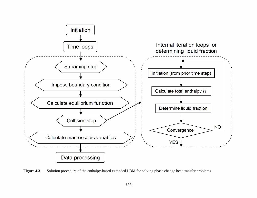
144
Figure 4.3 Solution procedure of the enthalpy-based extended LBM for solving phase change heat transfer problems

145
Figure 4.4 Schematic diagram of the D1Q2 lattice model

146
Figure 4.5 Schematic diagram of the application of fixed wall temperature boundary
condition in the D1Q2 lattice model

147
Figure 4.6 Schematic diagram of the application of a prescribed wall heat flux boundary
condition in the D1Q2 lattice model

148
Figure 4.7 Comparison of the dimensionless temperature profile and location of phase
interface between the LBM and analytic solutions after marching 1,000 time steps

149
Figure 4.8 Comparison of the dimensionless temperature profile and location of phase
interface between the LBM and integral solutions after marching 9,745 time steps
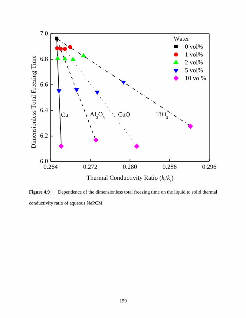
150
0.264 0.272 0.280 0.288 0.2966.0
6.2
6.4
6.6
6.8
7.0
TiO2
CuOAl2O
3
Water
0 vol%
1 vol%
2 vol%
5 vol%
10 vol%
Dim
ensi
on
less
To
tal
Fre
ezin
g T
ime
Thermal Conductivity Ratio (kl/k
s)
Cu
Figure 4.9 Dependence of the dimensionless total freezing time on the liquid to solid thermal
conductivity ratio of aqueous NePCM

151
0.9338 0.9340 0.9342 0.9344 0.93461.48
1.50
1.52
1.54
1.56
1.58
1.60
1.62
TiO2
CuO
Al2O
3
Cyclohexane
0 vol%
1 vol%
2 vol%
5 vol%
10 vol%
Dim
ensi
on
less
To
tal
Fre
ezin
g T
ime
Thermal Conductivity Ratio (kl/k
s)
Cu
Figure 4.10 Dependence of the dimensionless total freezing time on the liquid to solid thermal
conductivity ratio of cyclohexane-based NePCM

152
0.116 0.120 0.124 0.128 0.132 0.136 0.1406.0
6.2
6.4
6.6
6.8
7.0 Water
0 vol%
1 vol%
2 vol%
5 vol%
10 vol%
Dim
en
sio
nle
ss T
ota
l F
reezin
g T
ime
Thermal Diffusivity Ratio (l/
s)
CuAl
2O
3
CuO
TiO2
Figure 4.11 Dependence of the dimensionless total freezing time on the liquid to solid thermal
diffusivity ratio of aqueous NePCM

153
1.011 1.014 1.017 1.020 1.023 1.026 1.029 1.032 1.0351.48
1.50
1.52
1.54
1.56
1.58
1.60
1.62
Cyclohexane
0 vol%
1 vol%
2 vol%
5 vol%
10 vol%
Dim
en
sio
nle
ss T
ota
l F
reezin
g T
ime
Thermal Diffusivity Ratio (l/
s)
Figure 4.12 Dependence of the dimensionless total freezing time on the liquid to solid thermal
diffusivity ratio of cyclohexane-based NePCM
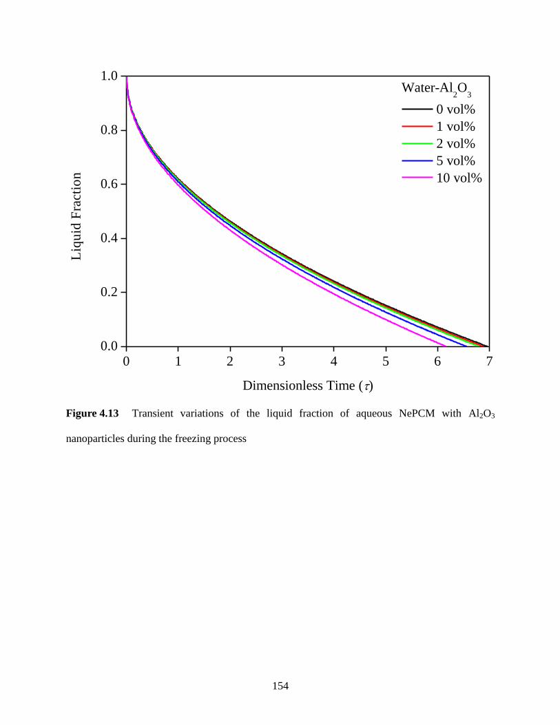
154
0 1 2 3 4 5 6 70.0
0.2
0.4
0.6
0.8
1.0L
iqu
id F
ract
ion
Dimensionless Time ()
Water-Al2O
3
0 vol%
1 vol%
2 vol%
5 vol%
10 vol%
Figure 4.13 Transient variations of the liquid fraction of aqueous NePCM with Al2O3
nanoparticles during the freezing process

155
0 1 2 3 4 5 6 70
1
2
3
4
5Water-Al
2O
3
0 vol%
1 vol%
2 vol%
5 vol%
10 vol%
Dim
en
sio
nle
ss W
all
Heat
Flu
x a
t X
= 0
Dimensionless Time ()
0.5 0.6 0.7 0.8 0.9 1.01.1
1.2
1.3
1.4
1.5
Figure 4.14 Transient variations of the dimensionless wall heat flux at the cooling boundary of
aqueous NePCM with Al2O3 nanoparticles during the freezing process
156
Chapter 5 Experimental Investigations of Expedited Unidirectional Freezing of NePCM
In this chapter, results of experimental investigations of unidirectional freezing of NePCM
are presented. An ice formation test using the original experimental setup employing a
thermoelectric cooler as the cooling source is discussed, followed by presentation of the results
on cyclohexane-based NePCM with stabilized copper oxide nanoparticles. The results of the
refined experimental setup employing a copper cold plate are then presented with an emphasis on
the system improvements compared to the previous work.
5.1 Unidirectional Freezing Experiment: A Test Case with Distilled Water
5.1.1 Experimental setup and instruments
In order to verify the expedited freezing of NePCM due to its enhanced thermal conductivity
and to provide experimental data for comparison with the 1-D Stefan model, a unidirectional
freezing experimental setup was designed, constructed, and tested, as schematically illustrated in
Figure 5.1. A cooled-from-bottom arrangement was adopted so as to avoid promotion of natural
convection in liquid during freezing (Boger and Westwater, 1967), since the density of a liquid is
generally inversely proportional to temperature. A thermally stable arrangement was therefore
established with the lighter liquid layer (warmer) on top of the heavier layer (colder). The
consequences of thermally unstable layers on phase change were briefly mentioned in Chapter 2

157
in relation to work of Henze and Humphrey (1981) and are also discussed in detail by Tan et al.
(2009).
By doing so, the freezing process was dominated only by conduction, which physically
matches the 1-D Stefan model, as shown in Figure 4.1. The test cell for containing the NePCM
sample was fabricated from a glass (Pyrex) tube with a square inner cross-section (24.8 24.8
mm2). The Pyrex glass possesses a thermal conductivity of approximately 1 W/mK at room
temperature (http://www.engineeringtoolbox.com/thermal-conductivity-d_429.html). The tube
was placed vertically, as shown in Figure 5.1a, and its bottom was sealed using a Teflon tape
(Thread seal tape, CFPC, Ningbo, CHINA) and a clear silicone sealant (Loctite, Henkel
Corporation, Avon, OH) against a 6.7 mm thick Al plate that served as the active cooling
boundary. To provide the cooling source, a square thermoelectric cooler (TEC) (Model No.
81628, FerroTec, Bedford, NH) with cross-sectional area of 22.4 22.4 mm2 was attached to the
bottom of the Al plate and was supported by a copper-cored aluminum-finned heat sink
underneath it. A fan was associated with the heat sink to provide active air cooling. The TEC
was powered by an adjustable DC power supply (Model No. 303, Proteck, TAIWAN). The
horizontal planar gaps between the Al plate, TEC, and the copper core of the heat sink were
filled with thin layers of thermal grease (FerroTec, Bedford, NH) to enhance the thermal contact
conductance. Moreover, in order to establish a quasi 1-D heat conduction path, a thick insulation
jacket made of Styrofoam (~0.033 W/mK, available at http://www.engineeringtoolbox.com/
thermal-conductivity-d_429.html) was used to tightly embrace the test cell on four (4) side walls.
The insulation also served to block exchange of heat between the freezing cell and vertical
forced air flow surrounding the cell. It is noted that the insulation layer was removed at times to
allow direct visualization of the cell in Figure 5.1b. A thick transparent lid made of Plexiglas

158
(~0.2 W/mK, available at http://www.engineeringtoolbox.com/thermal-conductivity-d_429.html)
was fabricated to cover the top end of the cell, with an air layer left below it to serve as both the
insulated boundary and a reserved space for accommodating possible volume expansion upon
phase change. Heat dissipation from the sides and top end of the test cell was suppressed, and
hence heat was only allowed to be extracted through the active cooling boundary at the bottom.
The height of the test cell was approximately 40 mm. The origin (x = 0) of the imaginary
coordinate system was placed at the surface of the Al plate, as shown in Figure 5.1b. Moving
upward, six equally-spaced holes placed approximately 5.5 mm apart were drilled along the
central line on one side of the cell to accommodate insertion of K-type thermocouples (TC) (PN:
TT-K-30, Omega, Stamford, CT). By using a digital calipers, the coordinates for the junctions of
TCs #1 to #6 were measured to be: x1 = 1.6, x2 = 7.3, x3 = 12.6, x4 = 17.9, x5 = 23.6, and x6 = 29.3
( 0.3 mm). In addition to the TCs that were mounted on the side wall of the test cell, another TC
(#0) was inserted into the Al plate through a slot to monitor the temperature variation of the
cooling boundary (x0 = 0 mm). The TC#7 that was not shown in Figure 5.1 was used to track the
room temperature. The TCs were mounted using an epoxy (J-B Kwik, J-B Weld, Sulphur
Springs, TX) that is shown as the black layer in Figure 5.1b.
The eight (8) TCs were calibrated carefully prior to mounting on the test cell and the
uncertainty for temperature readings was determined to be ± 0.02 °C (Appendix D). A 16-
channel data acquisition (DAQ) unit (NI 9213, National Instruments, Austin, TX), which has a
built-in cold junction compensation circuit, was used to log the TC readings. The DAQ unit was
connected to a personal computer through a real-time controller (NI cRIO-9014, National
Instruments, Austin, TX) and was operated by a LabVIEW-based virtual instrument (VI)
(Appendix E). The arrangement of the entire experimental setup is shown in Figure 5.2. The

159
uncertainty analysis of the experimental data is given in Appendix F. In addition, an estimation
analysis of the time response of the TCs is provided in Appendix G.
The experimental setup was placed in an air-conditioned room that was kept at about 25 °C.
During the experiments, the TEC was operated at a constant voltage (~7 V) and amperage (~2.6
A), thus giving a constant input power (~18.2 W). The temperature readings were logged every 5
seconds, i.e., at a sampling rate of 0.2 Hz. Continuous temperature recordings were started
immediately after the instant at which the TEC was turned on. The growth of the frozen layer
was indirectly determined by means of the temperature variations at various locations along the
freezing direction, subjected to an essential assumption that freezing will happen immediately
when the local temperature has gone below the freezing point. Photographic recordings were
made by using a digital camera (C140, Kodak, Rochester, NY), in order to capture visually the
evolutions of frozen layer.
5.1.2 Experiment on ice formation
A test of this unidirectional freezing experimental setup with distilled water was performed
prior to conducting the experiments for NePCM samples. About 22 mL of distilled water was
poured into the test cell and hence, the liquid level was approximately 36 mm above the Al plate.
As shown in Figure 5.3, the junction of the highest TC (#6) at x = 29.3 mm was thus assured to
be submerged in water.
Temperature recording was started immediately after the water sample was poured into the
cell. After a quiescent and isothermal initial status was achieved in the cell, the TEC module was
turned on to trigger the ice formation process. During the experiment, the insulation box was
removed shortly at times to allow taking of photographs.

160
5.1.3 Results and discussion
The transient temperature variations recorded by all the eight (8) TCs are presented in Figure
5.4. The temperature readings of TC#7 confirm that the ambient temperature was maintained at
about 25 °C. Since the complete ice formation process in this test cell took more than 2 hours,
only the early stage up to 5,400 s (i.e., 90 minutes) is presented. Upon turning on the TEC
module, the Al plate temperature (TC#0) decreased to –10 °C after about 120 seconds. The
thermocouple readings exhibit smooth decay at an early stage for local temperature greater than
4 °C. When the local temperature has fallen below 4 °C, oscillations are exhibited, indicating the
onset of natural convection. As discussed before, the cooled-from-bottom design was adopted to
suppress natural convection. However, in case of water, density inversion in the temperature
range between 0 and 4 °C will lead to natural convection currents that further progress vertically
within the cell. As shown in Figure 5.5, the density of water reaches its maximum around 4 °C
(http://www.ldeo.columbia.edu/~martins/climate_water/slides/density_t.gif).
For temperatures below 4 °C, water became lighter with decreasing temperature. Therefore,
the lighter liquid layer was under the heavier layer, thus leading to a thermally unstable structure
that in turn caused the onset of natural convection currents. After running for 30 minutes (1,800
s), the local temperatures kept going down and the curves gradually converge together,
indicating that the entire cell is approaching an isothermal state at about –6 °C. This is apparently
associated with the supercooling phenomenon, as discussed by Günther et al. (2007). Although
the standard freezing point for water at atmospheric pressure is 0 °C, the distilled water in this
case was supercooled to –6 °C before ice formation took place. The sudden jump of the curves
back to 0 °C at around 2,000 s signifies the onset of crystalline ice formation. Note that the TEC

161
module could not be maintained at a constant temperature in response to the complex phenomena
in the freezing cell. In addition to explaining this phenomenon indirectly through the temperature
variations of Figure 5.4, a series of snapshots that were taken at every 15 minutes clearly
illustrate the ice formation process, as shown in Figure 5.6.
In the snapshot taken after 30 minutes (Figure 5.6b), the entire cell looks hazy, which clearly
indicates the presence of amorphous ice structures in the supercooled water prior to the
formation of crystalline ice. The growth of the frozen layer (crystalline solid) is demonstrated in
the remaining subfigures, where the distinct solid-liquid interface moves upward. Voids are also
found in the frozen layer as ―ice worms‖ that have grown vertically consistent with the ice
formation direction (Chalmers, 1959). Moreover, the freezing front is found to be non-planar and
is slightly concave downward due to the surface tension effects.
In conclusion, a quasi 1-D freezing experiment was established and the well-known natural
convection currents and supercooling phenomena associated with ice formation were captured.
The ice formation test demonstrates that this experimental setup is applicable to conducting
unidirectional freezing experiments of NePCM.
5.2 Experiment on NePCM Using a Thermoelectric Cooler (TEC)
5.2.1 Experimental details and procedure
Upon completing the freezing tests with distilled water, the experimental setup presented
above using a TEC as the cooling source was used to investigate unidirectional freezing of
NePCM. The details of the experimental setup and instruments that have been presented in the
previous section are not herein duplicated again. Cyclohexane-based NePCM samples with three
162
(3) different volume fractions of CuO nanoparticles, i.e., 0.5, 1.0 and 2.0 vol% (corresponding to
about 3.8, 7.5 and 14.7 wt%), were prepared along with a particle-free sample serving as the
baseline case (0 vol%). Cyclohexane was chosen due to its negligible supercooling, consistent
with the proposed Stefan model in which the supercooling has been disregarded, and
transparency in both phases as well. For each of the particle loadings of interest, a sample of 20
mL was prepared and tested. The samples were in liquid state at room temperature as the
freezing point of cyclohexane is approximately 6.5 °C. After pouring a sample into the test cell,
the liquid level was about 32 mm above the Al plate, and hence the junction of the highest TC
(#6) at x = 29.3 mm was submerged in the sample.
Similar to the ice formation test, continuous temperature recordings were started immediately
after the instant at which the TEC was turned on. No visualized observations of the freezing
process through the side walls of the test cell was planned for the particle-laden samples due to
the opaque nature of the samples that does not allow clear observation of the solid-liquid
interface (see Figure 3.4). In order to indirectly determine the growth of the frozen layer by the
temperature readings, the freezing point of NePCM was assumed to be unchanged with respect
to the loading of nanoparticles. This assumption was justified from differential scanning
calorimeter (DSC) testing on similar hydrocarbon-based NePCM samples in available literature. For
example, Wu et al. (2010) reported that the melting and freezing points of paraffin-based NePCM
are only changed by up to 0.6 and 2%, respectively, upon introducing copper nanoparticles up to 2
wt%. As presented by Clary and Mills (2011), the melting point for eicosane-based NePCM with
the same sodium-oleate-stabilized CuO nanoparticles being used (up to 20 wt%) is only varied by
up to 0.3 °C, which is of the same order of the uncertainty of the TCs used in the present study.

163
5.2.2 Experimental results and comparison with the 1-D Stefan problem
The transient variations of the local temperature along the side wall of the test cell that were
recorded by various TCs are presented in Figure 5.7. At the adopted fixed input power (~18.2 W)
of the TEC, it took more than 2 hours to attain complete freezing for each sample and the
freezing rate gradually became slower as the experiments progressed. Hence, only the transient
variations at an early stage (t ≤ 3,600 second) are presented.
The temperature readings of the two TCs (#5 and #6) are excluded in Figure 5.7, as the local
temperatures at both levels did not go below the freezing point within 1 hour. The TC#7 that was
employed to measure the ambient temperature is also excluded. The general trend of the
temperature decay due to growth of the frozen layer is exhibited by all the TC readings
presented. The recorded smooth curves decaying and falling below the freezing point clearly
confirm that the supercooling of cyclohexane was negligible. The elapsed times for the freezing
front to reach various TC levels were therefore determined by finding the intersections of the
temperature curves and the flat line that represents the constant freezing point.
For the sake of comparison, an inset that presents the close-up diagram in the vicinity of the
intersections for TC#3 at x = 12.6 mm is displayed in Figure 5.7. It is clear that freezing is
somewhat expedited for the 0.5 and 1.0 vol% NePCM samples, as the intersection points move
toward left, i.e., less time is required to freeze the colloids to that height. For the 1.0 vol%
NePCM, the curves are steeper than those for the 0.5 vol% NePCM at the early stage of cool-
down of the samples before the occurrence of phase change. As the temperature approaches the
freezing point, the decay rate for the 1.0 vol% sample becomes slightly slower than that for the
0.5 vol% sample. Moreover, it is found that the freezing rate is not raised as the concentration of
nanoparticles is further increased to 2.0 vol% and freezing seems to be slightly slowed down as

164
compared to the other cases. Corresponding to the experimental observations of Figure 5.7, the
initial and boundary conditions of the freezing experiments are summarized in Table 5.1.
By substituting these parameters and the thermophysical properties of cyclohexane and CuO
nanoparticles that are available in Appendix C into the 1-D Stefan model, numerical predictions
of the elapsed times for freezing for the operating conditions of the experiment were obtained. In
order to assess quantitatively the extent of expediting afforded by the presence of nanoparticles,
the experimentally-observed and numerically-predicted elapsed times for the freezing front to
reach the TC#3 at x = 12.6 mm are compared in Table 5.2, in which the percentages of
expediting for NePCM samples relative to the baseline case of particle-free cyclohexane (0
vol%) are given as well.
Since the sampling rate of TC readings was 0.2 Hz, the temporal resolution for the
experimental data was 5 second. The maximum expediting of 8.23% was achieved
experimentally for the 0.5 vol% NePCM, when the freezing front took about 1,115 seconds to
reach the height of 12.6 mm, that was 100 s faster than that required for pure cyclohexane (1,215
seconds). For the 2.0 vol% NePCM, the freezing time was slowed down from the case of pure
cyclohexane by 2.47%. However, unlike this inverse trend observed experimentally, the
numerical freezing time was almost shortened linearly with increasing loading of nanoparticles.
In addition to the comparison among various particle loadings, it is also observed that the Stefan
model over-estimates the elapsed freezing times for each of the NePCM samples investigated by
a factor of 2.

165
5.2.3 Sources of discrepancies
Given the existing experimental setup and limitations of the posed Stefan model, the
aforementioned discrepancies between the experimental and numerical results can be attributed
to a number of factors. Firstly, the heat pumping rate by the TEC was dependent on both the
input power and the thermal loading of the TEC. Although the input power of the TEC was kept
constant, in the reported experiments the actual boundary condition was neither ―constant
temperature‖ nor ―constant cooling rate‖. It is observed in Figure 5.7 that after a decay period (t
< 1,200 second), the temperature at the cold boundary (x = 0 mm) converges to and remains at a
constant value of approximately –15 °C, which was used as the boundary condition in the
calculations of the 1-D Stefan model. However, the constant temperature boundary in the model
was imposed for t > 0 as a step function. This mismatch of the boundary condition at x = 0 was
the primary source of the discrepancies. Further effort is required to refine the experimental
setup so as to be able to provide a robust and controllable constant-temperature cold plate.
Secondly, the lack of accurate thermophysical properties was also a likely cause responsible
for the observed discrepancies. The effective thermophysical properties of the NePCM samples
were estimated by adopting the existing mixture models, i.e., Eqs. (4.63) to (4.67). The predicted
effective properties were not verified directly by experimental measurements. Therefore, the
actual properties may deviate to some extent from the adopted quantities, especially for thermal
conductivity. More importantly, the thermophysical properties for the base PCM in its solid
phase are not well documented. The numerical predictions were very sensitive to the thermal
conductivity in solid phase, since heat conduction through the frozen layer dominates the
freezing process. The thermal conductivity for solid cyclohexane has rarely been reported in the
literature. The quantity of 0.1359 W/mK that is available in Sulfredge et al. (1993) was adopted
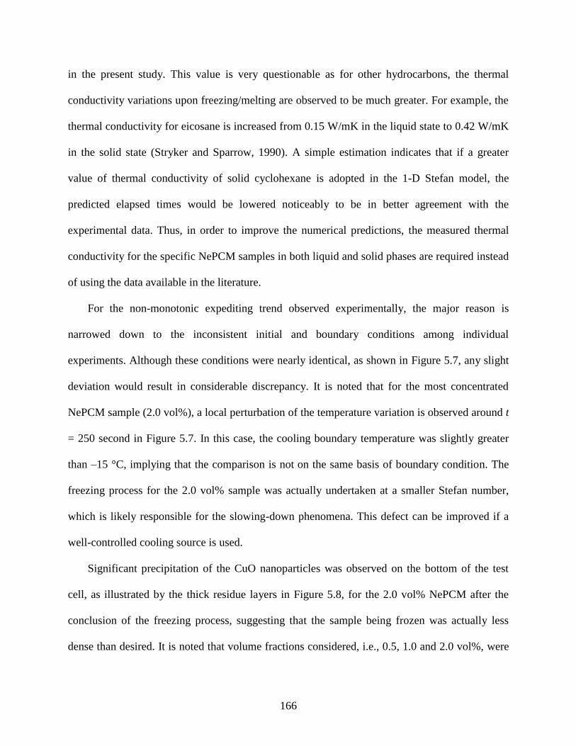
166
in the present study. This value is very questionable as for other hydrocarbons, the thermal
conductivity variations upon freezing/melting are observed to be much greater. For example, the
thermal conductivity for eicosane is increased from 0.15 W/mK in the liquid state to 0.42 W/mK
in the solid state (Stryker and Sparrow, 1990). A simple estimation indicates that if a greater
value of thermal conductivity of solid cyclohexane is adopted in the 1-D Stefan model, the
predicted elapsed times would be lowered noticeably to be in better agreement with the
experimental data. Thus, in order to improve the numerical predictions, the measured thermal
conductivity for the specific NePCM samples in both liquid and solid phases are required instead
of using the data available in the literature.
For the non-monotonic expediting trend observed experimentally, the major reason is
narrowed down to the inconsistent initial and boundary conditions among individual
experiments. Although these conditions were nearly identical, as shown in Figure 5.7, any slight
deviation would result in considerable discrepancy. It is noted that for the most concentrated
NePCM sample (2.0 vol%), a local perturbation of the temperature variation is observed around t
= 250 second in Figure 5.7. In this case, the cooling boundary temperature was slightly greater
than –15 °C, implying that the comparison is not on the same basis of boundary condition. The
freezing process for the 2.0 vol% sample was actually undertaken at a smaller Stefan number,
which is likely responsible for the slowing-down phenomena. This defect can be improved if a
well-controlled cooling source is used.
Significant precipitation of the CuO nanoparticles was observed on the bottom of the test
cell, as illustrated by the thick residue layers in Figure 5.8, for the 2.0 vol% NePCM after the
conclusion of the freezing process, suggesting that the sample being frozen was actually less
dense than desired. It is noted that volume fractions considered, i.e., 0.5, 1.0 and 2.0 vol%, were

167
relatively concentrated. Therefore, in order to attain a stabilized NePCM with desirable
expediting of freezing, a sample with relatively dilute concentration of nanoparticles is favored.
For individual combinations of base PCM and nanoparticles, the optimized value of loading of
nanoparticles may be found by performing a number of tests.
Furthermore, the establishment of the 1-D unidirectional freezing process was imperfect as
minor heat loss through the side walls of the test cell is unavoidable. Due to the surface tension
effect at the phase interface, non-planar, slightly concave downward freezing fronts were
observed during the freezing process. Additionally, pronounced void formation was also
observed in the solid layer upon freezing, as shown in Figure 5.9.
Discrepancy was also due to the neglected temperature dependence of the thermophysical
properties and effect of diffusion of nanoparticles in liquid. Such complexities of the freezing
experiment that were not addressed in the simple 1-D Stefan model led to other disagreements
between the experimental and numerical results.
5.3 Improved Experiment on NePCM Using a Copper Cold Plate (CCP)
5.3.1 Improvements relative to the previous work
Due to the pronounced discrepancies that were observed between the numerical predictions of
the 1-D Stefan model and the experimental data in the previous work, improvements were made in
order to address the aforementioned shortcomings. As discussed before, primary reasons for the
discrepancies were narrowed down to the mismatch of boundary conditions between the model and
experiment, lack of accurate thermal conductivity data, as well as significant precipitation for the

168
relatively heavy loading of nanoparticles. Therefore, the improvements on both experimental and
numerical sides relative to the previous work are outlined as follows:
1) An improved unidirectional freezing experimental setup was designed, in which a copper
cold plate was employed as the cooling source instead of using the TEC.
2) Cyclohexane-based NePCM samples with more dilute concentrations of CuO nanoparticles
were prepared and investigated.
3) The measured thermal conductivity of these cyclohexane-based NePCM samples, for both
liquid and solid phases, that has been documented in Chapter 3 was utilized in the
calculations of the 1-D Stefan model.
5.3.2 Experimental setup and procedure
As schematically shown in Figure 5.10, the experimental setup that has been used before
(Figure 5.1) was retained except for the cooling source, where the TEC was replaced with a copper
cold plate (CCP) that was operated with the aid of a constant-temperature bath/circulator. A
photograph of the CCP module (CP25G02, Lytron, Woburn, MA) with a mounting surface of 33
58 mm2 is shown in Figure 5.11, in which the internal channel consisting of criss-crossed fins is
displayed schematically by a cut-view inset (http://www.lytron.com/~/media/Images/Lytron/
Global/Standard%20Products/Pics/CP25/cold_plate_cp25.jpg).
Flow passageways of the CCP were connected to the inlet and outlet ports of a programmable
bath/circulator (TP-502P, Brookfield, Middleboro, MA) with a temperature stability of 0.01 °C and
with the pumping rate being adjustable (from 6 to 15 L/minute). It is noted that this circulator has
been used in Chapter 3 as the constant-temperature bath for controlling the temperature for thermal
conductivity measurements. A water/ethylene glycol 1:1 mixture with a freezing point of about –34

169
°C was used as the working fluid in order to attain bath temperature below ice point (0 °C). In
addition, a thick insulation box was fabricated to accommodate the CCP with all the surfaces being
protected except for a square opening that matches the size of the test cell left on the top surface.
Before mounting the test cell on the CCP, a thin layer of thermal grease was spread on the exposed
square surface of the CCP to reduce the contact resistance.
As presented before, the coordinates of the six (6) TCs mounted on the side wall of the test cell
are x1 = 1.6, x2 = 7.3, x3 = 12.6, x4 = 17.9, x5 = 23.6, and x6 = 29.3 mm (± 0.3 mm). Unlike the
previous setup, instead of mounting a TC on the top surface of the Al plate, the temperature at x0 = 0
mm was monitored by the TC#0 placed underneath the CCP for ease of installation. The
arrangement of the modified experimental setup is shown in Figure 5.12.
Cyclohexane was still chosen as the base PCM. In view of the dense samples (0, 0.5, 1.0 and
2.0 vol%, corresponding to 0, 3.8, 7.5 and 14.7 wt%, respectively) investigated before, four (4)
more dilute samples with 0, 1.0, 2.0 and 4.0 wt% of the CuO nanoparticles were prepared. A
volume of 20 mL was prepared for each of the samples. The experiments were still carried out in the
air-conditioned room that was maintained at about 25 °C. The boundary condition was, however,
different from the previous experimental setup, where the CCP was held at −5 °C for all the runs
performed. Comparing to the set point of the circulator, a typical temperature difference of only 1.5
°C was observed on the surface of the CCP by using a pumping rate of about 8 L/minute. This small
temperature difference was afforded by taking advantage of the extremely small thermal resistance
of the plate due to the pure copper design and the patented micro-channel structure inside the plate.
Therefore, in order to attain a constant plate temperature of −5 °C, the temperature of the circulator
was set at −6.5 °C. The stability of the plate temperature was observed to be of the same order of
170
that inside the circulator (± 0.03 °C). Additionally, the temperature data were still recorded at a
frequency of 0.2 Hz, i.e., every 5 seconds.
5.3.3 Results and discussion
Transient temperature variations recorded by TCs #0 to #3 for various NePCM samples during
the freezing process are presented in Figure 5.13. It took more than 4 hours to attain complete
freezing of the 32 mm thick samples and the freezing rate became much slower at later stages, as
indicated by the less steep temperature decaying rates at higher TC locations. Hence, only the data
up to 1 hour (3,600 second) for the four lowest TCs are shown in Figure 5.13. Comparing to the
significant time lag (about 20 minutes) of the cold boundary temperature associated with the TEC
adopted in the previous experimental setup, the CCP module being used was able to re-stabilize to
the set temperature within 20 second after loading the test cell. This favored feature is clearly
realized by the almost flat temperature variation of TC#0 that was mounted underneath the CCP
module. It is also shown that the plate temperatures were almost identical (−5.2 ± 0.05 °C) for
different runs, thus providing a consistent constant-temperature boundary condition. The freezing
rate is assessed by calculating the elapsed times to form a given thickness of solid layer, which was
determined by finding the intersections of the temperature curves with the flat line that represents
the constant freezing point (6.5 °C). Furthermore, the smooth variations around the phase change
region indicate that the supercooling for cyclohexane was negligible, unlike the significant
supercooling that was observed for experiments with distilled water. For ease of comparison, an
inset that presents the data of TC#2 (x = 7.3 mm) in the vicinity of the freezing point is given in
Figure 5.13.

171
In general, freezing was expedited as more nanoparticles were introduced and the greatest
expediting was achieved by introducing 2.0 wt% of nanoparticles. However, for the sample with the
highest concentration (4.0 wt%), freezing time was not further shortened relative to the 2.0 wt%
sample and was nearly recovered to that of the pure sample (0 wt%). Because the 4.0 wt% sample
exhibited desirable stability upon freeze/thaw cycling by visual observation, precipitation was
unlikely responsible for this anomalous slowing-down phenomenon. The possible reason will be
discussed below in regard to the measured thermal conductivity of the NePCM samples.
The measured elapsed times (up to 3,600 second) utilizing the original TEC setup and the
improved CCP setup are presented in Table 5.3. Comparison is made at various TC levels for the
case of pure cyclohexane. Since a lower boundary temperature was imposed in the experiments
adopting the TEC (T0 ≈ −15 °C), the elapsed times are clearly shown to have increased for the
improved experiments with the CCP module (T0 ≈ −5 °C). Comparison of the elapsed times for the
lowest TC (#1) in the test cell, however, exhibits the opposite trend due to the much shorter time lag
of the boundary temperature at the beginning afforded by the CCP module.
The elapsed times for the freezing front to reach the TC#2 at x = 7.3 mm were also predicted
numerically by employing the 1-D Stefan model presented in Chapter 4. The thermophysical
properties were estimated via the existing mixture models, except for thermal conductivity. As
presented in Chapter 3 (Figure 3.7), thermal conductivity values of the cyclohexane-based NePCM
samples measured at 10 °C were used for the liquid phase, whereas those measured at –5 °C were
adopted for the solid phase, as given in Table 5.4. Moreover, in the Stefan-model calculations, the
following parameters that are listed in Table 5.5 were specified to match the initial and boundary
conditions of the improved freezing experiment.

172
The experimentally-observed and the predicted elapsed times are presented in Table 5.6, in
which the relative percentages of expediting due to the presence of nanoparticles are given as well.
Note that because of the sampling rate of the DAQ unit (0.2 Hz), the resolution of the experimental
data was 5 s. Recalling the great discrepancies between experimental and numerical values observed
in the previous section for the TEC-based experimental setup, the present predictions were
significantly improved, due to the employment of the measured thermal conductivity data for the
solid phase and the stabilized boundary condition afforded by the CCP as well.
The experimentally-observed slowing-down phenomenon for the 4.0 wt% sample was verified
numerically, as the measured actual thermal conductivity was used in the predictions. It seems that
the enhancement of thermal conductivity was compromised when the loading of nanoparticles is
greater than 2.0 wt%. Both experimental and numerical results agree that the 2.0 wt% sample
resulted in the greatest percentage of expediting, which was 5.20% experimentally. In general, fairly
good agreement is exhibited with the numerical predictions being slightly under-estimated by about
18%, which was primarily due to deviation of the experimental setup from the 1-D Stefan model,
e.g., the imperfectly insulated walls.
5.4 Summary
A unidirectional freezing cell was designed to assure a thermally stable quasi 1-D freezing
process free of natural convection currents in such a way that the cell was cooled from below
with the side walls being insulted. TC readings at different heights along the freezing direction
were collected continuously, thus allowing determination of the progress of the freezing front.
An ice formation test was carried out to test the experimental setup with a TEC as the cooling
173
source. Natural convection associated with the density anomaly of water and significant
supercooling phenomena were successfully captured, thus indicating the applicability of the
experimental facilities.
As an example, cyclohexane-based NePCM samples were prepared and investigated by using
the TEC-driven experimental setup. Expedited freezing due to the presence of nanoparticles was
clearly observed. The time duration to form a 12.6 mm thick frozen layer was shown numerically
to be almost linearly shortened with increasing loading of nanoparticles. However, the
experimentally-observed expediting trend was not monotonic. The maximum percentage of
expediting was found to be 8.23% for the 0.5 vol% NePCM sample, whereas freezing was not
further expedited with increasing concentration. Moreover, at constant loading of nanoparticles,
pronounced discrepancies between the experimental and numerical results were observed. The
reasons for these discrepancies and routes to improve the current experimental investigation and
numerical predictions were discussed in relation to the mismatch between the experimental setup
and the physical model, lack of accurate data of thermophysical properties of NePCM, especially
in the solid phase and their dependence on temperature, as well as precipitation of nanoparticles
for the relatively concentrated samples studied.
In view of the aforementioned shortcomings, an improved experimental study was conducted
for more dilute NePCM samples. Better control of the cold boundary temperature was achieved by
utilizing a CCP with the aid of a programmable circulator instead of using the TEC. The quality of
the experimental data was thus improved. It was shown that freezing was expedited as more
nanoparticles were introduced and the trend was still not monotonic. The 2.0 wt% sample yielded
the highest percentage of expediting (5.20%), whereas freezing was slightly slowed down when the
loading of nanoparticles was further increased to 4 wt%. This was related to the non-monotonic

174
enhancement of thermal conductivity in the solid phase. Instead of adopting the questionable
thermal conductivity value available in the literature, better numerical predictions were obtained by
employing the in-house measured thermal conductivity data. Fairly good agreement between the
experimental and numerical results was exhibited with the numerical predictions being slightly
under-estimated. Upon eliminating the major shortcomings, the remaining sources for discrepancies
between the experimental and numerical results seemed to be primarily attributed to the inherent
deviation of the experimental setup from the physical model due to imperfect thermal insulation.
Other complexities associated with the freezing experiment, e.g., non-planar freezing front, void
formation in solid phase upon freezing, and diffusion and precipitation of nanoparticles in liquid,
which were not accounted for in the simple model, could be other major contributors to the
disagreements.

175
Table 5.1 The experimental parameters of the TEC setup imposed for the 1-D Stefan
problem
Parameter Quantity
s 12.6 mm
Tf 6.5 °C
Ti 25.5 °C
T0 −15 °C

176
Table 5.2 Comparison of the experimental and numerical results of the elapsed times for the
freezing front to reach the height of 12.6 mm
Volume fraction
(vol%)
Mass fraction
(wt%)
Experimental data Numerical predictions
Time (s) Expediting Time (s) Expediting
0.0 0.0 1,215 — 2,240 —
0.5 3.8 1,115 8.23% 2,228 0.54%
1.0 7.5 1,175 3.29% 2,216 1.07%
2.0 14.7 1,245 −2.47% 2,193 2.10%

177
Table 5.3 Comparison of the measured elapsed freezing times (unit: second) for the frozen
layer to reach various TC levels utilizing the original TEC and the improved CCP setups for pure
cyclohexane
TC number TEC setup CCP setup
#1 115 95
#2 545 865
#3 1,215 1,920
#4 2,115 > 3,600
#5 > 3,600 —
#6 — —

178
Table 5.4 Adopted thermal conductivity (unit: W/mK) from measurements of both liquid
and solid cyclohexane-based NePCM samples with various loadings of nanoparticles
Mass fraction (wt%) Liquid (10 °C) Solid (–5 °C)
0 0.1225 0.2689
1 0.1231 0.2764
2 0.1238 0.2865
4 0.1243 0.2716

179
Table 5.5 The experimental parameters for the improved experimental setup using a CCP
utilized for the 1-D Stefan problem
Parameter Quantity
s 7.3 mm
Tf 6.5 °C
Ti 25 °C
T0 −5.2 °C

180
Table 5.6 Comparison between the observed and predicted elapsed times to form a 7.3 mm
thick frozen layer of NePCM
Mass fraction (wt%)
Experimental data Numerical predictions
Time (s) Expediting Time (s) Expediting
0 865 — 708.3 —
1 835 3.47% 679.5 4.07%
2 820 5.20% 651.0 8.09%
4 860 0.58% 696.6 1.65%

181
Figure 5.1 Schematic diagrams of (a) the unidirectional freezing experimental setup with a thermoelectric cooler (TEC) and (b)
the arrangement of the thermocouples

182
Figure 5.2 Photograph of the arrangement of the unidirectional freezing experimental setup
operated with a thermoelectric cooler (TEC)
DAQ
Power supply
Fan guide cone
Insulation
Test cell
Air flow

183
Figure 5.3 Photograph of a close-up view of the transparent test cell filled with distilled
water prior to an ice formation experiment
Heat sink
TEC
Insulation Test cell

184
Figure 5.4 Comparison of transient variations of the temperature at various locations during the ice formation process

185
Figure 5.5 Density of water (ice) as a function of temperature

186
Figure 5.6 A sequence of photographs displaying the unidirectional ice formation process
within the test cell with the ice/water interface identified by dashed lines

187
Figure 5.7 Comparison of transient variations of the temperature at various locations: x0 = 0 (TC#0), x1 = 1.6 (TC#1), x2 = 7.3
(TC#2), x3 = 12.6 (TC#3) and x4 = 17.9 mm (TC#4) for the TEC setup

188
Figure 5.8 Photographs of (a) the top and (b) side views of the test cell with the most
concentrated cyclohexane-based NePCM sample (2.0 vol%) after the freezing experiment,
showing significant precipitation of CuO nanoparticles on the bottom

189
Figure 5.9 Photographs of (a) the side view of the test cell showing worm-like slender voids
formed in the frozen pure cyclohexane and (b) top view of a frozen cyclohexane-based NePCM
sample (2.0 vol%) with the holes indicating the formed voids of various sizes
24.8 mm

190
Figure 5.10 Schematic diagrams of (a) the unidirectional freezing experimental setup with a CCP and (b) the arrangement of the
thermocouples
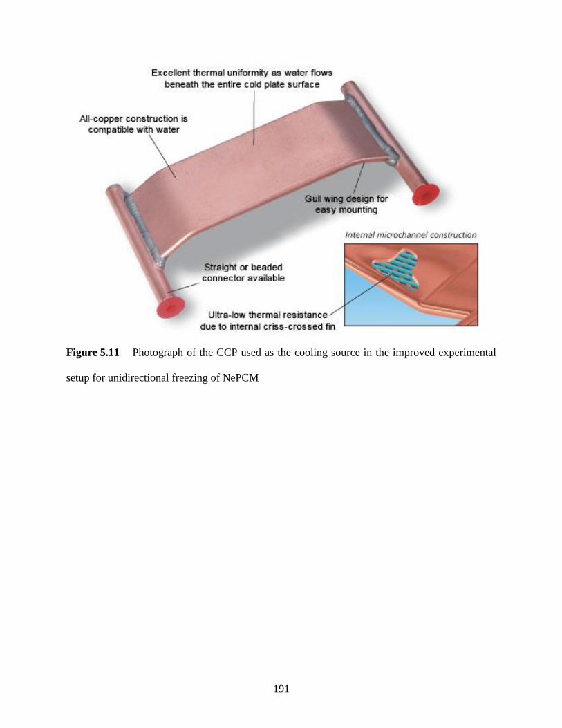
191
Figure 5.11 Photograph of the CCP used as the cooling source in the improved experimental
setup for unidirectional freezing of NePCM

192
Figure 5.12 Photograph of the arrangement of the improved unidirectional freezing
experimental setup with a CCP
DAQ
Constant-temperature bath/Circulator
CCP
Insulation
Test cell

193
Figure 5.13 Comparison of transient variations of the local temperature at various locations: x0 = 0 (TC#0), x1 = 1.6 (TC#1), x2 =
7.3 (TC#2) and x3 = 12.6 mm (TC#3) for the CCP setup

194
Chapter 6 Conclusions and Perspectives
In this chapter, remarks are drawn to conclude this dissertation. Open questions, perspectives
and suggested future work with regard to fundamental research and applications of NePCM are
also discussed.
6.1 Concluding Remarks
Based on the experimental and numerical results presented in the previous Chapters,
concluding remarks are drawn as follows:
a) Hydrocarbon-based NePCM samples were prepared with sodium-oleate-stabilized CuO
nanoparticles. Desirable stability of the samples upon freeze/thaw cycling was visually
observed for relatively dilute concentrations. Nearly no precipitation was observed for the
cyclohexane-based NePCM samples with mass fractions up to 4 percent.
b) Enhanced thermal conductivity of both cyclohexane- and eicosane-based NePCM was
clearly achieved by introducing the relatively more conductive CuO nanoparticles. The
TPS technique was successfully used for measuring thermal conductivity of the NePCM
samples in both solid and liquid phases.
c) In the range of the loading of nanoparticles studied (mass fraction less than 10 percent),
the relative monotonic enhancement of thermal conductivity in liquid phase was in good
agreement with the predictions of the Maxwell’s equation. Considering the solid phase,

195
however, a non-monotonic phenomenon was exhibited when the mass fraction was
greater than 2 percent.
d) Temperature dependence of the thermal conductivity of NePCM was shown to be similar
to that for the corresponding base PCM. In the liquid phase, the enhancement was slightly
more marked with increasing temperature, probably due to more intensive diffusion of
nanoparticles at high temperatures.
e) For the base PCM with considerable supercooling, i.e., eicosane, the measured thermal
conductivity was significantly dependent on the formation of the solid samples. Close
attention should be paid to preparation of the samples so as to satisfy the requirement of
the TPS technique.
f) A simple 1-D, two-region Stefan problem was formulated to describe the unidirectional
freezing of NePCM under the single-phase assumption. The problem was successfully
solved by employing both a combined analytic/integral approach and the extended LBM
with enthalpy formulation.
g) Due to the enhanced thermal conductivity, expedited unidirectional freezing of both
aqueous and cyclohexane-based NePCM with various nanoparticles was shown
numerically through the 1-D Stefan model. The extent of expediting was observed to be
linearly increased as more nanoparticles were introduced.
h) A quasi 1-D unidirectional freezing test cell was designed, constructed and tested. The
test cell was cooled from the bottom to eliminate natural convection upon freezing. Both
visualized observation and indirect determination of the evolution of the freezing front
were enabled in this setup.

196
i) Unidirectional freezing of cyclohexane-based NePCM was first performed with the
original setup with a TEC being used as the cooling source. Due to the lack of
temperature control of the TEC, pronounced discrepancies between the experimental data
and the numerical predictions of the 1-D Stefan model were observed.
j) The experimental setup was then improved by replacing the TEC with a CCP with the aid
of a controllable circulator. Also owing to adoption of the measured thermal conductivity
of the NePCM samples, the experimental results exhibited good agreement with the
numerical predictions.
k) The refined experimental results showed that the expediting of unidirectional freezing
was not monotonic with increasing loading of nanoparticles, which was confirmed by a
similar effect in measurements of the solid phase thermal conductivity. The maximum
extent of expediting of 5.2 percent was achieved for the 2 percent sample.
In conclusion, the observed thermal conductivity enhancement and expediting of
unidirectional freezing of hydrocarbon-based NePCM samples justify the great potential of such
materials in the applications of latent heat-driven thermal energy storage.
6.2 Suggestions for Future Work
Although the NePCM have been shown to be a promising solution for improved thermal
energy storage, the studies in this dissertation were meant to open the door for research of such
emerging materials. The future work is suggested to be focused on the following aspects:

197
a) To improve the colloidal stability will always be the most challenging goal. Engineers
should work closely with chemists to find ways to prepare NePCM colloids with
desirable stability.
b) Not limited to hydrocarbons, NePCM with other base PCM, e.g., water and molten salts
for different ranges of working temperature, should be prepared and characterized in
order to build a property database for real-world applications. A variety of nano-
structured materials should also be attempted, especially those possessing extremely high
thermal conductivity, e.g., silver nanoparticles, and carbon nanotubes, etc.
c) The trade-off between the increased viscosity, which suppresses natural convection, and
the enhanced thermal conductivity, which augments heat conduction, of melting heat
transfer of NePCM is of great interest.
d) Another trade-off between the expedited energy charging/discharging rate afforded by the
enhanced thermal conductivity and the lowered energy storage density due to decreased
specific heat capacity and latent heat is of importance for real-world applications.
e) To consider the diffusion of nanoparticles in the mathematical modeling of phase change
heat transfer of NePCM is challenging and will provide a better understanding of the
mechanisms of heat transfer enhancement due to the presence of nanoparticles.
f) Advanced experimental techniques, e.g., the small-angle X-ray (SAXS) and neutron
scatterings (SANS), may be used for studying the dynamics of freezing/thawing of
NePCM with emphasis on characterizing the interactions of the nanoparticles with the
moving phase interface.
In summary, greater effort must be directed to both fundamental and applied investigations of
NePCM with the aid of advanced experimental and numerical techniques.

198
Bibliography
Abhat, A., 1976, ―Experimental Investigation and Analysis of a Honeycomb-Packed Phase
Change Material Device,‖ Paper No. AIAA-76-437, AIAA 11th Thermophysics Conference,
San Diego, CA.
Abhat, A., Aboul-Enein, S., and Malatidis, N. A., 1981, ―Heat-of-Fusion Storage Systems for
Solar Heating Applications,‖ Proceedings of an International TNO-Symposium, Martinus
Nijhoff Publishers, Amsterdam, The Netherlands, pp. 157-171.
Abhat, A., 1983, ―Low Temperature Latent Heat Thermal Energy Storage: Heat Storage
Materials,‖ Solar Energy, 30(4), pp. 313-332.
Agyenim, F., Eames, P., and Smyth, M., 2009, ―A Comparison of Heat Transfer Enhancement in
a Medium Temperature Thermal Energy Storage Heat Exchanger Using Fins,‖ Solar Energy,
83(9), pp. 1509-1520.
Batchelor, G. K., 1974, ―Transport Properties of Two-Phase Materials with Random Structure,‖
Annual Review of Fluid Mechanics, 6, pp. 227-255.
Bentilla, E. W., Sterrett, K. F., and Karre, L. E., 1966, ―Research and Development Study on
Thermal Control by Use of Fusible Materials,‖ Northrop Space Laboratories Interim Report
No. NSL-65-16-1, NASA Marshall Space Flight Center, Huntsville, AL.
Brent, A. D., Voller, V. R., and Reid, K. J., 1988, ―Enthalpy-Porosity Technique for Modeling
Convection-Diffusion Phase Change: Application to the Melting of a Pure Metal,‖ Numerical
Heat Transfer, Part A: Applications, 13(3), pp. 297-318.

199
Boger, D. V., and Westwater, J. W., 1967, ―Effect of Buoyancy on the Melting and Freezing
Process,‖ Journal of Heat Transfer, 89(1), pp. 81-89.
Bugaje, I. M., 1997, ―Enhancing the Thermal Response of Latent Heat Storage System,‖
International Journal of Energy Research, 21(9), pp. 759-766.
Buongiorno, J., et al., 2009, ―A Benchmark Study on the Thermal Conductivity of Nanofluids,‖
Journal of Applied Physics, 106(9), 094312.
Cabeza, L. F., Mehling, H., Hiebler, S., and Ziegler, F., 2002, ―Heat Transfer Enhancement in
Water when Used as PCM in Thermal Energy Storage,‖ Applied Thermal Engineering,
22(10) pp. 1141-1151.
Cesari, F., 1992, ―An Enthalpy Formulation of the Conduction Problem with Phase Changes,‖
Computers & Structures, 44(5), pp. 983-987.
Chalmers, B., 1959, ―How Water Freezes,‖ Scientific American, 200(2), pp. 114-122.
Chatterjee, D., and Chakraborty, S., 2005, ―An Enthalpy-Based Lattice Boltzmann Model for
Diffusion Dominated Solid-Liquid Phase Transformation,‖ Physics Letters A, 341(1-4), pp.
320-330.
Chen, S., and Doolen, G. D., 1998, ―Lattice Boltzmann Method for Fluid Flows,‖ Annual Review
of Fluid Mechanics, 30, pp. 329-364.
Chen, Y., Ohashi, H., and Akiyama, M., 1995, ―Heat Transfer in Lattice BGK Modeled Fluid,‖
Journal of Statistical Physics, 81(1-2), pp. 71-85.
Cho, S. H., and Sunderland, J. E., 1969, ―Heat-Conduction Problems with Melting or Freezing,‖
Journal of Heat Transfer, 91(3), pp. 421-426.
Chow, L. C., Zhong, J. K., and Beam, J. E., 1996, ―Thermal Conductivity Enhancement for
Phase Change Storage Media,‖ International Communications in Heat and Mass Transfer,

200
23(1), pp. 91-100.
Clary, D. R., and Mills, G., 2010, private communication.
Clary, D. R., and Mills, G., 2011, ―Preparation and Thermal Properties of CuO Particles‖,
Journal of Physical Chemistry C, 115(5), pp. 1767-1775.
Coleman, H. W., and Steele, Jr., W. G., 1989, Experimentation and Uncertainty Analysis for
Engineers, John Wiley & Sons, Inc., New York, NY.
Cui, Y., Liu, C., Hu, S., and Yu, X., 2011, ―The Experimental Exploration of Carbon Nanofiber
and Carbon Nanotube additives on Thermal Behavior of Phase Change Materials,‖ Solar
Energy Materials and Solar Cells, 95(4), pp. 1208-1212.
Das, S. K., Choi, S. U. S., Yu, W., and Pradeep, R., 2008, Nanofluids: Science and Technology,
John Wiley & Sons, Inc., Hoboken, NJ.
De Jong, A. G., and Hoogendoorn, C. J., 1981, ―Improvement of Heat Transport in Paraffins for
Latent Heat Storage Systems,‖ Proceedings of an International TNO-Symposium, Martinus
Nijhoff Publishers, Amsterdam, The Netherlands, pp. 123-133.
Eftekhar, J., Haji-Sheikh, A., and Lou, D. Y. S., 1984, ―Heat Transfer Enhancement in a Paraffin
Wax Thermal Storage System,‖ Journal of Solar Energy Engineering, 106(3), pp. 299-306.
Elgafy, A., and Lafdi, K., 2005, ―Effect of Carbon Nanofiber Additives on Thermal Behavior of
Phase Change Materials,‖ Carbon, 43(15), pp. 3067-3074.
Ettouney, H. M., Alatiqi, I., Al-Sahali, M., and Al-Ali, S. A., 2004, ―Heat Transfer Enhancement
by Metal Screens and Metal Spheres in Phase Change Energy Storage Systems,‖ Renewable
Energy, 29(6), pp. 841-860.
Ettouney, H. I., Alatiqi, M., Al-Sahali, M., and Al-Hajirie, K., 2006, ―Heat Transfer
Enhancement in Energy Storage in Spherical Capsules Filled with Paraffin Wax and Metal

201
Beads,‖ Energy Conversion and Management, 47(2), pp. 211-228.
Evans, W., Prasher, R., Fish, J., Meakin, P., Phelan, and Keblinski, P., 2008, ―Effect of
Aggregation and Interfacial Thermal Resistance on Thermal Conductivity of
Nanocomposites and Colloidal Nanofluids,‖ International Journal of Heat and Mass
Transfer, 51(5-6), pp. 1431-1438.
Fan, L., and Khodadadi, J. M., 2011, ―Thermal Conductivity Enhancement of Phase Change
Materials for Thermal Energy Storage: A Review,‖ Renewable and Sustainable Energy
Reviews, 15(1), pp. 24-46.
Farid, M. M., Khudhair, A. M., Razack, S. A. K., and Al-Hallaj, S., 2004, ―A Review on Phase
Change Energy Storage: Materials and Applications,‖ Energy Conversion and Management,
45(9-10), pp. 1597-1615.
Fluent Inc., 2006, Fluent 6.3 User’s Guide, Fluent Inc., Lebanon, NH.
Fukai, J., Oishi, A., Kodama, Y., Kanou, M., and Miyatake, O., 1999, ―Improvement of
Discharge Characteristics of Latent Heat Thermal Storage Unit by Using Carbon Fibers,‖
Paper No. AJTE99-6338, Proceedings of the 5th ASME/JSME Joint Thermal Engineering
Conference, San Diego, CA.
Fukai, J., Kanou, M., Kodama, Y., and Miyatake, O., 2000, ―Thermal Conductivity
Enhancement of Energy Storage Media Using Carbon Fibers,‖ Energy Conversion and
Management, 41(14), pp. 1543-1556.
Griggs, E. I., Pitts, D. R., and Humphries, W. R., 1974, ―Transient Analysis of a Thermal
Storage Unit Involving a Phase Change Material,‖ Paper No. 74-WA/HT-21, ASME Winter
Annual Meeting, New York, NY.
Günther, E., Mehling, H., and Hiebler, S., 2007, ―Modeling of Subcooling and Solidification of

202
Phase Change Materials,‖ Modelling and Simulation in Materials Science and Engineering,
15(8), pp. 879-892.
Gupta, S. C., 2003, The Classical Stefan Problem, Elsevier Science, Amsterdam, The
Netherlands.
Gustafsson, S. E., 1991, ―Transient Plane Source Technique for Thermal Conductivity and Thermal
Diffusivity Measurements of Solid Materials,‖ Review of Scientific Instruments, 62(3), pp 797-
804.
Gustavsson, M., Karawacki, E., and Gustafsson, S. E., 1994, ―Thermal Conductivity, Thermal
Diffusivity, and Specific Heat of Thin Samples from Transient Measurements with Hot Disk
Sensors,‖ Review of Scientific Instruments, 65(12), pp 3856-3859.
Haji-Sheikh, A., Eftekhar, J., and Lou, D. Y. S., 1983, ―Some Thermophysical Properties of
Paraffin Wax as a Thermal Storage Medium,‖ Progress in Astronautics and Aeronautics,
AIAA, New York, NY, 86, pp. 241-253.
Hale, D. V., Hoover, M. J., and O’Neill, M. J., 1971, ―Phase Change Materials Handbook,‖
NASA Contractor Report No. NASA CR-61363, Huntsville Research and Engineering
Center, Lockheed Missiles and Space Company, Inc., Huntsville, AL.
Hammerschlag, R., and Schaber, C. P., 2008, ―Energy Storage Technologies,‖ in Energy
Conversion, edited by Goswami, D. Y., and Kreith, F., CRC Press, Boca Raton, FL, p. 15-5.
Hasnain, S. M., 1998, ―Review on Sustainable Thermal Energy Storage Technologies, Part I:
Heat Storage Materials and Techniques,‖ Energy Conversion and Management, 39(11), pp.
1127-1138.
Hasselman, D. P. H., and Johnson, L. F., 1987, ―Effective Thermal Conductivity of Composites
with Interfacial Thermal Barrier Resistance,‖ Journal of Composite Materials, 21(6), pp.

203
508-515.
Heimenz, P. C., and Rajagopalan, R., 1997, Principles of Colloid and Surface Chemistry, Marcel
Dekker, Inc., New York, NY.
Henze, H. R., and Humphrey, J. A. C., 1981, ―Enhanced Heat Conduction in Phase-Change
Thermal Energy Storage Devices,‖ International Journal of Heat and Mass Transfer, 24(3),
pp. 459-474.
Ho, C. J., and Gao, J. Y., 2009, ―Preparation and Thermophysical Properties of Nanoparticle-in-
Paraffin Emulsion as Phase Change Material,‖ International Communications in Heat and
Mass Transfer, 36(15), pp. 467-470.
Holman, J. P., 1994, Experimental Methods for Engineers, McGraw-Hill, Inc., New York, NY,
pp. 371-373.
Hoover, M. J., Grodzka, P. G., and O’Neill, M. J., 1971, ―Space Thermal Control Development,‖
Final Report No. LMSC-HREC D225500, Huntsville Research and Engineering Center,
Lockheed Missiles and Space Company, Inc., Huntsville, AL.
Hou, S., Zou, Q., Chen, S., Doolen, G., and Cogley, A. C., 1995, ―Simulation of Cavity Flow by
the Lattice Boltzmann Method,‖ Journal of Computational Physics, 118(2), pp. 329-347.
Huber, C., Parmigiani, A., Chopard, B., Manga, M., and Bachmann, O., 2008, ―Lattice
Boltzmann Model for Melting with Natural Convection,‖ International Journal of Heat and
Fluid Flow, 29(5), pp. 1469-1480.
Humphries, W. R., 1974, ―Performance of Finned Thermal Capacitors,‖ NASA Technical Note
No. D-7690.
Humphries, W. R., and Griggs, E. I., 1977, ―A Design Handbook for Phase Change Thermal
Control and Energy Storage Devices,‖ NASA Technical Paper No. 1074.

204
Incropera, F. P., DeWitt, D. P., Bergman, T. L., and Lavine, A. S., 2007, Fundamentals of Heat
and Mass Transfer, John Wiley & Sons, Inc., Hoboken, NJ, pp. 259-261.
Jang, S. P., and Choi, S. U. S., 2007, ―Effects of Various Parameters on Nanofluid Thermal
Conductivity,‖ Journal of Heat Transfer, 129(5), pp. 617-623.
Jegadheeswaran, S., and Pohekar, S. D., 2009, ―Performance Enhancement in Latent Heat
Thermal Storage System: A Review,‖ Renewable and Sustainable Energy Reviews, 13(9),
pp. 2225-2244.
Jiaung, W.-S., Ho, J.-R., and Kuo, C.-P., 2001, ―Lattice Boltzmann Method for the Heat
Conduction Problem with Phase Change,‖ Numerical Heat Transfer, Part B: Fundamentals,
39(2): 167-187.
Jiji, L. M., 2009, Heat Conduction, Springer, Berlin, Germany, pp. 186-188.
Kamimoto, M., 1987, ―Thermal Energy Storage Technology,‖ International Journal of Solar
Energy, 5(1), pp. 21-33.
Kenisarin, M., and Mahkamov, K., 2007, ―Solar Energy Storage using Phase Change Materials,‖
Renewable and Sustainable Energy Reviews, 11(9), pp. 1913-1965.
Khodadadi, J. M., 2011, private communication.
Khodadadi, J. M., and Hosseinizadeh, S. F., 2007, ―Nanoparticle-Enhanced Phase Change
Materials (NEPCM) with Great Potential for Improved Thermal Energy Storage,‖
International Communications in Heat and Mass Transfer, 34(5), pp. 534-543.
Knowles, T. R., and Webb, G. W., 1987, ―M/PCM Composite Thermal Storage Materials,‖
Paper No. AIAA-87-1489, AIAA 22nd Thermophysics Conference, Honolulu, HI.
Koizumi, H., 2004, ―Time and Spatial Heat Transfer Performance around an Isothermally Heated
Sphere Placed in a Uniform, Downwardly Directed Flow (in Relation to the Enhancement of
205
Latent Heat Storage Rate in a Spherical Capsule),‖ Applied Thermal Engineering, 24(17-18)
pp. 2583-2600.
Koo, J, and Kleinstreuer, 2004, ―A New Thermal Conductivity Model for Nanofluids,‖ Journal
of Nanoparticle Research, 6(6), pp. 577-588.
Koo, J, and Kleinstreuer, 2005, ―Impact Analysis of Nanoparticle Motion Mechanisms on the
Thermal Conductivity of Nanofluids,‖ International Communications in Heat and Mass
Transfer, 32(9), pp. 1111-1118.
Liu, Y.-D., Zhou, Y.-G., Tong, M.-W., and Zhou, X.-S., 2009, ―Experimental Study of Thermal
Conductivity and Phase Change Performance of Nanofluids PCMs,‖ Microfluidics and
Nanofluidics, 7(4), pp. 579-584.
Maxwell, J. C., 1873, A Treatise on Electricity and Magnetism, Clarendon Press, Oxford, UK.
Mehling, H., and Cabeza, L. F., 2007, ―Phase Change Materials and Their Basic Properties,‖ in
Thermal Energy Storage for Sustainable Energy Consumption, edited by Paksoy, H. A.,
Springer, Berlin, Germany, p. 262.
Mesalhy, O., Lafdi, K., Elgafy, A., and Bowman, K., 2005, ―Numerical Study for Enhancing the
Thermal Conductivity of Phase Change Material (PCM) Storage Using High Thermal
Conductivity Porous Matrix,‖ Energy Conversion and Management, 46(6), pp. 847-867.
Mettawee, E.-B. S., and Assassa, G. M. R., 2007, ―Thermal Conductivity Enhancement in a
Latent Heat Storage System,‖ Solar Energy, 81(7), pp. 839-845.
Nakaso, K., Teshima, H., Yoshimura, A., Nogami, S., Hamada, Y., and Fukai, J., 2008,
―Extension of Heat Transfer Area using Carbon Fiber Cloths in Latent Heat Thermal Energy
Storage Tanks,‖ Chemical Engineering and Processing, 47(5), pp. 879-885.
Nan, C.-W., Birringer, R., Clarke, D. R., and Gleiter, H., 1997, ―Effective Thermal Conductivity
206
of Particulate Composites with Interfacial Thermal Resistance,‖ Journal of Applied Physics,
81(10), pp. 6692-6699.
Nayak, K. C., Saha, S. K., Srinivasan, K., and Dutta, P., 2006, ―A Numerical Model for Heat
Sinks with Phase Change Materials and Thermal Conductivity Enhancers,‖ International
Journal of Heat and Mass Transfer, 49(11-12), pp. 1833-1844.
Nomura S., and Chou, T.-W., 1980, ―Bounds of Effective Thermal Conductivity of Short-Fiber
Composites,‖ Journal of Composite Materials, 14(2), pp. 120-129.
Özışık, M. N., 1980, Heat Conduction, John Wiley & Sons, Inc., New York, NY.
Pal, D., and Joshi, Y. K., 1998, ―Thermal Management of an Avionics Module Using Solid-
Liquid Phase-Change Materials,‖ Journal of Thermophysics and Heat Transfer, 12(2), pp.
256-262.
Progelhof, R. C., Throne, J. L., and Ruetsch, R. R., 1976, ―Methods for Predicting the Thermal
Conductivity of Composite Systems: A Review,‖ Polymer Engineering and Science, 16(9),
pp. 615-625.
Quarteroni, A., Sacco, R., and Saleri, F., 2007, Numerical Mathematics, Springer, Berlin,
Germany.
Ramires, M. L. V., Nieto de Castro, C. A., Nagasaka, Y., Nagashima, A., Assael, M. J., and
Wakeham, W. A., 1995, ―Standard Reference Data for the Thermal Conductivity of Water,‖
Journal of Physical and Chemical Data, 24(3), pp. 1377-1381.
Rastorguev, Yu. L., Bogatov, G. F., and Grigor’ev, B. A., 1974, ―Thermal Conductivity of Higher
n-Alkanes,‖ Chemistry and Technology of Fuels and Oils, 10(9), pp 728-732.
Regin, A. F., Solanki, S. C., and Saini, J. S., 2008, ―Heat Transfer Characteristics of Thermal
Energy Storage System using PCM Capsules: A Review,‖ Renewable and Sustainable

207
Energy Reviews, 12(9), pp. 2438-2458.
Seeniraj, R. V., Velraj, R., and Narasimhan, N. L., 2002, ―Heat Transfer Enhancement Study of a
LHTS Unit Containing Dispersed High Conductivity Particles,‖ Journal of Solar Energy
Engineering, 124(7), pp. 243-249.
Shaikh, S., Lafdi, K., and Hallinan, K., 2008, ―Carbon Nanoadditives to Enhance Latent Energy
Storage of Phase Change Materials,‖ Journal of Applied Physics, 103(9), pp. 094302.
Sharma, S. D., and Sagara, K., 2005, ―Latent Heat Storage Materials and Systems: A Review,‖
International Journal of Green Energy, 2(1), pp. 1-56.
Shyy, W., Udaykumar, H. S., Rao, M. M., and Smith, R. W., 1996, Computational Fluid
Dynamics with Moving Boundaries, Taylor & Francis, Philadelphia, PA.
Siegel, R., 1977, ―Solidification of Low Conductivity Material Containing Dispersed High
Conductivity Particles,‖ International Journal of Heat and Mass Transfer, 20(10), pp. 1087-
1089.
Stritih, U., 2004, ―An Experimental Study of Enhanced Heat Transfer in Rectangular PCM
Thermal Storage,‖ International Journal of Heat and Mass Transfer, 47(12-13), pp. 2841-
2847.
Stryker, P. C., and Sparrow, E. M., 1990, ―Application of a Spherical Thermal Conductivity Cell
to Solid n-Eicosane Paraffin,‖ International Journal of Heat and Mass Transfer, 33(9), pp.
1781-1793.
Succi, S., 2001, The Lattice Boltzmann Equation for Fluid Dynamics and Beyond, Oxford
University Press, Oxford, UK.
Sulfredge, C. D., Chow, L. C., and Tagavi, K. A., 1993, ―Void Initiation and Growth in
Unidirectional Freezing: the Influence of Natural Convection,‖ Experimental Heat Transfer,

208
6(4), pp. 411-436.
Tan, F. L., Hosseinizadeh, S. F., Khodadadi, J. M., and Fan, L., 2009, ―Experimental and
Computational Study of Constrained Melting of Phase Change Materials (PCM) inside a
Spherical Capsule,‖ International Journal of Heat and Mass Transfer, 52(15-16), pp. 3464-
3472.
Tarzia, D. A., 2000, ―A Bibliography on Moving-Free Boundary Problems for the Heat-
Diffusion Equation. The Stefan and Related Problems,‖ MAT, Series A, No. 2, 297 pages.
Tong, X., Khan, J. A., and Amin, M. R., 1996, ―Enhancement of Heat Transfer by Inserting a
Metal Matrix into a Phase Change Material,‖ Numerical Heat Transfer, Part A: Applications,
30(2), pp. 125-141.
Velraj, R., Seeniraj, R. V., Hafner, B., Faber, C., and Schwarzer, K., 1999, ―Heat Transfer
Enhancement in a Latent Heat Storage System,‖ Solar Energy, 65(3), pp. 171-180.
Wang, J., Xie, H., and Xin, Z., 2008, ―Thermal Properties of Heat Storage Composites
Containing Multiwalled Carbon Nanotubes,‖ Journal of Applied Physics, 104(11), pp.
113537.
Wang, J., Xie, H., and Xin, Z., 2009, ―Thermal Properties of Paraffin Based Composites
Containing Multi-Walled Carbon Nanotubes,‖ Thermochimica Acta, 488(1-2), pp. 39-42.
Wang, J., Xie, H., Li, Y., and Xin, Z., 2010a, ―PW Based Phase Change Nanocomposites
Containing γ-Al2O3,‖ Journal of Thermal Analysis and Calorimetry, 102(2), pp. 709-713.
Wang, J., Xie, H., Xin, Z., Li, Y., and Chen, L., 2010b, ―Enhancing Thermal Conductivity of
Palmitic Acid Based Phase Change Materials with Carbon Nanotubes as Fillers,‖ Solar
Energy, 84(2), pp. 339-344.
Wang, J., Xie, H., Xin, Z., and Li, Y., 2010c, ―Increasing the Thermal Conductivity of Palmitic

209
Acid by the Addition of Carbon Nanotubes,‖ Carbon, 48(14), pp. 3979-3986.
Wang, N., Yang, S., Zhu, D., and Ju, X., 2010d, ―Preparation and Heat Transfer Behavior of
Paraffin based Composites Containing Nano-Copper Particles,‖ Paper No. P3.81,
Proceedings of the 7th International Conference on Multiphase Flow, Tampa, FL.
Watanabe, H., and Kato, H., 2004, ―Thermal Conductivity and Thermal Diffusivity of Twenty-
Nine Liquids: Alkenes, Cyclic (Alkanes, Alkenes, Alkadienes, Aromatics), and Deuterated
Hydrocarbons,‖ Journal of Chemical and Engineering Data, 49(4), pp. 809-825.
White, R. E., 1982, ―An Enthalpy Formulation of the Stefan Problem,‖ SIAM Journal on
Numerical Analysis, 19(6), pp. 1129-1157.
Wolf-Gradrow, D. A., 2000, Lattice Gas-Cellular Automata and Lattice Boltzmann Models,
Springer-Verlag, Berlin, Germany.
Wu, S., Zhu, D., Li, X., Li, H., and Lei, J., 2009, ―Thermal Energy Storage Behavior of Al2O3-
H2O Nanofluids,‖ Thermochimica Acta, 483(1-2), pp. 73-77.
Wu, S., Zhu, D., Zhang, X., and Huang, J., 2010, ―Preparation and Melting/Freezing
Characteristics of Cu/Paraffin Nanofluid as Phase-Change Material (PCM),‖ Energy and
Fuels, 24(3), pp. 1894-1898.
Yu, W., France, D. M., Routbort, J. L., and Choi, S. U. S., 2008, ―Review and Comparison of
Nanofluid Thermal Conductivity and Heat Transfer Enhancements,‖ Heat Transfer
Engineering, 29(5), pp. 432-460.
Zalba, B., Marin, J. M., Cabeza, L. F., and Mehling, H., 2003, ―Review on Thermal Energy
Storage with Phase Change: Materials, Heat Transfer Analysis and Applications,‖ Applied
Thermal Engineering, 23(3) pp. 251-283.
Zeng, J. L., Sun, L. X., Xu, F., Tan, Z. C., Zhang, Z. H., Zhang, J., and Zhang, T., 2007, ―Study

210
of a PCM Based Energy Storage System Containing Ag Nanoparticles,‖ Journal of Thermal
Analysis and Calorimetry, 87(2), pp. 369-373.
Zeng, J. L., Liu, Y. Y., Cao, Z. X., Zhang, J., Zhang, Z. H., Sun, X. L., and Xu, F., 2008,
―Thermal Conductivity Enhancement of MWNTS on the PANI/Tetradecanol Form-Stable
PCM,‖ Journal of Thermal Analysis and Calorimetry, 91(2), pp. 443-446.
Zeng, J. L., Cao, Z., Yang, D. W., Xu, F., Sun, L. X., Zhang, X. F., and Zhang, L., 2009, ―Effects
of MWNTS on Phase Change Enthalpy and Thermal Conductivity of a Solid-Liquid Organic
PCM,‖ Journal of Thermal Analysis and Calorimetry, 95(2), pp. 507-512.
Zeng, J. L., Cao, Z., Yang, D. W., Sun, L. X., and Zhang, L., 2010, ―Thermal Conductivity
Enhancement of Ag Nanowires on an Organic Phase Change Material,‖ Journal of Thermal
Analysis and Calorimetry, 101(1), pp. 385-389.
Zou, Q., and He, X., 1997, ―On Pressure and Velocity Conditions for the Lattice Boltzmann
BGK Model,‖ Physics of Fluids, 9(6), pp. 1591-1598.

211
Appendix A MATLAB Code for Numerical Root-Finding
A numerical root-finding routine based on the Newton-Raphson algorithm was used to solve
Eq. (4.23). The parameter , introduced in Eq. (4.17), was then determined. The routine was
coded up using MATLAB. The parameters specified in section 4.5.1 are used in the code below
for the specific example of an aqueous NePCM.
%@@@@@@@@@@@@@@@@@@#1 Evaluations (Water is selected as the PCM)
%Thermal properties:
kl=0.61;ks=2.3; % Thermal conductivity [W/mK]
rl=997;rs=919; % Density [kg/m^3]
cl=4180;cs=2000; % Specific heat [J/kgK]
al=kl/rl/cl;as=ks/rs/cs; % Thermal diffusivity [m^2/s]
Tf=273.15; % Freezing temperature [K]
L=334000; % Latent heat of melting [J/kg]
% Initial and boundary conditions:
Ti=300; % Initial temperature [K]
T0=253.15; % Cold boundary condition [K]
b=0.05; % Thickness of the slab [m]
%Dimensionless parameters
K=kl/ks;A=al/as;
S=cs*(Tm-T0)/L; % Stefan number
n=3; % n = 3 is specified
lam1=[0.1:0.0001:0.5]; % Initialize the lambda
gamma1=lam1*sqrt (1/A);
Zn1=(n+1)*(-gamma1+sqrt (gamma1.^2+2*n/(n+1)))/(n*sqrt (pi));
%@@@@@@@@@@@@@@@@@@#2 Solve for Lambda by Newton's method
% Of assistance to find an approximate guess:
y=eq423(lam1,K,A,Tm,Ti,T0,Zn1,S);
subplot(2,2,1),plot(lam1,y,'LineWidth',2);
xlabel('\lambda');ylabel('Function');
title('Fig .1a. Plot of Eq.(10-79a) versus \lambda');

212
grid on;
% Newton-Raphson root-finding:
lam=[];gamma=[];Zn=[];
lam=input('Specify the initial guess of lambda: \n');
gamma=lam*sqrt(1/A);
Zn=(n+1)*(-gamma+sqrt(gamma.^2+2*n/(n+1)))/(n*sqrt(pi));
nmax=100;tol=0.000001;dl=0.000001;
format long
% The previous step for getting an appropriate initial value is
needed to avoid divergence.
for i=1:nmax
lam (i+1)=lam(i)-2*dl*eq423(lam (i),K,A,Tm,Ti,T0,Zn
i),S)/(eq423((lam (i)+dl),K,A,Tm,Ti,T0,Zn(i),S)-eq423((lam(i)-
dl),K,A,Tm,Ti,T0,Zn(i),S));
gamma(i+1)=lam(i+1)*sqrt (1/A);
Zn(i+1)=(n+1)*(-
gamma(i+1)+sqrt(gamma(i+1).^2+2*n/(n+1)))/(n*sqrt(pi));
if abs(lam (i+1)-lam (i))<tol;break;end
end
fprintf ('The exact value for lambda is found to be % f.
\n',lam(i+1))
lame=lam(i+1); % The exact value of lambda
%@@@@@@@@@@@@@@@@@@#3 Determine the other functions and plot the
interface position s(t):
beta=lame+0.5*(n+1)*(-lame+sqrt (lame^2+(2*n*A/(n+1))));
tao2=0.25/lame^2;
tmax=tao2*b^2/as; % The total time for interface
moving to the right boundary
th=tmax/3600;
tm=tmax/60;
t=[0:1:tm];
st=2*lame*sqrt (as)*sqrt (t);
subplot (2,2,2),plot (t,st,'LineWidth',2)
xlabel ('Time t [min]');
ylabel ('Position s(t) [m]');
title ('Fig .1b. Plot of interface position as a function of
time');
grid on;
% The interface velocity v(t):
vt=lame*sqrt(as)./sqrt(t)*1000000;
subplot(2,2,3),plot (t,vt,'LineWidth',2)
xlabel('Time t [s]');ylabel('Velocity v(t) [\mum/s]');
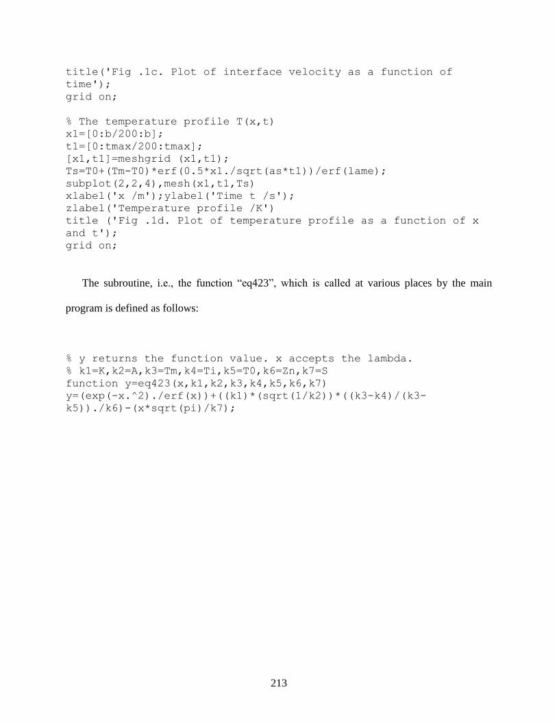
213
title('Fig .1c. Plot of interface velocity as a function of
time');
grid on;
% The temperature profile T(x,t)
x1=[0:b/200:b];
t1=[0:tmax/200:tmax];
[x1,t1]=meshgrid (x1,t1);
Ts=T0+(Tm-T0)*erf(0.5*x1./sqrt(as*t1))/erf(lame);
subplot(2,2,4),mesh(x1,t1,Ts)
xlabel('x /m');ylabel('Time t /s');
zlabel('Temperature profile /K')
title ('Fig .1d. Plot of temperature profile as a function of x
and t');
grid on;
The subroutine, i.e., the function ―eq423‖, which is called at various places by the main
program is defined as follows:
% y returns the function value. x accepts the lambda.
% k1=K,k2=A,k3=Tm,k4=Ti,k5=T0,k6=Zn,k7=S
function y=eq423(x,k1,k2,k3,k4,k5,k6,k7)
y=(exp(-x.^2)./erf(x))+((k1)*(sqrt(1/k2))*((k3-k4)/(k3-
k5))./k6)-(x*sqrt(pi)/k7);

214
Appendix B MATLAB Code for Implementing the LBM Solution
The extended LBGK equation based on a D1Q2 model to solve the unidirectional freezing of
water in a finite slab was coded up in MATLAB. In the code presented below, the subroutine
that was used for the analytic solution (Appendix A) is also included. During execution of the
code, a window will pop up to present the dynamic comparison between both solutions. The
details of the problem statement are available in Section 4.3.4.
clear all;close all;
% Define parameters
r_l=997;cp_l=4180;k_l=0.61;L=334000;
%Thermophysical properties of water
r_s=919;cp_s=2000;k_s=2.3;
%Thermophysical properties of ice
al_s=k_s/r_s/cp_s;al_l=k_l/r_l/cp_l;
Tm=273;T0=263;Ti=278;
%Freezing, boundary, and initial temps
tol=1e-8;dl=1e-8; %Tolerance, a small number
Hm_s=cp_s*Tm;
Hm_l=cp_l*Tm; %Enthalpy at melting temp.
Ste=cp_s*(Tm-T0)/L; %Stefan number
%Root-finding for the analytic solution
nn=4;lam=0.2; %Initial guess (important)
for j=1:100
lam(j+1)=lam(j)-
2*dl*tran(lam(j),k_l,k_s,al_l,al_s,Tm,T0,Ti,Ste,nn)/(tran(lam(j)
+dl,k_l,k_s,al_l,al_s,Tm,T0,Ti,Ste,nn)-tran(lam(j)-
dl,k_l,k_s,al_l,al_s,Tm,T0,Ti,Ste,nn));
if abs (lam(j+1)-lam(j))<tol;break;end
end
lam_exc=lam(j+1); %Exact value of lambda

215
beta=lam_exc+0.5*(nn+1)*(-
lam_exc+sqrt(lam_exc^2+2*nn*(al_l/al_s)/(nn+1)));
% Time and space meshing sizes
dx=1e-5; %Lattice interval
dt=1e-4; %Time step size
tau_l=0.5+al_l*dt/dx^2; %Thermal relaxation times
tau_s=0.5+al_s*dt/dx^2;
A1=0.5*r_l*cp_l*dx/dt;
A2=k_l/dx;
n=201; %Number of lattice points
i=10000; %Number of time steps
ul=zeros(i,n);ur=ul;T=ul; %Initiations for data storage
Texa=ul;Theta=T;
fl=ones(20,1);Ht=fl;Tt=fl;
%Liquid fraction and local enthalpy (liquid: 1, solid: 0)
f=ones(i,n);M=zeros(i,1);fexa=f;D=M; %Initial conditions
for a=1:n
ul(1,a)=0.5*Ti;
ur(1,a)=0.5*Ti;
end
% Time loops
for j=1:i
% Boundary conditions
ur(j,1)=T0-ul(j,1); %Left wall
ul(j+1,n)=0.5*((A1-A2)*(ul(j,n)+ur(j,n))+A2*(ul(j,n-
1)+ur(j,n-1)))/A1;
ur(j+1,n)=0.5*((A1-A2)*(ul(j,n)+ur(j,n))+A2*(ul(j,n-
1)+ur(j,n-1)))/A1;
ul(j,n)=ul(j+1,n);
ur(j,n)=ur(j+1,n); %Right wall (heat flux)
% Iteration for the solid-liquid interface, fl
for a=1:n
for ite=1:100 %Iteration for liquid fraction and temp
% Collison step
if f(j,a)>0.99
ul(j+1,a)=ul(j,a)+((0.5*(ul(j,a)+ur(j,a))-
ul(j,a))/tau_l)-0.5*(L/cp_l)*(fl(ite,1)-f(j,a));
ur(j+1,a)=ur(j,a)+((0.5*(ul(j,a)+ur(j,a))-
ur(j,a))/tau_l)-0.5*(L/cp_l)*(fl(ite,1)-f(j,a));
Tt(ite+1,1)=ul(j+1,a)+ur(j+1,a);
Ht(ite+1,1)=cp_l*Tt(ite+1,1)+L*fl(ite,1);
if Ht(ite+1,1)<Hm_l
fl(ite+1,1)=0;
elseif (Hm_l<=Ht(ite+1,1))&&(Ht(ite+1,1)<=Hm_l+L)

216
fl(ite+1,1)=(Ht(ite+1,1)-Hm_l)/L;
elseif Ht(ite+1,1)>Hm_l+L
fl(ite+1,1)=1;
end
f(j+1,a)=fl(ite+1,1);
Te=(Tt(ite+1,1)-Tt(ite,1))/Tt(ite,1);
fe=(fl(ite+1,1)-
fl(ite,1))/(fl(ite,1)+tol); %Relative error.
if (fe<=tol)&&(Te<=tol), break, end
elseif f(j,a)<=0.99
ul(j+1,a)=ul(j,a)+((0.5*(ul(j,a)+ur(j,a))-
ul(j,a))/tau_s)-0.5*(L/cp_s)*(fl(ite,1)-f(j,a));
ur(j+1,a)=ur(j,a)+((0.5*(ul(j,a)+ur(j,a))-
ur(j,a))/tau_s)-0.5*(L/cp_s)*(fl(ite,1)-f(j,a));
Tt(ite+1,1)=ul(j+1,a)+ur(j+1,a);
Ht(ite+1,1)=cp_s*Tt(ite+1,1)+L*fl(ite,1);
if Ht(ite+1,1)<Hm_s
fl(ite+1,1)=0;
elseif (Hm_s<=Ht(ite+1,1))&&(Ht(ite+1,1)<=Hm_s+L)
fl(ite+1,1)=(Ht(ite+1,1)-Hm_s)/L;
elseif Ht(ite+1,1)>Hm_s+L
fl(ite+1,1)=1;
end
f(j+1,a)=fl(ite+1,1);
Te=(Tt(ite+1,1)-Tt(ite,1))/Tt(ite,1);
fe=(fl(ite+1,1)-
fl(ite,1))/(fl(ite,1)+tol); %Relative errors.
if (fe<=tol)&&(Te<=tol), break, end
end
end
end
% Local temperature
T(j+1,:)=ul(j+1,:)+ur(j+1,:);
Theta(j+1,:)=(T(j+1,:)-T0)/(Ti-T0); %Non-dimensional
temperature
% Streaming step
ul(j+1,:)=circshift(ul(j+1,:),[0 -1]);
ur(j+1,:)=circshift(ur(j+1,:),[0 1]);
ul(j+1,n)=ul(j+1,n-1); %block the
communication from 1 to n;
% Exact solution
M(j+1)=2*lam_exc*sqrt(al_s*(j)*dt); %Melting front location
D(j+1)=2*beta*sqrt(al_s*(j)*dt); %Thermal penetration
front location

217
num_1=round(M(j+1)/dx);
num_2=round(D(j+1)/dx);
for a=1:num_1
Texa(j+1,a)=((Tm-T0)/(Ti-T0))*erf(0.5*(a-
1)*dx/sqrt(al_s*(j)*dt))/erf(lam_exc);
fexa(j+1,a)=0;
end
for a=num_1+1:num_2
Texa(j+1,a)=1-((Ti-Tm)/(Ti-T0))*((D(j+1)-(a-
1)*dx)/(D(j+1)-M(j+1)))^nn;
fexa(j+1,a)=1;
end
for a=num_2+1:n
Texa(j+1,a)=1;
fexa(j+1,a)=1;
end
% Illustration of temperature profiles
x=1e3*dx*[0:1:n-1];
subplot(2,1,1);plot(x,[Theta(j+1,:);Texa(j+1,:)],'LineWidth',1.5
);
xlabel('x(mm)','FontSize',18);ylabel('\theta','FontSize',18);
title(['After ' num2str(j) ' time steps'],'FontSize',18);
legend('LBM solution','Analytic solution');drawnow;
subplot(2,1,2);plot(x,[f(j+1,:);fexa(j+1,:)],'LineWidth',1.5);
xlabel('x (mm)','FontSize',18);ylabel('Liquid
fraction','FontSize',18);drawnow;
end
The function ―tran‖ is defined as:
function lam=tran(x,k_l,k_s,al_l,al_s,Tm,T0,Ti,Ste,nn)
Zn=(nn+1)*(-
x*sqrt(al_s/al_l)+sqrt(x^2*(al_s/al_l)+2*nn/(nn+1)))/nn/sqrt(pi);
lam=exp(-x^2)/erf(x)+(k_l/k_s)*sqrt(al_s/al_l)*((Tm-Ti)/(Tm-
T0))/Zn-x*sqrt(pi)/Ste;

218
Appendix C Predicted Thermophysical Properties of NePCM Samples
In this appendix, the predicted effective thermophysical properties of two representative
water- and cyclohexane-based NePCM samples considered in Chapter 4 are presented. The
thermophysical properties of base PCM (water and cyclohexane), in both liquid and solid phases,
are gathered in Table C.1. Due to the lack of actual thermophysical property data for nano-sized
materials, the thermophysical properties for the corresponding bulk materials were used in the
calculations for the nanoparticles. The thermophysical properties for the four materials (Al2O3,
Cu, CuO and TiO2) of nanoparticles considered in Chapter 4 are given in Table C.2.
For the given volume fractions (vol = 0, 1, 2, 5 and 10 vol%) of the nanoparticles, the
effective thermophysical properties of the NePCM samples were readily predicted using Eqs.
(4.63) to (4.67), which are listed in the following tables (Table C.3, Table C.4, Table C.5 and
Table C.6).

219
Table C.1 Thermophysical properties of water (ice) and cyclohexane
Properties
Water
(http://www.engineeringtoolbox.com/
water-thermal-properties-d_162.html, and
http://www.engineeringtoolbox.com/ ice-
thermal-properties-d_576.html)
Cyclohexane (C6H12)
(http://msds.chem.ox.ac.uk/
CY/cyclohexane.html, and
Sulfredge et al., 1993)
Liquid Solid (ice) Liquid Solid
(kg/m3) 997 919 779 856
Cp (J/kgK) 4,180 2,000 1,762.8 1,800
k (W/mK) 0.61 2.3 0.127 0.1359
L (J/kg) 334,000 32,557

220
Table C.2 Thermophysical properties of bulk materials for the nanoparticles considered
(Jang and Choi, 2007)
Properties Al2O3 Cu CuO TiO2
(kg/m3) 3,880 8,933 6,310 4,175
Cp (J/kgK) 792 385 540 692
k (W/mK) 42.34 401 18 8.4
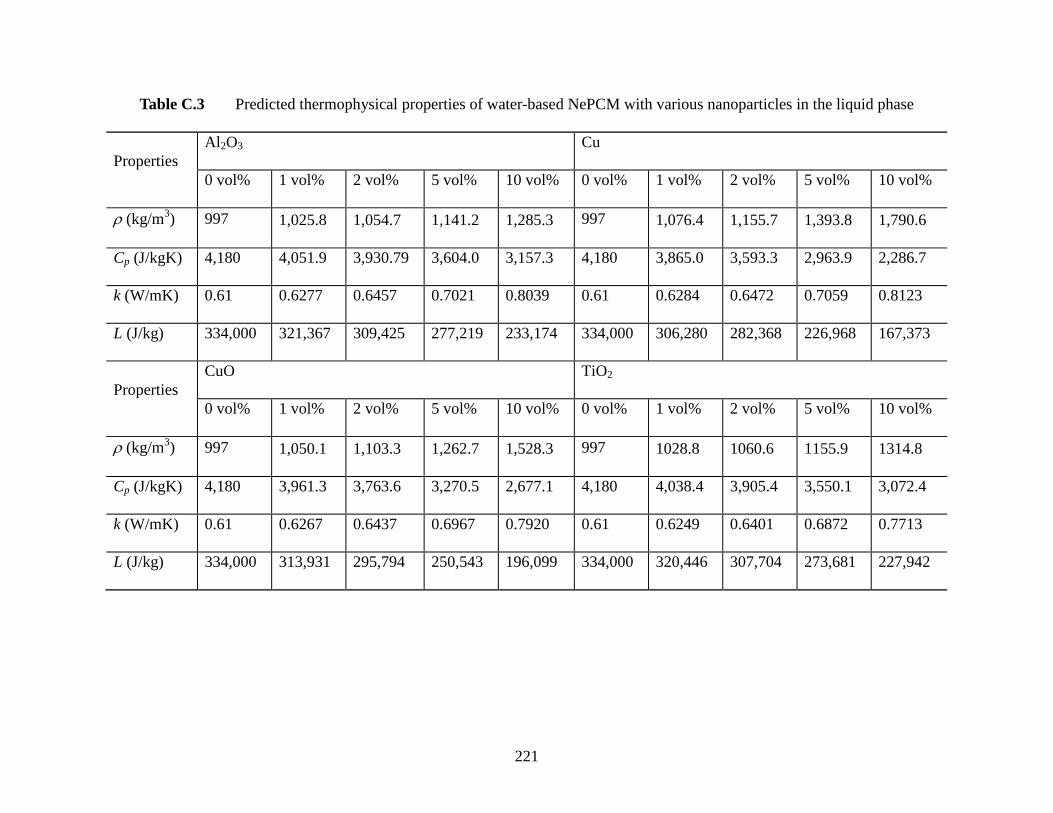
221
Table C.3 Predicted thermophysical properties of water-based NePCM with various nanoparticles in the liquid phase
Properties
Al2O3 Cu
0 vol% 1 vol% 2 vol% 5 vol% 10 vol% 0 vol% 1 vol% 2 vol% 5 vol% 10 vol%
(kg/m3) 997 1,025.8 1,054.7 1,141.2 1,285.3 997 1,076.4 1,155.7 1,393.8 1,790.6
Cp (J/kgK) 4,180 4,051.9 3,930.79 3,604.0 3,157.3 4,180 3,865.0 3,593.3 2,963.9 2,286.7
k (W/mK) 0.61 0.6277 0.6457 0.7021 0.8039 0.61 0.6284 0.6472 0.7059 0.8123
L (J/kg) 334,000 321,367 309,425 277,219 233,174 334,000 306,280 282,368 226,968 167,373
Properties
CuO TiO2
0 vol% 1 vol% 2 vol% 5 vol% 10 vol% 0 vol% 1 vol% 2 vol% 5 vol% 10 vol%
(kg/m3) 997 1,050.1 1,103.3 1,262.7 1,528.3 997 1028.8 1060.6 1155.9 1314.8
Cp (J/kgK) 4,180 3,961.3 3,763.6 3,270.5 2,677.1 4,180 4,038.4 3,905.4 3,550.1 3,072.4
k (W/mK) 0.61 0.6267 0.6437 0.6967 0.7920 0.61 0.6249 0.6401 0.6872 0.7713
L (J/kg) 334,000 313,931 295,794 250,543 196,099 334,000 320,446 307,704 273,681 227,942

222
Table C.4 Predicted thermophysical properties of water-based NePCM with various nanoparticles in the solid phase
Properties
Al2O3 Cu
0 vol% 1 vol% 2 vol% 5 vol% 10 vol% 0 vol% 1 vol% 2 vol% 5 vol% 10 vol%
(kg/m3) 919 948.6 978.2 1,067.1 1,215.1 919 999.1 1,079.3 1,319.7 1,720.4
Cp (J/kgK) 2,000 1,950.6 1,904.2 1,780.4 1,614.3 2,000 1,855.6 1,732.7 1,453.4 1,161.4
k (W/mK) 2.3 2.3594 2.4198 2.6074 2.9435 2.3 2.3685 2.4384 2.6567 3.0522
Properties
CuO TiO2
0 vol% 1 vol% 2 vol% 5 vol% 10 vol% 0 vol% 1 vol% 2 vol% 5 vol% 10 vol%
(kg/m3) 919 972.9 1,026.8 1,188.6 1,458.1 919 951.6 984.1 1,081.8 1,244.6
Cp (J/kgK) 2,000 1,905.3 1,820.6 1,612.4 1,368.2 2,000 1,942.6 1,889.0 1,747.6 1,561.2
k (W/mK) 2.3 2.3483 2.3972 2.5483 2.8151 2.3 2.3325 2.3654 2.4658 2.6397

223
Table C.5 Predicted thermophysical properties of cyclohexane-based NePCM with various nanoparticles in the liquid phase
Properties
Al2O3 Cu
0 vol% 1 vol% 2 vol% 5 vol% 10 vol% 0 vol% 1 vol% 2 vol% 5 vol% 10 vol%
(kg/m3) 779 810.0 841.0 934.1 1,089.1 779 860.5 942.1 1,186.7 1,594.4
Cp (J/kgK) 1,762.8 1,716.3 1,673.2 1,561.2 1,417.0 1,762.8 1,619.8 1,501.5 1,244.2 990.9
k (W/mK) 0.127 0.1308 0.1347 0.1469 0.1689 0.127 0.1308 0.1348 0.1470 0.1693
L (J/kg) 32,557 30,997 29,553 25,795 20,958 32,557 29,177 26,383 20,303 14,316
Properties
CuO TiO2
0 vol% 1 vol% 2 vol% 5 vol% 10 vol% 0 vol% 1 vol% 2 vol% 5 vol% 10 vol%
(kg/m3) 779 834.3 889.6 1,055.6 1,332.1 779 813.0 846.9 948.8 1,118.6
Cp (J/kgK) 1,762.8 1,670.3 1,589.3 1,397.3 1,183.6 1,762.8 1,707.8 1,657.2 1,527.2 1,363.1
k (W/mK) 0.127 0.1308 0.1346 0.1466 0.1684 0.127 0.1307 0.1344 0.1461 0.1673
L (J/kg) 32,557 30,095 27,939 22,826 17,135 32,557 30,885 29,347 25,394 20,406

224
Table C.6 Predicted thermophysical properties of cyclohexane-based NePCM with various nanoparticles in the solid phase
Properties
Al2O3 Cu
0 vol% 1 vol% 2 vol% 5 vol% 10 vol% 0 vol% 1 vol% 2 vol% 5 vol% 10 vol%
(kg/m3) 856 886.2 916.5 1,007.2 1,158.4 856 936.8 1,017.5 1,259.9 1,663.7
Cp (J/kgK) 1,800 1,716.3 1,673.2 1,561.2 1,417.0 1,800 1,619.8 1,501.5 1,244.2 990.9
k (W/mK) 0.1359 0.1401 0.1442 0.1573 0.1809 0.1359 0.1401 0.1443 0.1575 0.1813
Properties
CuO TiO2
0 vol% 1 vol% 2 vol% 5 vol% 10 vol% 0 vol% 1 vol% 2 vol% 5 vol% 10 vol%
(kg/m3) 856 910.5 965.1 1,128.7 1,401.4 856 889.2 922.4 1,022.0 1,187.9
Cp (J/kgK) 1,800 1,670.3 1,589.3 1,397.3 1,183.6 1,800 1,707.8 1,657.2 1,527.2 1,363.1
k (W/mK) 0.1359 0.1400 0.1441 0.1570 0.1802 0.1359 0.1399 0.1439 0.1564 0.1790

225
Appendix D Calibration of Thermocouples
Eight (8) K-type chromel-alumel thermocouples (TC) (PN: TT-K-30, Omega, Stamford, CT),
numbered from #0 to #7, were fabricated for use as the temperature sensors in the unidirectional
freezing experiment (Chapter 5). Prior to being mounted on the test cell, the TCs were calibrated
carefully against a high-accuracy ice point calibration cell (TRCIII, Omega, Stamford, CT).
The ice point afforded by the calibration cell was assured by a 2-wire thermistor (A733F-
CSP60BT103M, GE Sensing, St. Marys, PA) that has been calibrated to an accuracy of 0.01 °C.
The TCs were connected to a 16-channel data acquisition (DAQ) unit (NI 9213, National
Instruments, Austin, TX) that has a built-in cold junction compensation circuit.
The readings of the TCs in the calibration cell were recorded over 20 minutes (at an interval
of 5 s), which are presented in Figure D.1. It is shown that each TC had an individual
temperature shift from the ice point (0 °C). The shifts were calculated by comparing the time-
averaged readings over the 20 minutes against 0 °C, which are listed in Table D.1.
These shifts were used as compensation for correcting the raw TC data. For example, the
temperature readings of TC#5 must be corrected by adding 0.37717 °C. It is interesting that the
temperature shift grows monotonically grown with increasing TC number. This is because the
TCs were mounted in such an order that their terminals were located farther away from the built-
in cold junction, which in turn leads to the growing shift. As observed in Figure D.1, the
uncertainty of the readings of all the TCs was within 0.02 °C.

226
Table D.1 The measured temperature shifts of the eight (8) TCs against 0 °C
TC number Temperature shift (°C)
0 0.17129
1 0.25601
2 0.32445
3 0.34270
4 0.36660
5 0.37717
6 0.41650
7 0.43000

227
Figure D.1 Temperature histories of the eight (8) TCs recorded over 20 minutes while being calibrated using an ice point
calibration cell

228
Appendix E LabVIEW Virtual Instrument for Data Acquisition of Thermocouples
A 16-channel data acquisition (DAQ) unit (NI 9213, National Instruments, Austin, TX) was
used to log the TC readings. The DAQ unit was connected to a personal computer through a real-
time controller (NI cRIO-9014, National Instruments, Austin, TX) and was operated by a
LabVIEW-based virtual instrument (VI), as shown in Figure E.1.

229
Figure E.1 Block diagram of the LabVIEW VI for implementing real-time data acquisition of the TCs

230
Appendix F Uncertainty Analysis of the Experimental Results
In this appendix, an uncertainty analysis of the experimental results is presented following
the theory described by Coleman and Steele (1989).
In Chapter 3, the uncertainty of the thermal conductivity measurement for a sample was
represented by the standard deviation over the individual runs. The use of the standard deviation
absorbs all the possible systematic errors, such as data reduction from the TPS theory,
temperature control of the bath and accuracy of the instrument (2% as specified by the
manufacturer), etc.
In Chapter 5, however, the errors of the temperature recordings along the freezing direction
were attributed to two major factors: the accuracy of the TC readings and the location of the TC
junctions. As mentioned before, the uncertainty of the TC readings was ± 0.02 °C, whereas the
uncertainty of the location of TC junctions was ± 0.3 mm. Also note that these two factors were
independent with each other.

231
Appendix G Estimation of Time Response of Thermocouples
In this appendix, an analysis is performed to estimate the time response of the TCs that is
important for temperature measurements under transient conditions.
As described by Holman (1994), a lumped model analysis, as shown in Figure G.1, is
adopted to estimate the response time of a TC bead to the transient variation of ambient
temperature. The TC bead that is assumed to be always uniform in temperature (T) is exposed to
a sudden change in ambient temperature (T∞) for t > 0. As radiation heat transfer is ignored, the
bead is assumed to exchange heat with the ambient only through convection with a heat transfer
coefficient of h. The energy balance equation for the transient heat exchange process can be
written as
)( TThAtd
dTVC
p
, (G.1)
where ρ, V, Cp and A stand for the nominal density, volume, specific heat capacity and surface
area of the TC bead. The bead is subject to initial condition T(t = 0) = T0.
By solving Eq. (G.1), the transient temperature of the TC bead is obtained as:
)exp(0
tTT
TT
, (G.2)
where τ is time constant of the system (TC bead in this case), which is defined by
hA
VCp
, (G.3)
If a spherical bead of a radius R is considered, Eq. (G.3) is reduced to

232
h
RCp
3
, (G.4)
When t = 4.6τ, the bead temperature has reached approximately 99% of its final value (i.e.,
an error of 1%). At this instant, the bead temperature (i.e., the temperature reading of the TC) can
be considered as identical to the actual ambient temperature being measured.
For K-type TCs, the density and specific heat capacity of the bead are assumed to be 8,908
kg/m3 and 423 J/kgK, respectively. Here the properties of nickel (the dominant constituent of
both chromel and alumel, that are alloys made of about 90% and 95% nickel, respectively) at
room temperature are used (http://en.wikipedia.org/wiki/Nickel, and
http://www.kayelaby.npl.co.uk/general_physics/2_3/2_3_6.html). Also assuming that the
spherical bead has a radius of 0.3 mm and the heat transfer coefficient is 500 W/m2K and
substituting all the above parameters, the time constant is found to be approximately 0.754
second. Therefore, it takes about 3.5 second for the TC bead to be consistent with the actual
ambient temperature being measured. The validity of the lumped analysis can be checked by
calculating the Biot number (Bi) of the system, given by
k
hRBi , (G.5)
where the radius R of the bead is chosen as the characteristic length and k is the thermal
conductivity of the bead.
By adopting the thermal conductivity of chromel (19 W/mK, available at
http://en.wikipedia.org/wiki/Chromel), the Bi number is determined to be approximately 0.0079,
which is much less than 0.1 (Incropera et al., 2007). The applicability of the lumped analysis is
thus validated.
233
The analysis above gives a simple estimation of the temporal uncertainty of the TC readings.
The response time of the TCs being used is found to be of the same order of the temporal
resolution (5 second) of the logged data in the freezing experiments.
Also note that, as shown in Figure 5.1b, the TC beads were coated with a layer of epoxy of a
nominal thickness of 0.3 mm and were not directly exposed to the sample in the test cell. This
was done in order to avoid possible interactions of the TC beads with the hydrocarbon-based
colloids. Even though the epoxy is not very conductive (thermal conductivity of ~0.2 W/mK,
available at http://www.efunda.com/materials/polymers/properties/polymer_datasheet.cfm?
MajorID=epoxy&MinorID=8), the time lag of the temperature disturbance diffusing through the
epoxy layer is expected to be very short and would be absorbed into the time response of the
TCs. It is suggested that in order to avoid this issue and also possible formation of air pockets
within the epoxy, a new configuration of mounting the TCs on the unidirectional freezing test
cell, as shown in Figure G.2, might be explored.

234
Figure G.1 Schematic diagram of a lumped model for thermal response of a TC bead exposed
to a sudden change in ambient temperature

235
Figure G.2 Schematic diagram of a new configuration of mounting the TCs on the
unidirectional freezing test cell