Enhanced Reduction/Coagulation/ Filtration …mwdh2o.com/FAF PDFs/1a_GW_Glendale MWD Final Report.pdfEnhanced Reduction/Coagulation/ Filtration Testing for Removing Hexavalent Chromium

Enhanced Reduction/Coagulation/ Filtration Testing for Removing Hexavalent Chromium

Prepared by: Xueying (Ying) Wu, DEnv, PE Nicole Blute, PhD, PE Maggie Pierce, PE Marc Santos, PE Kenny Chau, PE David Rodriguez Hazen and Sawyer 1149 South Hill Street, Suite 450 Los Angeles, CA 90015 Charles Cron Dan Hutton, PE CDM Smith 800 Flower Street Glendale, California 91201 Leighton Fong, PE Donald Froelich, PE Leo Chan, PE Michael De Ghetto, PE City of Glendale 141 N. Glendale Avenue, 4th Level Glendale, California 91206 December 31, 2015

Sponsored by: Metropolitan Water District of Southern California California Department of Water Resources, Proposition 50

I

CONTENTS

TABLES ....................................................................................................................................... III

FIGURES ....................................................................................................................................... V

EXECUTIVE SUMMARY ............................................................................................................ 1

Objectives ........................................................................................................................... 1 Background ......................................................................................................................... 1 Approach ............................................................................................................................. 2 Results/Conclusions ............................................................................................................ 2

CHAPTER 1. INTRODUCTION ................................................................................................... 3

CHAPTER 2. COST SUMMARY ................................................................................................. 5

CHAPTER 3. SCHEDULE SUMMARY ....................................................................................... 6

CHAPTER 4. JAR TESTING OF RCF REDUCTION TIME AND IRON DOSE ...................... 7

Objectives ........................................................................................................................... 7 Materials and Methods ........................................................................................................ 7

Raw Water Quality ....................................................................................................... 7

Evaluation of Ferrous Iron Dose and Reduction Time ................................................. 8 Evaluation of Cr(III) Reoxidation by Chlorine in the RCF Process ............................. 8

Evaluation of Polymer Mixing Time ............................................................................ 9 Analytical Methods ..................................................................................................... 10

Results ............................................................................................................................... 11 Evaluation of Ferrous Iron Dose and Reduction Time ............................................... 11

Evaluation of Cr(III) Reoxidation by Chlorine in the RCF Process ........................... 14 Evaluation of Polymer Mixing Time .......................................................................... 16

Summary and Conclusions ............................................................................................... 19

CHAPTER 5. DEMONSTRATION TESTING OF RCF REDUCTION TIME AND IRON DOSE ............................................................................................................................................ 20

Objectives ......................................................................................................................... 20 Materials and Methods ...................................................................................................... 20

Raw Water Quality ..................................................................................................... 20 RCF Process ................................................................................................................ 21

Operational Conditions ............................................................................................... 21 Sampling and Monitoring ........................................................................................... 22 Analytical Methods ..................................................................................................... 23

Results ............................................................................................................................... 24 Cr(VI) Reduction by Ferrous Iron .............................................................................. 24

Ferrous Iron Oxidation by Chlorine ............................................................................ 25 Cr(III) Re-oxidation .................................................................................................... 27 Cr(VI) and Total Cr Removal ..................................................................................... 28


II

CHAPTER 6. DEMONSTRATION-SCALE TESTING OF RCF ALTERNATIVE PUMPING 31

Objectives ......................................................................................................................... 31 Materials and Methods ...................................................................................................... 31

Raw Water Quality ..................................................................................................... 31

RCF Process ................................................................................................................ 32 Operational Conditions ............................................................................................... 32 Sampling and Monitoring ........................................................................................... 33 Analytical Methods ..................................................................................................... 33

Results ............................................................................................................................... 33

Cr(VI) Reduction by Ferrous Iron .............................................................................. 33 Ferrous Iron Oxidation by Chlorine ............................................................................ 34 Cr(III) Re-oxidation .................................................................................................... 35 Cr(VI) and Total Cr Removal ..................................................................................... 36


CHAPTER 7. COST ANALYSIS ................................................................................................ 38

Methodology ..................................................................................................................... 38 Design Water Quality ....................................................................................................... 40

RCF ................................................................................................................................... 41 Capital Cost ................................................................................................................. 43 O&M Cost ................................................................................................................... 45

Unit Treatment Cost .................................................................................................... 46 SBA ................................................................................................................................... 47

Capital Cost ................................................................................................................. 50 O&M Cost ................................................................................................................... 52

Unit Treatment Cost .................................................................................................... 54 WBA ................................................................................................................................. 54

Capital Cost ................................................................................................................. 56 O&M Cost ................................................................................................................... 57 Unit Treatment Cost .................................................................................................... 59

UNIT COST COMPARISON FOR RCF, SBA AND WBA ........................................... 59

CHAPTER 8. LAYOUTS AND DRAWINGS ............................................................................ 61

RCF ............................................................................................................................. 61 SBA ............................................................................................................................. 61

WBA ........................................................................................................................... 61

CHAPTER 9. BLENDING ANALYSIS ...................................................................................... 74

Methodology ..................................................................................................................... 74 Scenario 1. Baseline .......................................................................................................... 76 Scenario 2. Effects of Water Quality ................................................................................ 78 Scenario 3. Effects of Treatment Goal .............................................................................. 80 Summary and Conclusions ............................................................................................... 86

CHAPTER 10. SUMMARY AND CONCLUSIONS .................................................................. 87

CHAPTER 11. REFERENCES .................................................................................................... 89

III

TABLES

Table 1. Summary of Costs and Funds as of September 30, 2015 ................................................. 5 Table 2. Raw Water Quality ........................................................................................................... 7 Table 3. Test Matrix for Ferrous Iron Doses and Reduction Times ............................................... 8 Table 4. Test Matrix for Evaluating Cr(III) Re-oxidation to Cr(VI) by Chlorine .......................... 9 Table 5. Test Matrix for Evaluating Polymer Mixing Time ........................................................... 9

Table 6. Analytical Methods ......................................................................................................... 10 Table 7. Chlorine Residual for Chlorine Doses of 1.0 and 2.0 mg/L in Lower Cr(VI) Water ..... 14 Table 8. Raw Water Quality for Demonstration Testing with the Progressive Cavity Pump ...... 20 Table 9. Operational Conditions of Demonstration RCF with Progressive Cavity Pump ............ 22 Table 10. Sampling and Analysis for Demonstration RCF with a Progressive Cavity Pump ...... 23

Table 11. Analytical Methods ....................................................................................................... 23 Table 12. Cr(VI) at Post Reduction for Demonstration RCF with Progressive Cavity Pump ...... 24

Table 13. Chlorine Dose and Residuals for Demonstration RCF with a Progressive Cavity Pump....................................................................................................................................................... 25

Table 14. Average Cr(VI) Concentrations of Individual Monitoring Locations of Each Run ..... 27 Table 15. Raw Water Quality for Demonstration Testing with Centrifugal Pumping ................. 31

Table 16. Operational Conditions of Demonstration RCF with Centrifugal Pumping ................. 32 Table 17. Cr(VI) at Post Reduction for Demonstration RCF with Centrifugal Pumping ............. 33 Table 18. Chlorine Dose and Residuals for Demonstration RCF with Centrifugal Pumping ...... 34

Table 19. Average Cr(VI) Concentrations of Individual Monitoring Locations of Each Run ..... 35 Table 20. Capital Cost Factors Assumptions ................................................................................ 39

Table 21. Engineering Factors Assumptions ................................................................................ 40

Table 22. Design Raw Water Quality for RCF, WBA and SBA .................................................. 41

Table 23. RCF Design Criteria ..................................................................................................... 43 Table 24. RCF Capital Costs ........................................................................................................ 44

Table 25. RCF Annual O&M Costs .............................................................................................. 46 Table 26. RCF 20-year NPV of O&M Costs ................................................................................ 46 Table 27. RCF Unit Treatment Costs ($/AF)................................................................................ 46

Table 28. SBA Regeneration Procedure Used for Cost Estimates ............................................... 49

Table 29. SBA Design Criteria ..................................................................................................... 50 Table 30. SBA Capital Costs ........................................................................................................ 51 Table 31. SBA Annual O&M Costs ............................................................................................. 53 Table 32. SBA 20-year NPV of O&M Costs ................................................................................ 53 Table 33. SBA Unit Treatment Costs ($/AF) ............................................................................... 54

Table 34. WBA Design Criteria .................................................................................................... 56 Table 35. WBA Capital Costs ....................................................................................................... 57

Table 36. WBA Annual O&M Costs ............................................................................................ 58 Table 37. WBA 20-year NPV of O&M Costs .............................................................................. 58 Table 38. WBA Unit Treatment Costs ($/AF) .............................................................................. 59 Table 39. Overview of Scenarios .................................................................................................. 74 Table 40. Design Water Quality for Scenario 1 Baseline ............................................................. 77

Table 41. Scenario 1 Results – Blending versus Non-Blending ................................................... 77 Table 42. Blending versus Non-Blending for WBA with Different Alkalinity Concentrations .. 79 Table 43. Blending versus Non-Blending for SBA with Different Sulfate Concentrations ......... 80

IV

Table 44. Assumed WBA Resin Bed Volumes for Different Cr(VI) Treatment Goals ............... 81

Table 45. Blending versus Non-Blending for WBA with Different Treatment Goals ................. 82 Table 46. Blending versus Non-Blending for SBA with Different Treatment Goals ................... 83 Table 47. Blending versus Non-Blending for RCF with Different Treatment Goals ................... 84

V

FIGURES

Figure 1. Project Schedule Summary.............................................................................................. 6 Figure 2. Cr(VI) Concentrations Post Reduction and before Chlorine Addition for Low Cr(VI) Water ............................................................................................................................................. 11 Figure 3. Cr(VI) Concentrations Post Reduction and before Chlorine Addition for High Cr(VI) Water ............................................................................................................................................. 12

Figure 4. Total Cr Concentrations in 1 µm Filtered Samples for Lower Cr(VI) Water ............... 12 Figure 5. Total Cr Concentrations in 0.1 µm Filtered Samples for Lower Cr(VI) Water ............ 13 Figure 6. Total Cr Concentrations in 1 µm Filtered Samples for Higher Cr(VI) Water .............. 13 Figure 7. Total Cr Concentrations in 0.1 µm Filtered Samples for Higher Cr(VI) Water ........... 14 Figure 8. Cr(VI) Concentrations with Various Chlorine Doses and Contact Times for Lower Cr(VI) Water ................................................................................................................................. 15 Figure 9. Cr(VI) Concentrations with Various Chlorine Doses and Contact Times for Higher Cr(VI) Water ................................................................................................................................. 16 Figure 10. Total Cr Concentrations in 1 µm Filtered Water for the Polymer Mixing Test for Lower Cr(VI) Water ..................................................................................................................... 17 Figure 11. Total Cr Concentrations in 0.1 µm Filtered Water for the Polymer Mixing Test for Lower Cr(VI) Water ..................................................................................................................... 17 Figure 12. Total Cr Concentrations in 1 µm Filtered Water for the Polymer Mixing Test for Higher Cr(VI) Water ..................................................................................................................... 18

Figure 13. Total Cr Concentrations in 0.1 µm Filtered Water for the Polymer Mixing Test for Higher Cr(VI) Water ..................................................................................................................... 18

Figure 14. Schematic of RCF Process Evaluated with a Progressive Cavity Pump ..................... 21

Figure 15. Cr(VI) Results at Post Reduction for Demonstration RCF with Progressive Cavity Pump ............................................................................................................................................. 25 Figure 16. Chlorine Residual at Post Chlorination for Demonstration RCF with Progressive Cavity Pump.................................................................................................................................. 26 Figure 17. Average Cr(VI) Concentrations of Individual Monitoring Locations of Each Run .... 28 Figure 18. Cr(VI) Concentrations in Filter Effluent ..................................................................... 29

Figure 19. Total Cr Concentrations in Filter Effluent................................................................... 29

Figure 20. RCF Process Schematic with a Centrifugal Pump ...................................................... 32 Figure 21. Cr(VI) Results at Post Reduction for Demonstration RCF with a Centrifugal Pump . 34 Figure 22. Chlorine Residual at Post Chlorination for Demonstration RCF with Centrifugal Pumping ........................................................................................................................................ 35 Figure 23. Average Cr(VI) Concentrations of Individual Monitoring Locations of Each Run .... 36

Figure 24. Cr(VI) Concentrations in Filter Effluent ..................................................................... 37 Figure 25. Total Cr Concentrations in Filter Effluent................................................................... 37

Figure 26. Approach for Developing RCF, WBA and SBA Estimates ........................................ 39 Figure 27. RCF Process Flow Diagram ........................................................................................ 42 Figure 28. RCF Unit Treatment Costs .......................................................................................... 47 Figure 29. SBA Process Flow Diagram ........................................................................................ 48 Figure 30. SBA Residual Treatment Process Flow Diagram ....................................................... 49

Figure 31. SBA Bed Volumes as a Function of Sulfate Concentration for Cr(VI) Breakthrough 53 Figure 32. SBA Unit Treatment Costs .......................................................................................... 54 Figure 33. WBA Process Flow Diagram ...................................................................................... 55

VI

Figure 34. WBA Unit Treatment Costs ........................................................................................ 59

Figure 35. RCF, SBA and WBA Unit Treatment Costs ............................................................... 60 Figure 36. RCF Without Recycle Site Plan .................................................................................. 62 Figure 37. RCF Without Recycle Equipment Layout ................................................................... 63

Figure 38. RCF Without Recycle PFD ......................................................................................... 64 Figure 39. RCF With Recycle Site Plan ....................................................................................... 65 Figure 40. RCF With Recycle Equipment Layout ........................................................................ 66 Figure 41. RCF With Recycle PFD .............................................................................................. 67 Figure 42. SBA Site Plan .............................................................................................................. 68

Figure 43. SBA Equipment Layout .............................................................................................. 69 Figure 44. SBA PFD ..................................................................................................................... 70 Figure 45. WBA Site Plan ............................................................................................................ 71 Figure 46. WBA Equipment Layout ............................................................................................. 72

Figure 47. WBA PFD ................................................................................................................... 73 Figure 48. Capital Cost Curves for RCF with and without Recycle ............................................. 75

Figure 49. Capital Cost Curves for WBA and SBA ..................................................................... 75 Figure 50. Approach Used to Estimate Treatment Flow Rate ...................................................... 76

Figure 51. Treatment Costs for Blending vs. Non-Blending in Scenario 1 .................................. 78 Figure 52. Effect of Alkalinity on WBA Treatment Costs for Blending vs. Non-Blending ........ 79 Figure 53. Effect of Sulfate on SBA Treatment Costs for Blending vs. Non-Blending ............... 80

Figure 54. SBA Bed Volumes as a Function of Sulfate Concentration for Cr(VI) Breakthrough Greater than 4, 6, and 8 µg/L ........................................................................................................ 81

Figure 55. Effect of Treatment Goal on WBA Treatment Costs for Blending vs. Non-Blending 82 Figure 56. Effect of Treatment Goal on SBA Treatment Costs for Blending vs. Non-Blending . 83 Figure 57. Effect of Treatment Goal on RCF Treatment Costs for Blending vs. Non-Blending . 84

1

EXECUTIVE SUMMARY

Hexavalent chromium, Cr(VI), is now regulated by the State of California as of July 1, 2014. Best Available Technologies identified by the State for Cr(VI) removal from drinking water include ion exchange (weak base anion, WBA, or strong base anion, SBA), coagulation and filtration with upstream reduction (RCF), and reverse osmosis (RO). Extensive research has been completed by the City of Glendale with other partners to determine the effectiveness of each treatment process with respect to water quality and treatment robustness. The RCF process was identified as offering potential opportunities for treatment optimization to decrease cost and footprint, but required additional testing.

OBJECTIVES

The objectives of this study were to test potential improvements in the RCF process for removing Cr(VI) from drinking water, and compare this approach with other leading technologies. Specific objectives completed included:

Systematic assessment of the impact of reduction time and iron dose on the RCF process, Evaluation of the cost competitiveness of enhanced RCF compared with WBA and SBA, Comparison of technology site layouts and preliminary design drawings of the enhanced

RCF process with the WBA and SBA processes, and Testing of an alternative RCF pumping approach for cost savings.

BACKGROUND

A new Cr(VI) maximum contaminant level (MCL) of 10 µg/L was released in California, affecting many drinking water utilities who rely on local groundwater as their source of supply. Improved treatment options were identified as a need to enhance feasibility of treatment implementation by water agencies.

Two types of anion exchange, WBA and SBA, have been proven to be effective for

Cr(VI) removal. WBA offers a relatively simple, once-through treatment approach. Limitations of WBA include pH adjustment requirements for sources that have high alkalinity. SBA can be operated in two different modes – as single-pass media or with periodic regeneration using salt brine solution. The single-pass operation is advantageous where space is a premium, but operations costs can be very high. Regenerable SBA generates hazardous waste brine that requires treatment and/or disposal of the brine offsite. Operating conditions and design parameters of both technologies have been well established as a viable option for effective Cr(VI) removal. RCF treatment has also been proven to be effective but requires a large footprint as a result of the multi-step unit processes, and as a result, this option may be difficult to implement at small well sites. The process requires ferrous iron to be dosed in the source water and react in a reduction tank, followed by oxidation of the excess ferrous with either oxygen or chlorine. Polymer is then added to coagulate the iron and Cr particles, which are removed by a filtration process. Previous demonstration-scale testing was carried out for the RCF process using a 45-

2

minute reduction time and was proven to be effective in Cr(VI) removal. The need to evaluate the process for potential improvements was identified to offer overall footprint reduction and cost savings.

APPROACH

The approach taken to evaluate the potential improvements on the RCF process in this study included the following tasks:

Task 1 – Systematically assess the impact of reduction time and iron dose on the RCF

process via bench-scale testing, followed by demonstration-scale testing Task 2 – Evaluate cost competitiveness of enhanced RCF compared with WBA and SBA Task 3 – Develop technology site layouts and preliminary design drawings for enhanced

RCF compared with WBA and SBA Task 4 – Test an alternative RCF pumping approach for potential cost savings Task 5 – Identify opportunities for water systems to use blending to achieve compliance

with the Cr(VI) MCL Task 6 – Project management (Glendale)

RESULTS/CONCLUSIONS

Bench-scale testing assessed the impact of lower reduction times (1, 5 and 15-minute) and ferrous iron dosing (1.5, 2.0 and 3.0 mg/L). The results showed that a ferrous dose of 2 mg/L or above was effective in Cr(VI) reduction down to less than 1 µg/L for low Cr(VI) impacted sources (15 µg/L). A higher dose of 3 mg/L of ferrous iron was required for higher concentrations (100 µg/L). A 1-minute reduction time was insufficient for Cr(VI) reduction to Cr(III), but 5 and 15 minutes were effective. Oxidation with chlorine did not result in significant re-oxidation of Cr(III) to Cr(VI) in the time scales tested at the bench scale.

At the demonstration scale (100 gpm), the effectiveness of the RCF process for 5 or 15

minutes of reduction time and an iron dose of 2 to 3 mg/L was confirmed. Effective ferrous iron oxidation was achieved in this study using inline chlorine addition, compared with prior testing using a chlorine contact tank. Cr(III) re-oxidation was consistent with the bench-scale results and was proven to be small (less than 1.5 µg/L) except for 1 minute reduction time.

A centrifugal pump was tested in place of the progressive cavity pump used in prior

demonstration-scale testing. Cr(III) particles were effectively removed by granular media filtration with centrifugal pumping and the filtered Cr(VI) and total Cr concentrations were below 3 µg/L. The results are similar to the results for the progressive cavity pumping tests, suggesting that centrifugal pumping could replace progressive cavity pumping for cost savings without significantly deteriorating Cr removal.

Using the results of this study and other recent work, Cr(VI) treatment costs were

updated and compared. A blending analysis was also completed to evaluate the potential for additional cost savings when comparing blending with a non-blending (full treatment) approach. Overall, the unit treatment cost of the blending approach was significantly lower for all three technologies regardless of water quality and extent of treatment.

3

CHAPTER 1. INTRODUCTION

Coagulation with filtration and upstream reduction (reduction/coagulation/filtration, or RCF) is a Best Available Technology (BAT) listed by the State of California for removal of hexavalent chromium, Cr(VI), from drinking water. The process consists of ferrous iron addition that reduces Cr(VI) to Cr(III), aeration or chlorination to oxidize remaining ferrous iron, polymer addition and mixing, and filtration. In previous demonstration-scale testing at the City of Glendale, the RCF process was proven to effectively remove Cr(VI) to below 1 µg/L and Total Cr to below 5 µg/L, with 30 and 45-minute reduction times and 5-minute aeration time. However, the process in that configuration requires a relatively large footprint, which limits its applicability for many groundwater systems.

In a demonstration-scale study completed in 2013, RCF was tested using a dose of 3

mg/L ferrous iron, lower reduction times (30, 15 and 5 minutes) and chlorination (in place of aeration for ferrous oxidation) for a water source containing approximately 100 µg/L of Cr(VI). The results were promising for RCF enhancement with a lower reduction time and chlorination, which would significantly reduce the process footprint, operation complexity, and capital expenditures. The results also indicated that Cr(III) re-oxidation by chlorine occurred at times. More extensive evaluation at the demonstration scale was identified as necessary to further evaluate reduction times and iron dose.

This study was designed with the following tasks to test an enhanced RCF process and compare technology costs.

Task 1 – Systematically assess the impact of reduction time and iron dose on the RCF

process via bench-scale testing, followed by demonstration-scale testing Task 2 – Evaluate cost competitiveness of enhanced RCF compared with WBA and SBA Task 3 – Develop technology site layouts and preliminary design drawings for enhanced

RCF compared with WBA and SBA Task 4 – Test an alternative RCF pumping approach for potential cost savings Task 5 – Identify opportunities for water system to use blending to achieve compliance

with the Cr(VI) MCL Task 6 – Project management (Glendale)

Task 1 of this study tested the interrelationship of ferrous iron dose and reduction time

coupled to Cr(VI) removal. This task consisted of bench-scale testing and demonstration-scale testing. Findings from the bench-scale testing provided the basis for selecting demonstration-scale test conditions. The testing approach and findings of the bench-scale study are discussed in Chapter 4 and the performance of the demonstration-scale study compared to the bench-scale test is discussed in Chapters 5 and 6. The outcome of this task was a better understanding of the tradeoffs in reduction time compared with iron dose, and the use of inline chlorination to oxidize excess ferrous without oxidizing Cr(III) to Cr(VI).

Task 2 of this study evaluated the cost competitiveness of enhanced RCF compared with

WBA and SBA based on the findings that from demonstration-scale tests. The primary focus of

4

this task was to refine the cost estimates for RCF based on findings in Task 1. SBA cost analyses were also prepared to provide an apples-to-apples comparison with RCF and WBA. Detailed cost analyses are provided in Chapter 7.

Task 3 involved the development of preliminary design drawings and site layouts for each process to provide a basis for comparing the space and ancillary requirements. The findings from Task 1 were used to develop facility site layouts and preliminary design drawings for a 1,000 gpm system for the enhanced RCF process. This process layout was compared with WBA and SBA site layouts based on a 1,000 gpm facility. The site layouts are provided in Chapter 8. Task 4 investigated an alternative pumping approach for the RCF process for potential cost savings. Initial cost estimates identified pumping as a major cost component that could be reduced if the alternative pump were to yield comparable performance by not breaking up flocculated particles too significantly for effective filtration of the coagulated total Cr and iron. Chapter 6 discusses the performance of the alternative pump compared to the findings from the demonstration-scale study described in Task 1 (Chapter 5).

Task 5 evaluated the opportunities for water systems to use blending to achieve the Cr(VI) MCL. Cost analysis was also completed in response to State’s interest in the cost implications of partial stream treatment (i.e., blending) to decrease costs and comply with the MCL, which is presented in Chapter 9.

Task 6 is a task performed by the City of Glendale (California) to manage the research

activities throughout the study period.

5

CHAPTER 2. COST SUMMARY

The overall budget for this research was $360,000 with $180,000 from California Proposition 50 administered by the California Department of Water Resources (DWR), and $180,000 by funding from Metropolitan Water District of Southern California (MWD). Table 1 summarizes the costs incurred and the funds disbursed throughout the project as of December 31, 2015, compared to the planned budget. The expenditures through December 31, 2015 amounted to $362,030.53 compared to an original budget of $360,000.

The costs for the individual tasks were different from the original task budgets as follows:

The CDM costs under Tasks 1 and 4 were greater than originally anticipated mainly due to the setup costs of the centrifugal pump were greater than expected and issues experienced with the system operation and control.

City of Glendale Water and Power (GWP) project management costs were lower than estimated because of the reduced need for GWP involvement in the effort.

Table 1. Summary of Costs and Funds as of December 31, 2015 Task No.

Proposed Budget Actual Costs Incurred

Funds Disbursed Total Project Funding from

MWD 1 $150,000 $75,000 $178,374,26 $178,374,26

2 $25,000 $12,500 $28,750.50 $28,750.50

3 $25,000 $12,500 $22,336.50 $22,336.50

4 $85,000 $42,500 $89,160.07 $89,160.07

5 $20,000 $10,000 $19,222.00 $19,222.00

6 $55,000 $27,500 $24,187.20 $24,187.20

Total $360,000 $180,000 $362,030.53 $362,030.53

6

CHAPTER 3. SCHEDULE SUMMARY

The project schedule is summarized in Figure 1. The overall project was completed as scheduled, although some tasks were delayed by well rehabilitation activities at the Glendale Operable Unit and operational challenges associated with aging equipment. Well rehabilitation activities impacted the test water availability thus demonstration testing until August 2014. In addition, two major challenges were experienced during demonstration testing, including chlorine feed pump and progressive cavity pump malfunction. These challenges were overcome by pump replacement and updating pump control programming. All tasks were affected by the delayed demonstration testing. Details are described in the third quarterly progress report of 2014. The project report was completed before the final deadline of February 1, 2016.

Figure 1. Project Schedule Summary

Task J F M A M J J A S O N D J F M A M J J A S O N D J F M

Task 1. RCF Process Enhancement

1.1. Bench Testing

1.2. Demonstration Testing - 6 Weeks

Task 2. Cost Competitiveness Analysis

2.1. RCF Cost Analysis

2.2. SBA Cost Analysis

Task 3. Site Layouts and Preliminary Design

Task 4. Alternative Pumping Approach

Task 5. Evaluate Blending Opportunities

Task 6. Glendale Project Management and Research

Reporting

Quarterly Report

Draft Report

Final Report

Original schedule from agreement

Actual schedule

Actual schedule

Q1

20162014

Q1 Q2 Q3 Q4 Q1 Q2 Q3

2015

Q4

7

CHAPTER 4. JAR TESTING OF RCF REDUCTION TIME AND IRON DOSE

This chapter summarizes the jar testing for evaluation of RCF reduction time and iron dose, which is a part of Task 1.

OBJECTIVES

The jar testing objectives included the following: Test multiple iron doses and reduction times to evaluate the interrelationship of

ferrous iron dose and reduction time, Evaluate if Cr(III) re-oxidation to Cr(VI) occurs by chlorine under conditions that

may be encountered in the RCF process, and Evaluate the effects of polymer mixing time on Cr(VI) removal to see if the five-

minute mixing time can be decreased.

MATERIALS AND METHODS

This section describes the raw water quality, jar testing procedures, and analytical methods. Three tests were conducted, including evaluation of ferrous iron dose and reduction times, Cr(III) re-oxidation, and polymer mixing time.

Raw Water Quality

Two raw waters with different Cr(VI) concentrations were tested as summarized in Table 2. The waters were obtained from different blends of the Glendale wells in the North Operable Unit, which had generally similar water quality but different Cr(VI) concentrations. The lower Cr(VI) water contained an average Cr(VI) of 16 µg/L. The higher Cr(VI) water averaged 100 µg/L. pH, temperature, turbidity and total iron were similar for the two waters.

Table 2. Raw Water Quality Parameter (units) Lower Cr(VI) Water Higher Cr(VI) Water

Average* Range* Average^ Range^

Cr(VI) (µg/L) 16 15 - 17 100 100 Cr, Total (µg/L) 16 15 - 18 110 110 pH 7.5 7.3 – 7.6 7.6 7.4 – 7.8 Temperature (⁰C) 20.3 19.6 – 20.4 22.1 21.7 – 22.4 Turbidity (NTU) 0.29 0.23 – 0.36 0.37 0.17 – 0.94 Iron, Total (mg/L) <0.02 <0.02 <0.02 <0.02

*Tested on the dates when jar testing was conducted, i.e. February 7th, 20th and 27th, 2014. ^Tested on the dates when jar testing was conducted, i.e. July 14th, 15th, 17th and 21st, 2014.

8

Evaluation of Ferrous Iron Dose and Reduction Time

Jar testing was performed using a Phipps & Bird jar tester to simulate demonstration-scale conditions. The ferrous doses and reduction times tested are summarized in Table 3, which were selected based on previous demonstration-scale results in which a higher influent Cr(VI) water source containing 100 µg/L was used. The previous results indicated that Cr(VI) could be reduced in 5 minutes by 3 mg/L ferrous iron.

Table 3. Test Matrix for Ferrous Iron Doses and Reduction Times

Ferrous Iron Dose

Target (mg/L)

Iron Dose Achieved for Lower

Cr(VI) Water

(mg/L)*

Iron Dose Achieved

for Higher Cr(VI) Water

(mg/L)*

Reduction Times

1 minute 5 minutes 10 minutes 15 minutes

1.5 1.4 1.5 X X X X 2.0 2.0 2.0 X X X X 3.0 2.7 2.8 X X X X

*Total iron concentration tested after 1 minute of fast mixing. The test procedure included the following steps:

1. The ferrous iron dose was added to a one-liter raw water sample, which was then rapidly mixed for one minute.

2. The sample was slowly mixed to simulate the coagulation process for the selected reduction time. Ferrous iron residual was tested at the end of the reduction time. Total iron was tested to confirm the iron dose. A Cr(VI) sample was collected for laboratory analysis to confirm that Cr(VI) was reduced to Cr(III).

3. A chlorine dose was added to achieve a free chlorine residual of 0.2 mg/L, followed by one minute of rapid mix. Ferrous iron was tested to confirm ferrous was all converted to ferric iron. A Cr(VI) sample was collected for laboratory analysis.

4. A polymer dose of 0.1 mg/L was added, followed by one minute of rapid mix and four minutes of slow mix (i.e., a total of five minutes to simulate the mixing time at the demonstration scale).

5. The sample was filtered through a 1 µm filter to represent granular media filtration and a 0.1 µm filter to represent microfiltration. Filtered water was tested for total iron, turbidity, chlorine, Cr(VI) and total Cr.

Evaluation of Cr(III) Reoxidation by Chlorine in the RCF Process

Table 4 summarizes the chlorine residual concentrations and reaction times tested to evaluate Cr(III) re-oxidation to Cr(VI) by chlorine. In prior testing, less than 0.5 mg/L chlorine residual was targeted to minimize Cr(III) re-oxidation, although no rigorous testing had shown what this maximum level could be without re-oxidation.

9

Table 4. Test Matrix for Evaluating Cr(III) Re-oxidation to Cr(VI) by Chlorine Chlorine Residual Target (mg/L)

Chlorine Dose

Added* (mg/L)

Chlorine Residual

Achieved^ (mg/L)

Reaction Times

5 minutes 10 minutes 15 minutes 30 minutes

0 (control) 0 <0.02 X X X X 0. 5 0. 5 0.46 X X X X 0.75 0.75 0.68 X X X X 1.0 1.0 0.87 X X X X 1.5 1.5 1.20 X X X X 2.0 2.0 1.60 X X X X

*The chlorine dose was equivalent to the chlorine residual target as ferrous iron was non-detect after reduction and the chlorine demand was negligible.

^Chlorine residual concentrations tested after 1 minute of fast mixing in the higher Cr(VI) water test, with the same chlorine doses applied in the column to the left.

The test procedure included the following steps:

1. A ferrous iron dose of 2.0 mg/L was added to a one-liter raw water sample, which was rapidly mixed for one minute.

2. The sample was slowly mixed for 15 minutes to simulate the coagulation process. Ferrous iron residual was tested at the end of the reduction time. Total iron was tested to confirm the iron dose. A Cr(VI) sample was collected for laboratory analysis to confirm Cr(VI) was reduced.

3. A chlorine dose was added to achieve the target chlorine residual, followed by one minute of rapid mix.

4. Cr(VI) samples were collected at 5, 10, 15 and 30 minutes for laboratory analysis. Total Cr was not analyzed as it was not expected to be removed without filtration.

Evaluation of Polymer Mixing Time

Table 5 summarizes the polymer mixing times tested to evaluate the effects of mixing time on Cr(VI) and total Cr removal. A polymer dose of 0.1 mg/L was tested, which is the dose applied at the Glendale demonstration scale. A set of samples without polymer was included as a control.

Table 5. Test Matrix for Evaluating Polymer Mixing Time

Polymer Dose (as active polymer)

Mixing Times*

1 minute 3 minutes 5 minutes 0 (control) X X X 0.1 mg/L X X X

*Including one-minute of rapid mix.

10

The test procedure included the following steps:

A ferrous iron dose of 2.0 mg/L was added to a one-liter raw water sample, which was rapidly mixed for one minute.

The sample was slowly mixed for 15 minutes to simulate the coagulation process. Ferrous iron residual was tested at the end of the reduction time. Total iron was tested to confirm the iron dose.

A chlorine dose was added to achieve a free chlorine residual of 0.2 mg/L, followed by a one minute rapid mix.

A polymer dose of 0.1 mg/L was added, followed by one minute rapid mix and then slow mixing to the time tested.

Samples were filtered through 1 µm and 0.1 µm filters. Filtered waters were tested for total iron, turbidity, chlorine, Cr(VI) and total Cr.

Analytical Methods

Table 6 summarizes the analytical methods for field and laboratory analysis.

Table 6. Analytical Methods Analyte Analysis

Location Analytical Method Method

Reporting Limit Cr(VI) Field Hach Method 8023 10 µg/L Cr(VI) Lab EPA 218.6 0.02 µg/L Total Cr Lab EPA 200.8 with acid

digestion 0.2 µg/L

Free Chlorine Field Hach Method 8021 0.02 mg/L Iron, Ferrous Field Hach Method 8146 0.02 mg/L Iron, Total Field Hach Method 8008 0.02 mg/L Iron, Total Lab EPA 200.7 0.05 mg/L pH Field SM 4500H+ B N/A Temperature Field SM 2550 N/A Turbidity Field SM 2130B / Hach 2100Q 0.02 NTU

EPA - United States Environmental Protection Agency SM - Standard Methods N/A - Not applicable

11

RESULTS

The jar testing results are summarized and discussed in this section.

Evaluation of Ferrous Iron Dose and Reduction Time

Figure 2 shows Cr(VI) concentrations after the reduction time with ferrous iron (1, 5, 10 and 15 minutes) and before chlorine addition, for the lower Cr(VI) water. With a ferrous dose of 1.5 mg/L, Cr(VI) in the range of 0.8 – 2.3 µg/L was still present, suggesting incomplete Cr(VI) reduction of the 15 – 17 µg/L initially present. With a ferrous dose of 2.0 mg/L, Cr(VI) decreased to 0.4 µg/L or less. With a ferrous dose of 3.0 mg/L, Cr(VI) was reduced to below 0.1 µg/L. The results indicate that a ferrous iron dose of 2.0 mg/L or above is necessary for effective Cr(VI) reduction to less than 1 µg/L for the conditions tested.

Figure 2. Cr(VI) Concentrations Post Reduction and before Chlorine Addition for Low

Cr(VI) Water

Figure 3 shows Cr(VI) concentrations after reduction and before chlorine addition for the higher Cr(VI) water. Cr(VI) concentrations were significantly higher than the lower Cr(VI) water results, although similar trends were observed. With a ferrous dose of 1.5 mg/L, Cr(VI) reduction was not complete. With a ferrous dose of 2.0 and 3.0 mg/L, the Cr(VI) concentrations were decreased to 2.1 – 4.2 µg/L and 0.15 – 0.75 µg/L, respectively. The results suggest a ferrous dose of 3.0 mg/L is necessary for Cr(VI) reduction to below 1 µg/L for the higher Cr(VI) water.

2.3

0

0.4

4

0.0

50.8

2

0.2

1

0.0

90.8

4

0.1

2

0.0

2

1.6

0

0.4

0

0.0

3

0.0

1.0

2.0

3.0

4.0

5.0

6.0

7.0

8.0

9.0

10.0

1.5 mg/L 2.0 mg/L 3.0 mg/L

Cr(

VI)

po

st R

ed

uct

ion

(µ

g/L)

Ferrous Iron Dose

Effect of Ferrous Dose and Reduction Time on Cr(VI) Reduction[Lower Cr(VI) Water]

1 minute

5 minutes

10 minutes

15 minutes

12

Figure 3. Cr(VI) Concentrations Post Reduction and before Chlorine Addition for High

Cr(VI) Water For the lower Cr(VI) water, total Cr concentrations in filtered water through 1 µm and 0.1

µm filters are shown in Figures 4 and 5, respectively. Overall, total Cr results followed the same trends observed for Cr(VI) in Figure 2. Cr(VI) accounted for the majority of total Cr in the filtered waters.

Figure 4. Total Cr Concentrations in 1 µm Filtered Samples for Lower Cr(VI) Water

18

4.3

0.7

5

13

2.4

0.3

6

12

2.1

0.3

2

13

3.0

0.1

5

0.0

10.0

20.0

30.0

40.0

50.0

60.0

70.0

80.0

90.0

100.0

1.5 mg/L 2.0 mg/L 3.0 mg/L

Cr(

VI)

po

st R

ed

uct

ion

(µ

g/L)

Ferrous Iron Dose

Effect of Ferrous Dose and Reduction Time on Cr(VI) Reduction[Higher Cr(VI) Water]

1 minute

5 minutes

10 minutes

15 minutes

1.70

0.26 <0.20.68

<0.2 <0.2

0.77

<0.2 <0.2

2.20

0.680.26

0.0

1.0

2.0

3.0

4.0

5.0

6.0

7.0

8.0

9.0

10.0

1.5 mg/L 2.0 mg/L 3.0 mg/L

Tota

l Cr

in 1

µm

Filt

rate

(µg

/L)

Ferrous Iron Dose

Effect of Ferrous Dose and Reduction Time on Total Cr Removal[Lower Cr(VI) Water]

1 minute

5 minutes

10 minutes

15 minutes

13

Figure 5. Total Cr Concentrations in 0.1 µm Filtered Samples for Lower Cr(VI) Water

For the higher Cr(VI) raw water, total Cr concentrations in 1 µm and 0.1 µm filtered

water are shown in Figures 6 and 7, respectively. The total Cr results followed the same trends as the Cr(VI) results in Figure 3.

Figure 6. Total Cr Concentrations in 1 µm Filtered Samples for Higher Cr(VI) Water

1.50

0.52<0.2

0.690.22 <0.2

0.770.20 0.20

1.90

0.740.40

0.0

1.0

2.0

3.0

4.0

5.0

6.0

7.0

8.0

9.0

10.0

1.5 mg/L 2.0 mg/L 3.0 mg/L

Tota

l Cr

in 0

.1 µ

m F

iltra

te (

µg/

L)

Ferrous Iron Dose

Effect of Ferrous Dose and Reduction Times on Total Cr Removal[Lower Cr(VI) Water]

1 minute

5 minutes

10 minutes

15 minutes

17

3.7 0.48

13

2.3 0.31

12

2.0 <0.2

17

4.8<0.2

0.0

10.0

20.0

30.0

40.0

50.0

60.0

70.0

80.0

90.0

100.0

1.5 mg/L 2.0 mg/L 3.0 mg/L

Tota

l Cr

in 1

µm

Filt

rate

(µ

g/L)

Ferrous Iron Dose

Effect of Ferrous Dose and Reduction Time on Total Cr Removal[Higher Cr(VI) Water]

1 minute

5 minutes

10 minutes

15 minutes

14

Figure 7. Total Cr Concentrations in 0.1 µm Filtered Samples for Higher Cr(VI) Water

Evaluation of Cr(III) Reoxidation by Chlorine in the RCF Process

In these tests, a ferrous iron dose of 2.0 mg/L was added to the water and allowed to react for 15 minutes of reduction time before chlorination. At the end of reduction time, ferrous iron was tested and found to be non-detect (< 0.02 mg/L). This was hypothesized to be due in part to aeration that occurred during the reduction/mixing process in the jar tests. In previous demonstration-scale testing, the same iron dose typically generated a ferrous residual of 1 mg/L after a 15-minute reduction time.

For the lower Cr(VI) raw water, five chlorine doses were tested in the range of 0.5 to 2.0

mg/L. The doses of 1.0 and 2.0 mg/L were tested again on a separate date to confirm the results of the first test. Chlorine residuals were expected to be close to the chlorine dose since the ferrous iron was non-detect and the water’s chlorine demand has been shown to be minimal in previous research. Chlorine residuals were verified in the repeated testing (Table 7), which confirm the chlorine residual levels were close to the chlorine doses. For the higher Cr(VI) water, chlorine residual levels were confirmed after one minute of rapid mix following the chlorine dose addition, as listed in Table 4.

Table 7. Chlorine Residual for Chlorine Doses of 1.0 and 2.0 mg/L in Lower Cr(VI) Water Chlorine Residual Target (mg/L)

Chlorine Dose

Added* (mg/L)

Chlorine Residual at Various Contact Times (mg/L)

1 minute 5 minutes 10 minutes 15 minutes 30 minutes

1.0 1.0 1.06 0.98 0.95 0.90 0.80 2.0 2.0 2.01 2.05 2.04 1.92 1.82

17

3.7 0.43

12

2.2 <0.2

12

1.9 <0.2

17

4.20.22

0.0

10.0

20.0

30.0

40.0

50.0

60.0

70.0

80.0

90.0

100.0

1.5 mg/L 2.0 mg/L 3.0 mg/L

Tota

l Cr

in 0

.1 µ

m F

iltra

te (

µg/

L)

Ferrous Iron Dose

Effect of Ferrous Dose and Reduction Times on Total Cr Removal [Higher Cr(VI) Water]

1 minute

5 minutes

10 minutes

15 minutes

15

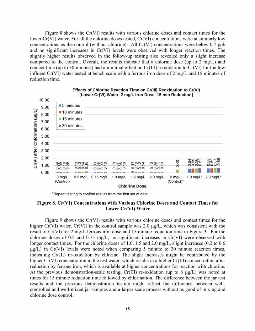
Figure 8 shows the Cr(VI) results with various chlorine doses and contact times for the lower Cr(VI) water. For all the chlorine doses tested, Cr(VI) concentrations were at similarly low concentrations as the control (without chlorine). All Cr(VI) concentrations were below 0.7 ppb and no significant increases in Cr(VI) levels were observed with longer reaction times. The slightly higher results observed in the follow-up testing also revealed only a slight increase compared to the control. Overall, the results indicate that a chlorine dose (up to 2 mg/L) and contact time (up to 30 minutes) had a minimal effect on Cr(III) reoxidation to Cr(VI) for the low influent Cr(VI) water tested at bench scale with a ferrous iron dose of 2 mg/L and 15 minutes of reduction time.

Figure 8. Cr(VI) Concentrations with Various Chlorine Doses and Contact Times for

Lower Cr(VI) Water

Figure 9 shows the Cr(VI) results with various chlorine doses and contact times for the higher Cr(VI) water. Cr(VI) in the control sample was 2.0 µg/L, which was consistent with the result of Cr(VI) for 2 mg/L ferrous iron dose and 15 minute reduction time in Figure 3. For the chlorine doses of 0.5 and 0.75 mg/L, no significant increases in Cr(VI) were observed with longer contact times. For the chlorine doses of 1.0, 1.5 and 2.0 mg/L, slight increases (0.2 to 0.6 µg/L) in Cr(VI) levels were noted when comparing 5 minute to 30 minute reaction times, indicating Cr(III) re-oxidation by chlorine. The slight increases might be contributed by the higher Cr(VI) concentration in the test water, which results in a higher Cr(III) concentration after reduction by ferrous iron, which is available at higher concentrations for reaction with chlorine. At the previous demonstration-scale testing, Cr(III) re-oxidation (up to 8 µg/L) was noted at times for 15 minute reduction time followed by chlorination. The difference between the jar test results and the previous demonstration testing might reflect the difference between well-controlled and well-mixed jar samples and a larger scale process without as good of mixing and chlorine dose control.

0.09

0.13

0.09

0.10

0.17

0.13 0.

54

0.58

0.09

0.13

0.08

0.07

0.10

0.09 0.

55

0.59

0.10

0.14

0.09

0.08

0.12

0.11 0.

40 0.56

0.61

0.09

0.16

0.10

0.10

0.14

0.13 0.

60

0.66

0.00

1.00

2.00

3.00

4.00

5.00

6.00

7.00

8.00

9.00

10.00

0 mg/L(Control)

0.5 mg/L 0.75 mg/L 1.0 mg/L 1.5 mg/L 2.0 mg/L 0 mg/L(Control)*

1.0 mg/L* 2.0 mg/L*

Cr(

VI)

aft

er

Ch

lori

nati

on

(µ

g/L

)

Chlorine Dose

Effects of Chlorine Reaction Time on Cr(III) Reoxidation to Cr(VI)[Lower Cr(VI) Water, 2 mg/L Iron Dose, 15 min Reduction]

5 minutes10 minutes15 minutes30 minutes

*Repeat testing to confirm results from the first set of data.

16

Figure 9. Cr(VI) Concentrations with Various Chlorine Doses and Contact Times for

Higher Cr(VI) Water

Evaluation of Polymer Mixing Time

The results of polymer mixing time tests for the lower Cr(VI) water are shown in Figures 9 and 10. Three mixing times were tested, including 1, 3 and 5 minutes. At the previous demonstration-scale, 0.1 mg/L polymer and a 5 minute mixing time were applied in previous research. The jar testing results showed that total Cr was effectively removed by a 1 µm filter with 0.1 mg/L polymer, regardless of the mixing time. The results suggest that the polymer mixing time could be reduced from 5 minutes to 1 minute for granular media filtration. Without polymer, total Cr concentration was between 4.4 and 7.2 µg/L in the 1 µm filtrate, indicating that particle removal was not optimal. With 0.1 µm filtration, total Cr was effectively removed with or without polymer.

The results of polymer mixing time tests for the higher Cr(VI) water are shown in Figures

12 and 13. The same trends were observed as for the lower Cr(VI) water. With 0.1 mg/L polymer, 1 µm and 0.1 µm filters effectively removed total Cr for all mixing times tested. Without polymer, only the 0.1 µm filter effectively removed total Cr. This is consistent with previous pilot findings that microfiltration can effectively remove total Cr without polymer (Blute et al. 2015a).

2.0

2.0 2.2

1.9

1.8

1.82.0

2.0 2

.3

2.0

1.9

1.92.0

2.0 2.2

2.1

2.0

2.0

2.0

2.0 2

.3

2.1 2.2 2.4

0.00

1.00

2.00

3.00

4.00

5.00

6.00

7.00

8.00

9.00

10.00

0 mg/L (Control) 0.5 mg/L 0.75 mg/L 1.0 mg/L 1.5 mg/L 2.0 mg/L

Cr(

VI)

aft

er

Ch

lori

nat

ion

(µ

g/L)

Chlorine Dose

Effects of Chlorine Reaction Time on Cr(III) Reoxidation to Cr(VI)[Higher Cr(VI) Water, 2 mg/L Iron Dose, 15 min Reduction]

5 minutes

10 minutes

15 minutes

30 minutes

17

The mixing time included one minute of rapid mix.

Figure 10. Total Cr Concentrations in 1 µm Filtered Water for the Polymer Mixing Test for Lower Cr(VI) Water

The mixing time included one minute of rapid mix.

Figure 11. Total Cr Concentrations in 0.1 µm Filtered Water for the Polymer Mixing Test for Lower Cr(VI) Water

4.4

7.2

4.5

<0.2 <0.2 <0.20.0

1.0

2.0

3.0

4.0

5.0

6.0

7.0

8.0

9.0

10.0

1 minute 3 minutes 5 minutes

Tota

l Cr

in 1

µm

Filt

rate

(µ

g/L)

Effects of Polymer Mixing Time on Total Cr Removal[Lower Cr(VI) Water, 2 mg/L Iron Dose, 15 min Reduction]

No polymer

0.1 mg/L Polymer

<0.2

0.87 0.87

<0.2 <0.2 <0.20.0

1.0

2.0

3.0

4.0

5.0

6.0

7.0

8.0

9.0

10.0


Tota

l Cr

in 0

.1 µ

m F

iltra

te (

µg/

L)

Effects of Polymer Mixing Time on Total Cr Removal[Lower Cr(VI) Water, 2 mg/L Iron Dose, 15 min Reduction]

No polymer

0.1 mg/L Polymer

18

Figure 12. Total Cr Concentrations in 1 µm Filtered Water for the Polymer Mixing Test


Figure 13. Total Cr Concentrations in 0.1 µm Filtered Water for the Polymer Mixing Test


3642 42

1.8 1.5 1.60.0

10.0

20.0

30.0

40.0

50.0

60.0

70.0

80.0

90.0

100.0


Tota

l Cr

in 1

µm

Filt

rate

(µ

g/L)

Effects of Polymer Mixing Time on Total Cr Removal[Higher Cr(VI) Water, 2 mg/L Iron Dose, 15 min Reduction]

No polymer

0.1 mg/L Polymer

1.7 1.6 1.61.9 1.0 1.70.0

10.0

20.0

30.0

40.0

50.0

60.0

70.0

80.0

90.0

100.0


Tota

l Cr

in 0

.1 µ

m F

iltra

te (

µg/

L)

Effects of Polymer Mixing Time on Total Cr Removal[Higher Cr(VI) Water, 2 mg/L Iron Dose, 15 min Reduction]

No polymer

0.1 mg/L Polymer

19

SUMMARY AND CONCLUSIONS

The jar testing results in this study showed that a ferrous iron dose of 2 mg/L and 3 mg/L provided effective Cr(VI) reduction to achieve less than 1 µg/L for the lower influent Cr(VI) water. A ferrous dose of 3 mg/L is needed for Cr(VI) reduction to below 1 µg/L for the higher Cr(VI) water. The reduction reaction between Cr(VI) and ferrous iron at 2 or 3 mg/L iron doses were found to be complete in one minute. Thus, the reduction time could be reduced significantly from the times previously tested (15, 30 and 45 minutes) as long as mixing is good and particle buildup is sufficient for effective total Cr filtration.

At bench scale, a chlorine dose up to 2 mg/L (resulting in a chlorine residual of 2 mg/L)

with a contact time up to 30 minutes did not result in significant Cr(III) re-oxidation to Cr(VI) for the lower Cr(VI) water. For the higher Cr(VI) water, slight increases in Cr(VI) concentration were noted for chlorine doses of 1.0, 1.5 and 2.0 mg/L with 30 minutes, indicating Cr(III) reoxidation by chlorine. By comparison, significant Cr(III) re-oxidation was noted in some data points at the previous demonstration testing with a higher influent Cr(VI) water (approximately 100 µg/L) (Blute et al, 2015b). The discrepancy might be caused by the difference of well-controlled bench scale and a larger demonstration scale. Consequently, demonstration-scale testing was conducted in this study, which is documented in the following chapters.

The bench-scale polymer mixing test confirmed that polymer was necessary for effective

total Cr removal by granular media filter (represented by 1 µm filter) and not necessary for microfiltration (represented by 0.1 µm filter). The bench results also suggest the polymer mixing time may not have a strong impact on total Cr removal by either 1 µm or 0.1 µm filters. Therefore, the polymer mixing tank size might be reduced to save footprint. Note that polymer contact time was not further tested in the demonstration testing as it would have introduced another variable in addition to reduction times and ferrous iron doses that were the primary focus of this study.

20

CHAPTER 5. DEMONSTRATION TESTING OF RCF REDUCTION TIME AND IRON DOSE

Based on the jar testing results in Chapter 4, demonstration-scale testing was conducted to further evaluate the impacts of reduction time and iron dose on RCF effectiveness for Cr(VI) removal. This chapter summarizes the demonstration-scale testing conducted with a progressive cavity pump that was already part of the RCF process at Glendale. Additional demonstration testing was conducted with a centrifugal pump, which is presented in Chapter 6.

OBJECTIVES

The objectives of the demonstration testing described this chapter included: Assessing the relationship observed in jar testing between iron dose and reduction

times at demonstration scale, Evaluating the effectiveness of inline chlorine injection for ferrous iron oxidation

and impact on Cr(III) re-oxidation, and Evaluating the consistency of process performance for Cr(VI) and total Cr

removal.


This section summarizes the raw water quality and the operational conditions tested at the demonstration-scale.

Raw Water Quality

A lower Cr(VI) water was tested in the demonstration facility to reflect levels commonly observed by utilities needing Cr(VI) treatment for the MCL compliance. The raw water quality during the demonstration testing period is summarized in Table 8. Cr(VI) was in the range of 13 - 18 µg/L with an average of 14.1 µg/L. Total Cr was in the range of 12 -15 µg/L with an average of 12.7 µg/L. The water quality was similar to the lower Cr(VI) water used for jar testing. Table 8. Raw Water Quality for Demonstration Testing with the Progressive Cavity Pump

Parameter (Unit) Average Range Cr(VI) (µg/L) 14.1 13 – 18 Cr, Total (µg/L) 12.7 12 – 15 pH (- ) 7.7 7.2 - 7.9 Turbidity (NTU) 0.20 0.01 - 0.32 Iron, Total, field (mg/L) 0.01 <0.02 - 0.15

21

RCF Process

Figure 14 provides a schematic of the demonstration RCF process evaluated in this study. The RCF process was operated at its design capacity of 100 gpm. Ferrous sulfate was injected through a static mixer into the raw water pipeline. Three reduction times were evaluated in this study, including 15, 5 and 1 minute. For 15 and 5 minutes, one 1,500-gallon tank and one 500-gallon tank were used as the reduction tank, respectively. For 1 minute reduction time, the reduction tank was bypassed with a 2-inch hose, which provided approximately 1 minute of contact time. Sodium hypochlorite was injected through a static mixer into the pipeline (without a chlorine contact tank as had been used in previous demonstration testing). Polymer was added to the rapid mix tank downstream, which provided a 5-minute contact time. Water was pumped from the progressive cavity pump to a granular media filter (2 feet of anthracite and 1 feet of sand) to remove ferric/chromium particles. Two filters were alternated (one in duty and one in standby or backwash cycle). The progressive cavity pump was part of the original design to minimize particle breakdown (Blute et al. 2013; Blute et al. 2015b). The effects of a different pump type (centrifugal pump) on RCF effectiveness for chromium removal was evaluated after this testing and is documented in Chapter 6.

Figure 14. Schematic of RCF Process Evaluated with a Progressive Cavity Pump

Operational Conditions

Based on the jar testing results, two ferrous iron doses and three reduction times were selected for this demonstration testing (Table 9). A total of six runs were conducted, with each run lasting approximately one week. The chlorine dose was adjusted based on the ferrous iron dose and reduction time to achieve a target chlorine residual concentration of 0.2 – 0.4 mg/L at the post chlorination location. The polymer dose was 0.1 mg/L as active polymer for all runs. The filters were operated with 24 hour run cycles for all the conditions tested, as previous demonstration testing indicated that effective filter backwash is critical for chromium removal (Blute et al., 2015b). At least five filter run cycles were evaluated for each operational condition.

22

Table 9. Operational Conditions of Demonstration RCF with Progressive Cavity Pump

Run No.

Ferrous Iron Dose

Target Reduction

Time Chlorine

Residual Target Polymer

Dose*

Filter Backwash Frequency Test Period

1 3 mg/L 15 minutes 0.2 – 0.4 mg/L 0.1 mg/L Every 24 hours

8/15/2014 - 10/21/2014^


12/12/2014 - 12/18/2014


12/19/2014 - 12/29/2014


12/30/2014 - 1/4/2015


1/5/2015 - 1/11/2015


1/12/2015 - 1/17/2015

*As active polymer ^Including some system offline period

Sampling and Monitoring

Table 10 summarizes the RCF sampling and analysis frequencies for demonstration testing. Cr(VI) and total Cr were monitored as paired samples in raw water, the rapid mix tank effluent, and the filter effluent. Cr(VI) was also monitored at post-reduction and post chlorination points to evaluate the change of Cr(VI) after reactions with ferrous iron and potential Cr(III) re-oxidation by chlorine. Total and ferrous iron were monitored to verify iron dose, ferrous oxidation by chlorination and total iron removal by the granular media filters. pH and turbidity were also monitored throughout the process. In addition, bacteria (total coliform, E. Coli, and HPC) were monitored three times a week as recommended by DDW due to positive Bacti noted in a previous RCF study.

23

Table 10. Sampling and Analysis for Demonstration RCF with a Progressive Cavity Pump Analyte Lab or

Field Raw Water (SP-001)

Raw Water with Ferrous (SP-100)

Post-Reduction (SP-103)

Post Chlorina-tion

Rapid Mix Tank Effluent (SP-203)

Post-Filtration (SP-301 or SP-302)

Bacti Lab 3/W N/A N/A N/A 3/W 3/W Cr(VI) Lab 1/D N/A 1/D 1/D 1/D 1/D Cr(VI) Field N/A N/A 1/D N/A N/A N/A Total Cr Lab 1/D N/A N/A N/A 1/D 1/D Free Chlorine Field N/A N/A N/A 2/D 2/D 2/D Iron, Ferrous Field N/A 1/D 2/D 2/D 2/D 2/D Iron, Total Lab N/A N/A 1/D 2/D 1/D 1/D Iron, Total Field 1/D 1/D 2/D 1/D 2/D 2/D HPC Lab 3/W N/A N/A N/A 3/W 3/W pH Field 1/D 1/D 1/D 1/D 1/D 1/D Turbidity Field 1/D 1/D 1/D 1/D 1/D 1/D 3/W – Three times per week; 1/D – Daily; 2/D – Twice a day, one in the morning, one in the afternoon N/A – Not analyzed

Analytical Methods

The field and lab analytical methods used in this demonstration study are summarized in Table 11. For total Cr analysis, all RCF filter effluent samples were analyzed with digestion as a previous study found significant carbon interference at low µg/L levels (Blute et al., 2015a). The other total Cr samples were analyzed without digestion as total Cr was expected to be well above 5 µg/L.

Table 11. Analytical Methods

Analyte Analytical Method Method Reporting Limit Bacti (COLI10) SM 9221B 1.1 MPN/100mL Cr(VI), Field Hach Method 8023 10 µg/L Cr(VI), Lab EPA 218.6 0.02 µg/L Total Cr EPA 200.8 1 µg/L without digestion; 0.2 µg/L

with digestion Free Chlorine Hach Method 8021 0.02 mg/L Iron, Ferrous Hach Method 8146 0.02 mg/L Iron, Total Hach Method 8008 0 mg/L Iron, Total EPA 200.7 0.05 mg/L HPC SM 9215B 1 CFU/mL pH SM 4500H+ B N/A Turbidity SM 2130B / Hach 2100Q 0.02 NTU

EPA - United States Environmental Protection Agency; SM - Standard Methods N/A - not applicable.

24

RESULTS

This section summarizes the results of the demonstration RCF testing with the progressive cavity pump.

Cr(VI) Reduction by Ferrous Iron

Cr(VI) concentrations at the post reduction location (SP-103) are summarized in Table 12 and Figure 15. A combination ferrous dose of 3 mg/L and 15 or 5 minutes’ reduction time effectively reduced Cr(VI) to below 1 µg/L Cr(VI). However, with a ferrous dose of 3 mg/L and 1 minute reduction, Cr(VI) concentrations were between 1.1 and 2.3 µg/L, suggesting incomplete Cr(VI) reduction by ferrous iron in such a short contact time. For a ferrous dose of 2 mg/L and 15 minutes, Cr(VI) concentrations were all below 1 µg/L. When reduction time decreased to 5 minutes, Cr(VI) levels increased to 0.47 – 1.6 µg/L. With 1 minute reduction time, Cr(VI) concentrations were between 3.4 and 5.5 µg/L, significantly higher than the other conditions tested. Overall, a combination of ferrous dose of 2 or 3 mg/L with a reduction time of 5 or 15 minutes was effective for Cr(VI) reduction to below or close to 1 µg/L.

Table 12. Cr(VI) at Post Reduction for Demonstration RCF with Progressive Cavity Pump

Run No.

Ferrous Iron Dose Target

(mg/L) Reduction Time

(minute)

Average Cr(VI) at Post Reduction

(µg/L)

Range of Cr(VI) at Post Reduction

(µg/L) 1 3 15 0.09 <0.02 – 0.19 2 3 5 0.13 <0.02 – 0.49 3 3 1 1.9 1.1 – 2.3 4 2 15 0.53 0.46 – 0.59 5 2 5 1.0 0.47 – 1.60 6 2 1 5.0 3.4 – 5.5

25

Figure 15. Cr(VI) Results at Post Reduction for Demonstration RCF with Progressive

Cavity Pump

Ferrous Iron Oxidation by Chlorine

Ferrous iron concentrations at the post reduction and post rapid mix tank locations are summarized in Table 13. Ferrous iron concentrations at the post reduction location varied with the ferrous iron dose as well as the reduction time. The chlorine dose was adjusted according to the ferrous concentration. Ferrous iron was non-detect (<0.02 mg/L) to 0.04 mg/L in the rapid mix tank effluent, indicating effective ferrous iron oxidation by chlorine.

Table 13. Chlorine Dose and Residuals for Demonstration RCF with a Progressive Cavity

Pump

Run No.

Ferrous Iron Dose

Target (mg/L)

Reduction Time

(minute)

Average and Range of

Ferrous Iron in Reduction

Effluent (mg/L) Chlorine Dose

(mg/L)

Average and Range of Chlorine Residual (mg/L)


Ferrous Iron in Rapid Mix Tank Effluent

(mg/L)

1 3 15 1.60 (0.69 – 1.95) ~1.97

0.35 (0.14 – 0.60)

<0.02 (<0.02 – 0.03)

2 3 5 1.46 (0.73 – 1.95) ~1.89

0.30 (0.18 – 0.45)

<0.02 (<0.02 – 0.02)

3 3 1 1.79 (1.40– 2.29) ~2.04

0.33 (0.10– 0.70)

<0.02 (<0.02)

4 2 15 1.14 (0.69 – 1.38) ~1.43

0.33 (0.15 – 0.55)

<0.02 (<0.02 – 0.02)

0.1

2

<0.0

2

2.1

0.5

8

0.4

7

5.2

0.0

98

<0.0

2 1.1

0.4

6 1.2

5.1

0.0

9

0.0

88

2.3

0.5

4 1.2

3.4

0.0

24

0.1

6

1.9

0.5

9 1.6

5.2

0.0

76

<0.0

2

2.2

0.4

9

0.5

4

5.5

0.1

9

0.4

9 1.9

1.1

5.3

0.0

79

1.1

<0.0

2

0

2

4

6

8

10

12

14

16

18

20

Run 1 Run 2 Run 3 Run 4 Run 5 Run 6

He

xava

len

t C

hro

miu

m (

µg/

L)

26

Run No.

Ferrous Iron Dose

Target (mg/L)

Reduction Time

(minute)




(mg/L)




(mg/L)

5 2 5 1.26 (1.13 – 1.38) ~1.31

0.36 (0.25 – 0.58)

<0.02 (<0.02 – 0.03)

6 2 1 1.27 (0.32 – 1.7) ~1.46

0.43 (0.1 – 1.78)

<0.02 (<0.02 – 0.04)

Figure 16 shows chlorine residual concentrations at the post chlorination location. The

chlorine feed system was manually operated in this study (i.e. not flow paced). The chlorine pump rate was adjusted daily based on the monitored ferrous iron concentration at the post reduction location and the chlorine residual at the post chlorination location. The chlorine residual target was 0.2 - 0.4 mg/L. The average chlorine residual of each run were in the range of 0.30 – 0.43 mg/L. Most chlorine residuals were below 0.4 mg/L, except several occasions.

Figure 16. Chlorine Residual at Post Chlorination for Demonstration RCF with

Progressive Cavity Pump

0.0

0.2

0.4

0.6

0.8

1.0

1.2

1.4

1.6

1.8

2.0


Ch

lori

ne

Res

idu

al (

mg/

L)


27

Cr(III) Re-oxidation

Cr(III) re-oxidation to Cr(VI) was evaluated by comparing average Cr(VI) concentrations at different locations in the treatment process as shown in Table 14 and Figure 17. In Runs 1, 2, 4 and 5, Cr(VI) concentrations slightly increased as post reduction water passed through chlorination, rapid mix, and granular media filtration processes. The Cr(VI) concentration differences between filter effluent and post reduction were less than 1.5 µg/L, indicating slight Cr(III) re-oxidation to Cr(VI). In the jar tests, a reduction time of 15 minutes was tested for Cr(III) re-oxidation by chlorine (Figure 8). The jar testing results suggest little Cr(III) re-oxidation with a chlorine dose up to 2 mg/L and contact time up to 30 minutes for the lower Cr(VI) water. The demonstration results of Runs 1 and 4 are generally consistent with the jar testing findings.

In Runs 3 and 6, Cr(VI) concentrations increased much more significantly than in the

other runs. The differences between the average filter effluent concentration and average post reduction concentration were up to 4.8 µg/L. These results suggest considerable Cr(III) re-oxidation by chlorine with a shorter reduction time, even though chlorine doses and residual concentrations were similar to the other runs. The demonstration results suggest that 1 minute is not sufficient for complete Cr(VI) reduction at demonstration-scale.

Table 14. Average Cr(VI) Concentrations of Individual Monitoring Locations of Each Run

Run No.

Ferrous Iron Dose

Target (mg/L)

Reduction Time

(minutes)

Post Reduction

(µg/L)

Post Chlorination

(µg/L)

Rapid Mix Tank

Effluent (µg/L)

Filter Effluent (µg/L)

1 3 15 0.09 0.76 0.77 1.40 2 3 5 0.13 1.09 1.10 1.50 3 3 1 1.90 6.20 5.80 6.00 4 2 15 0.53 1.10 1.14 1.50 5 2 5 1.00 1.90 1.90 2.30 6 2 1 5.00 9.50 9.50 9.80

28

Figure 17. Average Cr(VI) Concentrations of Individual Monitoring Locations of Each

Run Note: The bars represent the range of Cr(VI) concentrations, i.e. the maximum and minimum of each location of each run.

Cr(VI) and Total Cr Removal

Cr(VI) and total Cr removal by filtration is shown in Figures 18 and 19, respectively. Cr(VI) concentrations are similar to total Cr concentrations in all the runs (except one data point in Run 1), indicating that Cr(III) particles were effectively removed by filtration and Cr(VI) was the dominant chromium species in the filtered water. In Runs 1, 2, 4 and 5, both Cr(VI) and total Cr were below 3 ppb (except one data point in Run 1), indicating effective removal by filtration. In Runs 3 and 6, much higher Cr(VI) and total Cr concentrations were observed in the filtered water, which were carried over from the pre-treatment process before filtration.

0

2

4

6

8

10

12

14

16

18

20


Hex

aval

en

t C

hro

miu

m (

µg/

L)

Post Reduction Post Chlorination Rapid Mix Tank Effluent Filter Effluent

29

Figure 18. Cr(VI) Concentrations in Filter Effluent

Figure 19. Total Cr Concentrations in Filter Effluent


The RCF demonstration testing with a progressive cavity pump suggest that a ferrous dose of 2 or 3 mg/L with a reduction time of 5 or 15 minutes was effective for Cr(VI) reduction to below or close to 1 µg/L (Runs 1, 2, 4 and 5). Chlorine effectively oxidized ferrous iron with a chlorine dose of 0.2 – 0.4 mg/L. Minor Cr(III) re-oxidation to Cr(VI) by chlorine (< 1.5 µg/L) was observed for the test runs with reduction times of 5 or 15 minutes. Cr(III) particles were

1.7

1.4

7.5

1.3 1.7

10

0.8

5

1.6

7.3

1.6 2

.3

9.8

1.5

1.5

0.0

46 1.6 2

.5

9.6

1.4 1.6

6.8

1.5

2.8

9.7

1.2 1.6

7.4

1.6 1.9

10

0.9

2

1.4

6.8

2.4

9.6

1.6

2.7

2.2

0

2

4

6

8

10

12

14

16

18

20


He

xava

len

t C

hro

miu

m (

µg/

L)

4.8

2.5

8.0

1.6 2.0

11

1.1 2

.1

7.4

1.6 2

.1

9.9

1.7 2.1

0.3

8 1.8 2

.6

10

0.9

3 1.8

6.7

1.7 2

.6

9.6

1.6 1.8

8.4

1.9 2

.4

10

1.6

1.6

7.8

2.9

10

1.5

3.0

2.9

0

2

4

6

8

10

12

14

16

18

20


Tota

l Ch

rom

ium

(µ

g/L)

30

effectively removed by granular media filtration. Cr(VI) and total Cr in the filtered water were below 3 µg/L, except one data point.

Comparatively, a reduction time of 1 minute was not sufficient for complete Cr(VI)

reduction by a ferrous iron dose of 2 or 3 mg/L (Runs 3 and 6). More significant Cr(III) re-oxidation to Cr(VI) by chlorine was also observed in these runs (up to 4.8 µg/L), although chlorine doses and residual levels were similar as in the other runs. Consequently, Cr(VI) and total Cr in the filtered water were much higher than in the other runs (up to 11 µg/L). The results indicate that reduction time plays a key role in Cr(VI) reaction with ferrous iron and Cr(III) re-oxidation by chlorine, when chlorine residuals were maintained below approximately 0.5 mg/L.

31

CHAPTER 6. DEMONSTRATION-SCALE TESTING OF RCF ALTERNATIVE PUMPING

Progressive cavity pumping was originally specified for the RCF treatment process in the desire to minimize floc breakup before the filters. Cost estimates suggested that significant cost savings could be realized if a more common pump type, a centrifugal pump, is used instead of a progressive cavity pump. However, no comparison of the pumps had previously been performed. The same demonstration RCF treatment process as described in Chapter 5 was tested using a centrifugal pump in place of the progressive cavity pump to evaluate Cr(VI) and total Cr removal at iron doses and reduction times found effective in Chapter 5. This chapter summarizes the testing results of RCF with a centrifugal pump.

OBJECTIVES

The objectives of the demonstration-scale testing included: Evaluating the effects of centrifugal pumping on RCF performance for chromium

removal in comparison with RCF with progressive cavity pumping, Confirming the iron doses and reduction times found effective in Chapter 5, and Confirming the effectiveness of inline chlorine injection for ferrous iron oxidation

and impact on Cr(III) reoxidation.


This section summarizes the raw water quality and the operational conditions tested.

Raw Water Quality

The same water source as described in Chapter 5 was tested for RCF with centrifugal pumping. The raw water quality during this demonstration testing period is summarized in Table 15. Cr(VI) was in the range of 14 - 16 µg/L with an average of 14.6 µg/L. Total Cr was in the same range, with an average of 14.7 µg/L.

Table 15. Raw Water Quality for Demonstration Testing with Centrifugal Pumping

Parameter (Unit) Average Range Cr(VI) (µg/L) 14.6 14 - 16 Cr, Total (µg/L) 14.7 14 - 16 pH (- ) 7.7 7.2 - 7.9 Turbidity (NTU) 0.21 0.01 – 0.32 Iron, Total, field (mg/L) 0.01 <0.02 - 0.15

32

RCF Process

The same RCF process as described in Chapter 5 was tested, except a centrifugal pump was used in place of the progressive cavity pump (Figure 20).

Figure 20. RCF Process Schematic with a Centrifugal Pump

Operational Conditions

Based on the demonstration results with progressive cavity pumping, two ferrous iron doses and two reduction times were selected for the demonstration testing with centrifugal pumping (Table 16). A total of four runs were conducted, with each run lasting approximately one week. The other operational conditions (chlorine residual target, polymer dose and filter backwash) were kept the same as the demonstration testing with progressive cavity pumping to allow comparison. At least five filter run cycles were evaluated for each operational condition.

Table 16. Operational Conditions of Demonstration RCF with Centrifugal Pumping

Run No.

Ferrous Iron Dose

Target Reduction

Time Chlorine

Residual Target Polymer

Dose*

Filter Backwash Frequency Test Period


2/2/15 - 2/13/15


2/16/15 - 2/20/15


2/24/15 - 2/28/15


3/2/15 - 3/11/15

*As active polymer

33

Sampling and Monitoring

The same sampling and monitoring frequency was applied as in the demonstration testing with progressive cavity pumping (Table 10).

Analytical Methods

The same analytical methods were applied as in the demonstration testing with progressive cavity pumping (Table 11).

RESULTS

This section summarizes the results of the demonstration RCF testing with progressive cavity pumping.

Cr(VI) Reduction by Ferrous Iron

Cr(VI) concentrations at the post reduction location (SP-103) are summarized in Table 17 and Figure 21. With a ferrous iron dose of 3 mg/L and a 15-minute reduction time, Cr(VI) concentrations at SP-103 were below 1 µg/L. With the same ferrous iron dose and 5-minute reduction time, Cr(VI) concentrations were in the range of 0.22 – 0.62 µg/L. When the ferrous iron dose was reduced to 2 mg/L, Cr(VI) concentrations were between 1.7 and 2.1 µg/L with 15-minute reduction time and between 1.1 and 1.3 µg/L with 5-minute reduction time. These Cr(VI) results are generally consistent with the progressive cavity pumping test results (Table 11) but with some variation. The differences might be a result of re-arrangement of the reduction tank(s) to enable a parallel study of RCF with membrane filtration, and/or variations in operations. Overall, the results indicate effective Cr(VI) reduction by ferrous iron for the four conditions tested.

Table 17. Cr(VI) at Post Reduction for Demonstration RCF with Centrifugal Pumping

Run No.

Ferrous Iron Dose Target

(mg/L) Reduction Time

(minute)

Average Cr(VI) at Post Reduction

(µg/L)

Range of Cr(VI) at Post Reduction

(µg/L) 1 3 15 0.66 <0.02 – 0.91 2 2 15 1.9 1.7 – 2.1 3 2 5 1.2 1.1 – 1.3 4 3 5 0.39 0.22 – 0.62

34

Figure 21. Cr(VI) Results at Post Reduction for Demonstration RCF with a Centrifugal

Pump

Ferrous Iron Oxidation by Chlorine

Ferrous iron concentrations at post reduction and post rapid mix tank locations are summarized in Table 18. The ferrous iron results are consistent with the results for the progressive cavity pump tests (Table 13). The chlorine dose was adjusted according to the ferrous concentration at the post reduction location. Ferrous iron was non-detect (<0.02 mg/L) to 0.04 mg/L in the rapid mix tank effluent, indicating effective ferrous iron oxidation by chlorine.

Table 18. Chlorine Dose and Residuals for Demonstration RCF with Centrifugal Pumping

Run No.

Ferrous Iron Dose

Target (mg/L)

Reduction Time

(minute)




(mg/L)




(mg/L)

1 3 15 1.44 (1.0 – 1.79) ~1.54

0.27 (0.02 – 0.78)

<0.02 (<0.02)

2 2 15 0.89 (0.52 – 1.23) ~1.43

0.33 (0.11 – 0.55)

<0.02 (<0.02)

3 2 5 0.98 (0.38– 1.44) ~1.27

0.31 (0.20– 0.69)

<0.02 (<0.02 – 0.04)

4 3 5 1.28 (0.11 – 1.71) ~1.92

0.19 (0.07 – 0.41)

<0.02 (<0.02 – 0.03)

0.3

8 1.7

1.1

0.5

5

0.9

1 1.9

1.2

0.4

1

0.7

7 1.9

1.3

0.6

2

0.9

2.0

1.2

0.2

8

1.0

2.1

1.2

0.2

6

<0.0

2

0.2

2

0

2

4

6

8

10

12

14

16

18

20

Run 1 Run 2 Run 3 Run 4

He

xava

len

t C

hro

miu

m (

µg/

L)

35

The chlorine residual concentrations at the post chlorination location are shown in Figure 22. The average chlorine residual of each run were in the range of 0.19 – 0.33 mg/L. Most chlorine residuals were below 0.4 mg/L (within the target residual range), except on several occasions.

Figure 22. Chlorine Residual at Post Chlorination for Demonstration RCF with

Centrifugal Pumping

Cr(III) Re-oxidation

Similar to the progressive cavity pumping tests, Cr(III) re-oxidation to Cr(VI) was evaluated by comparing average Cr(VI) concentrations at different locations in the treatment process as shown in Table 19 and Figure 23. In Runs 1, 3 and 4, Cr(VI) concentrations increased gradually through the treatment processes (from post reduction to filtration) by a maximum of 1.3 µg/L. In Run 2, Cr(VI) concentrations at the post reduction location were higher than the other monitoring locations for unknown reasons. Overall, the results suggest slight Cr(VI) re-oxidation to Cr(VI) by chlorine under these conditions, which are in agreement with the progressive cavity pump testing results (Figure 17 and Table 14).

Table 19. Average Cr(VI) Concentrations of Individual Monitoring Locations of Each Run

Run No.

Ferrous Iron Dose

Target (mg/L)

Reduction Time

(minutes)

Post Reduction

(µg/L)

Post Chlorination

(µg/L)

Rapid Mix Tank

Effluent (µg/L)

Filter Effluent (µg/L)

1 3 15 0.66 0.6 0.63 1.0 2 2 15 1.9 0.8 0.8 1.3 3 2 5 1.2 1.8 2.0 2.5 4 3 5 0.4 1.2 1.1 1.7

0.0

0.2

0.4

0.6

0.8

1.0

1.2

1.4

1.6

1.8

2.0

Ch

lori

ne

Re

sid

ual

(m

g/L)


36

Figure 23. Average Cr(VI) Concentrations of Individual Monitoring Locations of Each

Run Note: The bars represent the range of Cr(VI) concentrations, i.e. the maximum and minimum of each location of each run.

Cr(VI) and Total Cr Removal

Cr(VI) and total Cr concentrations in the filter effluent are shown in Figures 24 and 25, respectively. Cr(VI) concentrations are similar to total Cr concentrations in all the runs, indicating that the primary species in filtered water was Cr(VI). Thus, Cr(III) particles were effectively removed by filtration using a centrifugal pump before the filter. In all the runs, both Cr(VI) and total Cr concentrations were below 3 µg/L, which are similar to the progressive cavity pumping test results. Progressive cavity pumping was originally specified for the RCF treatment process in the desire to minimize floc breakup before the filters. However, the results with centrifugal pumping indicate effective particle removal by granular media filtration. These findings support the concept of using centrifugal pumping in place of progressive cavity pumping for cost savings.

0

2

4

6

8

10

12

14

16

18

20


He

xava

len

t C

hro

miu

m (

µg/

L)

Post Reduction Post Chlorination Rapid Mix Tank Effluent Filter Effluent

37

Figure 24. Cr(VI) Concentrations in Filter Effluent

Figure 25. Total Cr Concentrations in Filter Effluent


The demonstration test results with centrifugal pumping confirm that a ferrous dose of 2 or 3 mg/L with a reduction time of 5 or 15 minutes were effective for Cr(VI) reduction to below 3 µg/L. Chlorine injected inline effectively oxidized ferrous iron remaining at post reduction. Slight Cr(III) re-oxidation to Cr(VI) by chlorine (< 1.3 µg/L) was observed. Cr(III) particles were effectively removed by granular media filtration with centrifugal pumping and the filtered Cr(VI) and total Cr concentrations were below 3 µg/L. The results are similar to the results for the progressive cavity pumping tests, suggesting that centrifugal pumping could replace progressive cavity pumping for cost savings.

1.5

1.5 2

.3

1.9

0.8

4

1.4

2.6

1.6

0.9

2

1.2

2.5

2.1

0.8

2

1.1

2.7

1.6

0.8

6

1.3 2

.4

1.4

1.2 1.7

0

2

4

6

8

10

12

14

16

18

20


He

xava

len

t C

hro

miu

m (

µg/

L)

1.3 1.5 2

.5

2.1

0.9

5

1.5

2.7

1.9

0.9

1

1.3

2.5

2.4

0.9

5

1.2

2.7

2.4

0.9

9

1.4 2

.4 2.8

1.2 2

.3

0

2

4

6

8

10

12

14

16

18

20


Tota

l Ch

rom

ium

(µ

g/L)

38

CHAPTER 7. COST ANALYSIS

Cr(VI) treatment costs were developed for WBA and RCF in the previous study by the City of Glendale (Blute et al., 2013) and updated in Water Research Foundation (WRF) Report #4423 (Blute et al., 2015b). In this study, RCF costs were further updated based on the findings from the demonstration testing described in Chapters 5 and 6. WBA costs in WRF #4423 were updated to 2015 dollars to provide a direct comparison with RCF. In addition, SBA cost estimates were developed using the same methodology as for the prior RCF and WBA technologies (Blute et al., 2013). This chapter summarizes the treatment costs for RCF, SBA and WBA, including capital, annual O&M and 20-year net present value (NPV). Detailed costs are provided in Appendix A.

METHODOLOGY

The capital and O&M costs were developed using the approach illustrated in Figure 26, which is the same approach as used in previous studies (Blute et al., 2013 and 2015b). The capital cost factors and engineering factors are summarized in Table 20, respectively. Details are described in the report published by the City of Glendale (Blute et al., 2013).

Previous RCF and WBA costs were developed for three flow rates, 100 gpm, 500 gpm

and 2,000 gpm. In this study, RCF and WBA costs were estimated for 1,000 gpm to add this flow rate. SBA costs were developed for all four flow rates. All previous costs are adjusted from to 2015 dollars using Engineering News-Record (ENR) indices for Los Angeles, California.

The expected level of accuracy for the cost estimates presented in this chapter is

classified by the Association for the Advancement of Cost Engineering International (AACE) as an International Class 5 estimate. Typical uses for Class 5 estimates include assessment of initial viability, evaluation of treatment trains, and long range capital planning. Accuracy ranges for Class 5 estimates are -20% to -50% on the low side, and +30% to +100% on the high side. A typical rate of -30% to +50% was applied to the cost estimates in this report to demonstrate the accuracy range of estimates.

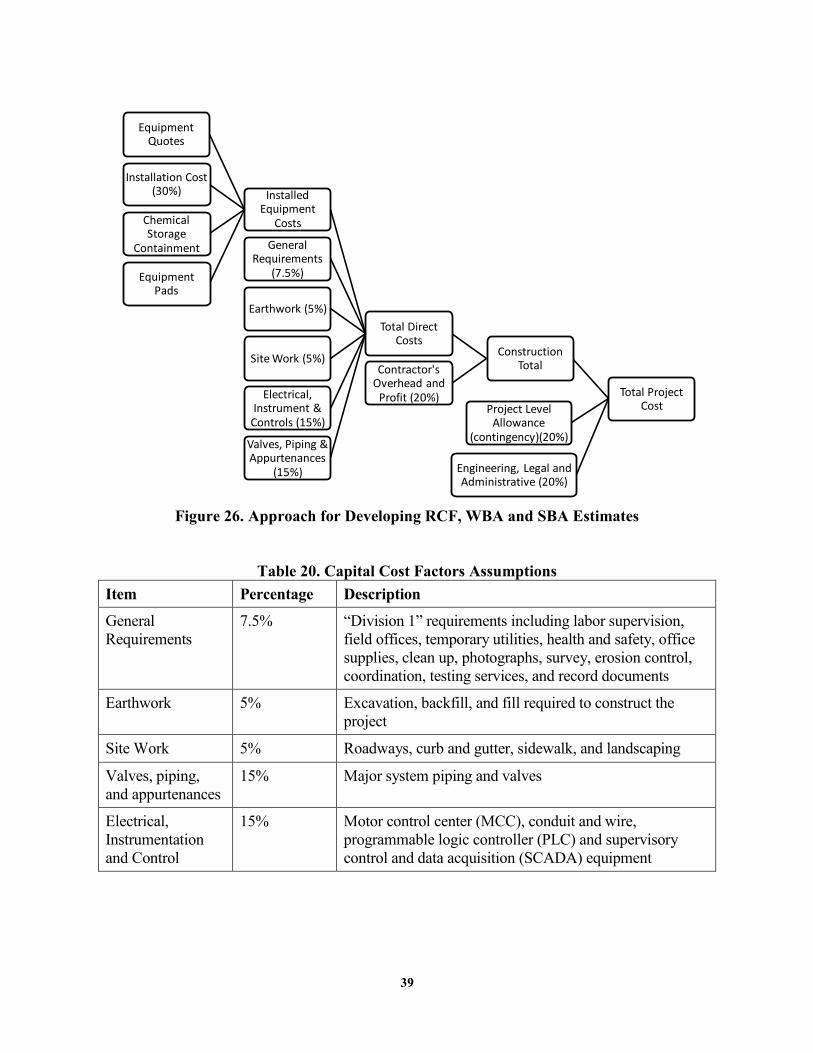
39

Figure 26. Approach for Developing RCF, WBA and SBA Estimates

Table 20. Capital Cost Factors Assumptions Item Percentage Description

General Requirements

7.5% “Division 1” requirements including labor supervision, field offices, temporary utilities, health and safety, office supplies, clean up, photographs, survey, erosion control, coordination, testing services, and record documents

Earthwork 5% Excavation, backfill, and fill required to construct the project

Site Work 5% Roadways, curb and gutter, sidewalk, and landscaping

Valves, piping, and appurtenances

15% Major system piping and valves

Electrical, Instrumentation and Control

15% Motor control center (MCC), conduit and wire, programmable logic controller (PLC) and supervisory control and data acquisition (SCADA) equipment

Total Project Cost

Engineering, Legal and Administrative (20%)

Project Level Allowance

(contingency)(20%)

Construction Total

Total Direct Costs

Installed Equipment

Costs

Equipment Quotes

Installation Cost (30%)

Chemical Storage

Containment

Equipment Pads

General Requirements

(7.5%)

Earthwork (5%)

Site Work (5%)

Electrical, Instrument &

Controls (15%)

Valves, Piping & Appurtenances

(15%)

Contractor's Overhead and

Profit (20%)

40

Table 21. Engineering Factors Assumptions Item Percentage Description

Contractor’s Overhead and Profit

20% Includes bonds, mobilization and demobilization, insurance, overhead and profit, and management reserves

Project Level Allowance 20% Budget item to cover change orders due to unforeseen conditions

Engineering, Legal and Administrative

20% Includes permits, legal fees, and engineering fees for design and construction.

DESIGN WATER QUALITY

The same design water quality used in the previous cost estimates (Blute et al., 2013) was used in this cost update (Table 22) to provide a direct comparison with the prior estimates. The design concentrations were selected based on Glendale water quality and groundwater quality for several nearby Southern California cities. The ways in which water quality variations might impact the costs are as follows:

Cr(VI) concentrations: Raw water Cr(VI) concentration is not considered to

affect RCF capital or O&M costs, as research has shown that a fixed ferrous sulfate dose can effectively removal a range of Cr(VI) concentrations (from 15 µg/L to 100 µg/L). WBA resin life (part of O&M cost) is likely affected by raw water Cr(VI) concentrations. The assumed Cr(VI) concentration of 50 µg/L is a relatively conservative assumption for most agencies.

pH, alkalinity and calcium concentrations: These levels can affect the sizing and costs for pre- and post-pH adjustment systems of WBA. The average concentrations were input into the Tetra Tech RTW model to estimate the quantity of acid or CO2 required to adjust the pH to 6.0 prior to WBA. Note that the sizing and costs of pH adjustment systems would vary for water systems with different pH, alkalinity, and calcium concentrations.

Sulfate concentrations: Sulfate is a key water quality parameter that affects SBA resin life between regenerations. A higher sulfate concentration typically results in a shorter SBA resin life, thus requiring more frequent regenerations. Two sulfate concentrations were used for cost estimates, 50 mg/L and 110 mg/L. 50 mg/L is a relatively moderate sulfate concentration, while 110 mg/L is a high sulfate concentration (observed in Glendale’s groundwater).

41

Table 22. Design Raw Water Quality for RCF, WBA and SBA Parameter (unit) Design Value

Cr(VI) (µg/L) 50

pH (pH units) 7.3

Alkalinity (mg/L as CaCO3) 191

Calcium (mg/L as Ca) 79

Sulfate (mg/L) 50 and 110

RCF

The RCF capital and O&M costs were initially developed in Blute et al. (2013) and updated in Blute et al. (2015b) for 100 gpm, 500 gpm, and 2,000 gpm systems. These capital and O&M costs were further updated based on the results of this study. Capital and O&M costs were also developed for a 1,000 gpm system.

Figure 27 illustrates the optimized RCF process, for which the capital and O&M costs

were updated/developed. The RCF process consisted of ferrous iron injection (2 mg/L ferrous iron dose), 5-minutes reduction, inline chlorination for excess ferrous ion oxidation, polymer addition and granular media filtration. Centrifugal pumping was used instead of progressive cavity pumping. For this study, the costs were developed based on granular media filtration; microfiltration is an alternative filtration approach. The spent filter backwash water can be treated by settling/dewatering and then recycled back to the treatment process. The dewatered solids can be disposed to an appropriate landfill. Alternatively, the spent filter backwash water can be discharged directly to the sewer if the water quality and quantity meet the requirements for sewer discharge. Costs were developed for both scenarios (with and without recycle).

42

The highlighted area represents the optional spent filter backwash water treatment for recycle.

Figure 27. RCF Process Flow Diagram The design criteria used for estimating RCF costs are summarized in Table 23. Based on

the demonstration-scale RCF results in this study, a fixed ferrous iron dose of 2 mg/L and 5-minutes reduction time were assumed. Inline chlorination with a chlorine residual target of 0.2 mg/L was assumed for excess ferrous iron oxidation. A chlorine dose of 1.3 mg/L was assumed based on the chlorine dose used in this study. The filter run cycle was assumed to be 24 hours as tested in this study. The other design criteria remain the same as for the previous cost estimates.

INFLUENT

GN-3

STATIC MIXER

FERROUS SULFATE

STORAGE & HANDLING SYSTEM

POLYMER STORAGE & HANDLING SYSTEM

POLYMER STORAGE & HANDLING SYSTEM

REDUCTION TANK W/ MIXER

RAPID MIXING TANK

PROGRESSIVE CAVITY PUMP

DUAL MEDIA FILTER B

DUAL MEDIA FILTER A

PRODUCT WATER TO

GWTP

SOLIDS TO DISPOSAL

PASSIVE FILTRATION CONTAINER

RECYCLE PUMP

RECYCLE PUMP

SPENT BACKWASH

WATER STORAGE &

HANDLING TANK

FLO

-TR

EN

D F

ILTR

ATE

RE

CYC

LEB

AC

KWA

SH

S

UP

ER

NA

TAN

T R

EC

YCLE

NOTE: RCF PIPING CONFIGUATION SHOWN AS REPRESENTATIVE/ CONCEPTUAL ONLY.

SLU

DG

E P

UM

P

43

Table 23. RCF Design Criteria Item Design Criteria

Ferrous Iron Dose (mg/L) 2

Required Reaction Time (reduction) (minutes) 5

Chlorine Dose (mg/L) 1.3

Chlorine Injection Inline

Polymer Dose as Coagulant Aid (mg/L as active polymer)

0.1

Polymer Mixing Time in Tank (minutes) 5^

Dual Media Filtration Rate (gpm/sf) 3

Filter Run Cycle (hours) 24

Filter Backwash Flow Rate (gpm/sf) 18

Filter Backwash Duration (minutes) 21

Polymer Dose as Solids Settling Aid to Spent Filter Backwash Water (mg/L as active polymer)

1

Filter Pumping Centrifugal Pumping ^Note that the rapid mix contact time is based on the system at Glendale and is likely excessive; the optimal time period for rapid mix should be tested before facility design and construction.

Capital Cost

Capital cost development included the following assumptions:

Equipment was sized for plant capacity (100 gpm, 500 gpm, 1,000 gpm and 2,000 gpm). Excess capacity for redundancy was not included unless otherwise noted.

The raw water pump already exists and the pump pressure is sufficient to convey the water flow to the RCF process. The water flow is carried through the treatment train by gravity until being boosted by filter feed pumps. No intermediate pumping is provided.

Pumps include a standby unit to ensure uninterrupted service in the case of equipment maintenance.

Centrifugal pumps are used in the design and cost estimates as the filter feed pumps for all RCF systems.

Ferrous sulfate feed system was sized for a ferrous dose of 2 mg/L and a chemical storage period of 14 days.

The reduction tank was sized to provide 5 minutes of contact time. Chlorine is injected inline and dispersed through a mixer. No chlorine contact

tank was included. No aeration was included.

44

Polymer mixing is achieved by a rapid mixing tank with a mechanical mixer. Other mixing methods (e.g. inline mixers) may also be used, if found to be effective.

Filtration is achieved by pressurized granular media filters. Gravity filters and microfiltration could be used as alternatives (costs would differ).

Filter backwash is supplied by stored treated water. For the RCF with recycle scenario, residuals treatment equipment was sized based

on solids quantities estimated using mass balance, which was shown to be a conservative and reasonable approach for estimating residuals in the previous demonstration study (Blute et al. 2013).

For the RCF with recycle scenario, supernatant from thickeners is recycled back to the head of the RCF process. Filtrate from passive filtration containers (SludgeMate) is recycled back to the thickeners. Alternatively, discharge to the sewer or offsite disposal may be possible (resulting in disposal costs).

For the RCF without recycle scenario, no residuals treatment equipment was included in the cost.

Product water pumping and storage were not included. Land cost was not included. Equipment/operator building was not included. Concrete equipment pads were assumed to cost $1,330 per cubic yard in 2015

dollars.

The estimated RCF capital costs for the two scenarios (with recycle and without recycle) are summarized in Table 24. For 100, 500, 1,000 gpm and 2,000 gpm systems, the estimated capital cost for RCF without recycle is $1.6, $2.6, $3.6 and $5.6 million, respectively. For RCF with recycle, higher capital costs are expected, $2.0, $3.6, $4.4 and $6.7 million, respectively. Compared with the previous costs in Blute et al. (2015b), the costs in this study reflect cost savings in the range of $0.1 to $0.6 million for different systems. The cost savings are a result of the optimized RCF conditions (i.e. centrifugal pumping, inline chlorine injection, less reduction time and a lower ferrous dose), which reduced both equipment cost and system footprint (thus less concrete pads).

Table 24. RCF Capital Costs

Treatment System Size RCF without Recycle RCF with Recycle

100 gpm $1,648,000 $2,015,000

500 gpm $2,621,000 $3,631,000

1,000 gpm $3,640,000 $4,521,000

2,000 gpm $5,578,000 $6,714,000 Accuracy range is -30% to +50%. In 2015 dollars.

45

O&M Cost

Annual O&M costs were based on the following assumptions:

A utilization rate of 100% of the design flow was assumed. The 5% ferrous sulfate solution cost is $2.48 per gallon for orders in 55-gallon

drums, in 2015 dollars. The sodium hypochlorite solution cost is $4.36 per gallon in 2015 dollars. The polymer cost is $24.37 per gallon in 2015 dollars. The electricity cost is $0.106/kWh in 2015 dollars. Labor costs are estimated based on $105,000 per FTE per year (loaded). The

estimated labor required for each system size was updated in this study, based on feedback from utilities and Glendale’s experience in the recent years. For RCF without recycle, 1.3 FTE and 2.0 FTE were assumed for ≤1,000 gpm and 2,000 gpm, respectively. For RCF with recycle, 2.0 FTE and 2.6 FTE were assumed for ≤1,000 gpm and 2,000 gpm, respectively.

Filter media is assumed to be replaced at a rate of 10% of the media volume in each filter every year, and reflects a usage life of 10 years.

Maintenance costs are estimated as 1% of installed equipment costs. Spent filter backwash water accounts for 3% of the design flow rate, as

determined in the previous demonstration study. Solid residuals quantities were estimated based mass balance of ferrous iron dose

and chromium concentration in raw water. Dewatered solid residuals have a moisture content of 85%, which was observed for the dewatered solids during the previous demonstration study (Blute et al., 2013).

Dewatered solid residuals are non-RCRA hazardous wastes in California. The landfill disposal cost for dewatered solid residuals is $1.64 per pound, based

on drum disposal in the previous demonstration study, which was adjusted to 2015 dollars. Bulk disposal in tons can result in cost savings.

For the RCF with recycle scenario, all liquid waste is recycled back to the RCF process; no liquid waste discharge costs are included in the O&M costs.

For the RCF without recycle scenario, all liquid waste is discharged to the sewer without treatment, assuming the water quality meets the sewer permit. The discharge cost is $3.15 per hundred cubic feet plus $945 quarterly sewer fees.

Analytical costs were developed based on a water quality monitoring schedule updated from previous demonstration study and averages quotes from two laboratories.

The estimated RCF annual O&M costs are summarized in Table 25. For RCF without

recycle, the estimated costs are $0.19, $0.26, $0.34 and $0.60 million for 100, 500, 1,000 and 2,000 gpm, respectively. For RCF with recycle, the annual O&M costs are higher, which are $0.30, $0.47, $0.66 and $1.13 million, respectively. Compared with previous RCF O&M costs in Blute et al. (2015b), the costs in this study reflect costs savings by $0.3 to $0.5 million for RCF without recycle primarily due to reduced chemical doses and adjusted labor. For RCF with

46

recycle, the cost savings are in the range of $0.1 to $0.4 million primarily due to reduced residuals as a result of a lower ferrous iron dose, reduced chemical doses and adjusted labor. For 100-gpm RCF with recycle, the estimated O&M cost in this study is higher than the previous cost in Blute et al. (2015b) by $0.28 million due to the adjusted assumption of more labor for a small system, although the residual disposal and chemical costs are less.

Table 25. RCF Annual O&M Costs Treatment System Size RCF without Recycle RCF with Recycle

100 gpm $186,000 $296,000

500 gpm $262,000 $467,000

1,000 gpm $343,000 $663,000

2,000 gpm $599,000 $1,127,000 In 2015 dollars.

20-year NPV of RCF O&M costs are summarized in Table 26. For 500 and 2,000 gpm

systems, the 20-year NPV for the recycle scenario are almost twice that of the one without recycle.

Table 26. RCF 20-year NPV of O&M Costs

Treatment System Size RCF without Recycle RCF with Recycle

100 gpm $3,100,000 $5,000,000 500 gpm $4,000,000 $8,000,000

1,000 gpm $6,000,000 $11,000,000 2,000 gpm $10,000,000 $19,000,000

In 2014 dollars.

Unit Treatment Cost

The estimated unit treatment costs for RCF with and without recycle are summarized in Table 27 and Figure 28. The costs reflect cost savings by $86/AF to $312/AF for RCF without recycle and $141/AF to $164/AF for RCF with recycle (except for 100 gpm), compared with the previous costs in Blute et al. (2015b).

Table 27. RCF Unit Treatment Costs ($/AF)

Treatment System Size RCF without Recycle RCF with Recycle 100 gpm $1,939 $2,795 500 gpm $575 $925

1,000 gpm $386 $627 2,000 gpm $319 $509

In 2015 dollars.

47

Figure 28. RCF Unit Treatment Costs

SBA

Figures 29 and 30 illustrate the SBA process and residuals treatment process, respectively. Capital and O&M costs were developed for 100 gpm, 500 gpm, 1,000 gpm and 2,000 gpm for the SBA process with residual treatment. The SBA process developed in this cost estimate consists of bag filters, ion exchange vessels, a regeneration system and a residuals treatment system.

The SBA resin requires regeneration when treated Cr(VI) concentration reaches the target

level. The regeneration procedure typically consists of backwash, brine regeneration, slow rinse and fast rinse. Table 28 summarizes the regeneration procedure, for which the capital and O&M costs were developed. One bed volume of backwash was assumed as a conservative approach, which may not be necessary for some utilities. Backwash waste is expected to have comparable water quality as the fresh backwash water, thus it was assumed to be discharged to the sewer without treatment. Four bed volumes of diluted brine (12%) were assumed effective to regenerate the SBA resin, based on vendor recommendations and pilot test results at another utility. Spent brine typically contains high levels of TDS, Cr(VI) and other anions removed by the resin. In this cost estimate, spent brine was assumed to be treated to remove Cr(VI) before being trucked offsite. Due to the high TDS concentration, treated spent brine typically cannot be discharged to the sewer. One bed volume of slow rinse was assumed to rinse residual brine off the resin. Slow rinse waste typically contains Cr(VI) and TDS at levels above typical sewer discharge limits and would need treatment before disposal. Spent brine and slow rinse waste can be treated by ferrous iron, polymer and aeration, which converts Cr(VI) to Cr(III) and precipitates with ferric iron and polymer. Aeration is used to oxidize excess ferrous iron. Settled solids can be dewatered using passive filtration (Flo-Trend filter or SludgeMate) or mechanical dewatering. Solid waste was assumed to be trucked off site. An estimated 2.5 bed volumes of

$2

,79

5

$9

25

$6

27

$5

09

$1

,93

9

$5

75

$3

86

$3

19

$-

$400

$800

$1,200

$1,600

$2,000

$2,400

$2,800

$3,200

100 500 1,000 2,000

Un

it T

reat

me

nt

Co

st (

$/A

F)

System Flow Rate (gpm)

RCF with Recycle

RCF without Recycle

48

fast rinse were assumed as a conservative approach as recommended by Evoqua, which may not be necessary for some utilities. Fast rinse waste typically contains little chromium and TDS, and was assumed to be discharged to the sewer without treatment.

Brine recycle and reuse are often desired to minimize spent brine that needs treatment

and disposal for cost savings. Pilot study results have shown effective SBA resin regeneration with brine recycle of three out of four bed volumes of used brine, and treatment and disposal of one bed volume containing high Cr(VI) concentrations. In addition, slow rinse waste was assumed to be reused by being added back to the recycled spent brine and make up the one bed volume. Alternatively, slow rinse waste could be treated and disposed of, if preferred.

Figure 29. SBA Process Flow Diagram

49

Figure 30. SBA Residual Treatment Process Flow Diagram

Table 28. SBA Regeneration Procedure Used for Cost Estimates No. Step Procedure

1 Fast Rinse Volume 1 BV

2 Brine Regeneration

Brine Strength 12%

Brine Volume 4 BVs

Spent Brine to Recycle 3 BVs

Spent Brine to Treatment and Disposal

1 BV

3 Slow Rinse Volume 1 BV

Slow Rinse to Recycle 1 BV

4 Fast Rinse Volume 2.5 BVs BV – Bed Volume

50

The design criteria used for estimating SBA costs are summarized in Table 29. Purolite A600E/9149 was selected, considering its performance compared with other resins in pilot testing including regeneration (Coachella Valley Water District, 2015; Seidel et al., 2014). SBA vessels were designed in parallel with two or more service vessels and one regeneration/standby vessel. Parallel configuration allows blending of treated water from the different vessels to alleviate nitrate peaking and/or maximize resin life. A 3-minute EBCT was selected as a conservative approach, considering pilot studies have found that 1 or 2 minutes can be effective for Cr(VI) removal (Seidel et al., 2014). SBA does not require pH adjustment for effective Cr(VI) removal. Alkalinity is typically removed by SBA resin and results in a lower pH for a short period of time when regenerated resin is put back in service. It was assumed the vessels can be operated in a staggered mode to alleviate the effects of alkalinity removal. Thus, no post pH adjustment was included (but should be considered on a case-by-case basis).

Table 29. SBA Design Criteria

Specifications 100 gpm 500 gpm 1000 gpm 2000 gpm

SBA Resin Purolite A600E/9149

Purolite A600E/9149

Purolite A600E/9149

Purolite A600E/9149

IX Vessel Configuration Two service in parallel, plus one regen/standby

Two service in parallel, plus one regen/standby

Two service in parallel, plus one regen/standby

Three service in parallel, plus one regen/standby

Total Number of Vessels 3 3 3 4

Vessel Diameter (ft) 3.5 6 8 10

Resin per Vessel (cf) 20 100 201 267

Surface Loading Rate (gpm/sf) 5 8.9 10 8.4

HLR (gpm/cf) 2.5 2.5 2.5 2.5

EBCT per Vessel (minute) 3 3 3 3 IX – Ion Exchange HLR – Hydraulic Loading Rate EBCT – Empty Bed Contact Time

Capital Cost


Equipment was sized for plant capacity (100 gpm, 500 gpm, 1,000 gpm and 2,000 gpm). Excess capacity for redundancy was not included unless otherwise noted.

The raw water pump already exists and the pump pressure is sufficient to convey the water flow to the SBA process. No booster pump was included.

Pumps include a standby unit to ensure uninterrupted service in the case of equipment maintenance.

Regeneration procedure is summarized in Table 28.

51

Saturated brine tank was designed to store brine for one-month use. Diluted brine tank was sized to hold brine for one regeneration only, considering

regeneration occurs infrequently and diluted brine can be prepared quickly using saturated brine and treated water.

Treated water storage tank was designed to hold water for 6 regenerations. Backwash and fast rinse wastes were assumed to be stored in a waste tank, where

they were discharged to the sewer without treatment. The wastewater tank was designed to store waste from regenerations of all vessels at the same time.

Slow rinse waste was assumed to be recycled back to the diluted brine tank. 3 out of 4 BVs of spent brine were assumed to be recycled back to the diluted

brine tank for reuse, while the high Cr(VI) segment was discharged to a gravity thickener for treatment.

Two gravity thickeners were included. Each was sized to store waste from one regeneration.

The ferrous sulfate feed system was sized for a dose based on a Fe: Cr(VI) molar ratio of 7 :1 and a chemical storage period of 30 days.

The polymer feed system was sized for a dose of 1.5 mg/L as product and a chemical storage period of 30 days.

Two air blowers were included to oxidize excess ferrous iron. Two Flo-Trend dewatering units (SludgeMate) were included. Each was sized to

hold waste generated in one month. Treated waste brine tank was sized to hold brine generated in one month. Product water pumping and storage were not included. Land cost was not included. Equipment/operator building was not included. Concrete equipment pads were assumed to cost $1,330 per cubic yard in 2015

dollars.

The estimated SBA capital costs are summarized in Table 30. For 100, 500, 1,000 gpm and 2,000 gpm systems, the estimated capital cost for SBA is $1.5, $2.6, $4.0 and $7.0 million, respectively.

Table 30. SBA Capital Costs

Treatment System Size SBA

100 gpm $1,492,000

500 gpm $2,609,000

1,000 gpm $3,978,000

2,000 gpm $7,026,000 Accuracy range is -30% to +50%. In 2015 dollars.

52

O&M Cost

Annual O&M costs were based on the following assumptions:

A utilization rate of 100% of the design flow was assumed. The fresh resin cost is $188 per cubic feet in 2015 dollars, including tax, freight

and installation. SBA resin life is 4 years as a conservative assumption according to Purolite. Spent SBA resin is non-hazardous waste and can be disposed at a cost of $15 per

cubic feet. Resin regeneration frequency is estimated using the function to achieve 8 ppb in

Figure 31 and sulfate concentration in raw water. Labor costs are estimated based on $105,000 per FTE per year (loaded). The

estimated labor was assumed to be the same as RCF without recycle, specifically 1.3 FTE for ≤1,000 gpm and 2.0 FTE for 2,000 gpm, respectively.

The salt cost is $136 per ton in 2015 dollars. The 5% ferrous sulfate solution cost is $2.48 per gallon for orders in 55-gallon

drums, in 2015 dollars. The polymer cost is $30 per gallon in 2015 dollars. The electricity cost is $0.106/kWh in 2015 dollars. The treated brine disposal cost is $300 per 1000 gallons in 2015 dollars. Dewatered solid residuals are non-RCRA hazardous wastes in California. The landfill disposal cost for dewatered solid residuals is $1.64 per pound, based

on drum disposal in the previous RCF demonstration study, which was adjusted to 2015 dollars. Bulk disposal in tons can result in cost savings.

Backwash and fast rinse wastes are discharged to the sewer without treatment, assuming the water quality meets the sewer permit. The estimated discharge cost is $3.15 per hundred cubic feet plus $945 quarterly sewer fees.

Maintenance costs are estimated as 1% of installed equipment costs.

53

Figure 31. SBA Bed Volumes as a Function of Sulfate Concentration for Cr(VI)

Breakthrough The estimated SBA annual O&M costs are summarized in Table 31. For 50 mg/L of

sulfate, the estimated costs are $0.19, $0.23, $0.29 and $0.40 million for 100, 500, 1,000 and 2,000 gpm, respectively. For 110 mg/L of sulfate, the annual O&M costs are slightly higher, which are $0.20, $0.25, $0.31 and $0.46 million, respectively.

Table 31. SBA Annual O&M Costs Treatment System Size Sulfate = 50 mg/L Sulfate = 110 mg/L

100 gpm $189,000 $197,000

500 gpm $233,000 $249,000

1,000 gpm $289,000 $314,000

2,000 gpm $408,000 $456,000 In 2015 dollars.

20-year NPV of SBA O&M costs are summarized in Table 32.

Table 32. SBA 20-year NPV of O&M Costs Treatment System Size Sulfate = 50 mg/L Sulfate = 110 mg/L

100 gpm $3,200,000 $3,300,000 500 gpm $3,700,000 $4,200,000

1,000 gpm $4,800,000 $5,300,000 2,000 gpm $7,000,000 $7,600,000

In 2015 dollars.

y = 242587x-0.993

R² = 0.9075

y = 258416x-0.833

R² = 0.8036

0

5,000

10,000

15,000

20,000

25,000

30,000

- 50 100 150 200 250

Be

d V

olu

me

s

Sulfate (mg/L)

Breakthrough to greater than 2 ppb

Breakthrough to greater than 8 ppb

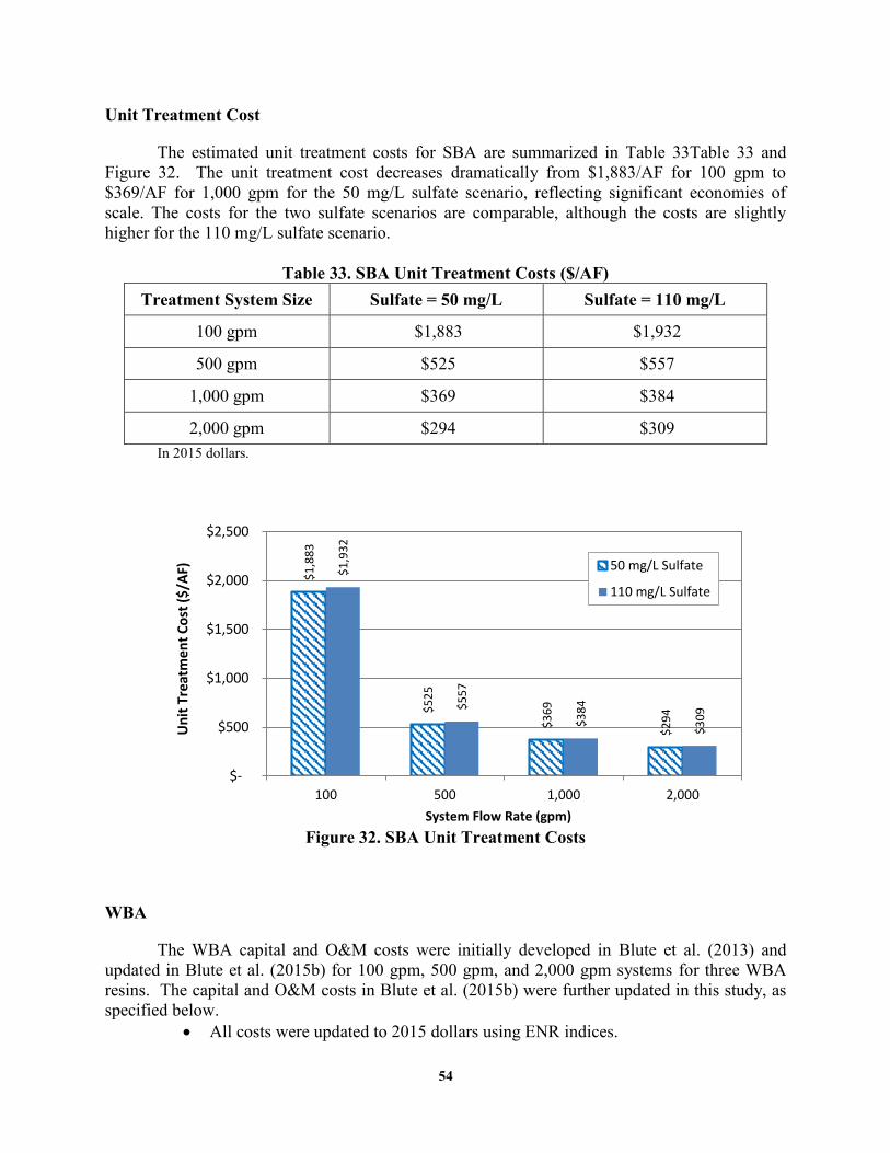
54

Unit Treatment Cost

The estimated unit treatment costs for SBA are summarized in Table 33Table 33 and Figure 32. The unit treatment cost decreases dramatically from $1,883/AF for 100 gpm to $369/AF for 1,000 gpm for the 50 mg/L sulfate scenario, reflecting significant economies of scale. The costs for the two sulfate scenarios are comparable, although the costs are slightly higher for the 110 mg/L sulfate scenario.

Table 33. SBA Unit Treatment Costs ($/AF)

Treatment System Size Sulfate = 50 mg/L Sulfate = 110 mg/L

100 gpm $1,883 $1,932

500 gpm $525 $557

1,000 gpm $369 $384

2,000 gpm $294 $309 In 2015 dollars.

Figure 32. SBA Unit Treatment Costs

WBA

The WBA capital and O&M costs were initially developed in Blute et al. (2013) and updated in Blute et al. (2015b) for 100 gpm, 500 gpm, and 2,000 gpm systems for three WBA resins. The capital and O&M costs in Blute et al. (2015b) were further updated in this study, as specified below.

All costs were updated to 2015 dollars using ENR indices.

$1

,88

3

$5

25

$3

69

$2

94

$1

,93

2

$5

57

$3

84

$3

09

$-

$500

$1,000

$1,500

$2,000

$2,500

100 500 1,000 2,000

Un

it T

reat

men

t C

ost

($

/AF)


50 mg/L Sulfate

110 mg/L Sulfate

55

The aeration system cost was updated from the previous cost for aluminum forced draft aerator to that for aeration towers (which are expected to be more efficient for carbon dioxide removal).

An antiscalant feed system was added to prevent calcium precipitation on the aeration system.

Capital and O&M costs for 1000 gpm were developed. Purolite S106 was used as the WBA resin for cost estimates in this study. The

Blute et al. (2015) cost estimates suggested comparable capital and O&M costs based on the three WBA resins (PWA7, S106 and SIR-700).

WBA resin life was assumed to be 383,000 BVs based on the recent demonstration test results at City of Glendale, California.

Staff time to operate and maintain a WBA system was updated to 0.4 FTE for systems equal to or below 1,000 gpm and 0.65 FTE for a 2,000-gpm system.

Analytical costs were updated based on an improved understanding of the WBA process monitoring requirements.

Figure 33 shows the WBA process flow diagram, for which capital and O&M costs were

developed/updated. The process includes pre- and post-pH adjustment systems (CO2 and aeration). Alternatively, acid and caustic soda can be used for pre- and post-pH adjustment. Aeration off-gas treatment was included at Glendale as its water contains VOCs which require off gas treatment using vapor phase GAC (VPGAC). However, for water sources without VOCs, aeration off-gas treatment is not needed. Thus, the capital and O&M costs in this study do not include aeration off-gas treatment.

Figure 33. WBA Process Flow Diagram

56

The WBA design criteria remained the same as in Blute et al. (2015b) as listed in Table 34.

Table 34. WBA Design Criteria WBA System Specifications 100 gpm 500 gpm 1,000 gpm 2,000 gpm

IX Vessel Configuration 1 lead/lag train

1 lead/lag train

1 lead/lag train

2 lead/lag trains

Total Number of Vessels 2 2 2 4

Vessel Diameter (ft) 4 8 12 12

Volume of Resin per Vessel (cf) 50 250 500 500

Total Resin Volume for First Fill (cf)

100 500 1,000 2,000

Surface loading rate (gpm/sf) 8.0 9.9 8.8 8.8

HLR (gpm/cf) 2.0 2.0 2.0 2.0

EBCT per Vessel (minute) 3.74 3.74 3.74 3.74

Operating pH 6.0 6.0 6.0 6.0

HLR – Hydraulic Loading Rate EBCT – Empty Bed Contact Time

Capital Cost


Excess capacity for redundancy was not included unless otherwise noted. A raw water pump was assumed to already exist with adequate pump pressure to

convey the water flow through the WBA process. Booster pumps were assumed to be required to lift the water through an aeration tower for post-pH adjustment.

Product water pumping and storage were not included. Land cost was not included. Equipment/operator building was not included. Pumps (i.e., chemical feed, waste discharge) included one standby unit to ensure

uninterrupted service in the case of equipment maintenance. Carbon dioxide feed systems were sized based on the design water quality and

RTW modeling of CO2 dose needed to achieve pH 6.0. First fill resin costs were included in capital cost. Purolite S106 was selected as

the WBA resin. Booster pumping to transfer the ion exchange effluent for post-pH adjustment was

assumed to provide 15-ft of additional pressure at each design flow rate. Aeration was designed for CO2 stripping to achieve a positive Langelier

Saturation Index (LSI) and Calcium Carbonate Precipitation Potential (CCPP).

57

Aeration tower was used (instead of aluminum forced draft aerators) as it was expected to provide more effective CO2 removal.

An antiscalant feed system was included to prevent calcium carbonate precipitation on aerators.

Aeration off-gas was not included in the capital costs. However, aeration off-gas treatment (e.g. VPGAC) would be needed for water sources with high VOCs levels.

WBA wastewater from resin change-out was assumed to be temporarily stored in a Baker tank and discharged to the sewer. No wastewater storage tank was included in capital cost.

Concrete equipment pads for the CO2 feed system, ion exchange system, and aeration tower were assumed to cost $1,330 per cubic yard, reflecting adjusted cost to 2015 dollars.

The estimated capital costs for WBA are summarized in Table 35.

Table 35. WBA Capital Costs Treatment System Size Purolite S106

100 gpm $1,433,000

500 gpm $2,887,000

1,000 gpm $3,645,000

2,000 gpm $6,172,000 Accuracy range is -30% to +50%. In 2015 dollars.

O&M Cost

O&M costs were developed for WBA systems and included estimated annual costs for electricity, chemicals, resin replacement, spent resin and backwash wastewater disposal, other consumables (e.g., bag filters), labor, maintenance and spare parts, and analytical costs.

O&M costs for each system size were developed based on the following assumptions:

A utilization rate of 100% of the design flow was assumed. No blending/ flow bypass was considered in the cost estimate. Electricity was assumed to cost $0.106 per kilowatt hour (kWh) in 2015 dollars. CO2 costs were based on the estimated dose required to achieve pH 6.0. Resin replacement costs were based on 383,000 bed volumes as observed at City

of Glendale. Unit resin cost was estimated as $305 per cubic feet, including tax, freight. A fixed installation cost of $10,000 was included for each resin replacement.

58

Spent resin was assumed to be non-RCRA hazardous waste and Technically Enhanced Naturally Occurring Radioactive Material (TENORM) with a disposal cost of $365/cf.

Baker tank rental cost was based on $2,247 for one 21,000-gallon tank, including tank delivery and pickup. For 100, 500 and 1000 gpm, one 21,000-gallon Baker tank is included. For 2,000 gpm, two 21,000-gallon Baker tanks are included.

Backwash wastewater disposal costs were based on discharge to the sewer without treatment at a cost of $3.15 per hundred cubic feet, plus a quarterly discharge fee of $945, which is adjusted based on the costs for WBA wastewater disposal incurred at Glendale, in 2015 dollars.

Labor costs were estimated based on $105,000 per FTE per year (loaded). Staff time to operate and maintain a WBA system was assumed to require 0.4 FTE for ≤ 1,000 gpm and 0.65 FTE for 2,000 gpm.

Bag filters were assumed to require replacement every quarter based on vendor quotes.

Maintenance costs were estimated to be 1% of total installed equipment costs. Analytical costs were developed based on a water quality monitoring schedule

updated from the Glendale Phase III Demonstration study and averages of quotes from two laboratories.

Annual O&M costs for WBA are summarized in Table 36.

Table 36. WBA Annual O&M Costs

Treatment System Size Purolite S106 100 gpm $113,000 500 gpm $221,000

1,000 gpm $356,000 2,000 gpm $655,000

In 2015 dollars.

The 20-year NPV of O&M costs for WBAs are summarized in Table 37.

Table 37. WBA 20-year NPV of O&M Costs Treatment System Size Purolite S106

100 gpm $1,900,000

500 gpm $3,700,000

1,000 gpm $6,000,000

2,000 gpm $11,000,000 20-year NPV O&M based on 2.5% inflation and a 4.5% discount rate in 2015 dollars.

59

Unit Treatment Cost

Unit treatment costs for WBA are presented in Table 38 and Figure 34.

Table 38. WBA Unit Treatment Costs ($/AF) Treatment System Size Purolite S106

100 gpm $1,384

500 gpm $549

1,000 gpm $394

2,000 gpm $350

Figure 34. WBA Unit Treatment Costs

UNIT COST COMPARISON FOR RCF, SBA AND WBA

A comparison of the unit treatment costs for all technologies are summarized below in Figure 35. Unit costs increase with reduced system flowrates into treatment facility.

$1

,38

4

$5

49

$3

94

$3

50

$300

$500

$700

$900

$1,100

$1,300

$1,500

100 500 1,000 2,000

Un

it T

reat

me

nt

Co

st (

$/A

F)


60

Figure 35. RCF, SBA and WBA Unit Treatment Costs

$2

,79

5

$9

25

$6

27

$5

09

$1

,93

9

$5

75

$3

86

$3

19

$1

,88

3

$5

25

$3

69

$2

94

$1

,93

2

$5

57

$3

84

$3

09

$1

,38

4

$5

49

$3

94

$3

50

$0

$400

$800

$1,200

$1,600

$2,000

$2,400

$2,800

$3,200

100 500 1,000 2,000

Un

it T

reat

me

nt

Co

st (

$/A

F)


RCF with Recycle

RCF without Recycle

SBA (50 mg/L of Sulfate)

SBA (110 mg/L of Sulfate)

WBA

61

CHAPTER 8. LAYOUTS AND DRAWINGS

Site layouts and preliminary design drawings were developed for RCF, SBA and WBA for a 1,000 gpm system to compare the required footprints. The Glendale’s RCF demonstration process site was used as the site for the layouts and drawings as an example.

RCF

A site plan, equipment layout, and a process flow diagram were developed for RCF without recycle and RCF with recycle. Figures 36, 37 and 38 show the site plan, equipment, and a process flow diagram layout for RCF without recycle, respectively. The estimated total equipment footprint is 1,455 sf. The minimum site footprint is 8,540 sf. Figures 39, 40 and 41 show the site plan, equipment and PFD layout for RCF with recycle. The estimated total equipment and site footprints are 3,385 sf and 13,060 sf, respectively. RCF with recycle would require much more space for equipment and a larger site than RCF without recycle.

SBA

A site plan, equipment layout, and a process flow diagram are shown for SBA in Figures 42, 43 and 44, respectively. The estimated total equipment and site footprints are 1,715 sf and 11,140 sf, respectively. The footprints are slightly larger but comparable to RCF without recycle.

WBA

A site plan, equipment layout, and a process flow diagram are shown for WBA in Figures 45, 46 and 47, respectively. The estimated total equipment and site footprints are 970 sf and 8,540 sf, respectively. The equipment footprint is significantly smaller than SBA or RCF without recycle. Thus, WBA may be preferred for treatment sites with a limited space.

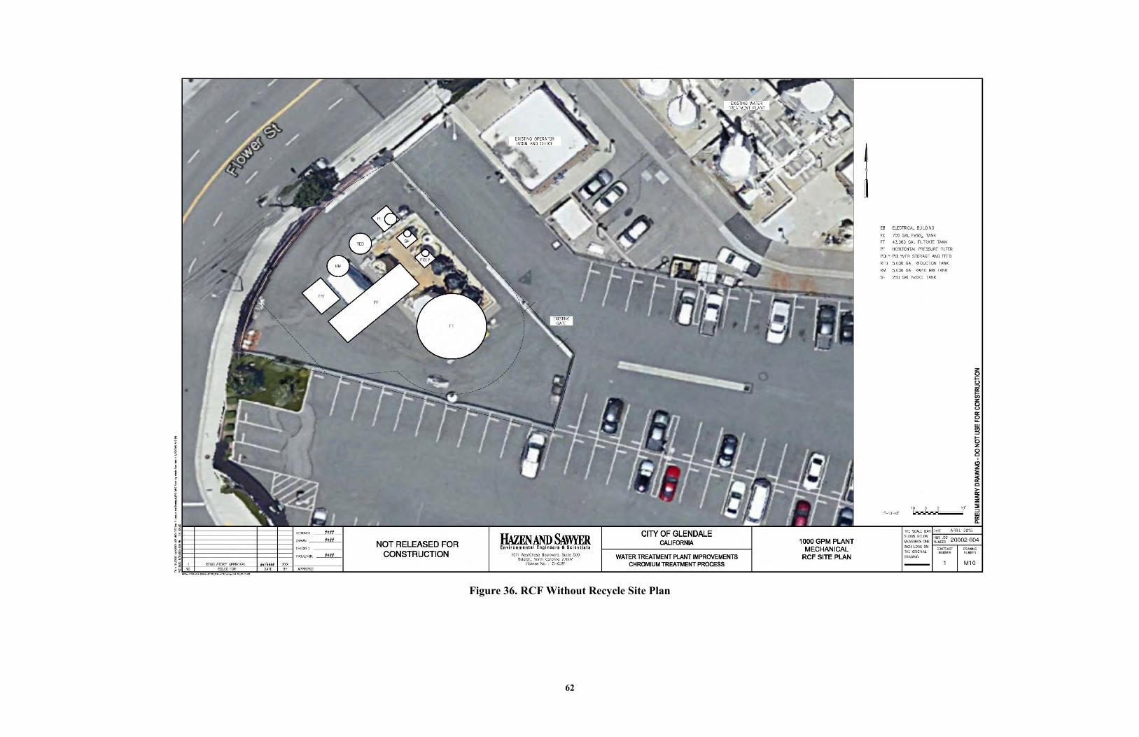
62

Figure 36. RCF Without Recycle Site Plan

63

Figure 37. RCF Without Recycle Equipment Layout

64

Figure 38. RCF Without Recycle PFD

65

Figure 39. RCF With Recycle Site Plan

66

Figure 40. RCF With Recycle Equipment Layout

67

Figure 41. RCF With Recycle PFD

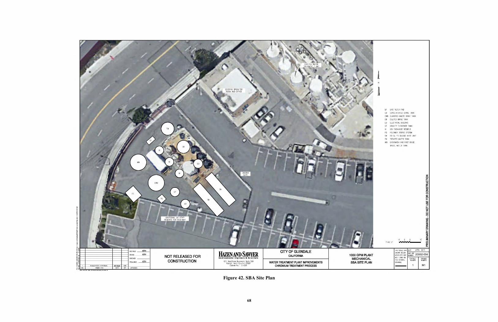
68

Figure 42. SBA Site Plan

69

Figure 43. SBA Equipment Layout

70

Figure 44. SBA PFD

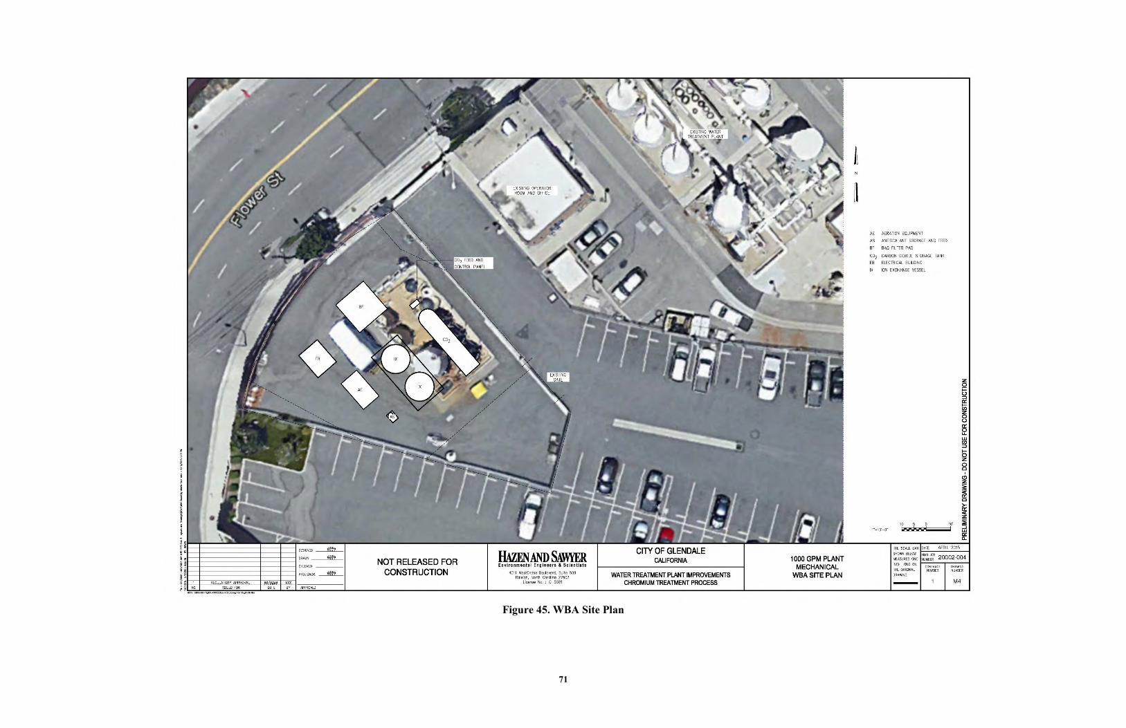
71

Figure 45. WBA Site Plan

72

Figure 46. WBA Equipment Layout

73

Figure 47. WBA PFD

74

CHAPTER 9. BLENDING ANALYSIS

Cr(VI) MCL compliance can be achieved by a non-treatment or treatment approach. Non-treatment includes using an alternative source or blending the affected source with another source containing lower Cr(VI) concentrations. When treatment is needed, the Cr(VI) treatment process can be designed to treat the whole flow or only a portion of the flow, with blending of treated water and bypassed water to achieve the Cr(VI) treatment goal. The advantage of the blending approach is that the treatment system size is smaller, thus requiring less capital cost. However, the Cr(VI) treatment goal may be lower for the portion treated to allow blending with the bypass and ensure MCL compliance. As a result, the O&M cost is expected to be higher. For example, WBA and SBA resins are expected to need more frequent resin replacements. However, it was not obvious at the outset if the blending approach would be more cost effective than treating the whole flow. This chapter evaluates the cost benefits of using blending to allow treating a lower flow rate to comply with the MCL.

METHODOLOGY

Three scenarios were developed for this analysis (Table 39). First, a baseline scenario evaluated the treatment costs for RCF, WBA, and SBA with blending compared to without blending to achieve a treated Cr(VI) concentration of 8 µg/L. The second scenario evaluated the impact of key water quality parameters on treatment costs with blending compared to without blending. For WBA, the key water quality parameter affecting treatment costs is alkalinity. Two alkalinity levels of 250 and 100 mg/L as CaCO3 were evaluated in this scenario. For SBA, the key water quality parameter affecting treatment costs is sulfate. Two sulfate concentrations (20 and 50 mg/L), in addition to the Glendale sulfate level of 110 mg/L in the baseline scenario, were evaluated in this analysis. RCF treatment costs are not significantly affected by water qualities, and thus were not evaluated further. The third scenario assessed the impacts of Cr(VI) treatment goal on treatment costs with blending compared to without blending. The Cr(VI) treatment goal affects the resin life for WBA and SBA both with and without blending, and also affects the water quantities to be treated with blending for RCF, WBA and SBA. Three treatment goals were evaluated, i.e. 8, 6 and 4 µg/L.

Table 39. Overview of Scenarios

No. Scenario Purpose

1 Baseline Evaluates the treatment costs of blending versus non-blending for RCF, WBA, and SBA using Glendale’s water quality.

2 Effects of Water Quality Evaluates the impacts of key water quality on the comparison of blending versus non-blending for WBA and SBA.

3 Effects of Treatment Goal Evaluates the impacts of Cr(VI) treatment goal on the comparison of blending versus non-blending for RCF, WBA and SBA.

75

Capital costs were estimated using cost curves as shown in Figures 48 and 49, which

were developed based on the capital costs described in Chapter 7. O&M costs were estimated using the same methodology described in Chapter 7. Unit treatment costs were used to compare the costs for blending versus non-blending, which incorporated both capital and O&M costs. Unit treatment costs were calculated based on a 20-year life cycle and a 5% interest rate.

Figure 48. Capital Cost Curves for RCF with and without Recycle

Figure 49. Capital Cost Curves for WBA and SBA

y = 2046x + 2E+06R² = 0.9979

y = 2362.9x + 2E+06R² = 0.9791

$0

$1,000,000

$2,000,000

$3,000,000

$4,000,000

$5,000,000

$6,000,000

$7,000,000

$8,000,000

0 500 1000 1500 2000 2500

Cap

ital

($

)

Treatment Flow Rate (gpm)

RCF without Recycle

RCF with Recycle

y = 2915.4x + 1E+06R² = 0.9993

y = 2402.2x + 1E+06R² = 0.9875

$0

$1,000,000

$2,000,000

$3,000,000

$4,000,000

$5,000,000

$6,000,000

$7,000,000

$8,000,000

0 500 1000 1500 2000 2500

Cap

ital

($

)

Treatment Flow Rate (gpm)

SBA

WBA

76

For all scenarios, a system flow rate of 1,000 gpm was used, which represents a typical groundwater well size in California. For a non-blending approach, the treatment flow rate is 1,000 gpm. For a blending approach, the treatment flow rate was calculated based on the Cr(VI) concentrations in raw water, the Cr(VI) treatment target after blending and the assumed Cr(VI) concentration in the treated water using mass balance as illustrated in Figure 50. Based on pilot and demonstration testing, it was assumed that WBA and SBA can effectively remove Cr(VI) to below 2 µg/L, while RCF can effectively remove Cr(VI) to below 5 µg/L.

Figure 50. Approach Used to Estimate Treatment Flow Rate

SCENARIO 1. BASELINE

Table 40 summarizes the design water quality on which the treatment costs were estimated for blending versus non-blending in Scenario 1. Raw water Cr(VI) concentration was selected as 15 µg/L to represent typical Cr(VI) concentrations in affected groundwater sources in California. Other water quality parameters were based on one of Glendale’s wells GN-3. This water contained a relatively high level of alkalinity, which requires a high carbon dioxide dose for pH adjustment for WBA. It also contains a relatively high level of sulfate, which is expected to result in more frequent resin regenerations for SBA.

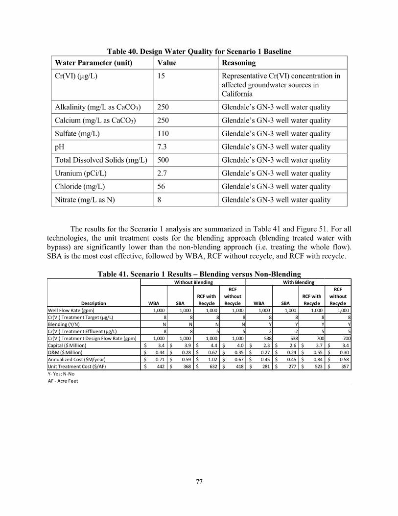
77

Table 40. Design Water Quality for Scenario 1 Baseline Water Parameter (unit) Value Reasoning

Cr(VI) (µg/L) 15 Representative Cr(VI) concentration in affected groundwater sources in California

Alkalinity (mg/L as CaCO3) 250 Glendale’s GN-3 well water quality

Calcium (mg/L as CaCO3) 250 Glendale’s GN-3 well water quality

Sulfate (mg/L) 110 Glendale’s GN-3 well water quality

pH 7.3 Glendale’s GN-3 well water quality

Total Dissolved Solids (mg/L) 500 Glendale’s GN-3 well water quality

Uranium (pCi/L) 2.7 Glendale’s GN-3 well water quality

Chloride (mg/L) 56 Glendale’s GN-3 well water quality

Nitrate (mg/L as N) 8 Glendale’s GN-3 well water quality

The results for the Scenario 1 analysis are summarized in Table 41 and Figure 51. For all

technologies, the unit treatment costs for the blending approach (blending treated water with bypass) are significantly lower than the non-blending approach (i.e. treating the whole flow). SBA is the most cost effective, followed by WBA, RCF without recycle, and RCF with recycle.

Table 41. Scenario 1 Results – Blending versus Non-Blending

WBA SBA

RCF with

Recycle

RCF

without

Recycle WBA SBA

RCF with

Recycle

RCF

without

Recycle

Well Flow Rate (gpm) 1,000 1,000 1,000 1,000 1,000 1,000 1,000 1,000

Cr(VI) Treatment Target (µg/L) 8 8 8 8 8 8 8 8

Blending (Y/N) N N N N Y Y Y Y

Cr(VI) Treatment Effluent (µg/L) 8 8 5 5 2 2 5 5

Cr(VI) Treatment Design Flow Rate (gpm) 1,000 1,000 1,000 1,000 538 538 700 700

Capital ($ Million) 3.4$ 3.9$ 4.4$ 4.0$ 2.3$ 2.6$ 3.7$ 3.4$

O&M ($ Million) 0.44$ 0.28$ 0.67$ 0.35$ 0.27$ 0.24$ 0.55$ 0.30$

Annualized Cost ($M/year) 0.71$ 0.59$ 1.02$ 0.67$ 0.45$ 0.45$ 0.84$ 0.58$

Unit Treatment Cost ($/AF) 442$ 368$ 632$ 418$ 281$ 277$ 523$ 357$

Y- Yes; N-No

AF - Acre Feet

Without Blending With Blending

Description

78

Figure 51. Treatment Costs for Blending vs. Non-Blending in Scenario 1

SCENARIO 2. EFFECTS OF WATER QUALITY

Scenario 2 evaluates the effects of water quality on the comparison of blending versus non-blending for WBA and SBA. For WBA, alkalinity was selected as the key water quality that impacts treatment cost by affecting carbon dioxide dose. Two alkalinity concentrations were selected, 250 mg/L mg/L as CaCO3 and 100 mg/L as CaCO3, representing relatively high and moderate alkalinity concentrations. Other water quality parameters may also affect WBA cost. For example, Cr(VI) and sulfate concentrations in raw water may affect WBA resin life. However, the magnitude of the impacts has not quantified. Thus, these parameters were not evaluated in this study. For SBA, sulfate is considered the key water quality that drives the resin regeneration frequency. With a higher sulfate concentration, SBA regeneration frequency significantly increases. Including the sulfate level in Scenario 1, a total of three sulfate concentrations were evaluated in this scenario - 20 mg/L, 50 mg/L and 110 mg/L.

The results for WBA with the two alkalinity levels are summarized in Table 42 and

Figure 52. For both alkalinity levels, the blending approach generates significantly lower unit treatment costs by $136 to $161/AF. The treatment cost for the lower alkalinity concentration was estimated to be significantly lower than the higher concentration.

$442

$368

$632

$418

$281 $277

$523

$357

$0

$100

$200

$300

$400

$500

$600

$700

WBA SBA RCF with Recycle RCF without Recycle

Un

it T

reat

me

nt

Co

st (

$/A

F)Without Blending With Blending

79

Table 42. Blending versus Non-Blending for WBA with Different Alkalinity Concentrations

Figure 52. Effect of Alkalinity on WBA Treatment Costs for Blending vs. Non-Blending

Effects of sulfate levels on SBA treatment costs for blending and non-blending are summarized in Table 43 and Figure 53. For all three sulfate levels, the blending approach was estimated to have lower unit treatment costs than the non-blending approach. The cost savings were estimated in the range of $87/AF to $286/AF. The unit treatment costs also decrease significantly with sulfate level, as less resin regenerations were expected for a lower sulfate concentration.

Alkalinity = 250

mg/L as CaCO3

Alkalinity = 100

mg/L as CaCO3

Alkalinity = 250

mg/L as CaCO3

Alkalinity = 100

mg/L as CaCO3

Well Flow Rate (gpm) 1,000 1,000 1,000 1,000

Cr(VI) Treatment Target (µg/L) 8 8 8 8

Blending (Y/N) N N Y Y

Cr(VI) Treatment Effluent (µg/L) 8 8 2 2

Cr(VI) Treatment Design Flow Rate (gpm) 1,000 1,000 538 538

Capital ($ Million) 3.4$ 3.4$ 2.3$ 2.3$

O&M ($ Million) 0.44$ 0.35$ 0.27$ 0.22$

Annualized Cost ($M/year) 0.71$ 0.62$ 0.45$ 0.40$

Unit Treatment Cost ($/AF) 442$ 386$ 281$ 250$

Y- Yes; N-No

AF - Acre Feet

WBA

Description

$442

$386

$281 $250

$0

$100

$200

$300

$400

$500

$600

$700

Alkalinity = 250 mg/L as CaCO3 Alkalinity = 100 mg/L as CaCO3

Un

it T

reat

me

nt

Co

st (

$/A

F)


80

Table 43. Blending versus Non-Blending for SBA with Different Sulfate Concentrations

Figure 53. Effect of Sulfate on SBA Treatment Costs for Blending vs. Non-Blending

SCENARIO 3. EFFECTS OF TREATMENT GOAL

Scenario 3 evaluates the effects of the Cr(VI) treatment goal on the comparison of non-blending versus blending. Three treatment goals were evaluated, including 4, 6 and 8 µg/L. The design water quality were assumed to be the same as in Scenario 1. The estimated resin bed volumes for WBA for the different treatment goals are summarized in Table 44, which were selected based on the demonstration-scale testing at Glendale using PWA7 resin. The resin bed volumes for SBA were estimated using the formulas shown in Figure 54, which were developed

Sulfate = 110

mg/L

Sulfate = 50

mg/L

Sulfate = 20

mg/L

Sulfate = 110

mg/L

Sulfate = 50

mg/L

Sulfate = 20

mg/L

Well Flow Rate (gpm) 1000 1,000 1,000 1,000 1,000 1,000

Cr(VI) Treatment Target (µg/L) 8 8 8 8 8 8

Blending (Y/N) N N N Y Y Y

Cr(VI) Treatment Effluent (µg/L) 8 8 8 2 2 2

Cr(VI) Treatment Design Flow Rate (gpm) 1000 1,000 1,000 538 538 538

Capital ($ Million) 3.9$ 3.9$ 3.9$ 2.6$ 2.6$ 2.6$

O&M ($ Million) 0.59$ 0.25$ 0.24$ 0.24$ 0.22$ 0.21$

Annualized Cost ($M/year) 0.91$ 0.56$ 0.56$ 0.45$ 0.42$ 0.42$

Unit Treatment Cost ($/AF) 563$ 350$ 345$ 277$ 262$ 258$

Y- Yes; N-No

AF - Acre Feet

SBA

Description

$563

$350 $345

$277 $262 $258

$0

$100

$200

$300

$400

$500

$600

$700

Sulfate = 110 mg/L Sulfate = 50 mg/L Sulfate = 20 mg/L

Un

it T

reat

me

nt

Co

st (

$/A

F)


81

based on several SBA studies (Blute et al., 2015b; Chowdhury et al., 2015; Najm et al., 2015; Seidel et al., 2014).

Table 44. Assumed WBA Resin Bed Volumes for Different Cr(VI) Treatment Goals

Cr(VI) Treatment Goal Lead Bed Resin Bed Volumes for WBA

4 µg/L 357,000

6 µg/L 370,000

8 µg/L 383,000

Figure 54. SBA Bed Volumes as a Function of Sulfate Concentration for Cr(VI)

Breakthrough Greater than 4, 6, and 8 µg/L The results for WBA are summarized in Table 45 and Figure 55. For all treatment goals,

the unit treatment costs for the blending approach were estimated significantly lower than the non-blending approach. The cost savings decrease with a lower Cr(VI) treatment goal. The highest cost saving is $161/AF for the 8 µg/L treatment goal; while the smallest cost saving is $55/AF for the 4 µg/L treatment goal. This accounts for an overall costs savings between 12 to 36% as shown in Figure 55 from extensive to minimal treatment to ensure Cr(VI) compliance when comparing the blending to non-blending approach.

y = 258416x-0.833

R² = 0.8036

y = 265218x-0.887

R² = 0.8366y = 226428x-0.903

R² = 0.87590

5,000

10,000

15,000

20,000

25,000

30,000

- 50 100 150 200 250

Re

sin

Lif

e a

s B

ed

Vo

lum

es

Sulfate (mg/L)

Breakthrough to greater than 8 ug/L



82

Table 45. Blending versus Non-Blending for WBA with Different Treatment Goals

Figure 55. Effect of Treatment Goal on WBA Treatment Costs for Blending vs. Non-

Blending

The results for SBA are summarized in Table 46 and Figure 56. The blending approach

for the SBA process exhibited similar trends as the WBA process, contributing to an overall costs savings compared to the non-blending approach. The highest costs savings is $91/AF for the 8 µg/L treatment goal, while the smallest costs savings is $29/AF when extensive treatment is carried out to meet the 4 µg/L goal, resulting in an overall costs savings between 7 to 25%.

Well Flow Rate (gpm) 1,000 1,000 1,000 1,000 1,000 1,000




Cr(VI) Treatment Design Flow Rate (gpm) 1,000 1,000 1,000 538 692 846

Capital ($ Million) 3.4$ 3.4$ 3.4$ 2.3$ 2.7$ 3.0$

O&M ($ Million) 0.44$ 0.44$ 0.45$ 0.27$ 0.32$ 0.39$



Y- Yes; N-No

AF - Acre Feet

Description Without Blending With Blending

WBA WBA

$442 $442 $448

$281

$331

$393

$0

$100

$200

$300

$400

$500

$600

$700

Treatment Goal = 8 µg/L Treatment Goal = 6 µg/L Treatment Goal = 4 µg/L

Un

it T

reat

me

nt

Co

st (

$/A

F)


83

Table 46. Blending versus Non-Blending for SBA with Different Treatment Goals

Figure 56. Effect of Treatment Goal on SBA Treatment Costs for Blending vs. Non-

Blending

The results for the RCF process, without and with recycle, are summarized in Table 47 along with supporting site plan layouts depicted in Figures 36 and 39, respectively. The treatment goal of 4 µg/L is ruled out due to RCF process limitations to effectively reduce the Cr(VI) levels down to around 5 µg/L, thus the Cr(VI) treatment goals evaluated only consider 6 µg/L and 8 µg/L. The blending approach continues to sustain an advantage over the non-blending approach for the RCF process in terms of cost savings, regardless of whether the clarified backwash waste stream is recycled or not. However, the unit treatment costs suggests that operating the RCF process with recycle results in greater savings yielding $109/AF for the 8

Well Flow Rate (gpm) 1,000 1,000 1,000 1,000 1,000 1,000




Cr(VI) Treatment Design Flow Rate (gpm) 1,000 1,000 1,000 538 692 846

Capital ($ Million) 3.9$ 3.92$ 3.92$ 2.6$ 3.0$ 3.5$

O&M ($ Million) 0.28$ 0.29$ 0.31$ 0.24$ 0.26$ 0.30$



Y- Yes; N-No

AF - Acre Feet

Without Blending

SBA

With Blending

SBA

Description

$368 $375 $387

$277 $311

$358

$0

$100

$200

$300

$400

$500

$600

$700

Treatment Goal = 8 µg/L Treatment Goal = 6 µg/L Treatment Goal = 4 µg/L

Un

it T

reat

me

nt

Co

st (

$/A

F)


84

µg/L treatment goal and $34/AF for the 6 µg/L treatment goal compared to the RCF process without recycling, achieving a slightly lower cost savings of $61/AF and $16/AF, respectively. Although the RCF without recycle option yields a lower unit treatment cost, the waste volume generated may be significantly larger and will have an adverse contribution on the net overall costs. The range of cost savings when comparing the treatment goals are similar for both conditions as shown in Figure 57, yielding a range from 5 to 17% with recycle and 4 to 15% without recycle.

Table 47. Blending versus Non-Blending for RCF with Different Treatment Goals

Figure 57. Effect of Treatment Goal on RCF Treatment Costs for Blending vs. Non-

Blending

Well Flow Rate (gpm) 1,000 1,000 1,000 1,000 1,000 1,000 1,000 1,000

Cr(VI) Treatment Target (µg/L) 8 6 8 6 8 6 8 6

Blending (Y/N) N N Y Y N N Y Y

Cr(VI) Treatment Effluent (µg/L) 5 5 5 5 5 5 5 5

Cr(VI) Treatment Design Flow Rate (gpm) 1000 1000 700 900 1000 1000 700 900

Capital ($ Million) 4.4$ 4.4$ 3.7$ 4.1$ 4.0$ 4.0$ 3.4$ 3.8$

O&M ($ Million) 0.67$ 0.67$ 0.55$ 0.63$ 0.35$ 0.35$ 0.30$ 0.34$

Annualized Cost ($M/year) 1.02$ 1.02$ 0.84$ 0.97$ 0.67$ 0.67$ 0.58$ 0.65$

Unit Treatment Cost ($/AF) 632$ 632$ 523$ 598$ 418$ 418$ 357$ 402$

Y- Yes; N-No

AF - Acre Feet

RCF without Recycle

With BlendingWithout Blending

RCF with Recycle RCF without RecycleRCF with Recycle

Description With Blending Without Blending

$632 $632

$418 $418

$523

$598

$357

$402

$0

$100

$200

$300

$400

$500

$600

$700

Treatment Goal = 8 µg/LTreatment Goal = 6 µg/LTreatment Goal = 8 µg/LTreatment Goal = 6 µg/L

Un

it T

reat

me

nt

Co

st (

$/A

F)


RCF with Recycle RCF without Recycle

85

86


Cr(VI) MCL compliance can be achieved with two approaches, including treatment and non-treatment approaches. Treatment can be combined with non-treatment of a portion of the flow (i.e., blending) to achieve an overall concentration below the MCL. Advantages to the blending approach include smaller treatment footprint and lower capital cost, but it requires more robust treatment to ensure that the treated stream sustains a low enough concentration to be used to dilute the bypass stream. The costs and benefits of integrating blending to afford a lower treatment flow rate was evaluated for three scenarios comparing the established Cr(VI) treatment technologies of SBA, WBA, and RCF.

Scenario 1 served as the baseline scenario to evaluate the treatment costs of blending

versus full flow treatment for RCF, WBA, and SBA using Glendale’s water quality to achieve a treatment target of 8 µg/L. The blending option was found to offer significant savings in terms of unit treatment costs compared to the non-blending option for all technologies.

Scenario 2 evaluated the impacts of key water quality on the comparison of blending

versus non-blending for WBA and SBA. Alkalinity served as the key limiting factor for the WBA process. Sulfate was considered the key water quality impacting the SBA process. Despite the range of alkalinity and sulfate concentrations used in this analysis, the blending option was found to offer an advantage over the non-blending option. The unit treatment costs for each process decrease with lower alkalinity and sulfate levels overall.

Scenario 3 evaluated the impact of Cr(VI) treatment goals on the comparison of blending

versus non-blending for RCF, WBA, and SBA. Cr(VI) treatment targets evaluated included 4, 6, and 8 µg/L for WBA and SBA, and 6 and 8 µg/L for RCF. The blending option continued to offer an overall cost savings over the non-blending option for the different treatment targets

87

CHAPTER 10. SUMMARY AND CONCLUSIONS

Prior demonstration-scale testing had provided indications that the RCF process could be improved to decrease footprint and cost. This study resolved a number of outstanding questions to yield an optimized approach for RCF.

RCF operational conditions were optimized to include 2 mg/L iron dose, 5 minutes of

reduction time, inline chlorine injection and centrifugal filtration pumping, which resulted in significant cost savings and reduced the system footprint. If a higher Cr(VI) concentration is present, a higher iron dose (e.g., 3 mg/L for addressing 100 µg/L Cr(VI)) will be more effective than 2 mg/L. Optimization of the chlorine dosing process was able to alleviate the concern for re-oxidation of Cr(III) to Cr(VI) while sustaining effective ferrous oxidation for effective removal via the filtration process.

A progressive cavity pump was initially selected for the study with intention to preserve

the flocculated particles inhibited by the polymer to ensure effective filtration of the chromium and iron in the source water. A centrifugal pump was tested in this study as a cost-effective alternative to be integrated into the RCF process to replace the existing pump for additional cost savings. The RCF facility operated with the centrifugal pump under the recommended ferrous dose (2 and 3 mg/L) and reduction times (5 and 10 minutes) previously determined for effective Cr(VI) reduction. The test runs yielded results similar compared to that of the progressive cavity pump and confirmed that a centrifugal pump can be used for cost savings.

Updated cost analysis of RCF, WBA, and SBA was performed with each being optimized

to yield lower estimates. Optimization of the RCF process from bench and demonstration-scale testing resulted in an overall cost savings. Compared to the cost analysis previously completed by Blute et al. (2015b), the capital cost savings range from $0.1 to $0.6 million for different systems as a result of optimized RCF conditions (centrifugal pump, lower reduction time and ferrous dose, inline chlorine injection), reducing equipment cost and system footprint. The O&M cost savings range from $0.1 to $0.5 million (depending on whether recycle is considered) are impacted by the reduced chemical doses and labor.

Overall, SBA was found to have the lowest treatment cost for 500 gpm and above, while

WBA has the lowest cost for 100 gpm. RCF with recycle generally requires a higher cost due to the additional infrastructure and operations necessary for recycling wastewater. However, the cost differences between SBA, WBA, and RCF without recycle are not large. Other factors, such as site space, sewer access and operational preference, must also be considered in process selection.

To determine the space requirements for each treatment process, site layout and

preliminary design drawings were developed for a 1,000 gpm system to compare the required footprint and space savings. WBA may be preferred for treatment sites with limited space available, followed by RCF without recycle and SBA. The RCF process with recycle increase footprint requirement by 35% compared to non-recycle and requires the largest footprint of the

88

other processes. Alternately, SBA without brine treatment (which was not evaluated) could offer a smaller footprint than with brine treatment.

Blending analysis based on treatment of a 1,000 gpm well indicated that blending (i.e.,

treating a portion of the flow and then blending the treated water with untreated bypassed water) is more cost effective than treating the entire flow through the RCF, WBA or SBA, for a range of water quality and Cr(VI) treatment goals.

Overall, the results of this study were of great value in optimizing the treatment processes

and allowing a closer comparison of the best available technologies for Cr(VI) removal from drinking water. The extensive analysis completed over the years at Glendale, and optimized in this study, provides water agencies with testing of options and a basis for cost estimation of solutions.

89

CHAPTER 11. REFERENCES

Blute, N., Wu, X., Porter, K., Imamura, G., and McGuire, M., 2013. Hexavalent Chromium

Removal Research Project Report. California Department of Public Health, Sacramento, Calif. www.glendalewaterandpower.com/pdf/Chromium6Report2013.pdf. Blute, N.K., Wu, X., Cron, C., Porter, K., Fong, L., Froelich, D., Abueg, R. 2015a. Microfiltration in the RCF Process for Hexavalent Chromium Removal from Drinking Water. Water Research Foundation Report #4365. Denver, CO. Blute, N.K., Wu, X., Imamura, G., Song, Y., Porter, K., Cron, C., Fong, L., Froelich, D., Abueg, R., Henrie, T., Ramesh, S., and Vallejo, F. 2015b. Assessment of Ion Exchange, Adsorptive

Media, and RCF for Cr(VI) Removal. Water Research Foundation Report #4423. Denver, CO. Chowdhury, Z., Bigley, S., Gonzalez, W., Porter, K.L., Francis, C., Imamura, G., Blute, N., Rhoades, J., Westerhoff, P., Bowen, A. 2015. Evaluation of Technologies for Hexavalent

Chromium Removal and Development of a Compliance Planning Approach. Water Research Foundation Report #4445 and 4516. Denver, CO. Coachella Valley Water District, 2015. Unpublished pilot testing of SBA resins. Najm, I., Brown, N.P., Seo, E., Gallagher, B., Gramith, K., Blute, N., Wu, X., Yoo, M., Liang, S., Maceiko, S., Kader, S., Lowery, J. 2014. Impact of Water Quality on Hexavalent Chromium

Removal Efficiency and Cost. Water Research Foundation Report #4450. Denver, CO. Seidel, C, Gorman, C., Ghosh, A., Dufour, T., Mead, C., Henderson, J., Li, X., Darby, J., Green, P., McNeill, L., Clifford, D., 2014. Hexavalent Chromium Treatment with Strong Base Anion

Exchange. Water Research Foundation Report #4488. Denver, CO.

Documents

Enhanced Reduction/Coagulation/ Filtration …mwdh2o.com/FAF PDFs/1a_GW_Glendale MWD Final Report.pdfEnhanced Reduction/Coagulation/ Filtration Testing for Removing Hexavalent Chromium