Embed Size (px)
Citation preview
Enhanced error estimator based on a nearlyequilibrated moving least squares recovery
technique for FEM and XFEM
J. J. Rodenas1 O. A. Gonzalez-Estrada2∗ F. J. Fuenmayor1
F. Chinesta3
August 29, 2018
1Centro de Investigacion de Tecnologıa de Vehıculos(CITV),Universitat Politecnica de Valencia, E-46022-Valencia, Spain.
2 Institute of Mechanics & Advanced Materials, Cardiff University, School ofEngineering, Queen’s Building, The Parade, Cardiff CF24 3AA Wales, UK.
3 EADS Corporate International Chair. Ecole Centrale de Nantes, Nantes, France.
Abstract
In this paper a new technique aimed to obtain accurate estimates of theerror in energy norm using a moving least squares (MLS) recovery-based pro-cedure is presented. We explore the capabilities of a recovery technique basedon an enhanced MLS fitting, which directly provides continuous interpolatedfields, to obtain estimates of the error in energy norm as an alternative tothe superconvergent patch recovery (SPR). Boundary equilibrium is enforcedusing a nearest point approach that modifies the MLS functional. Lagrangemultipliers are used to impose a nearly exact satisfaction of the internal equi-librium equation. The numerical results show the high accuracy of the pro-posed error estimator.
KEYWORDS: error estimation; equilibrated stresses; stress recovery; extended finite ele-
ment method; moving least squares
1 Introduction
During the last few decades numerical techniques, such as the finite element method(FEM), have been used to approximate the solution of real problems. In order toassess the quality of these approximations it is necessary to evaluate the error ob-tained in the simulation. Current methods used to estimate the discretization errorof finite element (FE) solutions are usually classified into different families: residualbased, recovery based, dual analysis techniques,... [1, 2, 3]. The use of recovery
∗Email: [email protected]
1
arX
iv:1
208.
6381
v1 [
mat
h.N
A]
31
Aug
201
2

based estimators is widespread due to their robustness and simple implementationinto existing FE codes.
Today, novel techniques such as the extended finite element method (XFEM) arebeing used to introduce a priori known information about the problem solution intothe FE formulation. The XFEM [4] enriches the classical FEM basis functions usinga partition of unity approach in order to capture the local features of the solutionin a cracked domain, i.e. the discontinuity of the displacement field along the crackfaces and the singularity of the stresses in the vicinity of the crack tip.
Although the XFEM provides highly accurate solutions, and significantly im-proves the modelling of certain types of problems, there is an urge to develop errorcontrol techniques for these kind of methods, mostly because of their increasingimportance and the fact that they use rather coarse discretizations. For example,recovery based error estimators for partition of unity methods have been developedin [5, 6, 7, 8], using the residual approach in [9, 10] and the constitutive relationerror (CRE) in [11]. In [12] the CRE is used for goal oriented error estimation inXFEM.
The enforcement of the internal and the boundary equilibrium equations forstress recovery has been previously considered in the literature as a mean to im-prove the quality of the recovered field. For patch based formulations, [13, 14]introduced the squares of the residuals of the equilibrium equations to the leastsquares functional solved in the recovery process through a penalty parameter. In[15] a point-wise enforcement of the internal equilibrium in the polynomial basis,used to represent the recovered stress at the support of each node, was presented.Then, boundary equilibrium conditions were applied on a set of sampling pointsin the part of the patch boundary that coincides with the domain boundary. TheSPR-C technique proposed in [16] imposed equilibrium constraints to the polyno-mial basis via Lagrange multipliers. The internal equilibrium was exactly satisfiedat each patch, and a Taylor expansion of the applied stresses was enforced alongthe Neumann contour. Then, a conjoint polynomial procedure [14] was used to ob-tain a continuous stress field. Later, in [7] this technique was extended to XFEMapproximations.
Procedures to smooth or to recover the stress field based on MLS have also beenused. In [17] a continuous stress field was obtained through local interpolation of thenodal displacement values using MLS. In [5] this same formulation was extended toXFEM problems, considering an enriched MLS basis and a diffraction criterion, andan error estimate for enriched approximations was proposed. In [18] a procedureto smooth the stresses for the meshless element free Galerkin (EFG) method usingMLS shape functions was described. In [19] a so called Statically Admissible StressRecovery Technique (SAR) that used MLS to fit the stress at sampling points waspresented. The SAR technique comprised basis functions which consider the in-ternal equilibrium equations and the local tractions conditions along the Neumannboundary. In [20] an extension of the SAR technique for XFEM was presented.Following the definition of pseudo-divergence-free field used in [21], we can say thatin references [19] and [20] the authors considered a pseudo-satisfaction of the in-ternal equilibrium equation. They indicated that accurate stresses were obtainedwith SAR, but they did not go further to evaluate any error estimate. In [22] dual
2

techniques were used in meshless methods to obtain an equilibrated dual problemusing MLS shape functions that approximate Airy stress functions.
The objective of this paper is to present an enhanced version of the MLS recoverytechnique to evaluate accurate estimates of the discretization error for FEM andXFEM problems that is based in the ideas presented in [7, 8, 16, 23]. The rationalebehind the proposed technique is to try to enforce the recovered stress field tosatisfy continuity (this property is directly provided following the MLS approach)and the equilibrium equations that are satisfied by the exact solution such thatrecovered stresses get closer to the exact stress field. An appropriate applicationof the equilibrium constraints is required to avoid discontinuities in the recoveredfield. For that reason, a novel approach to introduce the internal and boundaryequilibrium constraints is proposed. The procedure has been implemented in a FEcode where mesh refinement is based on element splitting and the use of constrainequations (Multi Point Constraints, MPC) to force C0 continuity at hanging nodes.SPR requires special treatment of these nodes because it is based on the meshtopology. The use of the proposed technique is more flexible as it is not constrainedby the topology of the finite element mesh. This feature is very powerful and itallows the direct use of the technique with isogeometric analysis with h-adaptiverefinement based on T-splines and in cases where the FE mesh is missing, like withmeshless methods or elements with an arbitrary number of sides.
Reference [23] showed that upper bounds of the error in energy norm can beobtained with recovery-based error estimators if the recovered stress field is staticallyadmissible. The recovered stresses resulting from the use of the technique proposedin this paper are continuous, satisfy the contour equilibrium equation and providea nearly exact satisfaction of the internal equilibrium equation (more accurate thanthe pseudo-satisfaction of the equilibrium equation used in previous works [19, 20]).Although the upper bound property is not guaranteed, the numerical results showthat the proposed technique yields sharp error estimates which nearly bound theexact error.
The paper is organised as follows: in Section 2 we present the reference prob-lems and their approximate solutions using FEM and XFEM. Section 3 deals withthe main aspects of error estimation in FE approximations and the moving leastsquares formulation considering equilibrium conditions. Finally, numerical resultsare presented in Section 4, and conclusions are drawn in Section 5.
2 Problem Statement and Solution
2.1 Problem statement
Let us consider the 2D linear elasticity problem. The unknown displacement fieldu, taking values in Ω ⊂ R2, is the solution of the boundary value problem given by
−∇ · σ (u) = b in Ω (1)
σ (u) · n = t on ΓN (2)
u = 0 on ΓD (3)
3
where ΓN and ΓD denote the Neumann and Dirichlet boundaries with ∂Ω = ΓN∪ΓDand ΓN ∩ ΓD = ∅. The Dirichlet boundary condition in (3) is taken homogeneousfor the sake of simplicity.
The weak form of the problem reads: Find u ∈ V such that
∀v ∈ V a(u,v) = l(v), (4)
where V is the standard test space for the elasticity problem such that V = v | v ∈H1(Ω),v|ΓD
(x) = 0, and
a(u,v) :=
∫Ω
σT (u)ε(v)dΩ =
∫Ω
σ(u)TD−1σ(v)dΩ (5)
l(v) :=
∫Ω
bTvdΩ +
∫ΓN
tTvdΓ, (6)
where σ and ε denote the stresses and strains, and D is the elasticity matrix of theconstitutive relation σ = Dε.
2.1.1 Singular problem:
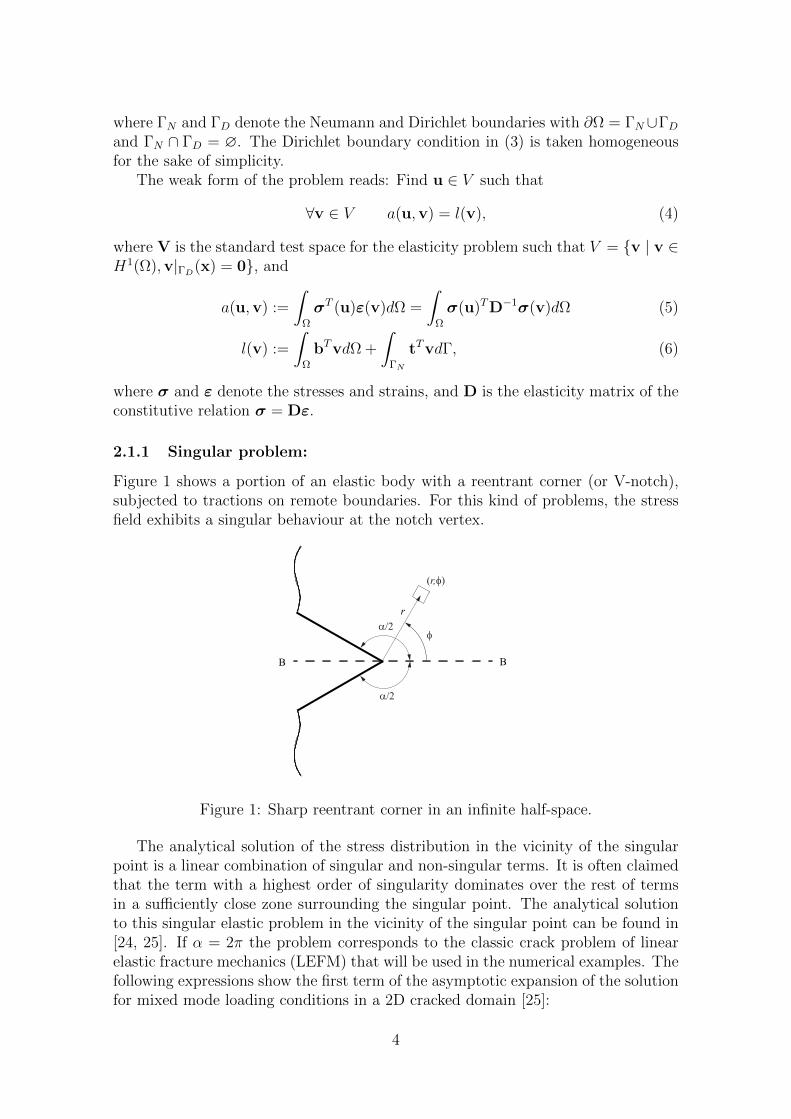
Figure 1 shows a portion of an elastic body with a reentrant corner (or V-notch),subjected to tractions on remote boundaries. For this kind of problems, the stressfield exhibits a singular behaviour at the notch vertex.
B
a/2
a/2
B
r
( )r,f
f
Figure 1: Sharp reentrant corner in an infinite half-space.
The analytical solution of the stress distribution in the vicinity of the singularpoint is a linear combination of singular and non-singular terms. It is often claimedthat the term with a highest order of singularity dominates over the rest of termsin a sufficiently close zone surrounding the singular point. The analytical solutionto this singular elastic problem in the vicinity of the singular point can be found in[24, 25]. If α = 2π the problem corresponds to the classic crack problem of linearelastic fracture mechanics (LEFM) that will be used in the numerical examples. Thefollowing expressions show the first term of the asymptotic expansion of the solutionfor mixed mode loading conditions in a 2D cracked domain [25]:
4

u1(r, φ) =KI
2µ
√r
2πcos
φ
2(κ− cosφ) +
KII
2µ
√r
2πsin
φ
2(2 + κ+ cosφ)
u2(r, φ) =KI
2µ
√r
2πsin
φ
2(κ− cosφ) +
KII
2µ
√r
2πcos
φ
2(2− κ− cosφ)
(7)
σ11(r, φ) =KI√2πr
cosφ
2
(1− sin
φ
2sin
3φ
2
)− KII√
2πrsin
φ
2
(2 + cos
φ
2cos
3φ
2
)σ22(r, φ) =
KI√2πr
cosφ
2
(1 + sin
φ
2sin
3φ
2
)+
KII√2πr
sinφ
2cos
φ
2cos
3φ
2
σ12(r, φ) =KI√2πr
sinφ
2cos
φ
2cos
3φ
2+
KII√2πr
cosφ
2
(1− sin
φ
2sin
3φ
2
) (8)
where KI and KII are the generalise stress intensity factors (GSIF) for modes Iand II. The GSIF are multiplicative constants that depend on the loading of theproblem and linearly determine the intensity of the displacement and stress fields inthe vicinity of the singular point.
2.2 Solution with FEM/XFEM.
Let uh be a finite element approximation to u such that uh(x) =∑
i∈I Ni(x)ui,where Ni represent the shape functions associated with node i and I is the set of allthe nodes in the mesh. The solution lies in a functional space V h ⊂ V associatedwith a mesh of isoparametric finite elements of characteristic size h, and it is suchthat
∀v ∈ V h a(uh,v) = l(v) (9)
Considering an XFEM formulation for the case of the singular problems of LEFMabove-mentioned, the FE approximation is enriched with Heaviside functions todescribe the discontinuity of the displacement field and with crack tip functions torepresent the asymptotic behaviour of the stress field near the crack tip. This avoidsthe need for a conforming mesh to describe the geometry of the crack [26] and theuse of adaptive techniques in order to capture the special features of the solution. Toensure the continuity of the solution, the partition of unity property of the classicallinear shape functions is used. Therefore, the XFEM displacements interpolation ina 2D model is given by:
uh(x) =∑i∈I
Ni(x)ai +∑j∈J
Nj(x)H(x)bj +∑m∈M
Nm(x)
(4∑`=1
F`(x)c`m
)(10)
where ai are the conventional nodal degrees of freedom, bj are the coefficients as-sociated with the discontinuous enrichment functions, and cm those associated withthe functions spanning the asymptotic field. In the above equation, I is the set ofall the nodes in the mesh, M is the subset of nodes enriched with crack tip func-tions, and J is the subset of nodes enriched with the discontinuous enrichment (see
5
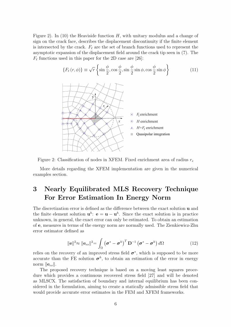
Figure 2). In (10) the Heaviside function H, with unitary modulus and a change ofsign on the crack face, describes the displacement discontinuity if the finite elementis intersected by the crack. F` are the set of branch functions used to represent theasymptotic expansion of the displacement field around the crack tip seen in (7). TheF` functions used in this paper for the 2D case are [26]:
F` (r, φ) ≡ √r
sinφ
2, cos
φ
2, sin
φ
2sinφ, cos
φ
2sinφ
(11)
e
l
l
y
Quasipolar integration
r
Figure 2: Classification of nodes in XFEM. Fixed enrichment area of radius re
More details regarding the XFEM implementation are given in the numericalexamples section.
3 Nearly Equilibrated MLS Recovery Technique
For Error Estimation In Energy Norm
The discretization error is defined as the difference between the exact solution u andthe finite element solution uh: e = u − uh. Since the exact solution is in practiceunknown, in general, the exact error can only be estimated. To obtain an estimationof e, measures in terms of the energy norm are normally used. The Zienkiewicz-Zhuerror estimator defined as
‖e‖2≈ ‖ees‖2=
∫Ω
(σ∗ − σh
)TD−1
(σ∗ − σh
)dΩ (12)
relies on the recovery of an improved stress field σ∗, which is supposed to be moreaccurate than the FE solution σh, to obtain an estimation of the error in energynorm ‖ees‖.
The proposed recovery technique is based on a moving least squares proce-dure which provides a continuous recovered stress field [27] and will be denotedas MLSCX. The satisfaction of boundary and internal equilibrium has been con-sidered in the formulation, aiming to create a statically admissible stress field thatwould provide accurate error estimates in the FEM and XFEM frameworks.
6

3.1 MLS recovery
The MLS technique is based on a weighted least squares formulation biased towardsthe test point where the value of the function is asked. The technique considers apolynomial expansion for each one of the components of the recovered stress field inthe form:
σ∗i (x) = p(x)ai(x) i = xx, yy, xy (13)
where p represents a polynomial basis and a are unknown coefficients
p(x) = 1 x y x2 xy y2 . . . (14)
ai(x) = a0i(x) a1i(x) a2i(x) a3i(x) a4i(x) a5i(x) . . .T (15)
For 2D, the expression to evaluate the recovered stress field reads:
σ∗(x) =
σ∗xx(x)σ∗yy(x)σ∗xy(x)
= P(x)A(x) =
p(x) 0 00 p(x) 00 0 p(x)
axx(x)ayy(x)axy(x)
(16)
The format of (16), considering the three components of the stress vector in asingle equation, will result useful to impose the constraints required to satisfy theequilibrium equations.
Suppose that χ is a point within Ωx, being Ωx the support corresponding to apoint x defined by a distance (radius) RΩx . The MLS approximation for each stresscomponent at χ is given by
σ∗i (x,χ) = p(χ)ai(x) ∀χ ∈ Ωx, i = xx, yy, xy (17)
To obtain the coefficients A we have adopted the Continuous Moving LeastSquares Approximation described in [27]. The following functional is minimised:
J(x) =
∫Ωx
W (x− χ)[σ∗ (x,χ)− σh (χ)
]2dχ (18)
Evaluating ∂J/∂A = 0 results in the linear system M(x)A(x) = G(x) used toevaluate A, where
M (x) =
∫Ωx
W (x− χ) PT (χ) P (χ) dχ
G (x) =
∫Ωx
W (x− χ) PT (χ)σh (χ) dχ
(19)
Assuming that there are n sampling points of coordinates χl (l = 1...n) withinthe support of x, with weight Hl and being |J(χl)| the jacobian determinant, theexpressions in (18, 19) can be numerically evaluated as
J(x) =n∑l=1
W (x− χl)[σ∗(x,χl)− σh(χl)]2|J(χl)|Hl
M (x) =n∑l=1
W (x− χl) PT (χl) P (χl) |J(χl)|Hl
G (x) =n∑l=1
W (x− χl) PT (χl)σh (χl) |J(χl)|Hl
(20)
7

The integration points for the numerical evaluation of the integrals in the aboveequations correspond to the integration points within Ωx used in the FE analysis, forwhich the stress field is already available. In (19) W is the MLS weighting function,which in this paper has been taken as the fourth-order spline, commonly used in theMLS related literature:
W (x− χ) =
1− 6s2 + 8s3 − 3s4 if |s| ≤ 1
0 if |s| > 1(21)
where s denotes the normalised distance function given by
s =‖x− χ‖RΩx
(22)
In the more commonly used Discrete MLS approach [27] the functional J (x)would be defined as:
J (x) =n∑l=1
W (x− χl)[σ∗ (x,χl)− σh (χl)
]2(23)
This approach would thus produce similar expressions to the equations shownin (20) with the difference that, in the continuous approach, each of the samplingpoints χl is weighted by its associated area |J(χl)|Hl. Our numerical experience hasshown that the Continuous MLS approximation used in this paper is more accuratethan the discrete approximation, especially when the distribution of the samplingpoints is not uniform within the support.
Continuity in σ∗ is directly provided by the MLS procedure previously describedbecause the weighting function W ensures that stress sampling points leave or enterthe support domain in a gradual and smooth manner when x moves [27]. Thefollowing sections are devoted to the satisfaction of the equilibrium equations.
3.2 Satisfaction of the boundary equilibrium equation
The boundary equilibrium equation must be satisfied at each point along the con-tour. In [23, 16, 8], where an SPR-based technique was used, the authors enforcedthe satisfaction of the boundary conditions in patches along the boundary usingLagrange Multipliers to impose the appropriate constraints between the unknowncoefficients to be evaluated. However, this approach produces discontinuities in aMLS formulation as we move from a support fully in the interior of the domain toa support intersecting the boundary.
In order to avoid the introduction of discontinuities in the recovered field, wehave followed a nearest point approach that introduces the exact satisfaction of theboundary equilibrium equation in a smooth continuous manner. As the constraintis smoothly introduced there is no jump when the support does not longer intersectsΓ. For a point x ∈ Ω whose support Ωx intersects the boundary Γ, the equilibriumconstraints are considered only in the closest points χj ∈ Γ on the boundaries within
8

the support of x, as shown in Figure 3. Note that we can have more than one nearestpoint for a given support, as is the case for a point x approaching a corner wherewe take one point for each side of the corner (see Figure 3). In this case, twodifferent points have to be considered on the boundary to avoid jumps induced bythe different boundary conditions when crossing the diagonal that bisects the corner.
Support centreBoundary closest pointsSampling points
Figure 3: MLS support with boundary conditions applied on the nearest boundarypoints.
Let us express the stress vector σ∗(x,χ) in a coordinate system xy aligned withthe contour at χj such that x is the outward normal vector, rotated an angle α withrespect to x:
σ∗(x,χ) = R(α)σ∗(x,χ) (24)
where R is the stress rotation matrix
R =
rxxryyrxy
=
cos2 α sin2 α sin(2α)sin2 α cos2 α − sin(2α)
− sin(2α)/2 sin(2α)/2 cos(2α)
(25)
The MLS functional expressed in its continuous version and incorporating theboundary constraints reads:
J(x) =n∑l=1
W (x− χl)[σ∗ (x,χl)− σh (χl)
]2 |J(χl)|Hl+
nbc∑j=1
W(x− χj
) [σ∗i
(x,χj
)− σex
i
(χj)]2
(26)
=n∑l=1
W (x− χl)[P (χl) A (x)− σh (χl)
]2 |J(χl)|Hl+
nbc∑j=1
W(x− χj
) [ri(α)P(χj)A (x)− σex
i
(χj)]2
i = xx, xy
9
where nbc is the number of points χj on the boundary where the known bound-ary constraints σex
i(in general, those would be the normal σxx and tangential
σxy stresses) are considered. Evaluating ∂J/∂A = 0 results in the linear systemM(x)A(x) = G(x) used to evaluate A, where, in this case
M =n∑l=1
W (x− χl) PT (χl) P (χl) |J(χl)|Hl+
nbc∑j=1
W (x− χj)PT (χj)rTiriP(χj) (27)
G =n∑l=1
W (x− χl) PT (χl)σh (χl) |J(χl)|Hl+
nbc∑j=1
W (x− χj)PT (χj)rTiσexi
(χj) (28)
In the previous equations W is a weighting function defined as:
W (x− χj) =W (x− χj)
s=
1
s− 6s+ 8s2 − 3s3 if |s| ≤ 1
0 if |s| > 1(29)
This function has two main characteristics:
1. W includes the weighting function W such that the term for the boundaryconstraint is introduced smoothly into the functional J(x). As a result, therecovered stress field will be continuous in Ω
2. W also includes s−1 such that the weight of the boundary constraint in J(x)increases as we approach the boundary (when x → χj s → 0), therefore σ∗
will tend to exactly satisfy boundary equilibrium as x → χj (see Figure 4).Note that to estimate the error using the numerical integration in (12), thevalue of σ∗ is never evaluated on the boundary (where s = 0) because theintegration points considered are always inside the elements.
3.3 Satisfaction of the internal equilibrium equation.
In addition to the enforcement of boundary equilibrium, we will also consider thesatisfaction of the internal equilibrium equation using the Lagrange Multipliers tech-nique. Thus, we will try to enforce the recovered stress field σ∗ to satisfy the internalequilibrium equation
∇ · σ∗ + b = 0 (30)
The spatial derivatives of σ∗, considering (16), are expressed as
∇ · σ∗ = (∇ ·P) A + P (∇ ·A) (31)
10

A
B
I
WA
G
tn
A
B
WB
G
tn
sn( )x
B,
Bc*
sn( )x
A,
Ac*
sn( )
Ix
A,c*
tn( )x
I
sn( )x
A,c*
sn( )
Ix
B,c*
tn( )x
I
I
sn( )x
B,c*
Figure 4: Satisfaction of boundary equilibrium. σ∗n (xA,χ) and σ∗n(xB,χ) are thevalues of σ∗ (x,χ), projected along the direction normal to boundary Γ at I, inthe supports ΩA and ΩB of the points A and B, whose nearest point on Γ is I. tnrepresents the normal tractions applied on Γ. Note that σ∗n (x,χI) 6= tn (xI) althoughσ∗n (xB,χI) is more accurate than σ∗n (xA,χI). Thus, as x → xI , σ
∗n (x,χI) →
tn (xI) and, similarly the value of the stresses evaluated at the center of the supportσ∗n (x,x)→ tn (xI)
The first terms in (31) can be directly evaluated differentiating the polynomialbasis. Previous works [19, 20, 21] have only considered the first term in the sat-isfaction of the appropriate equations, thus only providing a pseudo-satisfaction ofthese equations [21]. Therefore, the second term in (31) must also be obtained. Toevaluate it, we differentiate the linear system MA = G:
(∇ ·M) A + M (∇ ·A) = ∇ ·G (32)
Evaluating ∇ ·A from (32), replacing in (31) and expanding leads to:
∂σ∗
∂x=
(∂P
∂x−PM−1∂M
∂x
)A + PM−1∂G
∂x= E,xA + f ,x (33)
∂σ∗
∂y=
(∂P
∂y−PM−1∂M
∂y
)A + PM−1∂G
∂y= E,yA + f ,y (34)
where the partial derivatives of M and G with respect, for example, to x are
∂M
∂x=
n∑l=1
∂W (x− χl)∂x
PT (χl)P(χl)|J(χl)|Hl+
nbc∑j=1
∂W (x− χj)∂x
PT (χj)rTiriP(χj) (35)
∂G
∂x=
n∑l=1
∂W (x− χl)∂x
PT (χl)σh(χl)|J(χl)|Hl+
nbc∑j=1
∂W (x− χj)∂x
PT (χj)rTiσexi
(χj) (36)
11

where, differentiating (21, 29),
∂W (x− χ)
∂x=∂W (x− χ)
∂s
∂s
∂x(37)
∂W(x− χj
)∂x
=∂W
(x− χj
)∂s
∂s
∂x(38)
In these equations ∂s/∂x can be obtained from (22) or, alternatively, from (43)for the case shown in the next section. Equations (33, 34) are expressed as a functionof A, so, we can write the two terms of the internal equilibrium equation (30) as afunction of the vector of unknowns A:
∂σ∗xx∂x
+∂σ∗xy∂y
+ bx = (Exx,x + Exy,y) A + (fxx,x + fxy,y) + bx = 0 (39)
∂σ∗xy∂x
+∂σ∗yy∂y
+ by = (Exx,y + Eyy,y) A + (fxy,x + fyy,y) + by = 0 (40)
where i,j (i = xx, yy, xy and j = x, y) represents the row in ,j correspondingto the ith component of the stresses. These expressions define the constraints be-tween the coefficients A required to satisfy the internal equilibrium equation at x.Lagrange Multipliers are used to impose these constraint equations.
The use of the Lagrange Multipliers technique to impose the equilibrium con-straint (39, 40) in (26) leads to the following system of equations:[
M CT
C 0
] [Aλ
]=
[GD
](41)
where C and D are the terms used to impose the constraint equations and λ is thevector of Lagrange Multipliers.
However, in (32) it was assumed that A is evaluated solving MA = G, although,operating by blocks in (41) the following system of equations is obtained:
MA + CTλ = G (42)
Hence, in the formulation proposed in this paper we have neglected the term CTλwhen evaluating the partial derivatives of A. Evidently, this implies that the internalequilibrium equation is not fully satisfied, leading to a nearly exact satisfaction ofthe internal equilibrium equation. As described in the numerical examples, thisapproximation represents an enhancement with respect to the pseudo satisfactionof equilibrium [21].
References [23, 28] show that the error estimator in (12) would produce an uppererror bound if σ∗ is statically admissible. The MLSCX recovery technique producesa continuous stress field where the internal equilibrium equation is not fully satisfied.Hence σ∗ is continuous and nearly equilibrated and, thus, nearly statically admis-sible. Therefore, although the error estimate provided by the proposed recoverytechnique is very sharp, it is not a guaranteed upper error bound.
12
3.4 Visibility
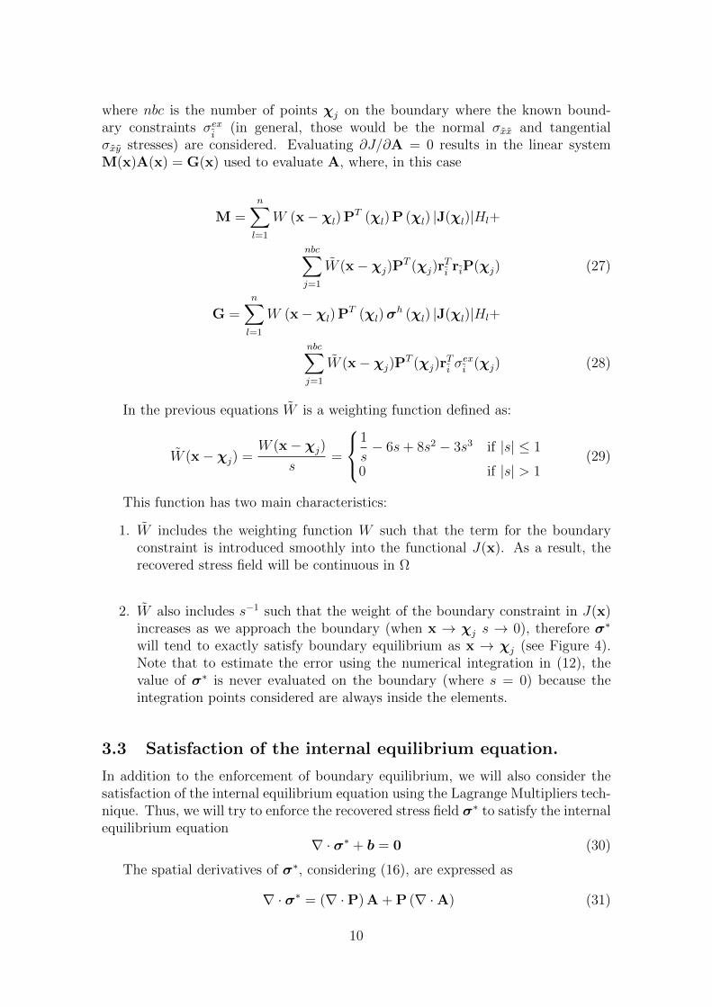
For problems with re-entrant corners a visibility criterion is used to modify thenormalised distance s in (22). The standard weight function depends on the distancebetween the central point of the support and the sampling points, decreasing as thesampling points are located farther from the centre [5].
Consider a domain with a re-entrant corner as shown in Figure 5. The valueof the weight function for a sampling point χl, considering a centre point x whosesupport contains the singularity at χλ, diminishes with the visibility of χl from xsuch that, for points that cannot be directly viewed from x, instead of (22), thefollowing equation is used
s =‖x− χλ‖+ ‖χl − χλ‖
RΩx
(43)
Figure 5: Domain with re-entrant corner.
3.5 Stress splitting for singular problems.
It is well known that smoothing techniques perform badly when the solution containsa singularity. In [7, 29] a technique that decomposes the stress field in singular andsmooth parts in order to improve the accuracy of SPR-based error estimators wasproposed. The authors indicated that the exact stress field σ corresponding to asingular problem can be expressed as the contribution of a smooth stress field, σsmo,and a singular stress field, σsing
σ = σsmo + σsing (44)
Hence, the recovered stress field for this kind of problems can be expressed asthe contribution of a smooth and a singular recovered stress fields
σ∗ = σ∗smo + σ∗sing (45)
To obtain an accurate approximation of the singular part we use the interactionintegral, as shown in [30], to compute a good estimation of the GSIFs KI and KII.Then, using the estimated values K∗I and K∗II we can evaluate a singular recoveredstress field σ∗sing from (8).
Assuming that σ∗sing is a good approximation of the singular part σsing, a FE-type representation of the smooth part σhsmo is given by
σhsmo = σh − σ∗sing (46)
13

In [7, 29] an SPR-based recovery technique was used to smooth the discontin-uous stress field σhsmo. In this paper, we use the moving least squares procedurepreviously described to recover the smooth part of the solution σ∗smo. In [7, 29]the stress splitting procedure was only used in a small area around the crack tip.In the procedure proposed herein the stress splitting is used in the whole domainof the problem in order to avoid discontinuities along the blending zone. Thus, theboundary tractions to be considered for the satisfaction of the boundary equilibriumequation in the smooth problem are:
tsmo = t− t∗sing (47)
where t∗sing are the projection of σ∗sing. It must be taken into account that thecrack faces are treated as any other Neumann boundary where satisfaction of theboundary equilibrium equation will be imposed.
Note that σ∗sing is equilibrated and continuous, therefore, the resulting recoveredstress field σ∗ = σ∗sing + σ∗smo only has small lacks of internal equilibrium in σ∗smoinduced by the recovery process.
3.6 Adaptive strategy
The refinement of the mesh using the error estimate as the guiding parameter con-siders an stopping criterion that checks the value of the estimated error against aprescribed or desired error. If the estimated error is higher than the desired errorthen the mesh is refined. Several procedures to perform the refinement are availablein the literature. To define the size of the elements in the new mesh we follow theadaptive process described in [31, 32, 33] which minimises the number of elementsin the new mesh. This criterion is equivalent to the traditional approach of equallydistributing the error in each element of the new mesh as proven in [34, 35].
4 Numerical Examples
In this section numerical tests using 2D benchmark problems with exact solutionare used to investigate the quality of the proposed error estimation technique. Thefirst three problems (smooth and singular) consider a FEM approximation whilstthe fourth problem is solved using an XFEM formulation. For all the models weassume a plane strain condition. Sequences of meshes with linear (TRI3), quadratic(TRI6) triangles and linear (QUAD4), quadratic (QUAD8) quadrilaterals elementsare considered for the analyses. Uniform and h-adaptive refinements have beenused. The h-adaptive refinement is based on element splitting using multipointconstraints (MPC) to impose C0 continuity at hanging nodes. Quadrature rules of1, 3, 2 × 2 and 3 × 3 Gauss points are used for TRI3, TRI6, QUAD4 and QUAD8elements, respectively. A support size with a radius two times the average sizeof the surrounding elements is used to perform the MLS recovery. 19 samplingpoints in triangular elements and 25 sampling points in quadrilaterals are used foran accurate numerical evaluation of (12) in order to avoid the effect of numericalerrors due to integration. The computational cost of the proposed technique could
14

be alleviated by evaluating (12) using quadrature rules with fewer integration pointsat the expense of introducing errors due to integration in the procedure. The MLSbasis functions used in the recovery are polynomials p one order higher than thecorresponding FE displacement basis.
The performance of the technique is evaluated using the effectivity index of theerror in energy norm, both at global and local levels. Globally, we consider the valueof the effectivity index θ given by
θ =‖ees‖‖e‖ (48)
where ‖e‖ denotes the exact error in energy norm, and ‖ees‖ represents the evaluatederror estimate. At element level, the distribution of the local effectivity index D, itsmean value m(|D|) and standard deviation σ(D) is analysed, as described in [7]:
D = θe − 1 if θe ≥ 1
D = 1− 1
θeif θe < 1
with θe =‖eees‖‖ee‖ (49)
where superscript e denotes evaluation at element level.The h-adaptive refinement procedure considering the error in quantities of inter-
est is implemented based on previous adaptive procedures using the error in energynorm. The technique aims to minimise the number of elements to get the targeterror by equally distributing the element error in the mesh.
4.1 2×2 square with a 3rd-order polynomial solution
The 2×2 square model shown in Figure 6 is analysed, with material parametersE = 1000 for the Young’s modulus and ν = 0.3 for the Poisson’s ratio. Dirichletboundary conditions are indicated in the figure. The problem is defined such thatthe exact displacement solution is given by
u(x, y) = x+ x2 − 2xy + x3 − 3xy2 + x2y (50)
v(x, y) = −y − 2xy + y2 − 3x2y + y3 − xy2 (51)
The exact values of the stress components are applied along the Neumann bound-ary denoted by a dashed line in Figure 6. These stresses can be derived from theexact displacement field under plane strain condition, and read
σxx =E
1 + ν(1 + 2x− 2y + 3x2 − 3y2 + 2xy) (52)
σyy =E
1 + ν(−1− 2x+ 2y − 3x2 + 3y2 − 2xy) (53)
σxy =E
1 + ν(−x− y +
x2
2− y2
2− 6xy) (54)
The following body forces must be applied to satisfy equilibrium:
bx(x, y) = − E
1 + ν(1 + y) (55)
by(x, y) = − E
1 + ν(1− x) (56)
15

2
2
x
y
Figure 6: 2×2 square plate.
We have used this problem to analyse the influence of different implementationsof the MLS recovery technique in the error estimate, considering the following cases:
• MLS: Plain Moving Least Squares recovery
• MLS+BE: MLS technique with the boundary equilibrium enhancement de-scribed in Section 3.2
• MLS+BE+PIE: MLS technique with the boundary equilibrium enhance-ment described in Section 3.2 and the pseudo satisfaction of the internal equi-librium equation
• MLSCX: Technique proposed in this paper
The results for the plain MLS case will be used as reference. The other three casesrepresent implementations which increasingly approach the full satisfaction of theequilibrium equations. Figures 7 to 10 show the effectivity of the error estimationvs. the number of degrees of freedom (dof) using these four implementations forh-adaptive meshes.
These figures clearly show that the satisfaction of boundary equilibrium (curvesMLS+BE) plays the most important role towards the enforcement of equilibriumand, therefore, an improvement on the accuracy of the error estimator when com-pared with the MLS curve. The additional pseudo-satisfaction of internal equi-librium (curves MLS+BE+PEI) does not improve, and sometimes provides worseeffectivities than boundary equilibrium constraints, as it can be seen in Figure 10.From Figures 7 to 10 we can see an increase in the accuracy for the MLSCX curveswith respect to the other curves, with effectivities very close to θ = 1.
Figure 11 shows the evolution with respect to mesh refinement of the globaleffectivity index θ, the mean absolute value m(|D|) and standard deviation σ(D)of the local effectivity index for the different types of elements considered. Notethat with the proposed technique we obtain very accurate values of θ and the error
16

102 1030.88
0.9
0.92
0.94
0.96
0.98
1
dof
θ
MLSMLS+BEMLS+BE+PIEMLSCX
MLS MLS+BEdof θ dof θ102 0.886 102 0.987332 0.940 322 0.985
1180 0.968 1158 0.9904296 0.984 4192 0.996
MLS+BE+PIE MLSCXdof θ dof θ102 0.992 102 0.992322 0.987 326 0.991
1154 0.991 1168 0.9964220 0.995 4222 0.998
Figure 7: 2 × 2 square with h-adaptive meshes and TRI3 elements. Evolution of θfor different recoveries
103 104
0.97
0.98
0.99
1
dof
θ
MLSMLS+BEMLS+BE+PIEMLSCX
MLS MLS+BEdof θ dof θ366 0.966 366 0.993
1076 0.977 1068 0.9873120 0.988 3068 0.9938204 0.992 7920 0.996
MLS+BE+PIE MLSCXdof θ dof θ366 0.992 366 0.996
1068 0.987 1068 0.9903038 0.992 3038 0.9947866 0.996 7956 0.997
Figure 8: 2 × 2 square with h-adaptive meshes and TRI6 elements. Evolution of θfor different recoveries.
estimate converges to the exact value with the increase of the number of degrees offreedom. For this example, the best results are obtained with quadratic elements.
Figure 12 shows the distribution of the local effectivity on a set of TRI3 meshes,Figure 13 displays the same results for a set of QUAD4 meshes. In both cases we canobserve a quite homogeneous distribution of the local effectivity inside the domainand good results along the boundary of the problem. In addition, D decreases forfiner meshes and we always have values within a very narrow range. Figures 14 and15 show a similar behaviour for quadratic elements.
4.2 Thick-wall cylinder subjected to an internal pressure.
The geometrical model for this problem is shown in Figure 16. Due to symmetryconditions, only one part of the section is modelled.
The exact solution for this problem is given by the following expressions. For apoint (x, y), c = b/a, r =
√x2 + y2 the radial displacement is given by
ur =P (1 + ν)
E(c2 − 1)
(r (1− 2ν) +
b2
r
)(57)
17

102 1030.85
0.9
0.95
1
dof
θ
MLSMLS+BEMLS+BE+PIEMLSCX
MLS MLS+BEdof θ dof θ102 0.858 102 0.985326 0.922 296 0.993
1050 0.955 964 0.9983498 0.975 3108 0.999
MLS+BE+PIE MLSCXdof θ dof θ102 0.989 102 1.001296 0.992 302 1.001964 0.997 960 1.003
3108 0.999 3024 1.001
Figure 9: 2× 2 square with h-adaptive meshes and QUAD4 elements. Evolution ofθ for different recoveries
102.5 103 103.5
0.97
0.98
0.99
1
dof
θ
MLSMLS+BEMLS+BE+PIEMLSCX
MLS MLS+BEdof θ dof θ286 0.967 286 0.993702 0.974 684 0.993
1664 0.983 1624 0.9964344 0.981 4344 0.995
MLS+BE+PIE MLSCXdof θ dof θ286 0.994 286 1.000684 0.991 702 1.000
1624 0.994 1642 1.0004362 0.993 4354 1.000
Figure 10: 2 × 2 square with h-adaptive meshes and QUAD8 elements. Evolutionof θ for different recoveries.
102 103 104
0.995
1
1.005
dof
θ
TRI3QUAD4TRI6QUAD8
TRI3 QUAD4dof θ dof θ102 0.992 102 1.001366 0.993 366 1.001
1374 0.994 1374 1.0025310 0.997 5310 1.001
TRI6 QUAD8dof θ dof θ366 0.996 286 1.000
1374 0.998 1054 1.0015310 0.999 4030 1.001
20862 0.999 15742 1.000
Figure 11: 2× 2 square with uniformly refined meshes. Evolution of the effectivityindex θ for different element types.
Stresses in cylindrical coordinates are
18
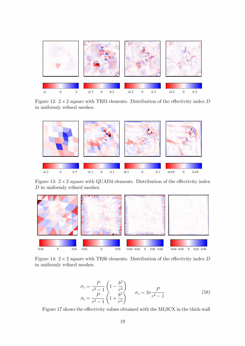
Figure 12: 2× 2 square with TRI3 elements. Distribution of the effectivity index Din uniformly refined meshes.
Figure 13: 2× 2 square with QUAD4 elements. Distribution of the effectivity indexD in uniformly refined meshes.
−0.05 0 0.05
−0.05 0 0.05
−0.04−0.02 0 0.02 0.04
−0.04−0.02 0 0.02 0.04
Figure 14: 2× 2 square with TRI6 elements. Distribution of the effectivity index Din uniformly refined meshes.
σr =P
c2 − 1
(1− b2
r2
)σt =
P
c2 − 1
(1 +
b2
r2
) σz = 2νP
c2 − 1(58)
Figure 17 shows the effectivity values obtained with the MLSCX in the thick-wall
19
−0.01 0 0.01
−0.02−0.01 0 0.01 0.02
−0.01 0 0.01
−0.02 −0.01 0 0.01 0.02
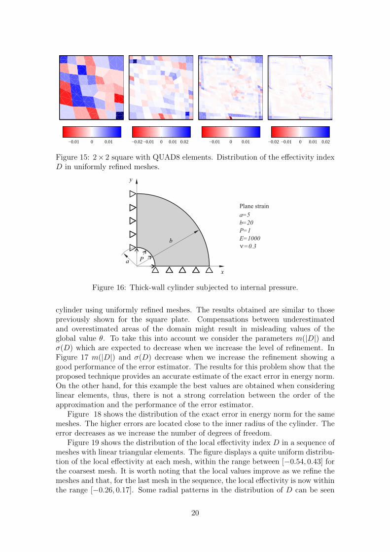
Figure 15: 2× 2 square with QUAD8 elements. Distribution of the effectivity indexD in uniformly refined meshes.
Plane strain
a=5b=20P=1E=1000 =0.3
b
y
x
a P
Figure 16: Thick-wall cylinder subjected to internal pressure.
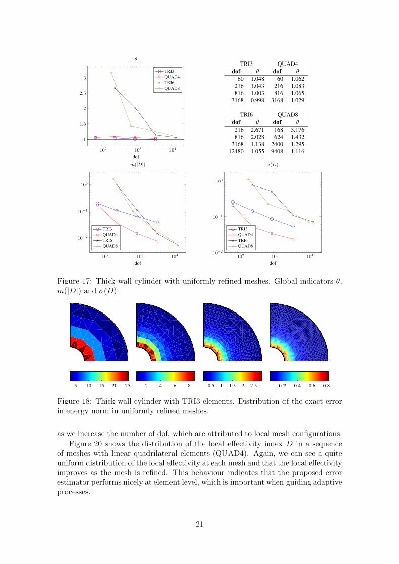
cylinder using uniformly refined meshes. The results obtained are similar to thosepreviously shown for the square plate. Compensations between underestimatedand overestimated areas of the domain might result in misleading values of theglobal value θ. To take this into account we consider the parameters m(|D|) andσ(D) which are expected to decrease when we increase the level of refinement. InFigure 17 m(|D|) and σ(D) decrease when we increase the refinement showing agood performance of the error estimator. The results for this problem show that theproposed technique provides an accurate estimate of the exact error in energy norm.On the other hand, for this example the best values are obtained when consideringlinear elements, thus, there is not a strong correlation between the order of theapproximation and the performance of the error estimator.
Figure 18 shows the distribution of the exact error in energy norm for the samemeshes. The higher errors are located close to the inner radius of the cylinder. Theerror decreases as we increase the number of degrees of freedom.
Figure 19 shows the distribution of the local effectivity index D in a sequence ofmeshes with linear triangular elements. The figure displays a quite uniform distribu-tion of the local effectivity at each mesh, within the range between [−0.54, 0.43] forthe coarsest mesh. It is worth noting that the local values improve as we refine themeshes and that, for the last mesh in the sequence, the local effectivity is now withinthe range [−0.26, 0.17]. Some radial patterns in the distribution of D can be seen
20
102 103 104
1
1.5
2
2.5
3
dof
θ
TRI3QUAD4TRI6QUAD8
TRI3 QUAD4dof θ dof θ
60 1.048 60 1.062216 1.043 216 1.083816 1.003 816 1.065
3168 0.998 3168 1.029
TRI6 QUAD8dof θ dof θ216 2.671 168 3.176816 2.028 624 1.432
3168 1.138 2400 1.29512480 1.055 9408 1.116
102 103 104
10−2
10−1
100
dof
m(|D|)
TRI3QUAD4TRI6QUAD8
102 103 10410−2
10−1
100
dof
σ(D)
TRI3QUAD4TRI6QUAD8
Figure 17: Thick-wall cylinder with uniformly refined meshes. Global indicators θ,m(|D|) and σ(D).
5 10 15 20 25 2 4 6 8 0.5 1 1.5 2 2.5 0.2 0.4 0.6 0.8
Figure 18: Thick-wall cylinder with TRI3 elements. Distribution of the exact errorin energy norm in uniformly refined meshes.
as we increase the number of dof, which are attributed to local mesh configurations.Figure 20 shows the distribution of the local effectivity index D in a sequence
of meshes with linear quadrilateral elements (QUAD4). Again, we can see a quiteuniform distribution of the local effectivity at each mesh and that the local effectivityimproves as the mesh is refined. This behaviour indicates that the proposed errorestimator performs nicely at element level, which is important when guiding adaptiveprocesses.
21

Figure 19: Thick-wall cylinder with TRI3 elements. Distribution of the effectivityindex D in uniformly refined meshes.
Figure 20: Thick-wall cylinder with QUAD4 elements. Distribution of the effectivityindex D in uniformly refined meshes.
4.2.1 Influence of support size.
One of the parameters that affects the performance of the proposed error estimator isthe radius RΩx that defines the MLS support at a point x, also known as the domainof influence. The idea is to define a support with a number of sampling points largeenough to be able to solve the MLS fitting and to obtain an accurate polynomialexpansion of the stresses, but not too large that we risk excessively smoothing thestress field and no longer describing the local behaviour of the solution. Moreover,larger supports means more computational effort as more sampling points should beconsidered.
In order to fix the domain of influence at a particular point we first evaluate theaverage size of the elements surrounding each node of the mesh. Then, we definethe radius of the support at nodes as RΩx(xi) = k l(xi) where k is a constant thattakes positive values and l(xi) is the average size of the elements containing node i.Once the value of RΩx is evaluated at nodes, the value of RΩx at any point x withinan element is interpolated from the nodes using the displacement shape functions.Note that as RΩx is a function of x. Its definition has been used in the derivativesof s defined in (22) (or alternatively in (43)) required for the evaluation of (37, 38).
Figure 21 shows the global results for a sequence of TRI3 elements considering
22

different values of k. Figure 22 shows the same results for QUAD4 meshes. Notethat for small supports the values of the local indicators are less accurate even if thevalues for the global indicator are closer to one. A good balance between accuracyand local definition of the smoothing function is obtained for k = 2, which is thevalue considered in the examples presented herein.
102 103
1
1.02
1.04
1.06
1.08
dof
θ
k = 1
k = 1.5
k = 2
k = 2.5
102 10310−1.5
10−1
10−0.5
dof
m(|D|)
k = 1
k = 1.5
k = 2
k = 2.5
102 10310−2
10−1
dof
σ(D)
k = 1
k = 1.5
k = 2
k = 2.5
Figure 21: Thick-wall cylinder with uniformly refined TRI3 meshes. Global indica-tors θ, m(|D|) and σ(D) for different values of k.
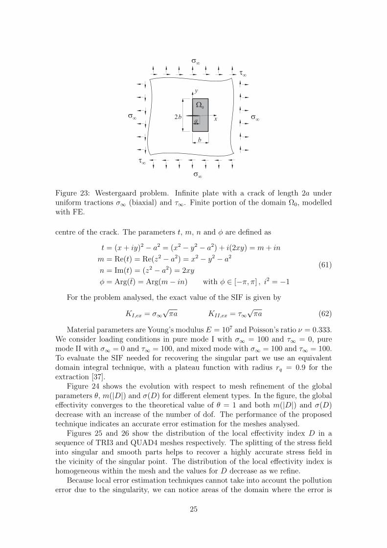
4.3 Westergaard problem – FEM solution.
To evaluate the performance of the proposed technique for singular problems weconsider the Westergaard problem [7, 36] as it has an exact analytical solution. TheWestergaard problem corresponds to an infinite plate loaded at infinity with biaxialtractions σx∞ = σy∞ = σ∞ and shear traction τ∞, presenting a crack of length 2a asshown in Figure 23. Combining the externally applied loads we can obtain differentloading conditions: pure mode I, pure mode II or mixed mode.
The numerical model corresponds to a finite portion of the domain (a = 1 andb = 4 in Figure 23). The applied projected stresses for mode I are evaluated fromthe analytical Westergaard solution [36]:
23

102 103
0.95
1
1.05
1.1
1.15
dof
θ
k = 1
k = 1.5
k = 2
k = 2.5
102 103
10−2
10−1
dof
m(|D|)
k = 1
k = 1.5
k = 2
k = 2.5
102 10310−2
10−1
dof
σ(D)
k = 1
k = 1.5
k = 2
k = 2.5
Figure 22: Thick-wall cylinder with uniformly refined QUAD4 meshes. Global indi-cators θ, m(|D|) and σ(D) for different values of k.
σIx(x, y) =σ∞√|t|
[(x cos
φ
2− y sin
φ
2
)+ y
a2
|t|2(m sin
φ
2− n cos
φ
2
)]σIy(x, y) =
σ∞√|t|
[(x cos
φ
2− y sin
φ
2
)− y a
2
|t|2(m sin
φ
2− n cos
φ
2
)]τ Ixy(x, y) = y
a2σ∞
|t|2√|t|
(m cos
φ
2+ n sin
φ
2
) (59)
and for mode II:
σIIx (x, y) =τ∞√|t|
[2
(y cos
φ
2+ x sin
φ
2
)− y a
2
|t|2(m cos
φ
2+ n sin
φ
2
)]σIIy (x, y) = y
a2τ∞
|t|2√|t|
(m cos
φ
2+ n sin
φ
2
)τ IIxy (x, y) =
τ∞√|t|
[(x cos
φ
2− y sin
φ
2
)+ y
a2
|t|2(m sin
φ
2− n cos
φ
2
)] (60)
where the stress fields are expressed as a function of x and y, with origin at the
24
2ba
y
x
W0
b
s¥
t¥
t¥
s¥
s¥ s
¥
Figure 23: Westergaard problem. Infinite plate with a crack of length 2a underuniform tractions σ∞ (biaxial) and τ∞. Finite portion of the domain Ω0, modelledwith FE.
centre of the crack. The parameters t, m, n and φ are defined as
t = (x+ iy)2 − a2 = (x2 − y2 − a2) + i(2xy) = m+ in
m = Re(t) = Re(z2 − a2) = x2 − y2 − a2
n = Im(t) = (z2 − a2) = 2xy
φ = Arg(t) = Arg(m− in) with φ ∈ [−π, π] , i2 = −1
(61)
For the problem analysed, the exact value of the SIF is given by
KI,ex = σ∞√πa KII,ex = τ∞
√πa (62)
Material parameters are Young’s modulus E = 107 and Poisson’s ratio ν = 0.333.We consider loading conditions in pure mode I with σ∞ = 100 and τ∞ = 0, puremode II with σ∞ = 0 and τ∞ = 100, and mixed mode with σ∞ = 100 and τ∞ = 100.To evaluate the SIF needed for recovering the singular part we use an equivalentdomain integral technique, with a plateau function with radius rq = 0.9 for theextraction [37].
Figure 24 shows the evolution with respect to mesh refinement of the globalparameters θ, m(|D|) and σ(D) for different element types. In the figure, the globaleffectivity converges to the theoretical value of θ = 1 and both m(|D|) and σ(D)decrease with an increase of the number of dof. The performance of the proposedtechnique indicates an accurate error estimation for the meshes analysed.
Figures 25 and 26 show the distribution of the local effectivity index D in asequence of TRI3 and QUAD4 meshes respectively. The splitting of the stress fieldinto singular and smooth parts helps to recover a highly accurate stress field inthe vicinity of the singular point. The distribution of the local effectivity index ishomogeneous within the mesh and the values for D decrease as we refine.
Because local error estimation techniques cannot take into account the pollutionerror due to the singularity, we can notice areas of the domain where the error is
25

103 104
0.85
0.9
0.95
1
dof
θ
TRI3QUAD4TRI6QUAD8
TRI3 QUAD4dof θ dof θ653 0.846 653 0.914927 0.937 879 0.970
2017 0.961 1905 0.9885835 0.983 5871 0.999
TRI6 QUAD8dof θ dof θ2459 0.941 1883 0.9412983 0.973 2343 0.9624749 0.987 3739 0.986
10391 0.990 7727 0.991
103 104
10−1
100
101
dof
m(|D|)
TRI3QUAD4TRI6QUAD8
103 104
10−1
100
101
dof
σ(D)
TRI3QUAD4TRI6QUAD8
Figure 24: Westergaard problem under mode I with FEM h-adapted meshes. Globalindicators θ, m(|D|) and σ(D).
underestimated in this example, especially in the first meshes. The effect of pollutionerror is partially overcome by the use of h-adaptive refinement (or enriched meshesas it is shown in the next section).
4.4 Westergaard problem – XFEM solution.
Let us now consider the Westergaard problem from the previous section, solvedusing an enriched finite element approximation. In the numerical analyses, we usea geometrical enrichment defined by a circular fixed enrichment area B(x0, re) withradius re = 0.5, with its centre at the crack tip x0 as proposed in [38]. For theextraction of the SIF we define a plateau function with radius rq = 0.9 as in theFEM case. Bilinear elements are considered in the models. For the numericalintegration of standard elements we use a 2 × 2 Gaussian quadrature rule. Theelements intersected by the crack are split into triangular integration subdomainsthat do not contain the crack. Alternatives which do not require this subdivisionare proposed in [39, 40]. We use 7 Gauss points in each triangular subdomain, anda 5×5 quasipolar integration in the subdomains of the element containing the cracktip [38], see Figure 2. We do not consider correction for blending elements. Methodsto address blending errors are proposed in [41, 42, 43, 44].
Figure 27 shows the evolution with respect to mesh refinement of the global
26
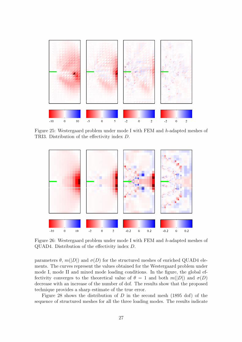
Figure 25: Westergaard problem under mode I with FEM and h-adapted meshes ofTRI3. Distribution of the effectivity index D.
Figure 26: Westergaard problem under mode I with FEM and h-adapted meshes ofQUAD4. Distribution of the effectivity index D.
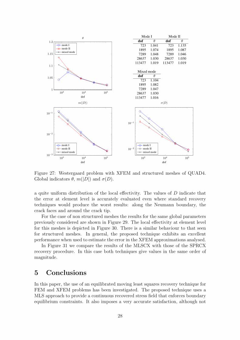
parameters θ, m(|D|) and σ(D) for the structured meshes of enriched QUAD4 ele-ments. The curves represent the values obtained for the Westergaard problem undermode I, mode II and mixed mode loading conditions. In the figure, the global ef-fectivity converges to the theoretical value of θ = 1 and both m(|D|) and σ(D)decrease with an increase of the number of dof. The results show that the proposedtechnique provides a sharp estimate of the true error.
Figure 28 shows the distribution of D in the second mesh (1895 dof) of thesequence of structured meshes for all the three loading modes. The results indicate
27
103 104 1051
1.05
1.1
1.15
1.2
dof
θ
mode Imode IImixed mode
Mode I Mode IIdof θ dof θ
723 1.041 723 1.1351895 1.074 1895 1.0877289 1.048 7289 1.046
28637 1.030 28637 1.030113477 1.019 113477 1.019
Mixed modedof θ
723 1.1041895 1.0827289 1.047
28637 1.030113477 1.016
103 104 10510−3
10−2
10−1
dof
m(|D|)
mode Imode IImixed mode
103 104 105
10−2
10−1
dof
σ(D)
mode Imode IImixed mode
Figure 27: Westergaard problem with XFEM and structured meshes of QUAD4.Global indicators θ, m(|D|) and σ(D).
a quite uniform distribution of the local effectivity. The values of D indicate thatthe error at element level is accurately evaluated even where standard recoverytechniques would produce the worst results: along the Neumann boundary, thecrack faces and around the crack tip.
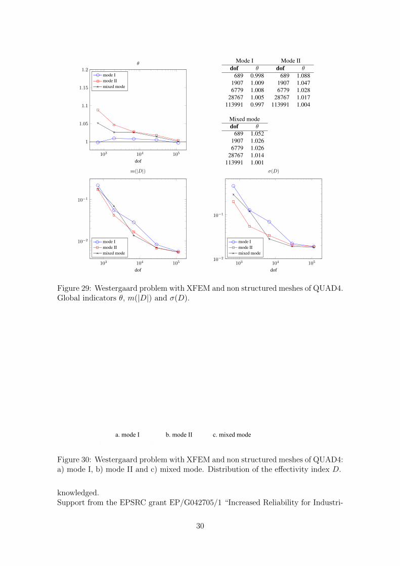
For the case of non structured meshes the results for the same global parameterspreviously considered are shown in Figure 29. The local effectivity at element levelfor this meshes is depicted in Figure 30. There is a similar behaviour to that seenfor structured meshes. In general, the proposed technique exhibits an excellentperformance when used to estimate the error in the XFEM approximations analysed.
In Figure 31 we compare the results of the MLSCX with those of the SPRCXrecovery procedure. In this case both techniques give values in the same order ofmagnitude.
5 Conclusions
In this paper, the use of an equilibrated moving least squares recovery technique forFEM and XFEM problems has been investigated. The proposed technique uses aMLS approach to provide a continuous recovered stress field that enforces boundaryequilibrium constraints. It also imposes a very accurate satisfaction, although not
28

a. mode I b. mode II c. mixed mode
Figure 28: Westergaard problem with XFEM and structured meshes of QUAD4: a)mode I, b) mode II and c) mixed mode. Distribution of the effectivity index D.
fully exact, of the internal equilibrium equation. Moreover, for singular problems itdecomposes the stress field into two different parts, singular and smooth, in order toenable the technique to describe the singular behaviour of the solution. A visibilitycriterion is used near reentrant corners and cracks to properly define the weight ofthe sampling points within the support.
The technique presented here has been validated using four different exampleswith known analytical solution. The numerical results have shown the accuracy ofthe proposed technique, which provides values of the effectivity index that convergeand are very close to the theoretical value θ = 1. The distribution of the localeffectivity at the elements is homogeneous for the tests considered, and the meanvalue m(|D|) and standard deviation σ(D) decrease as we increase the number ofdof. The obtained MLS recovered field is not fully statically admissible, thus, theprocedure does not guarantee the upper bound property. For this reason, it nearlybounds the exact error but not always yields an effectivity index greater than one,as clearly seen in the first example. In any case, the numerical results show that forthe examples presented the proposed technique yields sharp error estimates, whichare very accurate when compared with previous MLS approaches. Extension of thiswork to 3D problems is feasible given that the SIF along the crack front is evaluatedwith sufficient accuracy. It is known that in 3D problems the evaluation of the SIFis less accurate. In [7] the influence of the accuracy in the evaluation of the SIF inthe error estimator is investigated.
6 Acknowledgements
This work has been carried within the framework of the research project DPI2010-20542 of the Ministerio de Ciencia y e Innovacion y (Spain). The financial supportof the Universitat Politecnica de Valencia and Generalitat Valenciana is also ac-
29
103 104 105
1
1.05
1.1
1.15
1.2
dof
θ
mode Imode IImixed mode
Mode I Mode IIdof θ dof θ
689 0.998 689 1.0881907 1.009 1907 1.0476779 1.008 6779 1.028
28767 1.005 28767 1.017113991 0.997 113991 1.004
Mixed modedof θ
689 1.0521907 1.0266779 1.026
28767 1.014113991 1.001
103 104 105
10−2
10−1
dof
m(|D|)
mode Imode IImixed mode
103 104 10510−2
10−1
dof
σ(D)
mode Imode IImixed mode
Figure 29: Westergaard problem with XFEM and non structured meshes of QUAD4.Global indicators θ, m(|D|) and σ(D).
a. mode I b. mode II c. mixed mode
Figure 30: Westergaard problem with XFEM and non structured meshes of QUAD4:a) mode I, b) mode II and c) mixed mode. Distribution of the effectivity index D.
knowledged.Support from the EPSRC grant EP/G042705/1 “Increased Reliability for Industri-
30

103 104 105
1
1.05
1.1
1.15
1.2
dof
θ
MLSCXSPRCX
103 104 105
1
1.05
1.1
1.15
1.2
dof
θ
MLSCXSPRCX
103 104 1050.95
1
1.05
1.1
1.15
1.2
dof
θ
MLSCXSPRCX
Figure 31: Westergaard problem with XFEM and structured meshes of QUAD4.Effectivity index θ for the MLSCX and SPRCX recovery techniques.
ally Relevant Automatic Crack Growth Simulation with the eXtended Finite Ele-ment Method” is acknowledged.
References
[1] Ainsworth M, Oden JT. A posteriori Error Estimation in Finite Element Anal-ysis. John Wiley & Sons: Chichester, 2000.
[2] Bangerth W, Rannacher R. Adaptive Finite Element Methods for DifferentialEquations. ETH, Zurich, Birkhauser: Basel, 2003.
[3] de Almeida JPM, Pereira OJBA. Upper bounds of the error in local quanti-ties using equilibrated and compatible finite element solutions for linear elasticproblems. Computer Methods in Applied Mechanics and Engineering 1/15 2006;195(4-6):279–296.
[4] Moes N, Dolbow J, Belytschko T. A finite element method for crack growthwithout remeshing. International Journal for Numerical Methods in Engineer-ing 1999; 46(1):131–150, doi:10.1002/(SICI)1097-0207(19990910)46:1$〈$131::AID-NME726$〉$3.0.CO;2-J.
31

[5] Bordas S, Duflot M. Derivative recovery and a posteriori error estimate forextended finite elements. Computer Methods in Applied Mechanics and Engi-neering 07/15 2007; 196(35-36):3381–3399.
[6] Duflot M, Bordas S. A posteriori error estimation for extended finite elementby an extended global recovery. International Journal for Numerical Methodsin Engineering 2008; 76(8):1123–1138.
[7] Rodenas JJ, Gonzalez-Estrada OA, Tarancon JE, Fuenmayor FJ. A recovery-type error estimator for the extended finite element method based on singu-lar+smooth stress field splitting. International Journal for Numerical Methodsin Engineering 2008; 76(4):545–571, doi:10.1002/nme.2313.
[8] Rodenas JJ, Gonzalez-Estrada OA, Dıez P, Fuenmayor FJ. Accurate recovery-based upper error bounds for the extended finite element framework. ComputerMethods in Applied Mechanics and Engineering 8/1 2010; 199(37-40):2607–2621.
[9] Strouboulis T, Zhang L, Wang D, Babuska I. A posteriori error estimation forgeneralized finite element methods. Computer Methods in Applied Mechanicsand Engineering 02/01 2006; 195(9-12):852–879.
[10] Pannachet T, Sluys LJ, Askes H. Error estimation and adaptivity for discon-tinuous failure. International Journal for Numerical Methods in Engineering11-20 2009; 78(5):528–563.
[11] Panetier J, Ladeveze P, Chamoin L. Strict and effective bounds in goal-orientederror estimation applied to fracture mechanics problems solved with XFEM.International Journal for Numerical Methods in Engineering 2010; 81(6):671–700.
[12] Panetier J, Ladeveze P, Louf F. Strict bounds for computed stress intensityfactors. Computers & Structures Aug 2009; 87(15-16):1015–1021, doi:10.1016/j.compstruc.2008.11.014.
[13] Wiberg NE, Abdulwahab F, Ziukas S. Enhanced superconvergent patch recov-ery incorporating equilibrium and boundary conditions. International Journalfor Numerical Methods in Engineering 1994; 37(20):3417–3440.
[14] Blacker T, Belytschko T. Superconvergent patch recovery with equilibrium andconjoint interpolant enhancements. International Journal for Numerical Meth-ods in Engineering 1994; 37(3):517–536.
[15] Kvamsdal T, Okstad KM. Error estimation based on superconvergent patchrecovery using statically admissible stress fields. International Journal for Nu-merical Methods in Engineering 1998; 42(3):443–472.
[16] Rodenas JJ, Tur M, Fuenmayor FJ, Vercher A. Improvement of the supercon-vergent patch recovery technique by the use of constraint equations: the SPR-Ctechnique. International Journal for Numerical Methods in Engineering 2007;70(6):705–727, doi:10.1002/nme.1903.
32

[17] Tabbara M, Blacker T, Belytschko T. Finite element derivative recovery bymoving least square interpolants. Computer Methods in Applied Mechanics andEngineering 07 1994; 117(1-2):211–223, doi:10.1016/0045-7825(94)90084-1.
[18] Fleming M, Chu YA, Moran B, Belytschko T. Enriched element-free Galerkinmethods for crack tip fields. International Journal for Numerical Methods inEngineering 1997; 40(8):1483–1504.
[19] Xiao QZ, Karihaloo BL. Statically admissible stress recovery using the movingleast squares technique. Progress in Computational Structures Technology, Top-ping BHV, Soares CAM (eds.), Saxe-Coburg Publications: Stirling, Scotland,2004; 111–138.
[20] Xiao QZ, Karihaloo BL. Improving the accuracy of XFEM crack tip fields usinghigher order quadrature and statically admissible stress recovery. InternationalJournal for Numerical Methods in Engineering 2006; 66(9):1378–1410.
[21] Huerta A, Vidal Y, Villon P. Pseudo-divergence-free element free Galerkinmethod for incompressible fluid flow. Computer Methods in Applied Mechanicsand Engineering 2004; 193(12-14):1119 – 1136, doi:DOI:10.1016/j.cma.2003.12.010. Meshfree Methods: Recent Advances and New Applications.
[22] Duflot M. Application des methodes sans maillage en mecanique de la rupture.PhD Thesis, Universite de Liege 2004.
[23] Dıez P, Rodenas JJ, Zienkiewicz OC. Equilibrated patch recovery error esti-mates: simple and accurate upper bounds of the error. International Journalfor Numerical Methods in Engineering 2007; 69(10):2075–2098, doi:10.1002/nme.1837.
[24] Williams ML. Stress singularities resulting from various boundary conditionsin angular corners of plate in extension. Journal of Applied Mechanics 1952;19:526–534.
[25] Szabo BA, Babuska I. Finite Element Analysis. John Wiley & Sons: New York,1991.
[26] Belytschko T, Black T. Elastic crack growth in finite elements with min-imal remeshing. International Journal for Numerical Methods in Engineer-ing 1999; 45(5):601–620, doi:10.1002/(SICI)1097-0207(19990620)45:5$〈$601::AID-NME598$〉$3.0.CO;2-S.
[27] Liu GR. MFree Shape Function Construction. Mesh Free Methods. Moving be-yond the Finite Element Method. chap. 5, CRC Press: Boca Raton, Florida,2003.
[28] Ladeveze P, Rougeot P, Blanchard P, Moreau JP. Local error estimators forfinite element linear analysis. Computer Methods in Applied Mechanics andEngineering 1999; 176(1-4):231–246, doi:10.1016/S0045-7825(98)00339-9.
33

[29] Rodenas JJ, Giner E, Tarancon JE, Gonzalez OA. A recovery error estimatorfor singular problems using singular+smooth field splitting. Fifth InternationalConference on Engineering Computational Technology, Topping BHV, MonteroG, Montenegro R (eds.), Civil-Comp Press: Stirling, Scotland, 2006.
[30] Shih C, Asaro R. Elastic-plastic analysis of cracks on bimaterial interfaces: PartI - small scale yielding. Journal of Applied Mechanics 1988; 8:537–545.
[31] Ladeveze P, Marin P, Pelle JP, Gastine JL. Accuracy and optimal meshesin finite element computation for nearly incompressible materials. ComputerMethods in Applied Mechanics and Engineering 1992; 94(3):303–315, doi:10.1016/0045-7825(92)90057-Q.
[32] Coorevits P, Ladeveze P, Pelle JP. An automatic procedure with a controlof accuracy for finite element analysis in 2D elasticity. Computer Methods InApplied Mechanics And Engineering 1995; 121:91–120.
[33] Ladeveze P, Leguillon D. Error estimate procedure in the finite element methodand applications. SIAM Journal on Numerical Analysis 1983; 20(3):485–509.
[34] Li LY, Bettess P. Notes on mesh optimal criteria in adaptive finite elementcomputations. Communications in Numerical Methods in Engineering 1995;11(11):911–915, doi:10.1002/cnm.1640111105.
[35] Fuenmayor FJ, Oliver JL. Criteria to achieve nearly optimal meshes in the h-adaptive finite element method. International Journal for Numerical Methodsin Engineering 1996; 39:4039–4061.
[36] Giner E, Fuenmayor FJ, Baeza L, Tarancon JE. Error estimation for the finiteelement evaluation of GI and GII in mixed-mode linear elastic fracture mechan-ics. Finite Elements in Analysis and Design 06 2005; 41(11-12):1079–1104.
[37] Shih CF, Moran B, Nakamura T. Energy release rate along a three-dimensionalcrack front in a thermally stressed body. International Journal of Fracture02/01 1986; 30(2):79–102.
[38] Bechet E, Minnebo H, Moes N, Burgardt B. Improved implementation and ro-bustness study of the X-FEM method for stress analysis around cracks. Interna-tional Journal for Numerical Methods in Engineering 06/14 2005; 64(8):1033–1056, doi:10.1002/nme.1386.
[39] Ventura G. On the elimination of quadrature subcells for discontinuous func-tions in the eXtended Finite-Element Method. International Journal for Nu-merical Methods in Engineering 2006; 66(5):761–795.
[40] Natarajan S, Mahapatra DR, Bordas SPA. Integrating strong and weakdiscontinuities without integration subcells and example applications in anXFEM/GFEM framework. International Journal for Numerical Methods in En-gineering 2010; 83(3):269–294.
34
[41] Chessa J, Wang H, Belytschko T. On the construction of blending elementsfor local partition of unity enriched finite elements. International Journal ofNumerical Methods 2003; 57(7):1015–1038, doi:10.1002/nme.777.
[42] Gracie R, Wang H, Belytschko T. Blending in the extended finite elementmethod by discontinuous Galerkin and assumed strain methods. InternationalJournal for Numerical Methods in Engineering 2008; 74(11):1645–1669.
[43] Fries T. A corrected XFEM approximation without problems in blending el-ements. International Journal for Numerical Methods in Engineering 2008;75(5):503–532.
[44] Tarancon JE, Vercher A, Giner E, Fuenmayor FJ. Enhanced blending elementsfor XFEM applied to linear elastic fracture mechanics. International Journalfor Numerical Methods in Engineering 2009; 77(1):126–148.
35