Enhanced Bayesian Compression via Deep Reinforcement Learning

Xin Yuan1,2,3,∗, Liangliang Ren1,2,3,∗, Jiwen Lu1,2,3†, Jie Zhou1,2,3

1Department of Automation, Tsinghua University2State Key Lab of Intelligent Technologies and Systems, Tsinghua University

3Beijing National Research Center for Information Science and Technology

{yuanx16, renll16}@mails.tsinghua.edu.cn; {lujiwen, jzhou}@tsinghua.edu.cn

Abstract

In this paper, we propose a Enhanced Bayesian Com-

pression method to flexibly compress the deep networks via

reinforcement learning. Unlike existing Bayesian compres-

sion methods which can not explicitly enforce quantization

weights during training, our method learns flexible code-

books in each layer for an optimal network quantization.

To dynamically adjust the state of codebooks, we employ

an Actor-Critic network to collaborate with the original

deep network. Unlike most existing network quantization

methods, our EBC doesn’t require re-training procedures

after the quantization. Experimental results show that our

method obtains low-bit precision with acceptable accuracy

drop on MNIST, CIFAR and ImageNet.

1. Introduction

Deep neural networks (DNNs) have achieved dramatic

accuracy improvements in a variety of machine learning

tasks such as image classification [35, 52], speech recog-

nition [14] and natural language processing [53]. Recen-

t research progress further shows that the performance of

DNNs on these tasks can benefit from increasing network

depth and width [19, 24]. Despite the success, large size

DNNs are difficult to be deployed on resource-limited de-

vices such as mobiles and embedded systems because of the

high cost of computations and hardware resources. To ad-

dress this, some deep network compression methods have

been proposed to reduce the parameter redundancy and the

effective fixed point precision in recent years.

Most existing networks compression methods focus on

pruning and quantization. Network pruning [17, 16] aim

to remove redundant weight parameters, neurons or filters

permanently from neural network. For example, [18, 16]

pruned unnecessary connections according to the absolute

∗Indicates equal contribution†Corresponding author.

-400 -200 0 200 400

(a) original model

-1 -0.5 0 0.5 1

(b) EBC model

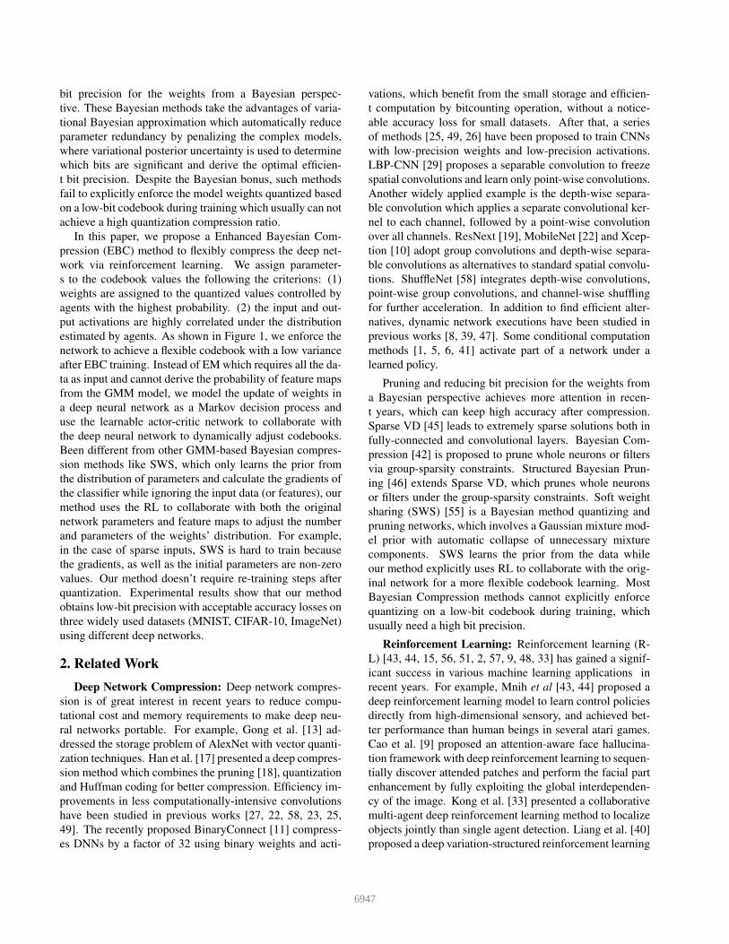
Figure 1. The main idea of the proposed Enhanced Bayesian Com-

pression (EBC) method. EBC aims to learn flexible codebooks in

each layer for an optimal network quantization. The original mod-

el weights in (a) have a new distribution as shown in (b) after our

EBC training, which can be directly quantized to the codebook

values with a restrained quantization error impact.

weight value, which may fail to determine the weights that

indeed contribute much to the overall computation. Net-

work quantization [18, 59, 28] has been proposed for the

reduction of the bit precision of weights, activations or

even gradients. For example, [18] employed a convention-

al quantization method for network quantization. However,

these methods suffer from accuracy losses because of the

quantization errors and rely on a highly computational re-

training after quantization. There are some other works in-

volving CNNs efficiency improvements, which have been

studied in previous works [27, 22, 58, 23]. For example,

[25, 49] are proposed using binary weights and activations,

which benefit from the small storage and efficient compu-

tation by bit-counting operation. Another popular variant is

depth-wise separable convolution [50], which applies a sep-

arate convolutional kernel to each channel, followed by a

point-wise convolution over all channels [10, 22, 58]. Most

of these methods focus on finding an efficient alternative for

standard spatial convolutions hence learning a compressed

network from scratch.

More recently, some compression methods [42, 55, 45,

46] have been proposed to prune the network and reduce

6946

bit precision for the weights from a Bayesian perspec-

tive. These Bayesian methods take the advantages of varia-

tional Bayesian approximation which automatically reduce

parameter redundancy by penalizing the complex models,

where variational posterior uncertainty is used to determine

which bits are significant and derive the optimal efficien-

t bit precision. Despite the Bayesian bonus, such methods

fail to explicitly enforce the model weights quantized based

on a low-bit codebook during training which usually can not

achieve a high quantization compression ratio.

In this paper, we propose a Enhanced Bayesian Com-

pression (EBC) method to flexibly compress the deep net-

work via reinforcement learning. We assign parameter-

s to the codebook values the following the criterions: (1)

weights are assigned to the quantized values controlled by

agents with the highest probability. (2) the input and out-

put activations are highly correlated under the distribution

estimated by agents. As shown in Figure 1, we enforce the

network to achieve a flexible codebook with a low variance

after EBC training. Instead of EM which requires all the da-

ta as input and cannot derive the probability of feature maps

from the GMM model, we model the update of weights in

a deep neural network as a Markov decision process and

use the learnable actor-critic network to collaborate with

the deep neural network to dynamically adjust codebooks.

Been different from other GMM-based Bayesian compres-

sion methods like SWS, which only learns the prior from

the distribution of parameters and calculate the gradients of

the classifier while ignoring the input data (or features), our

method uses the RL to collaborate with both the original

network parameters and feature maps to adjust the number

and parameters of the weights’ distribution. For example,

in the case of sparse inputs, SWS is hard to train because

the gradients, as well as the initial parameters are non-zero

values. Our method doesn’t require re-training steps after

quantization. Experimental results show that our method

obtains low-bit precision with acceptable accuracy losses on

three widely used datasets (MNIST, CIFAR-10, ImageNet)

using different deep networks.

2. Related Work

Deep Network Compression: Deep network compres-

sion is of great interest in recent years to reduce compu-

tational cost and memory requirements to make deep neu-

ral networks portable. For example, Gong et al. [13] ad-

dressed the storage problem of AlexNet with vector quanti-

zation techniques. Han et al. [17] presented a deep compres-

sion method which combines the pruning [18], quantization

and Huffman coding for better compression. Efficiency im-

provements in less computationally-intensive convolutions

have been studied in previous works [27, 22, 58, 23, 25,

49]. The recently proposed BinaryConnect [11] compress-

es DNNs by a factor of 32 using binary weights and acti-

vations, which benefit from the small storage and efficien-

t computation by bitcounting operation, without a notice-

able accuracy loss for small datasets. After that, a series

of methods [25, 49, 26] have been proposed to train CNNs

with low-precision weights and low-precision activations.

LBP-CNN [29] proposes a separable convolution to freeze

spatial convolutions and learn only point-wise convolutions.

Another widely applied example is the depth-wise separa-

ble convolution which applies a separate convolutional ker-

nel to each channel, followed by a point-wise convolution

over all channels. ResNext [19], MobileNet [22] and Xcep-

tion [10] adopt group convolutions and depth-wise separa-

ble convolutions as alternatives to standard spatial convolu-

tions. ShuffleNet [58] integrates depth-wise convolutions,

point-wise group convolutions, and channel-wise shuffling

for further acceleration. In addition to find efficient alter-

natives, dynamic network executions have been studied in

previous works [8, 39, 47]. Some conditional computation

methods [1, 5, 6, 41] activate part of a network under a

learned policy.

Pruning and reducing bit precision for the weights from

a Bayesian perspective achieves more attention in recen-

t years, which can keep high accuracy after compression.

Sparse VD [45] leads to extremely sparse solutions both in

fully-connected and convolutional layers. Bayesian Com-

pression [42] is proposed to prune whole neurons or filters

via group-sparsity constraints. Structured Bayesian Prun-

ing [46] extends Sparse VD, which prunes whole neurons

or filters under the group-sparsity constraints. Soft weight

sharing (SWS) [55] is a Bayesian method quantizing and

pruning networks, which involves a Gaussian mixture mod-

el prior with automatic collapse of unnecessary mixture

components. SWS learns the prior from the data while

our method explicitly uses RL to collaborate with the orig-

inal network for a more flexible codebook learning. Most

Bayesian Compression methods cannot explicitly enforce

quantizing on a low-bit codebook during training, which

usually need a high bit precision.

Reinforcement Learning: Reinforcement learning (R-

L) [43, 44, 15, 56, 51, 2, 57, 9, 48, 33] has gained a signif-

icant success in various machine learning applications in

recent years. For example, Mnih et al [43, 44] proposed a

deep reinforcement learning model to learn control policies

directly from high-dimensional sensory, and achieved bet-

ter performance than human beings in several atari games.

Cao et al. [9] proposed an attention-aware face hallucina-

tion framework with deep reinforcement learning to sequen-

tially discover attended patches and perform the facial part

enhancement by fully exploiting the global interdependen-

cy of the image. Kong et al. [33] presented a collaborative

multi-agent deep reinforcement learning method to localize

objects jointly than single agent detection. Liang et al. [40]

proposed a deep variation-structured reinforcement learning

6947

Actor Network Critic NetworkCritic Network

Convolutional network

......

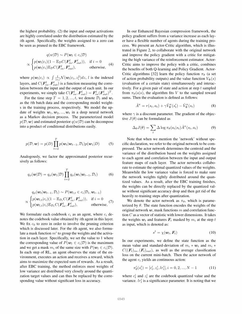
Figure 2. The framework of our proposed EBC approach, in which

the backbone CNN network and the Actor-Critic network collab-

orates to learns flexible codebooks. In each layer of the backbone

network, the actor network get state value and outputs an action

which is evaluated by the critic network for updating the code-

book.

framework to detect visual relationship and attributes with

a directed semantic action graph.

Recent works on searching models with reinforcemen-

t learning greatly improve the performance of neural net-

works. NAS [61] aims to search the transferable network

blocks whose performance surpasses many hand-crafted ar-

chitectures. N2N [3] integrated reinforcement learning in-

to channel selection. AMC [20] leveraged reinforcement

learning for deep compression policy, with higher compres-

sion ratio while preserving the accuracy, which outperforms

conventional rule-based compression policy. The concepts

of state, action, rewards and transitions in RL also motivate

us to leverage ideas from RL for Bayesian Compression.

Compared with previous works, EBC optimizes for both ac-

curacy and low-bit precision without any further re-training

steps or extra system computational overloads.

3. Approach

In this section, we first describe the deep network com-

pression framework from a Bayesian perspective. Then we

propose our Deep Reinforcement Learning for Bayesian

compression method. We map the problem of Bayesian

compression problem onto the policy optimization problem

via reinforcement learning. At last we introduce actor-critic

network to collaborate with original network and optimize

the EBC method for flexibly compression.

3.1. Bayesian Compression

Bayesian compression aims to prune deep networks and

reduce bit precision for the weights while keeping high

accuracy. The Bayesian methods [42, 55, 45, 46] search

for the optimal model structure and determine required bit-

precision per layer via uncertain posteriors over the param-

eters from a Bayesian perspective. In variational inference

the evidence lower bound (ELBO) LELBO = −(LE+LC)is maximized for an optimal trade-off between short de-

scription length of the data and the model. According to the

Minimum description length (MDL) principle, a model is

optimal if it can minimize the combined cost of the descrip-

tion of model complexity (LC) and the misfit between the

model and the data (LE). Bayesian methods investigate the

equivalence of variational inference and the MDL principle

based on the fundamental theorem in information theory.

Suppose we have a dataset D with N pairs of objects

(xn, yn)Nn=1. Let p(D|w) =

∏N

i=1 p(yi|xi,w) be a pa-

rameterized model that predicts outputs yi, given inputs xi

and parameters w about which we usually have some prior

knowledge p(w). In Bayesian learning, we are interested

in the posterior p(w|D) = p(D|w)p(w)/p(D), which is

intractable for many models. Variational Inference is ex-

ploited to approximate the posterior distribution p(w|D)by a parametric distribution qφ(w). Variational parameters

φ are optimized by minimizing the Kullback-Leibler diver-

gence, which denotes as DKL(qφ(w)||p(w|D)). Minimiz-

ing this KL divergence can be approximately performed by

maximizing the aforementioned ELBO, which is also called

”negative variational free energy” [31]:

L(φ) = LD(φ)−DKL(qφ(w)||p(w)) (1)

LD(φ) =

N∑

n=1

Eqφ(w)[log p(yn|xn, w)] (2)

where the variational lower bound in (1) and its gradients

can not be computed. Some existing methods [45, 42] use

the Reparameterization Trick to obtain an unbiased, differ-

entiable, minibatch-based Monte Carlo estimator of the ex-

pected log likelihood:

LSGV BD (φ) =

N

M

M∑

m=1

logp(ym|xm, f(φ, ǫm)) (3)

Unlike previous works which use the Reparameterization

Trick [7] to reduce variance of the stochastic ELBO gradient

estimator, we reformulate the intractable problem from a

reinforcement learning perspective. We provide a high level

connection between ELBO in Bayesian Compression and

the expected returns in reinforcement learning. We focus

on the computing gradients of expectations to further reduce

the variance of the unbiased reinforce estimator.

3.2. Enhanced Bayesian Compression via Deep Re-inforcement Learning

Let us revisit the parameterized model p(D,w) =p(D|w)p(w) and the estimated posterior q(w|D) from the

reinforcement point of view. We assign w to the codebook

value ci the following the criterions: (1) weights are as-

signed to the quantized values ck controlled by agent k with

6948

the highest probability. (2) the input and output activations

are highly correlated under the distribution estimated by the

ith agent. Specifically, the weights assigned to a zero can

be seen as pruned in the EBC framework.

q(w|D) ∼ P (wl ∈ ci|D)

∝

{

p(wl|ci)(1− EDC(F lin,F

lout)), if i = 0

p(wl|ci)EDC(F lin,F

lout), otherwise,

(4)

where p(wl|ci) ∝∫

1|zi|N (wl|ci, z

2i )dz, l is the indexed

layers, and C(F lin,F

lout) is a function measuring the corre-

lation between the input and the output of each unit. In our

experiments, we simply take C(F lin,F

lout) = F l

in(Flout)

T .

For the time step T = 1, 2, ..., t, we denote Dt and wt

as the tth batch data and the corresponding model weight-

s in the training process, respectively. We model the up-

date of weights w1,w2, ...,wt in a deep neural network

as a Markov decision process. The parameterized model

p(D,w) and estimated posterior q(w|D) can be decompose

into a product of conditional distributions easily.

p(D,w) = p(D)

T∏

t=2

p(wt|wt−1,Dt)p(w1|D) (5)

Analogously, we factor the approximated posterior recur-

sively as follows:

qφ(w|D) = qφ(w1|D)

T∏

t=2

qφ(wt|wt−1,Dt) (6)

qφ(wt|wt−1,Dt) ∼ P (wl,t ∈ ci|Dt,wt−1)

∝

{

p(wl,t|ci)(1− EDtC(F l

in,Flout)), if i = 0

p(wl,t|ci)EDtC(F l

in,Flout), otherwise,

(7)

We formulate each codebook ci as an agent, where ci de-

notes the codebook value obtained by ith agent in this layer.

We fix c0 to zero in order to involve the pruning criterion

which is discussed later. For the ith agent, we also formu-

late a mask function mi to group the weights and the activa-

tion in each layer. Specifically, we set the value to 1 where

the corresponding value of P (wl ∈ ci|D) is the maximum

and we get a mask mi of the same size with P (wl ∈ ci|D).In each step of RL, an agent observes the state of the en-

vironment, executes an action and receives a reward, which

aims to maximize the expected sum of rewards. As a result,

after EBC training, the method enforces most weights of

low variance are distributed very closely around the quanti-

zation target values and can thus be replaced by the corre-

sponding value without significant loss in accuracy.

In our Enhanced Bayesian compression framework, the

policy gradient suffers from a variance increase as each lay-

er have a flexible number of agents during the training pro-

cess. We present an Actor-Critic algorithm, which is illus-

trated in Figure 2, to collaborate with the original network

and improve the policy gradient with a critic for mitigat-

ing the high variance of the reinforcement estimator. Actor-

Critic aims to improve the policy with a critic, combines

the benefits of both Q-learning and Policy Gradient. Actor-

Critic algorithms [32] learn the policy function πθ (a set

of action probability outputs) and the value function VΦ(s)(evaluation of a certain state) simultaneously and interac-

tively. For a given pair of state and action at step t sampled

from πθ(a|s), the algorithm fits V to the sampled reward

sums. Then the evaluation is defined as follows:

Aπ = r(st, at) + γV πΦ (s′t)− V π

Φ (st) (8)

where γ is a discount parameter. The gradient of the objec-

tive J(θ) can be formulated as

∆θJ(θ) =∑

t

∆ log πθ(at|st)Aπ(st, at) (9)

Note that when we mention the ’network’ without spe-

cific declaration, we refer to the original network to be com-

pressed. The actor network determines the centroid and the

variance of the distribution based on the weights assigned

to each agent and correlation between the input and output

feature maps of each layer. The actor networks collabo-

rate to estimate the optimal quantized values of the weights.

Meanwhile the low variance value is forced to make sure

the network weights tightly distributed around the quan-

tized values. As a result, after the EBC training finishes,

the weights can be directly replaced by the quantized val-

ue without significant accuracy drop and then get rid of the

heavily re-training steps after quantization.

We denote the actor network as πθ, which is parame-

terized by θ. The state function encodes the weights of the

original network w, mask functions m and correlation func-

tion C as a vector of statistic with lower dimensions. It takes

the weights wt and features Ft masked by mi at the step tas input, which is denoted as:

st = χ(wt,Ft) (10)

In our experiments, we define the state function as the

mean value and standard-deviation of mi ∗ wt and mi ∗C((Ft)in, (Ft)out), as well as the average classification

loss on the current mini-batch. Then the actor network of

the agent vi yields an continuous action:

πiθ(s

ti) = [cit, z

it, lr

it], i = 0, 2, ..., N − 1 (11)

where cit and zit are the codebook quantized value and the

variance. lrit is a significance parameter. It is noting that we

6949

always keep c0t to be zero by masking it since the weights

assigned to c0t are pruned. In addition to the adaptive code-

book values, our EBC framework allows flexible number of

codebooks by adjusting the number of agents. To achieve

this goal, we define two discrete actions {delete node,add

node} for the agent i (i 6= 0) at the end of each training

epoch. Using a threshold on αl as a criterion in lth lay-

er is equivalent to delete the agent whose ratio of assigned

weights is low:

||m(i)||1

nl−1nl≤ αl (12)

To be precise, (12) specifies the sparsity of the weights as-

signed to an agent. Also, for lth layer we use a threshold on

βl as a criterion to split one agent with large into two:

max(z(i))∑

i z(i)

≥ βl (13)

In our experiments, αl and βl are set to keep the same val-

ue respectively across the layers. Then we reinitialize the

codebook value ci as ci±zi√2

To be precise, (13) forces the

variance of the weights assigned to an agent be constrained

below a threshold. where zi denotes the variance. In our E-

BC framework, the long term reward of the state-action pair

is related to the accumulative decrement of negative accura-

cy drop (−(acct− acct+1) = ∆acc) and the KL divergency

approximation. We define the immediate reward at step as:

rt =∑

i

lrip(wt) log(p(wt|wt−1,Dt−1)

q(wt|wt−1,Dt)+ ∆acc (14)

The accumulative value Rt′

π =∑T

t=t′ γt−t′rt +

γT−t′ log p(D|w1). The critic network uses the function

QΦ which is parameterized by Φ to approximate the Q val-

ue function. For each agent, the critic network only outputs

one value at the final layer to evaluate the action.

Recall the third output lri of the actor network, this pa-

rameter is in fact a learning multiplier which denotes the

significance of each layer as well as each peak. This is mo-

tivated by the fact that the impact of quantization errors on

the accuracy varies across layers and peaks within each lay-

er. our proposed EBC can be optimized for quantizing all

layers of a network together for flexible optimal codebook-

s by exploiting the learning multiplier in (14). For deep

neural networks, this is feasible since layer-by-layer quan-

tization bit precise optimization requires exponential time

complexity with respect to the number of layers. To train

the Actor-Critic network, we first formulate the optimiza-

tion problem with respect to the critic network Φ by mini-

mizing the Temporal difference (TD) learning error as:

minΦ

L(Φ) = Es,a(QΦ(st, at)− rt − γQΦ(s

t+1, at+1)2

(15)

Algorithm 1 : EBC

Input: Training steps T; training set X; state function χ;

discount factor γ;

Output: Model weights w, policy parameters θ of the

actor network and the value parameters Φ of the critic

network.

Initialize w, θ, Φ// update strategy for ith agent of layer lfor t = 1 to T do

Sample a batch data xp ∈ XEncode the state vector: sti = χ(wt,F

pt )

// actor network outputs an action

Update the codebook value: cti = πθ(sti)

Update the model parameters w by back-propagation.

// update critic network

Compute reward rt using (14)

Compute (15) and update Φ using (16)

// update actor network

Sample a batch data xq ∈ X and q 6= pEncode the state vector: st+1

i = χ(wt,Fqt )

Compute at+1j = πθ(s

t+1j )

Update θ using (17)

end for

Delete or Add an agent using (12) and (13)

We update the parameters of the network Φ as follows:

Φ = Φ− µΦ∂L(Φ)

∂Φ(16)

We update the parameters θ to output the action with the

largest Q value, which is formulated as:

θ = θ − µθ

∂QΦ(st+1, at+1)

∂a

∂πθ(st+1)

∂θ|a=πθ(s) (17)

During the EBC training in each epoch, we update the

codebook values and the significance parameters according

to the Actor-Critic network while keeping the length of each

codebook unchanged. After training of one epoch is fin-

ished, the codebook length is updated by adding or deleting

the agents in each layer.

Algorithm 1 summarizes the learning procedure of our

EBC.

4. Experiments

We conducted experiments on three different datasets in-

cluding MNIST [36], CIFAR-10 [34] and ImageNet [12]

to show the effectiveness of our method. For MNIST, we

applied our EBC to LeNet [37] and compared the results

obtained by our EBC with recent state-of-the-art network

compression methods. For CIFAR-10, we applied our EBC

6950

to VGG-16 [52] and ResNet-18 [19] and reported the result-

s. For ImageNet, we applied our EBC to ResNet-18 [19]

and reported the results.

4.1. Implementation Details

We trained EBC in an iterative manner, where the o-

riginal network and the Actor-Critic network were trained

collaboratively. The Actor-Critic algorithm are operated on

mini-batches, each step is a mini batch in our experiments.

We define the state function χ as mean value and standard-

deviation of mi ∗wt and mi ∗ C((Ft)in, (Ft)out), as well

as the average classification loss on the current mini-batch,

which encodes the input as a state vector with 5 elements.

The thresholds α and β in (12) and (13) are set to 1e-3 and

0.3, respectively. The actor network in our experiment is

a two-layer long short-term memory (LSTM) [21] network

with 20 units in each layer. We specified the critic network

as a simple neural network with one hidden layer and 10

hidden units. We use the Adam optimizer [30] with a learn-

ing rate of 0.001 and a discount of γ (set as 0.95) to train

the Actor-Critic network. We implemented our methods in

Python using Pytorch library and conducted all the experi-

ments on GeForce GTX 1080 Ti GPU with 11GB VRAM.

During training, EBC gets rid of the warm-up [54] strate-

gy for the KL divergency term used by existing Bayesian

compression methods, since the actor network output lritautomatically determines the significance parameter which

helps in avoiding bad local optima. At the end of the net-

work train epochs, we obtain codebooks of different length-

s for each layer via Actor-Critic network. We adopted a

quantization step by assigning the weights to their closes-

t codebook values and then remove Actor-Critic network.

Having completed the training procedure of EBC, we em-

ploy the compressed network for inference directly, where

the Actor-Critic network s not required.

4.2. Results on MNIST

MNIST [36] is a database of handwritten digits which

is widely used to experimentally evaluate machine learn-

ing methods. We conducted the image preprocessing by

subtracting the mean value and dividing by the standard-

deviation over the training set. Following the same set-

tings with [42], we demonstrate our method on two mod-

els: LeNet-300-100 [37] and LeNet-5. LeNet-300-100 is a

feedforward neural network with three fully connected lay-

ers. LeNet-5 is a conventional CNN model which consists

of 4 learnable layers, including 2 convolutional layers and 2

fully connected layers. For both LeNet-300-100 and LeNet-

5, we train the full precision model using the standard SGD

method for 20 epochs to obtain the original top-1 test error

1.6% and 0.9%.

The proposed EBC method can be both applied to fine-

tuning a pre-trained networks and training the networks

Table 1. Results on the dataset using LeNet-300-100, showing the

top-1 test error, the percentage of non-pruned weights and the bit-

precision per parameter. Original is the uncompressed pre-trained

model. DC corresponds to Deep Compression method [17], DNS

to the method of [16], SWS to the Soft-Weight Sharing of [55],

Sparse VD to the variational dropout method at [45], BC refers to

BC-GHS version in Bayesian Compression in [42], BNN refers to

Binarized Neural networks in [25]

Method Test error(%)|w 6=0||w| (%) Bits

Original 1.6 100 32

DC 1.6 8.0 8-9

DNS 2.0 1.8 −SWS 1.9 4.3 3

Sparse VD 1.8 2.2 8-14

BC 1.8 0.6 10-13

BNN 2.4 − 1

EBC 1.8 1.6 2

Table 2. Results on the dataset using LeNet-5, showing the top-

1 test error, the percentage of non-pruned weights and the bit-

precision per parameter. Original is the uncompressed pre-trained

model. DC corresponds to Deep Compression method [17], DNS

to the method of [16], SWS to the Soft-Weight Sharing of [55],

Sparse VD to the variational dropout method at [45], BC refers to

BC-GHS version in Bayesian Compression in [42], BNN refers to

Binarized Neural networks in [25]

Method Test error(%)|w 6=0||w| (%) Bits

Original 0.9 100 32

DC 0.7 8.0 10-13

DNS 0.9 0.9 −SWS 1.0 3 3

Sparse VD 1.0 0.7 8-13

BC 1.0 0.6 10-14

BNN 1.2 − 1

EBC 1.0 0.7 2

from scratch. On MNIST, we trained both LeNet-300-100

and LeNet-5 using EBC from scratch, where all the weights

are randomly initialized. The batch size is 128 and the total

epoch is 200. Figure 3 shows the comparison of test loss

and accuracy between the original LeNet-5 and the com-

pressed LeNet-5 during the first 100 epochs. We denote the

original model here as the model trained by our EBC with-

out quantized to the codebooks. We find that during the first

few epochs, the accuracy of compressed models drops a lot

after quantized the original model. As the epochs increase,

the original model converges collaborated with the Actor-

Critic Network and weights of each layer are enforced to

6951

0 20 40 60 80 100

epoch

0

0.5

1

loss v

alu

e

test loss(original model)

test loss(compressed model)

(a) comparison of test loss

0 20 40 60 80 10050

60

70

80

90

100

test accuracy

test accuracy(original model)

test accurary(compressed model)

(b) comparison of test accuracy

Figure 3. Comparison of test loss and accuracy between the o-

riginal LeNet-5 and the compressed LeNet-5 during the first 100

epochs on MNIST dataset.

0 50 100 150 200

epoch

0

0.5

1

1.5

2

loss v

alu

e

test loss(original model)

test loss(compressed model)

(a) comparision of test loss

0 50 100 150 200

epoch

50

60

70

80

90

100

test accuracy

test accuracy(original model)

test accurary(compressed model)

(b) comparision of test accuracy

Figure 4. Comparison of test loss and accuracy between the o-

riginal VGG-16 and the compressed VGG-16 during the first 200

epochs on CIFAR-10 dataset.

distributed tightly around the quantized values given by the

actor network. Having completed the EBC training, we ob-

tain a network which can be directly quantized (quantized

to 0 means pruning) without a noticeable accuracy drop and

the quantized model can be directly applied to the classifica-

tion task in no need of finetuning. Table 1 and Table 2 show

the results compared with the state-of-the-art compression

methods. We denote the original model in the tables as the

pretrained LeNet model in the table. Our method achieves a

very low bit precision with a small accuracy loss (0.2% and

0.1%). The codebooks length determined by agents of each

layer of both LeNet-300-100 and LeNet-5 are 3 (2bit) for all

layers after convergency of the EBC. We also compared our

EBC with BNN which extremely quantizes the weights to 1

bit on LeNet-300-100 and LeNet-5 trained by Theano [4].

The result shows that BNN suffers from a higher accuracy

drop than ours because of a fixed quantization value.

4.3. Results on CIFAR-10

We demonstrate our method with VGG-16 [52] and

ResNet-18 [19] on the CIFAR-10 dataset [34]. VGG-16 has

13 convolutional layers and more parameters and ResNet-

18 is a 18 layer version of ResNet which has batch normal-

ization layers and shortcut connections. We trained the full

precision model using the standard SGD method for 200 e-

pochs to obtain the original top-1 test error 7.1% and 6.8%.

To help the EBC training converge faster, we pretrained the

Table 3. Results on the dataset CIFAR-10 using VGG-16, show-

ing the top-1 test error, the percentage of non-pruned weights and

the bit-precision per parameter. Original is the uncompressed pre-

trained model. BC refers to BC-GNJ version in Bayesian Com-

pression in [42], BNN refers to Binarized Neural networks in [25]

Method Test error(%)|w 6=0||w| (%) Bits

Original 8.4 100 32

BC 8.6 6.7 5-11

BNN 10.2 − 1

EBC 8.8 8.0 3-4

Table 4. Results on the dataset CIFAR-10 using and ResNet-18,

showing the top-1 test error, the percentage of non-pruned weights

and the bit-precision per parameter. Original is the uncompressed

pre-trained model. BC refers to BC-GNJ version in Bayesian

Compression in [42], BNN refers to Binarized Neural networks

in [25]

Method Test error(%)|w 6=0||w| (%) Bits

Original 6.8 100 32

BC 7.5 4.4 5-17

BNN 10.8 − 1

SWS 8.3 7.3 3

EBC 7.2 3.5 3-4

two models for 100 epochs using Adam and obtain top-

1 test error 15.6% and 14.7% on CIFAR-10, respectively.

Figure 4 shows the comparison of test loss and accuracy

between the original VGG-16 and the compressed VGG-16

keep consistent even at the first few epochs because of the

usage of pretrained model accelerates the convergency. Ta-

ble 3 and Table 4 shows the results compared with Bayesian

Compression, where the required bit-precision per layer is

determined via posterior uncertainty without explicitly en-

forcing to learn codebooks for quantization. Our method

achieves the lower bit precision than Bayesian Compression

with a small accuracy loss (0.4% for VGG-16 and 1.4% for

ResNet-18). The codebooks length determined by agents of

each layer of VGG-16 ranges from 5 to 11 (3-4 bits) while

ResNet-18 ranges from 7-13 (3-4 bit).

4.4. Results on ImageNet

ImageNet is a large dataset covering 1,000 categories

for visual recognition. It contains over 1.2M images in the

training set and 50K images in the validation set. For this

dataset, we report both Top-1 and Top-5 validation accu-

racy. On this dataset, we compare our EBC with the re-

cent proposed low-bits methods: BWN [49], TWN [38],

TTQ [60] to demonstrate the effectiveness of flexible code-

books. We cannot directly compare the related Bayesian

methods since the authors do not report results on Ima-

6952

-100 -50 0 50 100 -2000 -1000 0 1000 2000 -400 -200 0 200 400

(a) Distribution of pretrained model.

-5 0 5

×10 -5

-1 -0.5 0 0.5 1

×10 -5-1 -0.5 0 0.5 1

(b) Distribution of EBC trained model at epoch 100.

-2 -1 0 1 2

×10 -5

-1 -0.5 0 0.5 1

×10 -5-1 -0.5 0 0.5 1

(c) Distribution of EBC trained model at epoch 200.

Figure 5. Visualization of the weights distribution in the conv3,

conv5 and conv7 layer (from left to right) of pretrained VGG-16

on CIFAR-10 at 200th epoch (from top to bottom), EBC trained

model at 100th epoch and EBC trained model at 200th epoch.

EBC model Original model

conv3 conv3 conv5 conv7conv5 conv7

Figure 6. Visualization of the original images, the feature maps of

the conv3, conv5 and conv7 layers of EBC models and original

models (VGG-16), respectively. The presented feature maps are

averaged over the channels.

geNet. We trained the full precision model using the stan-

dard SGD method for 100 epochs to obtain the original top-

1 and top-5 validation error 31.6% and 11.3%. The results

are summarized in Table 5. We see that our EBC trained

model with flexible bit-precision performs better than BNN-

like methods on ImageNet with memory only exceeding a

little.

Table 5. Results on the dataset ImageNet using ResNet-18, show-

ing the top-1 and top-5 validation error, the percentage of non-

pruned weights and the bit-precision per parameter. Original is

the uncompressed pre-trained model.

Method Val error(Top-1/Top-5)(%) Bits

Original 31.6/11.3 32

BWN 39.2/17.0 1

TWN 34.5/14.0 2

TTQ 34.1/13.8 2

SWS(I) 34.2/13.5 3

EBC 31.8/11.4 3-4

4.5. Visualization

Figure 5 shows the visualization of the weights distri-

bution in the conv3 layer, conv5 layer and conv7 layer of

pretrained VGG-16 at 200th epoch, EBC trained model at

100th epoch and EBC trained model at 200th epoch. We

see that the weights distribution of each peak is more tight

as the EBC training epoch increases.

We have also visualized the functionality of our EBC

models by calculating average feature maps produced by

convolution layers since the spatial feature maps of CNNs

shows where the network focuses hence influence the final

classification results of the given images. The results are

shown in Figure 6. From the figure, we see that the feature

maps of the compressed layers are very close to that of the

original ones, even with a large reduction on model weights.

5. Conclusion

In this paper, we have proposed a enhanced reinforce-

ment learning method to flexibly compress the deep net-

work via reinforcement learning. An Actor-Critic network,

which collaborates with the original network, is exploited

to learn flexible codebooks in each layer for an optimal net-

work quantization. With our EBC method, the model does-

n’t require re-training after the quantization. Experimental

results on three datasets have been presented to demonstrate

the effectiveness of our method.

Acknowledgements

This work was supported in part by the National Key

Research and Development Program of China under Grant

2016YFB1001001, in part by the National Natural Sci-

ence Foundation of China under Grant 61672306, Grant

U1713214, Grant 61572271, and in part by the Shenzhen

Fundamental Research Fund (Subject Arrangement) under

Grant JCYJ20170412170602564.

6953

References

[1] A. Almahairi, N. Ballas, T. Cooijmans, Y. Zheng,

H. Larochelle, and A. C. Courville. Dynamic capacity net-

works. In ICML, pages 2549–2558, 2016.

[2] H. B. Ammar, E. Eaton, P. Ruvolo, and M. Taylor. Online

multi-task learning for policy gradient methods. In ICML,

pages 1206–1214, 2014.

[3] A. Ashok, N. Rhinehart, F. Beainy, and K. M. Kitani. N2N

learning: Network to network compression via policy gradi-

ent reinforcement learning. ICLR, abs/1709.06030, 2017.

[4] F. Bastien, P. Lamblin, R. Pascanu, J. Bergstra, I. Good-

fellow, A. Bergeron, N. Bouchard, D. Warde-Farley, and

Y. Bengio. Theano: new features and speed improvements.

arXiv preprint arXiv:1211.5590, 2012.

[5] E. Bengio, P. Bacon, J. Pineau, and D. Precup. Conditional

computation in neural networks for faster models. CoRR,

abs/1511.06297, 2015.

[6] Y. Bengio, N. Leonard, and A. C. Courville. Estimating or

propagating gradients through stochastic neurons for condi-

tional computation. CoRR, abs/1308.3432, 2013.

[7] A. Blum, N. Haghtalab, and A. D. Procaccia. Variation-

al dropout and the local reparameterization trick. In NIPS,

pages 2575–2583, 2015.

[8] T. Bolukbasi, J. Wang, O. Dekel, and V. Saligrama. Adap-

tive neural networks for fast test-time prediction. CoRR, ab-

s/1702.07811, 2017.

[9] Q. Cao, L. Lin, Y. Shi, X. Liang, and G. Li. Attention-aware

face hallucination via deep reinforcement learning. In CVPR,

pages 690–698, 2017.

[10] F. Chollet. Xception: Deep learning with depthwise separa-

ble convolutions. In CVPR, pages 1800–1807, 2017.

[11] M. Courbariaux, Y. Bengio, and J. David. Binaryconnect:

Training deep neural networks with binary weights during

propagations. In NIPS, pages 3123–3131, 2015.

[12] J. Deng, W. Dong, R. Socher, L. Li, K. Li, and F. Li. Ima-

genet: A large-scale hierarchical image database. In CVPR,

pages 248–255, 2009.

[13] Y. Gong, L. Liu, M. Yang, and L. D. Bourdev. Compress-

ing deep convolutional networks using vector quantization.

CoRR, abs/1412.6115, 2014.

[14] A. Graves and N. Jaitly. Towards end-to-end speech recogni-

tion with recurrent neural networks. In ICML, pages 1764–

1772, 2014.

[15] S. Gu, T. Lillicrap, I. Sutskever, and S. Levine. Continuous

deep q-learning with model-based acceleration. In ICML,

pages 2829–2838, 2016.

[16] Y. Guo, A. Yao, and Y. Chen. Dynamic network surgery for

efficient dnns. In NIPS, pages 1379–1387, 2016.

[17] S. Han, H. Mao, and W. J. Dally. Deep compression: Com-

pressing deep neural network with pruning, trained quanti-

zation and huffman coding. CoRR, abs/1510.00149, 2015.

[18] S. Han, J. Pool, J. Tran, and W. J. Dally. Learning both

weights and connections for efficient neural networks. CoR-

R, abs/1506.02626, 2015.

[19] K. He, X. Zhang, S. Ren, and J. Sun. Deep residual learning

for image recognition. In CVPR, pages 770–778, 2016.

[20] Y. He, J. Lin, Z. Liu, H. Wang, L. Li, and S. Han. AMC:

automl for model compression and acceleration on mobile

devices. In ECCV, pages 815–832, 2018.

[21] S. Hochreiter and J. Schmidhuber. Long short-term memory.

Neural computation, 9(8):1735–1780, 1997.

[22] A. G. Howard, M. Zhu, B. Chen, D. Kalenichenko, W. Wang,

T. Weyand, M. Andreetto, and H. Adam. Mobilenets: Effi-

cient convolutional neural networks for mobile vision appli-

cations. CoRR, abs/1704.04861, 2017.

[23] G. Huang, S. Liu, L. van der Maaten, and K. Q. Weinberg-

er. Condensenet: An efficient densenet using learned group

convolutions. CoRR, abs/1711.09224, 2017.

[24] G. Huang, Z. Liu, L. van der Maaten, and K. Q. Weinberger.

Densely connected convolutional networks. In CVPR, pages

2261–2269, 2017.

[25] I. Hubara, M. Courbariaux, D. Soudry, R. El-Yaniv, and

Y. Bengio. Binarized neural networks. In NIPS, pages 4107–

4115, 2016.

[26] I. Hubara, M. Courbariaux, D. Soudry, R. El-Yaniv, and

Y. Bengio. Quantized neural networks: Training neural net-

works with low precision weights and activations. CoRR,

abs/1609.07061, 2016.

[27] F. N. Iandola, M. W. Moskewicz, K. Ashraf, S. Han, W. J.

Dally, and K. Keutzer. Squeezenet: Alexnet-level accuracy

with 50x fewer parameters and <1mb model size. CoRR,

abs/1602.07360, 2016.

[28] B. Jacob, S. Kligys, B. Chen, M. Zhu, M. Tang, A. G.

Howard, H. Adam, and D. Kalenichenko. Quantization and

training of neural networks for efficient integer-arithmetic-

only inference. CoRR, abs/1712.05877, 2017.

[29] F. Juefei-Xu, V. N. Boddeti, and M. Savvides. Local binary

convolutional neural networks. In CVPR, pages 4284–4293,

2017.

[30] D. P. Kingma and J. Ba. Adam: A method for stochastic

optimization. CoRR, abs/1412.6980, 2014.

[31] D. P. Kingma and M. Welling. Auto-encoding variational

bayes. CoRR, abs/1312.6114, 2013.

[32] V. R. Konda and J. N. Tsitsiklis. Actor-critic algorithms. In

NIPS, pages 1008–1014, 1999.

[33] X. Kong, B. Xin, Y. Wang, and G. Hua. Collaborative deep

reinforcement learning for joint object search. In CVPR,

2017.

[34] A. Krizhevsky and G. Hinton. Learning multiple layers of

features from tiny images. 2009.

[35] A. Krizhevsky, I. Sutskever, and G. E. Hinton. Imagenet

classification with deep convolutional neural networks. In

NIPS, pages 1097–1105, 2012.

[36] Y. LeCun. The mnist database of handwritten digits.

http://yann. lecun. com/exdb/mnist/, 1998.

[37] Y. LeCun, L. Bottou, Y. Bengio, and P. Haffner. Gradient-

based learning applied to document recognition. Proceed-

ings of the IEEE, 86(11):2278–2324, 1998.

[38] F. Li and B. Liu. Ternary weight networks. CoRR, ab-

s/1605.04711, 2016.

[39] H. Li, Z. Lin, X. Shen, J. Brandt, and G. Hua. A convolu-

tional neural network cascade for face detection. In CVPR,

pages 5325–5334, 2015.

6954

[40] X. Liang, L. Lee, and E. P. Xing. Deep variation-structured

reinforcement learning for visual relationship and attribute

detection. In CVPR, pages 848–857, 2017.

[41] L. Liu and J. Deng. Dynamic deep neural networks: Opti-

mizing accuracy-efficiency trade-offs by selective execution.

CoRR, abs/1701.00299, 2017.

[42] C. Louizos, K. Ullrich, and M. Welling. Bayesian compres-

sion for deep learning. In NIPS, pages 3290–3300, 2017.

[43] V. Mnih, K. Kavukcuoglu, D. Silver, A. Graves,

I. Antonoglou, D. Wierstra, and M. Riedmiller. Playing

atari with deep reinforcement learning. arXiv preprint arX-

iv:1312.5602, 2013.

[44] V. Mnih, K. Kavukcuoglu, D. Silver, A. A. Rusu, J. Veness,

M. G. Bellemare, A. Graves, M. Riedmiller, A. K. Fidjeland,

G. Ostrovski, et al. Human-level control through deep rein-

forcement learning. Nature, 518(7540):529–533, 2015.

[45] D. Molchanov, A. Ashukha, and D. P. Vetrov. Variation-

al dropout sparsifies deep neural networks. In ICML, pages

2498–2507, 2017.

[46] K. Neklyudov, D. Molchanov, A. Ashukha, and D. P. Vetro-

v. Structured bayesian pruning via log-normal multiplicative

noise. In NIPS, pages 6778–6787, 2017.

[47] A. Odena, D. Lawson, and C. Olah. Changing model be-

havior at test-time using reinforcement learning. CoRR, ab-

s/1702.07780, 2017.

[48] Y. Rao, J. Lu, and J. Zhou. Attention-aware deep reinforce-

ment learning for video face recognition. In ICCV, pages

3931–3940, 2017.

[49] M. Rastegari, V. Ordonez, J. Redmon, and A. Farhadi. Xnor-

net: Imagenet classification using binary convolutional neu-

ral networks. In ECCV, pages 525–542, 2016.

[50] L. Sifre and P. Mallat. Rigid-motion scattering for image

classification. PhD thesis, Citeseer, 2014.

[51] D. Silver, G. Lever, N. Heess, T. Degris, D. Wierstra, and

M. Riedmiller. Deterministic policy gradient algorithms. In

ICML, pages 387–395, 2014.

[52] K. Simonyan and A. Zisserman. Very deep convolution-

al networks for large-scale image recognition. CoRR, ab-

s/1409.1556, 2014.

[53] R. Socher, C. C. Lin, A. Y. Ng, and C. D. Manning. Pars-

ing natural scenes and natural language with recursive neural

networks. In ICML, pages 129–136, 2011.

[54] C. K. Sønderby, T. Raiko, L. Maaløe, S. K. Sønderby, and

O. Winther. Ladder variational autoencoders. In NIPS, pages

3738–3746, 2016.

[55] K. Ullrich, E. Meeds, and M. Welling. Soft weight-sharing

for neural network compression. ICLR, 2017.

[56] H. Van Hasselt, A. Guez, and D. Silver. Deep reinforcement

learning with double q-learning. In AAAI, pages 2094–2100,

2016.

[57] L. Yu, W. Zhang, J. Wang, and Y. Yu. Seqgan: Sequence

generative adversarial nets with policy gradient. In AAAI,

pages 2852–2858, 2017.

[58] X. Zhang, X. Zhou, M. Lin, and J. Sun. Shufflenet: An

extremely efficient convolutional neural network for mobile

devices. CoRR, abs/1707.01083, 2017.

[59] A. Zhou, A. Yao, Y. Guo, L. Xu, and Y. Chen. Incremen-

tal network quantization: Towards lossless cnns with low-

precision weights. CoRR, abs/1702.03044, 2017.

[60] C. Zhu, S. Han, H. Mao, and W. J. Dally. Trained ternary

quantization. CoRR, abs/1612.01064, 2016.

[61] B. Zoph, V. Vasudevan, J. Shlens, and Q. V. Le. Learn-

ing transferable architectures for scalable image recognition.

CoRR, abs/1707.07012, 2017.

6955