Embed Size (px)
Citation preview

AUTOMATIC STROKE LESION SEGMENTATION WITH
LIMITED MODALITIES
by
Craig W. Fraser
B. S. Electrical Engineering, University of Pittsburgh, 2012
Submitted to the Graduate Faculty of
the Swanson School of Engineering in partial fulfillment
of the requirements for the degree of
Master of Science
University of Pittsburgh
2016

UNIVERSITY OF PITTSBURGH
SWANSON SCHOOL OF ENGINEERING
This thesis was presented
by
Craig W. Fraser
It was defended on
November 29, 2016
and approved by
Steven P. Jacobs, Ph.D., Assistant Professor, Department of Electrical and Computer Engineering
Murat Akcakaya, Ph.D., Assistant Professor, Department of Electrical and Computer Engineering
Ching-Chung Li, Ph.D., Professor, Department of Electrical and Computer Engineering
Thesis Advisor: Steven P. Jacobs, Ph.D., Assistant Professor, Department of Electrical and
Computer Engineering
ii

Copyright c© by Craig W. Fraser
2016
iii

AUTOMATIC STROKE LESION SEGMENTATION WITH LIMITED MODALITIES
Craig W. Fraser, M.S.
University of Pittsburgh, 2016
MRI Brain image segmentation is a valuable tool in the diagnosis and treatment of many different
types of brain damage. There is a strong push for development of computerized segmentation
algorithms that can automate this process because segmentation by hand requires a great deal of
effort by a highly skilled professional. While hand segmentation is currently considered the gold
standard, it is not without flaws; for example, segmentation by two different people can provide
slightly different results, and segmentation by hand is labor intensive. Due to these flaws, It is
desirable to make this process more consistent and more efficient through computer automation.
This project investigates four promising approaches for the automatic segmentation of brain
MRIs containing stroke lesions found in recent literature. Two of these algorithms are designed to
use multiple modalities of the same patient during segmentation, while the other two are designed
to handle one specific modality. The robustness of each to limited, or different, image sequences
than they were originally designed for will be tested by applying each to two datasets that contain
24 and 36 patients with chronic stroke lesions.
These tests concluded that performance for the multi modal algorithms does tend to decrease
as input modalities are removed, however it also revealed that FLAIR imaging in particular seems
to be especially valuable for segmenting stroke lesions. In both multi-modal algorithms while there
was an overall drop in Dice scores, any testing that included FLAIR images performed significantly
better than any other tests. The single channel algorithms had difficulty segmenting any modalities
different from the specific one that they were designed for, and were generally unable to detect
very small lesions.
iv

TABLE OF CONTENTS
1.0 INTRODUCTION . . . . . . . . . . . . . . . . . . . . . . . . . . . . . . . . . . . . 1
1.1 PROBLEM STATEMENT . . . . . . . . . . . . . . . . . . . . . . . . . . . . . . 1
1.2 SCOPE AND OBJECTIVES . . . . . . . . . . . . . . . . . . . . . . . . . . . . . 2
1.3 ORGANIZATION OF THESIS . . . . . . . . . . . . . . . . . . . . . . . . . . . 2
2.0 BACKGROUND . . . . . . . . . . . . . . . . . . . . . . . . . . . . . . . . . . . . . 4
3.0 LITERATURE REVIEW . . . . . . . . . . . . . . . . . . . . . . . . . . . . . . . . 7
3.1 GENERATIVE MODEL WITH BIOLOGICAL CONSTRAINTS . . . . . . . . . 7
3.2 SEGMENTATION USING CONVOLUTIONAL NEURAL NETWORKS . . . . 9
3.3 DISCRIMINATING SEGMENTS BY HISTOGRAM MAXIMA . . . . . . . . . 10
3.4 SEGMENTATION BY NEIGHBORHOOD DATA ANALYSIS . . . . . . . . . . 11
3.5 METRICS FOR EVALUATING SEGMENTATIONS . . . . . . . . . . . . . . . . 12
4.0 METHODS . . . . . . . . . . . . . . . . . . . . . . . . . . . . . . . . . . . . . . . . 18
4.1 INPUT DATA . . . . . . . . . . . . . . . . . . . . . . . . . . . . . . . . . . . . . 18
4.2 DEEPMEDIC . . . . . . . . . . . . . . . . . . . . . . . . . . . . . . . . . . . . . 19
4.2.1 THEORY . . . . . . . . . . . . . . . . . . . . . . . . . . . . . . . . . . . . 19
4.2.2 IMPLEMENTATION . . . . . . . . . . . . . . . . . . . . . . . . . . . . . 21
4.3 GENERATIVE MODEL . . . . . . . . . . . . . . . . . . . . . . . . . . . . . . . 23
4.3.1 THEORY . . . . . . . . . . . . . . . . . . . . . . . . . . . . . . . . . . . . 24
4.3.2 IMPLEMENTATION . . . . . . . . . . . . . . . . . . . . . . . . . . . . . 26
4.4 HISTOGRAM BASED GRAVITATIONAL OPTIMIZATION ALGORITHM . . . 28
4.4.1 HISTOGRAM-BASED BRAIN SEGMENTATION . . . . . . . . . . . . . 28
4.4.2 N-DIMENSIONAL GRAVITATIONAL OPTIMIZATION ALGORITHM . 31
v

4.4.3 IMPLEMENTATION . . . . . . . . . . . . . . . . . . . . . . . . . . . . . 33
4.5 LINDA . . . . . . . . . . . . . . . . . . . . . . . . . . . . . . . . . . . . . . . . 34
4.5.1 TRAINING . . . . . . . . . . . . . . . . . . . . . . . . . . . . . . . . . . 35
4.5.2 IMPLEMENTATION . . . . . . . . . . . . . . . . . . . . . . . . . . . . . 35
4.6 ANALYSIS . . . . . . . . . . . . . . . . . . . . . . . . . . . . . . . . . . . . . . 36
5.0 RESULTS . . . . . . . . . . . . . . . . . . . . . . . . . . . . . . . . . . . . . . . . . 39
5.1 DEEPMEDIC . . . . . . . . . . . . . . . . . . . . . . . . . . . . . . . . . . . . . 39
5.2 GENERATIVE MODEL . . . . . . . . . . . . . . . . . . . . . . . . . . . . . . . 49
5.3 LINDA . . . . . . . . . . . . . . . . . . . . . . . . . . . . . . . . . . . . . . . . 54
5.4 HGOA . . . . . . . . . . . . . . . . . . . . . . . . . . . . . . . . . . . . . . . . 57
6.0 DISCUSSION . . . . . . . . . . . . . . . . . . . . . . . . . . . . . . . . . . . . . . . 59
6.1 PERFORMANCE AS INPUT DATA IS REDUCED . . . . . . . . . . . . . . . . 59
6.2 SEGMENTATION FAILURES WITH THE GENERATIVE MODEL . . . . . . . 61
6.3 SEGMENTATION FAILURES WITH DEEPMEDIC . . . . . . . . . . . . . . . . 61
6.4 LINDA LIMITATION TO T1 AND CHRONIC IMAGES . . . . . . . . . . . . . 62
6.5 SEGMENTATION FAILURES WITH HGOA . . . . . . . . . . . . . . . . . . . 62
6.6 FURTHER RESEARCH . . . . . . . . . . . . . . . . . . . . . . . . . . . . . . . 63
APPENDIX. DEEPMEDIC CONFIGURATION FILES . . . . . . . . . . . . . . . . . . 64
A.1 MODEL CREATION . . . . . . . . . . . . . . . . . . . . . . . . . . . . . . . . . 64
A.2 TRAINING . . . . . . . . . . . . . . . . . . . . . . . . . . . . . . . . . . . . . . 70
BIBLIOGRAPHY . . . . . . . . . . . . . . . . . . . . . . . . . . . . . . . . . . . . . . . 78
vi

LIST OF TABLES
1 Data breakdown per patient . . . . . . . . . . . . . . . . . . . . . . . . . . . . . . 19
2 Patients segmented using each DeepMedic model . . . . . . . . . . . . . . . . . . . 22
3 Input data combinations possible for the Generative-Discriminative model . . . . . 27
vii

LIST OF FIGURES
1 Flow chart of the Histogram-Based Segmentation Algorithm. . . . . . . . . . . . . 28
2 Example plot of Y [n] with two threshold values . . . . . . . . . . . . . . . . . . . 31
3 Example of DeepMedic generated segmentation on SISS patient 2, DSC = 0.9. . . . 40
4 Example of DeepMedic generated segmentation on SISS patient 36, DSC = 0. . . . 40
5 Average Dice Scores for DeepMedic using each combination of acute input data. . . 41
6 Representative segmentation of a chronic stroke by the 3 channel DeepMedic model
trained with acute data . . . . . . . . . . . . . . . . . . . . . . . . . . . . . . . . . 42
7 Individual Dice scores for all DeepMedic segmentations using the three modality
model. . . . . . . . . . . . . . . . . . . . . . . . . . . . . . . . . . . . . . . . . . 43
8 Individual Dice scores for all DeepMedic segmentations using the two modality
models. . . . . . . . . . . . . . . . . . . . . . . . . . . . . . . . . . . . . . . . . . 44
9 Individual Dice scores for all DeepMedic segmentations using the single modality
models. . . . . . . . . . . . . . . . . . . . . . . . . . . . . . . . . . . . . . . . . . 45
10 Average Sensitivity for DeepMedic acute segmentations. . . . . . . . . . . . . . . . 46
11 Average Dice Scores for DeepMedic using each combination of chronic input data. . 46
12 Representative segmentation of a chronic stroke by the T1-only DeepMedic model
trained with acute data . . . . . . . . . . . . . . . . . . . . . . . . . . . . . . . . . 47
13 Individual chronic segmentation results using the T1 only DeepMedic model. . . . . 48
14 Representative segmentation of an acute stroke with the generative mode, DSC =
0.61. . . . . . . . . . . . . . . . . . . . . . . . . . . . . . . . . . . . . . . . . . . 49
15 Average Dice Scores for the generative model applied to acute data. . . . . . . . . . 50
16 Segmentation of Censa 214 with the 3 channel generative model. . . . . . . . . . . 52
viii

17 Average Dice Scores for the generative model applied to chronic data. . . . . . . . . 53
18 Dice scores for each individual patient’s segmentations with LINDA . . . . . . . . 54
19 Censa 304 image overlayed with manual segmentation, LINDA did not detect any
lesion voxels. . . . . . . . . . . . . . . . . . . . . . . . . . . . . . . . . . . . . . . 55
20 Segmentation of Censa 306 with LINDA. . . . . . . . . . . . . . . . . . . . . . . . 56
21 Example segmentation of Censa 214 with HGOA . . . . . . . . . . . . . . . . . . . 58
ix

1.0 INTRODUCTION
In this document we present several state of the art tecniques for automatic stroke lesion segmen-
tation in brain MRI, and test the efficacy of each using images with both chronic and acute stroke
damage. The acute stroke data were taken from the ISLES 2015 challege, and the chronic data were
supplied by the University of Pittsburgh Learning Research and Development Center (LRDC).
There are three challenges when applying these methods. First, most of the algorithms dis-
cussed were designed to take into account up to four different imaging types, here we apply limited
data to measure performance degradation for each approach. Second, most of these algorithms
have been designed or trained strictly for acute stroke lesions and may not be generalizable to
chronic lesion, as each appears significantly different in an MRI. Finally, for each learning algo-
rithm, models were trained with images from one imaging center then tested using data from a
different center, which typically results in some loss of performance.
1.1 PROBLEM STATEMENT
Many automatic lesion segmentation algorithms are designed using several different MRI modali-
ties, or a specific modality, which will frequently not always be available in practical settings. We
test several approaches with limited datasets, or different modalities, to see if they are generaliz-
able.
1

1.2 SCOPE AND OBJECTIVES
We test four algorithms in recent literature for the automatic segmentation of brain MRI containing
stroke lesions. The algorithms proposed in [1] and [2] are designed to take advantage of four
modalities, and the algorithms proposed in [3] and [4] are designed for a particular modality. Each
algorithm was tested using chronic and acute stroke data with three main objectives:
1. Compare performance between multi and single modal algorithms to determine if one is gen-
erally superior to the other
2. For multi-modal algorithms, compare performance as fewer modalities are provided to deter-
mine how detrimental removing modalities is, and if certain modalities provide more useful
information than others
1.3 ORGANIZATION OF THESIS
This document is divided into six chapters, with further detail about each below.
Chapter 2 provides a background about automated lesion segmentation of medical imaging.
This includes a brief justification about why fully-automatic lesion segmentation is desirable, as
well as a discussion of modern challenges persuing automatic lesion segmentation.
Chapter 3 reviews modern literature representing state of the art approaches for automatic
lesion segmentation in brain MRI. Four main papers are discussed which describe each of the
algorithms that are tested in this document. A basic explanation of each algorithm is provided,
and the results are also discussed here. Additionally a paper describing the most common useful
analysis metrics for medical imaging problems is discussed.
Chapter 4 discusses technical details about each of the four algorithms that were tested in
greater depth, and how the tests were performed. It also provides a justification for any pre-
processing that was performed on the input data prior to segmentation, and describes the analysis
metrics selected.
Chapter 5 presents the quantitative results of testing with each algorithm. For multi-modal
algorithms, resulting segmentations from all possible input combinations are provided.
2

Chapter 6 summarizes all of the findings from this thesis, and compares the performance levels
for each algorithm acheived here with those published in prior works. Where applicable it discusses
possible sources of discrepancy between sources. Finally it provides reccomendations for possible
further research related to automatic lesion segmentation of MRI containing stroke lesions.
3
2.0 BACKGROUND
Brain image segmentation is a very useful tool for computer aided diagnosis of various types of
brain damage. For patients with a tumor, stroke, traumatic brain injury, or Multiple Sclerosis in-
formation about the size and location of affected regions, and how they change over time can be
useful for tracking treatment progress. Researchers are interested in segmentation from both clin-
ical (evaluating efficacy of treatement) and research (learning about brain function) perspectives.
Many different research teams have developed new approaches to this problem with varying levels
of success and generalizability. It is a very difficult problem, because damaged tissue may produce
image intensities that are similar to some types of healthy tissue, and each kind of brain damage
presents differently in MRIs. As a result certain algorithms that are successful with one type may
not be as useful for another.
Brain segmentation faces a number of challenges. Currently the standard is manual segmen-
tation by a highly-skilled professional. While extremely useful, manual segmentations can differ
significantly between individual professionals, and the results may not always be consistent, even
between segmentations of the same image set by the same person. Manual segmentation is highly
labor intensive, requiring the full focus of a skilled professional for a significant amount of time.
Due to those drawbacks, computerized automatic segmentations are highly desirable. Not
only do they free up time that would be spent manually segmenting, but they may provide a more
consistent result between patients and between subsequent segmentations. Currently, many auto-
matic segmentation approaches are very resource intensive, but this will become less of an issue as
algorithms are streamlined, and computer technology improves.
There are presently many promising approaches to this problem in the engineering and medical
literature, mostly focused on brain tumors. In [5] Liu et al. provide a survey of many state of the
art methods for automatically segmenting MRI images containing brain tumors. They classify
4

each algorithm as one of three types: Conventional, Classification and Clustering, and Deformable
Model methods. Conventional methods are characterized by the use of typical image processing
techniques, such as threshold and region-based algorithms. Classification and Clustering methods
are machine learning techniques where either a labeled or an unlabeled data set is used to train
the algorithm. In a supervised learning method, a labeled dataset is used to train the algorithm,
the end goal being a generalized result that can be applied to an unlabeled dataset successfully.
Unsupervised learning does not use a pre-labeled dataset, and hopes to reveal hidden relationships
between samples using only one dataset. Deformable models attempt to identify the boundaries
of a structure in a 3-D MRI, then use those boundaries to construct a model of those structures.
These methods support the use of a priori knowledge about those structures, and are able to handle
variability that may occur in anatomical structures due to time, or across several patients.
[6] summarizes the results of the 2012 and 2013 Multimodal Brain Tumor Segmentation Chal-
lenge (BRATS) and draws some conclusions about the efficacy of current algorithms. BRATS
takes several algorithms and applies them to both a real clinical dataset containing brain tumors,
and a realistic simulation of tumor images. Each research group is given some subset of the data
and allowed to optimize their algorithm using that data, then the now-optimized algorithims are ap-
plied to the rest of the data. BRATS calculates the accuracy of each algorithm by comparing their
results with a consesus of segmentations by human experts and calculating the Dice score, which
is a statistic of similarity between two sets that when applied to image segmentations measures
spatial overlap between two segmentations of the same image. From the results of BRATS 2012
and 2013 Menze et al. notice that the best performing algorithms tend to use discriminative learn-
ing approaches, and that the worst performing algorithms tended to rely on basic images features.
They suggest that the algorithms that perform poorly suffer from high rates of false positives and
may benefit from spatial regularization in post-processing that would remove those false positives,
increasing their overall Dice score. Finally they notice that fusing segmentations from multiple
approaches always results in a superior segmentation than the results from any single algorithm.
This is a well known concept from machine learning which is used to reduce error when there is a
high rate of variability betwen different predictors.
5

In 2015 a similar competition known as as the Ischemic Stroke Lesion Segmentation Chal-
lenge (ISLES) began that tasks researchers in a similar way to BRATS, but uses MRI data con-
taining stroke lesions instead of brain tumors. Organized similarly to BRATS, ISLES provides
each team with a training and testing dataset consisting of four different MRI modalities: Spin-
Lattice relaxation time (T1), Spin-Spin relaxation time (T2), Diffusion Weighted MRI (DWI), and
Fluid-Attenuated Inversion Recovery (FLAIR). Until ISLES began in 2015 little medical image
segmentation research was focused on stroke lesions, most were trying to detect brain tumors. In
the last 2 years more researchers have begun to look at stroke lesions, but the volume of work
still lags behind that of tumors. Thanks to yearly competitions such as BRATS and ISLES, this
technology improves every year, and fully automated reliable segmentations may become a reality
in the near future. This report focuses on four promising algorithms detailed in [1, 7, 3, 4]
6

3.0 LITERATURE REVIEW
The state of the art in medical image segmentation has been rapidly advancing in recent years
partially due to the efforts of the yearly BRATS competetions since 2012, and the ISLES com-
petitions since 2015. While approaches to solving the problem of automated segmentation have
been proposed for years, these challenges bring the most promising algorithms together and test
them all against a common dataset. Where previously they would only be tested against private
datasets, application of a wide variety of approaches to a single common dataset allows researchers
to directly compare their performance in a way never before possible. The DeepMedic algorithm
was not entered in BRATS 2015, but Glocker et al. assert that their acheived average Dice score of
84.7 on the BRATS data would have ranked highly in [1], and that same algorithm won the ISLES
2015 challenge. Several other top-performing techniques in ISLES 2015 used machine learning
and clustering techniques similar to those discussed in [5].
3.1 GENERATIVE MODEL WITH BIOLOGICAL CONSTRAINTS
Menze et al. have been developing algorithms for automatic segmentation of brain tumors for
several years. In [2] they propose a generative probabilistic model for segmentation of tumors in
multimodal MRI data. They claim that their algorithm is applicable to any set of multimodal data,
and allows for different tumor boundaries in each modality, or channel, of the data, meaning that
their model should be able to handle a lesion that appears differently in each channel.
The basic model takes advantage of minimal spatial context, as the tumor state at a given
voxel is assumed to be independent of the tumor state in other voxels. Menze et al develop three
extensions to their model and test the results of each. First, they extend their spatial tumor prior
7

(atlas) to include a Markov Random Field prior, which takes in to account the six nearest neighbors
of each voxel and defines how similar their tumor states tend to be. Next, they allow for multiple
tissue classes within their tumor class to represent tumor substructures, such as edema. Finally,
they relax the independence between data channels by switching their data likelihood equation to
use multivariate Gaussians.
Menze et al. have notable success with their algorithm, and when compared to two alternate
EM segmentation methods theirs increases the Dice score by 0.1-0.2 for all modalities tested. They
continue their research in [7] by extending the generative model they developed in [2]. They extend
and further test their generative model in 3 ways. First, they propose a new generative model that
shares information about lesion location between the different imaging modalities. Next, they test
the generalizability of their algorithm by applying it directly to stroke images. Finally, they add
a discriminative method that allows the algorithm to generate useful tissue labels at each point,
as opposed to just identification of hyper- and hypo-intensities in eash tissue type, as the basic
generative model produces.
The generative model extensions are based on prior biological knowledge about tumor growth.
They added two conditional dependencies on tumor occurrence where their previous model had
assumed independence. The calculation of label vectors is limited to only biologically plausible
combinations by assuming the conditional dependence that areas which contain Cerebro-spinal
Fluid (CSF) in one channel do not contain tumor in another channel. Menze et al. also account
for expected appearances in each MRI modality they used, T1, T1 with contast material (T1c),
T2, and FLAIR. They require that edema visible in T2 images will always coincide with edema in
FLAIR images and that lesions visible in T1 and T1c are always contained within lesions visible
in T2 and FLAIR. Additionally, the EM portion of the algorithm now enforces that tumor must
present as a hyper or hypo intensity (depending on the image modality) compared to the current
average of the white matter segmentation. If the intensity of a suspected tumor voxel does not
satisfy this requirement, its probability is set to 0. Finally, they also add in the Markov Random
Field extension that was discussed and tested in [2], which enforces spatial regularity to reduce the
false positive rate.
8

Even with these extensions the generative model still only takes limited local information into
account. Menze et al. attempt to improve this by adding two different discriminative methods after
the generative model is applied to data. The first determines whether a given region is an actual
tumor or a typical artifact, effectively filtering out false positives, and the second allows the algo-
rithm to interpret regions that are not necessarily hyper- or hypo-intense segments of each channel,
allowing for segmentation into more specific regions such as necrosis or non-enhancing core. The
addition of these extensions shows a marked improvement over the basic generative model pre-
sented in [2]. The extensions to the generative model make it more interesting because they add
some dependence on multimodal data. As of this writing they have not tested this approach against
limited datasets that only have a few of the channels available.
After all of the additional development in [7] and testing on their brain tumor data, Menze et al.
also test their algorithm on stroke lesions with great success. The only edits made to adjust their
code for the stroke images is to relax the requirement that all lesion voxels detected in the T1c
images must be fully contained within the lesion volume detected in the T2 and FLAIR channels.
When applied to the stroke dataset with T1, T1c, T2, and FLAIR images their algorithm acheives
an average Dice score of 0.78.
3.2 SEGMENTATION USING CONVOLUTIONAL NEURAL NETWORKS
A useful approach for 3-dimensional image segmentation is that of Convolutional Neural Networks
(CNNs), a state of the art machine learning technique. Glocker et al. developed a segmentation
program named DeepMedic, which uses a 3-D CNN and a fully-connected Conditional Random
Field (CRF), marking the first time such a CRF was applied to medical data. Their approach was
very successful, achieving high ranking results in BRATS 2015, and winning ISLES 2015.
Glocker et al. extend existing 2D CNNs already found to be useful for image segmentation
in two major ways. First, they propose a novel training scheme for the CNN utilizing a technique
known as deep training; however, they find the full deep learning technique proposed cannot be
implemented successfully due to memory restrictions. Instead, they propose a hybrid scheme.
Convolutions with 3D kernels are far more computationally intense than convolutions with 2D
9

kernels, so they reduce the kernel size from the typical 53 to a smaller 33, and reduce the negative
effects of this smaller kernel size by increasing the number of layers in the network proportionally.
Second, their algorithm simultaneously operates on the main image, as well as a down-sampled
version of the image, allowing their approach to incorporate more contextual information into the
segmentation process. Each pathway is able to extract features from the images independently,
meaning that the full resolution pathway is able to learn fine detail, while the down-sampled path-
way learns larger bulk structures. As the final post-processing step, the CRF is able to remove
many of the false positive structures that the CNN identifies as lesion by itself, improving the
overall accuracy of the system.
In [1], Glocker et al. test against BRATS and ISLES data, which contain several modalities.
While the algorithm performs very well in each case, there is no mention of segmenting limited
modality data. Since the algorithm takes all modalities into account during the learning process
it may be interesting to see if a model trained with several modalities is as successful segmenting
data where only one, or a few, of those modalities are present, or if a model trained with only a
single modality is still as effective.
3.3 DISCRIMINATING SEGMENTS BY HISTOGRAM MAXIMA
In [3] Nooshin et al. propose the novel Histogram-Based Gravitational Optimization Algorithm
(HGOA). This algorithm approaches the problem of limited-modality data by using only a single
modality, Diffusion Weighted T1. The algorithm is applied to both a simulated tumor dataset, and
a real stroke dataset and claims very high accuracy in each case. This algorithm is based on the
assumption that the local maxima of the image histogram correspond to each structure in the brain,
meaning that the number and intensity of local maxima relate to the number of segments, and their
aveage intensity.
10

The algorithm in [3] effectively consists of two different parts: the histogram-based brain seg-
mentation, and the n-dimensional gravitational optimization algorithm. The basic operation flow is
to select the desired number of brain segments (i.e. tissue types), and the number of iterations, then
run the n-dimensional gravitational optimization algorithm against the objective function, which is
the result of a histogram-based brain segmentation algorithm until the number of desired segments
is achieved. The histogram-based segmentation algorithm is a seven step process shown below:
1. Generate the intensity histogram of the image
2. Apply a weighted averaging technique to the histogram
3. Extract the local maxima
4. Convolve a rectangular window with the local maxima
5. Obtain the lower and upper intensity bounds that will define each segment according to a
threshold
6. Connect the borders of each segment proportionally
7. Assign an intensity value to each segment
Nooshin et al’s. algorithm appears very promising, but is only tested against Diffusion Weighted
T1 images. It would be interesting to test this algorithm with other image modalities, to see if it is
overly optimized for the particular modality they used.
3.4 SEGMENTATION BY NEIGHBORHOOD DATA ANALYSIS
Pustina et al. propose a novel algorithm known as Lesion Identification with Neighborhood Data
Analysis or LINDA in [4]. LINDA was trained using a set of T1 MRI images containing left hemi-
spheric strokes from 60 patients that had been manually segmented by experts. Using these images
and their manual segmentations as ground truths, Pustina et al. trained a model by performing
an iterative process starting with downsampled low resolution images, and progressing to the full
resolution original images. At each resolution step, the algorithm constructs a matrix from all the
patient data where each row corresponds to an individual voxel, and columns correspond to infor-
mation about its neighboring voxels by calulating 12 key features discussed in [4]. This matrix is
11

used to train a random forest model, which is then applied to those same images to generate a set
of posterior probability maps. The output of the lower resolution step is used as a set of additional
features for the next higher resolution step, and this process repeats up to the highest resolution.
Once a fully trained model is complete it can be used to segment new patients using a very
similar workflow, with the addition of multiple registration and prediction steps. To segment a
new image, it is first registered to a template, then all of the features from [4] are calculated, and
used with the trained random forest model to predict the lesion locations, using the same low
to high resolution process. After the final prediction is made it is used to improve the original
registration, at which point the process is repeated three times. The fully trained model created
during the research discussed in [4] and scripts for segmentation have been made freely available
to the public.
Once LINDA was trained and able to segment their own data Pustina et al. tested it against
an alternative algorithm known as ALI discussed in [8] which depends on an outlier detection
approach. ALI produced a lower DICE score, and a higher failure rate against the same dataset
vs LINDA. Pustina et al. also applied LINDA to a complimentary dataset from another university.
They expected LINDAs success to fall significantly, but they find that LINDAs Dice scores in this
case only fall by about 0.02. They beleive that this means LINDA models trained at one lab can
be applied to data from another lab very successfully. LINDA has never been tested against the
ISLES data, so one cannot make a direct comparison between it and some of the earlier algorithms
discussed. Additionally, since LINDA was only trained with T1 imaging it may not be as successful
when tested with T2 or FLAIR data, and against algorithms developed to use multimodal data.
3.5 METRICS FOR EVALUATING SEGMENTATIONS
Taha and Hanbury discuss a number of common metrics used for analyzing medical image segmen-
tations in [9]. They selected the 20 most common metrics used in current literature, and describe
their calculation, propose efficient implementations, and discuss various lesion qualities that would
make particular metrics unreliable, or especially useful.
12

Taha and Hanbury break the 20 metrics down into six families, spatial overlap based, volume
based, pair counting based, information theoretic, probabalistic, and spatial distance based mea-
surements. Spatial overlap based metrics are all derived from the four basic cardinalities that make
up the confusion matrix, true positive (Pt), true negative (Nt), false positive (Pf ), and false nega-
tive (Nf ). The most prevalent of the overlap based metrics is the Dice-Sørensen coefficient or Dice
score that is frequently used in various medical image segmentation tasks. It measures the overlap
between a segmentation, and ground truth as the ratio of true positive detections to the sum of true
positive, and all errors in the segmentation, calculated using Equation 3.1 where Ps and PGT are
the positive voxels in the segmentation and ground truth respectively.
DSC =2Pt
Ps + PGT(3.1)
Two other common metrics are the true positive and true negative rate, or sensitivity and speci-
ficity, which measure the ratio of true positives to true positives and false negative or true negatives
to true negatives and false positives respectively, given as Equations 3.2 and 3.3.
SEN =Pt
Pt +Nf
(3.2)
SPC =Nt
Nt + Pf(3.3)
Precision is another less common metric which is defined by the ratio of true positives to all
positive detections. Presicion is not frequently used directly in image segmentation tasks, but is
used to calculate the Dice score, and can be calculated directly using Equation 3.4. The final
overlap based metric is the Global Consistency Error, defined as the average error for all voxels.
Calculation of GCE is more complicated than most of the other metrics and is shown as Equation
3.5.
PRC =Pt
Pt + Pf(3.4)
GCE =1
nmin
{Nf (Nf + 2Pt)
Pt +Nf
+Pf (Pf + 2Nt)
Nt +Nf
,Pf (Pf + 2Pt)
Pt + Pf+Nf (Nf + 2Nt)
Nt +Nf
}(3.5)
13

There is only one volume based metric, the volumetric similarity. Volumetric similarity be-
tween two volumes is defined as one minus their volumetric distance, or the ratio of absolute
volume difference between them to the total volume. Volumetric similarity does not depend on
overlap between volumes, and could have a very high value when there is no overlap if the seg-
mentation was correct but translated due to some error.
There are two pair counting based metrics, the Rand Index (RI), and Adjusted Rand Index
(ARI). Both are constructed of four cardinalities, a, b, c, and d. For two segmentations S1 and S2
with voxels si and sj , a defines the set where both si and sj are put in the same partition of both
segmentations, b is when si and sj are placed in the same partition of S1, but different partitions
of S2. c is the set where they are in the same partition of S2, but different partitions of S1, and d is
where si and sj are placed in different partitions in both segmentations.
Given those pairwise cardinalities, RI measures similarity between clusterings and is computed
using Equation 3.6. ARI is then the RI when corrected for the random chance of similarity between
the two groupings, calculated using Equation 3.7.
RI =a+ b
a+ b+ c+ d(3.6)
ARI =2(ad− bc)
c2 + b2 + 2ad+ (a+ d)(b+ c)(3.7)
Two typical metrics come from information theory, the mutual information, and variation of
information. Mutual information measures how much uncertainty in one variable is reduced if
the other is known. For image segmentation tasks the mutual information is calculated between
segments (lesion or background) instead of individual voxels, with the probability of each segment
defined using the four basic cardinalities of the overlap based methods. Variation of information
measures the distance between two sets based on their mutual information, or the amount of infor-
mation gained when switching from one to the other.
The Inter-Class Correlation (ICC), Probabalistic Difference (PBD), Cohen’s Kappa coefficient
(KAP), and the Receiver Operating Characteristic (ROC) curve are the four probabalistic metrics
discussed in [9]. ICC measures consistency between two segmentations, and is typically used
in medical imaging problems to compare the segmentations produced by two different manual
14

tracers. ICC is calculated using Equation 3.8 where MSb and MSw are defined as the mean
squares distance between segmentations and the mean squares distance within the segmentation,
shown in Equations 3.9 and 3.10 respectively.
ICC =MSb −MSw
MSb + (k − 1)MSw(3.8)
MSb =2
n− 1
∑x
(m(x)− µ)2 (3.9)
MSw =1
n
∑x
(fg(x)−m(x))2 + (ft(x)−m(x))2 (3.10)
PBD is the distance between two segmentations’ probability distributions. When applied on
the generated and true segmentations it is calculated using Equation 3.11 where fg and ft are the
voxel intensities of the generated and ”true” segmentation respectively.
PBD(Sg, St) =
∑x|fg(x)− ft(x)|
2∑
x fg(x)ft(x)(3.11)
KAP is the agreement between two segments when corrected for the random chance of agree-
ment, similarly to ICC it is frequently used to compare subsequent manual segmentations. The
calculation for KAP is shown in Equation 3.12 where Pa is the agreement between the two seg-
ments, and Pc is the probability of random agreement.
KAP =Pa − Pc1− Pc
(3.12)
The ROC curve is traditionally generated by making many measurements, and plotting the
true positive rate against the false positive rate (FPR), where the area under the ROC curve is
interpreted as the probability that the receiver will rank a random positive sample higher than a
random negative sample. However, the area under the curve (AUC) for a single measurement is
also defined using Equation 3.13, and can be applied for a single measurement of a segmentation
compared to the ground truth where FNR denotes the false negative rate.
AUC = 1− FPR− FNR2
(3.13)
15

The final group discussed in [9] are the spatial distance based metrics. These measurments
account for the spatial position of voxels in the same segment, and offer a convenient way to
determine if the countour of a segmented lesion is accurately defined. Taha and Hanbury describe
three common spatial distance metrics used in medical imaging literature, Hausdorff Distance,
Average Distance, and Mahalanobis Distance.
The Hausdorff Distance is defined as Equation 3.14, where h(A,B) is the Directed Hausdorff
Distance calculated using Equation 3.15. The Hausdorff Distance when applied to image segmen-
tation measures the maximum distance between edges of the segmented lesion, and the true lesion.
It is very sensitive to outliers, so it becomes very useful to medical segmentation problems because
it will give a measure of how much the edge contour of the segmentation differs from the truth,
and can be used to balance the inflation of the Dice score for very large lesions. Since Hausdorff
Distance is very sensitive to outliers, which are very common in medical images due to noise, [9]
proposes using an average Hausdorff distance instead, referred to as the average distance. Aver-
age distance is calculated using the same basic equation as the Hausdorff Distance, Equation 3.14,
however in this case the directed Hausdorff distance h(A,B) is instead defined using 3.16.
HD(A,B) = max(h(A,B), h(B,A)) (3.14)
h(A,B) = maxa∈A
minb∈B‖a− b‖ (3.15)
h(A,B) =1
N
∑a∈A
minb∈B‖a− b‖ (3.16)
Mahalanobis Distance measures the distance between a set of points, and an expected prob-
ability distribution. For medical image segmentation it is calculated using the set of points that
make up the segmentation result, and the ground truth segmentation is used as the target probabil-
ity distribution. Equation 3.17 where µx and µy are the means of the generated and ground truth
segmentations respectively and S is the common covariance matrix between them as defined in
Equation 3.18.
MD(X, Y ) =√
(µx − µy)TS−1(µx − µy) (3.17)
S =nxSx + nySynx + ny
(3.18)
16

The yearly ISLES competitions also use one additional metric not covered in [9], Average
Symmetric Surface Distance (ASSD). It computes the average of the minimum Euclidian distance
between the contours of the generated segmentation, and the manual tracing. It can be calculated
using Equation 3.19 where SA is the automatic segmentation generated and SM is the manual
segmentation used as the ground truth[10].
ASSD =1
|SA|+ |SM |
(∑sa∈SA
d(sa, SM) +∑sb∈SM
d(sm, SA)
)(3.19)
17

4.0 METHODS
This chapter describes the four algorithms used to segment MRI data containing stroke lesions, the
experiments performed with each, the MRI data that were used, and the analysis plan for the final
segmentation data. The goal is to analyze the practical efficacy of each algorithm for segmenting
chronic stroke lesions, and to measure the decline in performance as fewer input modalities are
given. Results from each algorithm are presented in Chapter 5.
4.1 INPUT DATA
The input data currently available for these experiments consists of MRI brain volumes from 28
patients, each of whom suffered from a stroke. Currently, all 28 patients have T1 weighted imag-
ing available, 9 also have T2 weighted imaging, and 23 have another type of T2 weighted imaging
known as FLAIR which theoretically cancels out the signal from CSF. All patient imaging was
provided as original high-resolution 3-D image volumes saved as multiple Digital Imaging and
Communications in Medicine (DICOM) file series, as well as skull-stripped images, and manu-
ally segmented images to serve as ground truths in NifTI format by the University of Pittsburgh
Learning Research and Development Center (LRDC). The full breakdown of patients and which
imaging modalities are available for each is shown in Table 1.
Additionally, since most algorithms were designed for use with acute stroke images, the set
of 36 sub-acute ischemic stroke lesion segmentation (SISS) testing images from the ISLES 2015
challenge were also used to test DeepMedic and the Generative Model.
18

Table 1: Data breakdown per patient
Patient Available Modalities Patient Available ModalitiesCensa 201 T1, FLAIR Censa 219 T1, FLAIRCensa 202 T1, T2 Censa 220 T1, FLAIRCensa 203 T1, T2 Censa 221 T1, T2, FLAIRCensa 204 T1, T2, FLAIR Censa 222 T1, FLAIRCensa 205 T1, FLAIR Censa 223 T1, FLAIRCensa 206 T1, T2 Censa 224 T1, FLAIRCensa 207 T1, FLAIR Censa 225 T1, FLAIRCensa 208 T1, T2 Censa 227 T1, FLAIRCensa 210 T1, FLAIR Censa 228 T1, FLAIRCensa 212 T1, FLAIR Censa 229 T1, FLAIRCensa 214 T1, T2, FLAIR Censa 303 T1, FLAIRCensa 215 T1, T2 Censa 304 T1, FLAIRCensa 216 T1, FLAIR Censa 306 T1, FLAIRCensa 217 T1, T2, FLAIR Censa 307 T1, FLAIR
4.2 DEEPMEDIC
4.2.1 THEORY
In general, CNNs attempt to produce image segmentations by taking the local neighborhood of
each voxel into account and processing it with several layers consisting of sequential filters. Each
layer consists of Cl feature maps, which are groups of neurons that detect some particular pattern,
or feature. Each feature map generates an output image, yml , according to Equation 4.1 where km,nl
is a kernel of learned weights, bml is a learned bias, and f is a non-linearity
yml = f
(Cl−1∑n=1
km,nl ∗ ynl−1 + bml
)(4.1)
At the very beginning of the network, the input to the first layer, yn0 , is simply the full image
after any pre-processing and the input to each subsequent layer is the output from the previous
layer. Due to the sequential nature of the network, each higher layer is combining all of the lower
layer features, and able to detect more complex patterns.
The final layer is known as a classification layer, because each neuron corresponds to one
19

of the possible segmentation classes. The output of the classification layer is processed with the
position-wise softmax function expressed in Equation 4.2, which produces a predicted posterior
for each class. In Equation 4.2 ycL(x) is the activation of the classification layer’s cth feature map,
at (x, y, z) position x.
pc(x) =exp(ycL(x)∑CL
c=1 exp(ycL(x))(4.2)
For final post-processing of the segmentations produced by the CNN, Glocker et al. use the
fully connected CRF designed in [11] by extending it to three dimensions. The CRF they propose
attempts to reduce the false positive rate by removing small isolated regions of the lesion map that
can result from noise in the input, or local minima during the training session. For an input image I
and segmentation z the Gibbs energy is calculated using Equation 4.3, where P (zi|I) is the output
of the CNN at voxel i.
E(z) =∑i
− logP (zi|I) +∑ij,i6=j
µ(zi, zj)k(fi, fj) (4.3)
In Equation 4.3 the function k(fi, fj) is a weighted linear combination of the two Gaussian
kernels that Glocker et al.’s CRF uses to enforce spatial relationships between voxels, given as
Equation 4.4, where wm is the weight of the mth kernel. The smoothness kernel defined by Equa-
tion 4.5 depends upon a diagonal covariance matrix σα,d which defines the size of the neighbor-
hood in which homogeneous voxel labels should be encouraged. The appearance kernel defined by
Equation 4.6 depends on the parameter σγ,c which defines how strongly to enforce a homogenous
appearance between voxels in the area defined by σβ,d that have the same label.
k(fi, fj) = w1k1(fi, fj) + w2k2(fi, fj) (4.4)
k1(fi, fj) = exp
− ∑d=(x,y,z)
|pi,d − pj,d|2
2σ2α,d
(4.5)
k2(fi, fj) = exp
∑d=(x,y,z)
|pi,d − pj,d|2
2σ2β,d
−∑
d=(x,y,z)
|Ii,c − Ij,c|2
2σ2γ,c
(4.6)
20

The final version of DeepMedic developed in [1] and used very successfully in ISLES 2015
is constructed as an 11 layer dual-pathway CNN. It uses 8 convolutional layers with 33 kernels,
two fully connected hidden layers with 13 kernels, and a final classification layer. All layers use a
stride of 1 since any greater stride would result in down sampling the image, which is not desirable
for segmentation tasks. The two pathways in DeepMedic operate upon the full resolution original
image, and a copy of the image down sampled by a factor of 3 respectively. Both pathways have
a final receptive field of 173, so the full resolution pathway is expected to learn and detect features
from only a local perspective, whereas the lower resolution pathway is able to learn and detect
features from a much larger area, since it is able to sample the equivalent of a 513 volume from the
original image.
4.2.2 IMPLEMENTATION
The DeepMedic code base for Linux systems has been made freely available online at [12], which
also provides a set of default configuration files identical to those used for the segmentation of
brain tumors for BRATS as described in [1]. Several DeepMedic models were trained using those
configurations with only minor adjustments necessary for segmenting stroke images, as described
in Glocker et al’s ISLES report [13].
The CNNs trained for this experiment were all similar to the model used during [13]. They
consisted of 8 convolutional layers, 2 fully connected layers, and 1 classification layer. The 8
convolutional layers used 30, 30, 40, 40, 40, 40, 50, and 50 feature maps respectively, all with
33 kernels. All models were trained for only 2 output classes since the ground truth labels pro-
vided with the ISLES 2015 data was binary, with 1 representing lesioned tissue, and 0 representing
healthy tissue or image background. All layers used a Rectified Linear Units activation function.
The low resolution pathway was identical to the full resolution pathway with the input down sam-
pled by a factor of 3. To avoid overfitting to the training data, the final two layers had a dropout
rate of 50%.
DeepMedic is a very resource intensive algorithm, especially during the training phase, as a
result it was not practical to train these models using the CPU of a standard computer. The mod-
els were instead trained on an Ubuntu workstation provided by the LRDC which has an NVIDIA
21

GeForce GTX Titan X graphics card, that was used to run DeepMedic. Compiling a model on
that card takes approximately 5 minutes, training that model then takes about 17 hours, then once
trained it takes 2-3 minutes to segment a single patient’s imaging. A total of 7 models were created
and trained in order to compare the performance changes with various combinations of imag-
ing modalities. One model was trained with each of the following combinations: T1/T2/FLAIR,
T1/T2, T1/FLAIR, T2/FLAIR, T1, T2, and FLAIR. All model configurations were held constant
between models except for the number of input channels, which must be changed according to
how many modalities that model will be trained with.
DeepMedic models were trained using the training dataset from ISLES 2015. The ISLES
training dataset contains 28 patients with T1, T2, DWI, and FLAIR images, 3 were selected at
random to be withheld for validation while training the models. Once each of the 7 models was
trained, they were used to segment all patients that each model could be applied to, shown in Table
2.
Table 2: Patients segmented using each DeepMedic model
Model Censa Number of Patients Segmented
T1/T2/FLAIR 204, 214, 217, 221
T1/T2 202, 203, 204, 206, 208,214, 215, 217, 221
T1/FLAIR 201, 204, 205, 207, 210, 212, 214, 216, 217, 219, 220, 221
222, 223, 224, 225, 227, 228, 229, 303, 304, 306, 307
T2/FLAIR 204, 214, 217, 221
T1 All
T2 202, 203, 204, 206, 208,214, 215, 217, 221
FLAIR 201, 204, 205, 207, 210, 212, 214, 216, 217, 219, 220, 221
222, 223, 224, 225, 227, 228, 229, 303, 304, 306, 307
22

According to [1] there are four requirements that the input images must meet before they can
be segmented successfully using DeepMedic.
1. Convert all DICOM series to Neuroimaging Informatics Technology Initiative (NIfTI) files
2. Remove all non-brain tissue from the images (Skull Stripping)
3. Resample to isotropic 1 mm3 resolution
4. Normalize each image to zero mean and unit variance
Requirement 1 was achieved using the freely available MATLAB package found in [14]. The
LRDC was able to manually skull strip each of the T1 images, and provide a brain mask which was
used to strip the other modalities through a simple elementwise matrix multiplication in MATLAB
to satisfy requirement 2. All of the input images supplied by the LRDC were already in 1 mm3
resolution, so no further processing was necessary for requirement 3. Finally, requirement 4 was
performed using a simple MATLAB script.
After segmenting the chronic stroke dataset from the LRDC, the same trained DeepMedic mod-
els were also used to segment the testing dataset from ISLES 2015. The testing dataset contains
36 acute stroke lesion images with all 3 modalities, meaning that all 7 models could be applied
successfully to every patient.
4.3 GENERATIVE MODEL
In [2], Menze et al. develop a generative probabalistic model for lesion segmentation. This method
was designed and tested using multimodal data containing T1, T1c, T2, and FLAIR images. Later,
in [7], they develop discriminative extensions for that model that seek to improve accuracy by
including regional pattern data that can’t be accounted for in the basic generative model.
23

4.3.1 THEORY
Menze et al. first build a statistical model of the brain, which the generative model uses for au-
tomatic segmentation in [2]. The normal state of healthy tissues is modeled using healthy brain
atlases for the three main tissue classes, Gray Matter, White Matter, and CSF. At each voxel i, the
atlas is assumed to be a multinomial random variable for the tissue class ki according to Equation
4.7, which is assumed to be true for all channels.
p(ki = k) = πki (4.7)
The lesion state is assumed to exist as a hidden atlas α, this atlas defines αi, which is the
probability that voxel i contains a lesion. They define a tumor state vector ti = [t1i , ..., tCi ]T , where
each tci is a Bernoulli random variable with parameter αi that indicates whether a lesion is present
in voxel i of channel c, and has the probability given by Equation 4.8
p(ti;αi) =∏c
p(tci ;αi) =∏c
αtcii · (1− αi)1−t
ci (4.8)
Next, image observations are generated by Gaussian distributions for each of theK classes and
C channels, using mean µck and variance vck. If a tumor is present in a given voxel, the Gaussian
observation is replaced using another set of channel-specific Gaussian distributions using mean
µcK+1 and variance vcK+1. If θ is defined as the set of all µ and v, and yi = [y1i , ..., yCi ]T is a vector
of observations at voxel i, the data likelihood is calculated using Equation 4.9.
p(yi|ti, ki; θ) =∏c
p(yci |tci , ki; θ) =∏c
[N (yci ;µcki, vcki)
1−tci · N (yci ;µcK+1, v
cK+1)
tci ] (4.9)
The product of Equations 4.7, 4.8, and 4.9 is the joint probability of the tumor atlas and the
observed variables as shown in 4.10.
p(yi, ti, ki; θ, αi) = p(yi|ti, ki; θ) · p(ti;αi) · p(ki) (4.10)
24

This model has two parameters, θ and α which need to be estimated before an image can
be segmented. [2] proposes finding a maximum likelihood estimate of those parameters using
Equation 4.11.
〈θ, α〉 = arg max〈θ,α〉
p(y1, ..., yN ; θ, α) = arg max〈θ,α〉
N∏i=1
p(yi; θ, α) (4.11)
Where N is the total number of voxels and p(yi; θ, α) =∑
ti
∑kip(yi, ti, ki; θ, α). The max-
imization is calculated using an iterative Expectation Maximization technique. Defining θ and α
as the current estimates, the posterior probability of a lesion in voxel i is defined as Equation 4.12,
and the posterior probability of finding class k at voxel i is defined as Equation 4.13.
qi(ti) = p(ti|ki, yi; θ, α) ∝∑ki
p(yi|ti, ki; θ)p(ki) (4.12)
wik(ti) = p(ki|ti, yi; θ, α) ∝ πki∏c
N (yci ; µck, v
ck)
1−tci (4.13)
Using the healthy and lesion posteriors the estimates of all parameters can be calculated for
the next iteration using Equations 4.14 though 4.18. The posterior probabilities qi and wik and the
estimates θ and α are computed iteratively until they converge upon the final estimates of θ and α,
which are then used to segment the image.
αi ←∑
ti
qi(ti)(1
C
∑c
tci) (4.14)
µck ←∑
i
∑ti qi(ti)wik(ti)(1− tci)yci∑
i
∑ti qi(ti)wik(ti)(1− tci)
(4.15)
vck ←∑
i
∑ti qi(ti)wik(ti)(1− tci)(yci − µck)2∑i
∑ti qi(ti)wik(ti(1− tci)
(4.16)
µcK+1 ←∑
i
∑ti qi(ti)tciyci∑
i
∑ti qi(ti)tci
(4.17)
vcK+1 ←∑
i
∑ti qi(ti)tci(yci − µcK+1)
2∑i
∑ti qi(ti)tci
(4.18)
25
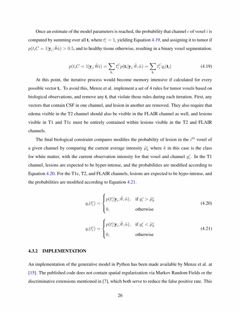
Once an estimate of the model parameters is reached, the probability that channel c of voxel i is
computed by summing over all ti where tci = 1, yielding Equation 4.19, and assigning it to tumor if
p(tiC = 1|yi; θα) > 0.5, and to healthy tissue otherwise, resulting in a binary voxel segmentation.
p(tiC = 1|yi; θα) =∑
ti
tCi p(ti|yi; θ, α) =∑
ti
tCi qi(ti) (4.19)
At this point, the iterative process would become memory intensive if calculated for every
possible vector ti. To avoid this, Menze et al. implement a set of 4 rules for tumor voxels based on
biological observations, and remove any ti that violate those rules during each iteration. First, any
vectors that contain CSF in one channel, and lesion in another are removed. They also require that
edema visible in the T2 channel should also be visible in the FLAIR channel as well, and lesions
visible in T1 and T1c must be entirely contained within lesions visible in the T2 and FLAIR
channels.
The final biological constraint compares modifies the probability of lesion in the ith voxel of
a given channel by comparing the current average intensity µck where k in this case is the class
for white matter, with the current observation intensity for that voxel and channel yci . In the T1
channel, lesions are expected to be hyper-intense, and the probabilities are modified according to
Equation 4.20. For the T1c, T2, and FLAIR channels, lesions are expected to be hypo-intense, and
the probabilities are modified according to Equation 4.21.
qi(tci) =
p(tci |yi; θ, α), if yci > µck
0, otherwise(4.20)
qi(tci) =
p(tci |yi; θ, α), if yci < µck
0, otherwise(4.21)
4.3.2 IMPLEMENTATION
An implementation of the generative model in Python has been made available by Menze et al. at
[15]. The published code does not contain spatial regularization via Markov Random Fields or the
discriminative extensions mentioned in [7], which both serve to reduce the false positive rate. This
26

algorithm was not extremely resource intensive and was run on a consumer grade Linux PC using a
quad-core CPU and 12 GB of memory. Segmentation of a single patient with 3 available modalities
only takes about 3 minutes and uses approximately 2 GB of memory. This algorithm does not use
a learning technique, so there is no lengthy training phase before segmentation can begin. This
method was designed to be applied to multimodal data containing T1, T1c, T2, and FLAIR images,
however it can accept an input of any subset of those. Patient images were segmented using each
of the 7 possible combination of input channels: T1/T2/FLAIR, T1/T2, T1/FLAIR, T2/FLAIR,
T1, T2, and FLAIR according to Table 3.
Table 3: Input data combinations possible for the Generative-Discriminative model
Input Channel Combination Censa Number of Patients Segmented
T1/T2/FLAIR 204, 214, 217, 221
T1/T2 202, 203, 204, 206, 208,214, 215, 217, 221
T1/FLAIR 201, 204, 205, 207, 210, 212, 214, 216, 217, 219, 220, 221
222, 223, 224, 225, 227, 228, 229, 303, 304, 306, 307
T2/FLAIR 204, 214, 217, 221
T1 All
T2 202, 203, 204, 206, 208,214, 215, 217, 221
FLAIR 201, 204, 205, 207, 210, 212, 214, 216, 217, 219, 220, 221
222, 223, 224, 225, 227, 228, 229, 303, 304, 306, 307
In addition to the data summarized in Table 3 the generative model was also applied to the
acute stroke datasets from ISLES 2015. Since the ISLES patients contain all three modalities each
combination of input data can be used with every patient.
According to [15] there are three requirements that the input images must meet before they
can be segmented using this algorithm: all DICOM images must be converted to NIfTI, the images
must be skull stripped, and all images, masks, and atlas maps must be in the same reference space.
27

As before, DICOM files can be converted to NIfTI easily using the MATLAB package in [14].
Skull stripping was performed partially by the LRDC, then completed using the masks they pro-
vided. All images, masks, and atlas maps were transformed to the same reference space by cross-
registering every image for a particular patient using the free software package Elastix, available
at [16], and described by [17, 18].
4.4 HISTOGRAM BASED GRAVITATIONAL OPTIMIZATION ALGORITHM
The HGOA is an interesting algorithm, but has not been developed as robustly as some of the
others so far. It has never been tested against either of the major contest datasets, and has been
designed specifically for Diffusion Weighted images.
This approach can be broken down into two components. The first attempts to segment the MRI
input using a histogram-based brain segmentation algorithm, and the second is an n-dimensional
gravitational optimization algorithm which minimizes the difference between the number of seg-
ments found in the histogram-based algorithm and the desired number of segments.
4.4.1 HISTOGRAM-BASED BRAIN SEGMENTATION
The first component of HGOA is the Histogram-Based Brain Segmentation algorithm, which is
broken down into the 7 steps shown in Figure 1 from [19].
Figure 1: Flow chart of the Histogram-Based Segmentation Algorithm.
28

First the input image is processed with a low pass Gaussian filter. Then the image intensity
histogram is calculated using Equation 4.22, where H[n] denotes the normalized histogram of the
image with a bin for each possible intensity, mn is the number of voxels with intensity n, M is the
total number of voxels in the image, and L is the number of possible intensity values.
H[n] =mn
Mn = 0, 1..L− 1 (4.22)
Step 2 is to smooth H[n] using a local weighted averaging technique, as described in Equation
4.23.
H[ni] =i+G∑i
wi ·H[ni]
G(4.23)
wi =i+G∑i
‖ni −Mw‖2 (4.24)
Where H[ni] is the local average value of the histogram, H[ni] is the histogram distribution
value of the ith bin, wi is the weight of the ith bin, andG is the length of the averaging window. The
weights for each bin are calculated using Equation 4.24, where Mw is the average of the intensities
in the window, and ni is the voxel intensity of the ith element. During this process, ifG is increased
the histogram will be smoother, and fewer local maxima will be found.
Step 3 is to locate the local maxima in the smoothed histogram using Equation 4.25.
Hmax[n] = H[ni]|(H[ni] > H[ni+1]) ∩ (H[ni] > H[ni−1]) (4.25)
In step 4 the histogram local maxima from step 3, Hmax[n] is convolved with a rectangular
window. This works upon the assumption that local intensity maxima correspond to unique brain
structures that would appear as different intensities, such as gray matter, white matter, and CSF.
Therefore, it is desired to automatically expand each local histogram maxima toward its neighbors
using the convolution described in Equation 4.26.
Y [n] = Win[n] ∗Hmax[n] =∑j
Win[j]Hmax[n− j] (4.26)
29

Where W is the length of Win[n] and M is the length of Hmax[n]. This convolution will
increase the width of each local maxima, and may result in maxima that are located close to each
other by intensity may combine into a single maximum. Due to this, a wider Win[n] will result in
fewer segments than a very narrow window.
For step 5 the upper and lower cutoff thresholds are located. This process adds additional flex-
ibility for the later optimization algorithm because increasing the threshold value T may decrease
the number of detected segments by eliminating some lower maxima. Equations 4.27 and 4.28
define the lower and upper cutoff thresholds respectively:
Xlow[ni] = {n|Y [ni+1] > T ∩ Y [ni−1] < T} (4.27)
Xhigh[ni] = {n|Y [ni−1] > T ∩ Y [ni+1] < T} (4.28)
Figure 2 demonstrates the effect that T has on the number of local maxima that are ultimately
defined to be a unique segment. Using T1 only a single segment is found, but using T2 three
segments are detected.
Step 6 defines the range of intensity values in the original image that are assigned to each
detected segment. Every voxel in the image must be assigned to a segment, and once Y [n] has
been thresholded to determine the cutoff borders of each segment there may exist gaps between
Xlow[si] and Xhigh[si+1], where si denotes the ith segment. These gaps are filled in by assigning
those intensity values to either bordering segment proportionally according to Equation 4.29.
Xhigh−new[si] = Xhigh[si] + (Xlow[si+1]−Xhigh[si])×Hmax[si]
Hmax[si] +Hmax[si+1]
Xlow−new[si+1] = Xhigh−new[si]
(4.29)
Finally, step 7 defines a specific intensity value for each detected segment. To generate the final
segmentation image, all voxels with intensity values between Xlow−new[si] and Xhigh−new[si+1] in
the original image will be converted to that respective segment’s defined intensity, Xcenter[si],
calculated using Equation 4.30.
Xcenter[si] =Xlow−new[si] +Xhigh−new[si]
2(4.30)
30

Figure 2: Example plot of Y [n] with two threshold values
4.4.2 N-DIMENSIONAL GRAVITATIONAL OPTIMIZATION ALGORITHM
Each time the 7-step process described in section 4.4.1 is performed the resulting output will be
different, and it is likely that a single iteration will not generate the desired number of segments,
or even a usable segmentation. There are three adjustable parameters that will affect the number of
segments generated in any single iteration. They are: the length of the averaging window G used
in Equations 4.23 and 4.24, the length of the convolution window Win[n] used in Equation 4.26,
and the threshold value T used in Equations 4.27 and 4.28. Since the length of both windows can
theoretically range from 1 to 256, and the threshold is defined on the interval [0, 1] it is computa-
tionally impractical to calculate a significant subset of possible combinations, and some method to
automate this process in an efficient manner is desirable.
31

The N-Dimensional Gravitational Optimization Algorithm (NGOA) is used to optimize an
objective function defined as the squared difference between the desired and achieved number of
segments. The theory behind NGOA is based on the principle of a gravitational field, functionally
it is a simulation of K particles in space, and attempts to find the heaviest.
The particles are initialized by a random selection of K n-dimensional vectors, representing
the position, velocity, and acceleration of those particles as described in Equations 4.31 through
4.33.
Xi = [[xi1, xi2, ..., xin]T (4.31)
Vi = [vi1, vi2, ..., vin]T (4.32)
ai = [ai1, ai2, ..., ain]T (4.33)
Given those parameters, the gravitational force acting upon the ith particle is calculated using
Equation 4.34.
Fi =
∏j 6=imi ·mj · (K ×Xi(t)−
∑j 6=iXj(t))∑
j 6=i((xi1 − xj1)2 + ...+ (xin − xjn)2) + Iε(4.34)
Where mi is the inverse of the value of the objective function for the ith particle since this
is a minimization problem. Once the gravitational force has been calculated, the new velocity is
calculated using Equation 4.35, and using the new velocity the new position is calculated using
Equation 4.36.
V (t+ 1)i =gai
min(aj|j=1:K)+ V (t) (4.35)
X(t+ 1)i = V (t+ 1)i +X(t)i (4.36)
In this case,N = 3, corresponding to the three parameters of the histogram based segmentation
algorithm. HGOA calculates NGOA iteratively, each time using the result to perform a histogram
based segmentation before the next iteration. This process continues until the objective function is
satisfied, the maximum number of iterations is reached, or the result of Equation 4.35 drops below
a set threshold.
32

Once the NGOA has converged, a simple thresholding operation defined by Equation 4.37 is
performed to identify the segments containing stroke lesion.
Lesion = [Xlow[si] < q1 ∩Xhigh[si] < q2] (4.37)
According to [19] q1 and q2 are defined as 2.25 and 4.85 respectively for tumor detection, and
the lesion would always be located in s2. It does not go into detail about whether these same values
were used for segmenting stroke-containing MRI. For this experiment multiple values of q1 and q2
were tested, and the restriction to segment 2 was relaxed.
4.4.3 IMPLEMENTATION
The author of HGOA has not made their source code publicly available. Since there was no source
code, a custom implementation was written using MATLAB according to the mathematical theory
published in [19], and summarized in Sections 4.4.1 and 4.4.2. HGOA does not allow multiple in-
put channels, so segmentations were only performed on each individual modality for every patient.
Running the program on a single patient takes roughly 30 seconds, however the algorithm does not
always converge in a single attempt. Typically it takes 1-2 minutes to generate a segmentation on
a typical consumer-grade CPU.
Since a custom written implementation of HGOA was used, there were no required manual
pre-processing steps. According to the figures in [3] it does not appear that Nooshin et al. were
using skull-stripped data, so the original images including the skulls were input to this algorithm.
The only remaining pre-processing performed was converting to NifTI, as they were simpler to
work with, and that conversion was necessary for the other algorithms resulting in no additional
processing time. The low pass Gaussian filter as described in [19] was applied to the input image
as the first step of the program.
33

4.5 LINDA
Pustina et al. describe the entire process to design, train, and use LINDA in [4]. In that experiment,
a set of 60 chronic stroke patients was used to train and test the algorithm, to a high degree of
success. Later it was successfully applied to a secondary dataset of 45 cases from a different lab,
made with a different scanner.
In [4] Pustina et al. propose a set of 12 features that can be calculated from each of the T1
images when developing LINDA. In the interest of computational efficiency, only the top 6 per-
forming features were included in the final LINDA algorithm. To determine the highest perfoming
features Pustina et al. use the following iterative process.
The input dataset of 60 patients was split into a training group and a test group, consisting of
48 and 12 patients respectively. Using the training group, a model was trained for each of the 12
proposed features, then that model was used to segment the 12 test patients. The Dice score was
calculated for each segmentation, and the feature with the highest aggregate score was selected.
In the next iteration only 11 models were trained, this time using the top performer from the first
iteration paired with each of the remaining 11. Those models are again tested, and the top pair is
selected, then the process repeats until no further improvement was observed. The final selected
features are as follows:
1. Subject Specific Asymmetry: Computed by reflecting the image about the Y axis, then sub-
tracting that from the original image.
2. K-Means Segmentation: Divides a collection into K groups by calculating the mean of each
group, calculating the distance between each point and mean, then re-grouping the points based
on which mean they are nearest to. This process is repeated until the sum squared error within
each group stabilizes.
3. Gradient Magnitude: Calculated as ‖( ∂I∂x, ∂I∂y, ∂I∂z
)‖ where I is the volume image. Denotes the
amount of intensity change in an image at each voxel.
4. Deviance from Control: The remaining three features are all calculated by subtracting the last
three features, from the average of that feature calculated using a group of 80 healthy control
images.
34

4.5.1 TRAINING
Pustina et al. use a multi-resolution voxel-neighborhood random forest algorithm (MRVNRF). To
build the trained model, a series of random forest models are trained at progressively increasing
resolutions. At each resolution step the random forest model is trained on a matrix containing
some feature data from all subjects. Each row pertains to a single voxel from a particular patient,
with information from each of the features arranged along the columns of that row. Random Forest
training does not require information from every single voxel, so this matrix is constructed using a
randomly selected subset of 200 voxels from each class. The ground truth for each training step is
simply each voxel’s binary lesion status, either healthy or lesion.
When training at a given resolution step is complete, the newly generated model is applied to
the training subjects to generate two new features, posterior probability maps of lesion and healthy
tissue. The next training step is the same as the first, at a higher resolution, with the posterior
probability maps from the first step as additional features. This process of training, generating
posterior probability maps, and then increasing resolution is repeated until it has been performed
for the desired number of resolution levels.
Once training is complete, the trained model can be applied to segment new subjects using a
very similar process to training. When segmenting, the posterior probabilities calculated at the end
of each resolution step are calculated by applying the previously trained model. At the end of the
highest resolution step the posterior probabilities are converted into a binary segmentation map,
assigning all voxels to a class based on which has the highest posterior probability.
4.5.2 IMPLEMENTATION
Pustina et al. have made the source code for segmentation using LINDA available to the public on-
line at [20]. This distribution comes with a model trained from a set of 60 chronic, left-hemispheric,
stroke patients from the University of Pennsylvania with T1 images. As of time of writing source
code for training new models using other, or multiple modalities had not been published online.
LINDA can be run on a typical consumer-grade CPU, however it does require a significant
amount of RAM, and is only supported on Linux. Due to these necessities all segmentations
using LINDA were performed using the high performance computing infrastructure available at
35

the University of Pittsburgh Center for Simulation and Modeling (SAM). Each segmentation was
run on a SAM computation node with 4 processor cores and 8 GB of RAM. Processing time
exhibited a high level of variance, for some patients no more than 1.5-2 hours was necessary, for
others processing time increased to roughly 8 hours. At this time it is not clear if LINDA is able to
take advantage of higher parallelization on more than 4 CPU cores for improved performance.
Since LINDA is only capable of taking a single input channel, a segmentation was attempted
with individual modalities, but was only successful with T1 images. LINDA performs most typical
pre-processing techniques such as skull-stripping and bias field correction automatically, however
according to [4] there are two pre-requisites that must be satisfied prior to using LINDA for seg-
mentation:
1. Input images must be converted to the NifTI format
2. Input images must either have a left hemispheric stroke, or if right-hemispheric be left-right
flipped. Bilateral lesions can be expected to have poor results
Requirement 1 was satisfied by converting all DICOM images to NifTI using the MATLAB
package available in [14]. All of the patients in this study had left hemispheric strokes, so no
further processing was required to fulfill requirement 2.
4.6 ANALYSIS
The output segmentation from each algorithm is a volumetric image with binary intensities. In
computational terms this is simply a 3-D matrix where every element (voxel) is either 1 or 0, with
1 denoting the lesion class, and 0 denoting the background class which includes all healthy tissue as
well. Similarly, the manual segmentations provided by the LRDC are also binary-valued matrices
that were segmented using the T1 images, resulting in a size of 192× 256× 256.
Each algorithm works in a different reference space, DeepMedic and HGOA are not depen-
dent on any particular reference space, therefore they can operate on the lesion containing images
directly, once each modality is cross registered on a per-patient basis. Prior to processing each
patient, the different modalities were registered to the T1 image using Elastix, resulting in an
36

output size of 192 × 256 × 256. LINDA automatically transforms input images to a space of
181 × 217 × 181, and provides its output in the same space. The generative model described in
Section 4.3 requires a healthy atlas for white matter, gray matter, and CSF. The atlas provided has
dimensions 160× 216× 176, requiring that all patients are transformed down to that size prior to
use, then provides an output of the same size. Prior to calculating the following statistics, copies
of the manual traces were transformed to the same size as the output from both LINDA and the
Generative model using the Transformix package in Elastix.
Most current literature, including proceedings from BRATS and ISLES, use the Sørensen-
Dice Coefficient, or Dice Score (DSC) to gauge the performance of their algorithms. The DSC
compares the similarity of two samples and will range from 0 to 1, with 1 being a perfect match.
It is frequently used in any image segmentation problem since it gives a convenient measure of the
overlap between two segmentations. DSC is calculated according to Equation 3.1. Calculating the
DSC here allows direct comparison to the performance described in other papers, and serves as an
intuitive measure of how successful each algorithm is.
Since segmentation of stroke lesions is a binary detection problem, each algorithm is essen-
tially a receiver, and there are four other statistics that are useful for characterizing a binary receiver.
Sensitivity (SEN) measures the proportion of positives that are correctly identified, Specificity
measures the proportion of negatives that are correctly identified, Accuracy measures the total pro-
portion of positive and negative results that are correct, and Precision (PRC) which measures the
proportion of true positives to the total number of positive results.
A single MRI image used here contains over 12 million total voxels. The typical large stroke
lesion will contain less than 500 thousand voxels, representing only 4% of the total image volume.
Due to this proportion, the metrics specificity and Accuracy will both represent the performance of
the algorithms very poorly since they will be greatly inflated by the large number of true negative
results, so they will not be used.
37

Formulas for Sensitivity and Precision are given as Equations 3.2 and 3.4 respectively, where
Pf is the number of false positive predictions, Nt is the number of true negative predictions, and
Nf is the number of false negative predictions. For each patient, the ground truth segmentation
and the output segmentation were read into MATLAB as 3-D matrices. Those matrices were first
processed with the round function, to guarantee that all voxels were either a 1 or 0, then Pt, Pf , Nt,
and Nf are calculated by counting the nonzero elements of the output matrices from the logical
operations shown as Equations 4.38 through 4.41 respectively.
TP = S ∧G (4.38)
TN = S ↑ G (4.39)
FP = S ∧ ¬G (4.40)
FN = ¬S ∧G (4.41)
Once the four basic cardinalities are computed, it is straightforward to calculate the Dice score,
Sensitvity, and Precision using Equations 3.1, 3.2, and 3.4 respectively.
The ISLES 2015 competetion calculated all of the previous metrics, along with two additional
ones which will be used here so that results can be compared directly, the Hausdorff Distance
(HD) and Average Symmetric Surface Distance (ASSD). The Hausdorff distance between two
finite sets A and B is defined by Equation 3.14 and the ASSD between an automatic segmentation
SA and manual segmentation SM is calculated with Equation 3.19, both the Hausdorff Distance
and the ASSD are more difficult to compute than the overlap based metrics, however since the
manual lesion traces are not available for the ISLES 2015 acute stroke data those metrics cannot
be calculated directly. Instead, the automatic segmentations were uploaded to the ISLES 2015
website, which calculates them automatically once the segmentations have been submitted.
38

5.0 RESULTS
This chapter Presents numerical results of segmentations with each algorithim on each dataset,
with some images of representative segmentations. Each of the performance metrics discussed in
Section 4.6 have been calculated for cross algorithm comparisons. Deeper discussion of the results
is found in Chapter 6.
5.1 DEEPMEDIC
When a DeepMedic model is trained using the ISLES 2015 acute stroke training data, and used to
segment the ISLES 2015 it generally performs well. Figure 3 provides a representative example of
a very successful segmentation. Image (a) of Figure 3 shows the base image before segmentation,
the lesion is most noticable along the edge of the lower right portion of the image, presenting
as mostly gray intensities, most noticable due to the asymmetry with the left side of the image.
Image (b) is the same slice of that patient’s scan with an overlay of the DeepMedic generated
segmentation. In the overlay, all of the highlighted voxels were classified as lesion by DeepMedic,
and everything else was classified as background. This image shows that DeepMedic detected the
majority of the lesion, with only a few small regions with what are likely to be false positives.
The ISLES organizers will not release the individual manual segmentations so it is difficult to be
certain if they are small lesions or false positives, however since this segmentation achieved a Dice
score of 0.9 we know it was very accurate.
A representative example of a very poor segmentation for all combinations is also proviced in
Figure 4, all trained models acheived a Dice score of 0 for this patient. In this case, the stroke lesion
appears to be located in the lower left hemisphere of the image, but presents with mostly darker
39

(a) Base Image (b) With Lesion Overlay
Figure 3: Example of DeepMedic generated segmentation on SISS patient 2, DSC = 0.9.
voxel intensities than the lesion in Figure 3. Since the manual segmentations from ISLES 2015 are
not publicly available it is impossible to be certain what voxels are considered lesion in the online
evaluation tool. This patient’s images may even be partially corrupted, as there is a small section
in the middle of what looks like lesion that has voxel intensities of exactly zero, which would be
very unusual for a medical scan.
(a) Base Image (b) With Lesion Overlay
Figure 4: Example of DeepMedic generated segmentation on SISS patient 36, DSC = 0.
40

Figure 5 shows the average Dice scores acheived by applying DeepMedic to the SISS data.
Testing with the acute SISS data showed that there was a decline in performance as input channels
were removed. The far left bar in Figure 5 labeled ”ISLES” is the result that Glocker et al entered
into ISLES 2015 and reported in [13] using 4 input modalities, all of the 3, 2, and 1 channel
models tested here performed worse than the 4 channel model, however there also appears to be
some dependance on the FLAIR channel. In these tests, the average Dice score of 0.37 for the three
channel model that used T1, T2, and FLAIR images was equivalent to the other three models that
included the FLAIR modality. Models that did not include the FLAIR modality performed strictly
worse, with an average Dice score of 0.27 for the two channel model using T1 and T2 images, then
0.22 and 0.16 for the T2 and T1 only channels respectively.
Figure 5: Average Dice Scores for DeepMedic using each combination of acute input data.
When DeepMedic was trained using the ISLES 2015 acute stroke training data, then used to
segment the chronic stroke data supplied by the LRDC average Dice scores are significantly lower
then when the training and segmentation data sets both contained acute stroke images. Figure 6
shows a typical segmentation of a chronic stroke by the three channel DeepMedic model. Image (a)
is the base image of that patient’s scan, image (b) is the same slice with overlay of the segmentation
generated by the three modality DeepMedic model. As before, the highlighted voxels in (b) were
classified by DeepMedic as lesion, and the rest were classified as background. In this case we have
41

access to the expert manual segmentation, presented as the overlay in image (c), and we can see
that even when trained with the mismatched acute data, DeepMedic is able to recognize some of
the stroke damage that appears as lighter voxel intensities in the gray range, but completely misses
the large black area that is obvious to a human observer.
(a) Base Image (b) With Lesion Overlay
(c) True Lesion
Figure 6: Representative segmentation of a chronic stroke by the 3 channel DeepMedic model
trained with acute data
Individual Dice scores for each acute image using all models are shown in Figures 7 through
9. With each model, DeepMedic segmentations displayed a high degree of variance. In all cases,
there were some patients that completely failed to segment, and some for which Dice scores of
0.8 or greater were acheived. Generally, between models the patients that DeepMedic completely
failed to segment remained the same, indicating that some stroke lesions may not present features
that DeepMedic is able to learn from the training dataset.
42

Figure 7: Individual Dice scores for all DeepMedic segmentations using the three modality model.
Similar trends were present in all metrics that were investigated. Figure 10 shows the average
Sensitivity that DeepMedic acheived when applied to the matched acute/acute training and seg-
mentation sets. In Figure 10 the far left bar is again the result published by Glocker et al in [13]
when using their four modality model on the acute ISLES 2015 data. There is generally a decline in
performance as input modalities are removed, and models containing the FLAIR images perform
strictly better than models without them, in this case the two modality T1/FLAIR and T2/FLAIR
models even have a slightly higher sensitivity than the three modality model by a small margin of
0.03 and 0.04 respectively. Since the Dice score is conveinient and easy to understand it will be
used througout the remainder of this chapter.
43

Figure 8: Individual Dice scores for all DeepMedic segmentations using the two modality models.
Figure 11 shows the average Dice score acheived by DeepMedic when segmenting the chronic
stroke images. The same general trend was present that as input image modalities were removed,
performance suffered with the exception of the T1 only case. In this experiment, there no longer
appeared to be a strong dependance on the FLAIR modality as there was in the acute case. Now
the T1 images appear to be most significant, with both T1-containing two modality models outper-
forming tthe T2/FLAIR model and the single modality T2 or FLAIR models. The T1-only model
performed suprisingly well, acheiving an average Dice score of 0.32, higher than any of the other
models when segmenting chronic data.
Figure 12 shows a segmentation of the same patient as in Figure 6, but using T1-only model,
which was the top performing model when the training and test data were mismatched. We can see
here that this model still detects most of the lesion area that the three modality model found, but
was also able to pick up some of the black region that the three modalitiy model missed completely.
44

Figure 9: Individual Dice scores for all DeepMedic segmentations using the single modality mod-
els.
Figure 13 shows the individual results for each chronic stroke patient using the top performing
T1 only DeepMedic model. Similarly to the results with the acute stroke dataset, the individual
results show a high rate of variance. Several segmentations are very successful, with Dice scores
in the 0.6-0.8 range, but many completely failed to segment with Dice scores very close to 0.
45

Figure 10: Average Sensitivity for DeepMedic acute segmentations.
Figure 11: Average Dice Scores for DeepMedic using each combination of chronic input data.
46

(a) Base Image (b) With Lesion Overlay
(c) True Lesion
Figure 12: Representative segmentation of a chronic stroke by the T1-only DeepMedic model
trained with acute data
47

Figure 13: Individual chronic segmentation results using the T1 only DeepMedic model.
48

5.2 GENERATIVE MODEL
The generative model was originally designed for acute strokes, and tested against an acute stroke
dataset in [7]. Here, it was first tested using the same acute stroke dataset that was used for
DeepMedic in section 5.1. An example segmentation by the generative model is shown in Figure
14, using the same patient as Figure 3 so that the two can be compared directly. Compared to
Figure 3 we can see that most of the lesion is still captured, however the generative model misses
some parts of it that present with lighter voxel intensities closer to white. Similarly to DeepMedic,
there were several patients that were unable to be segmented by the generative model at all. In
some cases the algorithm actually diverges and crashes, and in other cases it fails to generate
any meaningful segmentation. When applied to SISS patient number 36, the same one pictured
in Figure 4 the generative model runs successfully, but the output segmentation has no voxels
classified as lesion, resulting in a Dice score of 0.
(a) Base Image (b) With Lesion Overlay
Figure 14: Representative segmentation of an acute stroke with the generative mode, DSC = 0.61.
When applied to this acute data, the generative model underperformed the results reported in
[7], the average results are shown in Figure 15. However, this experiment was performed with a
different dataset entirely and used only up to 3 input modalities: T1, T2, and FLAIR as no T1c
49

images were available. The same general trends that were present in Section 5.1 are again present
with the generative model. As input modalities are removed, the performance of the generative
model suffers and the FLAIR images appear to be the most significant individually. Both of the
FLAIR-containing two modality tests outperform the T1/T2 set, and the single modal test with just
FLAIR performs nearly as well as the T2/FLAIR and three modality tests, outperforming both the
T1/FLAIR and T1/T2 tests.
Figure 15: Average Dice Scores for the generative model applied to acute data.
When applied to the three channel chronic stroke data, the generative model’s performance
generally declined. Figure 16 contains a segmentation created using the generative model of the
same patient used in Figure 6. Similarly to the segmentation of this patient using DeepMedic, the
generative model is able to pick up a portion of the edge of the lesion where the voxels have higher
intensities in the gray range, but misses the large black region. Figure 16 was segmented using the
generative model given three modalities: T1, T2, and FLAIR, but is similar to the segmentations
with each other subset of two or one input modality.
The average Dice scores for segmentations with the generative model using each subset of
chronic input modalities are shown in Figure 17. In this experiment there was no clear trend of
declining performance as input modalities were removed as there was with the acute stroke data.
However, the performance was generally much worse in this case since this algorithm was designed
50

for acute stroke images, and we do not have any T1c data. Between the different combinations of
input data there was a fairly small variation in performance, the top performing T2 model achieved
an average Dice score of 0.19, and the worst performing T2/FLAIR model an average of 0.09.
51

(a) Base Image (b) With Lesion Overlay
(c) True Lesion
Figure 16: Segmentation of Censa 214 with the 3 channel generative model.
52

Figure 17: Average Dice Scores for the generative model applied to chronic data.
53
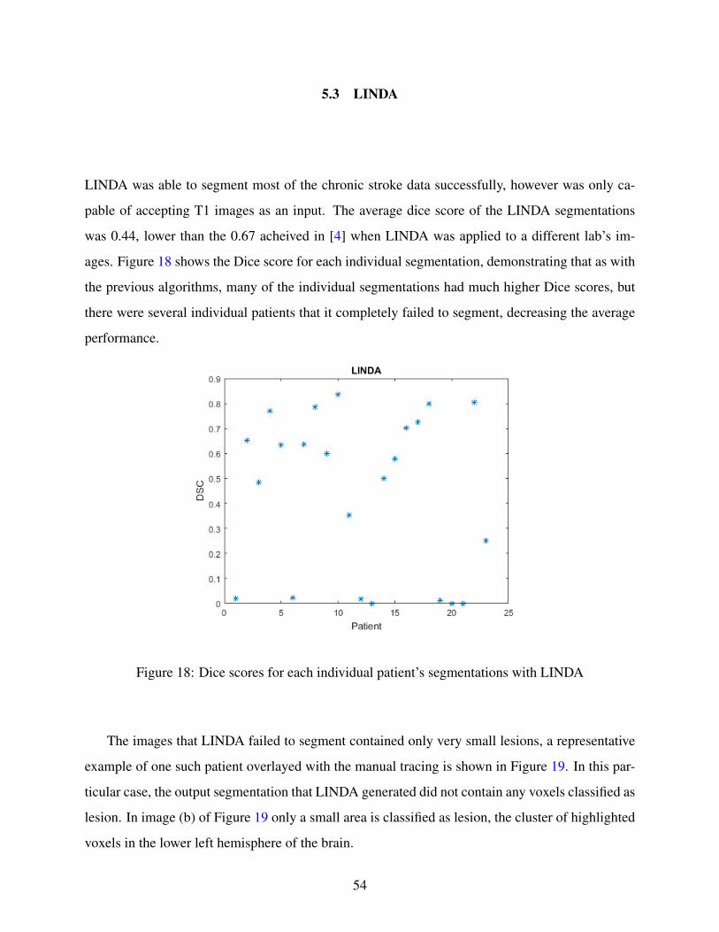
5.3 LINDA
LINDA was able to segment most of the chronic stroke data successfully, however was only ca-
pable of accepting T1 images as an input. The average dice score of the LINDA segmentations
was 0.44, lower than the 0.67 acheived in [4] when LINDA was applied to a different lab’s im-
ages. Figure 18 shows the Dice score for each individual segmentation, demonstrating that as with
the previous algorithms, many of the individual segmentations had much higher Dice scores, but
there were several individual patients that it completely failed to segment, decreasing the average
performance.
Figure 18: Dice scores for each individual patient’s segmentations with LINDA
The images that LINDA failed to segment contained only very small lesions, a representative
example of one such patient overlayed with the manual tracing is shown in Figure 19. In this par-
ticular case, the output segmentation that LINDA generated did not contain any voxels classified as
lesion. In image (b) of Figure 19 only a small area is classified as lesion, the cluster of highlighted
voxels in the lower left hemisphere of the brain.
54

(a) Base Image (b) True Lesion
Figure 19: Censa 304 image overlayed with manual segmentation, LINDA did not detect any
lesion voxels.
Figure 20 is representative of larger lesions that were segmented correctly. The publicly re-
leased model available at [20] was trained entirely with T1 images of chronic stroke patients, and
as a result LINDA does not suffer from the same issue that DeepMedic and the generative model
did where it misses legion voxels that appear as black intensities. In image (b) of Figure 20 we can
see that LINDA identified nearly the entire lesion as shown in image (c). There is a small lesion
area in the lower left hemisphere separated from the large one that LINDA misses entirely, and
there are some false positive regions in the large continuous lesion in the upper left hemisphere. In
this example LINDA achieved a Dice score of 0.8, reduced mostly by the false positive regions.
55

(a) Base Image (b) With Lesion Overlay
(c) True Lesion
Figure 20: Segmentation of Censa 306 with LINDA.
56

5.4 HGOA
The HGOA algorithm was not able to produce any useful segmentations using either the chronic
or acute datasets. In [19] values of 2.25 and 4.85 for q1 and q2 in Equation 4.37 were used to detect
a lesion segment. In testing the algorithm, generated segments were never able to satisfy that
requirement, and no other values for q1 and q2 that worked in general could be identified. Looking
at many of the segmentations it was apparent that it would be difficult for any available patients to
meet these criteria since the lesions typically spanned a larger range of intensity values.
An example segmentation of a chronic stroke patient using HGOA is provided in Figure 21.
In this example, HGOA was run with a target of 5 segments, and none of the resultant segments
satisfied Equation 4.37 using the values given in [19]. Image (a) in Figure 21 shows the original
T1 scan, and images (b) through (f) show the five unique segments that the HGOA algorithm
identified. In this example, some lesion voxels are distributed between all 5 segments; most of the
lesion is contained in segments 1, 2, and 3, with only small portions being identified in segments 4
and 5. While segment 1 contained the single largest concentration of lesion voxels, without finding
some general criteria that satisfy Equation 4.37 there is no objective way to automatically classify
any segment as lesion. Selecting segment 1 as lesion in this case would in fact be a violation of
another restriction detailed in [19] that requires the lesion to always be located in segment 2.
57

(a) Base Image (b) Segment 1
(c) Segment 2 (d) Segment 3
(e) Segment 4 (f) Segment 5
Figure 21: Example segmentation of Censa 214 with HGOA
58

6.0 DISCUSSION
This chapter provides further qualitative analysis based on the results presented in Chapter 5. A
basic conclusion regarding the effects of limited modality data on the DeepMedic models and jus-
tification for why the generative model and HGOA algorithms were unsuccessful with the chronic
data is presented. We also discuss the performance of each algorithm on chronic and stroke data,
then finally suggest two possible avenues for extending this research.
6.1 PERFORMANCE AS INPUT DATA IS REDUCED
When applied to the matched acute training and testing data from ISLES 2015, DeepMedic demon-
strated a reduction in performance as input modalities were removed. In [13] DeepMedic was
reported to achieve an average Dice score of 0.59 when using all 4 channels: T1, T1c, T2, and
FLAIR. When tested here with three channels, removing T1c, it achieves an average Dice score
of 0.37. When the FLAIR channel was removed for the T1/T2 model the average Dice score
dropped again to 0.27, and either T2 or T1 alone achieved averages of 0.22 and 0.16 respectively.
Interestingly, combinations of T1 and FLAIR, T2 and FLAIR, or even FLAIR alone achieved the
same average Dice score as the three-channel model, 0.37. This suggests that while performance
certainly tends to drop as channels are removed, this algorithm may be overly tuned for T1c and
FLAIR data, as any models containing those modalities performed the best, or that T1c and FLAIR
imaging are inherently more valuable for viewing stroke lesions.
Results using the generative model to segment the acute ISLES 2015 data were consistent with
those of DeepMedic. The algorithm generally lost performance as the number of input channels
was reduced, and showed some dependence on the FLAIR images. The top performer was the
59

three channel combination with an average Dice score of 0.25. All of the two channel combina-
tions performed worse, but with both combinations that included FLAIR images performing better
than the T1/T2 combination. T2/FLAIR and T1/FLAIR achieved average Dice scores of 0.21 and
0.14 respectively, T1/T2 performed significantly worse with an average score of only 0.04. Gen-
erally, this algorithm performed even worse with only one channel, however the FLAIR only test
performed surprisingly well with an average score of 0.19, almost as high as theT2/FLAIR com-
bination. Again, this result suggests that FLAIR images are especially important to the success of
the generative model, as they were with DeepMedic. At time of writing no segmentation results
of the acute ISLES 2015 data have been published, but in [7] this algorithm was tested using a
different 4 channel acute stroke dataset and reported average Dice scores of up to 0.78.
When applied to the chronic dataset, both DeepMedic and the generative model, showed gen-
erally poor performance. The low performance in these cases can be partially explained by mis-
matched disease states. Both DeepMedic and the generative model were designed for acute stroke
images, which typically appear with different voxel intensities than chronic stroke damage. Addi-
tionally, the DeepMedic models used here were trained with all acute stroke data since not enough
chronic data was available for training a model, resulting in models that would be looking for
characteristics of acute strokes that may not be generalizable to chronic strokes.
However, DeepMedic still showed a general decrease in performance as the number of input
modalities was reduced. The DeepMedic model trained with three modalities achieved an average
Dice score of 0.2, and the two worst performers T2 and FLAIR achieved average Dice scores of
0.05 and 0.06 There was one exception, the T1 only model achieved an average Dice score of 0.32,
since all DeepMedic models were trained using acute stroke data it is unlikely for these results to
be reliable in general.
Using the chronic dataset, the generative model did not show the same decrease as input modal-
ities were removed. These results suggest that the T2 weighted images are the most useful, as T2
and the combination of T1 and T2 were the top two performers. However, all data combinations
performed poorly with average Dice scores ranging from 0.1 to 0.18.
60

6.2 SEGMENTATION FAILURES WITH THE GENERATIVE MODEL
The generative model performed significantly worse than was reported in [7], which ranged from
Dice scores of 0.5 to 0.8 when the model was generalized to their stroke dataset. There are several
factors that may be related to the decreased performance. Most notably, the only change made
to the algorithm in [7] when applying it to the stroke data was to remove the requirement that all
lesions in T1c images must be contained within lesions detected in the T2 and FLAIR channels.
This suggests that the generative model may be particularly reliant on T1c data, which was not
available for these experiments.
Additionally, the code for this algorithm that was made available at [15] was not the complete
code tested in [7]. It was missing spatial regularization through Markov Random Fields, and part
of the discriminative model extensions, which were the two main contributions of [7]. Markov
Random Fields especially were shown to greatly reduce the error rate, and thus increase the Dice
score of the final segmentation.
6.3 SEGMENTATION FAILURES WITH DEEPMEDIC
When applied to the acute dataset, DeepMedic exhibited a high variance with each model. Looking
at results with the three-channel model there are some patients that DeepMedic achieved a very
high Dice score of 0.9, while there are also several that had Dice scores of 0. Some of those
low scoring patients had lesions that appeared similar to a chronic stroke lesion such as the image
provided as Figure 4. In that patient, the lesion area appears with low intensity values, closer to
0, whereas most of the acute stroke images present with high intensity values closer to 1, and
Chronic stroke lesions tend to present low intensity lesions as well. The remaining low scoring
patients have very small lesions, suggesting that DeepMedic also has difficulty learning features
that successfully detect very small lesions.
61

6.4 LINDA LIMITATION TO T1 AND CHRONIC IMAGES
Since the publicly available LINDA model was trained with only T1 images containing chronic
stroke lesions, it could not be tested with T2, FLAIR, or multi-modal data. Testing it with the
T1 data available, LINDA achieved an average Dice score of 0.44. This data was generated at
a different lab with a different scanner than the data used to train LINDA and exhibited a Dice
reduction greater than the 0.02 reported in [4] where Pustina et al. postulate that this small drop
means LINDA is very generalizable to other labs data. However, in this test the greater drop may
be better explained by the individual results. Some patients lesions were successfully segmented
with Dice scores ranging from 0.8 to 0.9, and there were several that were complete failures with
a Dice score of 0. Most of these failed patients had very small lesions, such as the one shown in
Figure 19. suggesting that LINDA is simply unable to find these extremely small lesions.
6.5 SEGMENTATION FAILURES WITH HGOA
It is difficult to diagnose why this implementation of HGO was not able to generate any useful
segmentations. Since the one used here was written based on the description in [19] as opposed
to having the original source code it is possible that some error was made during writing, such
as making a mistake in one of the Histogram-based segmentation steps, or making an inaccurate
assumption. Likewise, there are several key parameters used in the algorithm that are not described
extensively in that document. After each of the first several iterations of the algorithm a random
function is added to the image that is reported to greatly increase the likelihood of the optimization
algorithm converging, and therefore generating a segmentation. Very little detail about this random
function is given, making it difficult to duplicate independantly.
62

It is also likely that this algorithm is highly specific to DWI images. If the iterative HGOA
process converges the output segmentation will contain the number of segments that the objective
function was set to look for at the beginning. The algorithm then assigns each segment to either
healthy or lesion based on the intensity width. Nabizadeh simply defines the lesion segment width
to be 1.8, with little explanation of how that number was reached. It is likely that number is very
dependant on the type of modality being used, and would be difficult to pick an appropriate value
for other modalities without extensive testing.
6.6 FURTHER RESEARCH
The main avenue for further research is related to DeepMedic’s performance on the chronic stroke
dataset. Since there were only 24 patients with Chronic strokes available, and only a small subset
of those had FLAIR, T1, and T2 data available there was a limited amount of testing possible. With
such a small dataset, it is not practical to divide it into training and testing data of any significant
size. Ideally, with a chronic stroke dataset at least double in size new DeepMedic models could be
trained to test see if its difficulty identifying chronic stroke data is inherent to the algorithm itself,
or due to the fact that the models used here were trained with acute stroke images.
Additionally, LINDA was only trained using T1 data, and unable to segment any other modal-
ities. Pustina et al. indicate in [20] that they may make training scripts for new LINDA models
available to other research groups in the future. They also indicate that to successfully train a new
model at least 30 images must be available, so a large dataset of multi-modal data would also al-
low for creating new LINDA models using the other image modalities, and possibly a multi-modal
LINDA model.
63

APPENDIX
DEEPMEDIC CONFIGURATION FILES
This Appendix contains copies of the DeepMedic configuration files used to create and train the 3
channel models used in this paper. They can easily be adjusted for a different number of channels
by adjusting the variable numberOfInputChannels in the model configuration file, and adding or
remocing arguments to the channels variable in the training file. Section A.1 contains a configu-
ration file that controls various model level parameters such as the number of layers and feature
maps per layer. Section A.2 contains a the configuration file read by DeepMedic at training time
and controls parameters such as the dropout anjd learning rates.
Most of both configuration files are identical to the default ones distributed with the DeepMedic
source code at [12], with changes to some values for better segmentation of stroke data as described
in [13].
A.1 MODEL CREATION
# D e f a u l t v a l u e s are s e t i n t e r n a l l y , i f t h e c o r r e s p o n d i n g
parame te r i s n o t found i n t h e c o n f i g u r a t i o n f i l e .
# [ O p t i o n a l b u t h i g h l y s u g g e s t e d ] The name w i l l be used i n t h e
f i l e n a m e s when s a v i n g t h e model .
64

# D e f a u l t : ”cnnModel”
modelName = ” deepMedic−FULL”
# [ R e q u i r e d ] The main f o l d e r t h a t t h e o u t p u t w i l l be p l a c e d .
f o l d e r F o r O u t p u t = ” . . / . . / . . / o u t p u t / ”
#================ MODEL PARAMETERS =================
# [ R e q u i r e d ] The number o f c l a s s e s i n t h e t a s k . I n c l u d i n g
background !
numberOfOutpu tC la s se s = 2
# [ R e q u i r e d ] The number o f i n p u t channe l s , eg number o f MRI
m o d a l i t i e s .
numberOf Inpu tChanne l s = 3
#+++++++++++Normal pathway+++++++++++
# [ R e q u i r e d ] T h i s l i s t s h o u l d have as many e n t r i e s as t h e number
o f l a y e r s I want t h e normal−pathway t o have .
#Each e n t r y i s an i n t e g e r t h a t s p e c i f i e s t h e number o f F e a t u r e
Maps t o use i n each o f t h e l a y e r s .
numberFMsPerLayerNormal = [ 3 0 , 30 , 40 , 40 , 40 , 40 , 50 , 50]
# [ R e q u i r e d ] T h i s l i s t s h o u l d have as many e n t r i e s as t h e number
o f l a y e r s i n t h e normal pathway .
#Each e n t r y s h o u l d be a s u b l i s t w i t h 3 e n t r i e s . These s h o u l d
s p e c i f y t h e d i m e n s i o n s o f t h e k e r n e l a t t h e c o r r e s p o n d i n g
l a y e r .
kerne lDimPerLayerNormal = [ [ 3 , 3 , 3 ] , [ 3 , 3 , 3 ] , [ 3 , 3 , 3 ] , [ 3 , 3 , 3 ] ,
[ 3 , 3 , 3 ] , [ 3 , 3 , 3 ] , [ 3 , 3 , 3 ] , [ 3 , 3 , 3 ] ]
65

#+++++++++++Subsampled pathway+++++++++++
# [ O p t i o n a l ] S p e c i f y whe ther t o use a subsampled pathway . I f False
, a l l subsampled−r e l a t e d p a r a m e t e r s w i l l be read b u t
d i s r e g a r d e d i n t h e model−c o n s t r u c t i o n .
# D e f a u l t : F a l s e
useSubsampledPathway = True
# [ O p t i o n a l s ] The below p a r a m e t e r s s p e c i f y t h e subsampled−pathway
a r c h i t e c t u r e i n a s i m i l a r way as t h e normal .
# I f t h e y are ommi t t ed and useSubsampledPathway i s s e t t o True ,
t h e subsampled pathway w i l l be made s i m i l a r t o t h e normal
pathway ( s u g g e s t e d f o r easy use ) .
# [WARN] Subsampled pathway MUST have t h e same s i z e o f r e c e p t i v e
f i e l d as t h e normal . L i m i t a t i o n i n t h e code . User c o u l d e a s i l y
s p e c i f y d i f f e r e n t number o f FMs . But care must be g i v e n i f
number o f l a y e r s i s changed . In t h i s case , k e r n e l s i z e s s h o u l d
a l s o be a d j u s t e d t o a c h i e v e same s i z e o f Rec . F i e l d .
numberFMsPerLayerSubsampled = [ 3 0 , 30 , 40 , 40 , 40 , 40 , 50 , 50]
ke rne lDimPerLayerSubsampled = [ [ 3 , 3 , 3 ] , [ 3 , 3 , 3 ] , [ 3 , 3 , 3 ] ,
[ 3 , 3 , 3 ] , [ 3 , 3 , 3 ] , [ 3 , 3 , 3 ] , [ 3 , 3 , 3 ] , [ 3 , 3 , 3 ] ]
# [ O p t i o n a l ] How much t o downsample t h e image t h a t t h e subsampled−
pathway p r o c e s s e s .
# D e f a u l t : [ 3 , 3 , 3 ]
s u b s a m p l e F a c t o r = [ 3 , 3 , 3 ]
#+++++++++++E x t r a FC Lay er s+++++++++++
# [ O p t i o n a l ] A f t e r t h e l a s t l a y e r s o f t h e normal and subsampled
pathways are c o n c a t e n a t e d , a d d i t i o n a l F u l l y Connec ted l a y e r s
can be added b e f o r e t h e f i n a l c l a s s i f i c a t i o n l a y e r .
66

# S p e c i f y a l i s t , w i t h as many e n t r i e s as t h e number o f ADDITIONAL
FC l a y e r s ( o t h e r than t h e c l a s s i f i c a t i o n l a y e r ) t o add . The
e n t r i e s s p e c i f y t h e number o f F e a t u r e Maps t o use .
# D e f a u l t : [ ]
numberFMsPerLayerFC = [ 1 5 0 , 150]
#+++++++++++S i z e o f Image Segments+++++++++++
# DeepMedic does n o t p r o c e s s p a t c h e s o f t h e image , b u t l a r g e r
image−s e g m e n t s . S p e c i f y t h e i r s i z e here .
# [ R e q u i r e d ] S i z e o f t r a i n i n g s e g m e n t s i n f l u e n c e t h e c a p t u r e d
d i s t r i b u t i o n o f samp les from t h e d i f f e r e n t c l a s s e s ( s e e
DeepMedic paper )
segmentsDimTra in = [ 2 5 , 2 5 , 2 5 ]
# [ O p t i o n a l ] The s i z e o f s e g m e n t s t o use d u r i n g t h e v a l i d a t i o n −on−
sample s p r o c e s s t h a t i s per fo rmed t h r o u g h o u t t r a i n i n g i f
r e q u e s t e d .
# D e f a u l t : e q u a l t o r e c e p t i v e f i e l d , t o v a l i d a t e on p a t c h e s .
segmentsDimVal = [ 1 7 , 1 7 , 1 7 ]
# [ O p t i o n a l ] B ig ge r image s e g m e n t s f o r I n f e r e n c e are s a f e t o use
and o n l y speed up t h e p r o c e s s . Only l i m i t a t i o n i s t h e GPU
memory .
# D e f a u l t : e q u a l t o t h e t r a i n i n g segment .
s e g m e n t s D i m I n f e r e n c e = [ 4 5 , 4 5 , 4 5 ]
#+++++++++++Batch S i z e s+++++++++++
# [ R e q u i r e d ] The number o f s e g m e n t s t o c r e a t e a b a t c h .
#The samples i n a t r a i n i n g−b a t c h are a l l p r o c e s s e d and one
o p t i m i z a t i o n s t e p i s per fo rmed .
# Larger b a t c h e s a p p r o x i m a t e t h e t o t a l da ta b e t t e r and s h o u l d
67

p o s i t i v e l y i mp ac t o p t i m i z a t i o n b u t are c o m p u t a t i o n a l l y more
e x p e n s i v e ( t i m e and memory ) .
b a t c h S i z e T r a i n = 10
# [ O p t i o n a l s ] Batch s i z e s f o r v a l i d a t i o n and i n f e r e n c e o n l y
i n f l u e n c e t h e speed . The b i g g e r t h e b e t t e r . Depends on t h e
segment s i z e and t h e model s i z e how b i g b a t c h e s can be f i t i n
memory .
# D e f a u l t : Equal t o t r a i n−b a t c h s i z e .
b a t c h S i z e V a l = 48
b a t c h S i z e I n f e r = 10
# [ O p t i o n a l s ] Dropout R a t e s on t h e i n p u t c o n n e c t i o n s o f t h e
v a r i o u s l a y e r s . Each l i s t s h o u l d have as many e n t r i e s as t h e
number o f l a y e r s i n t h e c o r r e s p o n d i n g pathway .
# 0 = no d r o p o u t . 1= 100% drop o f t h e neurons . Empty l i s t f o r no
d r o p o u t .
# D e f a u l t : [ ]
d r o p o u t R a t e s N o r m a l = [ ]
d r o p o u t R a t e s S u b s a m p l e d = [ ]
# D e f a u l t : 50% d r o p o u t on e v e r y F u l l y Connec ted l a y e r e x c e p t f o r
t h e f i r s t one a f t e r t h e c o n c a t e n a t i o n
# Note : The l i s t f o r FC r a t e s s h o u l d have one a d d i t i o n a l e n t r y i n
compar i son t o ”numberFMsPerLayerFC ” , f o r t h e c l a s s i f i c a t i o n
l a y e r .
d r o p o u t R a t e s F c = [ 0 . 0 , 0 . 5 , 0 . 5 ] # +1 f o r t h e c l a s s i f i c a t i o n
l a y e r !
# [ O p t i o n a l s ] R e g u l a r i z a t i o n L1 and L2 .
# D e f a u l t s : L1 reg = 0 . 0 0 0 0 0 1 , L2 reg = 0 .0001
L1 reg = 0 .000001
68

L2 reg = 0 .0001
# [ O p t i o n a l ] I n i t i a l i z a t i o n method o f t h e k e r n e l w e i g h t s . S p e c i f y
0 f o r c l a s s i c , from t h e normal d i s t r i b u t i o n N( 0 , 0 . 0 1 ) .
O t h e r w i s e s p e c i f y 1 f o r t h e method o f He e t a l from ” D e l v i n g
Deep i n t o R e c t i f i e r s ” .
# D e f a u l t : 1
i n i t i a l i z e C l a s s i c 0 o r D e l v i n g 1 = 1
# [ O p t i o n a l ] A c t i v a t i o n F u n c t i o n f o r a l l c o n v o l u t i o n a l l a y e r s .
S p e c i f y 0 f o r ReLU , 1 f o r PreLU .
# D e f a u l t : 1
r e l u 0 o r P r e l u 1 = 0
# [ O p t i o n a l ] Batch N o r m a l i z a t i o n u s e s a r o l l i n g average o f t h e mus
and s t d f o r i n f e r e n c e . S p e c i f y ove r how many b a t c h e s (
o p t i m i z a t i o n s t e p s ) t h i s r o l l i n g average s h o u l d be t a k e n .
# D e f a u l t : 60 ( i n our u s u a l s e t t i n g s , w i t h b a t c h s i z e =10 , s e g m e n t s
per t r a i n i n g subepoch =1000 , and subepochs per epoch =20 , t h i s
a v e r a g e s over 5 epochs ) .
ro l lAverageForBNOverTha tManyBatches = 60
#+++++++++++O p t i m i z a t i o n+++++++++++
# [ O p t i o n a l s ]
# I n i t i a l L e a rn i n g Rate . D e f a u l t : 0 . 0 0 1 .
l e a r n i n g R a t e = 0 . 0 1
# O p t i m i z e r t o use . 0 f o r c l a s s i c SGD, 1 f o r Adam , 2 f o r RmsProp .
D e f a u l t : 2
sgd0orAdam1orRms2 = 2
# Type o f momentum t o use . 0 f o r s t a n d a r d momentum , 1 f o r N e s t e r o v
69

. D e f a u l t : 1
c las s i cMom0OrNes te rov1 = 1
#Momentum Value t o use . D e f a u l t : 0 . 6
momentumValue = 0 . 6
#Non−Normal i zed ( 0 ) or Normal i z ed momentum ( 1 ) . Bear i n mind t h a t
Normal i z ed mom may r e s u l t i n s m a l l e r g r a d i e n t s and migh t need
r e l a t i v e l y h i g h e r L e a rn i n g Rate . D e f a u l t : 1
momNonNorm0orNormalized1 = 1
# Parame ter s f o r RmsProp . D e f a u l t : rho =0 .9 , e =10∗∗(−4) (1 e−6 blew
up t h e g r a d i e n t s . Haven ’ t t r i e d 1e−5 y e t ) .
rhoRms = 0 . 9
eps i lonRms = 10∗∗(−4)
A.2 TRAINING
# D e f a u l t v a l u e s are s e t i n t e r n a l l y , i f t h e c o r r e s p o n d i n g
parame te r i s n o t found i n t h e c o n f i g u r a t i o n f i l e .
# [ O p t i o n a l b u t h i g h l y s u g g e s t e d ] The name w i l l be used f o r s a v i n g
t h e models , l o g s and r e s u l t s .
# D e f a u l t : ” t r a i n S e s s i o n ”
sess ionName = ” t r a i n S e s s i o n D e e p M e d i c−FULL”
# [ R e q u i r e d ] The main f o l d e r t h a t t h e o u t p u t w i l l be p l a c e d .
f o l d e r F o r O u t p u t = ” . . / . . / . . / o u t p u t / ”
# [ O p t i o n a l ] The pa th t o t h e saved CNN−model t o use f o r t r a i n i n g .
O p t i o n a l i n t h e case t h e t h e model i s s p e c i f i e d from command
l i n e w i t h t h e −model o p t i o n . In t h i s case , t h i s e n t r y f i l e o f
t h e c o n f i g f i l e w i l l be d i s r e g a r d e d , and t h e one from t h e
70

command l i n e w i l l be used .
c n n M o d e l F i l e P a t h = ” . . / . . / . . / o u t p u t / models / p l a c e h o l d e r ”
#=======================T r a i n i n g
=====================================
#+++++++++++I n p u t+++++++++++
# [ R e q u i r e d ] A l i s t t h a t s h o u l d c o n t a i n as many e n t r i e s as t h e
c h a n n e l s o f t h e i n p u t image ( eg m u l t i−modal MRI ) . The e n t r i e s
s h o u l d be p a t h s t o f i l e s . Those f i l e s s h o u l d be l i s t i n g t h e
p a t h s t o t h e c o r r e s p o n d i n g c h a n n e l s f o r each t r a i n i n g−case . (
s e e example f i l e s ) .
c h a n n e l s T r a i n i n g = [ ” . / t r a i n C h a n n e l s f l a i r . c f g ” , ” . /
t r a i n C h a n n e l s t 1 c . c f g ” , ” . / t r a i n C h a n n e l s t 2 . c f g ” ]
# [ R e q u i r e d ] The pa th t o a f i l e which s h o u l d l i s t p a t h s t o t h e
Ground T r u t h l a b e l s o f each t r a i n i n g case .
g t L a b e l s T r a i n i n g = ” . / t r a i n G t L a b e l s . c f g ”
#+++++++++++Sampl ing+++++++++++
# [ O p t i o n a l ] The pa th t o a f i l e , which s h o u l d l i s t p a t h s t o t h e
Region−Of− I n t e r e s t masks f o r each t r a i n i n g case .
# I f ROI masks are prov ided , under d e f a u l t−s a m p l i n g s e t t i n g s , t h e
t r a i n i n g sample s w i l l be e x t r a c t e d o n l y w i t h i n i t . O t h e r w i s e
from whole volume .
# T h i s mask i s a l s o used f o r c a l c u l a t i n g mu and s t d i n t e n s i t i e s
f o r i n t e n s i t y −augmen ta t ion , i f pe r fo rmed .
71

# r o i M a s k s T r a i n i n g = ” . / t r a i n R o i M a s k s . c f g ”
# [ O p t i o n a l ] The p e r c e n t a g e o f t r a i n i n g samples t o e x t r a c t from
f o r e g r o u n d (GT− l a b e l s ) .
# D e f a u l t : 0 . 5
p e r c e n t O f S a m p l e s T o E x t r a c t P o s i t i v e T r a i n = 0 . 5
#+++++++++++Advanced Sampl ing+++++++++++
# [ O p t i o n a l ] True i n o r d e r t o use d e f a u l t s a m p l in g f o r t r a i n i n g .
In t h i s case , p o s i t i v e sample s are e x t r a c t e d from w i t h i n t h e
GT mask .
# N e g a t i v e samples are t h e n e x t r a c t e d from t h e ROI ( or f u l l volume
) , e x c l u d i n g t h e GT .
#NOTE: Advanced o p t i o n s are d i s a b l e d i f d e f a u l t s e t t i n g s are used
.
# D e f a u l t : True
useDefau l tT ra in ingSampl ingFromGtAndRo i = True
”””
#++Adv . Sampl . O p t i o n s . These are d i s a b l e d i f Using−D e f a u l t−
T r a i n i n g−Sampl ing .++
# Weight−maps , t h a t w i l l d e f i n e a r e a s o f t h e image t o sample more .
S e p a r a t e f o r t r a i n i n g and n e g a t i v e sample s .
# Note : Weight−maps don t have t o be n o r m a l i z e d .
# I m p l e m e n t a t i o n Note : I n t e r n a l l y , t h e s e are what i s a c t u a l l y used
f o r s am p l i n g . Under d e f a u l t s e t t i n g s , t h e pos−weigh t−map i s
pa s s ed GT−l a b e l s , neg−weigh t−map pa ss ed t h e ROI .
# we igh tedMapsForPosSampl ingTra in = ” . / t r a i n G t L a b e l s . c f g ”
# weigh tedMapsForNegSampl ingTra in = ” . / t r a i n R o i M a s k s . c f g ”
72

# S p e c i f y i f t h e we igh t−maps are a c t u a l l y w e i g h t s ( True ) . I f False
, we assume t h e y are GT / ROI . And s u b t r a c t GT from ROI t o do
t h e n e g a t i v e−s a m p l i n g .
sampl ingMasksAreProbMapsTrain = F a l s e
”””
#+++++++++++T r a i n i n g Cyc le ( s e e d o c u m e n t a t i o n )+++++++++++
# [ O p t i o n a l s b u t h i g h l y s u g g e s t e d as t h e y are model d e p e n d e n t . ]
#How many epochs t o t r a i n f o r . D e f a u l t : 35
numberOfEpochs =35
#How many subepochs c o m p r i s e an epoch . Every subepoch I g e t
Accuracy r e p o r t e d . D e f a u l t : 20
numberOfSubepochs = 20
# Every subepoch , l oad t h e images from t h a t many c a s e s and e x t r a c t
new t r a i n i n g sample s . D e f a u l t : 50
numOfCasesLoadedPerSubepoch = 50
# Every subepoch , e x t r a c t i n t o t a l t h i s many s e g m e n t s and load
them on t h e GPU. Memory L i m i t a t e d . D e f a u l t : 1000
# Note : T h i s number i n c o m b i n a t i o n w i t h t h e b a t c h S i z e T r a i n i n g ,
d e f i n e t h e number o f o p t i m i z a t i o n s t e p s per subepoch (=
NumOfSegmentsOnGpu / B a t c h S i z e ) .
numberTrain ingSegmentsLoadedOnGpuPerSubep = 1000
#+++++++++++L e a r n i n g Rate S c h e d u l e+++++++++++
# [ O p t i o n a l ] The t y p e o f s c h e d u l e t o use f o r L e a r n in g Rate
a n n e a l i n g .
#0= S t a b l e Decrease . 1=Auto ( Lower LR when v a l i d a t i o n a c c u r a c y
p l a t e a u s . R e q u i r e s v a l i d a t i o n −on−sample s ) . 2=Lower a t
73

p r e d e f i n e d epochs . 3= E x p o n e n t i a l l y d e c r e a s e LR , l i n e a r l y
i n c r e a s e Mom.
#NOTE: T r a i n i n g S c h e d u l e i s v e r y i m p o r t a n t . We s u g g e s t r u n n i n g
s t a b l e and o b s e r v i n g t r a i n i n g e r r o r , t h e n lower LR when i t
p l a t e a u s . Otherwise , use e x p o n e n t i a l b u t make s u r e t o t r a i n
f o r enough epochs .
s t a b l e 0 o r A u t o 1 o r P r e d e f i n e d 2 o r E x p o n e n t i a l 3 L r S c h e d u l e = 2
# [ For S t a b l e + Auto + P r e d e f i n e d ] By how much t o d i v i d e LR when
l o w e r i n g . D e f a u l t : 2
whenDecreas ingDiv ideLrBy = 2 . 0
# [ For S t a b l e + Auto ] How many epochs t o w a i t b e f o r e d e c r e a s i n g
aga in . S e t Zero t o n e v e r lower LR . D e f a u l t : 3
# numEpochsToWai tBeforeLower ingLr = 3
# [ For Auto ] I f v a l i d a t i o n a c c u r a c y i n c r e a s e s more than t h i s much ,
r e s e t t h e w a i t i n g c o u n t e r . D e f a u l t : 0 .0005
# m i n I n c r e a s e I n V a l i d a t i o n A c c u r a c y T h a t R e s e t s W a i t i n g = 0 .0005
# [ R e q u i r e d f o r P r e d e f i n e d ] At which epochs t o lower LR .
p r e d e f i n e d S c h e d u l e = [ 1 2 , 16 , 19 , 22 , 25 , 28 , 31 , 34 , 37 , 40 , 43 ,
46]
# [ R e q u i r e d f o r E x p o n e n t i a l ] [ F i r s t epoch t o s t a r t l o w e r i n g from ,
v a l u e f o r LR t o reach a t l a s t epoch , v a l u e f o r Mom t o reach a t
l a s t epoch ]
exponent ia lSchedForLrAndMom = [ 1 2 , 1 . 0 / ( 2 ∗ ∗ ( 7 ) ) , 0 . 9 ]
#+++++++++++Data Augmen ta t ion+++++++++++
74

# [ O p t i o n a l ] S p e c i f y whe ther t o r e f l e c t t h e images by 50%
p r o b a b i l i t y i n r e s p e c t t o t h e X / Y / Z a x i s . D e f a u l t : [ False ,
False , F a l s e ]
r e f l e c t I m a g e s P e r A x i s = [ True , F a l s e , F a l s e ]
# [ O p t i o n a l ] Augmen ta t ion by chang ing t h e mean and s t d o f t r a i n i n g
sample s . D e f a u l t : F a l s e
performIntAugm = F a l s e
# I ’ = ( I + s h i f t ) ∗ m u l t i
# [ O p t i o n a l s ] We sample t h e ” s h i f t ” and ” m u l t i ” v a r i a b l e f o r each
sample from a Gauss ian d i s t r i b u t i o n . S p e c i f y t h e mu and s t d .
# D e f a u l t s : [ 0 , 0 . 1 ] and [ 1 . , 0 . ]
sampleIntAugmShif tWithMuAndStd = [ 0 , 0 . 1 ]
sampleIntAugmMultiWithMuAndStd = [ 1 . , 0 . 0 ]
#==================V a l i d a t i o n=====================
# [ O p t i o n a l s ] S p e c i f y whe ther t o per fo rm v a l i d a t i o n on samples and
f u l l −i n f e r e n c e e v e r y few epochs . D e f a u l t : F a l s e f o r bo th .
p e r f o r m V a l i d a t i o n O n S a m p l e s T h r o u g h o u t T r a i n i n g = F a l s e
p e r f o r m F u l l I n f e r e n c e O n V a l i d a t i o n I m a g e s E v e r y F e w E p o c h s = True
# [ R e q u i r e d ] S i m i l a r t o c o r r e s p o n d i n g parame te r f o r t r a i n i n g , b u t
p o i n t s t o c a s e s f o r v a l i d a t i o n .
c h a n n e l s V a l i d a t i o n = [ ” . / v a l i d a t i o n / v a l i d a t i o n C h a n n e l s f l a i r . c f g ”
, ” . / v a l i d a t i o n / v a l i d a t i o n C h a n n e l s t 1 c . c f g ” , ” . / v a l i d a t i o n /
v a l i d a t i o n C h a n n e l s t 2 . c f g ” ]
# [ R e q u i r e d f o r v a l i d a t i o n on samples , o p t i o n a l f o r f u l l −i n f e r e n c e
75

] S i m i l a r t o c o r r e s p o n d i n g parame te r f o r t r a i n i n g , b u t p o i n t s
t o c a s e s f o r v a l i d a t i o n .
g t L a b e l s V a l i d a t i o n = ” . / v a l i d a t i o n / v a l i d a t i o n G t L a b e l s . c f g ”
# [ R e q u i r e d ] S i m i l a r t o c o r r e s p o n d i n g parame te r f o r t r a i n i n g . Only
i n f l u e n c e s how a c c u r a t e l y t h e v a l i d a t i o n samples w i l l
r e p r e s e n t whole da ta . Memory bounded .
# D e f a u l t : 3000
numberVal ida t ionSegmentsLoadedOnGpuPerSubep = 5000
# [ O p t i o n a l ] S i m i l a r t o c o r r e s p o n d i n g parame te r f o r t r a i n i n g
# r o i M a s k s V a l i d a t i o n = ” . / v a l i d a t i o n / v a l i d a t i o n R o i M a s k s . c f g ”
#+++++Advanced V a l i d a t i o n Sampl ing+++++:
# [ O p t i o n a l ] True i n o r d e r t o use d e f a u l t s a m p l in g f o r v a l i d a t i o n .
D e f a u l t i s u n i f o r m s a m p l i n g from ROI .
#NOTE: Advanced o p t i o n s are d i s a b l e d i f d e f a u l t s e t t i n g s are used
.
# D e f a u l t : True
u s e D e f a u l t U n i f o r m V a l i d a t i o n S a m p l i n g = True
”””
#++Adv . Sampl . O p t i o n s . These are d i s a b l e d i f Using−D e f a u l t−
V a l i d a t i o n−Sampl ing .++
# S i m i l a r p a r a m e t e r s t o t h e t r a i n i n g case .
p e r c e n t O f S a m p l e s T o E x t r a c t P o s i t i v e V a l = 0 . 0
weigh tedMapsForPosSampl ingVal = None
weightedMapsForNegSampl ingVal = ” . / v a l i d a t i o n / v a l i d a t i o n R o i M a s k s .
c f g ”
76

sampl ingMasksAreProbMapsVal = F a l s e
”””
#+++++Ful l−I n f e r e n c e on v a l i d a t i o n c a s e s+++++
# [ O p t i o n a l ] How o f t e n ( epochs ) t o per fo rm f u l l i n f e r e n c e . I t i s
t i m e consuming . . . D e f a u l t : 1
numberOfEpochsBe tweenFu l l In fe renceOnVal Images = 5
# [ O p t i o n a l s ] S p e c i f y whe ther t o save t h e s e g m e n t a t i o n and
p r o b a b i l i t y maps f o r each c l a s s . D e f a u l t : True t o a l l
s a v e S e g m e n t a t i o n V a l = True
saveProbMapsForEachClassVa l = [ True , True , True , True , True ]
# [ R e q u i r e d i f r e q u e s t e d t o save r e s u l t s ] The pa th t o a f i l e ,
which s h o u l d l i s t names f o r each v a l i d a t i o n case , t o name t h e
r e s u l t s a f t e r .
n a m e s F o r P r e d i c t i o n s P e r C a s e V a l = ” . / v a l i d a t i o n /
v a l i d a t i o n N a m e s O f P r e d i c t i o n s . c f g ”
#−−F e a t u r e Maps−−
# F e a t u r e maps can a l s o be saved , b u t s e c t i o n i s o m i t t e d here . See
t e s t i n g c o n f i g u r a t i o n .
#==========Gener i c=============
# [ O p t i o n a l ] Pad images t o f u l l y c o n v o l v e . D e f a u l t : True
p a d I n p u t I m a g e s B o o l = True
77

BIBLIOGRAPHY
[1] K. Kamnitsas, C. Ledig, V. F. Newcombe, J. P. Simpson, A. D. Kane, D. K. Menon, D. Rueck-ert, and B. Glocker, “Efficient Multi-Scale 3D CNN With Fully Connected CRF for AccurateBrain Lesion Segmentation,” 2016.
[2] B. H. Menze, K. Van Leemput, D. Lashkari, M.-A. Weber, N. Ayache, and P. Golland, “AGenerative Model for Brain Tumor Segmentation in Multi-Modal Images,” Med Image Com-put Comput Assist Interv., pp. 151–159, 2010.
[3] N. Nabizadeh, J. Nigel, and C. Wright, “Histogram-Based Gravitational Optimization Al-gorithm on Single MR Modality for Automatic Brain Lesion Detection and Segmentation,”Expert Systems With Applications, pp. 7820–7836, 2014.
[4] D. Pustina, H. B. Coslett, P. E. Turkeltaub, N. Tustison, M. F. Schwartz, and B. Avants,“Automated Segmentation of Chronic Stroke Lesions Using LINDA: Lesion IdentificationWith Neighborhood Data Analysis,” Human Brain Mapping, pp. 1405–1421, 2016.
[5] J. Liu, M. Li, J. Wang, F. Wu, T. Liu, and Y. Pan, “A Survey of MRI-Based Brain TumorSegmentation Methods,” Tsinghua Science and Technology, pp. 578–595, 2014.
[6] B. H. Menze, A. Jakab, S. Bauer, J. Kalpathy-Cramer, K. Farahani, J. Kirby, Y. Burren,N. Porz, J. Slotbloom, and R. Wiest, “The Multimodal Brain Tumor Image Segmenta-tion Benchmark (BRATS),” IEEE Transactions on Medical Imaging, p. 33, 2014. <hal-00935640v1>.
[7] B. H. Menze, K. Van Leemput, D. Lashkari, T. Riklin-Raviv, E. Geremia, E. Alberts,P. Gurber, S. Wegener, M. Weber, G. Szekely, N. Ayache, and P. Golland, “A GenerativeProbabilistic Model and Discriminative Extensions for Brain Lesion Segmentation - WithApplication to Tumor and Stroke,” IEEE Transactions on Medical Imaging, pp. 933–946,2016.
[8] M. L. Seghier, A. Ramlackhansingh, J. Crinion, A. P. Leff, and C. J. Price, “Lesion Identifica-tion Using Unified Segmentation-Normalization Models and Fuzzy Clustering,” NeuroImage,pp. 1208–1212, 2008.
[9] A. A. Taha and A. Hanbury, “Metrics for Evaluating 3D Medical Image Segmentation: Anal-ysis, Selection, and Tool,” BMC Medical Inaging, vol. 15, no. 29, 2015.
78

[10] K. W. Lai, D. Ekashanti, and O. Dewi, eds., Medical Imaging Technology, Reviews and Com-putational Applications. Springer, 2015.
[11] P. Krahenbuuhl and V. Koltun, “Efficient Inference in Fully Connected CRFs with GaussianEdge Potentials,” 2012. arXiv preprint arXiv:1210.5644.
[12] K. Kamnitsas, “The DeepMedic,” June 2016. Retrieved from Github:https://github.com/Kamnitsask/deepmedic.
[13] K. Kamnitsas, L. Chen, C. Ledig, D. Rueckert, and B. Glocker, “Multi-Scale 3D Convo-lutional Neural Netowrks for Lesion Segmentation in Brain MRI,” 2016. Retrieved fromImperial College Website: http://www.doc.ic.ac.uk/ bglocker/pdfs/kamnitsas2015isles.pdf.
[14] X. Li, “DICOM to NifTI Converter, NifTI Tool and Viewer,” 2013. Retrieved fromMathWorks File Exchange: https://www.mathworks.com/matlabcentral/fileexchange/42997-dicom-to-nifti-converter–nifti-tool-and-viewer.
[15] E. Alberts, “Expectation-Maximisation Algorithm For Brain Tu-mor Segmentation,” June 2016. Retrieved from Bitbucket:https://bitbucket.org/s0216660/brain tumor segmentation em/overview.
[16] S. Klein and M. Staring, “Elastix,” May 2016. Retrieved from Image Sciences InstituteWebsite.
[17] D. Shamonin, E. Bron, B. Lelieveldt, M. Smits, S. Klein, and M. Staring, “Fast Parallel ImageRegistration on CPU and GPU for Diagnostic Classification of Alzheimers Disease,” vol. 7,no. 50, pp. 1–15, 2014.
[18] S. Klein, M. Staring, K. Murphy, M. Viergever, and J. Pluim, “ Elastix: A Toolbox for In-tensity Based Medical Image Registration,” IEEE Transactions on Medical Imaging, vol. 29,no. 1, pp. 196–205, 2010.
[19] N. Nabizadeh, Automated Brain Lesion Detection and Segmentation Using Magnetic Reso-nance Images. PhD thesis, University of Miami, 2015. Open Access Dissertations paper1409.
[20] D. Pustina, H. Coslett, P. Turkeltaub, N. Tustison, M. Schwartz, and B. Avants, “Le-sion Identification With Neighborhood Data Analysis,” 2016. Retrieved from Github:https://github.com/dorianps/LINDA.
[21] P. A. Yushkevich, J. Piven, H. C. Hazlett, R. G. Smith, S. Ho, J. C. Gee, and G. Gerig, “User-guided 3D active contour segmentation of anatomical structures: Significantly improved effi-ciency and reliability,” vol. 31, no. 3, pp. 1116–1128, 2006. www.itksnap.org.
[22] J. Shen, “Tools for NifTI and ANALYZE Images,” 2014. Retrieved from Math-Works File Exchange: https://www.mathworks.com/matlabcentral/fileexchange/8797-tools-for-nifti-and-analyze-image.
79