Engineering Maths 2 UFQEFK-10-2

Mathematics for Mechanical Engineering UFQEFB-20-2

Module leader: Dr Robert Laister, Room 2P34, email: Robert.Laister@uwe.ac.uk

Pre-requisites:Students are expected to be familiar with the material covered in Engineering Maths 1 orequivalent. In particular, you are expected to know how to: differentiate functions using theproduct, quotient and chain rules; integrate products of functions by parts; manipulate andconceptualise vectors, compute scalar (dot) and vector (cross) products; multiply matricesand calculate determinants; manipulate algebraic fractions and use partial fractions.

Teaching and learning:Each student should attend a two hour lecture and a one hour tutorial per week. The lecturewill present the underlying theory, accompanied by worked examples. During the tutorialyou may continue to work through the exercises set the previous week. Your tutor may alsotake the opportunity to go through some examples with the whole class. You should usethis time to ask your tutor about any problems you are having in completing the exercisesor with concepts relating to the material covered in the lectures. It is essential that youprepare for and attend tutorials.

Assessment:UFQEFK-10-2 Engineering Mathematics 2:20% coursework and 80% by examination (January 2006).The coursework will consist of computer-based QuestionMark tests on Laplace Transformsand on Vector Geometry. You are allowed to attempt each test twice. Your final courseworkmark is the average of your highest marks attained on each test. For example, if you score34% and 78% on the Laplace Transform test, 48% and 62% on the Vector Geometry test,then your final C/W mark will be (62+78)/2 = 70%. Further details on how to access andcomplete the tests will be given during the first semester. The 2 hour written examinationwill be held during the two assessment weeks in January 2006.UFQEFB-20-2 Mathematics for Mechanical Engineering:60% coursework and 40% by examination (January 2006).The Jan 2006 exam and the computer-based tests will be the same as for UFQEFK-10-2above. The coursework consists of two elements: (i) (semester 1) computer-based tests (1/5),(ii) (semester 2) case study on Fourier series and numerical methods for partial differentialequations (4/5). (The fractions in brackets denote the relative weightings towards the overallcoursework mark).

Module web site: http://www.cems.uwe.ac.uk/∼rlaister/uqm008h2.html

Other learning resources: Maths and Stats Learning Centre 2P39... and the library ofcourse!

1

Weeks 1-3 Laplace Transforms

Introduction: Laplace transforms are a useful mathematical tool for solving differentialequations and for describing the input-output relationship of a linear system. The Laplacetransform can convert ordinary differential equations into (simpler) algebraic equations.Engineers commonly use Laplace tranforms in the design and analysis of control systems.

Week 1: Introduction to Laplace Transforms

Learning outcomes. You should be able to:

(i) give the definition of the Laplace transform,

(ii) find the Laplace transforms of some common functions,

(iii) state and correctly use the linearity property,

(iv) state and correctly use the first shift theorem.

Reading: Lecture notes plus handout on Laplace Transforms,CDH pp 506–514 (taken from ‘Engineering Mathematics’(1992) by Croft, Davison and Hargreaves).

Exercises: Handbook exercise sheet:Week1: Laplace transforms

2

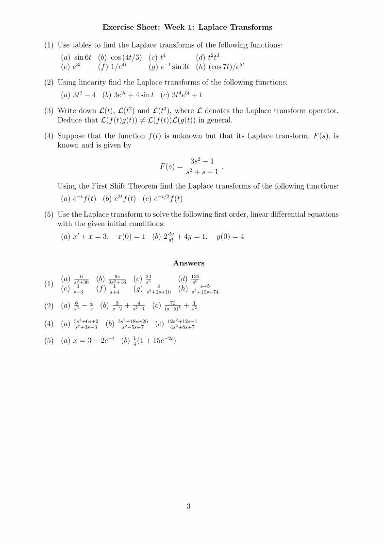
Exercise Sheet: Week 1: Laplace Transforms

(1) Use tables to find the Laplace transforms of the following functions:

(a) sin 6t (b) cos (4t/3) (c) t4 (d) t2t3

(e) e3t (f) 1/e4t (g) e−t sin 3t (h) (cos 7t)/e5t

(2) Using linearity find the Laplace transforms of the following functions:

(a) 3t2 − 4 (b) 3e2t + 4 sin t (c) 3t4e5t + t

(3) Write down L(t), L(t2) and L(t3), where L denotes the Laplace transform operator.Deduce that L(f(t)g(t)) 6= L(f(t))L(g(t)) in general.

(4) Suppose that the function f(t) is unknown but that its Laplace transform, F (s), isknown and is given by

F (s) =3s2 − 1

s2 + s + 1.

Using the First Shift Theorem find the Laplace transforms of the following functions:

(a) e−tf(t) (b) e3tf(t) (c) e−t/2f(t)

(5) Use the Laplace transform to solve the following first order, linear differential equationswith the given initial conditions:

(a) x′ + x = 3, x(0) = 1 (b) 2dydt

+ 4y = 1, y(0) = 4

Answers

(1)(a) 6

s2+36(b) 9s

9s2+16(c) 24

s5 (d) 120s6

(e) 1s−3

(f) 1s+4

(g) 3s2+2s+10

(h) s+5s2+10s+74

(2) (a) 6s3 − 4

s(b) 3

s−2+ 4

s2+1(c) 72

(s−5)5+ 1

s2

(4) (a) 3s2+6s+2s2+3s+3

(b) 3s2−18s+26s2−5s+7

(c) 12s2+12s−14s2+8s+7

(5) (a) x = 3− 2e−t (b) 14(1 + 15e−2t)

3

Week 2: Inverse Laplace transforms

Learning outcomes. You should be able to:

(i) Write down the inverse Laplace transforms of some standard functions.

(ii) Compute the inverse L.T. using partial fractions.

(iii) Compute the inverse L.T. by completing the square.

Reading: Lecture notes plus handout on Laplace Transforms,CDH pages 516–520.

Exercises: Handbook exercise sheet:Week2: Inverse Laplace tranforms

4

Exercise Sheet: Week 2: Inverse Laplace Transforms

(1) Use tables to find the inverse Laplace transforms of:

(a)1

s(b)

2

s3(c)

8

s(d)

6

s + 4

(e)5

s− 3(f)

2

s2 + 4(g)

s

s2 + 9(h)

20

s2 + 16

(i)2

(s + 1)2(j)

9

(s + 3)3

(2) Using linearity (and some ingenuity!) find the inverse Laplace transforms of:

(a)3

2s(b)

4

s− 1

s3(c)

30

s2(d)

1

3(s + 2)

(e)3s− 7

s2 + 9(f)

s + 4

(s + 4)2 + 1(g)

5

(s + 4)2 + 1(h)

6s + 17

(s + 4)2 + 1

(i)s + 5

s2 + 8s + 20(j)

6s + 9

s2 + 2s + 10(k)

7s + 3

s2 + 4s + 8

(3) Use partial fractions to find the inverse Laplace transforms of:

(a)5s + 2

(s + 1)(s + 2)(b)

4s + 1

s(s + 2)(s + 3)(c)

3s + 5

(s + 1)(s2 + 3s + 2)

(d)2s− 8

(s + 2)(s2 + 7s + 6)(e)

s2 + 4s + 4

s3 + 2s2 + 5s(f)

1− s

(s + 1)(s2 + 2s + 2)

(g)s + 4

s2 + 4s + 4(h)

3s2 − s + 8

(s + 2)(s2 − 2s + 3)

Answers

(1)(a) 1 (b) t2 (c) 8 (d) 6e−4t

(e) 5e3t (f) sin 2t (g) cos 3t (h) 5 sin 4t(i) 2te−t (j) (9/2)t2e−3t

(2)(a) 3/2 (b) 4− t2/2 (c) 30t (d) e−2t/3(e) 3 cos 3t− (7/3) sin 3t (f) e−4t cos t (g) 5e−4t sin t

(h) 6e−4t cos t− 7e−4t sin t (i) e−4t cos 2t + (1/2)e−4t sin 2t(j) 6e−t cos 3t + e−t sin 3t (k) 7e−2t cos 2t− (11/2)e−2t sin 2t

(3)

(a) 8e−2t − 3e−t (b) 1/6 + (7/2)e−2t − (11/3)e−3t

(c) e−t + 2te−t − e−2t (d) 3e−2t − e−6t − 2e−t

(e) 1/5(4 + e−t cos 2t + (11/2)e−t sin 2t) (f) e−t(2− 2 cos t− sin t)

(g) e−2t(1 + 2t) (h) e−t(cos√

2t +√

2 sin√

2t) + 2e−2t

5

Week 3: Laplace Transforms and Ordinary Differential Equations

Learning outcomes. You should be able to:

(i) compute the Laplace transform of first and second derivatives,

(ii) solve linear, second order differential equations via Laplace transforms.

Reading: Lecture notes plus Laplace transforms handoutCDH pages 515, 526–533

Exercises: Handbook exercise sheet:Week 3: Laplace transforms and differential equations

6

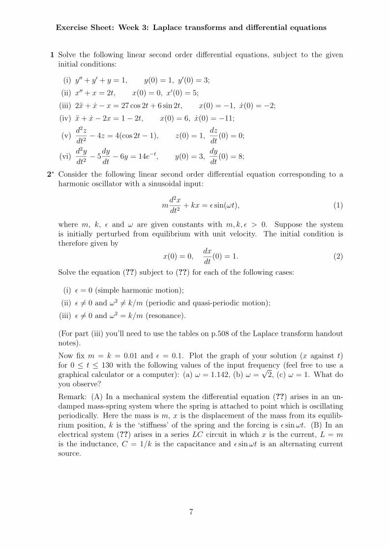
Exercise Sheet: Week 3: Laplace transforms and differential equations

1 Solve the following linear second order differential equations, subject to the giveninitial conditions:

(i) y′′ + y′ + y = 1, y(0) = 1, y′(0) = 3;

(ii) x′′ + x = 2t, x(0) = 0, x′(0) = 5;

(iii) 2x + x− x = 27 cos 2t + 6 sin 2t, x(0) = −1, x(0) = −2;

(iv) x + x− 2x = 1− 2t, x(0) = 6, x(0) = −11;

(v)d2z

dt2− 4z = 4(cos 2t− 1), z(0) = 1,

dz

dt(0) = 0;

(vi)d2y

dt2− 5

dy

dt− 6y = 14e−t, y(0) = 3,

dy

dt(0) = 8;

2∗ Consider the following linear second order differential equation corresponding to aharmonic oscillator with a sinusoidal input:

md2x

dt2+ kx = ε sin(ωt), (1)

where m, k, ε and ω are given constants with m, k, ε > 0. Suppose the systemis initially perturbed from equilibrium with unit velocity. The initial condition istherefore given by

x(0) = 0,dx

dt(0) = 1. (2)

Solve the equation (??) subject to (??) for each of the following cases:

(i) ε = 0 (simple harmonic motion);

(ii) ε 6= 0 and ω2 6= k/m (periodic and quasi-periodic motion);

(iii) ε 6= 0 and ω2 = k/m (resonance).

(For part (iii) you’ll need to use the tables on p.508 of the Laplace transform handoutnotes).

Now fix m = k = 0.01 and ε = 0.1. Plot the graph of your solution (x against t)for 0 ≤ t ≤ 130 with the following values of the input frequency (feel free to use agraphical calculator or a computer): (a) ω = 1.142, (b) ω =

√2, (c) ω = 1. What do

you observe?

Remark: (A) In a mechanical system the differential equation (??) arises in an un-damped mass-spring system where the spring is attached to point which is oscillatingperiodically. Here the mass is m, x is the displacement of the mass from its equilib-rium position, k is the ‘stiffness’ of the spring and the forcing is ε sin ωt. (B) In anelectrical system (??) arises in a series LC circuit in which x is the current, L = mis the inductance, C = 1/k is the capacitance and ε sin ωt is an alternating currentsource.

7

Answers

1 (i) y = 1 + 2√

3e−t/2 sin (√

3t/2);

(ii) x = 3 sin t + 2t;

(iii) x = −3 cos 2t + 2e−t;

(iv) x = t + 6e−2t;

(v) z = (1/4)e−2t + (1/4)e2t − (1/2) cos 2t + 1;

(vi) y = (8/7)e−t + (13/7)e6t − 2te−t;

2 (i) x = (1/ω0) sin ω0t, where ω20 = k/m;

(ii) x =

[ω2

0 − ω2 − (ε/m)ω

ω0(ω20 − ω2)

]sin ω0t +

[ε/m

ω20 − ω2

]sin ωt;

(iii) x =

[2ω0 + (ε/m)

2ω20

]sin ω0t−

[(ε/m)

2ω0

]t cos ω0t.

8

Weeks 4-6: Vector geometry of lines, planes and curves

Introduction: Certain physical quantities are fully described by a single number or scalar,e.g. mass, speed. Other quantities are not fully decribed unless a direction is specified inaddition to a scalar. e.g. electric field, pressure, velocity. Such quantities are called vectors.Vectors are a very useful way to describe positions and orientations in space. In particular,we will use them to describe the geometry of lines, planes and curves in three-dimensionalspace and to investigate some simple problems in particle motion.

Week 4: Vector geometry of planes

Learning outcomes. You should be able to:

(i) Define and compute the vector equation of a plane.

(ii) Define and compute the Cartesian equation of a plane.

(iii) Calculate the anlge between two planes.

(iv) Calculate the distance of a point from a plane.

Reading: Lecture notes

Exercises: Handbook exercise sheet:Week 4: Vector geometry of planes.

9

Exercise Sheet: Week 4: Vector geometry of planes

1 The following planes have been expressed in Cartesian form. Rewrite them in vectorform:

(i) 2x− 3y + 4z = −1 (ii) y = 0

2 The following planes have been expressed in vector form. Rewrite them in Cartesianform:

(i) r · (2i + j− 3k) = 3 (ii) r · (−j + 2k) = 0

3 Find the Cartesian equation of the plane passing through the three points P =(−4,−1,−1), Q = (−2, 0, 1) and R = (−1,−2,−3).

4 Determine whether the given point A lies on the given plane P :

(i) P : x + z = 7; A = (12,−4,−5)

(ii) P : −x− y + 4z = 1; A = (1, 0, 1)

5 Determine whether the four points P = (1, 1, 1), Q = (3, 1,−1), R = (0, 1,−7) andS = (2, 1, 3) lie in the same plane (i.e. coplanar).

6 Determine whether the following planes are parallel, perpendicular or neither:

(i) P1 : x− y + 2z = 0; P2 : −3x + 3y − 6z = 7

(ii) P1 : −x− 11y + 2z = 1; P2 : 2x + z = −3

(iii) P1 : 7x + 3y − 4z = −1; P2 : 2x + 2y − z = 0

7 Find the acute angle of intersection between the two planes P1 : 2y − 2z = 1 andP2 : 3x + y − z = 1.

8 Find the distance of the point (3, 1,−2) from the plane x + 2y − 2z = 4.

10

Answers

1 (i) r · (2i− 3j + 4k) = −1

(ii) r · j = 0

2 (i) 2x + y − 3z = 3

(ii) −y + 2z = 0

3 2y − z = −1

4 (i) Yes; (ii) No

5 Coplanar

6 (i) Parallel; (ii) Perpendicular; (iii) Neither

7 64.76 degrees

8 5/3

11

Week 5: Vector geometry of lines

Learning outcomes. You should be able to:

(i) Define and compute the vector equation of a line.

(ii) Define and compute the parametric equation of a line.

(iii) Calculate the angle between two lines.

(iv) Find the intersection point of two lines.

(v) Find the intersection point of a line and a plane.

(vi) Calculate the angle between a line and a plane.

Reading: Lecture notes

Exercises: Handbook exercise sheet:Week 5: Vector geometry of lines.

12

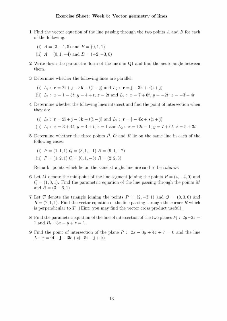
Exercise Sheet: Week 5: Vector geometry of lines

1 Find the vector equation of the line passing through the two points A and B for eachof the following:

(i) A = (3,−1, 5) and B = (0, 1, 1)

(ii) A = (0, 1,−4) and B = (−2,−3, 0)

2 Write down the parametric form of the lines in Q1 and find the acute angle betweenthem.

3 Determine whether the following lines are parallel:

(i) L1 : r = 2i + j− 3k + t(i− j) and L2 : r = j− 3k + s(i + j)

(ii) L1 : x = 1− 3t, y = 4 + t, z = 2t and L2 : x = 7 + 6t, y = −2t, z = −3− 4t

4 Determine whether the following lines intersect and find the point of intersection whenthey do:

(i) L1 : r = 2i + j− 3k + t(i− j) and L2 : r = j− 4k + s(i + j)

(ii) L1 : x = 3 + 4t, y = 4 + t, z = 1 and L2 : x = 12t− 1, y = 7 + 6t, z = 5 + 3t

5 Determine whether the three points P , Q and R lie on the same line in each of thefollowing cases:

(i) P = (1, 1, 1) Q = (3, 1,−1) R = (9, 1,−7)

(ii) P = (1, 2, 1) Q = (0, 1,−3) R = (2, 2, 3)

Remark: points which lie on the same straight line are said to be colinear.

6 Let M denote the mid-point of the line segment joining the points P = (4,−4, 0) andQ = (1, 3, 1). Find the parametric equation of the line passing through the points Mand R = (3,−6, 1).

7 Let T denote the triangle joining the points P = (2,−3, 1) and Q = (0, 3, 0) andR = (2, 1, 1). Find the vector equation of the line passing through the corner R whichis perpendicular to T . (Hint: you may find the vector cross product useful).

8 Find the parametric equation of the line of intersection of the two planes P1 : 2y−2z =1 and P2 : 3x + y + z = 1.

9 Find the point of intersection of the plane P : 2x − 3y + 4z + 7 = 0 and the lineL : r = 9i− j + 3k + t(−5i− j + k).

13

Answers

1 (i) r = 3i− j + 5k + t(3i− 2j + 4k)

(ii) r = j− 4k + t(i + 2j− 2k)

2 (i) x = 3− 3t, y = 2t− 1, z = 5− 4t

(ii) x = t, y = 2t + 1, z = −4− 2t

Angle is 56.1 degrees.

3 (i) Not parallel

(ii) Parallel

4 (i) Don’t intersect

(ii) Intersect at (−17,−1, 1)

5 (i) Colinear

(ii) Not colinear

6 x = 5/2 + t, y = −1/2− 11t, z = 1/2 + t

7 r = 2i + j + k + t(i− 2k)

8 x = t, y = 3(1− 2t)/4, z = (1− 6t)/4

9 (−1733

,−433, 49

3)

14

Week 6: Vector Geometry of Curves

Learning outcomes. You should be able to :

(i) Define the parametric and vector equation of a curve.

(ii) Sketch simple curves (e.g. parabola, circle) given in parametric or vector form.

(iii) Define and compute the first and second derivative of a vector.

(iv) Compute the derivative of a scalar or vector product.

Reading: Lecture notes

Exercises: Handbook exercise sheet:Week 6: Vector Geometry of Curves

15

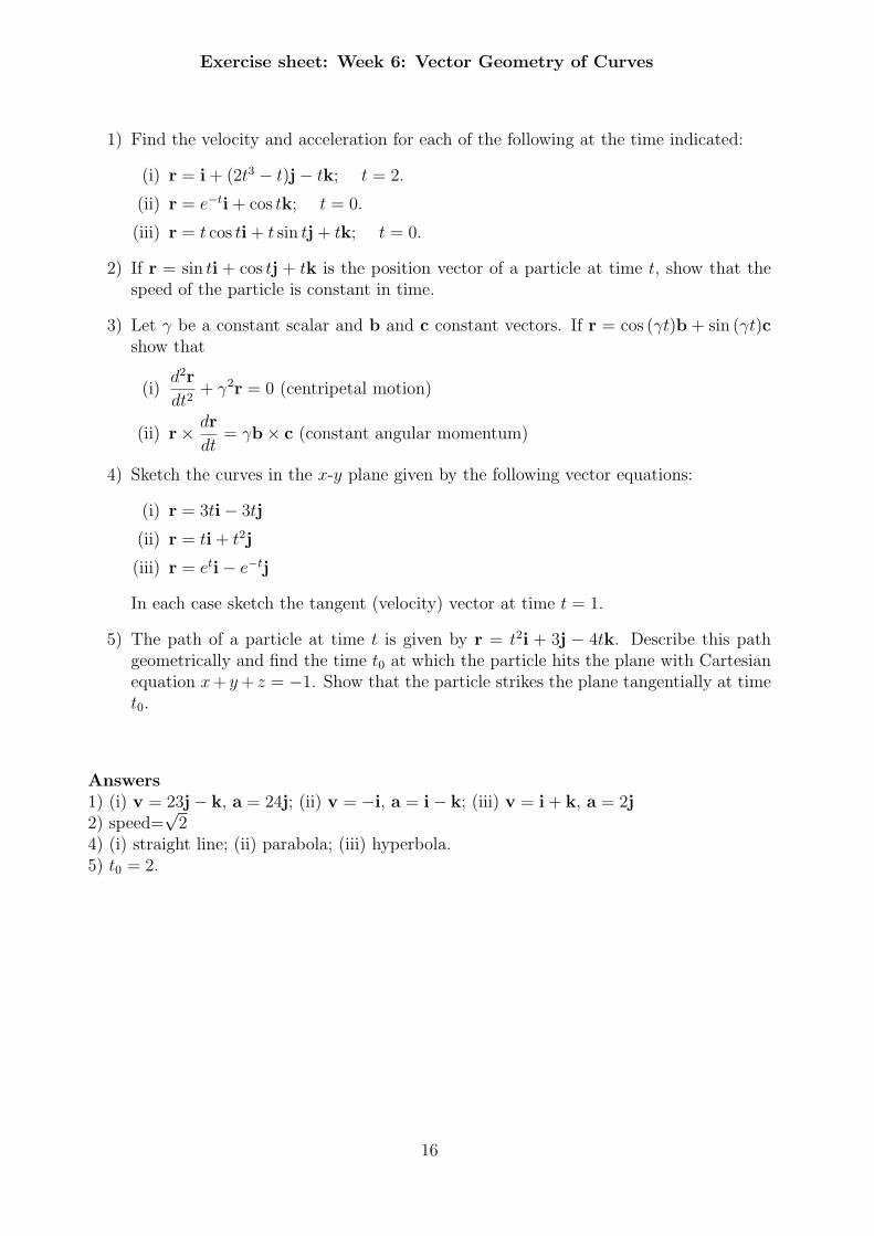
Exercise sheet: Week 6: Vector Geometry of Curves

1) Find the velocity and acceleration for each of the following at the time indicated:

(i) r = i + (2t3 − t)j− tk; t = 2.

(ii) r = e−ti + cos tk; t = 0.

(iii) r = t cos ti + t sin tj + tk; t = 0.

2) If r = sin ti + cos tj + tk is the position vector of a particle at time t, show that thespeed of the particle is constant in time.

3) Let γ be a constant scalar and b and c constant vectors. If r = cos (γt)b + sin (γt)cshow that

(i)d2r

dt2+ γ2r = 0 (centripetal motion)

(ii) r× dr

dt= γb× c (constant angular momentum)

4) Sketch the curves in the x-y plane given by the following vector equations:

(i) r = 3ti− 3tj

(ii) r = ti + t2j

(iii) r = eti− e−tj

In each case sketch the tangent (velocity) vector at time t = 1.

5) The path of a particle at time t is given by r = t2i + 3j − 4tk. Describe this pathgeometrically and find the time t0 at which the particle hits the plane with Cartesianequation x+ y + z = −1. Show that the particle strikes the plane tangentially at timet0.

Answers1) (i) v = 23j− k, a = 24j; (ii) v = −i, a = i− k; (iii) v = i + k, a = 2j2) speed=

√2

4) (i) straight line; (ii) parabola; (iii) hyperbola.5) t0 = 2.

16

Weeks 7-9 Eigenvalues and Eigenvectors

Introduction: Many engineering problems can be formulated as systems of linear differen-tial equations (continuous time) or linear difference equations (discrete time). These can bewritten in matrix form. Associated to any square matrix there are special numbers (eigen-values) and vectors (eigenvectors). The signs or magnitudes of the eigenvalues essentiallydetermine whether the solutions of a given system oscillate, decay to zero or grow unbound-edly as time increases. We will concentrate on the mathematical techniques required tocompute eigenvalues and eigenvectors. Applications to difference and differential equationswill be given in weeks 8 and 9.

Week 7: Introduction to eigenvalues and eigenvectors

Learning outcomes. You should be able to:

(i) Define what is meant by an eigenvalue and an eigenvector of a square matrix.

(ii) Compute the eigenvalues and eigenvectors of 2× 2 and 3× 3 matrices.

Reading: Lecture notes plus handout on ‘Eigenvalues and eigenvectors’pages 189-195 (taken from Mathematical Techniques by Jordan and Smith).

Exercises: Handout, Page 211-213, Problems Qns. 11.1 (a),(b), 11.2, 11.3,11.4 (a),(b),(c), 11.22

17

Week 8: Discrete linear systems

Learning outcomes. You should be able to:

(i) Determine the eigenvalues and eigenvectors of the matrix An.

(ii) Solve systems of linear difference equations.

(iii) Determine whether the solutions of such a system decay to zero, oscillate or growunboundedly over time using only the eigenvalues.

Reading: Lecture notes

Exercises: Handbook exercise sheet:Week 8: Discrete Linear Systems .

18

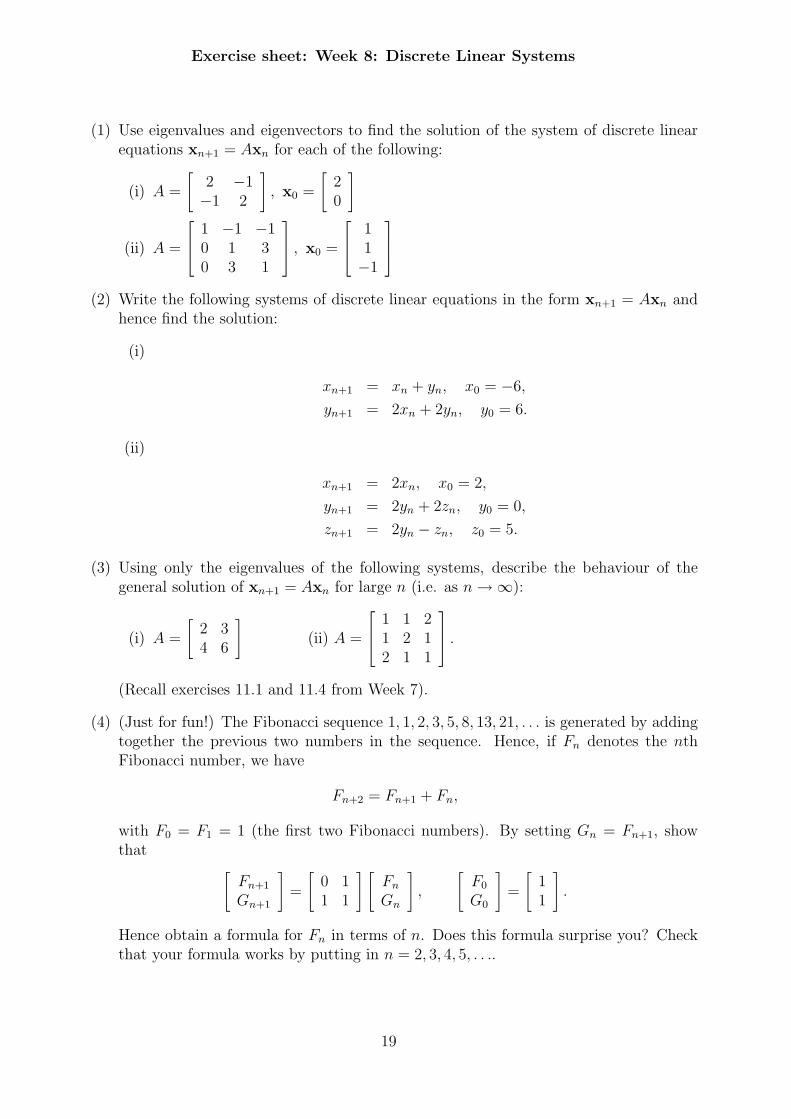
Exercise sheet: Week 8: Discrete Linear Systems

(1) Use eigenvalues and eigenvectors to find the solution of the system of discrete linearequations xn+1 = Axn for each of the following:

(i) A =

[2 −1−1 2

], x0 =

[20

]

(ii) A =

1 −1 −10 1 30 3 1

, x0 =

11−1

(2) Write the following systems of discrete linear equations in the form xn+1 = Axn and

hence find the solution:

(i)

xn+1 = xn + yn, x0 = −6,

yn+1 = 2xn + 2yn, y0 = 6.

(ii)

xn+1 = 2xn, x0 = 2,

yn+1 = 2yn + 2zn, y0 = 0,

zn+1 = 2yn − zn, z0 = 5.

(3) Using only the eigenvalues of the following systems, describe the behaviour of thegeneral solution of xn+1 = Axn for large n (i.e. as n →∞):

(i) A =

[2 34 6

](ii) A =

1 1 21 2 12 1 1

.

(Recall exercises 11.1 and 11.4 from Week 7).

(4) (Just for fun!) The Fibonacci sequence 1, 1, 2, 3, 5, 8, 13, 21, . . . is generated by addingtogether the previous two numbers in the sequence. Hence, if Fn denotes the nthFibonacci number, we have

Fn+2 = Fn+1 + Fn,

with F0 = F1 = 1 (the first two Fibonacci numbers). By setting Gn = Fn+1, showthat [

Fn+1

Gn+1

]=

[0 11 1

] [Fn

Gn

],

[F0

G0

]=

[11

].

Hence obtain a formula for Fn in terms of n. Does this formula surprise you? Checkthat your formula works by putting in n = 2, 3, 4, 5, . . ..

19

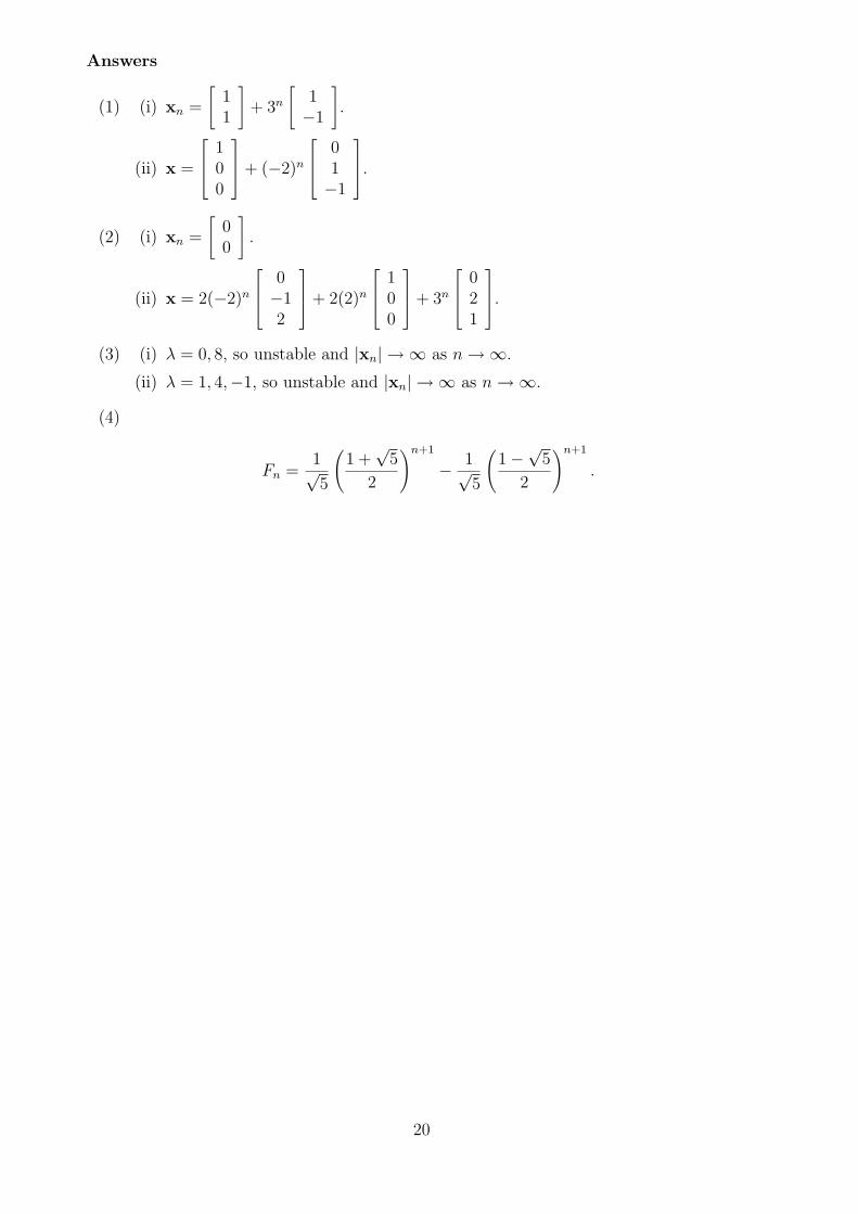
Answers

(1) (i) xn =

[11

]+ 3n

[1−1

].

(ii) x =

100

+ (−2)n

01−1

.

(2) (i) xn =

[00

].

(ii) x = 2(−2)n

0−12

+ 2(2)n

100

+ 3n

021

.(3) (i) λ = 0, 8, so unstable and |xn| → ∞ as n →∞.

(ii) λ = 1, 4,−1, so unstable and |xn| → ∞ as n →∞.

(4)

Fn =1√5

(1 +

√5

2

)n+1

− 1√5

(1−

√5

2

)n+1

.

20

Week 9 Continuous linear systems

We will apply some of the techniques you have learned on eigenvalues, eigenvectors andLaplace transforms to analyse the stability of systems of linear differential equations. Theseideas are central to the qualitiative understanding of dynamical and control systems engi-neering and design.

Learning outcomes. You should be able to :

(i) Define what is meant by ‘stability’ for differential systems.

(ii) Determine when a system of linear differential equations is stable.

Reading: Lecture notes

Exercises: Handbook exercise sheet:Week 9: Continuous linear systems

21

Exercise sheet: Week 9: Continuous linear systems

(1) Use eigenvalues and eigenvectors to find the solution of the system of differentialequations x = Ax, x(0) = x0 for each of the following:

(i) A =

[3 −22 −2

], x0 =

[−11

](ii) A =

[−3 22 −3

], x0 =

[31

]

(iii) A =

1 −1 −10 1 30 3 1

, x0 =

−106

(2) Using only the eigenvalues decide whether the system of differential equations x = Ax

is stable for each of the following:

(i) A =

[−2 11 −3

](ii) A =

[2 −13 −2

]

(iii) A =

[4 2−13 −6

]

(3) Recall the system of differential equations describing a series LCR circuit:

Q = I,

I = − 1

LCQ− R

LI.

Using only the eigenvalues determine the stability of this system in the two cases (i)R2 > 4L/C and (ii) R2 < 4L/C. In each case describe the qualitative behaviour ofthe solutions for large time i.e. as t →∞. A sketch will do!

(4) An unforced, damped oscillator may be described via Hooke’s Law and Newton’sSecond Law by the differential equation

mx + cx + kx = 0.

Here mx is “mass × acceleration”, cx is a frictional force and kx is the tension inthe spring. By letting y = x show that this equation can be written as the system ofdifferential equations

x = y,

y = − k

mx− c

my.

Determine the stability of this system in the two cases (i) c2 > 4mk and (ii) c2 < 4mk.In each case describe the qualitative behaviour of the solutions as t →∞.

22

Answers

(1) (i) x =

[12

]e−t −

[21

]e2t.

(ii) x = 2

[11

]e−t +

[1−1

]e−5t.

(iii) x =

100

et +

−233

e4t + 3

0−11

e−2t.

(2) (i) λ =−5±

√5

2, stable.

(ii) λ = ±1, unstable.

(ii) λ = −1± j, stable.

(3) (i) Eigenvalues real and negative. Hence stable. Solutions decay monotonically tozero.

(ii) Eigenvalues complex with negative real part σ. Hence stable. Solutions oscillateand decay to zero.

(4) (i) Eigenvalues real and negative. Hence stable. Solutions decay monotonically tozero.

(ii) Eigenvalues complex with negative real part σ. Hence stable. Solutions oscillateand decay to zero.

23

Weeks 10-12 Fourier Series

Introduction: The ability to analyse waveforms of various types is an important engineer-ing tool. Fourier analysis provides a mathematical tool which enables the engineer to breakdown a wave or signal into its various frequency components. This is particularly usefulin communications. Fourier series are also a useful mathematical tool for solving partialdifferential equations describing heat flow or electrostatics problems.

Week 10: Introduction to Fourier Series

Learning outcomes. You should be able to:

(i) Determine the period of any given periodic function.

(ii) Sketch a periodic function (continuous and discontinuous).

(iii) Understand what a Fourier series is and how it approximates a given periodic function.

(iv) Compute integrals using integration by parts.

Reading: Lecture notes.

Exercises: Handbook exercise sheet:Week 10: Integration and Periodic Functions.

24

Week 11: More on Fourier Series

Learning outcomes. You should be able to:

(i) Calculate the coefficients an and bn of the Fourier series for any periodic function.

(ii) Sketch the Fourier series for any periodic function.

(iii) Determine the value of a Fourier series for any given argument.

Reading: Lecture notes.

Exercises: Handbook exercise sheet:Week 11: Fourier Series

Week 12 Fourier series/Revision

We will use the final week to complete any outstanding work on Fourier series and, timepermitting, go through some exam-type questions.

25