h. ,

DE-FC22-95PC95051-17

Engineering Development of Slurry Bubble Column Reactor(SBCR) Technology “

Quarterly ReportApril 1- June 39,1996

By:Bernard A. ToseIand

Work Performed Under Contract No.: DE-FC22-95PC95051

ForU.S. Department of Energy

Office of Fossil EnergyFederal Energy Technology Center

P.O. Box 880Morgantowq West Virginia 26507-0880

ByAir Products and Chemicals, Inc.

7201 Hamilton BoulevardAllento~ Pennsylvania 18195-1501

Disclaimer,... .

This report was prepared as an account of work sponsored by anagency of the United States Government. Neither the United StatesGovernment nor any agency thereof, nor any of their employees,makes any warranty, express or implied, or assumes any legal liabilityor respondility for the accuracy, completeness, or usefulness of anyinformation, apparatus, product, or process disclosed, or representsthat its use would not intiinge privately owed rights. Reference-hereinto any specificconynercial product, process, or service by trade name,trademark manufacturer, or otherwise does not necessarily constituteor impIyits endorsement, recommendation, or favoring by the UnitedStates Government or any agency thereof. The views and opinions ofauthors expressed here~ndo not necessarily state or reflect those ofthe United States Government or any agency thereof.

DISCLAIMER

Portions of this document may be illegiblein electronic image products. Images areproduced from the best available originaldocument.

ENGINEERING DEVELOPMENT OF SLURRY BUBBLE COLUMN REACTOR(SBCR) TECHOLOGY

Quarterly Technical Progress Report No. 5for the Period 1 April -30 June 1996

Contract ObjectivesThe major technical objectives of this program are threefold: 1) to develop the designtools and a fundamental understanding of the fluid dynamics of a slurry bubble columnreactor to maximize reactor productivity, 2) to develop the mathematical reactor designmodels and gain an understanding of the hydrodynamic fimdarnentals under industriallyrelevant process conditions, and 3) to develop an understanding of the hydrodynamics andtheir interactionwiththechemistriesoccurringin thebubblecolumnreactor. Successfulcompletion of these objectives will permit more efficient usage of the reactor column andtighter design criteria, increase overall reactor efficiency, and ensure a design that leads tostable reactor behavior when scaling up to large diameter reactors.

Summary of Progress

● State of the ArtAssessment of tomography and densitometry has been completed, and a report isunder review. A “poor man’s tomograph” suitable for installation at LaPorte has beendesigned, details will be published in a topical repot which is under second revision.

(Washington University in St. Louis)(Air Products and Chemicals, Inc.)

A search of the literature on spargers provided insight into what parameters should beconsidered in sparger design. However, insufficient information is available forsparger design for industrial systems at high gas flow rates and elevated pressures.Good design methods exist for understanding the generation of bubbles, but designmethods for spargers in columns do not exist. Additional experimental work is neededto begin to understand the importance of various sparger parameters on columnperformance.

(Air Products and Chemicals, Inc.)

Task 2- TechniqueDevelopn~entUnderstanding physical phenomena requires an understanding of the physicalproperties of the system understudy. Because the effect of high temperature and -pressure on viscosity is very difficult to predict, measurements are needed. A fallingball viscometer was devised for the high-pressure/high-temperature column, and itsoperation was validated at low pressure. Viscosity of liquids at high temperature andpressure was measured. The complicated effect of temperature at high pressure wasdemonstrated; as pressure increased from 0.1 to 21 MPa, the viscosity increased by65% at 20°C and by only 10% at 100°C.

(The Ohio State University)

Task 3- Model Development -A new phenomenological model was developed for the liquid and gas phase in abubble column reactor. It employs the same concept--recirculating cell withinterchange coefficients--as the liquid phase model described in previous reports. Thegas phase is described by a two-bubble class model. The large bubbles rise with highvelocity in plug flow in the core region of the bubble column, while the small bubblesmove more slowly in both upflow in the core and downflow, carried by the liquid, inthe wall region. Interchange is aIlowed between bubble classes so that coalescenceand breakup of the bubbles can be described.

(Washington University in St.Louis)

Task 4- SBCR Ekperi-numtal Program

Transient flow fields in a 2D air-water bubble column were measured using the PIVtechnique. Velocity profiles and Reynolds stresses were obtained. Since the Reynoldsshear stress is proportional to the averaged vertical velocity gradien~ these data verifythe Boussinesqu hypothesis. However, the Reynold’s normal stresses are much greaterthan the shear stresses. This finding challenges “theusual symmetry of stressassumptions made in CFD calculations.

(The Ohio State University)

Time series analysis of the 2D column data shows the presence of vortices in the flowfield. Several characteristic frequencies are revealed by the power spectrum analysis,but high-frequency signals are low, indicating that the vortex structure is the mainfeature of the flow, and other “purely turbulent” energy contributions are rather low.

(The Ohio State University)

The effect of pressure on gas holdup was measured for gas flow rates up to 8 cm/sec.Gas holdup increases with increasing pressure up to about 10 MPa. Because theaverage bubble size was insensitive to pressure, the increase in holdup must be due alarger number of bubbles at high pressure.

(The Ohio State University)

Task 6-Data ProcessingThe liquid recirculation with crossflow and dispersion model (RCFD) matched, at leastsemi-quantitatively, the tracer test results obtained during the last test at the AFDU inLaPorte. Since this model had no adjustable parameters (model parameters wereestimated from laboratory data), the agreement is noteworthy.

(Washington University in St. Louis)

.

.. .

The Ohio State University Research

The following report from Ohio State University for the period April - June 1996 containsthe following brief chapters:

1. Measurement of liquid viscosity (Task 2-5)2. Bubble effects on the transient flow pattern in bubble columns (Task 3)3. Gas holdup in high-pressure and -temperature bubble column (Task 4)4. Work to be-performed next quarter (Task 7)5. References

●

✎✌✎ ✌

INTRINSIC FLOW BEHAVIOR IN A SLURRY BUBBLE

COLUMNUNDERHIGH PRESSUREAND HIGH TEMPERATURE CONDITIONS

(Quarterly Report)

(Reporting Period: April 1 to June 30, 1996)

Liang-Shih Fan

DEPARTMENT OF CHEMICAL ENGINEERINGTHE OHIO STATE UNIVERSITY

COLUMBUS, OHIO 43210

July 17, 1996

Prepared for Air Products and Chemicals, Inc...-

WORK PERFORMED

1. Measurement of liquid viscosi@

The experiments on liquid viscosity measurement were started two months ago. The .

experiments were conducted in the high pressure and temperature system, and nitrogen was used

to pressurize the system. The molecular structures of Paratherm NF heat tmnsfer fluid and other

oganic liquid (e.g, mineral oil and F-T wax) are complex. There is no theoretical method to

accurately estimate the viscosity of these liquid. Thus, direct measurements using such methods

as falling ball and plate-and-cone or couette-type viscometers are the only alternative. In the

d~ect measurement of liquid viscosity conducted in thii study, falling ball technique was used to

measure the viscosity of Paratherm NF heat transfer fluid. The Reynolds number based on the

particle diameter is maintained in all experiments at less than 2 by varying the particle sizes. The

Stokes (1851) and Oseen (1910) equations given below were applied to calculate the viscosity for

different flow regimes, based on the Reynolds number:

d;(PP -p>gAtP ‘f. (Re,<O.1)

18L

d;(pp - p)@P ‘fw (0.l<Re:2)

18L (1 +3Re#6)

(1)

(2)

where~Wisthe cmrection factor accounting for the wall efkct, and can be expressed by (Khan and

Richardson, 1989)

fw = 1- 1.15(dp/D)006 (3)

.

Figure 1 shows the variations of the viscosity with pressure and temperature for Paratherm

NF heat transfer fluid. The results were partially verified by comparing the measurements with

valu~ provided by the Paratherm supplier at a pressure of 0.1 MPa and temperatures below the

boilhg point. The differences between the measured values and the supplier’s results are less than

1%.

1. . .

.. ..

:.,. ,. ‘.. ”. . .. . . “,:. . ,,..— . . . . . . . .. _-.’-

. .

In general, the liquid molecules move within parallel liquid layers, where they change their

sites by surpassing the activation energy barrier (Ewell and Eyring, 1937). As the pressure

increases at low temperatures, the liquid exerts a larger frictional drag on adjacent molecule

layers, and the velocity gradient decreases, which &uses the viscosity to increase signifkantly. ,

For high temperatures, however, the liquid molecules have excess free energy to overcome the

energy barrier, and thus an increase in pressure does not significantly affect the liquid viscosity.

Figure 1 shows that when the pressure increases from 0.1 to 21 MPa, the viscosity for Paratherm

NF heat transfer fluid increases by 65% at 20°C, but only by 10% at 100”C. Figure 1 also

indicates that the effect of temperature on the liquid viscosity is more significant than that of

pressure.

2. Bubble effects on the transient flowpattern in bubble columns

For the flow in a two-dimensional (2-D) air-water bubble column of 15 cm in width at the

supefflckd gas velocity of 1 cm/s, a time series of 322 consecutive vector fields was constructed by

a Particle Image Velocimetry (MY). The PIV technique has the capabildy to provide the transient

IM1-fieldbehavior of a fluid flow ~thout obstructing the flow. The series comprises 10.73 s of the

flow and contains the passage of two vortices in the field of view. This analysis allows for the study

of the flow dynamics in great detail (deterministic and stochastic properties). The profiles of the

averaged horizontal and vertical liqyid velocities, u and v, respectively; and Reynolds stresses were

obtained from the liquid velocity fields as shown in Figures 2 and 3. The averaged vertical liquid

flow consists of upward flow in the center of the column and downward flow adjacent to the

sidewalls. The Reynolds normal stress in the horizontal direction peaks in the center, whereas the

vertical normal stress has a local minimum in the center and maximum between the wall and the... “

cen~r. The Reynolds shear stress is proportional to the gradient of averaged vertical velocity profile

suggesting a Boussinesq type of approximation. Furthermore, the Reynolds normal stresses are

considerably greater than the Reynolds shear stress.

For each field, the liquid vectors were redistributed over a 10 by 10 grid. After the cell

averaged velocities were computed for the entire 10.73 s series, they were subtracted from the

2-.. .

instantaneous vectors in the respective cells. h Figures 4a and 4b, the series of both components

for grid cell (3,5) are shown. It should be noted that the lefl lower cell within the field of view has

coordinates (1, 1). The vertical structures are clearly demonstrated, i.e. periods of positive and

negative axial velocity alternate. Plots for the other grid cells look similar, with the exception of

the cells adjacent to the wails where the horizontal velocity fluctuations are strongly damped and

the center cells where the presence of the vortices is less dominant in the vertical velocity. Figure

5 shows the power spectral density fimctions of both u and v for grid cell (3,5). Agah+ the vertical

structures dominate, i.e. hardly any power is found above1Hz evenup to the Nyquistfrequency

of 15 HZ.

Cross-correlating of u-u for the cells on a horizontal row, i.e. with the samej-coordinate,

reveals that the u-components are in phase. The cross-correlation indicates that the vortices span

the entire column width and flow as one big entity into the field of view. Similarly, cross-

correlating of v-v for a row shows that correlating of two cells at the same side of the column

symmetry axis means zero-phase shift and at different sides gives 180”-phase shift. In the latter

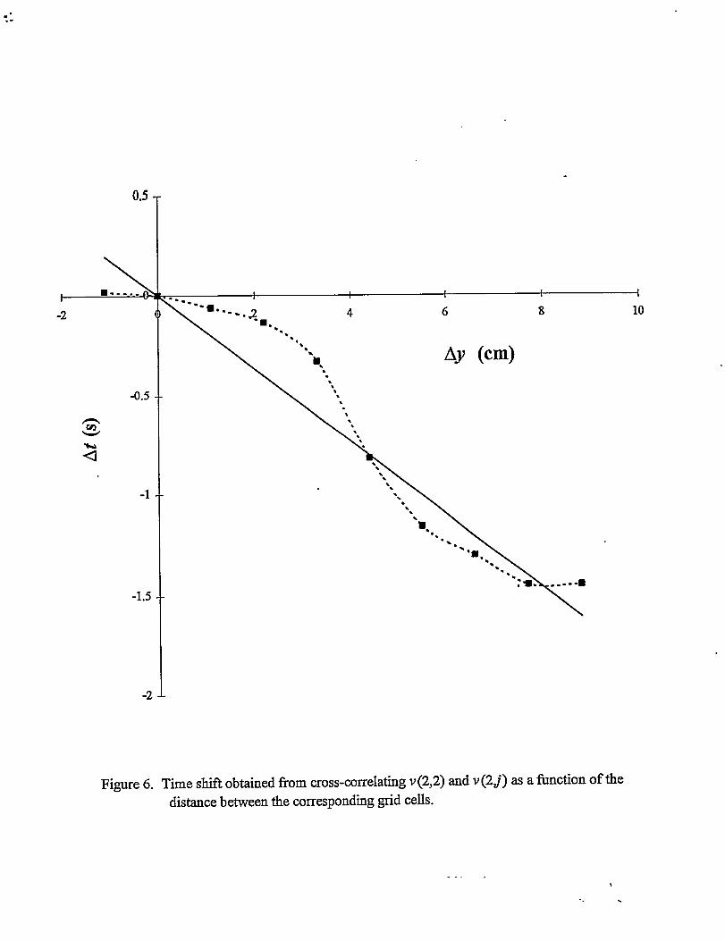
case different sides of the vortex were probed. Finally, from the cross-correlation between v(2,2)

and v(2J) withj = 1 to 10, a time shif$ At, was found to increase with increasing distance, Ay,

between the cells. In Figure 6 this time shift is plotted as a fimction of distance. Fitting a straight

line through the data points gives a reasonable estimate of the descending velocity of the vertical

structures. Note that the negative time shift means cell (2,2) responds later than cell (2~). The

descending velocity of -5.5 crnk was found which shows the vertical structures are moving

downward.

Thedatafromthe time seriesdemonstratethat the velocityfield canbe decomposedinto a

SIOWsine-like oscillation due to the passage of a vortex and ‘high’ fkquency content associated with

‘turbulence’ as shown in Figures 4a and 4b. The power spectra support the use of only one sine-

like carrier wave for the vortices with a fkquency around 0.2 Hz. As mentioned, the flow field can

‘ be decomposed according to:

v(i~”,t) =<v(iJ)> +avcos (27CJ7+qv)+v~(i~-, t) (4)

3

%

..

. .

where v(ij;t) is the vertical component of the velocity in grid cell (ij); <v(i~~>is its time-average;

afl,~ and ~, are the amplitude, frequency and phase to be fitted, respectively; and v~ij;t) is the●

‘turbulent’ part in grid cell (iJ). Now the Reynolds stresses can be recalculated using vps

<v>(iJ)v>(iJ)> =[ )~~ ‘~(iJ@’’iJ,k) ~“ . -

-<v 1J)>2 (5)

The horizontal component of the velocity, q and the oi.hertwo stresses were treated similarly. The

resultant stresses are shown in Figure 7. The figure shows the profiles for one grid row ofj = 5.

The figure demonstrates that removing the contribution of the vortices has a significant affect on

the stresses. With the removal of the vertical structures, relatively flat normal stresses were obtained

that have values close to the minimum in <v’v’>. It can be concluded from this analysis, that the

high frequency content of the normal stresses, i.e. the ‘turbulence’, has a rather flat profile with a

magnitude of 50-100 cm2/s2.

3. Gas Itokkp in high pressure and temperature bubble column

The measurements of gas holdup in the high pressure and temperature bubble column with

a porous plate d~tributor was carried outlast quarter. The experiments were focused on the pressure

effects under various gas velocities. Figure 8 shows the effect of pressure on the gas holdup in the

liquid-batch bubble column. The value of the gas holdup is associated with the bubble rise

velocity and the number density of bubbles in the system. The bubble rise velocity, in turn,

depends on the bubble size and shape, physical properties of the liquid, and flow pattern. In

Figure8, thegasholdupisplottedagainstthe superficialgasvelocityfor pressuresvarying from

0.1 to 20.4 MPa. It is seen that at low gas velocities, the gas holdup increases linearly with

increasing gas velocity for all pressures. The significant pressure effects on the gas holdup were

observed at ~gh gas velocity conditions for pressures up to 10 M’Pa. At pressures higher than 10

MPa, the gas holdup is insensitive to the operating pressure for the gas velocity range examined

in this study. Pressure effects on the gas holdup were reported also to be significant at high gas

velocities by Idogawa et al. (1986) for a air-water system with pressures up to 5 MPa. The

4-.. .

,.-

increasein the gas holdup with increasing pressure can be attributed to a decrease in bubble size

and an increase in number density of bubbles. Visualization revealed that the increase in the gas

holdup from pressures of 3.5 MPa to 20.5 MPa is due to an increase in the bubble number

concentration since the mean bubbIe size is insensitive to the pressure in the current system. As

noted earlier, there is no significant bubble interaction in the dispersed bubble regime, and thus

the condition for the pressure effects on the gas holdup appears to be concerned with the process

of bubble formation. As the gas velocity increases, bubbles of smaller size are formed with a

higher formation frequency in the higher pressure system (Kling, 1962; Idogawa et al., 1987a),

which results in a higher gas holdup compared to those in the system operated under atmospheric

pressures.

WORK TO BE PERFORMED NEXT QUARTER

1. Quantitative analysis of the transient flow pattern in bubble columns will be continued next

qutier with emphasis on the deterministic flow structure.

2. Gas holdup in the high pressure and temperature bubble column will be continued next

quarter.

Notations

D

dP

f.

,,8

L

P

Re

diameter of column (mm)

diameter of particle (mm)

correction factor for wall effect (-)

gravitational acceleration (m/sz)

falling distance (m)

pressure (MPa)

Reynolds number based on particle diameter P@P/P (-)

5..-

. . ,,..’. .— ————-—— .—. -.,. -,—..-— .,. - -—-. — . II

Re, Reynolds number based on particle diameter p#&/p (-)

Greek letters

P liquid viscosity (kg/nrs)

Pp particle density (kg/m3)

Pf liquid density (kg/m3)

REFERENCES

Ewell, R.H. and H. Eyring, “Theory of the Viscosity of Liquids as a Function of Temperature

and Pressure, ” .T. Chem. Phys., 5, 726 (1937).

Idogaw~ K., K. Iked~ T. Fukud~ and S. Morook~ S., “Behavior of bubbles of air-water system

in a column under high pressure,” Inter. Chenz. Eng., 26,468 (1986).

Idogaw~ K, K. llced~ and T. Fukud~ “Formation and flow of gas bubbles in a pressurized bubble

column with a single ofike or nozzle gas distributor,” Clzem. Eng. Comm., 59,201 (1987a).

Khan, A.R. and J.F. Richardson, “Fluid-Particle Interactions and Flow Characteristics of

Fluidti Beds and Settling Suspensions of Spherical Particles,” Chem. Eng. Comm., 78,

111 (1989).

Kling, G., “~er die Dynamik der Blasenbildung Beim Begasen von Flussigkeiten Unter DrucQ”

Inter. JHeatiWzssTrans$er,5,211 (1962).

Oseen, C.W., “~er die Stokes’sche Formel und iiber eine verwandte Aufgabe in der

Hydrodynamik,n Ark. Mat. Astron. Fys., 6,29 (1910).

Stokes, G. G., “On the effect of internal friction of fluids on the motion of pendulums, n Trans.

Cambridge Phil. Sot., 9, 8 (1851).

... -

.,

o0c1

0.~oo0.

---,

..

10

5

0

-5

-lo

.*)* .-

.● *O*“,‘.

‘o.. O..”’O--- ..‘0....--0.

.. ,.. ,‘. .

●.0’”

L

-1 0-0.5 0.5

2x/w

1

Figure 2. Averaged velocity profiles for the middle section of the 11 cm column at UWP= 1.0 ends.

... .$

..

350

300

250

200

150

100

50

0

-50

.

. ,.....

0“

I--Q--<u’u’>

~ <v’v’>

_,O-.. x—.-. <Zf’v’>

#,

.0”’..,’,

o“

-..●

✍✍✍✍✍

7““.*..

●

✎ 9. ,.. ..

. ,’‘0-””

t

x-----

,2 x -x-+-x‘\

x -x’ ●\I o

x___ ,2 “: ‘x~

%.\‘-x

x- - /_x---

.-1 -0.5 0 0.5 1

2x/w

Figure 3. Profiles of the Reynolds stresses component for the middle section of the 15 cm columnat U~P= 1.0 cids. “

. . .\

.. .-2

30

20

10

0

-1(

-2(

-3(

o 2 4 6 8 10

t (s)

Figure 4a. Time series of the fluctuating component of the horizontal velocity of cell (3,5).

12

.-, .

.“.

.

, .... . .. .. . . . .. .

30

20

10

0

-lo

-20

-30

. —————–-—

0 2 4 6 8 10 12

t (s)

Figure 4b. Time series of the fluctuating component of the vertical velocity of cell (3,5).

. . . .I

.

,. .-“. ,’ .,, ” .- “ ,,. :... ,, ..-.—— ------- ——— ... ----. —....–....

25(JUU

6000

4000

2000

(

o

— V(3,5) I

;&, *.

o

: ‘* a:.[[,

:,.I

:8..9

#

.

*,,

s A*e

:

:

s.a, *,, ,et,

[

1

f (Hz)

2 3

Figure 5. Power spectrum of the series shown in Figures 10a and 10b. ,

-.. .

.=,-

0,5

I

t , , , I

-2---9... - , A 6 8 10v

-0.5- -

-1 --

-1.5

-2 1

‘\—.-----8

Figure 6. Time shift obtained from cross-correlating v(2,2) and v(2~) as a fi.mction of thedistance between the corresponding grid cells.

. . . .

,-, . ; ..-.-,.,. . .. . ,.. ,, ...—— —— —— . . ... —.’-....—— —.- ,. :_..- -.. —.. —..= _,. ,

.“.-

300

250

100

50

0

-50

-1

I

~ +lj’up

~ <I.&>

- -A– <Vyvy>

—-A—<Vfv’>

. . G -- <uQ’vy>

. . * -- <Z/v’>

.&. .A

/’

—------lJ- -.

u----- -a. .- 9::-.:. .=---- ----

-0.5 0

2x/w..

0.5

Figure 7. Reynolds stresses for the time series: high frequency fluctuationsand total velocity (closed symbols).

1

(open symbols)

. ... .

‘i

ft I 1 I I I I

2.0 4.0Gas velocity(ads)

6.0 8.0

. .

Figure 8. Eff5cts of gas velocity on the gas holdupat various pressures (T = 25 ‘C).

. . . .

Washington University in St. Louis Research

The following report (which has been submitted as a topical report) from WashingtonUniversity for the period April - June 1996 contains the following chapters:

1. Objectives2. summary3. Appendix A Two Phase Recycle with Cross Flow Model (TRCFM) for Gas Phase in

Bubble Column Reactors (Task 3)4. Appendix B: Progress in Understanding the Fluid Dynamics of Bubble Column

Reactors (Task 6)

. . .

2QTR95.doc

,,

Slurry Bubble Cohmn HydrodynamicsFifth Quarterly Report for Contract DOE-F(7 2295

. June 199~

Subcontract Objectives

Pc 95051

This is thesecondyearof thefiveyearsubcontractfromtheDepartmentof Energyvia Air Products. The main goal of this subcont.met to the Chemical RczictionEngineering

Laboratory (CREL) at Washington University is to study the fluid dynamics of sluny

bubble columns and address issues related to scale-up. All the targets set for&e first year

including

1) review and recommendations of measurement techniques for multiphase flows with

emphasis on the AFDU LaPorte reactor,

2) interpretation of the tracer studies from AFDU I&orte reactor during methanol

synthesis based on the axial dispersion model,

3) modifications of the CA~/CT facility to accommodate studies in slurry systems,

4) development of a phenomenological model for liquid recirculation and

5) testing of closure schemes in CFD modeling) .

have been met in a timely fashion. Two topical reports were submitted to Air Products:

one on measurement techniques in multiphase flows, the other on interpretation of tracer

studies in IaPorte AFDU during methanol synthesis based on the axial dispmion model.

F&the second year of the contract the following objectives are se~

1. Completereviewof gammamytomographyanddensitometryfor obtainingdensity profiles with emphasis on applications in the LaPorte AFDU reactor.

2. Develop phenomenological models for liquid (slurry) and gas flow and

mixing...

3. Use developed phenomenological models in interpretation of tracer runs at

LaPorte.

4. Extend the CARPT/CT database.

5. Continue the ewduation of closure schemes for CFD modeling.

It should be noted that objectives 4 and 5 are really coupled, and may have been

previously reported as a single item, in.mmuch that CARIT/CT data at different conditions

is needed for evaluation of CFD codes.

We will now address progress made in accomplishing the above objectives and in “

summary present a PERT chart as to where we currently stand.

. . .

1

,. ,.,,— ... —- —- —.. . . . . . .. . .. —-.. .

1. ~omowauhy

Evaluationof relativemeritsof tomogmphyanddensitomehyhasbeencompleted.The final topical report on this subject is in preparation and will be issued during the next

quarter. It will contain information relevant to the AFDU hPorte unit.

2. Development of Plte?loljlerzolopical Models for Lianid and Gas Flow

and M ixing

A. Liauid

This model and its governing equations were presented in our3rd quarterly

report and will not be repeated here. The model is based on the experimen-

tally observed steady single cell liquid recirculation pattern. It assumes that

the upflow and downflow liquid stream communicate via an

exchange coefficient (the physical basis for this is the turbulence created

by bubble wakes). In addition, there is axial dispmion in each liquid

region caused by wakes of smaIl bubbles.

B. _Gas

The gas phase model is developed based on the same physical picture

as the liquid model and is described in detail in Appendix A of this report.

3. Use of Phenomenological Models in Interpretation of Tracer Rnns

The liquid recirculation will crossflow and dispemion model (RCFD) outlined in the

3rd quarterly report was set up to predict tracer responses in the AFDU during methanol

synthesis. The model and the methodology used are described in the enclosed paper

prepared for the DOE Joint Power and Fuels Conference in Pittsburgh, July 19% (see

Appendix B). Additional details will be forthcoming in the follow-up reports.

4. Extension of CA RPTICT Data Base bWork continues, as mentioned in monthly reports, to provide data in a larger

diameter 18” column. Results will k discussed in a subsequent reports.

5. Ewdnation of Closnre Schemes for CFD Modeling

This computational effort continues. Comprehensive results will be reported upon

completion of the study.

. ..-

2

SUM MARY

The chart below summarizes the objectives set for the 2nd year of the subcontract andillustrates where we are after the completion of the first quarter of year 2 (fifth quarterovemll).

1. Yomowa hpv

04/01/96 06/30/96 09/30/96 12/31/96 03/31/97

I2. Phenonz enolo~ical Models

2a. Liquid

04/01/96 06/30/96 09/30/96 12/31/96 03/31/97

I

2b. Gas

04/01/96 06/30/96 09/30/96 12/31/96 03/31/97/Zzz I I

3. YSe Of deve~oued !fleno~rleno~o~ cal wi odels in tracer dnta (LaPortel~nterpretation

04/01/96 06/30/96 09/30/96 12/31/96 03/31/97

I I I

4. Extension of CA RPTICT Data Base .

04/01/96 06/30/96 09/30/96 12/31/96 03/31/97

I I I

S. Evaluation o_f CFD M odelx

04/01/96 06/30/96 09/30/96 12/31/96 03/31/97

I I 1

. . .

., . .,,—.-.—. ... . . —. — .—_. . . ...- —...— . . . ..-– .-. ——..—

APPENDIXA

A TWO PHASE RECYCLE WITH CROSS FLOW MODEL (TRCFMI FOR GAS PHASEIN BUBBLE COLUMN REACTORS

Introduction

The ultimate goal in bubble cohmm research is to rapidly scale up from the laborato~ sizeto pilot plant size and finally to industria! bubble column scaIe. It is known that gas andliquid phase mixing, turbulent intensity and residence time distributions are critical to thedesign, scale-up and operation. During the past two decades, modeling of the mixingbehavior of both gas and liquid phases has been widely investigated but it is not yetcompletely successful. This is due to difficulties in describing the complexities of the liquidbackrnixing behavior, including chaotic phenomena and bubble size distribution in the chumturbulent regime either through experiments or via a theoretical approach. The difference inthe behavior of large and small bubbles, the interaction among bubbles in chum turbulentregime due to coalescence and break-up of bubbles, and the coupling of the interphase masstransfer with chemical reactions also make predictive modeling very difficult.

Recently, interest has arisen in operating the bubble column reactors at very high gassupetilcial velocities, ~, in the chum-turbulent regime. In the chum turbulent regime, abimodal bubble size distribution was assumed for the gas phase by Vermeer and Krishna

(1981) and Shah and Joseph (1985). The flow in that regime becomes chaotic, and ischaracterized by fast moving large bubbles in the presence of small bubbles which are carriedwith the recirculated liquid. Gas phase mixing, which is an important hydrodynamicparameter to be considered in the scale-up of bubble columns, cannot be simply modeled bythe axial dispersion model (ADM) in chum turbulent flow. Therefore, a newphenomenological model that relies on the realistic physical picture of bubble cohmms in thechum turbulent regime, and can fit the observed experimental residence time distribution(R’I’D)curves needs to be developed.

A single phase recycle with cross flow model ( RCFM) was first developed in 1970 byHochman and McCord and was successfully applied for tall tanks with a number of axialimpellers. Myers et al (1986) and Degaleesan et al (1996) extended its application bysuccessfidly implementing the model to the liquid phase in bubble column reactors. Fromentand Bischoff (1990) have also noted the applicability of this model to the bubble columnsystem. Based on these findings, a recycle with cross flow type phenomenological model isproposed for both phases in the bubble column in this work. The model parameters aredetermined through experimental observations and empirical correlations.

Model Development.

Based on the experimental observations of Hill (1974) and Devanathan et al (1990), largescale liquid circulation exists in bubble columns. The liquid ascends in the core region of the

. ..-

4 .

column and descends in the annular region close to the wall, which results in the overallliquid circulation and forms what is called a “cell pattern”. Jn the homogeneous regime, e.g.bubbly flow regime, only small bubbles of uniform size exist. These small bubbles, whichare carried with the recirculated liquid, exhibit a slip velocity between the gas and the liquid.The motion of small bubbles in the bubbly flow regime may exhibit two distinct flowpatterns. Small bubbles may rise in the core of the column or descend in the annular regionclose to the wall due to the downward velocity of liquid. Hence, gas recirculation is inducedby liquid circulation, and there is interaction between the upflow of the liquid and thedownflow of the liquid and between the upflow of the small bubbles and downflow of thesmall bubbles due to the shear stress between these two regions.

Theheterogeneousregime,wherethesuperfkialg~ velocityishighenoughsothatthereis adistinct bimodal bubble size distribution, is usually called the ‘chum turbulent regime’. Inthis regime, because of bubble coalescence and break-up, there is interaction not onlybetween the bubbles of the same size but also among bubbles of different sizes. Due to theextreme complexities of bubble interaction and uncertainties regarding the bubble sizedistribution, two bubble sizes (large and small bubbles) are assumed here. Bm,ed onexperimental observations, the large bubbles are assumed to rise in plug flow near the coreregion of the bubble column with higher velocity the small bubbles, which are carried by therecirculated liquid, travel with lower velocity. The recirculation pattern of the smd.11bubblesconsists of upflow in the core region and downflow in the annular region. Figure I shows thetypical flow diagram for small bubbles and liquid, the volume occupied by small bubbles,and the time averaged liquid velocity distribution in each region. Due to the shear betweenthe upflow and the downflow of small bubbles and the liquid itself, it is assumed thatinteractions exist between the small bubbles in the two flow regions, as well as between theliquid in the two flow regions. These interactions are described via exchange coefficients. Inaddition, the exchange coefficient between the small and large bubbles is also defined in themodel. This allows for the coalescence and break-up of the bubbles to be accounted for.

The proposed model may also be applied for the case where interracial mass transfer is

present such as for the gas component that is partially absorbed in the liquid or for a solublegas tracer injected into the bubble column system. The mass transfer coefficients,representing transfer from both large and small bubbles to the liquid, are defined in the modelto couple the phases. The model may also be applied for liquid phase chemical reactionswhen the reaction term is incorporated into the model equations.

Based on the above assumptions, a two phase recycle with cross flow model (TRCFM) ispresented to physically describe gas and liquid phase mixing, various interaction amongbubbles of the same and different sizes, between liquid in upflow and downflow regions,between gas and liquid phases in each region, as well as liquid phase reactions.

Figure 2. schematically represents the phenomenological basis for deriving the modelequations for the two phase recycle with cross flow model (TRCFM). Thus, in the chumturbulent regime, the bubble column is assumed to be divided into nine different regions:

5... .:

,..,., .-”. .—— .._ -.-. ____ .—. _,—‘_____ ._ .._. .-

1.2.3.4.5.

6.7.8.9.

Large bubble upflow region (LB)Small bubble upflow region (SB1)Small bubble downflow region (SB2)Liquid upflow re~on (L1)Liquid downflow region (L2)

Distribution region for the gas phase in the inlet zone(GM1)Disengagement region for the gas phase in the outlet zone (GM2)Mixing zone of the liquid at the inlet of the bubble column (LMl)Mixing zone of the liquid at ~e outlet of the bubble cohmm (LM2)

e (gas)—e (liq.)

Iocityline.“

FIGURE 1. Schematic Diagram of Liquid and Gas Interstitial Velocity Profdes inBubble Column Reactors

Mathematical Model and Boundarv Conditions

For the chum turbulent region, the proposed model is presented for two cases.1) Continuous flow of both gas and liquid.2) Batch liquid, continuous flow of gas. -,

I. Continuous flow of both gas and liauid

For the gas phase in small bubbles, the mass balance for a soluble gas component yields theequations for the various regions.

----6

..

Cgout ~.

4 4

Crout 1

Akw

4LB L1 ~ L2 SB1 ~ SB2:

+ + * I~4

cg3 c11 (212 cg2

LM1

I —=G IGM 1 II Cgin

FIGURE 2. Schematic Diagram of TRCFM Model for Continuous Flow of Gas andContinuous Flow of Liquid

U~flow region of small bubbles ( SB1 )

~cgl + ~cgl Vll~gl ~—— ‘g12 (Cgl - cg2)+Kg13(cgl –cg3)-(

a ‘l+rglz)

Vll+V;2

‘~ )(k@s(Hcz2– cgl)~gl = o(k@s(Hczl - Cgl)rgl - (Vll +v& .

(1)

where rg12 is the recycle ratio for small bubbles, which is defined as the ratio of the gas

volumetric flow rate to the SB2 region to the inlet volumetric flow rate of the gas into the

small bubble region (SB 1+SB2), Vll ~d V~2( m3 ) are, respectively> the VOlumeof the liquid

in the L1 section, and the volume of the liquid in that part of the L2 section where theinterstitial velocity of small bubbles is greater than zero. (See Figure 2).

Downflow region of small bubbles C3B2)

Xgz zg2 K 12~(Cgl - Cg2) - (kla)s(HC12 – Cg2)zg2 =0Tg2~–~-rg12

. ..-

7

(2)

. ... . .,-, : ,’ --- ,.:. ,

—.= -— — .,. . . . . . .. _-,,

&.. _ . . ... . . . . . ... _. .- . .“ ~.. --- -..

UPflow re~ion of large bubbles (LB)

~g3 ~ Jcgz—- (kza)z(HCzl - Cg@7g3 + Kg13(Cg3 - Cgl) GO%z~- &

The mass balance for a soluble gas component in the liquid phase yields the following

equations for the various regions in the liquid phase.

UPflow region of liquid &l]

.[

_~l

acll + acll + ’112 v,, - v;, Vgl gl

’11 at ax —(cll - ’12)+ vll (vg3 +~ _vl Xkl”)s1+ ’112 gl gl

Iv v

(Hellg3 g3

- cg3nzl + %~1]– Cglnzl +~(v +V -v ~ )($a)z(HC1l

g3 gl gl

(3)

= o (4)

where rf12 is the recycle’ ratio for the liquid which is defined as the ratio of the liquid

volumetric flow rate of the L2 section to the inlet volumetric flow rate of liquid to the

upflow and downflow liquid sections (L1+L2); Vgl, Vg3, V~l (nz3) are, respectively, the

volumes of the small bubbles in SB 1, the large bubbles in LB, and the volume of smallbubbles in the section of the upflow region where the liquid goes downward (interstitialliquid velocity less than zero) and the small bubbles travel upward (interstitial gas velocitygreater than zero); Rll is the reaction term in the upfiow region of the liquid. It is assumed

that the reaction only occurs in the liquid phase. .

Ih the liquid phase of the upflow region, as can be seen from Figures 1 and 2, one mayencounter both large bubbles and small bubbles. In order to describe the contribution to masstransfer from large and small bubbles, a weighing function is defined based on the relative

vg~ – v;~volume percentage of small bubbles and large bubbles. is the weighing

vg3 +Vgl -V;l

factor for mass transfer contribution of small bubbles in the upflow section of the liquid, andvg~

is the weighing factor for the contribution of large bubbles to mass transfervg3 +vg~ -v;~

in the upflow section of the liquid.

. ...-

8

Downflow re~ion of licwid (L2\

ac12 ac12 Vv’112 ~cll g2—_— _—

’12 Jt Jx —( ‘2 )(kla)s– CZ2) + V12 vg2 +V1112 gl

@v;, gl

- cg~)~lz + %72~ )(fa)s(~c12(HC12 - Cg2)~12 + ~(Vg2 +Vgl

=0 m

Here Rf2is the liquid phase reaction term in the downflow region of the liquid.

The downflow region of the liquid also may encounter either small bubbles in downflow orsmall bubbles in upflow (Figures 1 and 2). As discussed above for the liquid uplow region,weighing factors are defined for the relative contribution of small bubbles in upflow and

vg~small bubbles in downflow to mass transfer to the downward flowing liquid. is the

Vgz+ V;l

weighting factor for the contribution of small bubbles in downflow section, whereas

VJis the weighting factor for the contribution of small bubbles in upflow section.

Vgz+VJ

Initial conditions are presented in Equation 6 for a step injection of soluble tracer into the gasphase at the bottom of the bubble column, which is devoid of the injected gas component.t=o

CZ1= CZ2= Cgl = Cg2 = Cg3 = O and Cgo = H(t) (6)

Boundzuy conditions are given by Equations 7 and 8 for the liquid and for the small bubblesat the bottom of the bubble column, and by Equations 9 and 10 for the large bubbles, smallbubbles and the liquid at the top of the column. .

X=o cg~ = * (C’go+@2cg2)1+ 512

Cll = /12 (Czo+qlZc/Z)

cg~ = Cgo

(7)

(8)

(9)

X=l Cgl = Cgz , Cll = C12 (lo)

.-. .

9

,., , -.. $.. . , .:, ’.’---- .,. .,,-, ”,.

.— ,. —_.. ..— -——L___...:.. .’-. . — -. .’.

In deriving the above boundary conditions, it is assumed that the residence times in regionsGM1, GM2, LMl and LM2 (see Figure 1) are negligibly small, so that the mixing in the entryregion and the disengagement zone is infinitely fast on the time scale of events occurring inthe upflow and the downflow zones.

The total gas phase concentration at the outlet of the bubble column is given by:

Qg12 Qg3cl+

g Qg12+Qg3cg3Cgout = Qg~2+Qg3

u 12 U3.Lc +& ’83

‘r Cgout gl u% g

(11)

(12)

which assumes perfect mixing at the exit. It is assumed that for a step input of tracer(Heavisides step fimction at x = O), the solution of the model equations yields the F-curve,which on differentiating with respect to time yields an E-curve. Mathematically,

\

E(t) = dF/dt = dC/dt (13)

At the outlet (x=1),

u 12 U3E(t) = ~E~B(t) +& Em(t)

% %

(14)

A normalized response, for a later comparison to experimental data, can be obtained bydividing E(t) in Equation 15 by its maximum value. Also, if necessary, the above model canbe extended to account for finite time constants of the entry and disengagement regions asfollows:

.

The ms uhase distributor zone (GM1)

Ideal mixer is assumed.

Jcg = cg~n – C;out‘gin ~

Negligible residence time is assumed in this section, therefore,

‘gin = 0

Cgin = Cgout or CgO = Cg3x=0 = cglz~=o

(15)’

(16)

(17)

... .

10

The disen~a~ement zone (GM2}

Ideal mixer is assumed.

~= C~in - ‘gOUt~gout ~

In the same way as in the distributor zone it is assumed

~gout = 0

1 Qgi2 Q@ ~ zc~in = cgo~t or cgin= Cgl+

Qgn +Qg3 Qgn +Qg3 g

Referto Equation 11andEquation12.

The liquid inlet zone (LM1]

Ideal mixer is assumed.

‘Cl = Clin - c;Out~lin —i%

Negligible residence time is assumed in this section, therefore,

‘lin =0

Clin = ciout or C1O = C112X=0

The liquid outlet zone (LM2]

,Ideal mixer is assumed.

‘C1 = C;in - clOut~lout —a

(18)

(19)

(20)

(21)

(22)

(23)

.

(24)

In thesamewayas in the distributorzone,it is assumed

~lout =0(25)

Ciin = clOw or Cllx=l = C12X=1 = clout (26)

IL Continuous flow of gas and batch liquid

In this case, the net flow rate of liquid is zero, the model equations are similar to the previouscase, the only difference arises in the model equations for the liquid phase and in the inlet

. . . .

11

.

boundaiy conditions which are presented below. The mass balance for the two liquid regions(L1 and L2) is now given as follows:

UPflow region of liquid &l]

Downflow region of licwid (L2~

ac12 aq2_- —–K;l2ql & ‘g2’12 at, ax

--qz)+ v ~ )(k@s(Hc]2- cgJ~lz+12 & + Vgl

v;~ V;l—( ~ )(@)s(Hc12– cgjq2 + R12T12 = o (28)

V12 vg~ + Vgl

The boundary conditions at the bottom of the bubble column are given by the Equation 29which reflects the absence of the fresh liquid feed.

X=o, ql=~z~ Cgl= 1+;12 (29)(cgo+~12cg2)Y cg3 = Cgo

For the case of the bubbly flow regime, only small bubbles exist and the equations can besimplified accordingly. In Equation 1, the interaction term between the large bubbles andsmall bubbles is neglected. Equation 3 is neglected because of uniform ~mall bubble sizedistribution. In Equation 4, the mass transfer term between the large bubbles and liquid isneglected. In the boundary conditions, Equation 9 is neglected.

Future Work

1. Show how to determine all the parameters in the proposed model.2. Compute the tracer response using implicit finite difference with backward differences.3. Apply the model to experimental data from bubble cohmms of different sizes.

Nomenclature

a = interracial area (nz2/nz3 )

... -

. I

12

;

.

c = concentration (nzol/nz3)H = Henry’s constantH(t)= Heavside’s step function

ke = exchange coefficient (nz2/s )

kl = mass transfer coefficient (rids)

K = dimensionless crossmixing coefficient in continuous-liquid-flow caseK’ = dimensionless crossrnixing coefficient in batch-liquid caseL = column height(m)

Q = volumetric flow rate (nz3/s ) .r = recycle ratio

= time(s);= superilcial velocity (rids)

v = volume ( nZ3)x = dimensionless position in longitudinal direction

Greek letters

E = gas hold Up

z= average gas hold up‘r= residence time ( sec )

Subscript

b = bubble

g = gasgl = large bubblegs = small bubble

gin = inlet of gas

gout = outlet of gas

gl = small bubble in upflow region

g12 = between upflow and downflow of small bubbles

g13 = upflow of small bubble and upflow of large bubble

g2 = small bubble in downflow region

in = large bubble in upflow region

1 = liquid ‘1. - inlet of liquidm —1out = outlet of liquid

LB = large bubble

11 = liquid in upflow region

1~~ = between upflow and downflow of liquid12 = liquid in downflow region

.

. . . .

13 .

..’ ..’” ,! ..: .,. ,-. .,“. . -,, . ,- “, . .—— ___ -.....–—— ..’ .

large =’large bubble= small bubble

iB = small bubble

Superscript

1 = larges = small

Biblio~raDhy

(1)

(2)

(3)

(4)

(5)

(6)

(7)

(8)

(9)

(lo)

Field, R.W. and Davidson, J.F. 1980. Axial dispersion in bubble columns. Trans IChem E, 58:228.

Towell, G.D. and Ackerman, G.H. 1972. Axial mixing of liquid and gas in large bubblereactors. 5th European InternationalSymposiumChem.React. Eng., B3-1, Elsenz,Amsterdam.

Kawaoe, M., Otake, T. and Robinson, R.D. 1988. Gas phase mixing in bubble column.Journal of Chem Eng. of Japan. 22 (2): 136-142.

Van Vuuren, D. S. 1988. The transient response of bubble columns. Chem. Eng. Sci.43 (2): 213-220.

Shetty, S.A., Kantak, M.V. and Kelkar, B.G. 1992. Gas-phase backmiking in bubble-column reactors. AIChE. J. 38(7): 1013-1026.

Modak, S. Y., Juvekar, V.A. and Rane, V.C. 1993. Dynamics of the gas phase inbubble column. Chem. Eng. TechnoL 16:303-306.

Toseland, B.A., Brown, D.M., Zou, B.S. and Dudukovic’, M.P. 1994..F’1owpatterns ina slurry bubble column reactor under reaction conditions. Trans. 1. Chem. E. 73:297-301.

Myers, K.J., Dudukovic’, M.P. and Ramachandran, P.A. 1986. Modeling of chum-turbulent bubble columns1: Liquidphase mixing. Chem. Eng. Sci. 42:2301-2311.

Degaleesan, S., Roy, S., Kumar, S.B. and Dudukovic’, M.P.1996. Liquid mixing basedon convection and turbulent dispersion in bubble columns. Accepted at the 14th ChemReact. Eng. Conference.

Levenspiel, O. and Fitzgerald, T.J. 1983. A Warning on the misuse of the dispersionmdoel. Chem. Eng. Sci. 38(3):489-491.

. ..-

14 .

(11)

(12)

(13)

(14)

(15)

(16)

(17)

(18)

(19)

(20)

Deckwer, W.D. and Schumpe, A. 1993. Improved tools for bubble column reactordesign and scale-up. Chem.Eng.Sci.48:889-911.

Lubbert, A. and Larson, B. 1990. Detailed investigations of themultiphasejlow inairlij! tower loop reactors. Chem. Eng. Sci. 45 (10):3047-3053.

Devanathan, N., Moslemian, D. and Dudukovic’, M.P. 1990. Flow mapping in bubblecolumns using C~PT. Chem. Eng. Sci. 45:2285-2291.

Verrneer, D.J. and Krishna, R. 1981. Hydrodynamics and mass transfer in bubblecolumns operating in the chum-turbulent regime. Ind. Eng. Chem. Proc. Des. Dev.20:475-482.

Shah, Y.T. and Joseph, S. 1986. Errors caused by tracer volubility in the measurementof gas phase axial dispersion. Can. J. Chem. Eng. 64:380.

Hochman, J.M. and McCord, J.R. 1970. Residence time distribution in recycle systemswith crossmixing.Chem.Eng.Sci.25:97-107.

Froment, G.F. and Bischoff, K.B. 1990. Chemical Reactor Analysis and Design. 2nded; John Wiley and Sons: New York, 543-547.

Hill, J.II. 1974. Radial non-un~onnity of veloci~ and voidage in a bubble column.Trans. Inst. Chem. Engrs. 52:1-9.

Wang, Q. and Dudukovic’, M.P. 1996. A two phase recycle with cross~ow model forchum turbulent bubble columns, presented in the 5th World Congress of ChemicalEngineering. July 14-18,1996

Wang, Q. 1996. Modeling of gas and liquid phase mixing with reactions in bubblecolumn reactors, MS Thesis, Washington University, St. Louis, MO. .

. . . .

15

., ..,,- ,.. , . ..- -.,-..:-, :. ‘. ..’ .~, . . ... - .,——- ‘,, .. . .. . -’. =L . . . _

APPENDIX B

~re ss in Underst andin~ the Fl uid Dv namics of

Dubble Column Reactors

Presented at the First Joint Power &

Pittsburgh,

A~@@

Fuels System Contractors Conference,

Jzd’, 1996

Bubble columns and bubble column slurry reactors, due to their superior heat transfer characteristics,

are the contractorsof choice for conversion of syngas to fuels and chemicals. Improved understanding

is needed for rational, more reliable scale-up and o~ration. The multiphase fluid dynamics of gas-

Iiquid and gas-liquid-solid mixtures in these systems, which determine the mass and heat transfer and,

hence, greatly affect reactor volumetric productivity and selectivity. Our focus here is on illustrating

how recent measurements of flow patterns in these systems, achieved through the DOE sponsored

hydrodynamics initiative, c& provide a rational explanation for the observed tracer tests in operating

units which is not achievable by the use of the conventional axial dispersion model.

jntroductiou

There are considerable reactor design and scale-up problems associated with natural gas conversion

technologies which arise due to the special characteristics of these processes. Generally, large gas

throughputs must be handled necessitating large diameter reactors; high pressure is required for good

mass transfer, mtes and volumetric productivity; large reactor heights are needed to reach high

conversions. Finally, heat removal is often a problem due to the high exotherrnicity of the processes

involved. Bubble columns and slumy bubble columns have emerged as leading candidates for a.variety of gas conversion processes (Krishna et al., 19%).. Successful commercialization of these

new technologies is greatly dejxmdent on the proper understanding of multiphase fluid dynamics in

these syitems. Due to complex flow patterns in bubble columns the design and scale-up of these

reactom poses a rather difficult problem, and has so far been based on empiricism and on ideal reactor

models (e.g. plug flow of gas, complete backmixing of liquid) or their simple extensions (e.g. axial

dispersion model for gas and liquid).. In recent years considerable effort has been made to obtain a

fundamentally based description of multiphase fluid dynamics in bubble columns (Svendsen et aI.,

1992, 1993, 1996, Sokolichin and Eigenberger, 1995). However, the uncertainty regarding the phase

interaction terms and turbulence closure schemes, as well as problems associated with computation of

large flow fields, have delayed the implementation of these models in piactice.

. . . .

16

The Department of Energy sponsored initiative for multiphase hydrodynamics attempts to fill the gap

by providing the needed high qurdity data for testing of muh.iphasefluid dynamic codes. The

interactive effort between Ohio State University (OSU), Washington University (W7.J)and Air

products (AP) has the ultimate goal of establishing predictive computational fluid dynamics (CFD)

codes which can be used for scaIe-up and design. Cumentiy, the CFD Library of bs Alamos

(Kash.iwa - year) is IAng examined as a pssibIe candidate. The CFD codes still require the user to

supply a physical model for phase interactions and turbulence. In order to examine the variety of

~sibilities for such models, axle predictions must be compared to reliable data for the veIoc@ and

holdup field. Unique and sophisticated instrumental techniques have been developed and dedicated to

that taskat bothuniversities invohwd in this project. At OSU, Particle Image Velocimetry (PIV) is

used to obtain instantaneous velwity and holdup fields in selected planes within the column from

which turbulence pammeters can be calculated (Fan at OSU). At WU Computer Aided Radioactive

Particle Tracking (CARIT) is used to monitor particle trajectories throughout the column and from

these obtain instantaneous and time averaged velocities, turbulence and backmixing parameters (Yang,

et al, 15!33),while Computed Tomography (CT) is applied to get time averaged holdup distributions in

various cross-sections of the column (Kumar et al., year). In addition, investigation of various Iocal

probes for heat transfer, local holdup and local velocity measurement is ako in progress. At AP the

overall behavior of the operating AFDU unit in LaPorte is monitored and characterized via pressure

drop, gamma densitometry and gas and liquid tracer studies. Here, we describe how the

measurements made at the universities have allowed us to deve!op an improved phenomenological

model for interpretation of tracxxdata obtained on the operating AFDU in La.l%rte. Such a

phenomenological model for liquid mixing is an important interim step in addressing the ability to

assess reactor productivity, selectivity and bed removal rates.

J,iauid 13ackr@n ~ in Bubble Columns

The usual assumption made by a design engineer is that the liquid in a sluny bubbIe column is

perfectly mixed. Tmcer runs confirm close to complete backrnixing. However, the small departure

from complete backmixing observed in Figure 1 can lead to significant differences in required reactor .

size. For example, for a second order reaction and over 98% required conversion the size of a CW’R

would be over 20 times larger than that of the actual reactor exhibiting the residence time distribution

(RTD) of Figure 1. Hence, the use of conservative design may lead to prohibitive capital

expenditures. As a usual remedy in aniving at more realistic reactor sizes the axial dispersion model

(ADM) is used.’ While ADM can usuaI1ymatch the observed tmcerresponse exceedingly well (D =

2S8 cmz/s for Figure 1), the c.aIcuIatedPeclet number is low (less than unity) pointing to the lack of. . . .

17 \.. :

.. . . . ... . . .. .. ,::.— ,.. .,. -=--._L_. .- _

a physical basis for the ADM. Due to the broadness of the RTD, selectivity in nonlinear processes can

vary greatly depending on the micromixing at hand. Since prediction of axiaI dispersion mefficients

in bubble columns for scale-up has not been a successful art (Fan, 1989), and since the ADM does not

provide information on the nature of the micromixing in the system, alternatives to it must be sought.

Extensive studiesutiIizhg CARFT have revtxded that in a time averaged sense, large scale liquid

circulation exists in the form of a recirculation cell, which occupies most of the column, height wise,

with liquid ascending along the central cm-eregion and descending along the annular region between

the core’and the walls. While a single one dimensional velocity profile is always identified in this

reciradation cell, which is in the middIe part of the column (Devanathan et al., 1993 Dudukovid and

Devanathan, 193; DudukoviC et al., 1991), axial variations and secondary circulation are evident in

the distributor and free surface region. Howev.erJthe instantaneous flow pattern in these systems is far

more complex with spiraIing motion of the gas bubbles, and gas-liquid interaction Ieading to intense

turbulence (Devanathan et al., 1995). Mixing of the liquid phase is therefore primarily due to

convective liquid recirculation and turbulent dispersion dye to bubble caused turbulence. The model

presented below phenomenologically accounts for the contributions of liquid recirculation and

turbulent interaction in describing liquid mixing. This model is an extension of the description

employed by Wilkinson et al. (1993), who used simplifying assumptions for liquid velocities and

holdups to analyze the effects of increased pressure on the liquid axkd dispmion coefficient. It can

also be considered to represent a continuous version of the discrete cell model of Myers et aI. (1S87).

.

JUwcle (Recirculation) andCrossFlowwithDismxsion(RCFD)Mode(

The RCFD model, which relies on the experimental observations discussed above to describe liquid

mixing in an axisymmetric system is shown in Figure 2. The bubble column is divided axially into

three sections, a middle region and two end zones where the liquid turns around. For simplicity the

end zones are assumed to be perfectly mixed. In the middle region liquid mixing is desdxd by

taking into ammnt the recirculation of the liquid. This is done by dividing this region into two

sections: one with liquid flowing up in the middle or core section 1 and another with liquid flowing

down in the anmdus between the core and the walls (section 2). The flow within each of these

sections is assumed to be fully developed. This assumption is based on experimental observations of

the liquid flow patterns obtained from CAM in our laboratory as discussed above. Superimposed

on this convective recirculation is the mixing caused by the nmdom turbulent fluctuating motion of the

fluid elements, induced by the wakes of the rising bubbles, which gives rise to axial dispersion as well

as radial exchange between the two flow sections. Turbulent axial mixing is accounted for by an axial

dispersion coefikient in each section, and radial mixing is incorporated into an exchange coefficient

between section 1 and section 2. ~

. .. . .

18

d’

o 1 2 3

tlimenslonless Time, 9

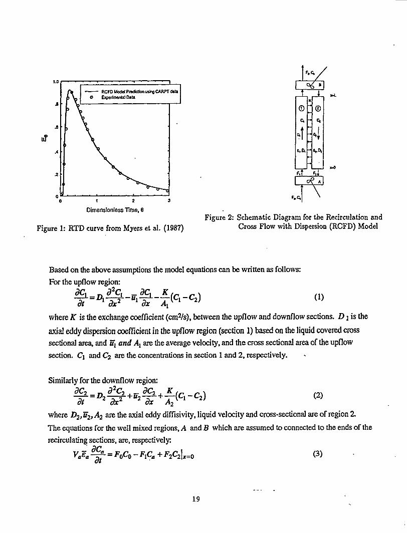
Figure 1: RTD curve from Myers et al. (1987)Figure 2: Schematic Diagram for the Wcirculation and

Cross Flow with Dispersion (RCFD) Model

Based on the above assumptions the model equations can be written as follows

For the upflow regiom

J2C*- ~-~(c, -c,) (1)&L=~~--ul ax Al

at

whereK is the exchangecoefficient (cmZ/s), between the upflow and downflow sections. D 1is the

m“aleddydispersionCoefficientin the upflowregion (section 1) based on the liquidcoveredcrosssectional ~ and i71and Al are the average velocity, and the cross sectional area of the upflow

section. Cl and C2 am the concentrations in section 1 and 2, respectively. ‘

Similarlyfor the downflowRgiom

(2)

where D2,E2,A2are the axial eddy difflsivity, liquid velocity and cross-sectional are of region 2

The equations for the well mixed regions, A and B which are assumed to connected to the ends of the

recirculatingsections, are, respectively

v=;= ;~= Foco - F~c= + F2c&=() (3) - .

----

19

,.. ,...-... ,. . ... . ‘. ,.. .’,,-’-.

,“. . .. . - ,’, ,-., ——. . . . . .

(4)

whereF ois the inlet liquid volumetric flow rate to the co[umnand F’land F2, are the liquid

volumetricflowrates in the upflow section 1and downflowsection 2. V=and V~ are thevolumesand 3=,&kthe average liquid holdup in the two regions. The initial’conditions for a step input of

tmcerat the bottomof the column artxco=~(f) ad Cl=Ca”=Ca=Cb=o @t=o (3

Danckwerts boundaryconditions are used at the inlet of each section with no flux conditions at the

outlet Based on experimental observations, the heights of the two well mixed regions A andB are

assumed to be equal to the diameter of the column.

The avemge upflow and downflow liquid interstitial velocities and holdups, which are required by this

model, are provided as empiriczd input for each condition of interest. This experimental information is

obtained by CA~-Cf’ measurements. The mean liquid velocities are calculated by cross sectional

avenging of the recirculating liquid velocity profile obtained from CA~ measurements. The mean

liquid holdup profiles are similarly obtained from CT measurements. In addition to obtaining the time

averaged flow pammeters, the velocity data from CARIT is used to evaluate the local radial, Dn, and

axial, D= eddy diffusivities. An average value for D= is used for the upflow and for the downflow

region (variation around these vaIues is modest). The cross-flow exchange coefficient, K, is taken to

be equal to the radial eddy diffusivities at the inversion pkme.

In the CARFT technique a single neutrally buoyant radioactive particle, emitting y radiation, is used to

track the motion of the liquid phase. The radiation emitted by the particle is detected by an army of

(h&d)scintillation detectors from which the position of the’particle is calculated as a function of time.

Time differencing of the subsequent positions results in instantaneous bqyangian velocities, which are

ensemble averaged to yield the time averaged velocities of the liquid phase at various locations in the

entire domain of flow (Devanathan, 1991). The scanner for Computed Tomogmphy, CT, (Kumar,

1995) is a transmission type scanner and is capable of obtaining the cross-sectional time averaged

distribution of holdup in a two phase flow system. Since the cross-sectional void fmction

distributions obtained in bubble columns are most often axisymmetric, the distribution can be

circumferentially averaged to ob~”n mdial void fmction profiles.

Exven“mental Results

The tracer response data shown in Figure 1 is from Myers et al. (1987). The tracer experiment was

. . . .20

conducted in a 19 cm diameter cohunn, with a gas supe~lcial velocity of Ug = 10 ~S ~d a liquid

superficial velocity of U1= cm/s in an air-water system. The height of the column is 2.44 m and the

mean residence time of the liquid was reported as 3.2S min. CAR17f-Cf experiments were conducted

under identical conditions to obtain hydrodynamic data for this tracer experimen~ The time averaged

liquid velocity and holdup profiles obtained are shown in Figures 3 and 4, respectively, and are typical

of previously reported XEStdts(Devanathan et al., 1990; Kurnar et ~., 1995). Gas holdup (one minus

liquid holdup) is the highest in the center of the column and the Iowest at the wall (Figure 4), which

causes the hi@est upward liquid velocity in the center of the column and downward liquid flow by the

walls (Figure3),just as incorporated in our model. The mean liquid up!lowand downflowve!oeitks

and correspondingholdupsare computedusing equation (6) and the followingvakes are obtained:El= 12.5cm/s,Fz =7.7cmls, El =0.79 and Z =0.8& An estimate of the axial eddy diffusivities

in the upflow and downflow region is obtained by spatial averaging of the CARPT measured eddydiffusivities in the upflow and dowrdlow section, respectively. These yield D1 = D=, =285 cm2/s

and D2 = ~zz =440 cm2 /s. The average value of the radial diffusivity at the point of velocity

inversionis usedas theestimate of the exchangecoefficient K = ~m, =43 crn2/s.r

J

— Curve Fflo Experimental Data

*

1.0

N1-20 I .7-

1

-.0246 8 10 u .2 .4 .6 .8 1.0

.

RadialPosition,cm NondimensionalRadius

Figure 3: Azimuthally, Axially and Time averaged Figure 4: Azimuthally, Axially and Time AveragedLiquid Axial Velocity Profile Liquid Holdup Profiles

Res k and DISCUSSIQIA.

u .

Comparison of the model predicted impulse tracer response using CARPT-(X results for the

dispersion Coefilcients, holdup and liquid velocities and the measured tracer respse is also shown in

Figure 1. The agreement is good which is remarkable since no free parameters are used to match the

modeI calculated to the observed ‘curve. This provides us with confidence that the RCFD model

describes the mixing phenomena in the column well.

.-, .21

,., . .,,— -. . ... . ... .

500

450

400

350

150

100

50

, ,, I , 1 , ,

,,....●

✎

●

:5

. . ...+---

‘f /

o -! t 1 t I 1 I

o 50 100 150

Figure5: Experimental‘llacer

9

8

7

6

5

4

3

2

1

0

200 250 300 350 400time, s

Responsesin the LaPorte Reactor

I 1 , I , I

.5

h6

.

1, ‘\

t ● ~, ”-’f. \71. \

1; “**.’”+.I

.●

✼

✼

● ✼

“.. \

—1. . . . . . .2

---- 3

----i -“”*.O.S--- ----

, ,

200 300 400 500

I.z.<-

f 4 ‘.%.i .-. .

r —---- ------ .- ._. _ ._ ._. _ .

/A .

-T. ”------ ----~- -y..v. .Y. = .-. ..<. .<.

600 700

Figure 6: ModelCalculatedR&ponsesat DetectorLevels(similarto experiment),for qualitativewith Fig 5 (timescale-isarbitrary)

-.. ... 22

.

Recent tramrstudies conducted during liquid phase methanol (LPMEOH) synthesis runs in the AFDU

oxygenates High Pressure Reactor at the I-Work, Texas, confirm the inadequacy of the ADM and the

promise of RCFDM. The unit is a 46 cm in diameter with liquid dispersion height of about 1300 cm.

Liquid is in the batch mode and tracer is injected at various axial and radiaI locations &lgure 5). Tmcer

responses, subject to injection at N1 close to the wall, were measured at various levels (13gure5) and

cannot be interpreted based on the axial dispersion mcxIel which simply cannot predict the obsemd

overshoots(or dependenceon injectionlocation,not shown). However, for the three detectors(1,23)

furthest fmm the point of injection a monotonicresponseis observed and an axial dispersion

coefficien~which is dependenton locationof the detectors,can be ob~”nedby ~tting the ADMto the

observedresponse. In contrast the RCFDM(Figure6) exhibits serniquantitatively the obseived

responsesat all detector locations. The parametersused to calculate Figure6 were obtainedfor a

columnof smaller diameter and at lower gas velocities. Nevertheless, the essenceof the mixing

patternhas been captured. How changesin diameterand pressureaffect the liquid circulationpattern

and eddy diffusivities is @of the future work,in order to obtain a more quantitativecomparisonof

modelpredictionswith experimentaldata

Devanathan, N., Moslemian, D. and Dudukovid, M.P., 1990, Flow Mapping in Bubble Columns

Using CARPI’, Chern. Engng. Sci.& 2285-2291.

Devanathan,N., Dudukovid,M.P.,Lapin,A. andLubbert,A., 1995,ChaoticFIowin Bubble

ColumnReactors. (3i.em. Engng. Sci. 50,2661-2667.

Devanathan,N., 1991, “Investigationof LiquidHydrodpmics in Bubble Columnsvia

ComputerAutomatedRadioactiveParticIeTracking(CA~, D.SC.Thesis,Washington

University, St. Louis. .

Dudukovid,M.., Deva.nathan,N. and Holub,R., 1991,Multiphase Reactors: Models and

ExperimentalVerification. Revue & I’lnslitutFrancaisdu Petrole 46,439-465.

Dudukovid, M.P. and Devanathan, N., 1993, Bubble Column Reactors: Some Recent Developments,

in Chemical Reactor Technobgy for Erivironnaentilly Safe Reactors (Edited by I-H. D&&a,

et. al), NATO ASI Series R Appl. Sci. 225379-408.

Fan, Liang-Shih, Gas-Liquid-Solid Fluidiza~ion Engineering. Butterworths, 1989.

Grevskott, S., Sanneas, B.H., Dudukovid, M.P., Hjarbo, K.W. and Svendsen, H.F., 1996, Liquid

Circulation, Bubble Size Distributions, and Solids Movement in Two- and three-phase

Bubble Columns, Che. Enng. Sci. 51, 1703-1714.

Kashiw~ B.A. and Gore, R.A., 1991, A Four Equation Model for Multiphase Turbulent Flow.

. ..-

23,

.

... .. . ,,, . . . . . . ...:,, .. ,’. . . . . . . .,.— ,.. ,-- . . ., .,’-

—.2—. ,_____ ..__ __

...

Resented ai the First JoinzASlM?3’JSMEIWdsE@neering Conference.

Krishna, R, Ellenberger, J. and S[e, S.T., 1996, Reactor Development for Conversion of

Natmd Gas to Liquid Fuels: A Scale-up Strategy Relying on Hydrodynamic Analogies,

Chem. Engg. Sci. 51, 2041-2052.Kumar, S.B., Moslemian, D. and Dudukovid, M.P., 1995, A y Ray Scanner for Imaging Voidage

Distributions in Two Phase Fiow Systems. Flow Measurementand Instrumentation 6,

61-63, 1995.

Myers, K.J., Dudukovid, M.P. and Ramachandran, P.A., 1986, Modeling of Chum-Turbulent

Bubble Columns -1: Liquid Phase Mixing. Chem. 13zgng.Sci. 42,2301-2311.

Sokolichin, A., Eigenlxrger, G., 1995, Gas-Liquid Flow in Bubble Columns and Loop

Raictorx Part I. Detailed Modeling and Numerical Simulation. Chem. Dzgng. Sci.

49, 5735-5746.

Svendsen, I-I.F.,Jakobsen, H.A. and Torvik, R., 1992, Local Flow Structures in Internal

Loop and Bubble Column Reactom. Clzem. Engng. Sci. 47,3299-3304.

Wilkinson, P.M., Haringa, H. Stokrnan, F.P.A. and van Dierendonck, L.L., 1993, Liiquid

Mixing in Bubble Columns Under Pressure. Chem. Engng. Sci. 48, 1785-1791.

Yang, Y.B., Devanathanb, N. and Dudukovid, M.P., 1993, Liquid Backmixing in Bubble

Columns via Computer-Automated Radi~tive Particle Tmcking (CARPI’). Exp.

Fluids 16, 1-9.

. . . .

24

Task 3.3- Sparger ModelingInitial work on developing an understandingof the importanceof the spargerin a SBCRconsists of the initiation of a literature search and preliminary meetings and discussionswith Sandia, Ohio State and Washington University personnel to understand theframework for an experimental study. The complete analysis of the literature searchawaits conclusion of detailed reading of the documents and the final step of developing asearch strategy. This section is a preliminary report on the progress of the search and asummary of the presentation made at Sandia that was based on that work.

Literature Search-PreliminaryResults

Twenty-sixdocumentswerefoundin a standardsearchl. Agoodreviewof the olderliteratureis foundin Decker(l), whileHebrardet al. (2)providea morerecentsummary.Despite these summaries, no clear pattern emerges on the effect of a sparger on even asimple parameter like overall holdup for bubble columns. In addition, only one referencewas found for a sparger change for systems with solids (3).

The effect of gas distributor and material properties on &g[gas holdup] is complex (l).

Large differences in holdup with sparger type are measured at low (e10’cm/see) gasvelocities. Much of the difference is explained by changes in the onset of transition or thepresence of imperfect bubble flow (2). These issues may not be applicable to the highflow rates of thi chum turbulent flow regime.

Most of the data pertain to water/air, which is a high surface tension system and maybehave very differently from low surface tension organic systems. Most measurements areat or near atmospheric pressure. The effects of pressure and increased solids loading areunclear. In most cases, the effects of sparger differences diminish as flow rate increases.Commonly studied spargers, for example, sintered metal plates, porous plates and rubberdiaphragms, are useful for developing information, but are not practical for industrialsituations that use catalyst.

In summary, the literature can provide some insight into what parameters should beconsidered in sparger design. However, insufficient information is available for sparger

lData bases searched and search strategy are given below.Engineering Index, Chemical Engineering and Biotech. Abstracts, NTIS

Databases

Sparg?(within 10 words of) slurry (within 10 words of) bubble column? or

and

reactor?; alsogas inlet or intake and bubble column? or reactor?

in a second searchSearch terms: Sparging - keyword; plus bubble columns - keyword

. . . .

.

. .—... _ —..—.— _—

design for industrial systems at high gas flow rates and elevated pressures. The majorfindings from the search are that good design methods do not exis~ and additionalexperimental work is needed to begin to understand the importance of various spargerparameters on column performance.

Design IssuesA sparger has only one function--introductionof gas to the reactor. However,gasdistributioncan influencethe performanceof the bubblecolumnin severalways:●

●

●

●

bubble size distribution, which in turn can affect mass transferradial bubble distribution, which is a measure of uniformity and, therefore, reactorutilization

uniformity of solids distributionerosion of the vessel or internal walls

Thus, one mustconsider the method of bubble generation, as well as the type ofdistributor and its placement in the reactor in any study of the function of the distributor.

The objective of the experimental study will be to ascertain the importance of spargerdesign when the reactor is operating in the chum turbulent regime of slurry bubble columnflow. It is clear that a single pipe sparger might not give adequate gas distribution. Whatis not clear is the importance of hole size in obtaining a uniform degree of mixedness in aSBCR. Similarly, uniform flow may not be achieved if the sparger is placed at the edge ofthe radius of the column, but the degree of maldistribution allowed while a uniformdistribution is maintained is not at all clear. An initial sparger study should answerquestions such as. What is the importance of sparger hole size?. What is the sensitivity of the degree of mixedness of the system to sparger placement?

In short,

● What degree of care must be taken to have a well-mixed system?This study is intended to gain an understanding of what constitutes an adequate spargersystem.

Bubble FormationIn general, three conditions of bubble formation have been identified: a constant flowcondkion, a constant pressure condition, and a condition intermediate between the two.Somewhat surprisingly, the size of a bubble can depend upon the volume of the spargerchamber for the latter two cases (4). Bubble formation can be divided further byconsidering the gas flow rate. At high gas flow rates (Nw> 16, where Nw=BoFrO”5andBo=pD2g/o and Fr=U2/Dg), the dependence of bubble formation on the sparger chamberis minimized. This is especially true when the pressure drop across the hole is high relativeto the pressure fluctuations in the bubble during formation. For the conditions iypicallyfound in the LaPorte reactor, Nwis greater than 16. This eases the design problemsomewhat. However, laboratory studies should always be carried out in this region aswell. This means careful planning of sparger hole size and gas flow rates so that even forthe largest size holes being tested, NW,is greater than 16 and the pressure drop across the

. . .

orifice is high relative to the fluctuations during bubble formation so that bubble sizefactors can be isolated from the other changes made.

Sparger TypeSpargers made from sintered plates and pipes, porous plates and flexible diaphragms havebeen used for most academic studies. However, the presence of the fine catalyst particlesprecludes using these types of spurges in a commercial reactor. Other sparger types, forexample, rings, doughnuts and crosses, have been used sparingly in academic studies.However, since these types of spargers should provide a much better simulation of anactual industrial-scale sparger, they should be the primary devices. A device such as aporous plate, which gives uniform distribution, should, of course, be used when a

comparison with complete uniformity is desired. Hole orientation, up or down, shouldalso be considered as part of this initial study. Maldistribution can be simulated byblocking one-half or one-quarter of the area of such a device.

References1. Deckwer, W. D. Bubble Column Reactors, 1992, John Wiley and Sons, p. 170H2. Hebrard, G., Bastoul, D., Roustan, M. TransI Chenz E, Vol. 74 Part A, April 1966, p.406ff.3. Smith, G. B., Garnblin, B. R. and Newton, D. Trans I Chenz E, Vol 73, Part A,Augus~ 1995, p. 632 ff.4. Tsuge, H. Hvdrodmamics of Bubble Formation From Submermxl Orifices inEncYclomxliaof Fluid Mechanics, N. Cheremisinoff, Gulf Publishing Co. 1986, p. 1931.