Embed Size (px)
Citation preview

ENGG3190“Introduction to Optimization”
Winter 2014
S. Areibi
School of Engineering
University of Guelph

Outline
2
• OptimizationOptimization• Linear ProgrammingLinear Programming
– DefinitionDefinition– FormulationFormulation– Simplex MethodSimplex Method
• Integer Linear ProgrammingInteger Linear Programming– DefinitionDefinition– FormulationFormulation– ComplexityComplexity– Branch and & BoundBranch and & Bound

IntroductionIntroduction• Optimization is the act of obtaining the best result best result under given
circumstances.
• Optimization can be defined as the process of finding the conditions that:– Give the maximummaximum of a function, or– Give the minimumminimum of a function.
• The optimum seeking methods are also known as mathematical programming techniques and are generally studied as a part of operations research.
3

Classification of Optimization ProblemsContinuous Optimization Unconstrained Optimization Bound Constrained Optimization Derivative-Free Optimization Global Optimization Linear Programming Network Flow Problems Nondifferentiable Optimization Nonlinear Programming Optimization of Dynamic Systems Quadratic Constrained Quadratic Programming Quadratic Programming Second Order Cone Programming Semidefinite Programming Semiinfinite Programming Discrete and Integer Optimization Combinatorial Optimization
Traveling Salesman Problem Integer Programming
Mixed Integer Linear Programming Mixed Integer Nonlinear Programming
Optimization Under Uncertainty Robust Optimization Stochastic Programming Simulation/Noisy Optimization Stochastic Algorithms Complementarity Constraints and Variational Inequalities Complementarity Constraints Game Theory Linear Complementarity Problems Mathematical Programs with Complementarity Constraints Nonlinear Complementarity Problems Systems of Equations Data Fitting/Robust Estimation Nonlinear Equations Nonlinear Least Squares Systems of Inequalities Multiobjective Optimization
4

Convex functionsConvex functionsDefinition #1: A function f(x) is convex in an interval if its second derivative is positive on that interval.Example: f(x)=x2 is convex since f’(x)=2x, f’’(x)=2>0
5

Convex functionsConvex functionsThe second derivative test is sufficient but not necessary.
Definition #2: A function f(x) is convex if a line drawn between any two points on the function remains on or above the function in the interval between the two points.
6

Convex functionsConvex functionsDefinition #2: A function f(x) is convex if a line drawn between any two points on the function remains on or above the function in the interval between the two points.
Is a linear function convex?Is a linear function convex?
Answer is “yesyes” since a line drawn between any two points on the function remains on the function. 7

Convex SetsConvex SetsDefinition #3: A set C is convex set C is convex if a line segment between any two points in C lies in C.
Ex: Which of the below are convex sets?
8
convexNon-convex

Convexity & global vs. local optimaConvexity & global vs. local optimaWhen minimizing a function, if we want to be sure that we can get a global solution global solution via differentiation, we need to impose some requirements on our objective function. We will also need to impose some requirements on the feasible set S (set of possible values the solution x* may take).
Min f(x)subject toh(x)=cg(x)> b Sx
xf
subject to
)(min
Definition: If f(x) is a convex function, and if S is a convex set, then the above problem is a convex programming problem.
Definition: If f(x) is not a convex function, or if S is not a convex set, then the above problem is a non-convex programming problem. 9
Feasible set

Convex vs. nonconvex programming problemsConvex vs. nonconvex programming problems
The desirable quality of a convex programming problem is that any any locally locally optimal solutionoptimal solution is also a a globally globally optimal solutionoptimal solution. If we have a method of finding a locally optimal solution, that method also finds for us the globally optimum solution.
10
The undesirable quality of a non-convex programming problem is that any method which finds a locally optimal solution does not necessarily find the globally optimum solution.globally optimum solution.
MATHEMATICAL PROGRAMMING
Convex
Non-convex
We address convex programming problems in addressing linear programming.
We will also, later, address a special form of non-convex programming non-convex programming problems called integer integer programs.programs.

Calculus Based MethodsCalculus Based Methods
0dxdF
Assume F is known analytically and twice differentiable. The critical pointsof F, ie the points of potential maximum or minimum, are given by equation
(1)
Once the roots x1, x2, …., xN of (1) are found, the sign of the second derivativetells if each of those points is a maximum or a minimum:
02
2
dxFd
If for x=xj, then x=xj is a minumum
If 02
2
dxFd for x=xj, then x=xj is a maximum
If the second derivative is 0 in a critical point xj then xj may or may not be a minimum or a maximum of F.

Intel chip manufacturing
• Consider the following hypothetical problem– x = sales price of Intel’s newest chip (in $1000’s of dollars)
– F(x) = profit per chip (in $1000’s of dollars).
– Assume that Intel’s marketing research team has found that the profit per chip (as a function of x) is
F(x) = x2 - x3
– Assume that we must have x non-negative and no greater than 1
• Set this up as an optimization problem:– objective function is profit F(x) that needs to be maximized
– solution to the optimization problem will be the optimum chip sales price

Differentiating: Solving Intel Manuf. Example
• Since we know f(x) analytically, we can find d/dx f(x) = 2x - 3x2
• Setting this to 0, we get 2x = 3x2 and hence x0 = 2/3 is a critical point
• d2/dx2 f(x) =2-6x, and, when x=x0=2/3,
we have d2/dx2 f(x0) = -2 < 0, so x0 is a maximum
• So, the optimal price per chip is $667 maximizes the profit
f(x)
x0.0 1.00.0
0.15

General Statement of Optimization ProblemGeneral Statement of Optimization Problem
)x(Fmin Dx )x(Fmax Dx
where x - input variable, scalar or vector valuedD - domain for x over which optimization is performedF - objective function, can be computed or known analytically
or
If there are no constraints then the problem is an unconstrained Optimization

General Statement of Optimization ProblemGeneral Statement of Optimization Problem
Note: we can always replace maximization problem with an equivalent minimization problem.
)x(Fmin)x(Fmax DxDx -

Constrained OptimizationConstrained Optimization
• Mathematical optimization problem:
• f0 : Rn R: objective function• x=(x1,…..,xn): design variables (unknowns of the problem,
they must be linearly independent)
• gi : Rn R: (i=1,…,m): inequality constraints
• The problem is a constrained optimization problem
mibxg
xf
ii ,....,1,)( subject to
)( minimize 0

17
ConstraintsConstraints
• Behaviour constraints: Constraints that represent limitations on the behaviour or performance behaviour or performance of the system are termed behaviour or functional constraints.
• Side constraints: Constraints that represent physical limitations on design variables such as manufacturing limitations.

Problem Formulation• What is the objective?
– Maximize profit,– Minimize inventory, ...– Minimize time to schedule, …
• What are the decision variables?– Capacity, routing, production and stock levels
• What are the constraints?– Capacity is limited by capital– Production is limited by capacity

19
Linear ProgrammingLinear Programming

20
Linear Programming: ApplicationsLinear Programming: Applications
• The Importance of Linear Programming– Many real world problems lend themselves to linear programming modeling. – Many real world problems can be approximated by
linear models.– There are well-known successful applications in:
• ManufacturingManufacturing• MarketingMarketing• Finance (investment)Finance (investment)• AdvertisingAdvertising• AgricultureAgriculture• LogisticsLogistics• ManagementManagement
• EngineeringEngineering• VLSI DesignVLSI Design• Logic SynthesisLogic Synthesis• High Level SynthesisHigh Level Synthesis• Physical SynthesisPhysical Synthesis

Introduction to Linear ProgrammingIntroduction to Linear Programming
• A Linear Programming model seeks to maximize or minimize a linear function, subject to a set of linear constraints.
• The linear model consists of the followingcomponents:– A set of decision variables.– An objective function.– A set of constraints.
21

22
Max 8X1 + 5X2 (Weekly profit)
subject to
2X1 + 1X2 1000 (Plastic)
3X1 + 4X2 2400 (Production Time)
X1 + X2 700 (Total production)
X1 - X2 350 (Mix)
Xj > = 0, j = 1,2 (Nonnegativity)
Linear Programming ModelLinear Programming Model• Decisions variables::
– X1 = Weekly production level of toy#1 (dolls) (in dozens)
– X2 = Weekly production level of toy#2 (…) (in dozens).
• Objective Function: (maximize the weekly profit)
– $8 profit for toy #1, 5$ profit for toy #2
• Constraints: (1000 pounds of plastic, 40 hours of production time)
– Toy#1 requires 2 pounds of plastic, 3 minutes of labor per dozen
– Toy#2 requires 1 pound of plastic, 4 minutes of labor per dozen
This can be easilyThis can be easilysolved using thesolved using theSimplex Method.Simplex Method.
CPLEX Package CPLEX Package in SOEin SOE

23
The non-negativity constraints
X2
X1
Graphical Analysis – the Feasible RegionGraphical Analysis – the Feasible Region

24
1000
500
Feasible
X2
Infeasible
Production Time3X1+4X2 2400
Total production constraint: X1+X2 700 (redundant)
500
700
The Plastic constraint2X1+X2 1000
X1
700
Graphical Analysis – the Feasible RegionGraphical Analysis – the Feasible Region

25
1000
500
Feasible
X2
Infeasible
Production Time3X1+4X22400
Total production constraint: X1+X2 700 (redundant)
500
700
Production mix constraint:X1-X2 350
The Plastic constraint2X1+X2 1000
X1
700
Graphical Analysis – the Feasible RegionGraphical Analysis – the Feasible Region
• There are three types of feasible pointsInterior points. Boundary points. Extreme points.

26
The search for an optimal solutionThe search for an optimal solution
Start at some arbitrary profit, say profit = $2,000...Then increase the profit, if possible...
...and continue until it becomes infeasible (extreme point)
Profit =$4360
500
700
1000
500
X2
X1
Objective Function Max 8X8X11 + 5X + 5X22

27
Summary of the optimal solution Summary of the optimal solution
Toy #1 = 320 dozen Toy #2 = 360 dozen Profit = $4360
– This solution utilizes all the plastic and all the production hours.
– Total production is only 680 (not 700).
– Toy#2 production exceeds Toy#1 production by only 40 dozens.

28
– If a linear programming problem has an optimal solution, an extreme point is optimal.
Extreme points and optimal solutionsExtreme points and optimal solutions

29
• For multiple optimal solutions to exist, the objective function must be parallel to one of the constraints
Multiple optimal solutionsMultiple optimal solutions
•Any weighted average of optimal solutions is also an optimal solution.

30
Example II: Standard ModelExample II: Standard Model
2,
6
9
s)(lubricant 5.03.02.0
fuel)(jet 5.12.04.0
(gasoline) 0.24.03.0s.t.
21
2
1
21
21
21
xx
x
x
xx
xx
xx
21 1520min xx

31
Graphing Constraints
1x
2x
Variable-TypeConstraints(must be positive)

32
Adding Main Constraints
1x
00.54.0
2,0
67.63.0
2,0
24.03.0
21
12
21
xx
xx
xx
2x

33
Next Constraint
1x 67.13.0
5.0,0
50.22.0
5.0,0
5.03.02.0
50.72.0
5.1,0
75.34.0
5.1,0
5.12.04.0
21
12
21
21
12
21
xx
xx
xx
xx
xx
xx2x

34
Final Constraints
1x
62 x
91 x
FeasibleRegion
2x

35
Finding Optimal Solution
1x
2x
21 1520 xx

36
Optimal Solution
1x
2x
5.925.315220
1520 21
xx
21 x
5.31 x

Solver for Linear ProgrammingSolver for Linear Programming
• Problems casted as linear programming models can be efficiently solved using:– Simplex Method
– Interior Point Methods O(n3)
• CPLEX is an excellent solver
• If variables are restricted to integer values then the problem is much difficult to solve and is modeled as an Integer Linear Programming problem (ILP)
37

38
Integer Linear ProgrammingInteger Linear Programming

Discrete Variables• Linear programming allows us to
solve large scale optimization problems. It gives answers in terms of continuous variables
• However, there are many situations where we need solutions to optimization problems which are not allowed to fall in a continuous range

Design Problem
• For example, if we are designing a network, we need to decide whether to place a link between two particular nodes
• In this case a decision is either “yes” or “no”.
• We could represent this as a variable which had only two possible values, 0 or 1

Page 41
Traveling Salesman ProblemFind shortest tours that visit all of n cities.

Types of ILP Models
ILP:
A linear program in which some or all variables are restricted to integer values.
Types: 1. All-integer LP (ILP)
2. Mixed-Integer LP (MIP)
3. 0-1 integer LP (BIP)

Example of ILPExample of ILP
Max Z = 5x1 + 8x2
s.t. x1 + x2 6
5x1 + 9x2 45
x1 , x2 ≥ 0 integer
x1 + x2 = 6
5x1 + 9x2 = 45
0
1
2
3
4
5
6
1 2 3 4 5 6 7 8
(2.25, 3.75)
Z=41.25
Z=20

Page 44
ILP vs. LP
lu
z
• Why is ILP more difficult to solve than LP?• Because the solution is not restricted to the
vertices of the feasible region but all integer values inside the feasible region.
• This is a Combinatorial Optimization Problem.

Combinatorial Explosion
A 10 city TSP 10 city TSP has 181,000 possible solutions
A 20 city TSP 20 city TSP has 10,000,000,000,000,000 possible solutions
A 50 City TSP 50 City TSP has 100,000,000,000,000,000,000,000,000,000,000,000,000,000,000,000,000,000,000,000,000 possible solutions!!!!!!!
There are 1,000,000,000,000,000,000,000 litres of water on the planet
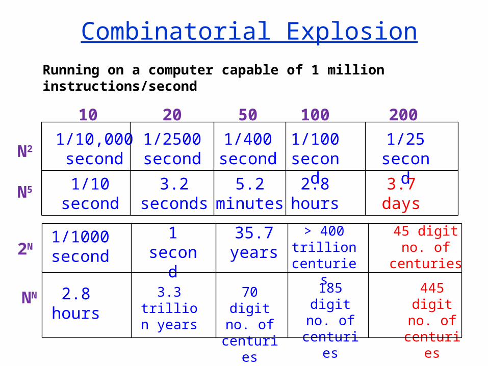
Combinatorial Explosion
10 20 50 100 200
N2
N5
1/10,000 second
1/2500 second
1/400 second
1/100 second
1/25 second
1/10 second
3.2 seconds
5.2 minutes
2.8 hours
3.7 days
2N
NN
1/1000 second
1 second
35.7 years
> 400 trillion
centuries
45 digit no. of centuries
2.8 hours
3.3 trillion years
70 digit no. of
centuries
185 digit no. of
centuries
445 digit no. of
centuries
Running on a computer capable of 1 million instructions/second

An All-Integer IP or Pure ILP
Maximise 2 x1 + 3 x2
Subject to
3 x1 + 2 x2 ≤ 12
¼ x1 + 1 x2 ≤ 4
1 x1 + 2 x2 ≤ 6
x1, x2 ≥ 0 and integer

Linear Programming v Integer Linear Programming v Integer ProgrammingProgramming
An LP
Minimise X2
Subject to: 2X1+X2 >=13
5X1+2X2<=30
-X1+X2 >=5
X1 , X2 >= 0
The Solution
• X1 = 22/3 , X2 = 72
/3
The Solution
• X1 = 2 , X2 = 9
An IP
Minimise X2
Subject to: 2X1 + X2 >=13
5X1 + 2X2<=30
-X1 + X2 >=5
X1 , X2 >= 0 and integer

Example of Integer Program(Production Planning-Furniture
Manufacturer)• Technological data:
Production of 1 table requires 5 ft pine, 2 ft oak, 3 hrs labor
1 chair requires 1 ft pine, 3 ft oak, 2 hrs labor
1 desk requires 9 ft pine, 4 ft oak, 5 hrs labor• Capacities for 1 week: 1500 ft pine, 1000 ft oak,
20 employees (each works 40 hrs).• Market data:
• Goal: Find a production schedule for 1 week
that will maximize the profit.
profit demand
table $12/unit 40
chair $5/unit 130
desk $15/unit 30

Production Planning-Furniture Manufacturer: modeling the problem as
integer program
The goal can be achieved
by making appropriate decisions.
First define decision variables:
Let xt be the number of tables to be produced;
xc be the number of chairs to be produced;
xd be the number of desks to be produced.
(Always define decision variables properly!)

Production Planning-Furniture Manufacturer: modeling the problem as
integer program Objective is to maximize profit:
max 12xt + 5xc + 15xd
Functional Constraints
capacity constraints:
pine: 5xt + 1xc + 9xd 1500
oak: 2xt + 3xc + 4xd 1000
labor: 3xt + 2xc + 5xd 800
market demand constraints:
tables: xt ≥ 40
chairs: xc ≥ 130
desks: xd ≥ 30
Set Constraints
xt , xc , xd Z+

Example of IP: Facility Location
• A company is thinking about building new facilities in LA and SF.
• Relevant data:
Total capital available for investment: $10M
• Which facilities should be built Which facilities should be built to maximize profit?
capital needed expected profit1. factory in LA $6M $9M2. factory in SF $3M $5M
3. warehouse in LA $5M $6M4. warehouse in SF $2M $4M

Example of IP: Facility Location
• Define decision variables (i = 1, 2, 3, 4):
• Then the total expected benefit: 9x1+5x2+6x3+4x4
the total capital needed: 6x1+3x2+5x3+2x4
Summarizing, the IP model is:
max 9x1+5x2+6x3+4x4
s.t. 6x1+3x2+5x3+2x4 10
x1, x2, x3, x4 binary ( i.e., xi {0,1} )
not if 0
built is facility if 1x i
i

Page 54
Subproblems/Applications
• Facility locationLocating warehouses or franchises (e.g., a Burger King)
• Set covering and partitioningScheduling airline crews, Logic Synthesis, HLS
• Multicommodity distributionDistributing auto parts
• Traveling salesman and extensionsRouting deliveries
• Capital budgeting• Other applications
VLSI layout, clustering

Page 55
Traveling Salesman Problem
Find shortest tours that visit all of n cities.
courtesy: Applegate,
Bixby, Chvátal, and Cook

Page 56
Traveling Salesman Problem
cij = cji = distance from city i to city j (assuming symmetric version)xij if tour goes from i to j or j to i, and 0 otherwise
Anything missing?
n
i
n
jijij xc
1 1
nixn
jij
120
(path enters and leaves)
minimize:
subject to:
binary , ijji xx

Page 57
Traveling Salesman Problem
cij = distance from city i to city j
xij = 1 if tour visits i then j, and 0 otherwise (binary)
ti = arbitrary real numbers we need to solve for
n
i
n
jijij xc
1 1
njinnxtt
njx
nix
ijji
n
iij
n
jij
,21
11
11
0
0
(out degrees = 1)
(in degrees = 1)
(??)(??)
minimize:
subject to:

Page 58
Traveling Salesman Problem
The last set of constraints: prevents “subtours”:
njinnxtt ijji ,21

Page 59
Set Covering Problem
Find cheapest sets that cover all elements
Courtesy: Darmstadt University of Technology

Page 60
Set Covering and Partitioning
Given m sets and n items:
otherwise 0,
included is jset if ,1jset ofcost
otherwise ,0
i item includes jset if ,1
j
i
ij
x
c
AColumns = setsRows = items
Set covering:minimize: cTx
subject to: Ax ≥ 1, x binary
Set partitioning:minimize: cTx
subject to: Ax = 1, x binary

296.3 Page 61
Set Covering and Partitioning
Best cover: s2, s4, s5 = .5
Best partition: s4, s6 = .7
setmembers
cost
s1 {a,c,d} .5
s2 {b,c} .2
s3 {b,e} .3
s4 {a,d} .1
s5 {c,e} .2
s6 {b,c,e} .6
s7 {c,d} .2
0110100
1001001
1110011
0100110
0001001
A

Page 62
Set Covering and Partitioning
Applications:• Facility location.
Each set is a facility (e.g., warehouse, fire station, emergency response center).Each item is an area that needs to be covered
• Crew scheduling.Each set is a route for a particular crew member (e.g. NYC->Pit->Atlanta->NYC).Each item is a flight that needs to be covered.
• Logic Synthesis Each set is prime implicant and each item is min
term.

Page 63
Algorithms
1. Relax the IP (let variables be continous) and use a linear program (solutions are fractions)– round to integer solution
• What if not feasible?• How far away from Optimal Solution??
2. Search– Branch and bound (integer ranges)– Implicit (0-1 variables)

Relaxation of the ILP ModelRelaxation of the ILP Model
Maximize 10T + 15A
Subject to: 282T + 400A ≤ 2000
4T + 40A ≤ 140
T ≤ 5
T, A ≥ 0 and integer
Sweeny: Eastborne Reality is considering investing in townhouses (T)townhouses (T) and apartments(A)apartments(A).
• Determine the number of T’s and A’s to be purchased. (Integers)Determine the number of T’s and A’s to be purchased. (Integers)
Funds available: $2 million.Cost: $282k per T and $400k per A
Numbers available: 5 T’s and any number of A’s.
Management time available: 140 h/moTime needed: 4 hrs/mo for T and 40 h/mo for A.
Contribution: $10k for T and $15k for A.
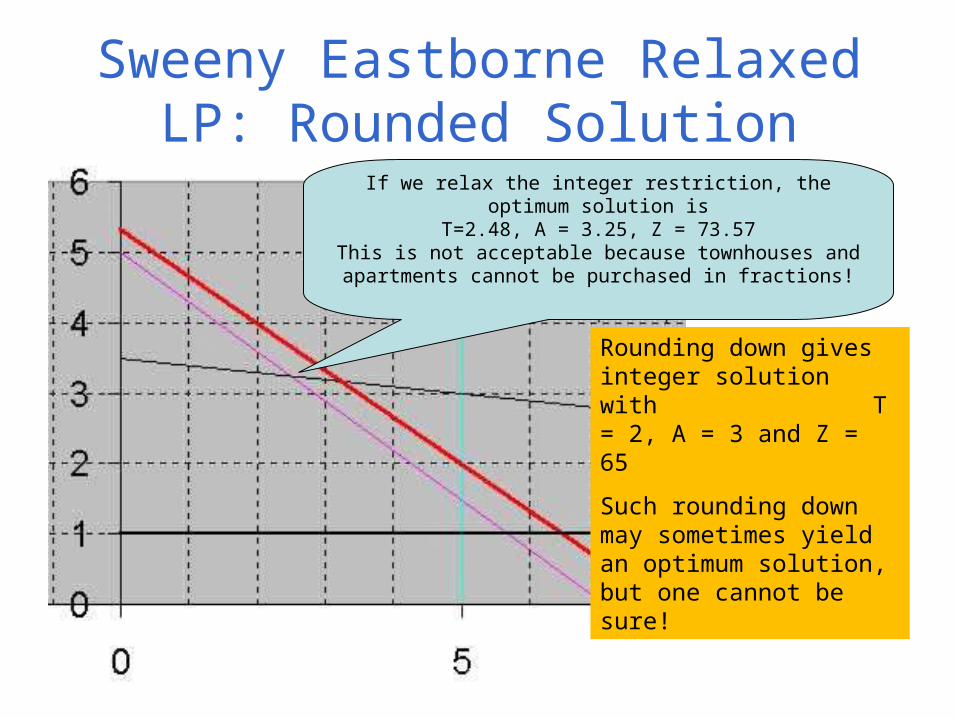
Sweeny Eastborne Relaxed LP: Rounded Solution
If we relax the integer restriction, the optimum solution is
T=2.48, A = 3.25, Z = 73.57This is not acceptable because townhouses and
apartments cannot be purchased in fractions!
Rounding down gives integer solution with T = 2, A = 3 and Z = 65
Such rounding down may sometimes yield an optimum solution, but one cannot be sure!

Sweeny Eastborne ILPOptimal Integer Solution
The optimal solution is T = 4, A = 2, Z = 70 and not the rounded-down solution which
gives Z = 65.

Page 67
Important Properties
• If you relax the IP (make the variable continuous instead of integers or 0-1) then– The LP solution is an upper bound on IP
solution (assuming maximization)– The LP solution is a lower bound on the IP
solution (assuming minimization)
• If LP is infeasible then IP is infeasible
• If LP solution is integral (all variables have integer values), then it is the IP solution.

68
Branch and Bound Algorithm
• Branch and bound algorithms are the most popular methods for solving integer programming problems
• They enumerate the entire solution space but only implicitly; hence they are called implicit enumeration algorithms.
• Running time grows exponentially with the problem size, but small to moderate size problems can be solved in reasonable time.
Page 69
Branch and Bound
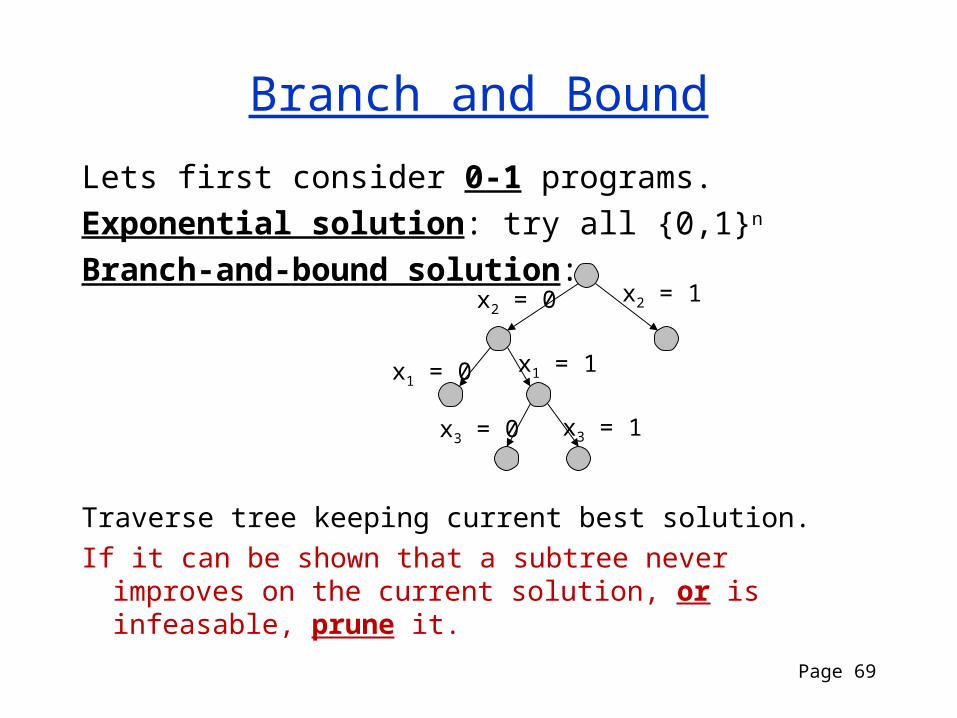
Lets first consider 0-1 programs.Exponential solution: try all {0,1}n
Branch-and-bound solution:x2 = 0 x2 = 1
x1 = 0 x1 = 1
x3 = 0 x3 = 1
Traverse tree keeping current best solution.If it can be shown that a subtree never improves on
the current solution, or is infeasable, prune it.

Example of ILPExample of ILP
Max Z = 5x1 + 8x2
s.t. x1 + x2 6
5x1 + 9x2 45
x1 , x2 ≥ 0 integer
x1 + x2 = 6
5x1 + 9x2 = 45
0
1
2
3
4
5
6
1 2 3 4 5 6 7 8
(2.25, 3.75)
Z=41.25
Z=20

Utilizing the information about the optimal solution of the LP-relaxation
Fact: If LP-relaxation has integral optimal solution x*, then x* is optimal for IP too.
In our case, (x1, x2) = (2.25, 3.75) is the optimal solution of the LP-relaxation. But, unfortunately, it is not integral.
• The optimal value is 41.25 .
Fact: OPT(LP-relaxation) ≥ OPT(IP)
(for maximization problems)
That is, the optimal value of the LP-relaxation
is an upper bound
for the optimal value of the integer program.• In our case, 41.25 is an upper bound for OPT(IP).

Branching step• In an attempt to find out more
about the location of the IP’s optimal solution,partition the feasible region of the LP-relaxation.
• Choose a variable that is fractional in the optimal solution to the LP-relaxation – say, x2 . Observe that every feasible IP point must have either x2 3 or x2 ≥ 4 .
• With this in mind, branch on the variable x2 to create the following two subproblems:
Subproblem 1 Subproblem 2Max Z = 5x1 + 8x2 Max Z = 5x1 + 8x2
s.t. x1 + x2 6 s.t. x1 + x2 6 5x1 + 9x2 45 5x1 + 9x2 45
x2 3 x2 ≥ 4 x1 , x2 ≥ 0 x1 , x2 ≥ 0
• Solve both subproblems (note that the original optimal solution (2.25, 3.75) can’t recur)

Branching step (graphically)
Subproblem 1: Opt. solution (3,3) with value 39
Subproblem 2: Opt. solution (1.8,4) with value 41
0
1
2
3
4
5
1 2 3 4 5 6 7 8
Z=20
Subproblem 1
Subproblem 2
(1.8, 4)
(3, 3)
Z=39
Z=41

Solution tree
For each subproblem, we record• the restriction that creates the subproblem• the optimal LP solution• the LP optimum value
The optimal solution for Subproblem 1 is integral: (3, 3). If further branching on a subproblem will yield no useful
information, then we can fathom (dismiss) the subproblem. In our case, we can fathom Subproblem 1 because its solution is integral.
The best integer solution found so far is stored as incumbent. The value of the incumbent is denoted by Z*.
In our case, the first incumbent is (3, 3), and Z*=39.
Z* is a lower bound for OPT(IP): OPT(IP) ≥ Z* . In our case, OPT(IP) ≥ 39. The upper bound is 41: OPT(IP) 41.
All
(2.25, 3.75)
Z=41.25
S1: x2 3
(3, 3)
Z=39
S2: x2 ≥ 4
(1.8, 4)
Z=41
int.

Next branching step (graphically)
- Fathom Subproblem 1.
- Branch Subproblem 2 on x1 :
Subproblem 3: New restriction is x1 1.
Opt. solution (1, 4.44) with value 40.55
Subproblem 4: New restriction is x1 ≥ 2.
The subproblem is infeasible
0
1
2
3
4
5
1 2 3 4 5 6 7 8
Z=20
Subpr. 3 Subpr. 4
Z=40.55
(1, 4.44)

Solution tree (cont.)
If a subproblem is infeasible, then it is fathomed.In our case, Subproblem 4 is infeasible; fathom it.
The upper bound for OPT(IP) is updated: 39 OPT(IP) 40.55 .
Next branch Subproblem 3 on x2 .
(Note that the branching variable might recur).
All
(2.25, 3.75)
Z=41.25
S1: x2 3
(3, 3)
Z=39
S2: x2 ≥ 4
(1.8, 4)
Z=41
int.S3: x1 1
(1, 4.44)
Z=40.55
S4: x1 ≥ 2
infeasible

Next branching step (graphically)
Branch Subproblem 3 on x2 :
Subproblem 5: New restriction is x2 4.
Feasible region:
the segment joining (0,4) and (1,4)
Opt. solution (1, 4) with value 37
Subproblem 6: New restriction is x2 ≥ 5.
Feasible region is just one point: (0, 5)
Opt. solution (0, 5) with value 40
0
1
2
3
4
5
1 2 3 4 5 6 7 8
Z=20
(1, 4)
(0, 5)

Solution tree (final)
If the optimal value of a subproblem is Z*, then it is fathomed.• In our case, Subproblem 5 is fathomed because 37 39 = Z*.
If a subproblem has integral optimal solution x*, and its value > Z*, then x* replaces the current incumbent.• In our case, Subproblem 5 has integral optimal solution, and its value
40>39=Z*. Thus, (0,5) is the new incumbent, and new Z*=40.
If there are no unfathomed subproblems left, then the current incumbent is an optimal solution for (IP). • In our case, (0, 5) is an optimal solution with optimal value 40.
All
(2.25, 3.75)
Z=41.25
S1: x2 3
(3, 3)
Z=39
S2: x2 ≥ 4
(1.8, 4)
Z=41
int.S3: x1 1
(1, 4.44)
Z=40.55
S4: x1 ≥ 2
infeasible
S5: x2 4
(1, 4)
Z=37
S6: x2 ≥ 5
(0, 5)
Z=40
int.
int.

79
NP-completeness
Do your best then.

Heuristics
Heuristics
Meta-heuristicsLocal Search
Single PointPopulation
Based
Tabu SearchSimulatedAnnealing
GeneticAlgorithms
ParticleSwarm
AntColony

81

ILP AlgorithmsILP Algorithms
The ILP algorithms are based on exploiting the tremendous computational success of LP. The strategy involves three steps:
1. Relax the ILP: Remove integer restrictions; replace any binary variable y with continuous range 0 y 1.
2. Solve the relaxed LP as a regular LP.
3. Starting with the relaxed optimum, add constraints that iteratively modify the solution space to satisfy the integer requirements.

ExampleExample
Max Z = 21x1+11x2
s.t. 7x1+4x2 ≤13
x1 ≥0, x2 ≥0
x1 ,x2 are integers

Example (cont.)Example (cont.)
Step 0: Create Problem 1. Step 1: Remove Problem 1
from the master list. Step 2: Solve Problem 1. Step 3: Branch on X1, since
X1 not integer-valued. Step 4: Create Problem 2 & 3.
Place on master list.

Example (cont.)Example (cont.)
Step 1: Remove Problem 2 from the master list.
Step 2: Solve Problem 2. Step 3: No feasible solution.
Stop.

Example (cont.)Example (cont.)
Step 1: Remove Problem 3 from the master list
Step 2: Solve Problem 3 Step 3: Branch on X2, since
X2 not integer-valued Step 4: Create Problem 4 & 5
place on master list

Example (cont.)Example (cont.)
Step 1: Remove Problem 4 from the master list.
Step 2: Solve Problem 4. Step 3: Solution satisfies integer
constraint. Record the solution and stop!

Example (cont.)Example (cont.)
Following the same steps,terminate computationsuntil master list is empty.

Branch-and-Bound (B&B)Branch-and-Bound (B&B)
• Developed in 1960 by A Land and G Doig
• Relax the integer restrictions in the problem and solve it as a regular LP. Let’s call this LP0 (to imply node-zero LP)
• Test if integer requirements are met. Else branch to get sub-problems LP1 and LP2.

BranchingBranching
• If LP0 (in general LPi) fails to yield integer solution, branch on any variable that fails to meet this requirement. The process of branching is illustrated below.
If LPi yields x1 = 3.5 and x1 is taken as the branching variable, we get two sub-problems, LPi+1 = LPi & (x1 3) and LPi+2 = LPi & (x1 4).
Note: In mixed integer problems, a continuous variable is never selected for branching.

Bounding / FathomingBounding / Fathoming
• Select LP1 (in general LPi) and solve. Three conditions arise.
– Infeasible solution, declare fathomed (no further investigation of LPi).
– Integer solution. If it is superior to the current best
solution update the current best. Declare fathomed.
– Non-integer solution. If it is inferior to the current best, declare fathomed. Else branch again.

Best BoundBest Bound
• In maximisation, the solution to a sub-problem is superior if it raises the current lower bound.
• In minimisation, the solution to a sub-problem is superior if it lowers the current upper bound.
• When all sub-problems have been fathomed, stop. The current bound is the best bound.

B&B Tree for EastborneB&B Tree for Eastborne
LP0 T = 2.48, A = 3.25, Z = 73.57
Non-integer, non-inferior to current best, branch on T
LP1 = LP0 & T ≤ 2 T = 2, A = 3.3, Z = 69.5
Non-integer, can’t give better solution than LP5, fathomed
LP2 = LP0 & T ≥ 3 T = 3, A = 2.89 Z = 73.28 Non-integer, non-inferior to current best, branch on A
LP3 = LP0 & T ≥ 3 & A ≤ 2 T = 4.26, A = 2, Z = 72.55 Non-integer, non-inferior to current best, branch on T
LP4 = LP0 & T ≥ 3 & A ≥ 3
Infeasible, fathomed
LP5 = LP0 & T [3,4] & A ≤ 2 T = 4, A = 2, Z = 70
Integer, Lower (best) bound
LP6 = LP0 & T ≥ 5 & A ≤ 2 T = 5, A = 1.48, Z = 72.13 Can’t give better solution than LP5, fathomed
Note: Z is a multiple of 5 and hence only Z ≥ 75 can be better than z = 70

LP2 = LP0 & T ≥ 3
T = 3, A = 2.89 Z = 73.28
Non-integer, non-inferior to current best, branch on A
LP1 = LP0 & T ≤ 2
T = 2, A = 3.3, Z = 69.5
Non-integer, can’t give better solution than LP5, fathomed
LP0
T = 2.48, A = 3.25, Z = 73.57
Non-integer, non-inferior to current best, branch on T
LP4 = LP0 & T ≥ 3 & A ≥ 3Infeasible, fathomed
LP3 = LP0 & T ≥ 3 & A ≤ 2
T = 4.26, A = 2, Z = 72.55
Non-integer, non-inferior to current best, branch on T
LP6 = LP0 & T ≥ 5 & A ≤ 2
T = 5, A = 1.48, Z = 72.13
Can’t give better solution than LP5, fathomed
LP5 = LP0 & T [3,4] & A ≤ 2
T = 4, A = 2, Z = 70
Integer, Lower (best) bound

Page 95
Example
z
l
u
Find optimal solution.Cut along y axis, and make two recursive calls
feasible

Page 96
Example
Find optimal solution.Solution is integral, so return it as current best z*
z
l
u

Page 97
Example
Find optimal solution. It is better than z*.Cut along x axis, and make two recursive calls
lu
z
= z*

Page 98
Example
lu
z
Infeasible, Return.

Page 99
Example
z
lu
l
u
Find optimal solution. It is better than z*.Cut along y axis, and make two recursive calls
= z*

Page 100
Example
l
u
Find optimal solution. Solution is integral and better than z*. Return as new z*.
= z*
z

Page 101
Example
l
u
Find optimal solution. Not as good as z*, return.
= z*
z

Solving Combinatorial Optimization Problems by the Branch-and-Bound Method
• A combinatorial optimization problem is any optimization problem that has a finite number of feasible solutions.
• A branch-and-bound approach is often the most efficient way to solve them.
• Examples of combinatorial optimization problems– Ten jobs must be processed on a single machine. It is
known how long it takes to complete each job and the time at which each job must be completed. What ordering of the jobs minimizes the total delay of the 10 jobs?

296.3 Page 103
Linear Programming Solution
1. Some LP problems will always have integer solutions• transportation problem• assignment problem• min-cost network flow (w/ integer capacities)These are problems with a unimodular matrix A.(unimodular matrices have det(A) = 1).
2. Solve as linear program and round. Can violate constraints, and be non-optimal. Works OK if• integer variables take on large values• accuracy of constraints is questionable

Page 104
Knapsack Problem
where:b = maximum weightci = utility of item i
ai = weight of item i
xi = 1 if item i is selected, or 0 otherwise
The problem is NP-hard.
Integer (zero-one) Program:
maximize cTx
subject to: ax ≤ b
x binary