Embed Size (px)
Citation preview
7/16/2019 Engenering Agriculture Perry
http://slidepdf.com/reader/full/engenering-agriculture-perry 1/422
INDTAN AORWLTLTUHAL
RESEARCH INSTITUTE, NEW DELHI.
1. A. R. 10 6.
l \IUlPC-Sl-!i AI{j5!-7-7-[)4,-1O,OOI).
7/16/2019 Engenering Agriculture Perry
http://slidepdf.com/reader/full/engenering-agriculture-perry 2/422
AmUCULTUl\AL
PHOCESS ENGINEElUNG

7/16/2019 Engenering Agriculture Perry
http://slidepdf.com/reader/full/engenering-agriculture-perry 3/422
THE fEl\liUSON FlIUNIM TlON
IWI\ICUlnm,i\L ENlHNEEI\lNlj ~ E m E S
,\ ( H I ( ~ F L T L J H . \ L I'I:OCES8 ENGINEIWTNCi
:'l. M. J-Tr-:Slll';IlSO'i anrl R L. Pmmy
TRACTOHS : \]\1) T H I ~ L R rOWlm UNITS
.K L. B.HII";]m, W. 11. GIRI,E'I'ON,
]I;. G. J\ICKIIJIlEX, and Hoy B .\[Nl·m
FARl\1 STEll CTu}lER
H. J. RIHUg and L. L. SAMMg'l '

7/16/2019 Engenering Agriculture Perry
http://slidepdf.com/reader/full/engenering-agriculture-perry 4/422
AG1'IClIlTllHALPHOCESS ENGINEEHING,
S. M. HemJer.ww
PIWFm:iSOn OF
.\GIU('UI!I'UI1AL ENUINUICRING
\TNIYEH81TY OF C'ALllrOrtNIA
.JOHN WILEY & HONS, INC., NEW YOHH
CHAPMAN & HALL, LTD., U1NIJ(lN
7/16/2019 Engenering Agriculture Perry
http://slidepdf.com/reader/full/engenering-agriculture-perry 5/422
COI'YU[(lH' l ' , 10M
BY
,JOHN \Vll,IlY & SOlSH, INC.
All Right.1 Rcsci'l'cd
This book 01' any pal'/. thoreof I1WSt not
be reproduced in any ,form without lhe
written 7lerrnission of the pu.blisher,
J,ibmry of Congress Catalog Card Number: 54-12684
PllINTEll IN 1'H': UNI'l'ED S'l'A'rICS OF AMERICA

7/16/2019 Engenering Agriculture Perry
http://slidepdf.com/reader/full/engenering-agriculture-perry 6/422
AgrieulLural ]ll'oce:-.,;ing i:< (ldilled as auy processing actiyity
that is or can he done on the farm ( I ) ' by local enterpri>-,c:-o in which
the farmer has an Hrtiyc intl'rest. 1I10)'e spcrilll'ally, any farm
or local activity that lllt,intains or raitie" the quality or ehangentile fOI'Ill or c h a m c t e r j ~ t i r s of a [arm [l],()liuct lllay be conf:lide1'ed
U ~ 1l1'0ec:-;sing. rl'O('('ssing actiyities [tn' uudertaken to provi(le a
greater yiel(l from i t raw farm produrt by in('reasing the amount
of finished produet., the nmnbe1' of ll]'o(luds. or both, and to im
p1'o\'e the net economic value of a product by raising its quality
01' the yield 01' by decreasing the eost of production.
A few agrieultural processing aetivitips nrc:
Clenning, sortillg, grading, treating grain, DCCcl, nuts, cotton,
fruit,;, vegetahles, peallut:-;, egg:<.
Drying or deitYllrn,ting grnill, :seed, forage, nut,;, tohae('o, fruit,
vegetables, milk, hops, eggs.
Grindiug and mixing animal feeds, fertilizl'1':-l,
Milling Elorghul1l, sugar cane, rice.
Canning fruit amI vegetahle:-;.
Packing fruit and vegetables.
DresHing meat and poultry.
Freezing fruit, Vl'getablcs, llleaL.Conditioned titoragc amI tram:portatioll of products.
Other p r o c e ~ s i n g , such Hi:; pertaining to fluid mille, butter,
eilel'Sl', icc f'l'l'LLm, honey, lllola:,;scs, lllint, tUl'pentine, fiber ('rop::;.
A procctising joh consists of l \ :;erie::; of events or "unit opera
tiOllR." Many of the unit operations are m;ed in mure than one
)ll'uocssing job, materials hamlling, cleaning and sorting, drying.
for example. Many devices or pror:edures that ftre not treated
adequately in the averuge agricultural engineering curriculumnrc important in agricultural proccssing; fans, heat transfer, in -
8trumentntion, work simplification, are eXlltnplc:-l. The unit op
erations, procei:li:ies, cleviees, and procedures thuL appeal' to us to
he most important in agricultural processing arc:
v

7/16/2019 Engenering Agriculture Perry
http://slidepdf.com/reader/full/engenering-agriculture-perry 7/422
vi PREFACE
Size reducti0!1Cleaning and sorting
Drying and dehydrationConcentration by evaporationRefrigerationlviixing
Materials handling
Ail' conditioning
Steam generation and use
Heat transferPumps and fansPlant layoutWork simplificationInstrumentation
This textbook was designed primarily to assist in teaching theengineering elements of agricultural processing to advanced stu
dents in agricultural cngineering. We have assullled that thestudent will have completed courses in calculus, thermodynamics,
and perhaps heat-power engineering. Although most studentswill have completed courses in fluid mechanics, a chapter is inclutled for review, reference ",hen working problems, background
to the chapter on fluid-flow measurements, and a source of information on fluid flow through porous media. Likewise, many students will have completed work in economics dealing with agri
('ultural costs. Nevertheless, we have included a chapter on cost,analysis which we believe sets out a procedure for analyzing the
east of an operation which will 1)e most valuable to an engineer.The text material \vas prcpared from the basic standpoint where
possible. Unfortunately, certain subjects treated (cleaning and
sorting, plant layout, for example) arc not sufficiently clevelopedto trent rigorously. Furthermore, other subjects were treated de
scriptively because we felt that the agricultural enginecr would
be more interested in n,pplicatiol1s than design.
We reeommcnd that the instructor compose his course of those
unit operations common to the processing in his region, thus fit
ting his students to handle more jobs than would be possible if
the course were set up on an enterprise basis. Extensive use of
the reference material and the recognized cngineering handbooks
is recommended. The problem sets can be supplemented with
problems typical of the local area and the interests of the students. The appendix was pl'E!pal'ecl to assist with problem solu
tion, although it can be used as a reference source by the prac
ticing engineer.
Weare happy to acknowledge the many contributions by those
in indflstry, university, and Federal work in the preparation of
the manuscript. Space does not permit a complete listing of

7/16/2019 Engenering Agriculture Perry
http://slidepdf.com/reader/full/engenering-agriculture-perry 8/422
PRgFACE vii
those who ubsisted in IoOllle significant manner. We wish to ex
pretiR our appreciation f01" important contribui.ioni:i by the follow
ing: Dr. R. M. Barnes, UniYersity of California (Loi:i Angelei:l);Prof. J. C. I-Iempbteaci, Iowa 8tate College; Dr. R. G. Folsom,
University of Michigan, Ann Arbor, Mich.; Hanald Banton,
A. T. Farrell and Co.; Hill Shepardson, Hart Carter Co.; A. J.BOlley, IVestinghouse Corp.; Gilbert T. Bowman, Pittsburgh
Equitable Meter Division, Rockwell Manufacturing Co.; Frank
l\laytham, Link-BelL Co.; E. C. Meyer, Minneapolis-Honeywell
Regulator Co.; and Waldo H. Klievcr, Clevite Brush Develop
ment Co.'Ve are particularly indebted to The Ferguson Foundation for
the material support that permitted the manuscript to he pre
pared and to .Mr. Harold E. Pinches, representing the Founda
tion, for his encouragemcnt awl counsel. vVo further wish to
specially recognize i he University of California (DONis) for co
operating in the development of the project and for supplying
many of the material faciliLies.
S. M. HENDERSONR. L PERRY

7/16/2019 Engenering Agriculture Perry
http://slidepdf.com/reader/full/engenering-agriculture-perry 9/422

7/16/2019 Engenering Agriculture Perry
http://slidepdf.com/reader/full/engenering-agriculture-perry 10/422
Contents
1. The Engineering Approt\ch . 1
2. Fluid Mechanics . 8
."l. Flllid-Flow Measurements 40
'1. Pump:; 78
5. Fans 101
6. Size Reduction 118
7. Cleaning and Sorting 143
8. Materials Handling 178
n. Heat Transfer. 210
10. Air-Vapor Mixtures (The P:;ychrometric Chart) 254
11. Drying . 272
12. Refrigeration 302
1a. Process Condition Observations, Records, amI Controls 329
14. Cost Analysis . 352
15. Process Analysis and Plant Design 36816. Manual Operation Economy 380
Appendixes 389
Index . 395
ix

7/16/2019 Engenering Agriculture Perry
http://slidepdf.com/reader/full/engenering-agriculture-perry 11/422

7/16/2019 Engenering Agriculture Perry
http://slidepdf.com/reader/full/engenering-agriculture-perry 12/422
C H A P T E R 1
The Engineering ApIll'om:h
Engineering has been defined as "the art and science of utilizingthe forces and materials of nature for the benefit of man and the
direction of man's activities toward this end."The above definition implies the division of engineering into
two activities: (1) art am1 (2) science. Engineering is based
upon the pure sciences, physics, chemistry, mathematics, whichproduce the same result under a certain set of conditions irrespective of when or where these conditions exist. The amount ofenergy required to melt a pound of icc, the velocity of sound at
standard conditions, the amount of air required to burn a poundof ethyl alcohol and the amount of heat produced by this means,
the force required to compress a spring 0.376 in. when the springdata are known, the time requircrl to empty a water tank when
the orifice constant is known, and the product of 7068 and 386 arereproducible irrespective of the source of the data or the extraneous conditions.
However, just as soon as we begin to apply standard values to
natural materials and situations we note a variation in the resultswhich may be related to time, loeation, or other conditions. The
spring mentioned above after a few months' use may compress
more than 0.376 in. when tested, hecause of fatigue. The sample
of commercial ethyl alcohol might produce 12,950 Btu per Ib
rather than 13,170 Btu as expected. The above-mentioned orifice
constant can be secllred from published charts and tables, but it
is improbable that the indicated value would be exactly repre
sentative of the particular orifice under consideration. Consequently, in most engineering calculations, the result is not exact.In general work, a variation of 2 per cent is accepted.
Many engineering calculations are rational in concept but em
pirical in application because of an important factor or factors1
7/16/2019 Engenering Agriculture Perry
http://slidepdf.com/reader/full/engenering-agriculture-perry 13/422
2 AGRICULTURAL PROCEt-iS ENGINEERING
which must be determined experimentally. For example, the rate
of drying of agricu Itural products can be expressed thus:
dq/dt = kps(p", - Pu)
Tlw term Ie, which would probably be called a constant, but isnot, must be determined experimentally for each material. I t
would not apply above a certain moisture content which would bethe dividing point between combined and free moisture. Since
there is an overlapping between them, no exact point exists.Furthermore, the value will vary, owing to the weather and soil
conditions under which the product was grown, the variety, itstreatment between harvest and the time drying is started, etc.
P", is the "apor pressure of the material and is taken from anequilibriulll moisture curvc ,vhich has previously been determinedby observation and which is subjcct to the same variation, morcor less, as the so-called constant k. Although the vapor pressure
of moisture in the air pu and thc saturated pressure p. are alsoempirical, values are reliable.
The performance of a wood member under a load can be calculated on the basis of ccrtain rational formulas that yield tension
in the outer fiber, maximum horizontal shear of the member, and
the amount of flexure. However, these calculations require certain ~ C c o n s t a n t s " that define the limits of performance, ultimate
strength, elastic limit, and modulus of elasticity. These constantsare averages of a great number of individual observations whichmay vary considerably. Consequently, since any single member
may bc much weaker than the average, a factor of safety of 2to 6 is applied to the rational calculation to insure satisfactoryperformance.
Certain engineering relationships can be expressed graphicallyor mathematically even though the basis for the relationship is
not known or is not apparent. This type of relationship is basedentirely on experimental data and is completely empirical.
Examples are the power-particle size relationship for grinding
grain, changeof
viscosity with temperature, resistance of a barnof hay to air flow, and the pressure-discharge relationships of acentrifugal pump.
The science of engineering is that phase of the field which isexact and rational. I t is exact, and for any set of conditions the
end point will always be the same. The conditions can be related

7/16/2019 Engenering Agriculture Perry
http://slidepdf.com/reader/full/engenering-agriculture-perry 14/422
THE ENGINEERING APPROACH 3
mathematically and arc based upon laws that can be l'aLionalized
upon the pure sciences. Any constants or variables that must bedetermined experimentally can be defined and do not vary greatly
after being elltablished.The art of engineering refers to the ability to judge, estimate,
and manipulate the uncertainties of engineering to a satisfactory
solution of a problem. It refers to a procedure that has beenfouurl by a series of trial and errol' events, carried out in as
logical a sequence as possible, to prodnce a desireclreslllt withoutknowledge of the basic principles involved. It refers to the use
of empiricals in an efficient manner. The Chinese made iron andsteel, and the Egyptians glass j although the Chinese knew nothing
of metallurgy, and the Egyptians nothing of the science of glassmaking. The Indians fertilized their col'll with dead fish, but theyknew nothing of plant and soil science. Portland cement and
petroleum products are well developed, but the chemistry ofneither is completely known. Farm crop driers are designed for
:oatisfactory performance, although little is known about the dry
ing characteristics of the materials except in an ovcr-all way.The field of farm-products proees5ing contains more engineering
uncertainties than the morE' comlllon engineering fields. Successful trel1tment of a problem frequently requires that the engineerestimate, extrapolate, or secure information empirically to solvea problem. Occasionally, (lerisions must be based upon intuitive
judgment. This procedure is hazardous but sometimes necessary.I t is this ability, the ability to evaluate the uncertainties, that
differcntiates an engineer from a pure scientist, and the engineer'ssuccess will depend in greaL measure on the skill with which hehandles these uncertainties.
EVALUATING THE UNCERTAINTIES
There is no definite set rule or procedure for evaluating theuneertaintips. I f there were, they would not be uncertainties.
However, a few helpful procedures, factors, and principles can bcgiven as follows:
The Idealized Situation. An engineering problem or project,
in design, development, or research, can best be evaluated by
establishing all known facts and procedures which are or appear
to be related to it. I f the problem is first idealized on the basis
7/16/2019 Engenering Agriculture Perry
http://slidepdf.com/reader/full/engenering-agriculture-perry 15/422
4 AGRICULTURAL PROCESS ENGINEERING
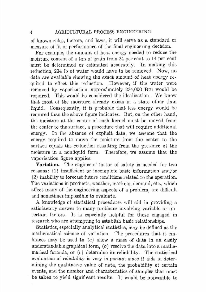
of known rules, factors, and laws, it will serve as a standard ormeasure of fit or performance of the final engineering decision.
For example, Lhe amount of heat energy needed to reduce the
moisture content of a ton of grain from 24 pCI' cent to 14 per cent
must be determined or estimated accurately. In making thisreduction, 234 Ib of water would have to be removed. Now, no
data are available showing the exaet amount of heat energy required to effect this reduction. However, i f the water wereremoved by vaporization, approximately 234,000 Btu woultl be
required. This ,vould be considered the idealization. We know
that most of the moisture already exists in a state other than
liquid. Consequently, it is probable that less energy would be
required than the above figure indicates. But, on the other hanel,
the inoisture at the center of each kernel must be moved from
the center to the surface, a procedure that will require additional
energy. In the absence of explicit data, we assume that the
energy required to move the moisture from the cente!' to the
surface cquals the reduction resulting from the presence of the
moisture in n nonliquid form. Therefore, we assume that thevaporization figure applies.
Variation. The engineers' factor of safety is needed fur two
reasons: (I) insufficient or incomplete basic information and/or
(2) inability to forecast future conditions related to the operation.
The variations in products, weather, markets, demand, etc., which
affect many of the engineering aspects of a problem, are difficult
and sometimes impossible to evaluate.
A knowledge of statistical procedures will aid in providing asatisfactory answer to many problems involving variable or un
certain factors. It is especially helpful for those engaged in
research who are attempting to establish basic relationships.
Statistics, especially analytical statistics, may be defined as the
mathcmatical science of variation. The procedures that it em
braces may be used to (a) show a mass of datu in an ensily
understandable graphical form, (b) resolve the data into a muthe
matical formula, or (c) determine its reliability. The statistiealevaluation of reliability is very important since it aids in deter
mining the qualitative value of data, the probability of certain
events, and the number and characteristics of samples that must
be taken to yield significant results. I t would be impossible to

7/16/2019 Engenering Agriculture Perry
http://slidepdf.com/reader/full/engenering-agriculture-perry 16/422
THE ENGINEERING APPROACH 5
give the reader a workable knowledge of statistics in a few shorL
paragraphs, but his interest can be excited by the followingexample.
A class of 20 students wtts divided into two scotians of 10
<>tndcnts each who were taught by different instructors. The
final grades [or the two scctions were as tabulated.
Section .1 Section B
78 8200 71i(m 81
77 9784 8487 9989 7396 7872 8654 87
Average 78.7 Average 84.8
The instructor in section A was criticised for doing a poor jobof teaching because (1) the class average was lower than that of
B, (2) the poorest student in A made a lower grade than the
pooref>t student in B, ancl (3) the best student in A had a lower
grade than the best in B.
However, a Btatistical analysis showed the following. The
Htandard deviation, which i . a measure of variation, was found
to be 8.4 for section A and 8.5 for B. This finding indicates that
two-thirds of all the possible grades represented by the samplewould fall within the range defined by the average plus and minus
the standard deviation. In sediol1 A this range would be 70.3-87.1
and in B, 75.8-92.8. Note that of the total range, 70.3-92.8 of
both sections, 75.8-87.1 or 50 per cent of the entire range is
common to both. This indicates that it is possible that the grades
are a chance randomization of a single group rather t.han a result
of pOOl' teaching. A st.andard st.atistical t.est. of significance ap
plying the pooled st.andard deviation, 8.5 and the difference between the averages 5.6, shows that t.here is only one chance out
of 20 that the section difference is due to poor teaching. The
difference between the averages would have to be over 6 before
the statistician would consider the possibility that the result was
a function of difference in teaching ability.

7/16/2019 Engenering Agriculture Perry
http://slidepdf.com/reader/full/engenering-agriculture-perry 17/422
6 AGlUCULTURAL PROCESS ENGINEERING
This simple example demonstrates in an elementary way the
difficulties that may urise when data are taken at face value. The
engineer should be analytically critical of the value of a number
which is an average of a series of observations. What is thc
variation in the observations from which the average is derived?
Is the variation clue to the method of sampling? Are the ob
servations comparable? What causes the individual observations
to be inconsistent? And finally, just how accurate or representa
tive is the average? The standard deviation as noted before is
an index of variation or accuracy. Similar indices are available
for treating a series of comparable averages, for evaluating the fit
of a curve to plotted data or data to a curve, etc.
A useful approximate relationship to remember is that in a
normally distributed sample,
(Range of means) = (Sample range)/VNo. of samples
For example, the percentages of the moisture content of 5 samples
of grain tabn from a field are respectively 11, 17, 15, 15, and 13,
the average being 14.2 pel' cent. The range of the means or range
within which the true average probably exists is
(17-11)/Vs
or 2.68. I f the above 5 samples are true random samples, the
probability is approximately 2: 3 that the true average will fall
between 14.2 ± 2.68/2, or 12.9 to 15.5 per cent.
This statistical discussion is not intended to provide the readerwith a tool for accurate evaluation of a varying situation but is
intended to excite interest and caution and to indicate that factors
that vary considerably may yield finite results when treated
properly.
Economics. The economic phase of an engineering problem
(discussed in detail in Chap. 13) must never be overlooked.
Many engineering processes are designed specially to reduce pro
duction costs, usually by speeding up the process, eliminating 01'making manual labor more efficient, or reducing overhead costs.
A new or improved engineering procedure must always be judged
by its economic value. The effect may be indirect in that a p a r ~ticular machine or operation may contribute to better application
pf !).nother unit,

7/16/2019 Engenering Agriculture Perry
http://slidepdf.com/reader/full/engenering-agriculture-perry 18/422
THE ENGINEERING APPROACH 7
In processing work there is usually a distinct if not small dif
ference between the cost of the raw products and the selling
price. The processing operation must be performed well withinthis economic bracket if a fair return on the investment is to beassured. Economic improvement of an operation is usually pro
duced in one of two ways: by reducing the cost of production per
unit 01' by raising the net return pel' unit. Increased net rcturncould result from reducing the salvage, using the by-productsmore effectively, or raising the quality of the product. Although
the processing engineer may not be conscious of it, his activities
are usually directed toward one of the above mentioned objectives.

7/16/2019 Engenering Agriculture Perry
http://slidepdf.com/reader/full/engenering-agriculture-perry 19/422
CHAPTER 2
Fluid Mechanics
NOMENCLATURE
A_ = area, sq ft
•1/ = wall-effect, factor, d i l l 1 e I l s i o n l l \ s ~ .C = clearance, ft.D = diamet.er.E =0 number of rows of tubes normal to fluid stream.
F = friction loss, ft Ib per lb or ft .
f = cocfficient, dimensionless.
G = flow rate, gal per min.
a = acceleration of gravity, 32.2 ft per SC(:2.
h = height, ft.K. = a proportic)JU1lity constant.
L = depth, ft.
1 = length, ft.
II!, n = exponents.
P = force, lb.
p = pressure, Ib per sq in.
pi = pressure drop, in. of W!lter.
R = hydraulic radius, ft.
Re = Reynolds number, dimensionless.
I = time, sec.V = velocity, ft per unit of Lime.
Yo = air rate, eu ft pel' min Rq ft .
v = void spaco, a decimal.W = work energy, ft Ib per Ib or work head, ft.
w = weight rate, Ib per unit of time.
x = a quantity of fluid, lb.
y = separation distance, ft.
f = roughness factor, dimensionless.
'Y = specific weight, lb pel' eu ft .
Jl. = fluid viscosity, lb per ft sec.J.!.f = fluid viscosity, Ib-seo per ft2.
A complete study of fluid mechanics would be divided into twoparts: fluids at rest 01' hydrostatics and fluids in motion or hydro
dynamics. The first part, that treating of fluids at rest, will be
8

7/16/2019 Engenering Agriculture Perry
http://slidepdf.com/reader/full/engenering-agriculture-perry 20/422
FLUID MECHANICS 9
assumed to have been covered in the required physics, chemistry,or basic-engineering courses. The second part, which deals with
the various facturs affecting the relntionsltip betwecn the rate offlow and the various pressures tending to cause or inhibit flow,
will be treated in detail. More specifically, such things as the
amount of a fluirl, water, air, milk, or brine, e.g., flowing througha system of pipes if the pressure causing the flow is known 01' thepower required to produce a desired mte of ail' flow through grain
which is to be dried will be considered. The individual betors
involve<l will be studied and related to the various fluid-flow all
plications in which the processing engineer iR interested.
BASIC CONSIDERATIONS
2.1. Classification of Fluids. Fluids are classified as either
compressible, gases; or incompressible, liquids. Liquids [Ire compressible to a very small degree, but no significant error results
in most engineering calculations if incompressibility is assumed.
The principles of fluid flow apply equally well in both cases.2.2. Analytical Basis. The analysis of any fluid system must
take into consideration one l l l ' more of the following:
1. Conservation of mass.
2. Conservation of energy.3. Newton's laws of motion.
a. Every body continues in a state of rC'st or of uniform motion in a straight line unless compelled by force to change
that state.I). The rate of change of mumentum is proportional to the
force applied and takes place in the direction of the fOl'ce
application.
r" To every action thero is always an equal and opposite re
action.
The term fluid system as herein considered refers to any part
of a building or unit or series of units of equipment which isrelated to fluid mechanics. It, may be a complete system suchas a water 01' ventilating system for a processing plant or a single
unit such as a valve, filter, pump, or a length of pipe. It musthave definite boundaries. Consider Fig. 2.1. This hydraulic
system consists of a pump, filter, valve, elbow, and connecting

7/16/2019 Engenering Agriculture Perry
http://slidepdf.com/reader/full/engenering-agriculture-perry 21/422
10 AGRICULTURAL PROOESS ENGINEERING
pipe and is only a small part of a complete system. Points A and
B are the boundaries that define the system under eonsideration.
The simplest case is based on the assumption that all conditionsare constant with time at each point in the system. Fluids fre
quently flow with an irregular rate, that is, surge, under certainconditions. Situations where this condition must be recognized
are few.I f the rate of flow is constant at any point and there is no
accumulation or depletion of fluid within the system, the mass
rate of flow at any number of points within the system must be
constant since lU!.tter can be neither created nor destroyed. Themathematical statement of this follows:
A1Vl'Y1 = AZVZ'Y2 = .. . = AnVn'Yn = W (2.1)
where A = cross-sectional area of conduit, sq ft.V = linear velocity of fluid, ft per sec.
y = specific weight, Ib per cu ft.w = weight of material flowing, Ib per sec.
In engineering, a four-dimensional system including force, mass, length,and time is most generally used. The pound is used for the unit of mass(quantity of matter). The pound is also used for the unit of force. Thispractice has developed because the quanti!;y of matter is measured by observing the force which is exerted on a balance or scale. Thus when wespeak of weight, we commonly refer to the mass (quantity of matter) ratherthan the force (earth-pull) which actuates the scales.
In general, force is proportional to the product of mass and aCCelFlrlltion.In the engineering dimension system, the proportionality constant is
l/g., where go =: 32.17 (lb mass per Ib foree)/Cft per sec2) . Note that thisis not simply g, the gravitational acceleration, which has the dimensions offeet per second squared. Thus
Throughout the text, the expression ma8S is intentionally avoided becauseof its common connotation wig, that is, Weight/Gravitational a c c e l ~ r a t i o n .The variation of weight of a given quantity of matter with geographicallocation is so small as to be ovedooked in agricultural processing. When
weight (strictly speaking, earth pull) is used to designate quantity of matter, one unconsciously multiplies by (pounds of matter per pound of weight).In using weight, tlie relation between force and mass becomes
F = w(lb mass per Ib force)a = ~go g

7/16/2019 Engenering Agriculture Perry
http://slidepdf.com/reader/full/engenering-agriculture-perry 22/422
FLUID MECHANI(;S 11
Example. Water is flowing in [I pipe 6 in. in iill,ide riiametcr at a velocity
of 60 ft per min. The pipe enlarges to 12 in. in diameter. What is the
velocity in the larger section and the quantity flowing?
Weight rate of flow = Arca X Velocity X Lb PPI' eu ft = w
= '11'Cf2)2 X !lO X 62.4 = 73!l III pOl' min
The velocity in the larger section
73()
= ' ) 'XA
736 .----R 2 = 15 ft pe r nl l l l62.4 X '11'(T'x)
(Note that fo!' liquids am\ g a ~ ( ' s , where thf' nhange in dpTlHit,y is llegligihl(', the
velocity varicR invel'sf'ly as the squal'e of the diameter.)
A useful equation is
V = U.5G/D 2
in which V = velocity, ft per min.G = quantity flowing, gal per min.D = pipe diameter, in.
(2.2)
Likewise, since energy can be neither created nor destroyed,
the total energy represented at one point in the system must
equal that at any other point plus intervening transfers. This
condition is the basis of all hydrodynamic calculations and will
be treated in considerable detail.
MECHANICAL ENERGY BALANCE
Consider the hydraulic system shown in Fig. 2.1 located above
a reference plane which might be represented by a level floor and
which is defined as existing between points A and B. The total
mechanical energy involved in this or any other system is made
up of three elements.1. Energy available because of elevation above a referenceplane.
2, Energy available because of internal pressure.
3. Energy available from the moving fluid.

7/16/2019 Engenering Agriculture Perry
http://slidepdf.com/reader/full/engenering-agriculture-perry 23/422
12 AGRICULTURAL PROCF,SS ENGINEERING
Filter
Reference plane
Fig 2.1. A hydraulic system.
2.3. Elevation Energy. A quantity of fluid of weight x is
considered flowing through the system. At point A it has a
potential or elevation energy value of
(2.3)
in which x = lb of fluid.hi = distance above reference plane, ft.
I f the unit of fluid under consideration is released and is permittedto fall or move from its initial position to the reference plane, it
has the ability to do an amount of work equal to xh; or, anamount of work equal to xh would be required to lift it from the
reference plane to a point h ft above the plane.
2.4. Pressure Energy. The fluid at point .Ii is subjected toan internal static pressure of p expressed in Ib per sq in. Thisis in addition to the energy resulting from elevation xh and may
result from a pump, elevated supply tank or other source. Aquantity of potential energy exists since the.x quantity of fluidmust be moved past point A against this pressure. I f released,

7/16/2019 Engenering Agriculture Perry
http://slidepdf.com/reader/full/engenering-agriculture-perry 24/422
FLUID MECHANICS 13
this energy is availaLle to do work that would be defined in termsof force and distance tlms:
The distance through which the force acts is,
xhA
A being the area of the conduit in square feet. The force is the
unit pressnre times the area 01'
The potentia'! energy is thr product of the force times the dis
tance, or(2.4)
where ]J = pressure, Ib per 1)[1 in.'Y = specifiC' weight, Ib per ell ft.
2.5. Velocity Energy. A body in motion possesses an amountof kinetic energy which in this case is equal to
x(V2 /2g) (2.5)
where V = lineal' velocity, ft per sec.g = acceleration of gravity, 32.2 ft pel' sec2
•
Becau::,e of this motion, the quantity of fluid under considerationif brought to rest is able to do an amount of work equal to equation 2.5, or, conversely, the same amount of work is required to
bring the fluid fro111 zero to V velocity.
2.6. Total Hydraulic Energy. The sum of the three types ofenergy present at A, equations 2.3, 2.4, 2.5, is the total mechanicalenergy available at A. This energy plus the energy W supplied
by the pump less that lost because of fluid friction F in the pipes,
joints, etc., must equal that present at point B because of the
conservation of energy. This sum is:
Since x is common to all terms, it cancels, and the final equation is

7/16/2019 Engenering Agriculture Perry
http://slidepdf.com/reader/full/engenering-agriculture-perry 25/422
16 AGRICULTURAL PROCESS ENGINEERING
2.7. Stl'eamlined and Turlmlent Flow. In streamlined flow
the fluid moves in parallel elements, the direction of inotion of
each element being parallel to that of any other element. Thevelocity of any element is constant but not necessarily the same
as that of an adjacent clement.
In turbulent flow the fluid moves in elemental swirls or cc[ches,
both velocity and direction of each element changing with time.
A violent mixing results, whereas there is no significant mixing in
the case of streamlined flow.
2.8. Distribution of Velocities. A velocity traverse of a fluid
(liquid or gas) flowing in a pipe will show that the velocity is
o 100%
Streamlined
Streamlined
o 100%
Turbulent
Fig. 2.2. Streamlined and turbulent flow.
highest at the center and decreases toward the surface of the con
tainer, the velocity at the surface being zero. This characteristic,
which holds for both streamlined and turbulent flow, is shown inFig. 2.2.

7/16/2019 Engenering Agriculture Perry
http://slidepdf.com/reader/full/engenering-agriculture-perry 26/422
FLUID MECHANICS 17
The velocity gradient for streamlined flow in a long circular
conduit is parabolic in shape; and the a,'erage velocity is onehnlf t.he maximum, which is at the ccnter. For turbulent flow, the
gradient finUcns and the relationship between the maximum Hnd
average veloeity chango::;, its exact value beillp; a function or a
number of conditions under which flow resultR.
2.9. Reynolds Number. Reynolds, an English i n v e ~ t i g a t o rwho was the first to demonstrate the finite cxiiitelH'C of strcal11-
Fig. 2.8. Rf'ynol(ls dcvie!) for studying til(' transition frolll Btrcumlincd to
turbulent flow.
lined and turbulent flow, developed the mathematical relatiol1::;hip
defining the conditions at which fiow change:'! from stl'eamlined to
turbulent. Reynolds introduced a thin stream of colored liquid
into the bell inlet of a pipe as shown in Fig. 2.3. He found that
the colored thread persisted under low velocities but as t.he
velocity was increased there was a definite point at which the
thread broke and the coloring filled the tube due to eddies or
turbulent flow. The velocity at which transition results is called
the criticaL velocity. Reynolds found there were four factors that
affect the critical velocity. These faetorR and their mathemaUcal
rdatinnship follow:
Re = DV'YIf.!.
where Re = Reynolds number, dimensionlcsH.D = inside diameter of pipe, ft.
V = average velocity, ft per ser.'Y = specific weight, Ib per cu ft.J.L = Huid viscosity, lb per ft sec.
(2.8)
7/16/2019 Engenering Agriculture Perry
http://slidepdf.com/reader/full/engenering-agriculture-perry 27/422
18 AGRICULTURAL PROCESS ENGINEERING
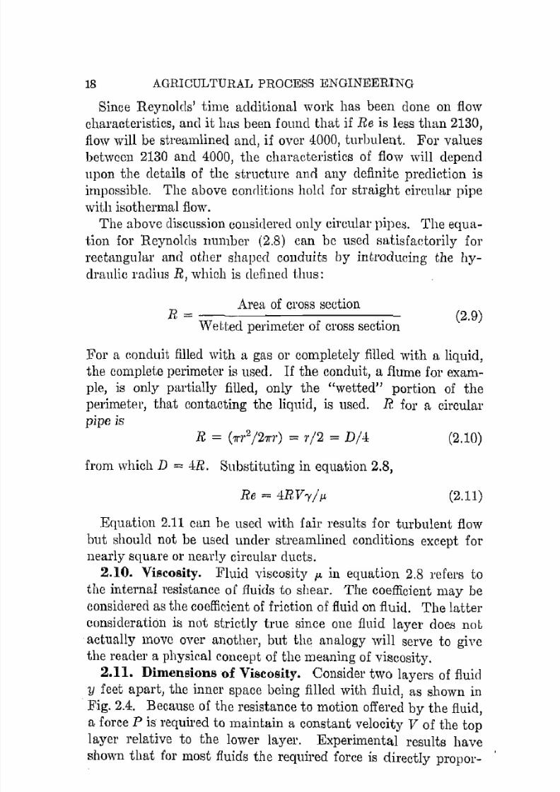
Since Reynolds' time additional work has been done on flow
characteristics, and it has been found that if Re is less than 2130,
flow will be streamlined and, if over 4000, turbulent. For valuesbetween 2130 and 4000, the characteristics of flow will depend
upon the details of the structure ano any definite prediction is
impossible. The above conrlitions hold for straight circular pipe
with isothermal flow.
The above discussion considered only circular pipes. The equa
tion for Reynolds IlUlllber (2.8) can bc used satisfaetorily for
rectangular and other shaped conduits by introducing the hy
draulic radius R, which is defined thus:
Area of cross sectionR = (2.9)
Wetted perimeter of cross section
For a eonduit filled with a gas or completely filled with a liquid,
the complete perimeter is used. I f the conduit, a flume for exam
ple, is only partially filled, only the "wetted" portion of the
perimeter, that contacting the liquid, is used. R for a circularpipe is
R = (71'1'2/271'7') = 7'/2 = D/4 (2.10)
from which D = 4R. Substituting in equation 2.8,
Re = 4RV'yjjj (2.11)
Equation 2.11 can be used with fair results for turbulent flow
but should not be used under streamlined conditions except fornearly square 01' nearly circular ducts.
2.10. Viscosity. Fluid viscosity jJ. in equation 2.8 refers to
the internall'esistanee of fluids to shear. The coefficient may be
considered as the coefficient of friction of fluid on fluid. The latter
consideration is not strictly true since one fluid layer does not
actually move over another, but the analogy will serve to givc
t.he reader a physical concept of the meaning of viscosity.
2.11. Dimensions of Viscosity. Consider two layers of fluidy feet apart, the inner space being filled with fluid, as shown in
Fig. 2.4. Because of the resistance to motion offered by the fluid,
a force P is required to maintain a constant velocity V of the top
layer relative to the lower layer. Experimental results have
shown that for most fluids the required force is directly propol'-

7/16/2019 Engenering Agriculture Perry
http://slidepdf.com/reader/full/engenering-agriculture-perry 28/422
FLUID MECHANICS
L .__======_L_ ::=-,/ Area in sq It
Fig. 2.4. Viscosity clements v i ~ u a l i z e d .
19
tional to the resulting velocity, directly proportional to the area
A, and inversely proportional to the separation distance y. Stated
mathematically, this is
P = N(VA/y) (2.12)
/.If being a (Jollstu,nt of Pl'Opol'tionajity which is the ('oefficient of
viscosity. IJ.j by solution is found to be
Py}.tf = --
VA
where P = force, lb.11 = separation distance, ft.
V = relative velocity, ft pel' sec.A = plate area, sq ft.
Lb-secJl.j will be found to have the dimensions, - -2- '
Ft
(2.13)
I f y, V, and A are considel'ed to have unit values, that is, one, the
viscosity will be numerically equal to P and will have the dimension lb-sec pel' ft2. In engineering the so-called mass viscosity J.I.
is more commonly employed. This is obtained by multiplying
ILl by the force-masH pl'ollOrtionality constant go. Thus I'" = P-Igo
and has the dimensions lb/sec-ft. A list of viscosities that will be
useful in fluid flow calculations will be found in Table 2.1.
Published values of viscosity arc usually in centipois6S (0.01
dyne-sec pel' sq em or 0.01 gm per em-sec), the egs unit of abso
lute viscosjty. They must be converted to the engineering system
of units in order to be used in the equation for determining
Reynolds numbers. Conversion can be made by multiplying
centipoises by 0.000672 which gives the absolute viscosity in terms
of lb per it-sec.

7/16/2019 Engenering Agriculture Perry
http://slidepdf.com/reader/full/engenering-agriculture-perry 29/422
2() AGRICULTURAL PROCESS ENGINEERING
Tahle 2.1 VISCOSITY INDICES FOR VARIOUS MATERIALS
Tem- Vi,cositypera· - - - - _ . _ -lure. {{G. Cellti- Lb per
Material of (,lpprux.) pOi$leR /<"I-Sec
Air 32 0.0171 0.0000115 /ntcrrwtional Criiiwi Tabl"
70 0.0181 0.0000122 International CriiicaI1'ablc.212 0.0218 0.0000147 Internalional Critical TalJlm
Water 32 1.(100 1.793 0.00121 hitenwtiomll Critical Table,
70 o.ons 0.984 O.OOOOo! h,t"nalional Critical Tabl"120 n.987 0.559 0.000375 I"tenlational Critical Tablcs
Sucrose, 2 0 ~ ) flo1. :12 1.081\ 3.818 0.00256 International Critical Taliles
70 1.()82 1.0]6 0.00129 InieniU(iollal Critical TallIes
176 1.0,15 0.502 0.000308 International Critical TaMes
60% '01. 70 1.289 00.2 0.0404 International Critical Tabl"176 L252 5 . 4 ~ 0.00364 International Critical Table.,
Lub. oil, S.A.E. 10 60 0.9 100 0.0672 Mark,' Ilandbook150 0.87 10 0.00672 Mark,' Handiwok
B.A.E.30 60 0.9 400 0.269 Mark.' HandllOok1M (/.87 27 a.(l18.1 iffark,' Handbook
Liquid Ammonia 5 .O. 66 0.25 0.000168 Refriueration Data Bool,80 0.60 0.21 0.000141 Refriueration Data Book
Freon-12 5 1.44 0.33 0.000222 Refriaeration Data Book80 1.30 0.26 0.000175 Refriueration Data Bouk
eaCh brine, 24% sol. -10 1.238 12.5 0.00840 Re/rioeration Data Book
0 1.234 8.8 0.00501 Refriaeration Data Book35 1.227 3.7 0,00248 Refrioeration Data !Jook
NaCl brine, 22% '01. 0 1.19 0.1 0.00410 Refriaeration Data Book35 1.17 2.7 0.00181 Re/riaeration Data Book
Molasses, heavy dark 70 1.43 6600 4.43 Gould', PumpS100 1.38 1872 1.26 GOUld', Pump.120 1.31 920 0.618 Gould', Pump'150 1.16 374 0.251 Gould', Pump.
Soybean oil B6 0.92 40.6 0.0273 EshbachOlive oil 86 0.92 84,0 0.0665 EshbachCotton-seed oil 60 0.92 91.0 0.061 'EshbachMilk, whole 32 1.036 4.28 0.00288 Rogers et at.
68.4 1.03 2.12 0.00143 Rogers ct at.Milk,skim 77 1.04 1.37 0.000922 Bateman and SharpCream, pasteurized, 20% Cat 87.4 1.01 6.20 0.00416 Dahlberg and Helling
30% Cat 37.4 1.00 13.78 D.0093(; Dahlberg and Helling
Viscosity is usually measured by a Saybolt viscometer. The
time in seconds is noted for a specified quantity of fluid to flow
through a short tube of small bore under preseribed head and
temperature condition. The viscosity is reported in seconds.
The Saybolt Universal viscometer is used for fluids of light tomedium viscosity. The Saybolt Fural has a tube of larger boreand is used for heavier fluids.
Viscosities in centipoises can be found from Saybolt Universal
seconds t by the following equations:

7/16/2019 Engenering Agriculture Perry
http://slidepdf.com/reader/full/engenering-agriculture-perry 30/422
FLUID MECHANICS 21
, " ( 195)entlpOlses = 0.220[ - i-- fl.G. (2.1..Jo)
when t varics from 32 to 100 see
( 135)= O.220t - - t- B.G. (2.15)
when t is greatC'l" than 100 see
Conversion from Sayholt Fuml seconds ill made tIm,;:
(:entipoiHPi'i = (2.24t _ 1 ~ ! . ) S.G. (2.1 Ii)
When t varies from 25 to 40 see
( 00)= 2.1 (1t - I S.G. (2.17)
When) greater than --10 sec
The critical velocity, that is, the velo<?ity below whi.ch stream
lined flow exists (He = 2130), is plotted against diameter of pipefor air and water at two tcmperatures in Fig. 2.5. Note that the
700I
\ \II
I
\ \II
600
I
' \f\I
I
\ ~III
\\ 1"'- "'"\
......r--.. ~ -- 1"'--
l \
"' ~ r~ 5 0 ' F
200
100
00 0.2 0.4 0.6 0.8 1.0 1.2 1.4 1.6 1.8 2.0Diameter, feet
Fig. 2.5. Relationship of velocity and pipe diamf'ter for flow at the critical
velocity, Re = 2130.
7/16/2019 Engenering Agriculture Perry
http://slidepdf.com/reader/full/engenering-agriculture-perry 31/422
22 AGRICULTURAL PROCESS ENGINEERING
velocity of air increases with temperature but that of water de
creases owing to the fact that the viscosity of gases JL increases
with temperature but that of liquids decreases. This shows thatif turbulent flow is required, heat-exchanger design, e.g., small
pipes are not to be desired.
FRICTION LOSSES
The P 01' friction head loss term in the Bernoulli equation (2.7)
represents energy lost or dissipated because of internal fluid re
sistance, excess turbulence, or resistance of the inner surface ofthe l'etainer to flow. EVl1.1uation of this fuctor involves the
Reynolds number, the dimensions of the conduit under considera
tion, and certain empiriwl data.2.12. Darcy's Formula. One of the most widely used formu
las for determining the friction loss was developed by Darcy,
F "'" !(Z/D) (V2/2g)
where l = length of pipe, ft.D == pipe diameter, it.V = linear velocity, ft per sec.
(f :! acceleration of gravity, 32.2 ft per see.
f = coefficient, dimensionless.
(2.18)
The coefficient f is closely related to Reynolds number Re, but the
relationship is not clefmite enol1gh for general use in a mathe
matical form.
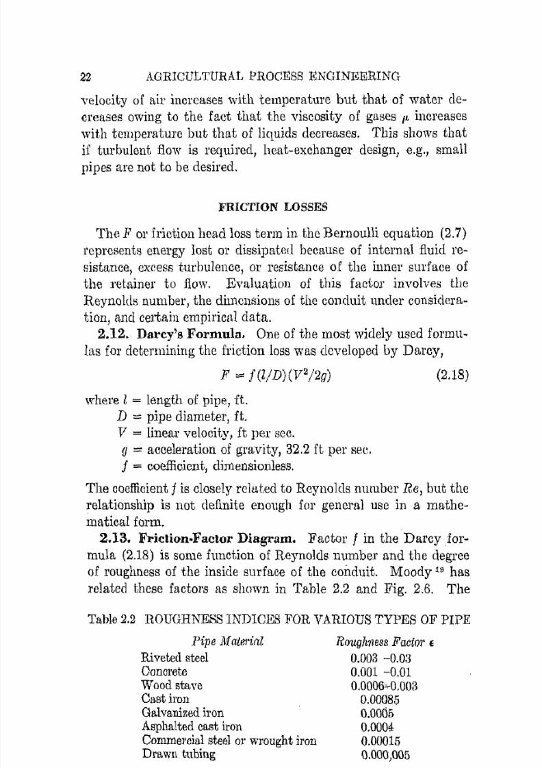
2.13. Friction·Factor Diagram. Factor f in the Darcy formula (2.18) is some function of Reynolds number and the degreeof roughness of the inside surface of the conduit. Moody 19 has
related these factors as shown in Table 2.2 and Fig. 2.6. The
Table 2.2 ROUGHNESS INDICES FOR VARIOUS TYPES OF PIPE
Pipe Mate:rial
Riveted steel
ConcreteWood staveCast ironGalvanized ironAsphalted cast ironCommercial steel 0)' wrought ironDrawn tubing
Roughness Factor E
0.003 -o.oa
0.001 -0.010.0006"-0.003
0.000850.00050.00040.000150.000,005

7/16/2019 Engenering Agriculture Perry
http://slidepdf.com/reader/full/engenering-agriculture-perry 32/422
FLurn M ] ~ C H A N I C 8
".
o.....iOO

7/16/2019 Engenering Agriculture Perry
http://slidepdf.com/reader/full/engenering-agriculture-perry 33/422
2,1 AGRICULTURAL PROCESS ENGINEERING
relative roughness factor is the roughness factor f divided by the
pipe diameter in feet. The relative roughness factor for a particular pipe is referred to in Fig. 2.6 and identifies the curve to be
llsed for selecting a satisfactory f value.For example, a 3-in. (inside diameter) commercial steel pipe
has a relative roughness of 0.0006. This value identifies the
proper curve to be used in Fig. 2.6. I f Reynolds number is found
to be 9 X 10\ the friction factor f is 0.021. Friction factors forwater and atmospheric air can be determined from the values of
VD from the top of Fig. 2.6. Air is flowing at 900 ft per min in
a 20-in. galvanized iron pipe. The relative roughness is 0.003,which identifies the propel' curve of Fig. 2.6. The product of VD
is 300, which provides a friction factor f of 0.027. If Reynoldsnumber is desired, it can be read directly from the VD position.
I t is 1.4 X 10⁵ in this case.
Note that the velocity term V shows in the formula for determining Reynolds number (2.8), in Darcy's formula (2.18), and
in the Bernoulli formula (2.7). Solution of a problem in which
the velocity is known is a straightforward arithmetical procedure.
On the other hand, if velocity is to be determined, solution must
be by trial and error or by a graphical procedure. Trial-and-error
solutions are usually satisfactory, but the graphical method gives
more accurate results. This method is demonstrated by the fol
lowing example.
Example. How many gallons of water per minute will flow through 150
it. of 2-in. pipe under a 15-ft head?The Bernoulli factors that apply are,
and sincehI - F = 1l2j2g
F = jCljD)(V2j2g)
hi - f(ljD)(V2/2g) == V2j2g
Substituting known values and solving,
150 V2 V 2
15 -j-- = - and-fi 64.4 64.4 V2
15 -14fV 2 =-64.4
Transpose anel divide to place f and V2 on opposite sides of the equal sign andeqnate both to a variable thus:
14f = (15/V2) - (lj64.4) "" C

7/16/2019 Engenering Agriculture Perry
http://slidepdf.com/reader/full/engenering-agriculture-perry 34/422
FLUID MECHANICS 25
Plot the two e < t u a t i o n ~l..J.f = C and (15/V2) - (l/M.·!) = C
for a number of values of V. The poinL at which the Cllrves intersect is
the solution (sec Fig. 2.7). This proceduro is known as Newton's method
of solution and can be used to solve many algebraic equations which cannotbe easily solved by other methods.
9
8n
7
5
3
2
o0.2
[\
\
~ N _L::c2 64.4
I'.............
'"
4f =\.
0.4 0.6 0.8 1.0 1.2cFig. 2.7. Graphical solution of velocity problem.
2.14. Resistance of Fittings. Pipe and conduit fittings, be
cause of restrictions to flow, sharp projections, abrupt change in

7/16/2019 Engenering Agriculture Perry
http://slidepdf.com/reader/full/engenering-agriculture-perry 35/422
26 AGlUCULTURAL PROCESS ENGINEERING
shave and dimensions, etc., may (muse [L significant loss of energy
which further adds to the F factor of the Bernoulli equation.
The characteristics of this loss have not been sufficiently ration
alized for mathematical treatment. Considerahle empirical data
are available and, although incomplete as regards many fittings
and fluids, are sufficiently accurate for most design work.
The data are usually presented in one of two ways, either as
loss in pressurc head as a decimal of V2/2g or as an equivalent
length of pipe. Resistance data for a numbcr of fittings expressed
as a fraction of the velocity arc tabulated in Table 2.3. The re-
Table 2.:1 FRICTION LOSS :FACTORS K
Nature of resistance
Valves, fully open
Elbows ({{:.B~ D A D
Tees
x
Discharge nozzles
B
Gateglobeangle
u...&_B_ _ --II: '= b i : ~Ring Spraylain
Entrances
~ -~ A
'Varies, use manufacturers values.
1,
0.157.54.0
A,0.50B,0.25
C, 1.50(a)2D, 1.2596
XA,1.50XB,0.50
A, 0.01 -0.03B,0.01-0.04-C'
A, 0.50B. 0.05C, 1.00
DlK
/J2
0.1 0.3620.3 0.3080.5 0.2210.7 0.1050.9 0.015
(V1-V2 )2
2g

7/16/2019 Engenering Agriculture Perry
http://slidepdf.com/reader/full/engenering-agriculture-perry 36/422
FLUID MECHANICS 27
sistance expressed as an equivalent length of tltraight pipe in
terms of pipe diameter is 40K. For example, a common elbow
C with a J ( of 1.50 would have the sanw l · p ~ i R t D . n e e or produce the
sallle pressure drop as l \ length ()f connecting pipe equal to 1.5
times 40 or 60 clialMi e1's. I t i/'i frequently convenient to use this
equality ill dptE'rmining prC'HS1IJ"P 10RSE'S in lines thai i11('I1111(' vari
ous fittingH.
2.15. Energy Loss('s Due to Sudden Velocity Changes.
When a fluid flowing in a pipe is forced to change velocity, a
certain amount of energy is lost as heat energy because of turbu
lence and work energy due to localized velocity variation. A
list of conditionK in which this combined effect i:; important and
methods used for its determination are given in Table 2.3. Except
for the enlargemcnt conrlition, the IORK factor I{ has bc('J1 deter
mined experimentally.
The loss factors for sudden ('ontnwtion, /:dml'p-rdgcd entrances,
amI nozzles involve two phenomena: turbulence, which has been
discussed, amI stream contraction. Because of incrtia, an element
of fluid does not necessarily follow the wallR of the retainingstructure. For cxample, the :--.troam of water after leaving the
point of sudden contraction in Table 2.3 i.s smaller in diameter
than the pipe and has a velocity higher than it has farther along
in the 11ipe. The point at which this fMeam diameter is n mini
mum is called the vena-contracta. Vigorous turbulence in the
region of the vena-contracta between the wall of the pipe and
the flowing stream, i.e., when there are no reverse eddies, causes
eonsirlerable energy loss. A rounded approach avoids the formation of a vena-contracta, and a cone of expansion with a slope
angle of 7 degrees or less permits a change in velocity with a
minimum energy 10tis. For a detailerl study of these losses, the
reader should refer to a textbook on flui(l mechanics 01' to detailed
H1X'eialized reports.
2.16. Pressure Drop in Heat Exchangers. The resistance
to ail' flow or pressure drop through heat exchangers is important
in such installations as refrigeration plants, air conditioning nnits,driers, etc. In general, it is expedient to use the pressure-drop
data supplied by the manufacturer for the exchanger in question.
A general method of calculating this effect for certain conditions
will be found useful and follows.

7/16/2019 Engenering Agriculture Perry
http://slidepdf.com/reader/full/engenering-agriculture-perry 37/422
28 AGRICULTURAL PROCESS ENGINEERING
Fig. 2.8. Cross section of a heat exehangp.l'.
I f the exchanger is made of a scries of parallel tubes, the pres
sure drop through it can be calculated by thc following equations,
which are the results of studies by a number of investigators.2o
The formulas which should be referred to Fig. 2.8 follow.
,1jEry y2p=
2g
f = 0.75 (C:I')-0.2
where p = pressure drop, lb per sq ft.
E = number of rows of tubes normal to fluid stream.
I' = fluid specific weight, Ib per cu ft.
(2.19)
(2.20)
V = maximum velocity through the minimum cross section,
it pel' sec.
C = clearance between tubes in a row, A-D in Fig. 2.8, ft.
J.I. = viscosity, lb per ft-sec.
Equation 2.19 is probably reliable to within 25 per cent for
pitch distances A of 1.25 to 1.50 tube diameters, which is the
normal commercial spacing. Flow is probably turbulent if
(A-D) Vy/,u i.s greater than 40.
Baffled or finned exchangers require an involved mcthod of cal
culation and will not be discussed here.
2.17. Pressure Drop through Agricultural Products. Ventilating, drying, and dehydrating of agricultural products usually
involve forcing air through a mass of the product. The relation
ship of the rate of flow through the mass to the depth of material
or distance of air travel and the pressure drop through the ma
terial is important since the power requirement, fan or blower

7/16/2019 Engenering Agriculture Perry
http://slidepdf.com/reader/full/engenering-agriculture-perry 38/422
FLUID MECHANICS 29
selection, and drying characteristics are directly related to the::;c.
The calculation of fan or blower requirements and drying char
acteristics are treated in Chaps. 5 and 11, respectively.Consirlerable work has been (lone on the characteristics of
fluid flow through soils and through granular and other material
related to chemical engineering. Unfortunately, these procenures
have not been verified for ul1plication to agricnltural products.
Althuugh some work has been clone toward rationalization of the
rosistance relationships, current usable data are mostly empiricalin nature.
The resistance of a material to air flow is some function of thesurface characteristics and the size and shape of the voids. Con
sider the variations in these factors if we attempt to compare
such agricultural commodities as flax seed, ear corn, walnuts, beeL
seed, oats, and hay. These factors plus natural biological varia
tion due to moisture content, varieties, seasons, and geography
thus far have complicated the complete rationalization of re
sistance data.
Chilton anrl Colburn (Ind. and EnU7". Chem. 23 :913-919. 1931) correlatedthe available resistance data for many uniform granular solid particles usedin chemical-engineering porous beds by means of a lUodified Reynoldsnumber:
Rem = DpVor60",
where Dp = nominal particle diameter, f t .
Vo = air velocity, cu ft per min sq ft.
'\' = fluid specific weight, lb per eu ft.'" = viscosity, Ib pfr ft sec.
The modified Reynolds number was plotted against the friction factor f,in a manner comparable to Fig. 2.6. Although there was no distinct breakbetween turbulent and laminar flow, turbulent flow seemed to persist abovean Re,,,, of 100 and a laminar flow below 20. A single break point could beindicated at Rem = 40. The analysis also showed the following relationshipfor pressure drop through the material:
For laminar flow:
For turbulent flow:
7/16/2019 Engenering Agriculture Perry
http://slidepdf.com/reader/full/engenering-agriculture-perry 39/422
30 AGRICULTURAL PROCESS ENGINEERING
where p' = pressure drop through the nmss, in. WItter.
L = mass depth, ft.
1(" l{ 2 = proportionality constants.Ai = wall effect fact.or, dimensionless (this factur will equal one for
most agricultural installations).
This treat.ment of itself cannot determine resistance data for a particular
agricultural material. I t can be used, however, for evaluating observed data
and determining the limits to which observed dat.a can be extrapolated.
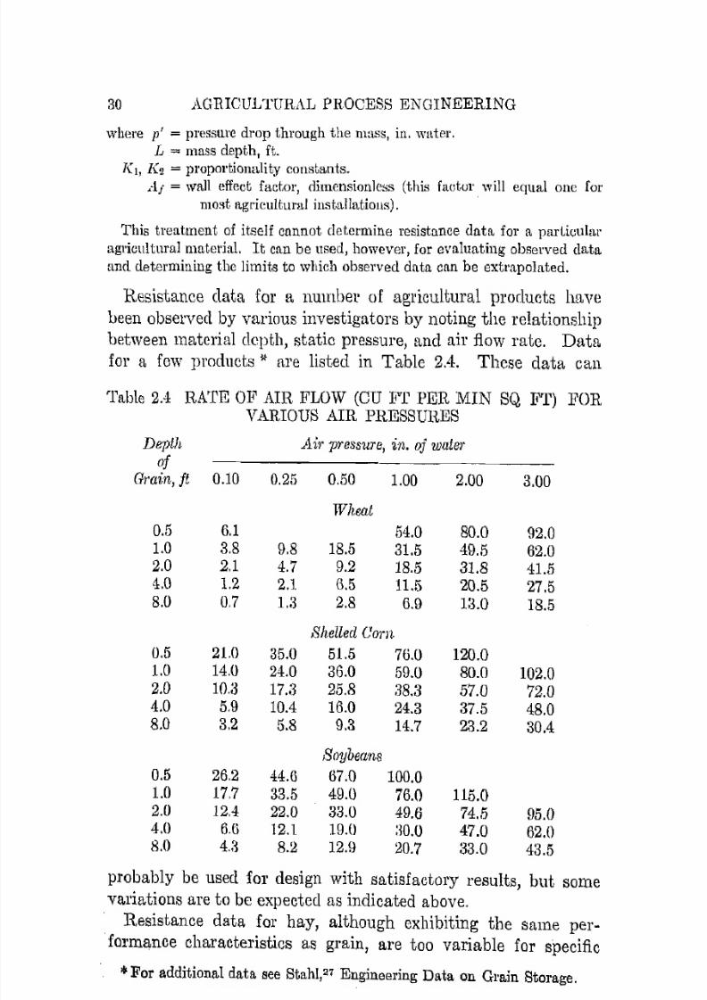
Resistance data for a number of agricultural products have
heen observed by various investigators by noting the relationship
between material depth, static pressure, and air flow rate. Data
for a few products * are listed in Table 2.4. These data can
Table 2.4 RATE OF AIR FLOW (CU FT PER MIN SQ FT)VARIOUS AIR PRESSURES
FOR
Depth Jii1' pressure, in. of waterof
Grain, jt 0.10 0.25 0.50 1.00 2.00 3.00
Wheat
0.5 6.1 54.0 80.0 92.01.0 3.8 9.8 18.5 31.5 49.5 62.02.0 2.1 4.7 9.2 18.5 31.8 41.54.0 1.2 2.1 6.5 11.5 20.5 27.58.0 0.7 La 2.8 6.9 13.0 18.5
Shelled Corn
0.5 21.0 35.0 51.5 76.0 120.01.0 14.0 24.0 36.0 59.0 80.0 102.02.0 10.3 17.:3 25.8 38.3 57.0 72.04.0 5.9 10.4 16.0 24.3 37.5 48.08.0 3.2 5.8 9.3 14.7 23.2 30.4
Soybeans0.5 26.2 44.6 67.0 100.01.0 17.7 33.5 49.0 76.0 115.02.0 12.4 22.0 33.0 49.6 74)5 95.04.0 6.G 12.1 19.0 :lD.O 47.0 62.08.0 4.a 8.2 12.H 20.7 83.0 43.5
probably be used for design with satisfactory results, but somevariations are to be expected as indicated above.
R.esistance data for hay, although exhibiting the same per-
fOl'mance characteristics as grain, are too variable for specific
* or additional data see Stahl,21 Engineering Data on Grain Storage.

7/16/2019 Engenering Agriculture Perry
http://slidepdf.com/reader/full/engenering-agriculture-perry 40/422
FLUID MECHANICR 31
recommendation. Schaller et al,23 recommend that, for hay d r y ~ing, a total pressure drop of 0.75 in. of water be used in selecting
a fan for hay 15 ft deep. For depths of 6 to 8 ft of hay a pressuredrop of 0.5 to 0.6 in. may be userl. The rate of air flow shouldnot be less than 10 ell ft, pel' sq Ii, pel' min. A higher rate ispreferablc.
An acceptable mathematical relntiollHhip of thc variables is:
pi = EYu"'Ln (2.21 )
where Vo = rate of ail' flow, w ft of air at atmosphclic preSHlll'£',
and temperature pel' sq ft of floor area per min.Note that the linear rate through the mass would
he Vo divided by the porosity of the mass.l( = a constant that depends upon the characteristics of
the materbl.pi = pressure drop through the mass, in. of water.
rn = an exponent that varies from material to materialand varies somewhat with depth for anyone mate
rial. Observed values vary from 1.1 to 2.0 approximately with a value of about 1.5 being an
indicated mean.T.1 = depth of material, or distance of air movement
through mass, ft.n = an exponent that varies from 1.0 to 1.1, approxi-
mately.
Note that the pressure drop (head loss) is indicated in inches of
water. To convert inches of water to pounds per square inchmultiply by 0.0362.
I f nand rn were 1.0 and 2.0 respectively, equation 2.21 would
become(2.22)
which is essentially the Darcy friction formula. Now if the exponent of Vo were 1, flow would be streamlined. Since the actual
observed exponents or values of nand m are such that the exponent of Vo in equation 2.21 is bctween 1 and 2, the flow is
probably a combination of streamlined and turbulent. Further·
more, i f this were the case, material with small void spaces would
have m values approaching 1.0. A review of the literature shows
a tendency in this direction.
7/16/2019 Engenering Agriculture Perry
http://slidepdf.com/reader/full/engenering-agriculture-perry 41/422
32 AGRICULTURAL PROCESS ENGINEERING
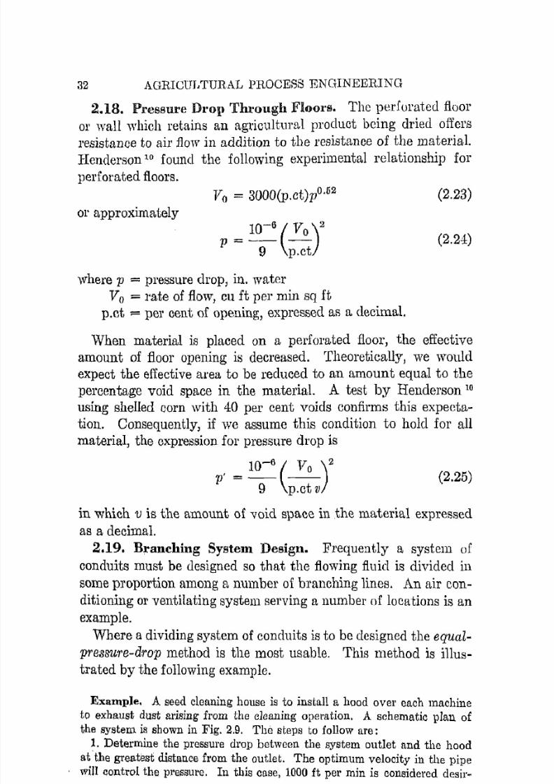
2.18. Pressure Droll Through Floors. The perforated floor
or wall which retains an agdcultuml product being dried offers
resistance to air flow in addition to the resistance of the material.Henderson lO found the following experilnental relationship for
perforated floors.
Vo = 3000(p.ct)pO.52 (2.23)
or approximately
p = 10-6 ( ~ ) 29 p.ct
(2.24)
where p = pressure drop, in. waterVo = rate of flow, cu ft per min sq ft
p.ct ;= per cent of opening, expressed as a decimal.
When material is placed on a perforated floor, the effectiveamount of floor opening is decreased. Theoretically, we wouldexpect the effective area to be reduced to an amount equal to thepercentage void space in the material. A test by Henderson 10
using shelled corn with 40 per cent voids confirms this expectation. Consequently, if we assume this condition to hold for allmaterial, the expression for pressure drop is
p' = 10-6 ( ~ ) 29 p.ct v
(2.25)
in which v is the amount of void space in .the material expressed
as a decimal.
2.19. Branching System Design. Frequently a system ofconduits must be designed so that the flowing fluid is divided in
some proportion among a number of branching lines. An air con
ditioning or ventilating system serving a number of locations is anexample.
Where a dividing system of conduits is to be designed the equal
pressure-drop method is the most usable. This method is illustrated by the following example.
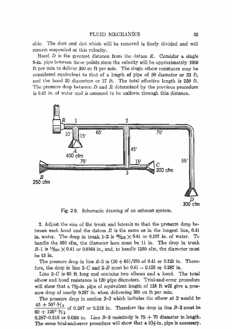
Example. A seed cleaning house is to install a hood over each machineto exhaust dust arising from the cleaning operation. A schematic plan ofthe system is shown in Fig. 2.9. The steps to follow are:
1. Determine the pressure drop between the system outlet and the hood
at the greatest distance from the outlet. The optimum velocity in the pipewill control the pl'eSStll'e. In this case, 1000 it pel' min is considered desir-
7/16/2019 Engenering Agriculture Perry
http://slidepdf.com/reader/full/engenering-agriculture-perry 42/422
FLUID MECHANICS 33
able. The dUAt. and dirt. which will be remand is finely divided and willremain slIspended aI, this velocity.
Hood D is the grcatest distance from the datum R. Consider a single8-in. pipc bptween thf'HO points since the velocity will be approximately 1000
ft pel' min to deliver 300 eu ft pel' min. The single elbow resistance may be
eonsiclered equii'alent to that of a. length of pipe of 50 diameter or 33 ft,flnd the hood 20 diameterR 01' 17 ft. The total effective length is 250 ft.The pressure cit-op hpt.wc[)n D and R dotermined by the previous procedure
is 0.41 in. of water and is assumed to he uuiform through this distance.
2
65' 70'
A 45'
400 efm75' 15' e
3 300 cfmB250 cfm
Fig. 2.9. Schematic drawing of an exhaust system.
55'
D300 efm
2. Adjust the size of the trunk and laterals So that the pressure drop be
tween each hood and the datum R is the same as in the longest line, 0.41in. water, The drop in truuk 1-2 is 61}20o X 0.41 or 0.107 in, of water. To
handle the 850 cfm, the diameter here must be 11 in. The drop in trunk
R-1 is 1%50 X 0.41 or 0.0164 in., and, to handle 1250 cfm, the diameter must
be 13 in.The pressure drop in line R-2 is (10 +65)/250 of 0.41 or 0.123 in. There
fore, the drop in liue 2-C and 2-B must be 0.41 - 0.123 or 0.287 in.
Line 2-C is 60 ft long and contains two elbows and a hood. The total
elbow and hood resistance is 120 pipe diameters. Trial-and-erl'or procedure
will show that a 7*-in. pipe of equivalent length of 135 ft will give a pressure drop of nearly 0.287 in. when delivering 300 eu ft per min.
The pressure drop in section 2-3 which inclUdes tho elbow at 2 would be
45 + 0 7 ' ~ { 2-----"-'- of 0.287 or 0.218 in. Therefore the drop in line B-3 must be60 + 1207
'% 2
0.287-0.218 or 0.059 in. Line B-3 resistively is 75 + 70 diameter in length.The same trial-and-error procedure will show that a 9 ~ - i n . pipe is necessary.

7/16/2019 Engenering Agriculture Perry
http://slidepdf.com/reader/full/engenering-agriculture-perry 43/422
34 AGRICULTURAL PROCESS ENGINEERING
The preRsme drop in R-l is H ) ~ 5 0 of 0.41 or 0.016 in. Therefore, the drop
in I-i1 is 0.41 - 0.016 or 0.394 in. The effect.ive length of I-A is 15 + 70
diameter. Under these conditions and 400 ell ft per min, a 4-in. pipe isadequate.
Line 2-3 is 45 ft long. The pressure drop is 0.218 in., and it c ~ L 1 T i e s 550
ell ft per min. The diameter must be 8 in.
It is advisable to provide dampers or provision for them if needed to bal
ance the system. Certain values, pHrt.icularly hood nnd elbow friction, aresuhject. to variation whi(:h may require adjustment.s after installation.
2.20. Compressihility Error. Air that is subjected to a pres
Iml'e to force it through a series of pipes, a mass of grain, or a
heat exchanger is compressed so that Yl is not equal to Y2. Inmost calculations where drying and ventilation problems arc
being considered, air is assumed to be ineompressible to simplify
calculations, atmospheric pressure being used throughout. Pres
sures under these conditions seldoll) exceed 10 in. of wl1ter and
are usually in the order of 4 or less. The error resulting by
neglecting compression is dependcnt upon the absolute pressures,
I t would be only 2.5 per cent if 10 in. of water were the operating
pressure.2.21. Optimum Rates of Flow. The question frequently
arises as to whether one should have a small pipe or conduit with
high velocity or a large pipe with low velocity. Although each
installation should be analyzed carefully from the standpoint of
initial cost, power requirement, noise level, and operating COtlts,
the following general suggestions can be used as a guide.
Velocities of 4 to 6 ft pel' sec are usually best for water. Ten
feet per second may be used if the system resistanec is low.Where noise is not a problem, ail' systems may be designed for
velocities of 1000 to 1500 i t per min. Velocities up to 2000 i t
pel' min may be used in large pipes.
The reader should realize that these values are general and that
frequently values above or below these should or could be used.
FLOW OF GRANULAR MATERIALS
Grain, ground feed, and other similar materials flow in an entirely different manner than liquids.
2.22. Rate of Flow. Ketchum 15 found that the rate of flow
of wheat from an orifice is independent of the head and varies as
the cube of the orifice diameter. This phenomenon can be ex-
7/16/2019 Engenering Agriculture Perry
http://slidepdf.com/reader/full/engenering-agriculture-perry 44/422
FLUID MECHANICS 35
plainecl in this way: as soon as flow starts, the grain tends to
form a hridge above the orifice. Grain falling from the dome of
the bridge region is replaced by grain from ahove the dome, thegrain above Lhe orifice being discharged first.
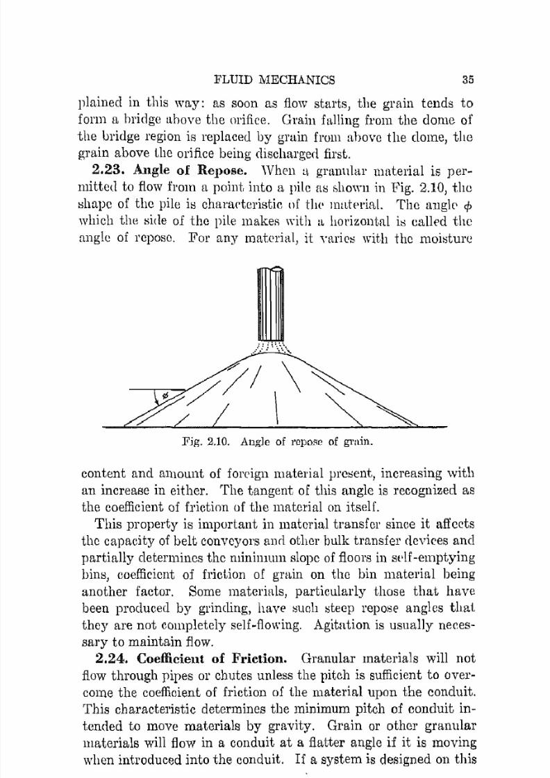
2.23. Angle of Rej)ose. When a granular material is per
mitted to flow from a point into a pile as flhown in Fig. 2.10, the
shape of the pile h; characteristic of til(' material. The angle' cp
which the si<le of the pile makeR with lL horizontal is called the
angle of repose. For any matcri!d, it ,-aries with the moisture
Fig. 2.10. Angle of repo;;e of grnin.
content and alllount of foreign material present, increasing with
an increase in either. The tangent of this angle is recognized as
the coefficient of friction of the material on itself.
This property is important in material transfer since it affects
the capacity of belt conveyors ami other bulk transfer devie'es andpartially determines the minimum slope of floors in sdf-emptying
bins, coefficient of friction of grain on the bin material being
another factor. Some materials, particularly those that havebeen produced by grinding, have l-luch steep repose angles that
they are not completely s e l f ~ f l o w i n g . Agitntion is usually neces
sary to maintain flow.
2.24. Coefficient of Friction. Granular materials will not
flow through pipes or chutes unless the pitch is sufficient to overcome the coefficient of friction of the material upon the conduit.This characteristic determines the minimum pitch of conduit in
tended to move materials by gravity. Grain or other granular
materials will flow in a conduit at a flatter angle if it is moving
when introduced into the conduit. I f a system is designed on this
7/16/2019 Engenering Agriculture Perry
http://slidepdf.com/reader/full/engenering-agriculture-perry 45/422
36 AGRICULTURAL PROCESS ENGINEERING
basis, trouble may arise fr0111 accidental stoppage since starting
flow may be difficult if a minimum pitch is used.
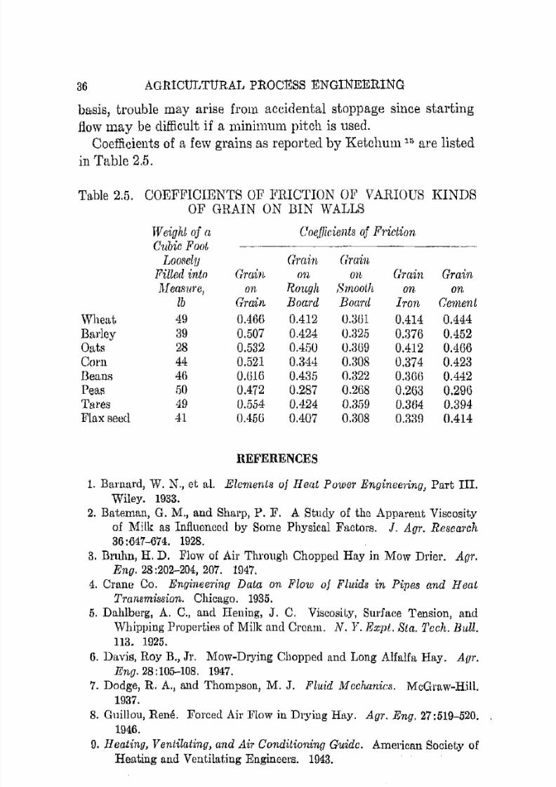
Coefficients of a few grains as reported by Ketchum Hi are listed
in Table 2.5.
Table 2.5. COEFFICIENTS OF FRICTION OF VARIOUS KINDSOF GRAIN ON BIN WALLS
Weight of a Coe.tTlcients oJ FrictionCubic Foot
Loosely Grain Grain
Filled into Gmin on on Grain Grainll-leaslIl"e, on Rough Smooth on on
lb Grain Board Board Iron Cement
Whe:1t 4!) 0.466 0.112 O.3m 0.414 0.444Barley 39 0.507 0.424 0.32,5 0.376 0.'152Oats 28 0.532 0.'150 0.369 0.'112 0.406Corn 4'1 0.521 0.344 0.30S 0.374 0.423Be:1IlS 40 0.616 0.435 0.322 0.306 0.442Peas 50 0.472 0.287 0.268 0.203 0.290Tal'es 49 0.554 0.'124 0.359 0.364 0.394Fbx seed 41 Cl.450 0.107 0.308 0.339 0.414
REFERENCES
1. Barnard, W. N., et a1. Elements of H e ( ~ t Power Engineering, Part III.
Wiley. 1933.
2. Bateman, G. M., and Sharp, P. F. A Study of the Apparent Viscosityof Milk as Influenced by Some Physical Factors. J. Aur. Research36:647-674. 1928.
3. Bruhn, H. D. Flow of Air Through Chopped Hay in Mow Drier. Agr.Eng. 28:202--204, 207. 1947.
4. Crane Co. Engineering Data on Flow of Fluids in Pipes and Heat
TJ'ansmission. Chicago. 1935.
5. Dahlberg, A. C., and Hening, J. C. Viscosity, Surfaee Tension, andWhipping Properties of Milk and Cromn. N. Y. Expt. Sta. Tech. Bltll.
113. 1925.
6. Du.vis, Roy B., Jr. Mow-Drying Cbopped und Long Alfalfa Hay. AUT.
Eng. 28 :105-108. 1947.
7. Dodge, R. A., and Thompson, M. J. Fluid Mechanics. McGraw-Hill.1937.
8. Guillon, Rene. Forced Air Flow in Drying Hay. Agr. Eng. 27:519-520.
1946.
9. Heatin(], Ventilating, and Air Conditioning Guide. American Society ofHeating and Ventilat.ing Engineers. 1943.
7/16/2019 Engenering Agriculture Perry
http://slidepdf.com/reader/full/engenering-agriculture-perry 46/422
FLUID MECHANICH 37
10. Henderson, S. M. Hesistancc of Shelled Corn and Bin Walls to AirFlow. Ag)'. Eng. 24:367-369, SUo 1943.
11. Henderson, S. M. Resistance of Soybeans and Oats in Storage to AirFlow. A Ill'. Eng. 2,15: 127-218. 194.·1.
12. Hendrix, A. T. Air Flow Through Baled Hay. Agr. Eng. 26 :369-371.
1945.
13. Hendrix, A. T. Observlttions on the Resistance of Hay to Ail' Flow.Ag!'. En(l. 27 :209-212. 19-16.
14. Hendrix, A. T. Resistance of Hay to Air Flow. A(I)·. Eng. 26 :369-371.
1945.
15. Ketchum, M. S. The Design of Walls, BillS and Gmin Elevators. ThirdEdilion. McGraw-Hill. 19H1.
16. Kratz, A. P., and Fellows, J. R. Pressnre Losses Resulting from Changesin Cross-Sectional Area in Ail' Ducts. Ill. Eng. Expt. Sta. Bull. 300.
1938.
17. Lansford, W. M. Loss of Head in Flow of Flnids Through VariousTypes of O n e ~ unrl One-HaIf-Inch Valves. Ill. Eng. Expt. Sta. Bull.
340. 1943.
18. Marks, L. S. Mechanical Engineers Handbook. McGraw-Hill. 1941.
19. Moody, L. F. Friction Factors for Pipe Flow. Trans. A.S.M.E. 66 :671-
684. 1944.
20. PelTY, J. H. Chemical Engineers' Handbook. Third Edition. McGrawHill. Hl50.
21. Rogers, L. A. Fttndamcntals of Dairy Science. Second Edition. Reinhold. 1935.
22. Rouse, Hunter. Elementary Mechanics of Fluids. Wiley. 1946.
23. Schaller, J. A., Mitchell, N., Dickerson, W. H., Jr. Barn Driers; Prin
ciples of Design, Installation, and Operation. Tennessee VaJley Au
thority. 1945.
24. Shedd, Claude IC. Resistance of Hay to Air Flow and Its Relation toDesign of Barn Hay-Curing Equipment. Agr. Eng. 27:169-170. 1946.
25. Shedd, Claude K Resistance of Ear Corn to Air Flow. Agr. Eng. 26:19-20, 23. 1945.
26. Spaugh, O. H. Ail' Flow Through Beds of Dehydrated Vegetables.
Food Tech. 2 :33-38. 1948.
27. Stahl, B. M. Engineering Data on Grain Storage. AgT. Eng. Data 1.
American Society of Agricultural Engineers. 1948.
28. Stirniman, E. J., Bodnar, G. P., and Bates, E. N. Tests on Resistanceto the Passage of Air Through Rough Rice in a Deep Bin. Agr. Eng.
12: 145-148. 1931.
29. The Refrigeration Data Book.
The American Society of RefrigerationEngineers. 1936.
30. Vennard, J. K. Elementary Fluid Meohanics. Second Edition. Wiley.
1947.
31. Weaver, John W., Jr., Grinnells, C. D., and Louvcrn, R. L. DryingBaled Hay with Forced Air. Agr. Eng. 28:301-304, 307. 1947.

7/16/2019 Engenering Agriculture Perry
http://slidepdf.com/reader/full/engenering-agriculture-perry 47/422
38 AGRICULTURAL PHOCESS ENGINEER.ING
PROBLEMS
1. Find Reynolds number for milk at 70°F flowing at 20 gal pel' min in
sanitary tubing with l%-in. inside diltmcter. Milk weighs 64.2 lb per
eu ft . What would be the diameter of a tube in whieh strcamlined flow
could be expected?2. A tank it in diameter CD) contains 5 ft of water and is fitted at the
bottom with [ l %-in. globe vah'e. What is the initial rate of discharge?
How long will it take to empty the tank if the valve is completely open?
Note that
~ - 2 g h7rD2
~ j (+ 1 dhdQ = A --dt and that t = - ---_:
K + 1 4A 2U Vh
How long will it tRke if a gate valve is used?
3. Milk is to be lifted 12 ft through 30 it of sanitary pipe that contains 2
elbows. Assuming a pump efficiency of 80 per cent, how much power
will be required to pump at a rate of 60 gal per min if %-in. pipe is used?
I f 1 S - i n . pipe is used?
'1. How much power would be required to pump molasses at 70°F (S.G.,1.43) through the system of problem 3 at a rate of 11,6 gal per min,
assuming a pump efficiency of 70 PCl" cent?
5. Fifteen cubic feet of uir per minute pel' square foot of floor are to be
moved vertically through a crib of shelled corn 5 ft deep. The area of
Lhe floor is 120 sq ft, and the connecting pipe is 12 in. in diameter and
35 it long. What is the power requirement, assuming fan efficiency to
be 75 per cent? I f the diameter of the connecting pipe is increased to18 in., how much power will be required'!
6. Air is flowing through a conduit system at 1400 eu ft per min. An 8-in.
galvanized iron pipe enlarges abruptly to 16 in. The l6-in. section is
20 ft long. I t decreases abruptly at the end of the section to 8 in. indiameter. Would the horsepower roquirement increase or decrease, and
by how much, if the cent.ral section were reduced in diameter to 8 in.?
7. For a specific fluid, it. is convenient to have the friction loss available interms of the mte of flow, say in gallons per minute, and the diameter
in inches. For smooth tubes, in the range of Re fr0111 5000 to 100,000,
the friction factor f, is given by the Blasius equation,
J = O.3Hl/Reo.25
Find the friction cOllstant c in
P 1 = c(gal per min)l,76I (D,)4.75
for a fluid of viscqsity of 20 centipoises and a density of 70 pounds percu ft in smooth tubes of inside diameter D' in.

7/16/2019 Engenering Agriculture Perry
http://slidepdf.com/reader/full/engenering-agriculture-perry 48/422
FLUID MECHANICS 39
s. Determine the sizc of the pipcs required for the instflllation I I I tlipaccompflnying figure.
25 ft 20 ft
L
10ftjn u. ftrmm
1000 cu ftper min
20 ft
15 ft r00 cu ftper min
1000 cu ftper min
II. A Imlk heaier with 6 paR'lPR of n ~ " i n . sHnitary tubing (1.38 ill. ID) is
10 ft long up for testing. ·When 20 gal ]ler min are hf'ing rl£>livcJ'e<i
on a ('old test at 50°F, the hPlg:ht of lllilk in i t pip);OIllPter at lhe inlet
is 8.4 ft . Find i he friction lm·s in fI return bend in e(luivalent velocity
heads; in equivalent pipe diameters.

7/16/2019 Engenering Agriculture Perry
http://slidepdf.com/reader/full/engenering-agriculture-perry 49/422
CHAPTER 3
Fluid-Flow Measurements
NOMENCLATURE
A = cross-sectional area, sq ft.b = gage elevation, ft.
C = a proportionality constant.
cp = specific heat at constant pressure, Btu per Ib 0.F.
AC , !:J.ri = pressure head, in. of mercury.
D = diameter, in.
i:J.D = pressure head, it of mercury.
d =' diameter, in.
H = head, i.e., energy in ft-Ib pOl' Ib of fluid.h =' height, ft.
i =' electrical current, amp.E( =' thermometer factor, dimensionless.
k = a proportionality constant.
m = a ratio.
n '" an area ratio, dimensionless.pg = percentage, a decimal.p = pressure, lb per sq in.
Pi =' pressure, in. of water.Q =' a quantity rate.
R = electricall'osistance, ohms.
t = temperature, OF.t, "" 36.5 degrees minus room temperature, °c.V = velocity, ft per unit of time.w = weight, lb.
Wg = gas rate, Ib per min.
'Y = specific weight, lb per eu ft.o = time, sec.
PRESSURE AND VELOCITY MEASUREMENTS
Accurate and practical methods must be used by the pr()cessing
engineer for determining the pressure and velocity of fluids under
study. Considerable knowledge about this phase of fluid me
chanics is important for the researcher, the designer, the contrac-
40

7/16/2019 Engenering Agriculture Perry
http://slidepdf.com/reader/full/engenering-agriculture-perry 50/422
FLUID-FLOW MEASUREMENTS 41
t.or, t.he operator, and the trouble shooter. Types of equipment
and techniques are diverse, therefore satisfactory selection and
pcrformance can be assured only if the individual is well versedin the various types of equipment and methods of procedure.
Various considerations must be given the selection, installation,
and use of the equipment for a ['Jpecific case. Mobility, accuracy,
constancy of calibration, sensitivity, range of operation, ruggedness, reliability, and longevity all must be considered. In thefollowing sections these points will be clarified relative to the
pressure and flow measurement problems that might confront the
processing engineer.3.1. Pressure Ohservations. The pressure heads represented
by the Bernoulli equation al'e in terms of a column of the fluid
under consideration having a height expressed in feet. In prac
tice, pressures are usually indicated in pounds pel' square inch,inches of mercury, or inches of water. Pounds per square inch
are used for relatively high pressures, inches of water for lowpressures, and inches of mercury for pressures less than atmos
pheric or vacuum. The pressure heads H = 144p/y in the Bernoulli equation (2.7) are in terms of the ft-Ib of energy per pound
of fluid, equivalent to the energy of a column h feet high and
H = h (3.1)
The prei:lsure per square inch is expressed by the following equa
tion:
(3.2)
where p = pressure, Ib pel' sq in.h = pressure head of fluid, ft.'Y = specific weight of fluid, I t per cu ft.
The pressure in inches of water is derived and expressed thus:
12hy
Pm. wakr = 62.4
Similal'ily, the expression in terms of inches of mercury is
12h'YPin. meroury = 847
(3.3)
(3.4)
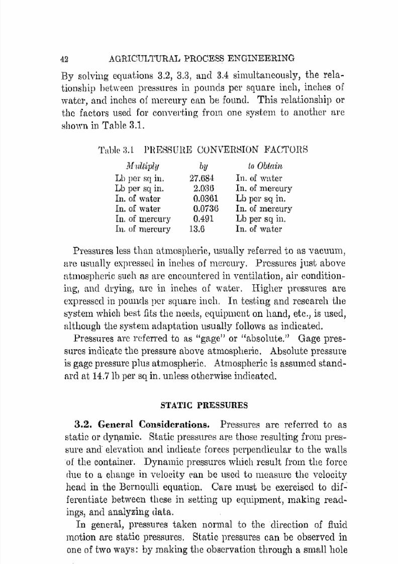
7/16/2019 Engenering Agriculture Perry
http://slidepdf.com/reader/full/engenering-agriculture-perry 51/422
42 AGRICULTURAl, PROCESS ENGINEERING
By solving equations 3.2, 3.3, and 3.4 simultaneously, the rela
tionship between pressures in pounds pel' square inch, inches of
water, and inches of mercury can be found. This relationship ort.hc factors used for cOl1verUng from one system to another are
shown in Tahle 3.1.
Table a.1 PRESSUHE CONVEHSION FACTOHS
Mllltiply
Lh pCI' sq in.Lb per sq in.
In. of w[lterIn. of waterIn. of mercuryIn. of mercury
by
27.6842.0:3B
0.03610.07360.491
13.6
to Obtain
In . of waterIn . of mercury
Lb per sq in.In. of mercuryLb per sq iu.In. of water
Pressures less than atmospheric, usually referred to as vacuum,
are usually expressed in inches of mercury. Pressures just above
atmospheric such as arc cncountered in ventilation, air condition
ing, and drying, are in inehes of water. Higher pressures are
expressed in pounds per square inch. In testing and research the
system which best fits the needs, equipment on hand, etc., is used,
nlthough the system adaptation usually follows as indicated.
Pressures are referred to as "gage" or "absolute." Gage pres
sures indicate the pressure above atmospheric. Absolute pressure
is gage pressure plus atmospheric. Atmospheric is assumed stand
ard at 14.71b per sq in. unless otherwise indicated.
STATIC PRESSURES
3.2. General Considerations. Pl'cs:;ures arc referred to as
static or clyn,amie. Static pressures are those resulting from pres
sure and elevation and indicate forces perpendicular to the walls
of the container. Dynamic pressures which result from the force
due to a change in velocity ('an be used to measure the veloeity
head in the Bernoulli equation. Care must be exercised to dif
ferentiate between these in setting up equipment, making read
ings, and analyzing elata.
In general, pressures taken normal to the direction of fluid
motion are static pressures. Static pressures can be observed in
one of two ways: by making the observation through a small hole
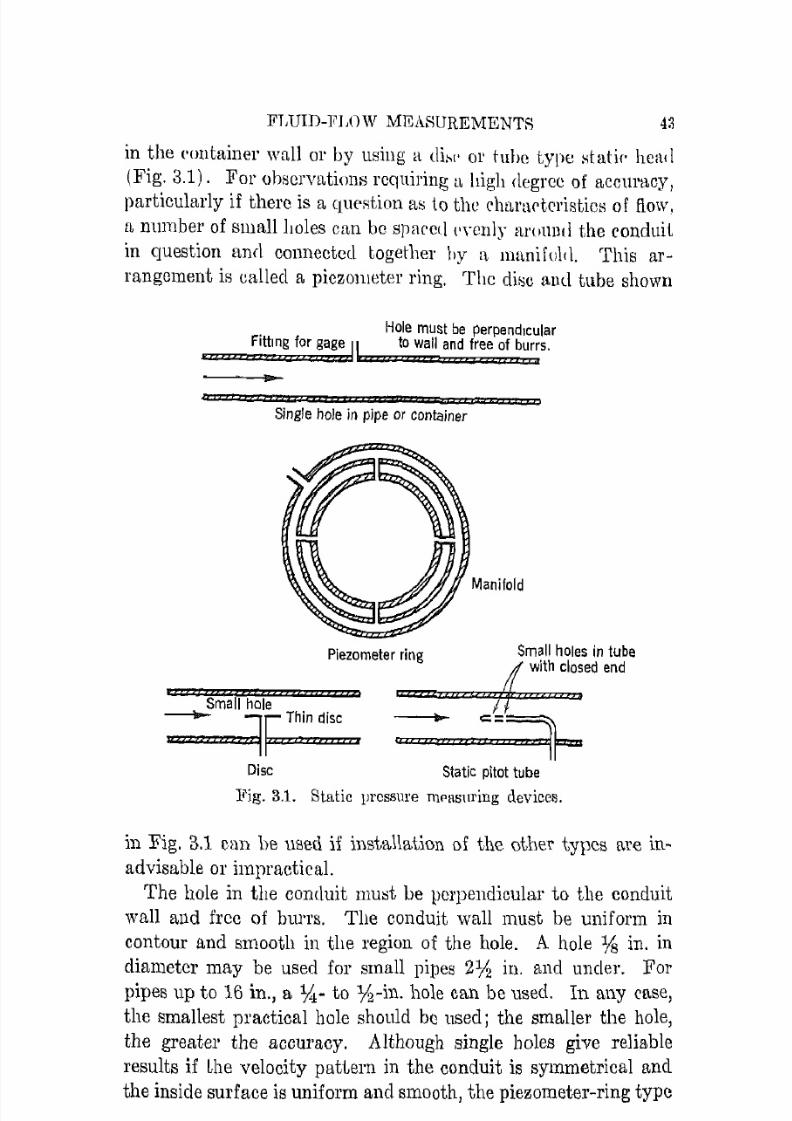
7/16/2019 Engenering Agriculture Perry
http://slidepdf.com/reader/full/engenering-agriculture-perry 52/422
FLUID-FLOW MEASUREMENTS 43
in the ('olltainel' wall 01' by using a d i ~ I ' or tube type Ht uti(' head
(Fig. 3.1). For observations reqniring a high (iegrcc of accuracy,
particularly if there is a qU{,Ation as to the elmrartcristics of flow.
n number of slllall holes can bc spaccd I'Yenly al'utllld the conduit
in question anfl connected Logethel' by a manifold. This ar
rangement is called a piezollleter ring. The disc and tube shown
Fitting for g a ~ ? , l lHole must be perpendicular
to wall and free of burrs.t.
Single hole in pipe or contqiner
Disc Static pitot tube
Iejg. 3.1. Static I11'CS6U1'e fi1pas\lring devices.
in Fig. 3.1 can he llsed 11 im,ta,1!ation of the other types are in"
advisable or impractical.
The hole in the conduit mu::;t be pCl'pendicular to the conduit
wall and free of burrs. The conduit wall must be uniform in
contour and smooth in the region of the hole. A hole lis in. in
diameter may be used for small pipes 2Jf2 in. and uncleI'. For
pipes up to 16 in., a ~ - to %-in. hole can be used. In any case,
the smallest practical hole should be used; the smaller the hole,
the greater the accuracy. Although single holes give reliable
results if Lhe velocity pattern in the conduit is symmetrical ancl
the inside surface is uniform and smooth, the piezometer-ring type

7/16/2019 Engenering Agriculture Perry
http://slidepdf.com/reader/full/engenering-agriculture-perry 53/422
44 AGRICULTURAL PROCESS ENGINEERING
of connection assures marc reliable observations if flow properties
or conduit characteristics are not ideal.A simple but reliable piezometer for low-pressure measurement
can be constructed as shown in Fig. 3.2. The holes should bespaced evenly around the tube. Four holes are recommended as
Small copper tubesoldered to pipe
Section A-A
Drill small holethrough tube intopipe, and solderouter hole. Sand
inside of pipe
to remove burrs.
Fig. 3.2. A simple, effectivG piezometer ring.
minimum; six 01' eight would be more reliable. A large numberof small holes are better than a small number of large holes.
PRESSURE GAGES
3.3. Manometers. The simplest and most reliable pressure
gage is the manometer, which takes many forms in practice. Fig.3.3 shows a few types which may be useful for the processingengineer.

7/16/2019 Engenering Agriculture Perry
http://slidepdf.com/reader/full/engenering-agriculture-perry 54/422
FLUID-FLOW MEASDREMEN1'S 45
The U tube is the simplest. The pressure is indicated by the
difference in height of the tube culumns in inches or feet of fluid
contained in the manometer h if both sides of the U are filledwith a gas.
v
Single tube with well
p
Inclined tube (draft gage)
Fig. 3.3. Various types of manometers.
In general, any pressure gage used with a liquid must be located
level with the desired point of pressure observation. I f this is
not done a significant error may result from a column of fluid
rising in the oonnecting pipe.

7/16/2019 Engenering Agriculture Perry
http://slidepdf.com/reader/full/engenering-agriculture-perry 55/422
46 AGlUCULTURAL PROCESS ENGINEERING
A B
Fig. 3.4. U tube in line and above point at which pressure is to be measured.
Referring to A of Pig. 3.4, the differential 6.c is a true measure
of pl'essure since the force at 01 = C2 = Cg. The head for water
at A is then, for a mercury tube,
H = 13,Mc (3.5)
the differential being measured in feet of mercury. However, as
shown at B, the lower mercury meniscus is seldom level with thepipe axis. The force at da = d4 = d2, and
Hd3 = 13.GAd (3.6)
The head at the pipe axis is greater than at d2 by the height of
the water column a. Since a changes with each change in pressure, it is often convenient to calculate the head at the averagemercury level d5, which is less than at da by the height of the
water column O.M.d, d being measured in feet,
IId 5 = I3.Md - O.Md = I 3 . I ~ d (3.7)

7/16/2019 Engenering Agriculture Perry
http://slidepdf.com/reader/full/engenering-agriculture-perry 56/422
FLUID-FLOW MEASUREMENTS
The head at the pipe axis is then
I i =1 3 . 1 ~ d
+ bWhere j,he mercury diIferential iR measured in inches,
13.1I I = -l lD + b = 1 . 0 9 1 7 ~ D + b
12
where ~ D = inches-of-mercury differential.
47
(3.8)
(3.9)
Equations 3.8 and 3.9 hold only when the connecting tube i::;
completely filled with the liquid under consideration. I f air istrapped in the tube, the liquid will rise only a short distance in
the tube. The observed m a n o m e t ~ r pressure must be correctedby the elevation in the tube.
The single tube B (Fig. 3.3) has all the advantages of the Utube and none of its disadvantages. The well is large as compared
to the tubc so that the change in fluid level in the well is not
significant for a fluid elevation in the column. Consequently, the
manometer difference h can be read directly from a scale, nosignificant corrections being necessary. I f desirable, the scale
can be adjusted to compensate for variations in level of the well
fluid thus giving a true reading.
The inclined tube C, also called a draft gage because of its usc
for observing chimney draft on furnaces, is a convenient means of
increasing sensitivity. The scale multiplication 01' increase insensitivity varies accorrling to the following factor:
esc a or
The inclination of the tuhe is limite(l by the surface tension
characteristics of the fluid meniscus. When thc imlillation is too
great, the menisClls has a tenderwy to "stick" ane! accurate read
ings arc difficult. It is usually inadvisable to attelllpt multipli
cations of more than 20 with this type of gage. Because ofirregularities in bore and straightness, these gages must be cali
brated individually if a high degree of accuracy is desired.
The micromanometer in Fig. 3.5 can be constructed to read to
0.001 in. of fluid. It requires no calibration and can be con
structed with a grcater range than the inclined tube. It can be

7/16/2019 Engenering Agriculture Perry
http://slidepdf.com/reader/full/engenering-agriculture-perry 57/422
48 AGRICULTURAL PHOCESS ENGINEERING
used all a standard or for observations requiring a high degreeof precision. The sensitivity is a function of the inclination of
the glass tube carrying the cross hair. Versatility is made possible by permitting adjustment in the slope of the glass tube.
Micrometerscrew
v
Rubbertube
Fig. 3.5. A micl'omanometer that requires no calibtation.
Alcohol has been found to be a good fluid for this and othermanometers since its density and surface tension characteristicsare superior to water.
All the gages shown in Figs. 3.3 and 3.5 can be used for o b ~serving pressures less than atmospheric by connecting to points V.
3.4. Bourdon Tube. The Bourdon tube type of gage (Fig.3.6) is widely used for operation control where accuracies of ap
proximately 2 per cent are acceptable, pressures are moderatelyhigh, and calibration does not have to be extremely consistent

7/16/2019 Engenering Agriculture Perry
http://slidepdf.com/reader/full/engenering-agriculture-perry 58/422
FLUID-FLOW MEASUREMENTS 49
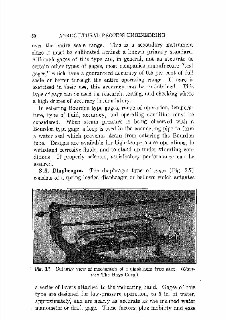
7/16/2019 Engenering Agriculture Perry
http://slidepdf.com/reader/full/engenering-agriculture-perry 59/422
50 AGRICULTURAL PROCESS ENGINEERING
over the entire scale range. This is a secondary instrument
since it must be calibrated against a known primary standard.Although gages of this type are, in general, not as accurate as
certain other types of gages, most companies manufacture "test
gages," which have a guaranteed accuracy of 0.5 per cent of full
scale or better through the entire operating range. I f care j,;
exercised in their use, this ac:cul'acy can he ma,intained. This
type of gage can be used for research, testing, and ehecking where
a high degree of accuracy is mandatory.
In selecting Bourdon type gages, range of operation, tempera
ture, type of fluid, accuracy, and operating condition must bc
considered. When cteam pressure is being observed with a
Bourdon type gage, a loop is used in the connecting pipe to form
a water seal which prevents steam from cntering the Bourdon
tube. Designs are available for high-ternperatme operations, to
withstand corrosive fluicls, and to stancl up under vibrating con
ditions. I f properly selected, satisfactory performance can be
assured.3.5. Diaphragm. The diaphragm type of gage (Fig. 3.7)
consists of a spring-loaded diaphragm or bellov,,'s which actuates
Fig. 3.7. Cutaway "iew of mechanism of a diaphragm type gage. (Courtesy The Hays Corp.)
a series of levers attached to the indicating hand. Gages of this
type are designed for low-pressure operation, to 5 in. of water,
approximately, and are nearly as accurate as the inclined water
manometer or draft gage. These factors, plus mobility and ease

7/16/2019 Engenering Agriculture Perry
http://slidepdf.com/reader/full/engenering-agriculture-perry 60/422
FLUID-FLOW MEASUREMENTS 51
of ollcration, place this gage in a superior position to the inclinedwater manometer for many jobs.
3.6. Gage Thl·ouling. Gages that are used for measurementswhere flow is fluctuating may vibrate or move otherwise, thereforeaccurate observations are impossible. Furthermore, the mechanical gages such as the Bourdon tube units may be damaged mechanically where excessive vibrations are encountered.
Gage installations on pumps, air anel refrigeration rompressol':',
and conduits where surging is experienced usually require proter'tion against fluctuation. This is provided by placing a restriction
in the gage line so the rate of flow through it is very slow. Adjustable valves, small orifires, 01' other restl'irtions that cut clown
the rate of flow but do not :-;hut it off ean be used. This procedure,
which is called throttling, gives It true [Lveragc of the varying
pressures at the point where the gage is attached.
VELOCITY MEASUREMENTS
3.7. Pitot Tube. The pitot tube is essentially an open tubepointing into the stream of fluid flowing as shown in Fig. 3.8. The
= = = = = = = = = = ~ ~ F P 8 = + P = V = = = =
Fig. 3.8. Elementary pitot tube.
impact of the moving fluid creates a pressure head nearly equalto V!!/2g, which is the velocity head of the Bernoulli equation.
The fluid static pressure or head which made up of the pressureand clcvntion heads is aclded to the pressure head so that a pres
sure gage attached to the tube indicates the sum of the velocity,
pressure, and elevation heads. A static pressure reading Ps istaken by the method descl'ibecl in a previous section; this readingis subtracted from the pitot total to give the net velocity or im
pact pressure. Pressure fittings are usually attached to a differ
ential gage, and the impact reading is made directly.
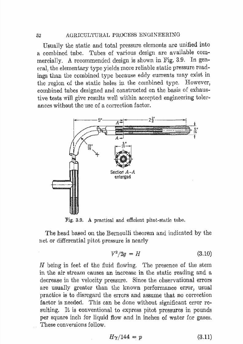
7/16/2019 Engenering Agriculture Perry
http://slidepdf.com/reader/full/engenering-agriculture-perry 61/422
52 AGRICULTURAL PROCESS ENGINEERING
Usually the static and total pressure elements are unified intoa combined tube. Tubes of various design are available com
mercially. A recommended design is shown in Fig. 3.9. In general
Jthe elementary type yields lllorc reliable static pressure read
ings than the combined type bccausc eddy currents may exist inthe region of the static holes in the combined type. However J
combined tubes designed and constructed on the basis of exhaustive tests will give results well within accepted engineering toler
ances without the use of a correction factor.
+ ~Section A-A
er.\arged
Fig. 3.9. A practical and efficient pitot-static tube.
The head based on the Bernoulli theorem and indicated by the
net or differential pitot pressure is nearly
V2/2g = H (3.10)
H being in feet of the fluid flowing. The presence of the stem
in the air stream causes an increase in the static reading and adecrease in the velocity pressure. Since the observational errorsare usually greater than the known performance error
lusual
practice is to disregard the errors and assume that no correction
factor is needed. This can be done without significant error reSUlting. It is conventional to express pitot pressures in poundsper square inch for liquid flow and in inches of water for gases.These conversions follow.
H-y/144 = p (3.11)
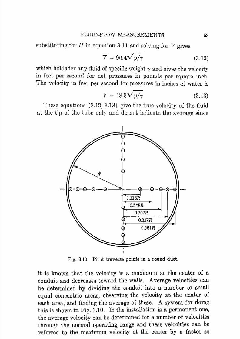
7/16/2019 Engenering Agriculture Perry
http://slidepdf.com/reader/full/engenering-agriculture-perry 62/422
FLUID-l?LOW MEASUREMENTS 53
substituting for H in eqllaLioIl 3.11 and solving for V gives
V = 96.4-v';h (3.12)which holds for any :fluid of specific weight 'Y and gives the velocityin feet per second for net pressures in pounds per square inch.The velocity in feei, per second for pressures in inches of water is
V = 18.3v'Ph (3.13)
These equations (3.12, 3.13) give the true vcloeity of the fluid
at the tip of the tube only find do not inrlieate the average since
CDI
CDIoI
CD
Io
I. -0-0-0-0--
i: :r .1-0 - 0 -
O.316R
, O.548R
O.707R
CD O.837R
Fig. 3.10. PiLot traverse points in a round duct.
it is known that the velocity is a maximum at the center of a
conduit and decreases toward the walls. Average velocities canbe determined by dividing the conduit into a number of small
equal concentric areas, observing the velocity at the center ofeach area, and finding the average of these. A system for doingthis is shown in Fig. 3.10. I f the installation is a permanent one,
the average velocity can be determined for a number of velocitiesthrough the normal operating range and these velocities can be
referred to the maximum velocity at the center by a factor so
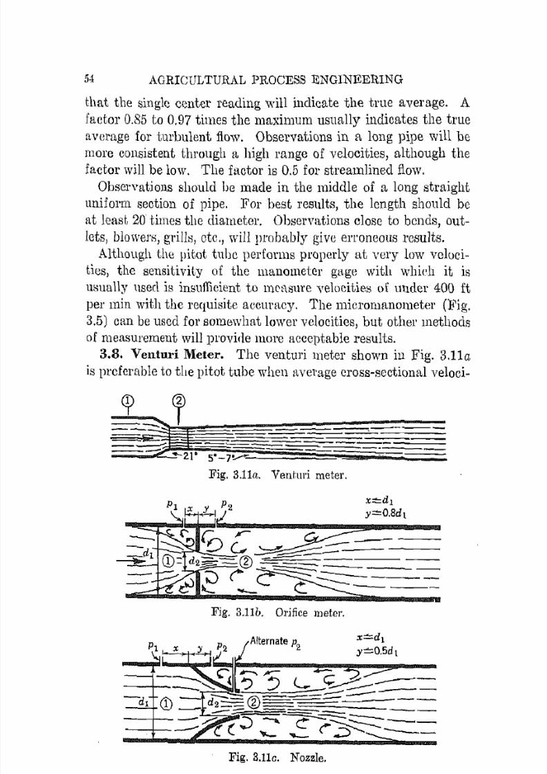
7/16/2019 Engenering Agriculture Perry
http://slidepdf.com/reader/full/engenering-agriculture-perry 63/422
54 AGRICULTURAL PROCESS ENGINEERING
that the single center reading will indicate the true average. A
factor 0.85 to 0.97 times the maximum usually indicates the true
average for turbulent flow. Observations in a long pipe will bemore consistent through a high range of velocities, although the
factor will be low. The factor is 0.5 for streamlined flow.
Observations should be made in the middle of a long straight
uniform section of pipe. For best reslllts, the length should bc
at least 20 times the diameter. Observations close to bends, out
lets, blowen5, grills, etc., willl1l'obably give erroneous results.
Although the pitot tube performs properly at very low veloci
ties, the sensitivity of the manometer gage with which it isusually llsecl is insuflieient to l l l l 'nSmC velocities of under 400 ft
per min with the requisite accuracy. The micl'omanoll1eter (Fig.
3.5) can be used for somewhat lower velocities, but other methodsof meaSllrement will provide more acceptable results.
3.8. Venturi Meter. The venturi meter shown in Fig. 3.lla
is preferable to tllC pitot tube when l1verage cross-sectional veloci-
Fig. 3.11a. Ventmi meter.
Fig. 3.lIb. Orifice meter.
Fig. 3.lle. Nozzle.
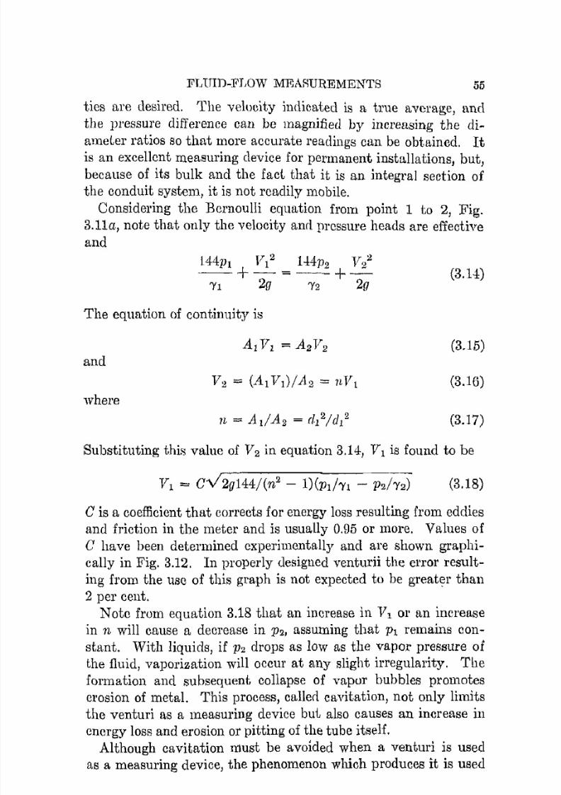
7/16/2019 Engenering Agriculture Perry
http://slidepdf.com/reader/full/engenering-agriculture-perry 64/422
FLUID-FLOW MEARUREMENTS 55
ties are desired. The veillcity indicated is a true average, and
the pressure difference can be magnified by increasing the di
ameLer ratios so that more accurate readings can be obtained. Itis an excellent measuring device for permanent installations, but,
because of its bulk and the fact that it is an integral section ofthe conduit system, it is not readily mobile.
Considering the Bernoulli equation from point 1 to 2, Fig.
3.11a, note that only the velocity amI pressure heads are effectiveand
(3.14)
The equation of continuity is
(3.15)and
(3.16)
where
(3.17)
Substituting this value of V2 in equation 3.14, V 1 is found to be
(3.18)
C is a coefficient that corrects for energy loss resulting from eddiesand friction in the meter and is usually 0.95 or more. Values of
C have been determined experimentally and are shown graphically in Fig. 3.12. In properly designed venturii the error result
ing from the use of this graph is not expected to be great!?r than
2 pel' cent.
Note from equation 3.18 that an increase in VI or an increasein n will cause a decrease in P2, assuming that Pl remains con
stant. With liquids, if P2 drops as low as the vapor pressure ofthe fluid, vaporization will occur at any slight irregularity. The
formation and subsequent collapse of vapor bubbles promotescrosion of metal. This process, callen cavitation, not only limitsthe venturi as a measuring device but also causes an increase in
cnergy loss and erosion or pitting of the tube itself.Although cavitation must be avoided when a venturi is used
as a measuring device, the phenomenon which produces it is used

7/16/2019 Engenering Agriculture Perry
http://slidepdf.com/reader/full/engenering-agriculture-perry 65/422
56 AGRICULTURAL PROCESS ENGINEERING
in certain types of pumps. I f VI and n are sufficient to produce
a P2 less than atmospheric, this rarefied pressure, vacuum, can
be used for evacuating or pumping. The laboratory suction pumpthat is fastened to a water faucet and basement sump pumps
operated off the house water systems are good examples of venturi
pumps.
1.00
0.98
0.96
C
0.94
0.92
0.90
0.883.0
VV ~
//
II3.4 3.8 4.2 4.6 5.0
L d 2v2 'YOg-".-
-
5.4 5.8 6.2 6.6
Pig. 3.12. Values of the venturi coefficient C referred to the log of Reyn
olds number.
The previous discussion applies to liquids where "/1 = "/2. I f
"/2!-'Il is nearly equal to 1, gases may be considered incompressibleand the error resulting is negligible. Ratios of 0.95 and 0.90 produce errors of 4 and 6 per cent respectively. Since it is advisable
to calibrate an individual tube against a known standard formost accurate results, preliminary calculations for gases can be
made with equation 3.18 without serious error resulting. Ven
tilation, drying, and air conditioning pressures with which theprocessing engineer is active seldom will exceed 4 in. of water.
The ratio for this pressure referred to atmospherjc at 14.7 psi is0.99, the resulting eITor being 0.5 per cent.
3.9. Orifices. Orifices and nozzles, Fig. 3.11b and 3.11c, areconvenient devices for measuring rates of flow because they are
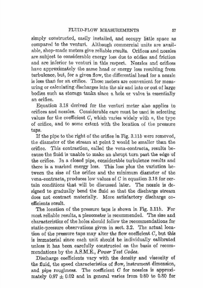
7/16/2019 Engenering Agriculture Perry
http://slidepdf.com/reader/full/engenering-agriculture-perry 66/422
FLUID-FLOW MEASUREMENTS 57
simply constructed, easily installed, and occupy little space ascompared to the venturi. Although commercial units are avail
able, shop-made meters givc reliable rcsults. Orifices and nozzlesare subject to eonsiderable energy loss due to eddies and frictionand are inferior to venturi in this respect. Nozzles and orifices
have approximately the same head or energy loss resulting from
turbulence, but, for a given flow, the differential head for a nozzleis less than for an orifice. These meters are convenient for meas
uring or calCUlating discharges into the air and into or out of largebodies such as storage tanks since a hole () l ' valve is essentially
an orifice.Equation 3.18 derived for the venturi meter also applies to
orifices and nozzles. Considerable care must be used in selecting
values for the coefficient C, which varies widely with n, the type
of orifice, and to some extent with the location of the pressure
taps.I f the pipe to the right of the orifice in Fig. 3.11b were removed,
the diameter of the stream at point 2 would be smaller than the
orifice. This contraction, called the vena-contracta, results because the fluid is unable to make an abrupt tum past the edge of
the orifice. In a closed pipe, considerable turbulence results andthere is a marked energy loss. This loss plus the variation bo
tween the size of the orifice and the minimum diameter of the
vena-contl'acta, produces low values of C in equation 3.1 8 for certain conditions that will be discussed later. The nozzle is designed to gradually bend the fluid so that the discharge stream
does not contract materially. More satisfactory discharge coefficients result.
The location of the pressure taps is shown in Fig. 3.11b. Formost reliable results, a piezometer is recommended. The size andcharacteristics of the holes should follow the recommendations for
static-pressure observations given in sect. 3.2. The actual location of the pressure taps may alter the flow coefficient C, but this
is immaterial since each unit should be individually calibrated
unless it has been carefully constructed on the basis of recommendations by the A.S.M.E., Power Test Codes.
Discharge coefficients vary with the density and viscosity of
the fluid, the speed characteristics of flow, instrument dimension,
and pipe roughness. The coefficient C for nozzles is approximately 0.97 ± 0.02 and in general varies from 0.60 to 0.80 for
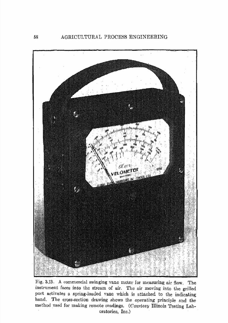
7/16/2019 Engenering Agriculture Perry
http://slidepdf.com/reader/full/engenering-agriculture-perry 67/422
58 AGRICULTURAL PROCESS ENGINEERING
Fig. 3.13. A commercial swinging vane meter for measuring air flow. Theinstrument faces into the stream of air. The ail' movjng into the grilled
port activates a spring-loaded vane which is attached to the indicatinghand. The cross-section drawing shows the operating principle and the
method useel for making remote readings. (Courtesy Illinois Testing Lab-
oratories, Inc.)
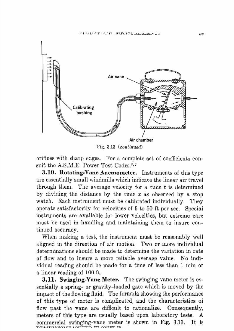
7/16/2019 Engenering Agriculture Perry
http://slidepdf.com/reader/full/engenering-agriculture-perry 68/422
FLUID-FLOW MEASUREMENTS
Calibratingbushing
Air chamber
Fig. 3.13 (continued)
59
orifices with sharp edget>. For a complete set of coefficients COll
suIt the A.S.M.E. Power Test C o d e s . ~ ' 7
3.10. Rotating-Vane Anemometer. Ini:itruments of this typeare essentially slllall windmills which indicate the lineal' air travel
through them. Thc average velocity for a time t is cletermined
by dividing the distance by the time x as o b ~ : ; e r v ( > d by a stop
watch. Each instrument must be calibrated individually. They
operate satisfactorily for velocities of 5 to 50 ft per sec. Special
instruments arc available for lower velocities, but extreme caremust be used in handling and maintaining them to insure con
tinued accuracy.When making a test, the instrument must be reasonably well
aligned in the direction of air motion. Two or more individual
determinations should be made to determine the variation in rate
of flow and to insure a more reliable U,VCl'age value. No individual reading should be made for a time of less than 1 min or
a linear reading of 100 ft.3.11. Swinging-Vane Meter. The swinging vane meter is es
sentially a spring- or gravity-loaded gate which is moved by theimpact of the Howing fluid. The formula showing the performance
of this type of meter is complicated, and the characteristics of
flow past the vane are difficult to rationalize. Consequently,meters of this type are usually based upon laboratory tests. A
commercial swinging-vane meter is shown in Fig. 3.13. I t is
7/16/2019 Engenering Agriculture Perry
http://slidepdf.com/reader/full/engenering-agriculture-perry 69/422
60 AGRICULTURAL PROCESS ENGINEERING
fitted and calibrated so that high and low air velocities and static
pressures can be observed both directly and remotely. Static
pressure observations are possible since a certain static pressureoperating through a definite resistancc will produce a definite
rate of flow through the instrument. The pressure-rate-of-flowrelationship is determined, and the instrument is also calibrated
in terms of pressure.The degree of accuracy of thc instrument depcnds upon the pre
cision of manufacture, calibration accuracy, and care in operation
and handling.
LOW·VELOCITY MEASUREMENTS
Low velocities, which for convenience are designated as lessthan 300 ft per min (5 ft per sec), may be difficult to measure,
particularly those of gases.Fortunately, the measurement of liquid velocities at low values
(lan usually be made easily and accurately. The devices dis
cussed under high velocity measurements operate satisfactorilysomewhat within the above-designated range because the specificweight is high enough to provide sufficient kinetic energy to
operate the gages used. Below this point, flow meters and gravimetric procedures may be used with suitable results because of
the relative incompressibility of the fiuid, high density (as compared with gases), and ease with which fluids can be confined.
Measurements of gas velocities below 300 ft per min are difficult
because the kinetic energy involved is insufficient to activate thegages used. Volumetric meters perform satisfactorily under certain conditions, but their use is limited. Natural convection c u r ~rents produce an additive en'or at low velocities which may completely confuse the results. In spite of the recognized difficulties,fairly reliable techniques have been developed for measuring gasvelocities, particularly air. A discussion of these techniquesfollows.
3.12. Katathermometer. The katathermometer is a largebulb alcohol thermometer of specific dimensions with 95° andlOO°F gradations only. The thermometer is heated in a waterbath or by other suitable means to a point above the 100° mark.
After the bllib is carefully dried, the thermometer is placed inthe air stream to be measured, and the time required for the bulb
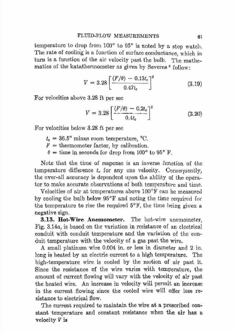
7/16/2019 Engenering Agriculture Perry
http://slidepdf.com/reader/full/engenering-agriculture-perry 70/422
FLUID-FLOW MEASUREMENTS 61
temperaturc to ch:op from 100° to 95° is noted by a stop watch.The rate of cooling is a fUlll'tion of surface conductance, which in
turn is a function of the air velocity past the bulb. The mathematics of the katathermometer as given by Severns 0 follow:
[(F Ie) - O.l3tcJ2
V = 3.28OA7to
For velocities above 3.28 it per sec
[
(FIe) - 0.2tcJ2
V = 3.28 OAte
For velocities below 3.28 ft per sec
te = 36.5° minus room temperature, °c.F = thermometer factor, by calibration.e = time in seconds for drop from 100° to 95° F.
(3.19)
(3.20)
Note that the time of response is an inverse function of the
temperature difference to for anyone velocity. Consequently,the over-all accuracy is dependent upon the ability of the opera
tor to make accurate observations of both tempcrature and time.Velocities of air at temperatures above 100°F can be measured
by cooling the bulb below 95°F and noting the time required for
the temperature to rise the required 5°F, the time being given a
negative sign.3.13. Hot-Wire Anemometer. The hot-wire l1nemometer,
Fig. 3.14a, is based on the variation in resistance of an electricalconduit with conduit temperature and the variation of the con
duit temperature with the velocity of a gas past the wire.A small platinum wire 0.004 in. or less in diameter and 2 in.
long is heated by an electric current to a high temperature. The
high-temperature wire is cooled by the motion of air past it.
Since the resistance of the wire varies with temperature, theamount of current flowing will vary with the velocity of air past
the heated wire. An increase in velocity will permit an increasein the current flowing since the cooled wire will offer less r e ~sistance to electrical flow.
The current required to maintain the wire at a prescribed c o n ~stant temperature and constant resistance when the air has a
velocity V is

7/16/2019 Engenering Agriculture Perry
http://slidepdf.com/reader/full/engenering-agriculture-perry 71/422
62 . ~ G R I C U L T U R A L PROCEtlS ENGINEERING
i Z = i02 + kVV (3.21)
where if) i!> the required current at zero velocity. Two methodsof mear·mrement arc used: the eonstant-resistance method and
the constant-current method.* In each method, the hot wire is
placed as one arm of a 'Vheatl'ltone bridge with suitable gages
and controls to adjust and observe operating conditions. The
hot-wire anemometer in FIg. 3.14a is wired to operate at con-
FIg. 3.14. HoL-wilC anemomerer, lea, and thermocouple anemomctcr, righL.
stant resistance. The resistances R1,
R 2,
and R3 of the Wheatstone bridge are adjusted so that the resistance of the hot wire
can be held at a e o n s t [ ~ n t prescrihed value by adjusting the
variable resistance R 4 • The velocity, then, is related to the cur
rent according to equation 3.21. The null reading io is taken by
covel·jng the hot wire with a small container which is assumed to
produce fltill air. Convection currcntfl set up by the heated wire
produce local air movement which makes the results question
able. I f the constant resistance-method is used, lc can be deter
mined for a single air velocity and the calibration curve can be
calculated. The instrument is caHbrated by attaching it to the
end of a long arm which is rotated in a room of still air. The
peripheral speed of the end of the arm at which point the meter
*Refer to Ower 6 for a detailed study of these methods.

7/16/2019 Engenering Agriculture Perry
http://slidepdf.com/reader/full/engenering-agriculture-perry 72/422
FLUID-FLOW MEASUREMENTS 63
is attached is considered the mte of air movement. This pro
cedure must be conrlucted with care else convection currents pro
duced by cold windows, walls, lights, radiators, motors, the operator, etc., will cause POOl' results, especially at low velocities.
3.14. Characteristics of Hot·Wire Anemometer. The hot
wire anemometer can he used for velocities as low as 6 i t pCI' min
by using i1 wire temperature in the artIer of 160°F. Wirc tem
pOl'atures are ilH'l'easecl for measuring higher velocities, 1800°],being used for velocities in the order of 800 ft per bee.
]'ree convection al'onnrl the heated wire introrluC'es tt constant
directional el'rnr which may amonnt to 30 ft per min for a 0.003-in.wire at 1800°F, and 15 ft per min at 400°F. Consequently, if low
v ( ~ l o c i t i e s arc to be measured, the instrument must be calibrated
under the same conditionR as those under which the tests will be
made or suitable cOl'l'ection procedures must be followed.
Heat energy is lost from the hot wire by radiationJ
but no cor
rection nced be made in this respect under normal conditions
because of the small area involved.
A significant errol' will result if the ambient air temperature is
significantly different from the ambient air temperature under
whi{'h calibration was carried out The lower the 'wire tempera
ture, the greater will be the error for a constant change in a m ~bient ail' temperature. Corrections can be made lor this varia
tion, but the procedure is too involved to be discussed here.
Although the hot-wire ancmometer can be used at low-wire
temperatures for measuring very low velocities, it perfol'lns best
under conditions of moderate to hot temperatures for measuring
moderate to high velocities.The direction of air motion must be known so that the hot wire
can be located perpendieular to it. II the wire is p l ~ e e d at an
angle to flow, low-velocity indications result. Corrections cannot
be made under this condition since the relationship between the
adjustment factor and angle is not known.
Fluctuating velocity is difficult to observe since the equipmentmust be balanced for each velocity. Automatic adjusting andrecording equipment can be used undcr fluctuating temperatures
i f the high cost can be justified.This measuring devicc can be used in a small space ancI operated
and observed from a remote location.
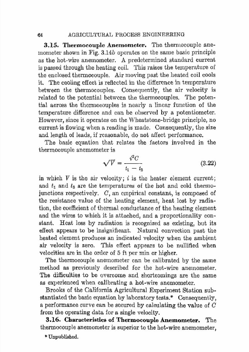
7/16/2019 Engenering Agriculture Perry
http://slidepdf.com/reader/full/engenering-agriculture-perry 73/422
64 AGRICULTURAL PROCESS ENGINEERING
3.15. Thermocouple Anemometer. The thermocouple ane
mometer shown in Fig. 3.14b operates on the same basic principle
as the hot-wire anemometer. A predetermined standard currentis passed through the beating coil. This raises the temperature ofthe enclosed thermocouple. Air moving past the heated coil cools
it. The cooling effect is reflected in the difference in temperaturebetween the thermocouples. Consequently, the air velocity is
related to the potential between the thermocouples. The potential across the thermocouples is nearly a linear function of the
temperature difference and can be observed by a potentiometer.
However, since it operates on the Wheatstone-bridge principle, nocurrent is flowing when a reading is made. Consequently, the sizeand length of leads, if reasonable, do not affect performance.
The basic equation that relates the factors involved in the
thermocouple anemometer is_ iZC
vV =-- (3.22)tl - tz
in which V is the air velocity i i is the heater element current;and t l and tz are the temperatures of the hot and cold thermo
junctions respectively. C, an empirical constant, is composed ofthe resistance value of the heating element, heat lost by radiation, the coefficient of thermal conductance of the heating element
and the wires to which it is attached, and a proportionality constant. Heat loss by radiation is recognized as existing, but its
effect appears to be insignificant. Natural convection past the
heated element produces an indicated velocity when the ambientair velocity is zero. This effect appears to be nullified when
velocities are in the order of 5 ft per min or higher.The thermocouple anemometer can be calibrated by the same
method as previously described for the hot-wire anemometer.The difficulties to be overcome and shortcomings are the same
as experienced when calibrating a hot-wire anemometer.
Brooks of the California Agricultural Experiment Station substantiated the basic equation by laboratory tests.* Consequently,
a performance curve can be sccured by calculating the value of Cfrom the operating data for a single velocity.
3.16. Characteristics of Thermocouple Anemometer. The
thermocouple anemometer is superior to the hot-wire anemometer,
'" UnpUblished.

7/16/2019 Engenering Agriculture Perry
http://slidepdf.com/reader/full/engenering-agriculture-perry 74/422
FLUID-FLOW MEASUREMENTS 65
especially for very low-velocity readings. The hot junction ismaintained initially at 15°-20°F above air temperature, whereas
the hot-wire anemometer must operate at 60 to 1700 degrees aboveail' temperature. Radiation and convection losses are small relative to the therlllocouple anemometer as compared to the hotwire anemometer, which operates at much higher temperatures.A normal change in air temperature docs not affect the performance of the thermocouple anemometer since the heating element is marle of Manganin, which has a constant resistancethrough a wide temperature range, and the two thermocouples are
referred to ambient air temperature.The thermocouple anemometer is affected by direction of ap
proach of the air. Fluctuations in velocity may create a readingdifficulty if an automatic recordcr is not used.
The thermocouple anemometer, like the hot-wire anemometer,can be placed in a small space and operated from a remotelocation.
3.17. Thomas Meter. This measming system is based upon
the rise in temperature that results from the introduction of heat. into a confined stream of flowing fluid that can be either llquid or
gaseous. An eloctrical heating element is placed in the stream of
flowing fluid and raises the temperature of the fluid.The relationship between the heat energy added, the tempera
ture elevation, and rate of flow is shown by the following formula.
0.0569 volt X ampv=-------
A 'C p (tl - t2)
(3.23)
where V ;= : fluid velocity, ft per min.A ;= : cross-sectional area, sq ft.I ' ;= : specific weight of fluid, Ib per cu ft.cp = specific heat of fluid, Btu per lb of at constant pressure.tl "" upstream or cool temperature, OF.
t2 = downstream or hot temperature, OF.
Temperatures are observed by resistance thermometers orthermocouples. They are connected to a milliammeter or potentiometer which indicates small temperature differentials ac
curately. The heating-element current is adjusted to maintaina constant temperature differential, usually of 2° to 5°F. Note
that the velocity is proportional to h e a t i n g ~ e l e m e n t amperage

7/16/2019 Engenering Agriculture Perry
http://slidepdf.com/reader/full/engenering-agriculture-perry 75/422
66 AGRICULTURAL PROCESS ENGINEERING
when a eonstant temperature differential is maintained. Small
temperature differentials arc advisable in order to minimize the
effect of heat loss by radiation anfl conduction throngh the walls.Losses by radiation can be eliminated by shielding the heating
element. Conduction losses ean he eliminated by insulating the
conduit containing the metering elements. Automatic recorders
can be set up by activating the heating-element rheostat through
the action of the galvanometer.3.18. Method of Mixtures. Rates of flow in confined conduits
can be det.ermined by mctcring a foreign fluid into the stream at
a definite I'atp, and sampling the mixture at a point downstreamwhere complete mixing is asslll'ed. I f an inert, gas is metered into
a stream of flowing air at atmospheric pressure, the percentage of
gas in the mixture as sampled indicates the rate of flow.
The percentage of gas in the mixture is
1'l'Om which
WgPg=----
Vky + Wg
V = : ~ (;g - 1)where V = rate of air flow, ft pel' min.
Wg = gas added, Ib per min.
A. = area of conduit, sq ft.
'Y = specific weight of ail', Ib pel' sq ft.
(3.24)
(3.25)
Pg=
percentage of gas in sampled mixture expressed as a
decimal.
In practice, the amount of gas added should be adjusted so that
the sample of gas mixture can be analyzed accurately. A com
parable procedme can be used for liquitls by introducing a stand
ardized salt solution into the flowing stream at a constant rate.
The concentration of the salt in the sample is determined by
titration or other suitable quantitative method.
3.19. Ammonium ChIOl·ide. The ammonium chloride generator shown in Fig. 3.15 can be used to observe and measure the
movement of air in a confined space such as a room, cold storage
locker, or storage house.
The motion of the dense doud of ammonium chloride which
is ejected into the atmosphere by operating the bulb will travel

7/16/2019 Engenering Agriculture Perry
http://slidepdf.com/reader/full/engenering-agriculture-perry 76/422
FLUlD-FLOVV MEASUREMENTS 67
with the air into which it is discharged. The lineal' speed anddirection can be observed.
The rate of settling of the particles is so fllow that they may beconsidered as moving perfectly with the air. Thi>J method is
'3uperior to that using smoke since there is no hent ('valved to
------ ----- -- - --
- - - ------------------ -
Fig. 3.15. Ammonium chloride generators.
produce convection. Best performance can be expected if thedevice is operated by remote control, by extending the aspirator
bulb tube. Thus, the body heat of the operator d o ~ s not affect
the rate of air movement.
FLOW MEASUREMENT
Flow implies a quantity, cubic feet, gallons, etc., flowing perunit of time as compared to velocity which implies lillear rates.

7/16/2019 Engenering Agriculture Perry
http://slidepdf.com/reader/full/engenering-agriculture-perry 77/422
68 AGRICULTURAL PROCESS ENGINEERING
The basic flow-measurement procedures are by weight and
volume per unit of time. Fluids flowing at a constant rate may
be run into or out of a container that is weighed at the beginningand end of a time period. The net 'weight increase divided by thetime provides the rate. There are comparable procedurcs which
use volume.Any of the velocity indicating or measuring devices discussed
in the previous section can be used to indicate flow by multiplyingthe cross-sectional area by the average velocity. For permanent
installations where the effective area is constant, gages and other
indicating devices are frequently calibrated to indicate rates offlow directly. Recording indicators are sometimes used to indi
cate the quantity accumulated or amount passed during a speci
fied time.Many other types of flow meters are available commercially.
They are complete units designed for specific installations and
conditions. The more common types are discussed in the following sections.
The following factors should be considered when selecting ameter for a specific job.
A, Operating conditions.
1. Characteristics of material to be metered.
2. Operating range.
3. Line pressure,
4. Characteristics of flow I steady or surging.
5. Required accuracy.B. Meter characteristics.
1. Operating range.
2, Accuracy through operating range and consistency ofcalibration with timc.
3. Resistance to corrosion.
4. Ability to be disassembled for cleaning i f used for foods.
GAS METERS
3.20. Bellows Meters. The familiar household gas meter, Fig.
3.16, consists of two bellows inner connected by valves. As one
bellows is being filled from the supply line} the other is emptying

7/16/2019 Engenering Agriculture Perry
http://slidepdf.com/reader/full/engenering-agriculture-perry 78/422
FLUID-FLOW MEASUREMENTS 69
into the service line. Valves f>hift the direction of flow at the end
of the stroke, and the emptied bellows fills from the supply line.The obcillation of the mechanism activates a volumetric indicator.
Flg. 316. Bellows gas meter. (Courtesy Pittsburgh Equitable Meter Division, Rockwell Manufacturing Co.)
The capacity varies from 75 to 10,000 cu ft per hr. Meters areavailable for operating pressures up to 1000 lb per sq in. Thepressure drop through the meter is usually in the order of 0.5 in.of water. The error of' a properly operating meter is lCilSS than1.0 per cent.
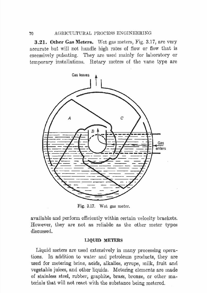
7/16/2019 Engenering Agriculture Perry
http://slidepdf.com/reader/full/engenering-agriculture-perry 79/422
70 AGRICULTURAL PROC.ESS ENGINEERING
3.21. Other Gas Meters. Wet gas meters, Fig. 3.17, are very
accurate but will not handle high rates of flow or flow that isexcessively pulsating. They are used mainly for laboratory or
temporary installations. Rotary motel'S of thc vane type are
Fig. 3.17. Wet gas meter.
available and perform efficiently within certain velocity brackets.
However, they are not as reliable as the other metcr types
discussed.
LIQUID METERS
Liquid meters are used extensively in many processing opera
tions. In addition to water and petroleum products, they areused for metering brine, acids, alkalies, symps, milk, fruit and
vegetable juices, and other liquids. Metering elements are made
of stainless steel, rubber, graphite, bras's, bronze, or other ma
terials that will not react with the substance being metered.

7/16/2019 Engenering Agriculture Perry
http://slidepdf.com/reader/full/engenering-agriculture-perry 80/422
FLUID-FLOW MEAt-i{TRgME::--.rTH 71
3.22. Piston Meters. Piston moter:;; are displacement or yolu
metric meters since thcy operate 011 the basis of and indicate the
volume, in cubic feet 01' gallons, of fluid paHsed in a rertain time.
The metcr is similar to Lhe hellows-type gas meter except thehellows are replaced by a double-acting piston. Two double
acting pistons at 900
connected to a crank shaft operate fo:tl1oother
than the single piston. The piston may be fitted with tight-fitterl
rings or with loosely fitted rings i f exact performance i:; notrequired. Although piston l l l e t e r ~ are availahle for water and
other liquids, their main usc is for commercial sale of petroleum
products where great accuracy is required.
,VeIl-designed piston meters operate with an error of less than
0.2 per cent through the entire operating range. Pressure (h'op iH
high becausc of tight-fitting pistons and may be 5 Ib per sq in.
at. a discharge rate of 100 gal per min, which is the approximate
maximum calmcity of a meter for use in a 2-in. line.
3.23. Disc and Cylinder Meters. Disc and cylinder meters
are recommended for most installations because they are reliable,reasonably accuratc, and economical. Disc and cylinder mcters
are displacement meters, although there is a small clearance be
tweon the moving element and the housing which pennits a small
amount of fluid to be by-passed. However, frictional clrag is low
and high degree of efficiency is attaineci. Two types are described.
A hard-rubber disc, frequently called a nutating- or wobble
disc meter is shown in Fig. 3.18. Thc slit in the disc engages the
pari.ition in the mctering chamber su that the disc is restrainedfrom rotating. The disc is supported on two hemispherical bear
ings whidl permit it to "wobble" but not to rotate. I t moves in
such a manner that a point on the circumferenco is continuously
in eontact with the top of the metering chamber, and an opposite
point, with the bottom of the mctering {'hamber, these points mov
ing around the chamber. The axis of thc disc moves ill such a
way that it generates a cone with the vertcx at the conter of the
disc. The partition directs fluid through a channel in the meterwhich is blocked by the disc. The disc lIlUst nutate or wobble to
permit the fluid to pass.Satisfactory performance can be expected for flows grea,ter than
1 gal pel' min. At lower rates the amount of fluid by-passing the

7/16/2019 Engenering Agriculture Perry
http://slidepdf.com/reader/full/engenering-agriculture-perry 81/422
72 AGRICULTURAL PROCESS ENGINEERING
disc is proportionally high. Rates up to 100 gal per min ms.y be
metered on a 1-in. line with an a,ccuracy of 98 per cent or better.
Noise and possible decreased efficiency due to wenr nfter pro
longed use are the objections to this type of meter. The pressure
drop through the meter is small.
Fig. 3.18. Nutating- or wobble-disc meter. (Courtesy Pittsburgh Equitable Motel' Division, Rockwell Manufacturing Co.)
The oscillating-piston meter shown and described in Fig. 3.19
is similar in principle to the disc meter but superior in performance because of less frictional drag nnd better balance. The
operating range is similar to that of the disc meter, but efficiencies
are higher and calibrahion is more reliable over a period of time.
Pressure drops are higher than for the disc meter. It is quiet inopel'ation.
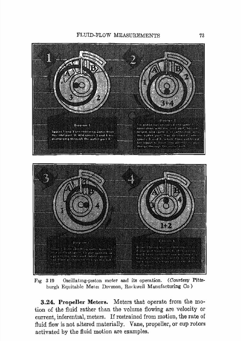
7/16/2019 Engenering Agriculture Perry
http://slidepdf.com/reader/full/engenering-agriculture-perry 82/422
FLUID-FLoW MEASUREMENTS 73
FIg 3 19 O ~ c i I 1 a t m g - p l s t o n meter and its operation. (Courtesy Pitts-burgh Equitable Me1el DIvIsion, Rorkwell Manufacturing Co)
3.24. Propeller Meters. Meters that operate from the mo
tion of the fluid rathel' than the volume flowing are velocity orcurrent, inferentIal, meters. I f restrained from motion, the rate of
fluid flow is not altered materially, Vane, propeller, or cup rotors
activated by the fluid motion are examples.

7/16/2019 Engenering Agriculture Perry
http://slidepdf.com/reader/full/engenering-agriculture-perry 83/422
N AGRIcULTURAL PROCESS ENGINEERING
They nre IllO:-;t u::;cful for continuous high rates of flow such as
might he found in washing, irrigation, or general supply lines.
They are not efficient at low rates of flow because of bearing
friction. I<'luids containing solid matter such as flirt and sand
can he metered satisfactorily.
A pl"o]1eller meter is SIHrWIl in Fig. 3.20.
Fig. 3.20. A propeller mctur. (Courtesy Pitt.sburgh Equitable Meter Division, Roekwell Manufacturing Co.)
3.25. RotameLel's. A commercial rotameter and its schematic
elements arc shuwn in Fig. 3.21. The rotor is supported by the
upward motion of the fluid, and its position in the tube indicates
the rate of flow.
The rotor is stationary when tIlt' upward force resulting from
flow equals the rotor's weight, or
G7rd2",/ V2
=W (3.2G)8g(144)
or
V = 153VW/d2",/C (3.27)

7/16/2019 Engenering Agriculture Perry
http://slidepdf.com/reader/full/engenering-agriculture-perry 84/422
F'LfTID-FLOW lVU;AHURKlvrENTS
where V = velocity of fluid aL Hmalle::;t eI'OH::> Heetion, ft pel' Hee.
d = mlLximUffi rotor diameter, in.
'Y = Rpecifie \wight of ftuicl.
75
C = rotor drag eodfieient; varieH with rotor shapr and
fluid flo wing.
TV = weight of rotor, lb.
~ i n l ' e the velocity in the above' equatioll nUlHt remain c'ollHtant,
the fuUowinp; re\atl0m'lhip hohb.
( : ~ . 2 ~ )
in which Q iH H q\lantity \'alp and the ('(Ill:'! ant k ii'i lIludp up of
7T/4 and the rcquired ('onstanj Yeloeily value.
D=D 1+mLH
L
Dl
Fig. 3.21. A commercial rotameter with important details shown. (Cour
tesy Schutte and Koerting Co.)
7/16/2019 Engenering Agriculture Perry
http://slidepdf.com/reader/full/engenering-agriculture-perry 85/422
76 AGRICULTURAL PROCESS ENGINEERING
Now, if the difference between ])2 and d2 is small as compared
Lo d2, Q may be considered as a linear funcLion of m (D - d)
without introducing an error greater than permitted in most engineering work. I f a high degree of accuracy is required, the
meter can be calibrated through its entire range against, a known
si;andard.
Rotameters can be used for liquids 01' gases. Chemicals, oils,
food products, and fluids cHl'l'ying suspended solid material can
be metered. Large 01' small quantity rates can be handled. The
pressure drop through the meter is nominal.
REFERENCES
1. Addison, H. Hyrl),(1Il1ic MC(ls1tl'em(mts. Second Edition. Wiley. 1946.
2. Fluid Meters, Their 'Theory and Applicat.ions. Report of A.R.M.E. Spe
cial Research Committee on Fluid Meiers, Part 1. A.S.M.E. 1937.
3. Folsom, R. G., amI Iverson, H. W. Pipe Factors for Quantity Rate
Flow Measurements with Pitot Tubes. A..S.M.E. Paper 48-A-35.1948.
4. Amer. Inst. of Physics. Tempemtul'e, It s M eaSU1'ement and Control inScience and Industry,. Papers presented at a symrJosium, Pp. 666-672.Rheinhold. 1941.
.5. Merriam, K. C., and Spaulding, E. R. Comparative Tests of Pitot
Static Tubes. National A d v i . ~ m · y Committee for Aeronautics. Tech.
Note 546. November, 1935.
6. Ower, E. 'l'he Measnrerncnt of Air Flow. Chapman & RaIl. 1933.
7. Power Test Codos. Information on InBlrmnonts and ApPQmtus, PnJ't .5,
Measurement of QUantity of Material5; Chapter 4, Flow Measure
ment by Means of Standardized Nozzles and Orifice Plates. A.S.M.E.
1940.
8. Seban, R. A., et a!. A Thermal Anemometer for Low Velocity Flow.
'['rans. A.S.iVI.E. 65:843-846. 1943.
9. Severns, W. H. Healing, Ventilating [lnd Ail' Conditioning J.illndamen
t a l , ~ . Second Edition. Wiley. 1949.
10. Smith, H. W. Improved Micl'omllnometcr. Ind. Eng. Cham" A.nal.Ed. 8: 151-1.52. March, 1936.
PROBLEMS
1. A water pressure gauge located 4 ft above a pressure SOUl'CO reads 21 Ib
per sq in. The connecting tube is full of liquid. What is the actual
pressure at the source?
2. The system of problem 1 is initially full of air at atmospheric pressure.
The main line was then filled with water, no air being bled from the
7/16/2019 Engenering Agriculture Perry
http://slidepdf.com/reader/full/engenering-agriculture-perry 86/422
FLUID-leLOW MEAi:lUREMENTS 77
gage connecting, pipe. What, is the pn'ob1ll'C in the maiu liue if the gageagain indieates 21 Ib pel' sq in.?
3. Ail' at 70" is being measured by a nutll l ' i metcr with basic diametersof 14 and 10 in., respectively. Gages aUached at puints 1 und 2, Fig.3.l1a, read 5.75 and 2.10 in. of water. What quantity of air is flowing?
4. The gage on [tIl orince meter reads 41;2 Ih prr Sf[ in. What is thE' velocityof water if the inside pipe diameter is 1.25 in. and sharp-erlgedorifice is 0.89 in. in diametel'? (C =: 0.76.)
5. A nozzle metel' is to be designed to fit into an IS-in. galv(mizrd pipe.Air at room tempemlurc flows through Lhe pipe at velocities varying
from 700 to 1400 fL per min. I f [ i 2-in. ineJillP.d manometer eontainillg
alcohol with a S.G. of 0.89 is to be used with the ncJzzl0, what should
be the diameter of the nozzlo !6. A Thomas IDP1er is located in an ail' duct of 2 Si l ft moss-sectional area.
The air weighs 0.083 Ib per Cll ft, and its specific heat is 0.24. Assume
a controlled tempcratme differentiul of 5° an(i Iwater potential of 110
volts. Plot the velocity as abscissJ1 and amperage as ordinate for velocity 0 to 300 ft per min. Assume constant amperage of 3, and plot tem
perature difference against velocity. Discuss the l 'UlTCS from the stand
point of accuracy of the system.
7. A differenUal piLot tube locat.ed at the center of a cylindrical air tubeproduces 2.6 in. of water pressure. What is the velocity at the impact
eud uf the pitot tube? The impact gauge read>! 2.6, 2.6, 2.5, 2.1, 1.8
when placed at points 1-5 in Fig. 3.10. WlHl.t is the ilVel'llge velocity inthe tube? What factor would bQ applied to the center reading to indi
cate a true [1verage velocity'! Nute: In ademl practice it would be
necessary to check this factor through the entire J'ltllgC of velocities to
be encountered, because variation Illay he expedeu.
8. A pump is moving soybean oil through a I-in. (nominal) pipe. The
110-volt motor is using 285 waLts. A ~ s u m i n g Ull oyer-all pump and
motor efficiency of 65 per cent, what is the pumping rate in gallons pE'l'
minute i f the suction and discharge] l r C S ~ \ l l ' e R
are, respectively, -5 and23 lb per sq in.?9. CarLon dioxide is metered intll an nil' cOllrlllit. which is 12 sq ft in
cross-sectional area at a constant rate of 7.0 Ih jJer hour. A sample of
the mixture downstream waR analyzed by au OrsaL IlPPuratus and con
tained 11% per cent CO 2 by volume. What is the air velocit.y?
7/16/2019 Engenering Agriculture Perry
http://slidepdf.com/reader/full/engenering-agriculture-perry 87/422
C H A PT E R 4
NOMENCLATURE
i l = nross-snctioIl111 lLrea, sq fL.
C = a pTOportionalit.y GOJlsLant.
D = diameter, in.
l { = total hoarl, ft of fluid flowing.
lis = pressure, C I C v ~ L t i o I l , mid friction head, ft of fluid flowing.
h, = lift, ft .h., = submergence, ft.
hp = horsepower.
N = revolutions pOl' minute.
Q == a qUlLntity of air, en rt per glLI water.
1/ = eu ft por sec.l ! = fluid veloclity rclative to housing, ft per S('G.
VI = fluid velocity relative to housing tangent to runner, ft per sec.
V,. = fluid veloeity relative to VlillG, ft per ~ e e .v = peripheral speed of runner, ft per sec.
w = vane width, ft .
V = mdial fiuid vcloeity, ft pel' sec.I ' = specific weight, III per eu ft.
Pumps are generally considered as devices for elevating or
moving liquids. Although this is a satisfactory conception incertain regards, it would be more exact to state that they increase
the work head tV in the Bernoulli equation (2.71. This restate
ment implies that the pumping effect upon the fluid might be to
elevate the fluid, change its internal pressun', or change its
velocity, 01' a combination of any of these.
The processing engineer is interm;ted in the performance of
these devices from the standpoint of their effect upon the three
factors indicated above, elevation head, pressure head, and velocity head, and their interrelation when one or more are changed.
His chief job will be selection and installation rather than design.
For convenience in discussion, these devices will be classed as
follows:78

7/16/2019 Engenering Agriculture Perry
http://slidepdf.com/reader/full/engenering-agriculture-perry 88/422
PUMP:-;
Pm;itinl clil:)lllacement pump,,: l'ceiproeutillg and rotary
.Tet pumps.
Air lifts.
Centrifugal p u m ( l ~ .
7!J
4,.1. Evaluating Performance. The Illl'('hHlli('all'fneiel1CY of
thesp rleviee:; is the ratio of Ow wurk output to the input" Ute' O\lt
put being the pro(hwt of the elwnge in tll(' toialenl·\'i.\Y hC'ad IT
times the \Vl'ight of £lui(l il()wing pel' minute an(l the input l 'X
presRecl HI'; f o o t - l l ( ) u n d ~ prr minute. If the input ii' ( , x l n ' ( ' s ~ l ' d itt
horsepower, the equation iR,
!J X Ll) fluid flowing pE'l' minHydmulie effieiency =
hp >< 33,000
Volumetric effieiency that ttppliel:) to p o ~ i t i y c di:>plaeemeni,
pump8 only iR the ratio of the volume of fiui(l moved pcr ulliL of
time to the pislon di:;plaeemcnt per unit of time.
PUNIP TYPES
The re('iprocating or 11isLon type of pump has been healed in
previous eoun.,es anrl is well cnough known so that a dotailt'cl c l i ~ cussion will be omitted. The meclumical effi('ienry of thcse pumptl
may be fit> high as 80 to 90 per ecnt, the lOSH hping dne in the main
to frietion. Fluids containing ttbrasive materials or ( ' o r r o ~ i y efluids cannut be pmnpe(l with ordinary recilll'0('atil1!S pumps.
They arc specially well ac1apted for h i g h - p r e ~ s u r e operation.
4.2. Rotary Pumps. The rotary pUnlptl, Figs. 4.1, 4.2, aTIlI
4.:3, are positive displacemcnt units and are inCXpClltiive un(1
simple to construct. I f constructed [tllli maintained with very
close tolerallC'Ctl, the volumetric l·fficicney ii:l high ttlHl high 1)1'('8-
Rure:; CUll be produced. A slllall unit can handk largo quantities
of fiuirl heeause high rotHtive speed,; nrc l l O : ; ~ i b l ( ' . 1\1ecllan1C'[ll
effieiencie8 may be 90 }leI' cent or more uncler the best condition:;.
Gen.r pumps are well suited for muny proeoi:;:,ing oj)emti(]llf:.
since they arc positive acting, provide a continuous :,;mooth flow
of material, do not whip the mntcrial when pnll1J1o,l, and a1'('
ear:;ily disas8cmblcd for cleaning. They ::11'e speciaHy suitable for
viscous substances such as ice-cream mix, molasseR, and oils.

7/16/2019 Engenering Agriculture Perry
http://slidepdf.com/reader/full/engenering-agriculture-perry 89/422
80 AGRICULTURAL PROCESS ENGINEERING
Gear pumps perforlll best when pumping fluids with some lubricating properties. However, external gears arc frequently pro-
Fig. 4.1. Internal-gear rotary pump.
Fig. 4.2. E x t e r n a l ~ g e a r rotary pump.
vided to maintain pumping-gear alignment. This feature permitsnonlubricating fluids to be pumped with a minimum of wear to
the pump. For high-pressure operation, close tolerances must be

7/16/2019 Engenering Agriculture Perry
http://slidepdf.com/reader/full/engenering-agriculture-perry 90/422
PUMPS 81
piovided and mamt,lIned SatI'5fJ.cboI YPCI fOlll1.11lLe p e h l ~ t s only
If clo::,c tolmanLes ale mamtamed
Flg 4 d Lobe pump, used for both g,lseb uud hql1lds
Vane pumpb are chawctenzcd by bhclmg VltnCS ::,uch a1> shown
in FIg, 44, cylmclncal seals 1Il slot<" awl Innged lobe<, or other
detaIls fOl mamtall11l1g a seJ.llll the pump Tlus pump, ,tlthouglt
:FIg 44 Vane pump, used for both gases and hqUlr[s.
more ::,ubJect to wear than othel lOtary pumps, can develop a l11gh
pressure because of a better seal between the rotor and the hous
ing. Its chief use m the procesbmg field is evacuating, partwu-

7/16/2019 Engenering Agriculture Perry
http://slidepdf.com/reader/full/engenering-agriculture-perry 91/422
82 AGRICULTlTRAL PROCESS ENGINEERING
lal'ly for dry VnCllUll1 pump work sucl! [IS that done by milking
machines and vacuum pans.
4.3. Jet Pumps. The jet pump shown elementarily in Fig.'!.[i operates on the velocity energy of a jet of fluid. Water (or
L=====..:-___::>,..., \
Optional
Centrifugal
pump
, \\ \
\ II II II II II II II I
I I
Fig. 4.1i, S l ' , h r ~ m : l t i < : d p m p l l t . ~ of I l jet. pump.
other fluid, either compressible or incomprestlible) is forcedthrough a jet or nozzle of such dimensiuns that all ur nearly all
the energy involved is converted into velocity energy. This
energy, which is directional, is applied to the fluid to be moved.
The jet is produced by recirculating a portion of the liquid or
gas in those cases where the material will not damage the pump.
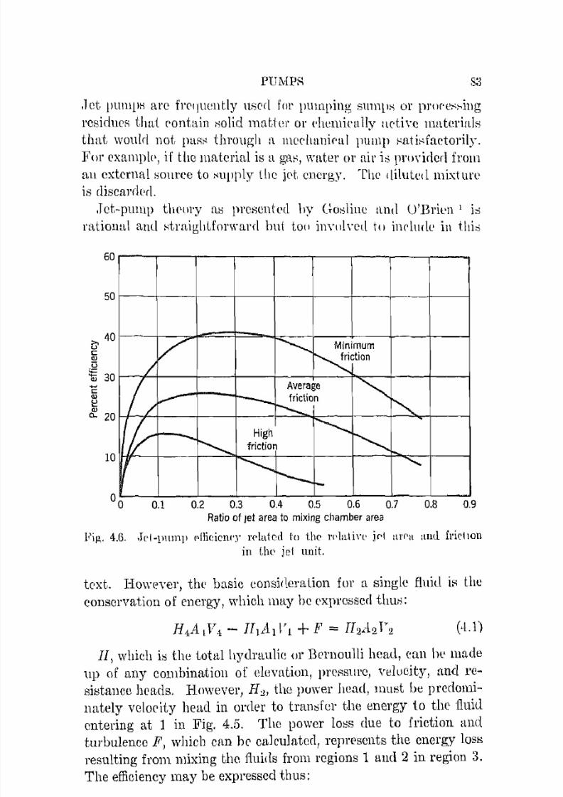
7/16/2019 Engenering Agriculture Perry
http://slidepdf.com/reader/full/engenering-agriculture-perry 92/422
PUMPR S·,, )
,1 et pump" arc fr('IjUclltly 118('(1 for pUlllPing; Slimp" or P]'(I['C:-::--illg
residues thai. ('ontain Holie! mattul' or l'lwmieally lletiyc materials
that would not, p a R ~ through n llleeltani('ltl j1\;IllP r:atiHfuctol'ily.For examph', if the material is n gal', water or nil' is p1'Oyirlerl from
an external H01ll'ee to Hupply the kt energy. The diluted mixtut'l'is disca]'(JL.r1.
.let-pump thelll'Y [1:-; pre8cnted hy Oo:-;lillc and U'Bril'll I is
ratiollal and ~ t r a i g l l L f o r w a r r l but top inYIllyed til indude ill this
60
50
>. 40u
53u~ 30- ,!:!Q)
0.. 20
10
v- I'---- Minimum
/~ c t i o n
//
Average ~r - - friction
'"-....( ~ I .-- . High ~ ~..... .........._ friction
II ............... ""r--I -
0.1 0.2 0.3 0.4 0.5 0.6 0.7 0.8 0.9Ratio of Jet area to mixing chamber area
Fip,. 4.6. ,Jpi-lllllnp f'nieiCll('J' rp\atcd to tho rl'\alin' jC'l ar('a aIlll fricllOn
in lIw iet unit.
text. Howeyer, the basic consirleralion fur a single fluid io; the
conscrvation of energy, which may bc ('xpresserl tllUll:
(-l.U
11, which i:-; the total hydraulic: or Bernoulli head, can \w made
up of nny combination of elevation, i)J'l'RSUl'C, yelucity, and 1'0-
si.stance heads. However, H2 , the puwer head, must be predomi
nately velority head in order to trant;fcr the energy 1.0 the fluid
entering at 1 in Fig. 4.5. The power 10::;8 due to friction and
turbulence F, which cnn br calculated, represents the energy loss
resulting from mixing the fluids from regions 1 and 2 in region 3.
The efficiency may be expressed thus:

7/16/2019 Engenering Agriculture Perry
http://slidepdf.com/reader/full/engenering-agriculture-perry 93/422
84 AGRICULTURAL PROCESS ENGINEERING
H4A4 V'l - HIA l 111
H2A2T'2
(4.2)
The efficiency is closely related to the ratio of the nozzle area
to the mixing-cylinder area and the friction in thc system. The
relationships of these factors as reported by Gosline and O'Brien
are shown in Fig. 4.6. These are theoretical curves that have
been substantiated by observation.
In spite of its low efficiency, the simplicity of the jet purnp, itsfreedom from moving parts, its ability to pump materials of
sludge consistency, and its low initial cost fit it for use in situations where other pumping devices would be impractical.
4,.4. Air Lift. Another convenient device for elevating liquids
is the air lift shown in Fig. 4.7. Air is delivered at the bottom of
the lift pipe and mixes with the liquid. The air-liquid mixture,
Air in underpressure
Fig. 4.7. The air lift.

7/16/2019 Engenering Agriculture Perry
http://slidepdf.com/reader/full/engenering-agriculture-perry 94/422
rUMPS 85
being of less specific weighi, than the liquid, rises in the pipe and
is dischargl'd at a point above the level of the liquid.
An empirieal formula hiLs Leen developed by the Ingersoll-RandCompany for design where water is the fluid being lifted. I t is
Q = 0.8 hiC log [(h. + 34)/34]
where Q = eu f t free air recluil'ed to lift 1 gal of water.hi = lift, ft.
(4.3)
hs = submergence, clistanee from surface of water to point
of air introduction, ft.C = a constant (note table).
Lift hI! jt C
10-00 24561-200 233
201-500 216501-650 l85651-750 156
The submergence, expressed as the ratio ht/ (h a+ h,), should
vary from 0.66 for a lift of 20 ft to 0.41 for a lift of 500 ft. Foot
picce design is important ::linee the size and distriLution of air
bubblcs maLcl'ially affect the efficicncy. The ail' compressor must
be able to ::lupply air at a pressure head equal to hs and in a quan
tity specified by equation 4.3.
This lifting device * can be employed for fiukls containing for
eign materials nnd for corrosive liquids. From 20 to 40 pel' cent
of the energy uHed to C0111pre1:lS the air is l'iIcctive in elevn,ting the
liquid.
4,.5. Ceutrifugal Pump. The centrifugal pump is widely used
for pumping watcr, milk, lubricnnts, chemical solutions, materials
being processed, etc. Its popularity is due to rclative simplicity,
mechanical effieiencies as high as 90 per cent under favorable
conditions, and ability to handle fluids containing solids in sus
pcnsion. Centrifugal pumps can be designed for high-pressureoperaLion where necessary. Because of simplicity and ease of
disassembling, which facilitate cleaning, washing, and sterilizing,
they are satisfactory for food pl'oducts.
*This device is nol, a pump in the stl'il,test sense since it cannot alter thepressure or velocity heads in the Bernoulli equation in any practical degree.

7/16/2019 Engenering Agriculture Perry
http://slidepdf.com/reader/full/engenering-agriculture-perry 95/422
86 AGIUCfTLTURAL PROCESS ENGINEERING
The hasic principles of design that also apply to fans and
blowers are important to an understanding of performance and
Jll'oper selection. Considering Fig. 4.8 we assume that (1) theblade thickneCis is negligible; (2) friction losses are negligible;
ane[ (3) the peripheral velocity at the inlet is zero.
- - - - - -.....-...--
//1'"",,,,
//
I
I /
IIIIIIII\\\\\\
\\.
'-' ....,
.... , ..... _ . -
------Fig. 4.8. V ~ l o e i t . y veet.ors for II ef'nt.rifugal-pUlnp runner.
The angular momentum of the water immediately after lenving
the impeller is
which may also be considered the torque exerted on and by the
impeller. The work clone pel' second by the impeller upon the
water is
Torque X Angular velocity = (W/g)l'n' X v/r = (W/g)V1v (4.5)
The work input per second (01' other unit of time) per pound ofwater flowing is
(V1v)/g

7/16/2019 Engenering Agriculture Perry
http://slidepdf.com/reader/full/engenering-agriculture-perry 96/422
PUl\Il'R 87
I f thE' input is l'eft'l'l'Pcl 1,0 a 1'e[p1'once plane through thl' pump,
the output from tIl(' ::.tanrlpoint of Bl'l'I1oulli's tll£'urem is
(4.7)
in which H 8 may be e i t h ( ~ 1 ' Pl'PH::m1'C, friction, or elp\-atiul) head or
a combination of them. Erluating equations -Ui and -1. 7, tIl(' thc
Ill'etical mechanical-energy balance is
or
Now r 2= vi + ':2 and Yr = v - .II eot a, from which
= (v - .If ('ot a? + l
Substituting for y2 and Y r in equation -f.9 gives
( )9"
H = 2v v - y cot a - (v - y cot a)- + y ~
2gwhieh when solved becomes
20or
.-) 0) i )
v- y- ese- a-=Hs+---2g 2g
(-l.9)
(·1.10)
(oUl)
( .U2)
U·13)
Consider the meHning of this equation from the l':ltancl_point ofpump design and selection. The first term v!l/2fj is directly re
lated to the sIleed of the runner. lIs is i.he static friction and/or
elevation heac! a g a i l l ~ t which the pump i::; operated. The mte of
dit':dmrge equals 27rl'1uy and is represcnted by y. The shape and
depth of the vane are the two basic clc:t;ign features t11at affectperforman('e. Assuming no friction loss in the runner and a con
stant speed, that is, v constant, note the folluwing very ~ i g n i f i e a n tfeatures.
1. I f the operating head I i is increased, the rate of discharg,e
represented here by y, decreases. This response is a charaderistie
feature of centrifugal pumps.
2. The discharge velocity y may be varied by the runnel' de
sign. Since the mass rate must oe the same at the inner amI outer
7/16/2019 Engenering Agriculture Perry
http://slidepdf.com/reader/full/engenering-agriculture-perry 97/422
88 AGRICULTURAL PROCESS ENGINEERING
peripheries, the capacity per revolution = 27r1"wy = 27rr'w'y', inwhich the prime values are at the inner periphery. The velocity
y decreases as r' decreases and as w' decreases. y is not constant, because of resistance loads. Therefore, pumps with deepvanes and narrow inner peripheries produce high static heads with
low discharge rates.3. An increase in the vane pitch angle permits a decrease in the
revolutions pel' minute required for a certain discharge and de
creases the maximum head uncleI' which satisfactory performancecan be expected.
4. The total theoretical head at complete shut-off is equal to thesquare of the peripheral speed divided by 2g, equation 4.12 with y
equal to O. Actual shut-off heads sometimes exceed the theoreti
cal. This occurrence is believed to be due to fluid circulationwithin the pump casing.
Pumps are used to move a quantity of fluid against a resistance which may be attributable to elevation 01' friction of
conduits, nozzles, and other fittings. Therefore, the velocity head .
produced by a pump should be converted to static head H. Thisconversion is attempted by graclual reduction of the velocity inone of two ways.
Diffuser or guide vanes may conduct the fluid away from theimpeller and gradually lower its vclocity by increasing the con
duit area. The reduction in velocity effects an increase in pressure head as a result of the operation of the Bernoulli equation.
The vanes are so bent that the water is turned gradually and is
finally discharged into a manifold.A second method, which is simpler and less expensive, is the
volute manifold or casing outlined by the dotted line in Fig. 4.8.
The casing is so designed that the u.verage velocity is constant
at all cross sections and is approximately V 2 in Fig. 4.8. Whenproperly designed, each fluid element is gradually turned toward
the discharge outlet so that turbulence losses are at a minimum.
Further reduction in velocity effect may be had by gradually
expanding the diameter of the discharge pipe.4.6. Performance, Testing, and Rating. The American So
ciety of Mechanical Engineers and the Hydraulic Institute 5,7
have developed standard methods for testing centrifugal androtary pumps. These test code series should be studied if formal

7/16/2019 Engenering Agriculture Perry
http://slidepdf.com/reader/full/engenering-agriculture-perry 98/422
PUMPS 81l
tests are to he made or perfOrnl[lllre data bubjccied to a critical
analysis.
Tesis arc m[l(lc by operating the pump at a {'Ol1stant speed and
varying the capacity by throWing the Qntle't. Thc total head,
the yelocity head, and perhaps the static head arc platte! 1 against
the ratc of c1iflcharge. The horsepower input und efficiency arealso determined and plotted against the Ilischargc rate. The
5 0 r - ~ ~ ~ ~ = = r - - - ~ - - ~ - - ~ - - ~ - - '
~ 3 0 r - - - - r - - ~ ~ - - ~ - - ~ - - - - ~ - - ~ ~ ~ ·-0al
x 2 0 ~ - ; t - - - ~ ~ ~ - - - i - - - - r - ~ ~ ~ ~ ~ ~
25 50 75 100 125 150 175Capacity, gallons per mmute
4
3
:;;;;:
2g.~::c
- 80
60 ".,uc
'"40 :m~
cOJ
OJ
20 fl .
o
Fig. 4.9. A l ' e p l ' e ~ e n t a t i v e standat'd centrifugal-pump test plot.
horsepower input to thc pump I',haft is determined by any of
the aecepted procedures. Calibrated electric motors are included.
The efficiency is expressed as t.he ratio of thc fluid horsepower to
the shaft horsepower where,
Fluid horsepower = q,,{fI/550
where q = Cll ft fluid per sec.
'Y ::::: fluid specific weight, Ib per cu ft.
H = total head, ft.
(4.14)
A complete performance study would include a series of tests
made at different pump speeds.
A representative pump test plot is shown in Fig. 4.9. The
pump is a 2 X 2* X 7" pump direct connected to an electric
motor that operates at 1700 rpm. Note that some power is re
quired at the no-discharge position.
*Outlet 2 in. in diameter, inlet in., and runner 7 in. in diameter.

7/16/2019 Engenering Agriculture Perry
http://slidepdf.com/reader/full/engenering-agriculture-perry 99/422
90 AGRICULTURAL PROCESS ENGINEERING
A HpeciflC job would require a pump with a spe(!ifiecl capacity
at f\ specified heac!. Selection would be made from H series of
test plots for different-size pumps. As a general rule it is ["Lel
visable to select a pump so constructed that the point of per
forrnanee will f[dl to the right of the maximum efficiency point
on the test. :sheet. Thcn, if the opcrating head increases after
being plll.ced in operation, the effiriency will not be affected and
60
0 0 20 40 60 80 100 120 140 160 180 200 220 240 260
Gallons per minute
Fig. 4.10. p ( ~ l ' f O l ' l l l l l n e C (httn for ll. 2 X 2 X 8 in., 1760 rpm ('entrifugal
pump with impellers ranging in diameter (D) from 5 Lo 8 in.
the capacitywill
not be lowered significantly. For example, if
the total head is increased from 35 to "10 ft because of adtled lift
or restriction in the line, the c:apaeity will drop from 145 to 125
gal per min, 14 per cent, and the effieicncy will incl'ease from 74
to 78 per cont. On thc other hand, a similar total head increase
from 42112 to 47% ft would reduce the capacity from 112]12 to
80 ft, a reduction of 2H per cent as cornpal'ecl to 14 per cent above.
The efficiency would decrease from 79 to 74 pel' cent.
Performance data are sometimes presented as shown in Fig.
4.10. This isoefficieney plot shows the performance of a pump
with a number of differel1t runners. Similar plots with a single
runner operating at different speeds are common. Selection
should usually be made to tho right and below the point of high
est efficienuy for reasons as noted above.
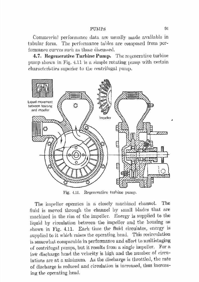
7/16/2019 Engenering Agriculture Perry
http://slidepdf.com/reader/full/engenering-agriculture-perry 100/422
PUl\IP8 91
Co1l1ll1C'l'cia] pcrionmmcc data arc u8nall,. made ::1vaibble in
tabular forlll. The IJl'l'furmlluce tables me 'compo:;,ed from pe1"
f01'll1alH'C curveiJ su('h UH thuse (lbeubl-letl.4,.7. Regenerative Turhinc Pmull. The ree,cncmtive turbine
pump shO\\'ll in Fig. 4.11 is n i'imple rotating pump \"\'ith eertn,in
(' hnraetcri"tie:; superior to t11e rPlltrifugn.l pump.
LiqUid movement
between housmg
and Impeller
Fig . . .11. Rrg,eIlPrative tmhine pump.
The impeller operates in a closely lllaehinecl el)[lnncl. The
fluid is moved through the chmmel by bllHl.ll blades that nre
machined in the rim of the impeller. Energy is supplied to the
liquid by circulation between the impeller n.nd the housing as
shown in Fig. 4.11. Ea!'h till1e the iiuirl circulateH, energy is
supplied to it which raises the opcrating head. This recirculation
if, somewhat. comparable in perfol'mal1l'e and eried to nmlti::;taging
of centrifugal pump:;;" but it r e s u l t ~ from H singlt' imlJeller. For aImv disduu-ge head. the velocity is high and the number of circu
lations are at a minimum. As the dibcharge is throttled, the rate
of disrhal'ge iH reduced and circulation is iJ1('l'cased, thus inereas
ing the operating head.
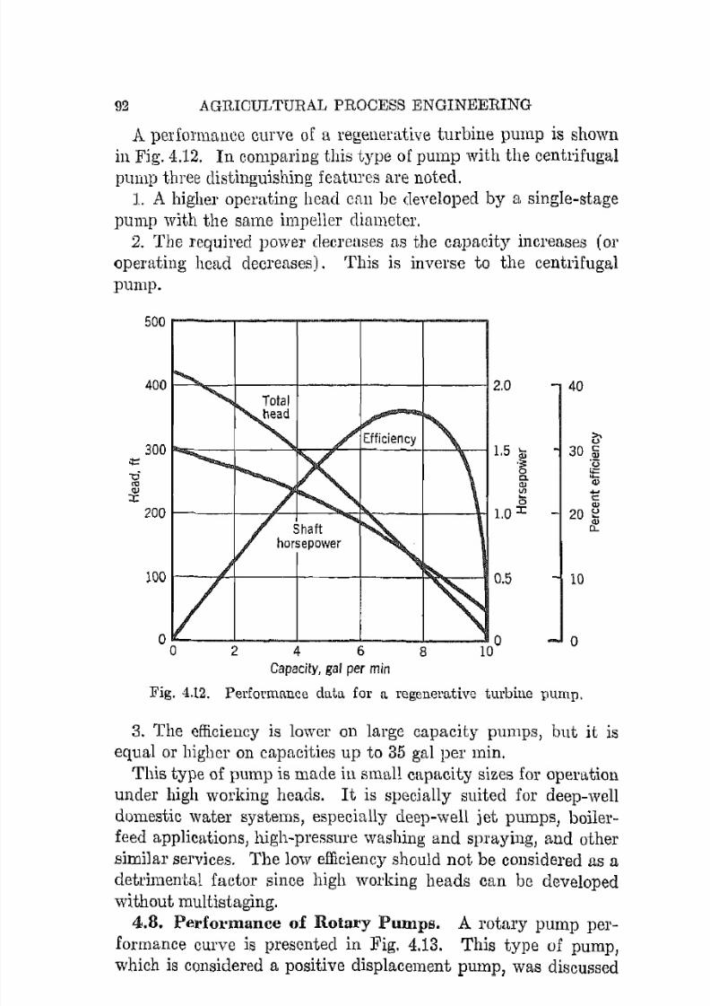
7/16/2019 Engenering Agriculture Perry
http://slidepdf.com/reader/full/engenering-agriculture-perry 101/422
92 AGRICIDJTURAL PROCESS ENGINEERING
A perfOl'lllfl,llee curve of a regenerative turbine pump is shown
in Fig. 4.12. In comparing this type of pump with the centrifugal
pump three distinguishing features are noted.1. A higher operating head can be developed by a single-stage
pump with the same impeller diameter.
2. The required power decreases as the capacity increases (or
operating hcad decreases). This is inverse to the centrifugal
pump.
5 0 0 ~ - - - - T - - - - - ~ - - - - - r - - - - - T - - - - ~
2.0 40
3 0 0 ~ ~ - - + - - - ~ ~ - - ~ ~ - - - - ~ - - ~ ~<t:
")6-
:J!2 0 0 ~ - - - - + - - - ~ 4 - - - ~ ~ ~ - - - + - - - - ~
t;-1.5 ~ 30 fi3
.:: ·u0 :t:"'-til tilII I .....(5 t :
'".0
J :20 ~C>-
0.5 10
2 60
4 8Capacity, gal per min
Fig. 4.12_ Performance data for a regenerative turbine pump.
3. The efficiency is lower on large capacity pumps, but it is
equal or highcr on capacities up to 35 gal per min.
This type of pump is made in smtl11 capacity sizes for operation
un.der high working heads. I t is specially suited for deep-well
domestic water systems, especially deep-well jet pumps, boiler
feed applications, high-pressure washing and spraying, and other
similar services. The low efficiency should not be considered as adetrimental factor since high working heads can be developed
without mUltistaging.
4.8, Performance of Rotary Pumps. A rotary pump per
formance curve is presented in Fig. 4.13. This type of pump,
which is considered a positive displacement pump, was discussed
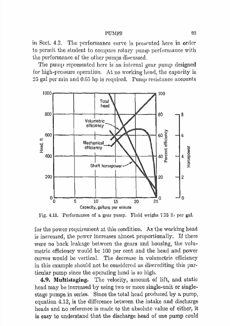
7/16/2019 Engenering Agriculture Perry
http://slidepdf.com/reader/full/engenering-agriculture-perry 102/422
PUMPS fJ3
in Sect. 4.2. Tlle performance curve is In·c,;pnted hero ill order
to permit the student to compare rotary pump performallce with
the performance of the other ]lumps dit-'cussed.The pump represented here is an illtcrnal gear pump designcd
for high-pressure operation. At no working hearl, the capacity is
25 gal per min and 0.05 hp is required. PUlllP resi;"tancc accounts
1000 100
800 80 8
>.
600u
60 :ii 6~ ·u"t:i ~'"
OJ ~'" - <l)
:t: c: ;::
400<l) 0
40 ~ 4 Q.,QJ
'" ~..
::t:
200 20 2
00 5 10 25°
015 20
Capacity, gallons per minute
I<'ig. 4.13. Performance of a gear pump. Fluid weighs 7.75 Ib pel' gal.
for the power requirement at this condition. As the working hearl.is increased, the power increases almost proportionally. I f there
were no back leakage beLween the gears and housing, the volu
metric efficiency would be 100 per cent and the head and power
eurves would be vertical. The decrease in volumetrin efficiency
in this example should not be considered us cliRnrediting this par
ticular pump since the operating head it> so high.
4.9. Multiataging. The velocity, amount of lift, and static
head may be increased by using two or more single-unit or singlestage pumps in series. Since the o t i ~ l head produced by a pump,
equation 4.13, is the difference between the intake and discharge
heads and no reference is made to the absolute value of either, it
is easy to understand that the discharge head of one pump could
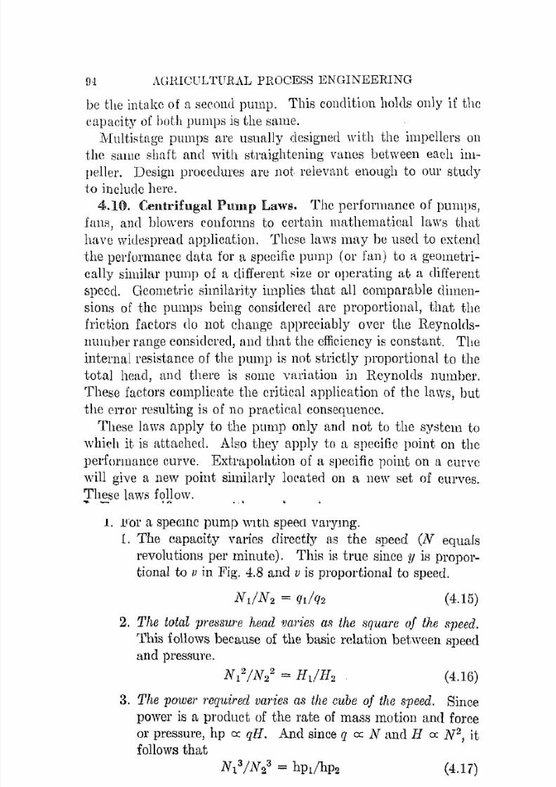
7/16/2019 Engenering Agriculture Perry
http://slidepdf.com/reader/full/engenering-agriculture-perry 103/422
!H AUmCULTURAL PHOCESS ENGINEERING
be the intake of a second pump. This condition holds only if the
capueity of buth pUlllpS is the same.
Multistage pumps arc usually designed with the impellers onthe sallie shaft and with straightening vtlnGS between eaell im
peller. Design procedures are not relevant enough to our stuely
to include here.
4.10. Centrifugal Pump Laws. The perfonnance of pumps,
fans, and blowers conforms to certain mathematical laws that
have widespread application. Thcse laws may be used to extend
the performance data for a specific. pump (01' fan) to It geometri
cally similar pump of a different size 01' operating at a differentspeed. Geometric similarity implies that all comparable dimen
sions of the pumps being considered are proportional, that the
friction factors do not change appreciably over the Reynolds
number mnge considered, and that the efficiency is constant. The
illternalresistance of the pump is not strictly proportional to the
total head, and there if; some variation in Reynolds number.
These factors complicnte the critical application of the laws, but
the error resulting is of no practical consequence.These laws apply to the pump only and not to the system to
which it. is attached. Also t.hey apply to it specific. point on the
performance CUl've. Extrapolation of H specific point on a curve
will give a new point similarly loeated on a new set of curves.
These laws follow.
T. For a specific pump with speed varying.
1. The capacity varies directly as the speed (N equals
revolutions per minute). ThiR is true since 11 is propor
tional to /) in Fig. 4.8 and /) is proportional to speed.
(4:.15)
2. The total p l ' e ~ s " U r e head varies as the square of the speed.
This follows because of the basic relation between speed
and pressure.
(4.16)
3. The power requ'ired varies as the cube of the speed. Since
power is a product of the rate of mass motion and force
01' pressure, hp a: qH. And since q ex Nand H 0 : N 2, it
follows that
(4.17)

7/16/2019 Engenering Agriculture Perry
http://slidepdf.com/reader/full/engenering-agriculture-perry 104/422
PTTl\lPS
Ex I Illl'h>. A PUlilp. upel:li llH.( at 17(j1) ljJlll, df,lh ( ling 12,j gal IWI' min
at 1O ft of hpo.ri, and leqlllring 10:\ hOl 'f 'J 'Ol\PI. 19 "1"pp,jl'll up to 2100
rpm. \VhaL alP thp l l P ' ~ 0lWtaimg rOlldlt\()n,'; 1'hp l'llJl.l.eity, equation4.15,
1760/2100 = l25/1]2
= 1·10 [.!;lll pel' min
TIll' total head Pl'OdlWl'ri, ('f[u!ltion 4.10,
17lilj2(21002 = 4 ( ) ' H ~][ 2 = 5B ft,
The pa l l "I' lPquil'ed, ('quai iOIl 1.17,
17(\03 i21003 = l.li3/ p ~hP2 = 2.71l
(Note' thtlt, I w c a u ~ e of ,imiiadty, the new operating p o ~ i t i ( ) I l iR at till ' ,,!1I1IP
l'plativp po'oition I'Pgal'ding pflici('nry the initialojlPlaiillg pniut)
U. For a numher uf geometri(,ally similar pumps with fiprccl
(lonstant, and climneter varying.
]. The capacity varies a8 lhe wbe of the diameter. The
e[1pacity is a dire(,t lunetion of pcriplwl'Y speed ~ t l l dperipheryarmL. Since the periphery speed varies directly
us the diameter and the area ab the> Rquare of the dimneLer, it follOlYS that
(-U8)
2. 'rhe head v(Lries ag the 8QU(L1'1! of the dialHfi(')'. The p1'OS-
8me varies as the SqlWI'(' of the veloeity. The velocity
of the fluid leaving the impeller varies us the diauwterof the propeller, consequently,
(4.19)
3. The ]lOWe!' l1atie!; as the fifth power of the diameter. SincE'
power is the product of quantity discharge and head,
equations 4.16 and 4.17 combined in product show that
(-1:.20)
Example. A pump with a 7-in. runner delivers 125 gal prr min againsL
0. 40-ft head and requires 1.63 hp. I f the "peed is maintained constant
ami th e runner diameter increased to 7.42 in. (because of similarity, all
7/16/2019 Engenering Agriculture Perry
http://slidepdf.com/reader/full/engenering-agriculture-perry 105/422
96 AGRICULTURAL PROCESS ENGINEERING
linear dimensions would be increased proportionally), what are the new
operating conditions?
The capacity, equation 4.18, is
q2 = 140 gal pCI' min
The total head produced, eqUlttion 4.19, is
72/7.422 = 40/112
IIz = 45 f t
The pOWel' req_uired, equation 4,20, is
75/7.42" = l.63/hp2
hpz = 2.18
(As ill the previous example the new operating point bears the saIne relat,ion to the new efficiency curve as the initial point bears to the initiuJ
efficiency cUl've,)
Note that the two examples were taken from the performance
data of Fig. 4,9. The capacity or rate of discharge was raisedfrom 125 to 149 gal per min first by increasing the speed of the
runner from 1760 to 2100 rpm and then by incl'ettsing the diameter
of the runner, Although the rate of discharge was the same in
both instances, the total operating head resulting from the speed
increase was 56 ft, but that resulting from runner-diameter in
crease was only 45 ft, Comparable variations in power require
ment are noted.
These variations would lead one to believe that any head between 45 ancl56 ft could be produced by adjusting both speed and
diameter. Fortunately, a procedure is available for extending
performance data to any desired condition from any operating
point on a performance chart.
The development of this procedure follows:
The pump laws may be combined so that the speed and di
ameter effect appear in the same equation, thus:
ql/q2 == (JV 1/lV2)(1)13/1)23)
HdH2 = (JV12/JV2
2)(D12/D22)
hpdhp2 = (JV13/JV23)(D15/D25)
(4.2!J
(4.22)
(4.23)

7/16/2019 Engenering Agriculture Perry
http://slidepdf.com/reader/full/engenering-agriculture-perry 106/422
PUMPS 97
By solving equations 4.21 and ·1.22 simultaneously, the folluwinggeneralized exprpCisiollf, are secured.
D2 = D l ( I I / ~ ! q l ~ j ) ( q l ! J I I I 2 J " )N2 = N l ( I I l ~ 5 . / H l H ) ( I I 2 Y . / q 2 ' 2 )
(4.24)
(4.25)
'rhe application of these most important e x p r r s ~ i o n s and of
equation 4.23 are demonstrated hy the following eXl11J1ple.
Example. A pump is Lo he selcrted oilllilar to the Pllmp of l?jg. 4.9 to
deliver 75 gal per min against [ l 05-ft head. I t is desirable to operate it at
11 point on it s performance curve compmable to the 150-gal-per-min point
on the base curve, Fig. 4.9. The basic conditions are 150-gal-per-min cu
pacity, 36-ft head, 7-in.-dinmeter Tllllner, and 1760 rpm. They are ql' HI'
DI , am! N l , resprcth·cly. The required runner diameter from equation4.24 is:
The rcquin'd runner speed from equation 4.25 is:
The paWN' ]'equired elm be calculated from cquation·1.23, which, tranoposed,
iR
or,
hP2 = l.G3(38703/17G03)(4.285/7") = 1..18
In equations 4.23, 4.24, and 4.25 the subscript-I values mustbe taken from performance data for the basic pump and any subscript-I value fixes all the oiher sUhscript-l values. SUbscript-2values are not so fixed and may vary at random.
H in these equations is defined as total head in feet of fluid.Since these equations are based on geometric similarity and the
terms are in ratio in each equation, H can be expressed in anyconvenient dimension, such as inches of mercury, inches of water,
pounds per square inch, and can represent static hcad or pressure
or velocity head as appropriately as total head.4.11. Pump Performance on a System. The system to
which a pump is attached could be made up of lengths of pipe,valves, various joints, orifices, transitions, etc. The sum of theresistances of the various elements, the elevation or fluid lift,
and the velocity pressure head is the total head, which can be
calculated by the Bernoulli equation (Sect. 2.6). A graph of
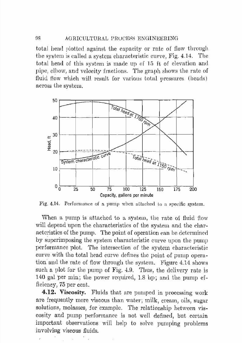
7/16/2019 Engenering Agriculture Perry
http://slidepdf.com/reader/full/engenering-agriculture-perry 107/422
OS AGRICULTURAL PR(JCEHS ENGINEERING
total 11ea(l plotted against the eapacity or rate of flow through
the system is called a system characteristic CUl've, Fig. 4.14. The
total head of this system is made up (if 15 ft of elevation and
pipe, elbow, and velocit.y fractions. The graph shows the rate of
fluid f l ~ w which will result for varian;,; total pressures (heads)
across the system.
25 50 75 100 125 150 175 200
Capacity, gallons per minute
Fig. 4.14. Performance of It pUlllP wben a t t : l e h l ~ d (0 l1 specific systelll.
When a pump is f\ttached to a system, the rate of fluid limv
will depend upon the characteristics of the system and the cital'
nctcrist,ics of the pump. The point of operation ean be determined
by superimposing the system eharacteristic CUrve upon the pumpperformance plot. The intel'seetion of the system characteristie
curve with the total head curve defines the point of pump opera
tion and the rate of flow through the system. Figure 4.14 shows
such a plot for the pump of Fig. 4.9. Thus, the delivery rate is
140 gal per min; the power required, 1.8 hpj and thc pump ef
ficiency, 75 per cent.
4.12. Viscosity. Fluids that are pumped in processing work
are frequently more viscous than water; milk, cream, oils, sugarsolutions, molasses, for example. The relationship between vis
cosity and pump performanee is not well defined, but certain
impOliallt observations will help to solve pumping problems
involving viscous fluids.
7/16/2019 Engenering Agriculture Perry
http://slidepdf.com/reader/full/engenering-agriculture-perry 108/422
PUMPS
The efficiency of a pump clec'rea:>c;,j a:-; the yisco;;ity illCrCa;-;e:-i.
The illCl'OlLt-Jed fluid friction betwr:en the pump part;;~ U l d
thepassing fillill uncI between pump part::) Acpnratl'd by fluid cli:3-
:-;ipntcA lllUl"l" llleclmnical ellergy [ l " heat ellergy, and l e s ~ of tho
:-;haft input energy iA uyailable to do ll!'eful work. I t llotpoE,l-lihle to pruyide a gencrnl correction prucedure for the erfed
nf vjEl('oBity n1)U11 effkicney "inca the 1m;,; in tile !JUlEp is llue tohydraulic. frictioll anLl lllcc-iwnil'al fridillll, whi('h arc not gell
erally related.
The w o r k i n ~ head incrcases a,; the yi:-;l'lIsity illrrea"c;;.
Reynold:; numher, equation :2.(j, v:tril'''; inver:-;ely as 1,l1e v i : . : c o ~ i t : > ' .Since a large Reynolds muuber is desired for mOnt, :omti:-;factory
perfOrlllUlH'O, fluids of high vibr'osity mtlllf, he moved in lal'ge
diameter pipes in order to minimize frietinn head lOlil3os. The
rate of flow cau he rcducC'd to produc:e [t further l'cduetion in
hC'atlloss.
REFERENCES
1. Abramson, 11. L. Pf'rform:tIH'e Chllraeit'rislic:'l of 'furLin" Pump;,; at
3500 and 1 7 . ~ 0 rpm. PI /WIT lll:3lJO-301. l\hy, 1947.
2. Addison, H . .1l'mlllise Oil Applied 1IIJ,zrulllil".·!. Thir,l Edition. Wilpy.
1945.3. Church, A. ll . Centrifu(lill Pllmps 1111(1 Blowers. ,Viley. 1014..
'1. Gosline, .r. K, llud O'Bricn, ]1.1. P. The W,11.er JPL Pump. Unilrersityof
California Puhlication in EnglUCPl'illg 3: 167-HlO. l!J34.
5. H ydmulic Inslitutc Tcst Cor/e, Cl'ntrij1I(lrll Pllmps, Section F. Hy
draulic Institute. 1036.
6. Perry, J. H. C'ltcmical Enoinl'efin(J IIandlwuk. l\IeGrmv-Hill. 1934.7. ' l ' [ ' ~ t (}ode jor Centl'ijll(Jal (Iud Rotary Pllmps Powl'r l'C8t Code.<.
A.S.IV1.E. 1927.
PROBLEMS
1. A who!£' milk homogenizer operating at a l'r(';.sure of 2500 sq ill. dr.
liYers 6 gal l)el' min. I f tllr pump efficiency is 82 pe!' cent, what si7.('
mutor iH req1lired'l What siz,' motor lWllliret[ if t lip p r e ~ 8 u r e is 1500 III
pel' sq in.? Pipe friel ion may be nrgJec·1ed. E ~ t i l l l a t o t h f ~ Yelol'ity
thl"Ough the homogenizing valve.2. A 1750-rpm ('('nlrifngai pump with a 4.7:j-in. impeller ll(lliyf'l's 140 g:d
]Jcr min agaillnt, a 20-ft water hf'afl and uses 1 hlWSPj)mver. \VIJllt is tlw
pump efficioncy? What i::; the head at, cOlupif'te Hlmt-off?
3. The jJump of problem 2 is to ojJcratf' against (I 25-ft head without clutng
ing officieney. Spceify tho ~ p e P l l , dischargr rate, and power reql1ired.
7/16/2019 Engenering Agriculture Perry
http://slidepdf.com/reader/full/engenering-agriculture-perry 109/422
100 AGRICULTURAL PROCESS ENGINEERING
4. The pump of Fig. 4.9 is connected to ,10 ft of 2-in. galvanized-iron pipe.The lift; is 25 ft. The system contains 2 elbows, pumps from a tank,
and discharges from the pipe. What is the water pumping rate?5. Specify a pump geometrically similar to that of Fig. 4.0 to operate at
maximum efficiency at a head of ·10 it [\nci cap[\eity of IS!] gal pel' min.Impeller diameter, speed, and horsepower [\1'C rcquired.
6. Determine the efficiency of the pump of Fig. 4.111 when operating at1150 rpm.
7/16/2019 Engenering Agriculture Perry
http://slidepdf.com/reader/full/engenering-agriculture-perry 110/422
C H A P T E R 5
fans
NOIUENCLATURE
D = diameter, in.
TI = total head, ft.N = revolutions per minutp.
P = fan pitch, ft pel' rev.q = air rate, ell i t per min.l' = m d i u ~ , ft .a = fan-blade lLngle of twist, degrees.'Y = specific weight, Ib per ell ft.
Fans are used in agricultural p r U l ~ e H s i n g in connection with
drying, ventilating, heating, cooling, refrigerating, aspirating,
elevating, and conveying. Processing and other agriculturalactivities rcquiring fans is increasing. Costs are becoming more
:;1nd more important, and it is necessary that the processing en
gincer be able to select and apply the best fan for any installation,taking the economic factors into consideration.
The terms fan, blower, compressol', etc., are frcfJ_uently used
interchangeably, The American Society of Mechanical Engineers 6 ,7 has placed these devices into the following classifications:
Class I, Compressors. Operate at pressures equal to or morethan one Ib pel' sq in. (27.7 in. of water). Machines in this classare also called centrifugal compressors, turbo compressors, and
blowers.Class II, Fans. Operate at pressures of less than one lb per
sq in. (27.7 in. of water). Machines in this class are also called
centrifugal fans, fan blowers, or exhausters.This classification was developed to expedite testing, the main
difference between classes being the fact that, the heat of C O l l 1 p r e s ~sion and the variation in specific weight must be recognized andconsidered in Class I whereas in Class II it is of minor importanceand may be neglected in most tests. Compressors are usually
applied to an agricultural processing job as packaged units such
101

7/16/2019 Engenering Agriculture Perry
http://slidepdf.com/reader/full/engenering-agriculture-perry 111/422
102 AGRICULTURAL PROCESS ENGINEERING
as nil' or refrigeration compressors. Consequently, a detailed
treatment of compressors is not important in this book. Fans
will be discussed sinr:e they must be selectc(l, adapted, and per
lwps designed for spec:ifie installations.
Fans may be classified <-IR to type or design according to the
following schedule, which is recognized by the National Associa
tion of Fan Manufacturers."
5.1. Axial·Flow or Propener Fans. In this type ail' flow is
parallel to the shaft or axis. Propeller fan is a generic term.
Technically axial and propeller fans are the same; past experi
ence and general usage, however, !tIWl: segregated the duties for
which eueh fan is used.
5.2. Propeller Fans. This type may have two or more blades
whieh may be of shect steel or airfoil shapo. The blades may be
narrow or wide. They may have uniform or varied pitch. This
type of fan, sueh as shown in Fig. 5.1, has been developed and
used to handle large yolull1eH of air against free delivery or low
heads.
Fig. 5.1. A propeller fan. (Courtesy Hartzell Propeller Fan Co.)
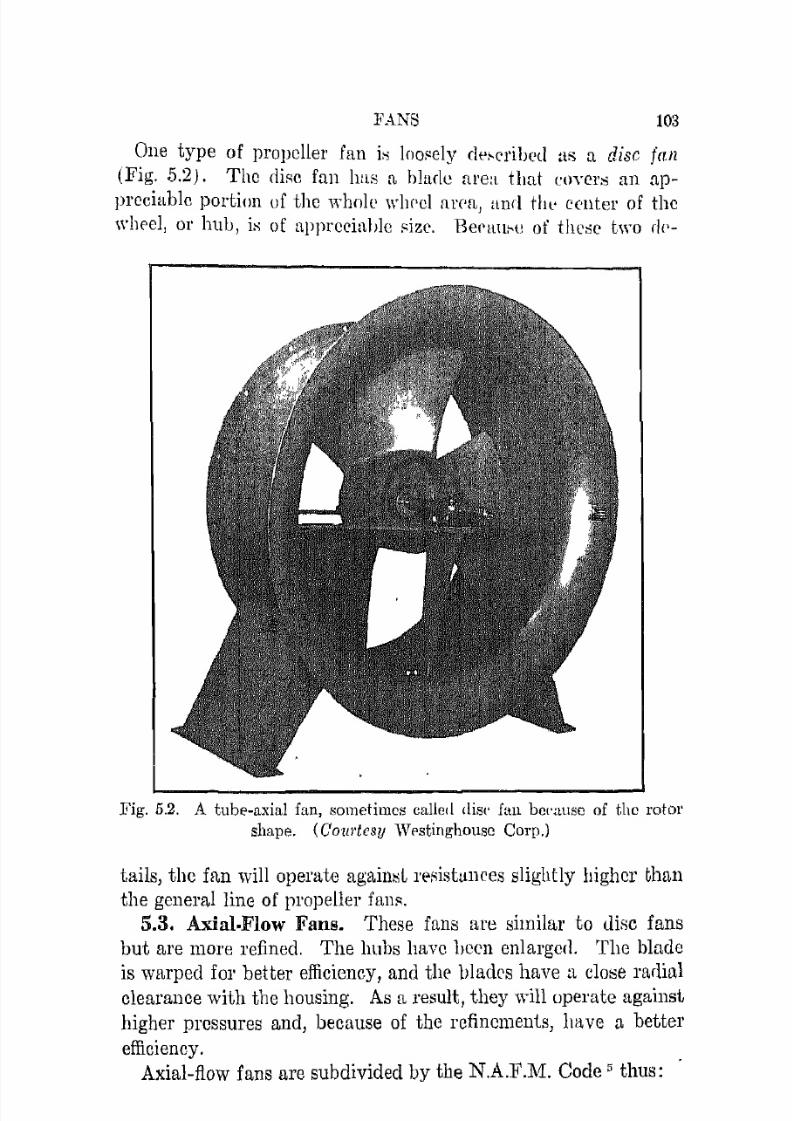
7/16/2019 Engenering Agriculture Perry
http://slidepdf.com/reader/full/engenering-agriculture-perry 112/422
leANS
One type of propeller fan i" I ( ) o ~ e l v d t ' ~ ( ' r i b ( ' d as U disc fan(Fig. 5.2). The diRe fUll has n, h l l l d ~ area tlmt toyers nn ap
preciable portion uf the whole ,,"lweI area, and thL' center of thewheel, or hub, i" of appreciable "ize. Be!'au:-u of t h ( ' ~ c L\YO fIP-
Fig. 5.2. A tube-axial fan, sometimes called dis(' Jan bC(';tuSC of the rotorshape. (Coll1'tesy WrstinghotIsc Corp.)
tails, the fan will operate againtiL l'l'Ristul1ces slightly bigher than
the general line of propeller f a n ~ .5.3. Axial.Flow Fans. These fans are similar to !lise fans
hut are more refined. The huhs have hern enlargc(1. The blade
is warped forbetter
efficiency, and tIl(' bladeshave
a closeradial
clearance with the housing. As a result, they will operate against
higher pressures and, because of the refinements, ha.ve a better
efficiency.
Axial-flow fans are subdivided by the N.A.F.M. Code:; thus:

7/16/2019 Engenering Agriculture Perry
http://slidepdf.com/reader/full/engenering-agriculture-perry 113/422
104 AGRICULTURAl" PROCESS ENGINEERING
5.4. Tulle·Axial Fan. leA tube-axial fan consists of an axialflow wheel within a cylinder and includes driving-mechanism sup
ports either for bclt drive or direct connection," (Fig. 5.2.)5.S. V nne.Axial Fan. "A vane-axial fan consists of an axial
flow wheel within a cylinder, a set of guide vancs located either
Fig. 5.3. A vane-axial fan. Note the guide vanes behind the fan. (Cour
tesy The Buffalo Forge Co.)
before or after the wheel, and including driving-mechanism supports for either belt drive or direct connection." (Fig. 5.3.)
5.6. Centrifugal or Radial-Flow Fan. This type is shown inFig. 5.4 and consists of a wheel 01' rotor within a scroll spiral type
housing. The air enters parallel to the shaft, makes a 90° turn

7/16/2019 Engenering Agriculture Perry
http://slidepdf.com/reader/full/engenering-agriculture-perry 114/422
FANS 105
Fig. 5.4. FOl'wal'd-curved-blade and backward-curved-blade centrifugalfans. (Co1!1'tesy Westinghouse Corp.)
in the fan wheel, and is discharged from the wheel ([lnd housing)
in a radial manner.Centrifugal hns can be subdivided into the three classes shown
in Fig. 5.5, which are tliscussed in the follO'wing sections.
Forward curve Straight Backward curve
Fig. 5.5. The three types of centrifugal fan rotors, with velocity diagrams.
5.7. Type a, Forward-Curved·Blade Fans. This type has arotor similar to a squirrel cage and a large number of blades,
i.e., up to 60, narrow in the radial dimension but wide parallelto the shaft and facing forward in the direction of rotation like
7/16/2019 Engenering Agriculture Perry
http://slidepdf.com/reader/full/engenering-agriculture-perry 115/422
106 AGRICULTURAL PROCESS ENGINEERING
a scoop. I t is a low-speed fan, capablc of operating at several
inches p r e ~ s u r e under most conditions but is limited to handling
deun air.5.B. Type b, Radial.Tip Straight or Double.Curved.Blade
FmD.8. This type has a smaller number of blades-from fi to 20 -
and the hlndes ure essentially in a plane radiating from the shaft.
The blades fire l101'1l1nlly about 2 t.o 3 times as long radially as
Lhey are wide. This Lypc of fan usually has a larger housing than
the other tYlleH and is more expensiYl;; however, its priee is justi
fied by its ability to handle dirty ail' and to convey materials that,
go through the fan or to develop pressures beyond the range per
missible with lighter weight fans.
5.9. Type c, Backwurd·Curved·Blade Fall. This type has
ahout 12 blades, essentially flat and tilted backward from the
direction of wheell'Otatioll. I t is inherently a high-speed type of
fan ,,,ith a self-limiting horsepower characteristic (Sect. 5.12).
I t is the most eHiciellt. of the various types of centrifugal fans and
11lO1'e expensive than the otJler types. Size for size, however, it
has cOlll]larable effieiency and cost. "With t.he added feature of
[,he sdf-Iimiting horsepower eharaet.el'istie, it. is the best selection
for reasonably clean air. I t C;l11l1ot as yet be recommended for
rJirty nil'.
FAN THEORY
The propeller fall is essentially an air screw. The t.\vist or
angularity of the blalleR is called "pitch," and theoretically it is
the distance the ail' would be moved when turning the rotor 1 rev.
I f C( is t.he angle of fan-blade twist, the "piteh" at any cross sec
tion at a distance r from the axis is
P = 27ri' tan a (5.1)
Note that the pitch increases as the radius for a fan with a con
st.ant blade twist or angUlarity. Consequently, the air near the
{,ip of the 'fan is being moved at a faster rate than the air nearer
t.he axis, the speed being theoretically proportional to the clis
tance,frql11 t.he axis. Therefore, when the fan is operating against
H. material static head, ail' is forced back through the fan ncar the
hul} a n { l l ' ~ e i r c u l a t i o n or turbulence occurs as shown in Fig. 5.fi
and lowers the efficiency.

7/16/2019 Engenering Agriculture Perry
http://slidepdf.com/reader/full/engenering-agriculture-perry 116/422
107
Recirculation can be reduccd 01' ciinllnated by warping tllP
bladeR so that the llltch i" c O l l ~ t a n t The Wlll'[I' (k:.. ~ n cun 1)('
determined from equatlOll 5.1 by hnillinl!; P eon:-.tant and uetf'l"mining IX for variation in r. A large htrertmlinrd hub fl.') ShOWI1 III
Fig. 5.3 improves pedormaJll'e hy chlllinating the rq;ion of rc
CIrculation. A rylinclrirnJ housing illlpronl> llPrforrnallce by guid-
FIg. 56. Recil"lulatJOll tlMt re"ult9 WlWll ]1lojlellol" n I <IN' fan IS Opel[l.tpo]
a g l l i n ~ t too great tl slahl' hf'ucl.
ing the stream of air that passes through the fan. The perfor
mance and efficiency of the ~ t x i a l - f t o w inn can be further improved
by the addition of straightening, valles behind the rotor. The
discharge from a "propeller" fan it, in the form of a :-,piral, the
rotation being in the samr dircdion H:O; the rot.ttiUll (If the fan
wheel. Straiglltenmg vanes catel! the air, turning it so it;; fl()w
i::; parallel to the shaft. Elilllination uf turbulcnc'c l'ednees noi;;e
and improves the effiriency. Straightening v a n e ~ ,,}lould be 2 to
4 in. from the blade wheel to minimize noise.
Pressures in excess of 60 in. have been developed by a single
axial-flow fan, with a total effiCiency of more than R5 per cent.
Centrifugal fan theory parallels that of centrifugal pumps (sect.
4.5 and Fig. 4.8) and will not be discussed here. However, C011-

7/16/2019 Engenering Agriculture Perry
http://slidepdf.com/reader/full/engenering-agriculture-perry 117/422
108 AGRICULTURAL PU.oCESS ENGINEERING
sider Fig. 5 . ~ which shows the three general types of centrifugal
fan wheels in view of the centrifugal pump theory. Consider thevelocity diagrams of the three general types shown in Fig. 5.5.
FOl' a constant peripheral speed, observe that the discharge ve
locity V for the forward-curved fan is approximately three timesas great as for the backward-curved fan. Considering equation
4.13, note that the static pressure produced by the forward-curvedfan is very small when compared with the backward-curved unit.
This characteristic is outstanding as regards centrifugal fans andwill be discussed in the following sections.
PERFORMANCE
5.10. Axial-Flow Fans. Fans are tested and rated on the
basis of the Test Codes of the American Society of Mechanical
a : r 8 o , _ - t - ~ , , = - t - - t - - ~ ~ E ~ ± : = - + - - + - - - j8~ 6 0 ~ ~ - - - r - - + - ~ ~ ~ - - ~ ~ ~>E'x
! 0 r - - - ' _ - - - + ~ ~ - - - - ~ - - ~ - - - 4 - - - - ~ ~ ~ ~ ~ __:3
~ 2 0 r - - - ~ ~ - + - - ~ ~ - - + _ - - ~ - - _ 4 - - - - ~ - - ~ - - ~ - - ~
10 20 30 40 50 60 70 80 90 100Per cent wide-open capacity
Fig. 5.7. Representative axial-flow-fan performance curves expressed on a
percentage basis.
Engineers,6.1 using the same procedure as discussed for centrifugalpumps in sect. 4.6.
A characteristic perfonnance curve for an axial-flow' type ofpropeller fan is given in Fig. 5.7. The reversal of the power andhead ClU've is characteristic of propeller-type fans, although it is
more pronounced in some particular makes. The point of reversal indicates the limit of stable operation of the fan. As a
general rule, the power curve is relatively fiat, especially within

7/16/2019 Engenering Agriculture Perry
http://slidepdf.com/reader/full/engenering-agriculture-perry 118/422
FANS 100
the practical opel'aLing runge, say above 40 per cent of wide-open
capacity. When this rule does not hold, the power may decrease
toward the wide-open capacity and increase near the point ofcomplete shut-off. Undel' such conditions, the power requirement
increases when the fan is throttled, owing to greater resistance
head and l unless extra power is available for this contingency
the power unit may be overloaded and difficulties may result.
I t is generally advisable to assume that the power increases as
the capacity decreases, although the rate of increase may be small
and a reversal in the power curve usually exists.
5.n. Forward-Curved-Blade Fan. Fans of this type can beused for installations where the operating conditions are rei a-
w w ~ ® ~ 00 ro mPer cent wide-open capacity
Fig. 5.8. Representative forward-curved-centrifugal-fau performance curvesexpressed on a percentage basis. The power curve is bnsed upon the maxi
rounl rather than the closed value.
tively constant, static heads are low, and the air or gas is clean.
Since the discharge velocity V is high, operating speeds can be
low and the fan size small.
The performance characteristics of a forward-curved fan are
shown in Fig. 5.8. Note that (1) the maximum efficiency occurs
at 40 per cent wide-open capaoity; (2) there is a complete re
versal of head curves; and (3) the power requirement increases as
the capacity increases.
Three ca.pacities or ratcs of discharge are possible at the same
static head. I f the fan i.s connected to a system with a system

7/16/2019 Engenering Agriculture Perry
http://slidepdf.com/reader/full/engenering-agriculture-perry 119/422
110 AGRICULTTTRAL PROCESS ENGINEERING
characteristic curve passing through this area, hunting may result
between these three points.
The increase in power that develops as the capacity increasesIllay be disadvantageous, since the motor might be overloaded
when decrcasing the SYHtClll resistance.
In spite of the above-implied disadvantages, the forward-curved
fan is suitable for ventilation and ail' conditioning jobs where the
operating conflitions arc constant and thc air is clean.
5.12. Backward-Cul'ved Centrifugal Fane. The performance
of this fan is compamble to the centrifugal pump sinee the design
is similar.
Per cent wide-open ca pacity
Fig. 5.9. Hepresentative backwal'd-CUl'ved-centl'ifugal-fan performance
eUl'ves expres8f'd on a percentage basis. The power curve is based on the
maximum l'nthel' than the closed value.
Note from Fig. 5.9 that (1) the maximum efficiency occurs at
!l.bout 60 PCl' ccnt wide-open ct'lpacity; (2) the head curve in
creases fairly consistently from wide-open capacity to nearly coUl
plete shut-off; and (3) the power curve is a maximum at a point
nearly coincident with the maximum-efficiency point.
The rising pressure curve practically eliminates the possibilityof hunting. With the maximum in horsepower occurring at ap
proximately the same point as the maximum efficiency, it is
possible to pick the fan with peak efficiency and be unable to
overload the motor by either increasing or decreasing the pressure
or eapacityas long as the .speed is constant.

7/16/2019 Engenering Agriculture Perry
http://slidepdf.com/reader/full/engenering-agriculture-perry 120/422
F A N ~ 111
Thc hackwlwl-l'Ill'V('(l-IJIltdc fnn opcl'alP,., at niJollt 1.7.3 to 2.0
times the SPCC(\ of Lhc fOl'\\'al'd-wl'\'ed-bladr fan of (·olllparahlc
size and capacity.
5.13. Straight.Blade Fans. Their pCl'lonnancl' i" ",illJilar 111
the forwt1nl-curvc<l-hla<lo fun in that th('y ]lrIYe a ribing ilOtH!
power ourve, although there it:- 110 complete r l ' v e ] ' ~ a l (If tht, Pl'l';-,.,;urc
curve. The cffiei('l1cy is about the same. Air wlol:itic" thrullgh
Lho wheel and in til(' l l O u ~ i n g arr' lnwer, at'; thl' fan mudt Inl'gl'l'.
This fan wa:; tlw firRt to be wwd ill Jlllhlir lJllilding"'. When pi('};:cri
for peak efficiel1ry, it is very quil't, hut owing to ib f,izl' it iH abo
quite expensive.
Its Ui:iC is now limited to pneumatic l:llllccting or eUll\'cyillg
where material must go through the fan or where tILe fan lllUst
handle dirLy air or gas.
5.14. Combillation.Curved.Blade Funs. Thill type ('uvers
fan blaclei:i of VariOlli:l :-hapeF:. BOllte \yitiJ forwltrd-('Ul'Vell pntpring
edges, SOUle with backward-curved leH\'illg erlget), anll !lume with
combinations of radial sections.
Generally, theHe fanH have pcrfOl'lllanep eUrycs :;imilnJ' tu the
forwarc[-rl\l'vec[ OJ' stmigbt-bla[le fall:---that is, they han' ri::;ing
horsepowl'r rharactcristics an[l peak efilcicllcies lowpl' than t h o ~ I 'a\'ailable wiLh the backward-curvet! hlurle.
5.15. Factors Affecting Fan Selection. The fullowing infu1'
mation mU8t he known when selecting a fan, These factor" aid
in determining the type of fan to be selected and the . ~ j z c .
1. (-luantity of air to be moved pur ullit of time.2. Estimaterl l'lystell1resistallee and expected variatium'.
3. Amount of noise perlllitted.
4. Space available for fan.
5. Economic implications,
The quantity of air to be moved per unit of time will be deter
mined from the type and size (Jf installation and will not he
d i ~ c u s s e c l here.The static pressure drop or resistance head can be determined
conventionally by methods diseusserl in Chap. 2, Fluid Mechanics.
Note that each type of loss, pipe friction, turns, valves, entrance,
outlet, porous media, etc" varies nearly as the square of the
velocity. Therefore, the total resistance 01' static pressure js

7/16/2019 Engenering Agriculture Perry
http://slidepdf.com/reader/full/engenering-agriculture-perry 121/422
112 AGlUCULTURAL PROCESS ENGINEERING
nearly a square function of the velocity through the system.
Curves A, B, and C on Fig. 5.10 are slIch curves for three different
systems and are called system characteristic curves. For example,system B requires a static pressure of l.'115 in. water to deliver
1.8
a
1.6
Total
1.4
1.2 3.0
:u':t1
1.0 2.5;:
~ 0.8 2.0<1l
0: ~Q)
;;:0.6 l5. 1.5
Q)
!.'!0:c
0.4 1.0
0.2
02 4 6 8 10 12
Volume, 1000 efm
Fig. 5.10. Pei'fOl'mance curves of a backward-curved centrifugal fan show
ing system chal'actel'isties.
8000 cu ft of air per min, but the static head would be only 0.8
in. water if 6000 eu it per min were being delivered. The total
pressure, power requirement, and efficiency are located on line
b-b. The importance of thesc curves will be discussed in Sect.5.16.
Noise is not as important a factor in processing work as in air
conditioning or household ventilating, but since excess noise may
indicate a significant loss of energy, noisy operation should be
minimized as much as practicable.

7/16/2019 Engenering Agriculture Perry
http://slidepdf.com/reader/full/engenering-agriculture-perry 122/422
FANS 113
There are usually a number of fans that will fulfill the require
ments lor a specific job. A large expellsive flm operating at l)cak
efficiency or a smaller, higher speed, less expensive, and less efficient fan will do a certain job, for example. Which to select
will depend upon the amount of u:::e, stability of use, an,l c o ~ t of
power. Chap. 13 on cost anulysi::; will aiel in solving such problems us these.
5.16. Fan Selection. The syst.Cll1 characteristic of a specifled
installatioll is curve B ill Fig. 5.10. Eight thousand eubic feet
of ail' pel' minute must be deliverer!' Consequently, the stlttic
operating head will be 1.41 in. of water. Significant variations inoperating conditions are not expccted.
I f the factors causing resistance of a system do not change, any
variation in the rate of air flow will be accompanied by a change
in static pressure and the performance point will always be on the
characteristic curve B. The operating point on a system char
acteristic curve will move only if the air-supplying device is
varied or changed. A system of conduits for distributing condi
tioning air and a heat-exchanger fan are examples. I f the systemresistance is variable and the operating speed of the fan remains
constant, the perfonnance point will move along the static pres
sure curve. Suppose an ilU,tallation with characteristic B con
tains an air filter that eventually becomes coated with dust that
in turn increases the resisi,[Ll1ce of the system. The performance
point would move along the static pressure curve hom line b-b
to a-a for example since the system characteristic wonlu change
from curve B to curve C. Note that the static head is greater,the volume flowing less, the effieiency less, and the power less.
Suppose BYBten1 B is a refrigerating system and contains a badly
iced heat exchanger. When defrosted, the resistance will decrease
and the performance point will shift along the static pressure line
to c-c.The rate of flow is frequently controlled by dampers in the
system. Drying, air conditioning, ventilating, burner, draft, and
aspirating operations are frequently so controlled. Dampers varythe system resistance and move the point of performance along
the static pressure line. Althougll this control system is usually
the most practical one, care must be exercised in design and
application to avoid motor overloading on operations in the in
efficient region.

7/16/2019 Engenering Agriculture Perry
http://slidepdf.com/reader/full/engenering-agriculture-perry 123/422
11'1 AGHICULTURAL PROCESS ENGINEERING
A sceep static curve is desired so that the variation in rate of
flow will be small for a large change in static head.
I f operating conditions are constant, a fan should be selectee!
tu operate at its point of maximum effieiency.
I f operating conditions vary, selection should be made so that
operation is in the most efficient range practicable. Generally,
it is inadvisable to opcrate to the left of the maximum point on
the stat.ic pressure eurve because o[ possible U l l s t [ i b h ~ performance.
N otc t.hat tile previous clisnllssion iii e.cntered around static or
resistance pressures and no mention is made of velocity pressure,
which when added to static: pre:-;sure gives total preSHUl'e. The
velocity pressure indicates the energy needed to accelerate the air
from zero to thc velocity at the point of ail' paSS!Lge through the
fan. In most instances thc velooity energy is lost at discharge so
that thc power required Imlst be based upon the total pressure
head.
Fan performance data are usually presented by the manufac
turer in tabular form. The data rcpresent only the practical
o])crating range of the fan and include only such information as
is needed to select a fan for a specific job.
5.17. General Performance. Fans perforlll in the same gen
en11 manner as centrifugal pumps (sect, 4,6). Consequently, the
following is truc for any fan.
Air horsepower = q-yH /33,000
where q = cu ft air delivered per min.-y = specific wt, III per cu ft .
JI = total head, ft.
Total mechanical efficieney
(.5.2)
= Ail' horsepower/Shaft horsepower (5.3)
Some writers and eompallies use static efficiency, which is based
uponHtatic head,
rather than totalhcar!.
This practioe maybej1.1stifiert since most fan jobs are defined in terms of static pressure
and rate of air flowing. Furthermore, the velocity pressure is
usually small as compared to the static pressme. However, since
static: efficiency is based upon static horsepower which is always
less than total horsepower, the static efficiency is always less than

7/16/2019 Engenering Agriculture Perry
http://slidepdf.com/reader/full/engenering-agriculture-perry 124/422
FANS l l i i
total 01' actual pffif'il'Dcy. ~ i n l ' o tho ~ t t \ t i l ' t'ffiriellcy not a trlle
index uf maximum porformancc, its 11RC is not I'CeOlllll.lCllded.
The pump laws, sect. ·LIO, also apply to fan". Tltcl'cful'e, the
equatiuns that follow ('rill aid in E'xtrapolating [J('rfOl'lllrtllCP r ata
of geomctrically similRl' fans. Although tlte."o 1:11",0 ill '£' not 11('1'
fcctly npplieahle fot' widely varying condit ion:<, the PITOl' i:-: not
significant.
The corle of the N ationul A,.:soeiatirill of Fan Mann a d l l l ' e l ' ~ ,
1)C'l'mits publblted ]1t'rformam(' daLa to he ~ e r n r e d by t J W S t ~ lllnt,he
maLical proeeLiu1'es. The following l'xC'crpt frolll the ('orle inrli
catt's the c o n d i t i o n ~ undcr which this pnWedlll'l' is pP1'lllif(sihle."For larger size fans of the samc d e ~ i g n allli similar p l ' o ] 1 ( ) r t 1 o n ~
the performallC'e lllay he calr'nbted from te,;ts obtained 011 fam
having a wheel not l e ~ t i than 35 in. in diamptcr. For fanti having
wheels less than 35 in. in diametcr the performancc may hc ralcu
lated from tests on fnns of the :-:mllC' design and sinlila.r proportions
and having whp!:,] cliameLer not greater than the rated ~ i z e , "
D2 = DI(III'i)IJIJi)(1J2'jjH2',)
N ~ = N1CIJI)'jfI l !')(JI2"ijIJ2 ' i )
hP2 = h p l ( D 2 ~ /Dl")(N2ajNl:l)
(5,4 )
(5.5)
(I),(i)
Rillce all the similar t e ] ' m ~ arc in ratio, the riiull'llt.,iol1s ncer1 ilL'
consiRtcnt only for similar termtl. Although II is definer! as total
head and has the dimension of feet of fluid being move(l, because
Hoperates in ft mtio
inequationi'
5.4, 5.5,and
5.0,it
cunbe
illpounds pel' square inch, inches of water, 01' nuy other convenient
term. Furthermore, static 01' velocity j)l'e8Surc:, l l lay be llsc(l
since the ratio between l'itht'r of theBe am!. totnl pt'{'s"ure is 1'011-
stant because of geometric simil:irily.
The tCI1l1 geometric similarity implie:-J that. a lwriormunc(' plot
of a certain fan will apply 10 all other geollletrically billlilm' fans,
axial or centrifugal, simply by changing the ahBcissn anJ ordi
nate values of volume, pDwer, and pressure, efficiency remaining
constant.
In these equations, the i'lubscript-I values arc taken from the
performance curve Hnd anyone value fixes all the others. For
example, in Fig. 5.10, if Hl is 1.28, then ql is 10,000, Dl is 36, and
N is 1000. The importance of these equations is demonstrated by

7/16/2019 Engenering Agriculture Perry
http://slidepdf.com/reader/full/engenering-agriculture-perry 125/422
116 AGRICULTURAL PROCESS ENGINEERING
the following examples based upon the performance plot of Fig.
5.10.
Example 1. 'What speed, wheel diametp.l', and power would be requiredto opemte the fan Oil system B at 7000 ell f t pel' min? The required speed,equation 4.25, is
= 880 rpm
The required diameter, equation 4.24, is
D2 =3 6 ( 1 . 4 1 1 1 / 8 0 0 0 H ) ( 7 0 0 0 J · ~ / l . ( ) ! ) % )
= 36 in.
The required power, equation 4.23, is
hp2 = 2.38(8803/1000")
= 1.62 hp
Note that there is no change in diameter. This shows that tho rate of flowthrough a fixed system may be varied by varying the speed of the fan. The
point of performance remains on the system curve, and the efficiencymains constant, in this case, at 81 per cent.
EXllmple 2. Determine the diameter, speed, and power of a geometrically similar fan to operate at point D with an efficiency of 78 per cent (toright of maximum efficiency).
The basic (subscript-I) conditions at the 78 per cent efficiency point are:H, 1.34; hp, 2.6, and q, 9600. The new diameter is
D2 = 36(1.34" 9 6 0 0 l ~ ) ( 2 0 0 0 W /1.64)4)
= 15.7 in.The new speed is
N2 = 1000(9600» 1 . 3 4 ~ · ) ( 1 . 6 4 % : ; 2 0 0 0 H )= 2540 rpm
The new power requirement is
hP2 = 2.6(15.75/365)(25403/10003)
= 0.68 hp
Although this smaller high-speed fan will satisfy the new conditions, the
excessive speed may contribute to short life and excessive noise. Practi
cally, it would probably be advisable to use a point to the right or that
selected as a base. This would yield a larger, slower fan with slightly higher
power requirement. Consideration of a different type of fan might beadvisable.
7/16/2019 Engenering Agriculture Perry
http://slidepdf.com/reader/full/engenering-agriculture-perry 126/422
FANS 117
REFERENCES
1. Baumeister, Theodore, Jr. Fans. l\IcGrttw-Hill. 1935.
2. Church, A. H. Centrifugal PU1n1)S and Blowers. Wiley. 1044.
3. Fan EngineeJ'irl(j. Buffalo Forge Co. Fifth Edition. 1918.
4. Heating, Ventilating and Air Conditioning Guide. A.S.H.V.E. 1943.5. Standards, Definitions, Terms, and Test Codes for Centrifugal, A.;:ial
and Propeller Fans. National A s , ~ o G i a t i o n of Fan lVIulHtfactUl'eTS Bull.no. 1950.
6. Test Code for Centrihlgul Compressors and ExhallstoJ'S; Power '1'estCodes. A.S.M.E. 1935.
7. Test Code for Fans; Powel' Test C(Jdes. A.S.M.E. 1946.
PROBLEMS
1. A pressure of 1.5 in. of water is required to move air up through a binof grain at 20 ell it per (min sq ft) of floor. I f the floor bas an area of
175 sq ft , what fan horsepower is required assuming 75 pel' cent efficiency?
2. The air system C of Fig. 5.10, which is carrying 10,000 eu ft per min,
is altered so that the resistance is less and the fan delivers 11,000 eu ftof air per min, Determine the speed at which the fan must operate todeliver exactly 10,000 eu ft per min, and the static presSUre and horsepower. What is the percentage reduction in power req1!ircrnent?
3. A fan geometrically similar to that of Fig. 5.11 must operate at 2.0 in.pressure, 6000 eu ft per min, and an efficiency of 75 per cent. Specifythe wheel diameter, speed, and power required.
4. Determine the discharge velocity of the fan of Fig. 5.11 fl'om the outletarea and from the velocity pressure, both at 10,000 cu ft pCI' min.

7/16/2019 Engenering Agriculture Perry
http://slidepdf.com/reader/full/engenering-agriculture-perry 127/422
CHAPTER 6
Size lleduction
NOMENCLATURE
C = [t cOllst!lllli.
D = average dimem;ion, in.
E = energy, hp-hl'.
F.M. = fineness modulus.
L = representative dimension.111, n = exponents.
The geneml term "size reduction" includes cutting, crushing
and grinding, and milling. The reduction in size is brought about
by mechanical means without change in chemical properties of
the material, and uniformity in size Hnd shape of the individual
grains or units of the end product is usually desired but seldom
attained. Such processcs as cntting fruit 01' vegetables for can
ning, shredding sweet potatoes for drying, chopping corn fodder,grinding limestone for fertilizer, grinding grain ror livestock feed,
and milling HoUl' are size reduction. Other processes could be
listed.
Milling is a trade term used relative to the reduction or grain
into meal 01' flour. Milling as an over-all process includes size
reduction, hulling, searifying, polishing, sorting, mixing, and, in
some instances, eertain chemical reactions. The term "milling"
is also used in connection with sorghum manufacture, extractionof the juice with rolls being the operation to which the terlll ap
plies. Flax, hemp, and ramie processing to separate the fiLer is
generally refel'red to as milling, probably because the machine
used is similar to that used for juice extraetion from cane. Con
sequently, it can be seen that the terms commonly and generally
included under size reduction arc varied and not neeessarily de
scriptive of the activities they represcnt.
SIZE CHARACTERISTICS
The performance of a machine for reducing the Rize of material
is characterized by the capacity, the power l'equired pel' unit of
118
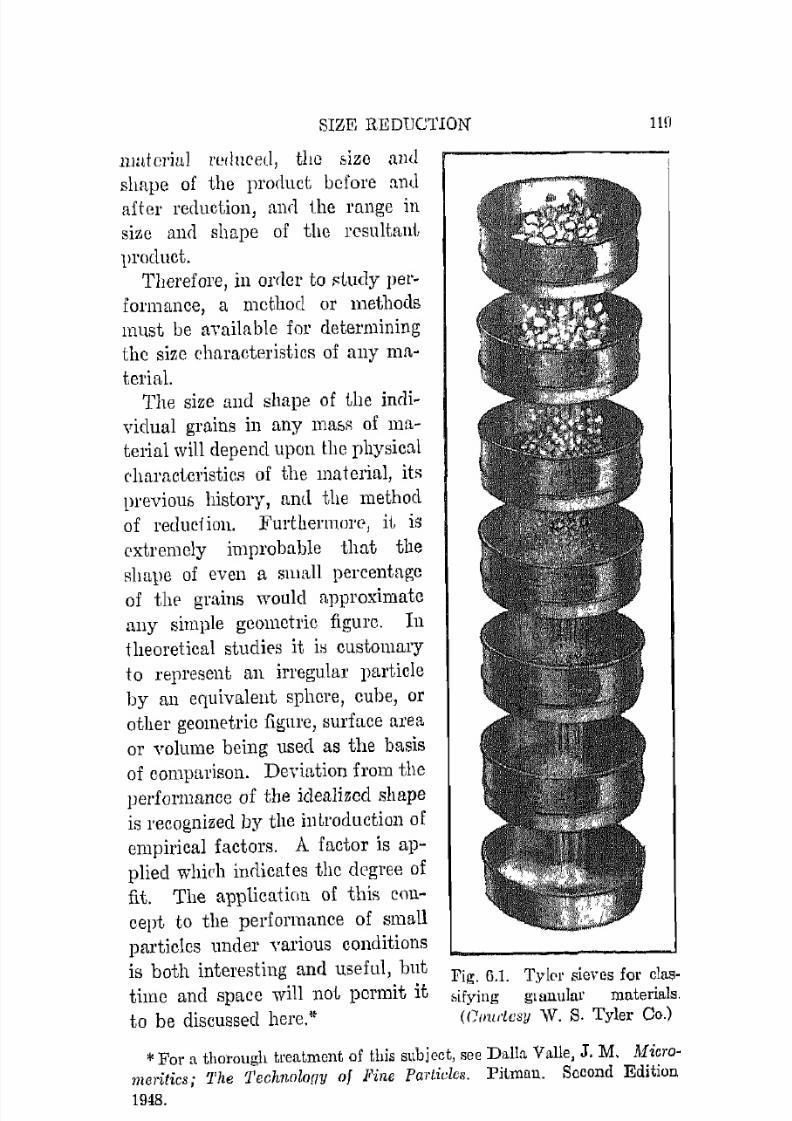
7/16/2019 Engenering Agriculture Perry
http://slidepdf.com/reader/full/engenering-agriculture-perry 128/422
SIZE REDUCTION
lllHtcriul reduced, the size and
Ilfl
shape of the product before and
after reduction, anrI the runge in
size and shape of the resultanj,
product.
Therefore, in oreler to :-;tudy per
formance, a method or methods
must be available for determining
the size characteristics of any ma
terial.The size and shape of the jncli
vidual grains in any maSR of ma
terial will depend upon the physical
eharactcristics of the material, its
previour, history, and the method
of reduci iOll. FurthennOl"c, it is
C'xtremely improbable that the
Rhnpe of even a small percentage
of the grains would approximate
any simple geometric figure. In
theoretical studies it iH customary
to represent an irregular particle
by an equivalent sphere, cube, or
other geometric figure, surface area
or volume being used as the basis
of comparison. Deviation from the
performance of the idealized shape
is recognized by the illLroduction of
empirical factors. A factor is ap
plied which inrlicates the degree of
fit. The application of this COll
cept to the performance of small
particles under yarious conditions
is both interesting and useful, but
time and space will not permit it
to be discussed here.*
Fig. 6.1. Tyler sieves for clas"ifying glunular materials.(CIlllJ"lcsy W. S. Tyler Co.)
*For a thorough tl'eatmcnt of this subject, see Dalh Valle, J. M. Micrornc)'itics i 'J'he Technology of Pine Partidcs. Pitman. Second Edition
1948.
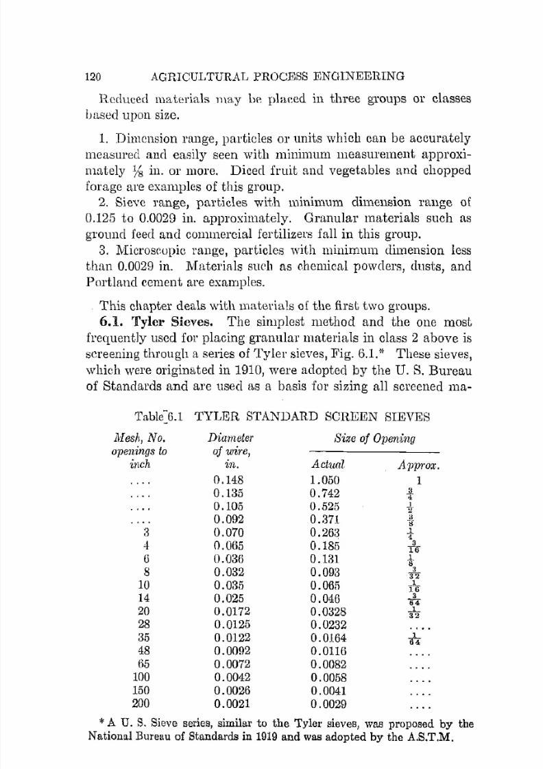
7/16/2019 Engenering Agriculture Perry
http://slidepdf.com/reader/full/engenering-agriculture-perry 129/422
120 AGRICUI,TURAL PROCESS ENGINEERING
R.cdueed materials may bp placed in three groups or classes
based upon size.
1. Dimcnsion range, particles or units which can be accurately
measured and easily seen with millilllum measurement approxi
mately % in. or more. Diced fruit and vegetables and chopped
foragc are examples of this group.2. Sieve range, particles with minimum dimension range of
0.125 to 0.0029 in. approximately. Granular materials such as
ground feed and cOlllmercial fertilizers fall in this group.3. Microscopic range, particles with minimum dimension less
than 0.0029 in. Materials such as ehcmical powders, dusts, andPortland cement are examples.
This chapter deals with materials of the flrst two groups.
6.1. Tyler Sieves. The simplest method and the one most
frequently used for placing granul::tl' materials in class 2 above is
screening through a series of Tyler sieves, Fig. 6.1.* These sieves,
which were originated in 1910, were adopted by the U. S. Bureau
of Standards and are used as a basis for sizing all screened 1113.-
'l'abl(6.1
l1Iesh, No,openings to
inch
a4o8
1014202835
48115100150200
TYLER STANDARD SCREEN SIEVES
Diameter Size of Openingof wire,
in. Actual Approx.0.148 1.050 10.135 0.742 !0.105 0.525 1
Y
0.092 0.371a
"j,i
0.070 0.263 .14
0.005 0.185 316
O.03ti 0.181 1"8
0.032 0,093 332
0.035 0.065 l16
0.025 0.046 l40.0172 0.0328 l
32
0.0125 0.02320.0122 0.0164 1
64
0.0092 0.01160.0072 0,00820.0042 0,00580,0026 0.00410.0021 0.0029
*AU. S. Sieve series, similar to the Tyler sieves, was proposed by theNational Bureau of Standards in 1919 and was adopted by the A.S.T.M,

7/16/2019 Engenering Agriculture Perry
http://slidepdf.com/reader/full/engenering-agriculture-perry 130/422
SIZE REDUCTION 121
terials used in processing Theil' characteristics are given in
Table 6.1.
The sieves listed in Table 6.1 constitute a normal set. Theopening size is bar:,ed upon the 200-11wsh t-ieve, eaf')l openillg lw
ing V2 or 1.414 times [ lb largc as the previolls um'. The oprnings
are squarc, the size heing thc dimen"inn of ow' :--ide. Intel'-
FIg. 62. A Ro-Tap machine used for a flieve unalysis requiring prerib€I'f'sults. (Conrtesy W. S. Tyler Co.)
mediate sieves wIth opening ratios of y2 or 1.189 are available
and, if added, would constitute a complete set. Note that if every
other screen is omitted 1I l the normal set that each opening will
be twice the previous one. This is tin important feature as regards
many size-reduction studies.
The techniques used in screening a sample l1(we been standardized and should be followed if significant results are to be
expected. The method and time of shaking are both important;
recommended procedures should be consulted and followed when
precise, significant data are required. A shaking machine, called
a Ro-Tap, Fig. 6.2, which has a definite shaking motion and can
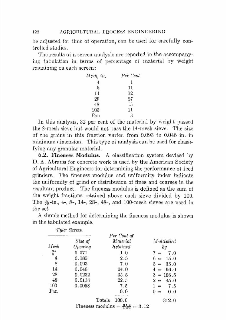
7/16/2019 Engenering Agriculture Perry
http://slidepdf.com/reader/full/engenering-agriculture-perry 131/422
122 AGRICTTLTtJRAL PROCESS ENGINEERING
be adjuEitecl for tjme of operation, can be used for carefully con
trolled studies.
The res\llts of n screen analysis are reported in the accompanying tabulation in terms of percentage of material by weight
r e m ~ t i n i l l g on each screen:
Mcsh, i l l . Per ('ent
4 18 11
14
21' 2748 ]5
100 11Pnn a
In this analysis, 32 pel' cent of the material by weight passed
thc 8-111es11 sieve but would not pass the 14-1118sh sieve. The size
of the grains in this fraction varied from 0.093 to O.04fj in. in
minimum rlimension. This typc of analysis can be used for clas::;i
Tying any granular material.
6.2. Fineness Modulus. A classification system devised by
D. A. Abrams for concrete work is used by the American Societyof Agricultural Engineers for determining the performance of feed
grinders. The fineness modulus and uniformity index indicate
the uniformity of grind or distribution of fines and coarses in the
resultant product. The finencss modulus is defined as the sum of
the weight fractions retained above each sieve divided by 100.
The %-in., 4-, 8-, 1 4 ~ , 28-, 4 8 ~ , and lOa-mesh sieves are llsed in
the set.
A simple method for determining the fineness modulus is shownin the tabulated example.
Tuler ScreenPer Cent of
Size oj Material MnltipliedMesh Opening Retm:ned by
!J!!lU71 1.0 7 = 7.0f
4 0.185 2.5 ()= 15.08 0.0!):1 7.0 5= 35.0
14 0.046 24.0 4= 9().028 0.0232 35.5 :3 = 106.548 O.OIHi 22.5 2= 45.0
100 0.0058 7.5 1 = 7.5Pan 0.0 0= O.D
Totals 100.0 312.0Fineness modulus = tPo = 3. 12

7/16/2019 Engenering Agriculture Perry
http://slidepdf.com/reader/full/engenering-agriculture-perry 132/422
SIZE REDUC'rIOK
The stallllani pl'oeedure spec·iiic;.; lL 2iiU-g ;'i:llnple oven dried to
constant weight at 212°], and Hhaken ill the lto-TalJ £(11' 5 mill.
Note that if all the material were fine onough to pa:3S throughall the screens inclwling No. ±S hut would hI:' retaine(] un No. IOU
the modulus would be 1.0. On the uthl'l' band, if aU1Hl'e rr'tailwd
on No.4 scrC'en, the modulus would be G.O.
The fwerage size of grain n in indies im[inlted by a lIlutiUiUH
nUllllll'r F.1VI. Cftll he f'aleulntp(l hy the following equation,
JJ = n.()O-!1(2)F..\L
which is shown graphically in Fig. n.:1.
0,6--t··_-
0,4.._--
I' - ~ l - -
0.21-;V
0.1
0,08
- - ~ - ~ ~- - ..
. ._ _.
,5 0.06 /
'" 0.04U5/ _---- ._
v
lZl..
- 4
--_ . -
0.02/ -
V--_
28
0.01/ - 48
0.008
0.006 /'/ 100
0.004V
200
0.002 a2 3 4 5 6 7
Fineness modulus
(l). 1,)
Fig. fi.a. Rp]lllionship bpt\vecn the fillt'nCSR Il1rHiulus and averuge ] l a l ' t i d , ~siZe. Ricvps are included io r refcrencp.
6.3. Uniformity Index. Although the fineness llloliulus gives
an avernge size, it does not indicate tho d i ~ t l ' i b u t i o n of the f i n e ~and coarses in any sample, and the average grain ::;ize is not pro
portional to the lt10Llulus index. These obj ection::l call be over
COllle by using the uniformity index which is demonstrated on

7/16/2019 Engenering Agriculture Perry
http://slidepdf.com/reader/full/engenering-agriculture-perry 133/422
124 AGRICULTURAL PROCESS ENGINEERING
the basis of the tabulated analysis. The ratio l : 6: 3 which must
totallO, determined as in the table, indicates the relative propor
tions of coarse, mediulll, and fine materials which are not inclicated by the fi.neness modulus, 3.12. The recommended proce
dure is to quote both indices, thus: 3.12,1:6:3.
BA Pel' Cent of
Screen iVlatcrial(Me.qh) Retained
:1 1.0"if
4 2.58 7.0
Total 10.5
1'1 24.028 35.1\
Total 5\).5
48 22.5
100 7.5Pall 0.0
Total 30.0
C'l'otals
Diliiderl by10
1.05
5.\)5
3.00
DCvlumn C
R 0 1 t 1 ~ d e d toNearest
Whole Number
Coarse
1
Medium
6
Fine
3
Note that only two screcns, numbers 8 and 28, would be re
quired to secure a uniformity index if the fineness modulus were
not required.
VaLue of G?'ound Feed. A great number of feeding tests of
various feeds have been made with the several types of livestockand poultry to determine the value of grinding feed. These tests
and accepted farm practice show that coarse grinding is advisablein most cases, specific over-all recommendations being as follows.
I t is not advisable under any condition to feed finely groundgrain to farm animals except small chicks, and for them theground grain granules should not be powdery. Tests show that
the fine material does not perform any better and in some cases
not as well as larger granules. I t is believed that the finelyground materials pass through the digestive tract too fast to beacted upon by the various digestive processes.
Grinding of forage is quest.ionable as regards its feeding value.Coarsely chopped hay and stover may be advisable to minimize
the amount of material thrown out of the feed bunks by the

7/16/2019 Engenering Agriculture Perry
http://slidepdf.com/reader/full/engenering-agriculture-perry 134/422
SIZE HE.DUC'TION 125
animals, but there it> little indieatiul1 that the feeding valnG is
increased. Chopping lIlay he justified in oreIcr to mix a less
palatable but nutritious forage with other feed. Fine (,hoppingor grinding doE's not. illlprove the fomgc and \\'ill )1l'Ollllbly lower
its quality by exp0f;urc to oxil[izutiull. Abo, tllU ahility of the
animBJ to dige\',t th.(', mt\tetial w\\1 \\(', \ ~ e \ ~ \ ' ~ " \ \ \ - l \ ~ ( l . AH\\If\1. \ \ l \ \ \
other forage crops fur poultry allil pig::; 11l11sL he !!;nJllwl fine to
provide consistency for eating.
The classification of ground grains amI forag\:s into eOarFl",
medium, and fine grades on the h a s i ~ of modulus illrlice" by
Silver 15 is given in Table 6.2.
Tahle 6.2 Ii'INENESS MODlTLtTt4 FUH ( , L A ~ ~ I F Y I P ; ( ;GHOUND FEEDS
GrindWhole ~ - - -
Material Clmin Coarse Medium Fine Fe1'Y FiliI'
Ear corn 4.80 a.GO 2 AO 1.80
i:lhellecl corn (LOO '1.80 a.GO 2.'10 l.SO
Barley 5.00 4.10 :1.20 2.;{0 1 . riOOat:;; <i.50 :3.70 2.0() 2.10 1.<10
MoybCltnS G.OO 4.80 :1. GO 2.-W 1. SO
Wheat 5.00 ·i.10 :1.20 2.aO UiOCOl'll fodder 5.50 -1-.20 2.00
Hay 4.00 :UO 2.20 t. 40
6.4·, Energy Requirements. C o m ~ i d c l ' the syltlmetrical par
tide in. Fig. 6A which is to he rCI.h1cccl to sym_mctti{"{I,l p ~ ' \ , l ' t i d ( , t \
of a smaller size. Figure 6.4could be represented as a
cube, a parallelepiped, a
sphere, or SOllle other shape.
The particles resulting from
the reduction could be any
shape or a great number of
shapes.
The required energy must
be related to SOlne function of
the initial and reduced parti
cle, and, since the particles
Fig. 6.4. An idealized particle which
is lobe reduced to geometrically sim
ilar particles.
are assumed symmetrical, a common dimension would probably
be used so that:
7/16/2019 Engenering Agriculture Perry
http://slidepdf.com/reader/full/engenering-agriculture-perry 135/422
126 AGRICULTURAL PROCESS ENGINEERING
t:.E 0: t:.L1jL'" (6.2)
ort:.E = G t:.LjL" (6.3)
This g c n e r a l i z f ~ t i o l l implies that the energy required to reduce aunit is proportional to a dimension of the reduced particle relative
to a similar dimension of the original particle raised to some
power n.Therefore, the energy necessary to reduce a specific mass of
particles from one size to another is:
fl1LdL
E = -c -L L"
(fjA)
Kick assumed that the energy requirements Hre a fUllction of a
common dimension of the material; so n = 1. in equation 6.3.
Therefore, the energy requirements arc:
E = GIn (LdI-z) (6.5)
Equation 6.5 is known as Kick's law.
Rittinger assumed that size reduction is essentially a shearing
procedure. Consequently, the energy required is proportional to
the llew surfaces createe!, which in turn are proportional to the
square of a commOll linear dimension. Therefore n in equation
6.4 equals 2 and the energy requirements are:
(6.6)
This equation is known as Rittinger's law.
Integrating equation 6.4 gives a generalized relationship,
(6.7)
For example, if 5 hp-hr are required to reduce a material from7:I:-in. size to 10 mesh, how much power would be required if thethe reduction were to 20 mesh?

7/16/2019 Engenering Agriculture Perry
http://slidepdf.com/reader/full/engenering-agriculture-perry 136/422
SIZE REDl7CTION
By Kick's law:
E = C In (LdL2)
5------ = 8.5GIn (0.25/0.(jli5)
:. E = 8.56 In (0.25/0.0328) = 7.55 hp-hr
By Hittinger's law:
E=C(2_-2_)L2 Ll
Ec=------
5- = 0.438
(I/O.OG5) - (1/0.25)
:. E = OA38(1/0.0328) - (1/0.25) = 1Ul hp-hr
12,
Kick's and Rittinger's la.ws were developed from stmlieti of
materials common to the chemical and meclumical ('llgineering
areas, talc, coal, limestone, etc., being examples. Such materialsare different from agricultuml materials snch as forage, slllall
grains, and fertilizer components. Considerable deviation from
these laws may be eX]lected when studying reduction of such
agricultural materials.
SIZE-REDUCTION PROCEDURES
The size of agricultural products is reduced by (1) rutting,(2) crushing, and (3) shearing either singly or in combination.
6.5. Cutting is separation or reduction which ii:l produced by
pushing or forcing a thin, sharp knife through the material to
be reduced. 1Vlinimum deformation and rupture of the reduecd
particles results. The new surfaces that are produced by the
sharp edge of the knife are relatively nndamaged. Cutting is
especially well adapted for reduction of fruit tlncl vcgetnbles_
Since the pores in the new surfaces are open because of minimum
damage from the sharp edge, drying or leaching or any process
requiring transfer of a liquid or vapor to or from the matcrial
proceeds at a maximum rnte.
The most satisfactory cutting device is a knife of extreme
sharpness and as thin as structurally possible. The motion of the

7/16/2019 Engenering Agriculture Perry
http://slidepdf.com/reader/full/engenering-agriculture-perry 137/422
128 AGRICULTURAL PROCESS ENGINEERING
knife should be such that the edge bas a sawing component inmoving through the material. This provides a smoother cut, prob
ably with less energy.6.6. Cl'Ushing is reduction by applying a force to the unit to
be reduced in excess of its strcngth. Failure results by ruptureof the material in many directions. The resulting particles are
irregular in shape and size. The characteristics of the new surfaces and particles are dependent upon the type of material and
the method of force application.
Limestone and other chemical fertilizers, ground feed for live
stock, flour and meal, and fruit. and vegetable purees are pro
duced in part or whole by crushing. Crushing is used to extract
juice from sugar cane and to break t.he structure of forage crops
to speed drying.
The force used in crushing can be applied statically as is done
when cracking a walnut in a vise or dynamically as with a
hammer. Crushing by llleans of a rigid roll or bed such as the
sorghum mill is au example of static force application. The
hammer mill exemplifies dynamic force application.
6.7. Shearing is a combination of cutting and crllShing. I fI!I>
the shearing edge is thin and sharp, performance approaches that
of cutting. A thick, dull shearing edge performs more as a
crusher.
Shearing is usually used for reducing materials of a tough
fibrous nature where some crushing Illay be advantageous and
the resulting units arc of large uniform size. Cutting ensilage is
an example.
The shearing units consist of a sharp knife and a bar. The
knife is usually thick to withstand the shock that results when
it hits the material. For best performance, the clearance between
the bar and the knife should be as small as possible and the knife
as sharp and thin as practicable.
REDUCING DEVICES
6.8a. Hammer Mills. The hammer mill is used for a variety
of size-reduction or "grinding" jobs. Besides feed preparation, it
is used for pulverizing limestone and the ingredients for commer
cial fertilizers. I t also has many industrial applications.

7/16/2019 Engenering Agriculture Perry
http://slidepdf.com/reader/full/engenering-agriculture-perry 138/422
SIZE REDUCTION
A hammer mill ('omi.,ts p ~ s e I 1 t i l l l l y of H lObtmg heatf'l' nnd 11
heavy perforated screen, F1!-b G.'). The materIal i" mlroducrd
mto the housmg, and thc beatcl', winch r n n ~ i ~ t ~ Ilf a serlc:" ufhammers turning at 1500 to -WOO rpm, heah amI pOllnd., the
Flg 65 Phantom vIew of a h,lmnH'l 111lIl Wlth II ( 'y! lone for colll!rtmg the
]uiu('cd m.ltpllai (Co!l1lc'Y John DueJe Co.)
material until it is small enough to pas" through the screen at
the bottom. Finelle"" uf division if> controlled mainly by the size
of holes in the :;,creen, although the rotor revolutions per minute
and the rate of feed are additional control factors.The hammers are rigidly fixed to the shaft or swing as shown
in Fig. 65. There is less clrmger of the "winging hammer causing
damage if a lalge metallic object gets into the mill by accident.
The striking edge of the hammer is designed in a great many
ways, thus indicating that there is no one be&t design. The
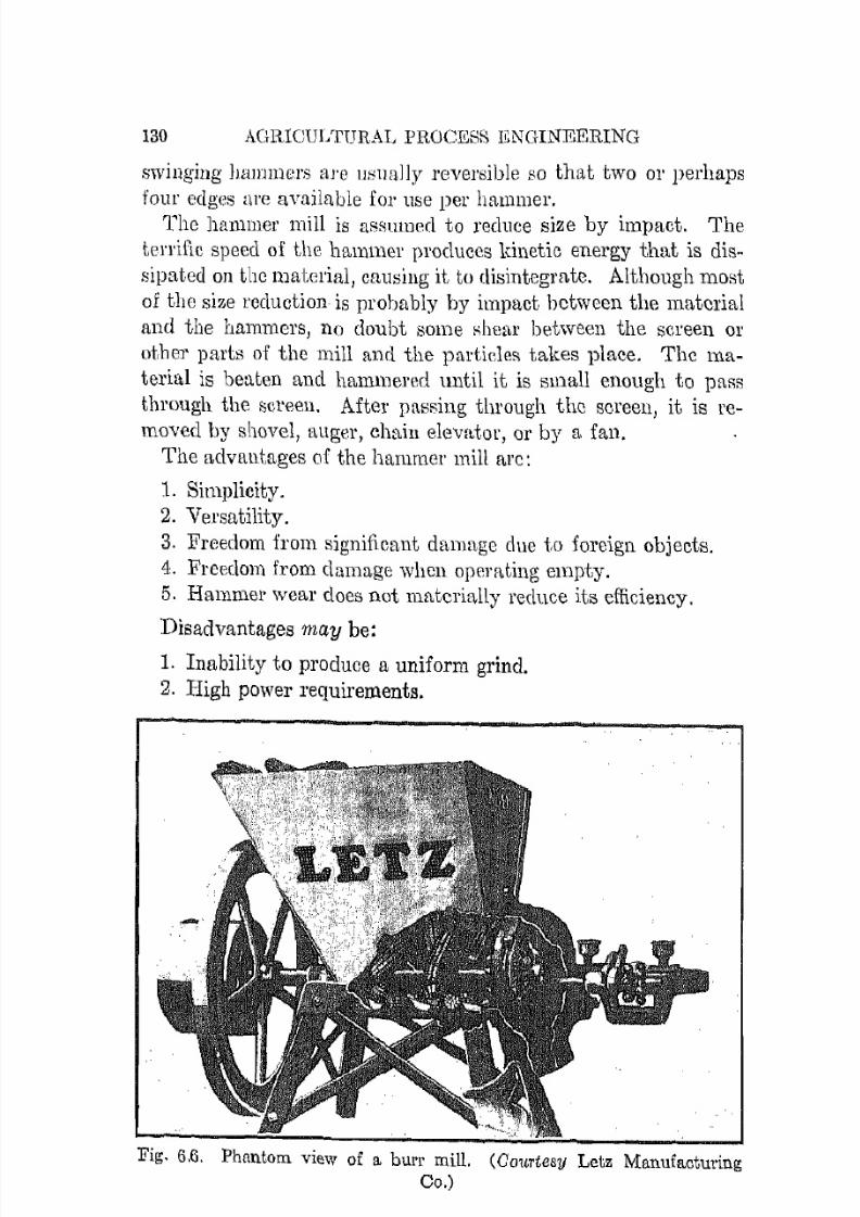
7/16/2019 Engenering Agriculture Perry
http://slidepdf.com/reader/full/engenering-agriculture-perry 139/422
130 AGRICULTURAL PROCgSS ENGINEERING
swinging lJaJrlmcrs a n ~ lL'iually reversible so that two 01' perhaps
four edges nrc tl,Yftilable for lise pel' hammer.
The hammer mill is ass\llned to reduce size by impact. The
terrific speed of the hammer produces l(illetic energy that is dis
sipated on the material, causing it to disintegrate. Although most
of the size reduction is probably by impact between the mf\torial
and the hammers, no doubt some shear between the screen 01'
other parts of the mill and the partielm\ takes place. The ma
terial is beaten and hammered until it is small enough to paSR
through the screen. After passing through the screen, it is re
moved by shovel, auger, chain elevlLtol', or by a fan.
The advantages of the hammer mill arc:
1. Simplicity.
2. Versatility.
3. Freedom from significant damage clue to foreign objects.4. Freedom from damage when opc]'[t(,ing empty.
5. Hammel' weal' does not materially reduce its efficiency.
Disadvantages may be:1. Inability to produce a uniform grind.
2. High power requirements.
Fig. 6.6. Phantom view of a burr mill. (Courtesy Letz Manufacturing00.)

7/16/2019 Engenering Agriculture Perry
http://slidepdf.com/reader/full/engenering-agriculture-perry 140/422
SIZE REDUCTION 131
6.8b. Bul'l' Mills. Burr mil!:;, also called plate lllilb, c O l l ~ i s tessentially of two l'ollghenecl plates, one statiunary, the 01 her l 'U
tating, Fig. G.B. The llHtit:l'i::tl is fed between tlJC plates U1Hl is
reduced by erushing and shear. I f the ll1atprial is fed slowly so
the fiuteR arc not fi.l1ecl, reductioJl is prohahly mainly by ;;hear.
With faster feed amI fiutps filled, hath :;,hear and e r l l ~ h i n g 110
No. A-233: Medium fine for small gruins, ear com.No. A-434: Medium fine for ~ l I l u l l grains, ear COl'll, roughage, high capacity.
No. B-41: Uniform conroe fol' small grains, ellr COl'll.
No. B-43: Extreme fine for dry small gmins, dry ear corn.
Fig. 6.7. Examples of "burrs" or "plates" for burr mills, a few of nHLuy
designs for various duties. (Coul'tesy L€'tz Manufacturing Co.)
doubt exist. Overfeeding reduces the effectivene;;s of the grinder,
and excessive heating results. The plates are d e ~ ; i g n e d for :1
variety of jobs (Fig. 6.7) and are usnally mude of chilled ca:;tiron although alloy steel may be advisable in certain case:,;.
Operating speeds are usually less than 1200 l·pm.
The fineness of reduetion is controlled by the type of plates
and by the spacing. The spacing screw is spring loaded so that
the space will increase in case of an overload or if a foreign object

7/16/2019 Engenering Agriculture Perry
http://slidepdf.com/reader/full/engenering-agriculture-perry 141/422
132 AGRICULTURAL PROCESS ENGINEERING
gets into the mill. Small rocks nIle! metallic objects may not
cause damage, but breakage can be expected i f large objects are
fed into the mill.The attrition mill is a heavy-duty precision "burr" mill used
in the commercial preparation of feed and food products. E!1ch
burr rotates and is driven independently, speeds arc much higher,
Hne! design and construction are morc precise.
The advantages of the burr mill are:
1. Low initial cost.
2. Product lllay be relatively uniform.3. Power requirements may be low.
Disadvantages are:
1. Foreign objects may cause breakage.2. Operating empty may cause excessive burl' wear.
8. INorn bUl'rs yield poor results.
6.9. Crushers. Crushers reduce the material by pressing or
squeezing it until the material breaks. Crushing is an importantindustrial operation, and a variety of types of machines are in
Fig. 6.8. Jaw and gyratory crushers. (Courtesy Allis-Chalmers Manufacturing Co.)

7/16/2019 Engenering Agriculture Perry
http://slidepdf.com/reader/full/engenering-agriculture-perry 142/422
SIZE REDurTION 133
Fig. 6.S. (contirlllrd).
use. Agricultural applicHtion of crusher::! is important out notextensive. The important adapLations will be rliscussed briefly.
Lime Etnd other stones arc given an initbl reduction by a jawor gyratory crusher, Fig. 6.8. The jaw crusher is the cheaper andthe slower of the two and is used for smaller operatiuns. The
shaft carrying the crushing cone in the gyratory crusher is free
turning. I t is loosely fitted at the top and is given a circulatorymotion of small amplitude at the bottom.
The resultant motion of the cone crushes the material in amanner similar to the jaw crusher, but operation is smoother andthe relative capacity is higher.
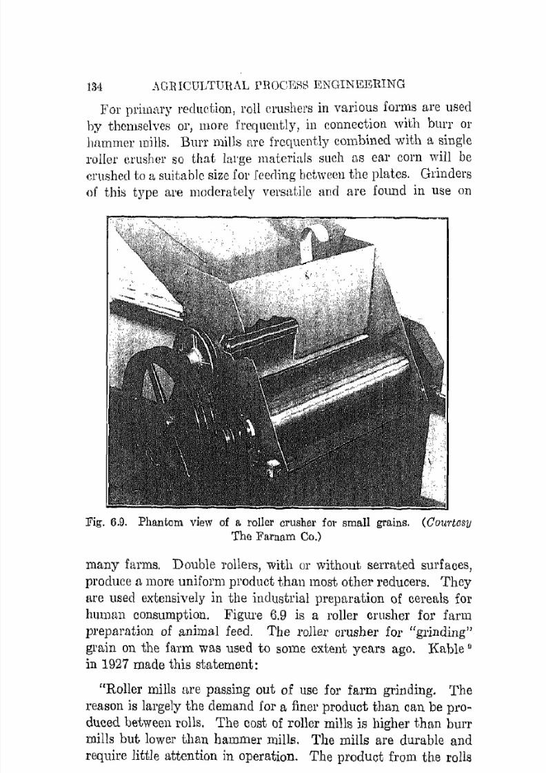
7/16/2019 Engenering Agriculture Perry
http://slidepdf.com/reader/full/engenering-agriculture-perry 143/422
134 AGRICULTUHAL PROCERS ENGINEERING
For primary reduction, roll crushers in various forms arc used
by themselves or, more frequently, in connection with burr 01'
hammer mjlls. Burr mills nre frcquently combined with a single
roller crusher so that large materials such [IS ear corn will becrushed to a suitablc size for Ieerling between the plates. Grinders
of this type are moderately versatile and arc found in use on
Fig. 6.9. Phantom view of a roller crusher for small grains. (Courtosy
The Farnam Co.)
many farms. Double rollers, with or without serrated surfaces,
produce a more uniform product than most other reducers. They
are used extensively in the industrial preparation of cereals forhuman consumption. Figure 6.9 is a roller crusher for farm
preparation of animal feed. The roller crusher for "grinding"grain on the farm was used to some extent years ago. l{able 9
in 1927 made this statement:
"Roller mills are passing out of use for farm grinding. Thereason is largely the demand for a finer product than can be pro"
duced between rolls. The cost of roller mills is higher than burr
ruills but lower than hammer mills. The mills are durable andrequire little attention in operation. The product from the rolls

7/16/2019 Engenering Agriculture Perry
http://slidepdf.com/reader/full/engenering-agriculture-perry 144/422
SIZE REDUCTION 135
in grinding barleYI wheat, and nol'll is not, dif'f'imilnr to that from
the burr mill exC'ept that the pcroeutage of fine mat orial obtnin
able is lower. Based upon the fcw tests mailr, tho pO\\'rr requiredfor rolling il:i somewhat greater than that W';cc! for the coarser
grinding with burr mills. The continued us(' of 1'\,11('1' mills will
depend largely upon whether the c o a r ~ e r grinding will !lwet farm
requirements."
I t is interesting to note that tlw major objcction tn roller milb
in 1927 is now a major asset in thaL the dcsirerl prorluet should
havefew fincs
and manycoarse particles. Th(' pOl'sibiliticK
()
ffarm nse of the roller crusher slll1ll1d be resun·cyed.
PERFORMANCE t:HARACTERISTICS
A size reducer opemting ideally would lmve tile following
charactcristics:
1. Product uniform as to size.
2. Minimum temperature rise during l'prlnction.:1. Minimum power requirement.
4. Trouble free operation.
Considerable investigational work has been done regarding tl1f'
performance of the varioul:i grindcl'R liKed in agl'ieulture, especially
burr and hammer mills. The performance of these deviccs will he
discussed in view of known applicable theory and test results.
6.10. Uniformity of Product. The burr mill is belicved to
produce a more uniform product thnn thc hammer mill. I f the
hammer mill reduces hy impact there are two factors Hmt could
contribute to this assumed undesirallle feature.
1. Anyone grain may be hit a nUlllber uf times before it has
an opportunity to pass through the scrcen. SincE' the path of
travel of a graiu through the grinder is random, the number of
times a grain is hit varies and as a reRnlt the size of the product
varies.2. The energy dissipated upon contact between a grain and a
hammer varies as the square of the velocity. Since the velocity
01' peripheral speed varies as the rotor radius, then the energy of
impact varies as the square of the l'adius1 or the energy of impact
at the end of a hammcr is four times as great as at a point hulf-

7/16/2019 Engenering Agriculture Perry
http://slidepdf.com/reader/full/engenering-agriculture-perry 145/422
136 AGRICULTURAL PROCESS ENGINEERING
way between the end of the hammer and the center of the shaft.
Consequently a grain that hits near the end of a hammer is more
Ilnely divided than one hitting closer to the shaft.
Now consider a number of grains passing between the burrs of
l), burr mill. Although shear is assullled to be the reduction
process, it is probable that most of the recluetiol1 is by crushing,
particularly if the rate of feed is high. Anyone grain is reduced
a number of times during the process, the number depending upon
the type of burrs being used and the random patll of the grain.
I f the material being ground is brittle and shatters upon fracture,it is possible that the resulting product will be made up of more
fine material than desired.
An average sieve analysis by Silver 15 taken from a number of
burl' and hammer mills of various types shows no significant dif
ference in uniformity between the mills.
The material in this case WHS of approximately 11 per ccnt
moisture content, which is moderately dry. "Vetter material
might perform in a different manner. ·With this exception thereported studies use modulus index us a measure of performance.
Sillce the modulus does not indicate the size distribution in the
sample, insufficient data are available to substantinte or refnt,e
this accepted pel'formance featme.
6.11. Power Requirements. 'rhe cxaet pow or required for a
specific job is difficult to determine. Type of material, moisture
content, fineness of grinding, rate of feed, type and condition of
mill, etc., affect the power requirements.
Some power observations by Silver 15 shown in Fig. 6.10 indi
cate that the more fibrous materials such as barley require more
power than a crystalline material such as corn.
Moist grains are mOre difficult to grind than dry grain. The
effect of moisture upon the power requirement is demonstrated
in Fig. 6.11 taken from Silver's investigation.
Test data for a hammer mill by Martin and Roberts 11 given in
Fig. 6.12 show the important characteristics of a hammer mill
using a fan for elevating the ground material.
The power required to operate the mill empty increases swiftly
as the speed increases since the power required to operate the
elevating fan varies as the cube of the speed (sect. 5.17). Con
sequently, eight times as much power would be required to operate

7/16/2019 Engenering Agriculture Perry
http://slidepdf.com/reader/full/engenering-agriculture-perry 146/422
SIZE REDUCTION 137
the fan at 4-100 rpm aH aL 2200. The eJllllty hOl'iiepUWer require
ment of a mill without a fall iii a. ~ t m i g h t - l i n e
function. Natethat the useful power, the differenec bctwet'I1 horsepower con
sumed ane! horsepower for running the mill empty, is a snwll per
centage of the input. Prom the standpoint of powrr C0118nmp-
30
25
20
~ar 15Ul
)5:c
10
5
I :7/j
/{'I IIV I IVN / { / /_vo ' l ; ~ I ".7 1 ' < 0
/ / !Jb/~ f i ? \ e o ,; "
....., r , Q ~ ( ! > "1--":"'.- ' b" \ " l ~ ,.- /
- - , "s'r-of!-,;-- Hammer mill",' .,,'" " . ... ",~ i ~ ( \ ~ oa\s", ' .. .,.. ---- Burr mill
.... _ .. "* -;:.",:: ... --
.J"::'" -----
4.0 3.6 3.2 2.8 2.4 2.0 1.6
Fineness modulus
Fig. 6.10. Relationship between power and fincnes5 of grinding for Llnecgrains liS ohserved by Sih·el'.lU Mills lire operatl'd at rajI'd speed. Gl'inrl
ing rule is 40 bu per hr. Coarse, medium, and fine b1ll'l's al'P u"f,d.
tion, operation below the rated flpeed is 11101'e advisable than
operatjon above.
Capacity in this ease is limited by the power available. III
order to maintain speeds above ,'3!iOO rpm, tlw feeding rate ha:i
to be reducecl so that a larger portion of the [lvailable power can
be UHcd for maintaining mill r;peccl.
6.12. Temperature Rise. The energy for grinding feed is
dissipated as heat energy and raises the temperature of the gl'ound
product., the mill, anu the ambient air. Some heat energy is lost
in vaporizing moisture.

7/16/2019 Engenering Agriculture Perry
http://slidepdf.com/reader/full/engenering-agriculture-perry 147/422
138 AGRICULTURAL PROCESS ENGINEERING
450
400
~ 350;:;;.
0 -;:;;.
~ ~ ~ ~ ~ /-fam
'"met '~ ~ 11ed~ I )~ 300
:B -......._ ~ ' ~ ---..::r---~ S q~ _I fI//eQ' c~ ~ t---
---carl) - . ; ;
I---. ~ , . , , 1 j-r------- r---eqr corn
.I!fco
;;0 250c:'5c:
;§ 200
150
10 12 14 16 18 20 22 24 26Moisture content, percent dry basis
Fig. 6.11. Effect of moisture content on capacity as observed by Silver.lf>
600
500
l : 400~
'"-n-_ 300z-'(3
'".'"u 200
100
V
V / '"
/ ~ v
-. . - Fineness
- J..---
2,4
:1>C}\'l --...,~ ~2,0/ ~ b
~1.6
V--! . ~ ~ <11( U l 1 ~ ::lI ' I ~ 4 :;-'00
1.2
0,8
EIII
'"~ - 0.4<llc:
i.i:
o 02800 3000 3200 3400 3600 3800 4000
Mill speed, rpm
L. ,
OJ5:00 .OJ<Il
:s:J:
I<'ig. 6.12. Performance of a hammer mill with a fan for removing the
ground material grinding shelled corn. (By Martin and Roberts.l l )

7/16/2019 Engenering Agriculture Perry
http://slidepdf.com/reader/full/engenering-agriculture-perry 148/422
SIZE DEDUCTION 13f)
Thc temperature may rj:;,c 50 0 P or more when p;rinding fibrous
materials such as oats or Pill' ('01'11 il l [ l butT mill, pnrtieubl'ly i f
a relatively fine grind is being prQ(hlf'ed. Tempcrature elenttions
of some materialR oh::;crvcd by ",ilYer 1:; are I'hown in Tahle 6.3.
Tahl!' ti.;{ MATERIAL TElIIPEHATnm Hl:->ED U R I N ( ~ CmmmN(l
1'P1I/11•
Tlfpr of F i l i e l l P 8 ~ Rlp/'( 1/ iOll,M([teri([l Orilllin J((/(Iullis OF
Oats Hurl' ~ . n flO
HUmIllel' 2.70 lS
Harley Bun :Ulfi 8HamIllrl' ;{ .1\(\ 2
Rhrlled ro!'ll Burl' on 7I-rammer :3. 1:1 10
Ear ('ol'n Bu)']' i:L07 14lIarnnwr a.on I" )
The hammer mill produces it cooler produrt because of the
large amount of ail' circulater! with the ground grain. High temperatures contribute to decomposition of the ground material l
especially if the moisture cont.ent is high.
MIXING
Mixing or blending of ingredients for animal feedR. fertilizers,
and seed stocks is an exten:-ive processing operation.
Difficulty in mixin!!; may result if the solhls arc the~ a m ( '
sizeand shape but of different speriflc gravity, or if they are of dif
ferent size ur shape. Heavier partir'les tend to remain nral' the
bottom of the container (luring a mixing operation. Round or
small partirles lend toward the top. ThiH tt'wlenry ('an be over
come by lifting the materials, mOl'e or l('::>H ill mass, frum the
bottom of the mixing cuntainer ami turning them onto Hnrl with
the top portion. A satisfaetul'Y mixing pl'(]epss (1) produces a
uniform mixture, (2) in H minimum time, (3) with a minimum
cost for overhead, power, and labor. A d i s c u s ~ i o n of the proce
dures follows.
6.13. Batch Mixers. Batch mixing is useel for moderate to
small operations where overhead costs must be low ancllabor costs
are not critica1. The ingredients may be weighed or measured.
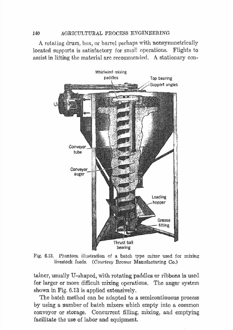
7/16/2019 Engenering Agriculture Perry
http://slidepdf.com/reader/full/engenering-agriculture-perry 149/422
1,10 AGRICUL'l'URAL PROCESS ENGINEERING
A rotating drum, box, or barrel perhapR ,yith nonsymmetrically
located supports is satisfactory for small operations. Flights to
assist in lifting the material arc recommenrled. A stationary con-
Whirlwind mixing
paddles
Fig. 6.13. Phantom i I l u ~ t r a t i o l l of a batch type mixer used for mixinglivestock feeds. (Cow·tesll Brower Manufacturing Co.)
tainer, usually U-shaped, with rota,ting paddles or ribbons is userl.
for larger or more difficult mixing operations. The auger system
shown in Fig. 6.13 is applied extensively.The batch method can be adapted to a semi continuous process
by using a number of batch mixers which empty into a common
conveyor or storage. Concurrent filling, mixing, and emptying
facilitate the use of labor and equipment.

7/16/2019 Engenering Agriculture Perry
http://slidepdf.com/reader/full/engenering-agriculture-perry 150/422
SIZE REDUCTION 141
6.14. Continuous Mixers. Continuous mixing procedures urc
most satisfactory for large, extensive operntions. The ingredients
are usually added volumetrically by [ I l l auger, star wheel, or otherdevice to a screw conveyor. I f more accurate control is requireri,automatic weighing machines Illay be used.
The continuous mixing operation is carried out in a screw con
veyor that may have special flights to insure a th()rough mixing
job. I f the blended product is conveyed some distance, no special
mixing unit may be required since the conveying opemtion will
mix satisfactorily.
6.15. Seed Treating. The application of fungicides and insecticides to control fungi and insects that attack I:)ccd before and
after planting is known as seed treating. The process consists of
mixing certain chemical!; with the seed. Sillce the rates of ap
plication are low, in the order of 7'2 to 2 OZ PCl' 100 lb, mixing
must be thorough to insure satisfactory result:>.
Mixing procedures are comparable to thosc tliscussed in the
previous sections. Since the quantities pl'oce::iscd are relatively
small when compared to feed-mixing opcrations, butch processesare usually used. Most of the dusts used are toxic, therefore
special health precautions must be observed.
REFERENCES
1. Alden, J. L. Design of Industrial E:!'haust Systems. The Industrial
Press. 1939.2. Bohstedt, G. Feed Processing in Rell1tion to Animal Nutrition. Aur.
Eng. 17 :98-100. 1936.3. Bruhn, H. D. Burr Mill Design and Performance. AgT. Eng. 17 :101-
lOG. 1936.4. Colby, H. N. Feed Grinding, Mixing, and Elevating. IVash. Agr. E;cpt.
Sta. Popular Bull. 151. 1937.5. Duffee, F. W. Testing the l ! J f I i l ~ i e n c y of Silage Cutters. Agr. Eng. 5 :3-6.
Jan., 1924.6. Duffee, F. W. Efficiently Filling the Silo. Agr. Eng. 6 :4-12. Jan., 1925.
7. Duffee, F. W. A Study of Factors Involved in Ensilrtge Cutter Design.
Agr. Eng. 7 :84-87. Mar., 1926.8. Fenton, F. C., and Logan, C. A. Farm Grinding of Grain and Forage.
Kans. Eng. Expt. Sta. Bull. 27. 1931.9. Kable, G. W. Results of Research in Feed Grinding. Agr. Eng. 8:53-54.
1927.10. Lapple, C. E., and Shepherd, C. B. ClLlculations of Particle Trajectories.
Ind. Eng. Chern. 32 :605-617. 1940.
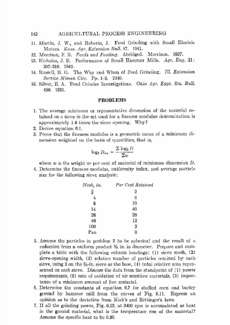
7/16/2019 Engenering Agriculture Perry
http://slidepdf.com/reader/full/engenering-agriculture-perry 151/422
142 AGlUCULTURAL PROCESS ENGINJDERING
1 L Martin, J. W., and Roberts, J. Feed Grinding with Smail Electrio
l\<1otor8. KUlls . .1(/)". Extension Bull,. 87. 1941.
12. Morrison, F. B. Feeds and Feedino. Abridged. Morrison. 1937.13. Nicholas, .T. E. Perfonn:mee of Smull Hammer Mills. Aar. Ena. 21:
20'1-210. 1940.
14. RllSsell, H. G. The Why and When of F ~ l e d Grinding. Ill. ExtenRion
Service Mimeo Cire. Pp. 1-5. 1940.15. Silver, E. A. Feed Grinder Investig11tions. Ohio Aor. Expt. Sta. Bull.
490. 1931.
PROBLEMS
1. The fl.veragc minimum or representative dimension of the material re
tained on a sieve in the set used for a fineness modulus determimttioll is
approximately 1.4 times the sieve opening. Why?
2. Derive equation 6.1.
3. Prove that the fineness modulus is a geometric meftn of 11 minimum di
mension weighted on the basis of C(uantities, that is,
Z log2Dlog2 D"v = - ~ - -~ w
where w is the weight or per cent of maLerial of minimulIl dimension D.
4. Determine the fineness modulus, uniformity index, allli average partich,size for the following sieve analysis:
ilfC8h, in.
1:l
4
8
14
2848
100Pan
Per Cent Retained
2(j
10
40
2812
2o
5. Assume the partic:les in problem 2 to be spherical llnd the reRldt of H
reduction from a tllliform product % in. in diameter. PreptLre and com
plete I t table with the following column headings: (1) sieve mesh, (2)
sieve-opening width, (3) relative number of particles retained by each
sieve, using 2 on the %-in. sieve as the bilSP., (4) total relative area repre
sented on each sieve. Discllss the data from the standpoint of (1) power
requirements, (2) rate of oxidation of air sensitive malerials, (3) impor
tance of a minimum amount of fine material.
6. Determine the constants of equation 6.7 for shelled corn and bl1rley
ground by hammer mill from the curves of Fig. 6.11. Express an
opinion as to the deviation from Kick's and Rittinger's laws.
7. I f all the grinding power, Fig. 6.12, at 3400 rpm is I1ccumubted as heat
in the ground material, what is the temperature rise of the material ?
Assume the specific heat to be 0.30.

7/16/2019 Engenering Agriculture Perry
http://slidepdf.com/reader/full/engenering-agriculture-perry 152/422
CHAPT]l. ;R,..I
C l e a n i n ~ <Hut Slll'tinM
NO]\'[ENCLATUllE
. t = projPctecl [1l'{'1L of ImrticIP, bq ft.
( ! = lL('celcrlLtional forc'p, ft pf'r SlW2,
b = entry width, ft.
C = particle aprorlynamic-drag ('opffirh'nt, ( l i l l H ' I J t ; , i " n l l ' ~ ' .{'J = cl'utrifugaJ foree, lb.
/) = uvemge partido diam('ter, ft.rl = diameter, ft.
tl' = JllLrticle diameter, in.E = e:-.it dunt diameter, rt.
F' = force, lb.g = acceleration of gravity, 32.2 ft lJl'r s ( ' c ' ~ .II = cone hcigh1" ft.
h = f'll try IWight, H.i ( = vane c o n ~ t a l l t , d i I l l e n H i o n l f ' ~ R .It = 11 ( ' O l l ~ t a n t , d i m c n ~ i o n l f ' ~ s .L = length, ft.
11;[ = particle r n a ~ s , Ih per Rec2 J)(,I' ft,.
N = number of turns.
n = revolutions per minute.
P = pressure drop, number of v<']neity heackR = mdius of l'otation, ft.
Re = lleYllolds number.
r = radius, ft .S = separating coufIiciunt, d i r n e n R i ( ) n k ~ s .V = relative velocity, ft per sec'.
vp = particle volllme, Cll fl.W = particle weight, lb.
l ' = fluid RplJcific weight, lb p01' ('U ft.1'p = particle ~ p e c i ! i c weight, Ib pel' eu ft .
J.lo = viscosity, 1b per ft-scc.() = tilllP, sec,
The comparath e commercial value of a farm produrt is a func
tion of its grade factor. Gl'ftcle factors have Leen establishcd by
various agencies interested in particular products and are recog-
143

7/16/2019 Engenering Agriculture Perry
http://slidepdf.com/reader/full/engenering-agriculture-perry 153/422
H4 AGRICULTURAL PROCESS ENGINEERING
nized by these agencies as the legal standard for cOlllmercial use.
Meat, dairy procluets, fruits, vegetables, forage crops, fiber crops,
grains, tobacco, etc., and their products are graded on the basis
of standards that are available, in general, from the Office of
Marketing Services, U. S. Department of Agriculture, Washing
ton, D. O.7.1. Gl'ade Facto!"s. Grade factors that apply in various com
binations to all tbe products produced 011 the farlll could be
classified thus:
1. Physical characteristics.a. Moisture content.
b. Unit size.
c. Unit weight.
d. Texture.
e. 00101'.
f. Foreign matter.
g. Shape.
2. Chemical characteristics.a. Analysis (composition).
b. Rancidit.y, free fatty aeid index (for fat-containing ma
terial) .
c. Odor and flavor.
3. Biological.
a. Germination.
b. Type and amount of insect damage.
c. Type and amount of mold damage.d. Bacteria count.
A processing aim is to handle and manipulate products so
that they will yield the highest possible net return after being
processed, initial quality of the raw products being recognized asthe important prime consideration.
General procedures that may be used to improve, maintain,
01' change the quality of a product are:
1. Control storage conditions which are:
a. Temperature.
b. Relative humidity.
c. Time.

7/16/2019 Engenering Agriculture Perry
http://slidepdf.com/reader/full/engenering-agriculture-perry 154/422
CLEANING AND SORTING 1<15
2. Kill or inhibit debtructive organi:;ulS by:
a. Fumigation.
b. Refrigeration.c. Heating.
3. Improve the physical characteristics by:
a. Changing or maintaining the moisture content.
b. Removal of foreign or dissimilar material.
c. Sorting into various fractions.
The procedures listed above have or will be treated directly 01'
indirectly in the chapters 011 air-vapor mixil1l'es, refrigeration,
and drying except 36 and c, removal of fureign or dissimillu' ma
terial and sorting into various fraetions wbich would be clean
ing and sorting and would apply to preparation of a material
for processing as well as grading of [1 commercial produ(·t.
Cleaning refers to the removal of foreign or dissimibr material.
This may be done by washing, screening, hand picking, or by
other means which are described later in this chapter.
Sorting refers to the separatiun of the clean8cl product into
various quality fractions that may be defined on the basis of size,shape, density, texture, and color. A di:;tinetion nhoulcl be noted
between sorting and grading. Grading implies the ciasi-Jification
of the material on the basis of cotn1l1rl'cial value unrl usngl) and
is dependent upon more factors than are recognized when physical
sOlting is considered. For exftmple, :;mall grain and certaiu fruits
and vegetables may be passed through a mechanical "gradel'''
which sorts the material on the ba:"is of size, "happ, or clcn::lity.
The mechanical "grader" is not effrctive as l'egurds mobtul'P content of the material, the amount of fungal or insect damage, or
germination. Conf'equently, the resulting fractiom; are not grades
as usually l'ecognized. On the other hand, if the matel'iu.l had
previously been sorted on the basis of moistUl'c content, damagC',
etc., the fractions produced merlumically might haye \)c('1) COlll
mercial grades.
The unit operations used in cleaning and Forting cannot Le
listed exclusively under either of these heads since some operations apply to both. For example, an air blast can be u:oed for
cleaning chaff from grain or for removing light weight seeus from
seed stock. A sieve can be used for cleaning sticks and leaves
from grain or for sorting out small, immature grain. The unit-

7/16/2019 Engenering Agriculture Perry
http://slidepdf.com/reader/full/engenering-agriculture-perry 155/422
146 AGlUCULTURAL PltOCESS ENGINEERING
opemtion discLUlsion that follows does not recognize the clenning
unci sorting classification as such.
WASHING
Fruits, vegetables, and nuts are sometimes washed to remove
dirt) Rpnty residues, and other foreign material. A prel iminary
cleaning operation by rongh screening may be used in certain
instanees; but the prodnct may be bruised, and therefore usual
practice is to place the product as delivered directly into the
washer.Washers may he eoutiullOllS or batch type. The batch type of
wasller is recommenderl only for smnll plants 01' institutional or
community installations where use is intermittent and operating
costs are not critical. ~ V n s h i n g is performed by one or a combina
tion of the following:
1. Sonking in still or moving water 01' other fluids.
2. Water sprays.
3. Rotary drum.
4. BotEl,Ling brushes.
5. Shuffle or shaker washers.
7.2. Soaking. Soaking in still or moving water 01' other fluids
is effective only if dirt, or other surface undesirables, is present
in small quantities and is loosely attached to the produet. This
method is frequently usccl in connection with other methods as [l,
precleaner or soaker.7.3. Water Sprays. 'Vater sprays that vary from low-pres
sure wide-angle to very high-pressure directed jets are very ef
fective since they physically remove firmly attached pieces of
dry dirt and agitate the mass of product, particularly if it is
carried in a water bath. Sprays are suitable for 1110st products,
but the intensity and type of spray distribution 111nst be carefnlly
selected. I t is evident that a high-pressure concentrated spray
for cleaning potatoes would be destructive to celery or lettuce.Flood washing is done by a large quanti.ty of water moving at
a moderate to high speed over the product.
7.4. Rotary Drum. This washer is the most commonly used
commercial washing device because of simplicity, high capacity,
thorough cleaning, and a minimum of damage to the product. I t

7/16/2019 Engenering Agriculture Perry
http://slidepdf.com/reader/full/engenering-agriculture-perry 156/422
CLEANING A ~ D SORTINCT 147
may be used in a hHtlt of water 01' with ~ p ] ' ( l y n [ ) z z l ( ' ~ , 01' both.
A rutary-type washer is :shuwn in Fig. 7.1 The p e r f ( ) 1 ' 1 l l ~ 1 1 l ( ' C asbased upon dirt l'ell1oyal is clrpendent UPU]} the J'otntiyc ~ p ( ' e l l , thr
roughness or amount of corrugating on Lhe i n ~ i ( l c fiurfare, and till'
Fig. 7.1. A rotary w,tshel'. The
material to bo washed IS screwedthrough t11P rotating drum. Note
tho nozzl('s for the applic:ltion ofOw waier. (Collrtesy Food MIt-
chinel'Y Corp.)

7/16/2019 Engenering Agriculture Perry
http://slidepdf.com/reader/full/engenering-agriculture-perry 157/422
1<18 AGHICULTURAL PROCESS ENGINEERING
length of time the product is retained in the washer. Auxiliary
aids such as spray nozzles may be used to facilitate thc job. Thc
washing time is controlled by the pitch of the drum or by helicalretaining fences which "screw" the product through the drum.
7.5. Brush Wasbel's. Rotating brushes are frequently usedand are highly effectivc. They are particularly effective for
removing sandy or loamy soil and for removing spray residues.
Washing time is controlled by the relntive motion of the brusheswhich moves the product through a definite path and to some
extent by the flow of wash water j f the brushes are opernting in a
water bath. The brushes are made of fiber, rubber, sponge, orother material nnd may have to be replaced frequently. This
expense must be considered in evaluating this typc of washer.7.6. Shuffle 01' Shaker Washer". These washers employ a
vigorous reciprocating motion. Since thc action is reciprocating,the washcr must be ruggedly constructed and carefully main
t.ained to minimize intcrruptions resulting from mechanical failurc. Although this type of washer is more complicated mechani
cally and more expensive than some of the other types, it is tobe recommended for the more difficult cleaning jobs. Although
effective because of its vigorous action, it is obviously unsuitedfor products that are easily damaged.
A sorting screen is frcquently included in the unit so that dirt,pieces of leaves, stems, and product fragments are washed awayfrom the material.
The best washing procedure usually utilizes two 01' more of thc
washing devices described. Also, the washing procedure can
usually be integrated with the movement of the raw product intothe plant. For example, washing and elevating can be combined.
Water flowing in a baffled trough will soak and remove part ofthe dirt and at the same time move the product from one opera
tion to anothcr. Spray nozzles userl in connection with the otherwashing devices frequently improve the performance.
Spray residues are removed from fruit by washing with a detergent solution, with a 0.5 to 1.0 pel' cent hydrochloric acid solu
tion at 70°F, or both. Immersion in a vat for periods up to 3min 01' power-spray washing for smaller periods will remove the
average deposit. Heavy wax formations or heavy oil-spray residues may require higher water temperatures or alkaline washes.
However, since these may damage the fruit, it is recommendedthat they be used only in extreme cases.

7/16/2019 Engenering Agriculture Perry
http://slidepdf.com/reader/full/engenering-agriculture-perry 158/422
CLEANING AND SORTING 119
Chemicals are frequently incorporated in the wUbh water to
control fungus, insect, and baderia growth. The la\\':; of the
Federal Food and Drug Administration. lirnit thl:"l sterilants used.and their residual tolerance where the 1 1 l ' ( l d u c t ~ are irl"\'oh"cd in
interstate commerce. Most. states have comparahle lnw" pertaining to products that are floIr! wit.hin the state.
Fig. 7.2. A comhination washer showing, in order, two soaking OPPl'lltions,
a spray washing operation, water removal, and drying. The ~ o : l k l l l g b.1thmay contain sterilizing chemicals, a matmial for spray lel>idufl removal, ormay be compounded for other pmposes. The htst few nm, of brushes may
be used for waxing.
A commercial washer using I t number uf the proeedures it>
shown schematically in Fig. 7.2. The brushes 111:1y be used for
waxing when advisable.
SORTING FRUITS AND VEGETABLES
FruiLs and vegetables ~ L l ' e sorted on the basis of eolor, Jamugc,
and size. Most sorting on the basis of color allll damage is dOllemanually but the dectric eye has been used successfully in pi.lot
studies, and its futUre general application appears promising.
Most fruits and vegetables are subject to damage if handled
too vigorously. Since {\, (telicate contact with the material and
high capacity are necessary, some unique procedures htwe been
devised.7.7. Screens.;; Many fruits and spherical vegetables are
graded over vibrating screens made of copper, stainless steel, 01'other materials which do not react chemically with the products.
The unsized material passes onto a vibrating or rotating screen
that, is perforated to pass all but the largest material, which goes
*Note sect. 7.11 for 0. more complete <.iisellssion of screens as used on ~ l 1 l a l lgrain.
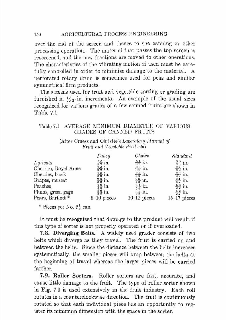
7/16/2019 Engenering Agriculture Perry
http://slidepdf.com/reader/full/engenering-agriculture-perry 159/422
150 AGRICULTURAL PROCESS ENGINEERING
over the end of the screen and thence to the canning or other
processing operation. The material that passes the top screen is
rc::;creened, and the new fractions are moved to other operations.The clwl'anLel'istics of the vibrEiting motion if used must be care
fully controlled in order to minimize damage to the material. A
perforated rotary drum is sometimes used for peas and similar
symmetrical firm products.
The screens used for fruit and vegetable sorting or grading are
furnished in 7 ~ 2 - i n . increments. An example of the usual sizes
recognized for various grades 0 [ a few eanued fruits are shown in
Tltble 7.1.
Table 7.1 AVERAGE MINIMUM DIAMETER OF VAmOUS
GRADES OF CANNED FR.UITS
(After Cruess nnc1 Christie's Laboratol'Y Jlilanual ofJll'llit and Vegetable Prodllc/H)
Apricots
Cherries, Royal AnneChenies, bhwk
Grapes, muscatPeaches
Fmw?/f iG 'a 2 111.
H in..2 0 ." j ! r 111.
-:}H- in.+ ~ i n .~ - ' 4 in.
Choicen 4, •1i"2111.
28 .::f!f Ill.
~ 4 i l l .I),) •
-3'2- lll .
· l ; ~ in.50 •a 2 111,
Standard
in.
" ! ~ ~ in.')r) •
·32 Ill.
~ 4 i n .- ~ L ! J in.
- ~ - ~ in.lums, green gagePears, Bartlett * 8-10 pieces 10-12 pieees 15-17 pieees
* Pieces per No. 2 ~ can.
I t must be recognized that damage to the product will result if
this type of sorter is not properly operated 01' if overloaded.7.8. Diverging Belts. A widely used grader consists of two
belts which diverge as they travel. The fruit is carried on and
between the belts, Since the distance between the helts increases
systematically, the smaller pieces will drop between the belts at
the beginning of travel whereas the larger pieces will be carried
farther.
7.9. Roller Sorters. Roller sorters are fast, accurate, and
cause little damage to the fruit. The type of roller sorter shown
in Fig. 7.3 is used extensively in the fruit industry. Each roll
rotates in a eounterclockwise direction. The fruit is continuously
rotated so that each individual pieee has an opportunity to reg
ister its minimum dimension with the space in the sorter.

7/16/2019 Engenering Agriculture Perry
http://slidepdf.com/reader/full/engenering-agriculture-perry 160/422
C'LEANIKG _\ND SORTli\G
T h i ~ roller KOlter is divided into three roll unite. "hieh al'p
hinged so thaL thc gaging t-Plll'C in(,1'('a;'('b ]ll'ugr('::o;:,ivcly tlil'Ollglt
the sorter. ~ \ y h e n the rolling unit d o ~ p " t h(' spare at the entl 01
its travel, tbe tllrning roller E'jceb without damage any frnit try
ing to pass through the space.
Roller conveyon, with fixpcl spare bri\,-rPlI the rolb an' Uf'et! forr('lDoving small fruit, twigH, a J l { l l e a y c ~ .
Fig. 73. A \,0]\(,1' ,mtl'\' rO l (Ott r \ l ~ (nut. ( C ( ) I ( l ' I ( ' . ~ I / Food l\1(ll'hinery Co)
7 .10. Weight Sorters. Rorter:> that operate Oll till' h a ~ i s ofunit weight ::\'1'e accurate i,nll lllodcratpjy fast and damage to the
material is miuimized. Weight :mrtcrll can he used on [til lal'gc
size products, apples, orangr:o;, calltcloupe, for example, and are
adapted to egg hnlHlling. Tlipy are especially useful for sortingmaterials that becau:;e of shupp or texture mC' not adapted toother pl'ocerlul'es.
The material is pla('cd into individual eU))H by nn automatic
indexing feed. As the f'Upi:l tran'l through the sorter they LLre in
dexed with spring-loaded trips. The spring tpn"ioll i" progres
sively weaker from bcginning to end of lllOVl'ment. TIll' heavier
units overcome thc spring reaetion and arc (lisrharg<,d at the
beginning uf travel, the lighter units moving a grcater <listance
before being discharged,
This sorting principle is not limited by size or shape of material.
The finencf1s of separation is deppmlent upon pr('('ision of design
and calibration aecu1'acy. I t will Jlot handle as large a quantity
of material per unit of time as other sorters.

7/16/2019 Engenering Agriculture Perry
http://slidepdf.com/reader/full/engenering-agriculture-perry 161/422
152 AGRICULTURAL l'lWCESS ENGINEERING
CLEANING AND SORTING GRAIN, NUTS, AND SEED
No distinct division can bc made between cleaning and sorting
of grain ancI various seed stocks since the process is carried onsimultaneously and the procedures are common to both.
Cleaning, sorting, and partial or perhaps final grading or classifying of the products being considered are based upon the follow
ing characteristics of the material:
1. Size.
2. Shape.3. Specific gravity.
4. Surface characteristics.
The first three are the most important. Surface characteristicsas differentiated from shape affect the drag coefficient where an
air blast is used for separation. Although it is known to be aneffective factor, its importance thus far has not been demon
strated. Roughness is used in ccrtain difficult cleaning operations,
which are discussed in sect. 7.16.7.11. Screens. The most widely used sorting device is the
screen or sieve. Screens used in conjunction with an air blaRt
will satisfactorily clean and sort, most granular products. The
screening unit is composed of two or more screens as shown inFig. 7.4. These screens are suspended by hangers in such a way
that they have a horizontal oscillating motion H and a smaller
vertical motion V, Fig. 7A.
The combination of these two motions moves the grain downthe screen and at the same time tosses it sufficiently so that the
sheet of grain is thoroughly stirred. The screen pitch is ad
justable. This. controls the rate of downward travel of the grain.
Screens are generally available with round, triangular or slotted
holes. Slotted screens may be punched sheet metal or wire cloth.
The slots may be orientated in the direction of travel, perpendicu
lar to it, 01' both.
Performance is based mainly upon careful selection of thescreens, although screen pitch is important. Generally speaking,
a relatively steep pitch does a better job. The material flows at
a faster rate and, consequently, is not so deep. On the other hand,
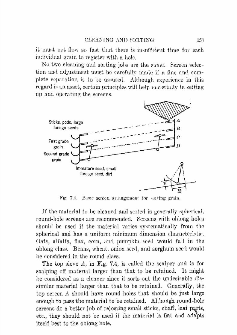
7/16/2019 Engenering Agriculture Perry
http://slidepdf.com/reader/full/engenering-agriculture-perry 162/422
CLEANING AND SOn:rrNO
it mu"t Hot flow SO fa..,t that tlwre is ill'\\lftlt'icllt time for each
individual grtlil1 to n ~ g i s t e r with a hole.Nu two cleaning and sorting job.., are the same. S e l ' e l ~ l 1 :;olee
tiOIl anll adjustment lllust be carefully malic if a fine and (,OlU
plete ~ e l l a m t i o n is to be ::I.8:-;1.11'el1. Although l'xperiC'lIce in this
regard if' an asset, certain principle,.; will help lHai erially in ,.;etting
up and operating the screenR.
Sticks, pods, largeforeign seeds
First grade
grain
Second grade
grain
----_-- _----
-_ ... - ..--
Immature seed, small
foreign seed, dirt
F))!: 7.4. B : t ~ l [ , screCll al'lttllgement for 'U) ting graill.
I f tho material to be cleaned and sartell is generally KJlhprical,
round-hole screenf1 are renoll1mcndl'd. Kcrecns with oblong 110](,8
i'lhoulcl be used if the material vltries sy:-;ternn.tically from the
spherical and has a uniform minimum dimenbion charal'tc'rif'tif'.Oats, alfalfa, flax, corn, ami pumpkin S('CI[ would fall in the
oblong clasR. Beans, wheat, onion seed, and sorghum seerl would
he considered in the ronnel olaf's.
'The top sieve A, in Fig. 7.4, is callE'd the scalper and is for
scalping off material larger than that to be retaincd. I t might
be considered as a cleaner sillce it sorts out the undesirable d i s ~similar material larger than that to be retained. Generally, the
top screen A shoulrl have round holes that should be just largeenough to pass the material to be retained. Although round-hole
screens do a better job of rej eding small sticks, chaff, leaf P\rts,
etc., they should not be used if the material is fiat and aclftpts
itself best to the oblong hole.

7/16/2019 Engenering Agriculture Perry
http://slidepdf.com/reader/full/engenering-agriculture-perry 163/422
lfi-l AGRIC[TLTURAL PROCESS BNGINEERING
rl'1w seeoml screon B should have holes just small enough to
retain the beRt material. I f the material is basically sphericaland the top fwreen ImH 1'0\.1l1d holes, the sceond screen B will prob
ably perform best if it, has slotted holes. COllversely, if the top
screen has slottccl holes, the 13 screen will probably perform best
with round holes.Frequently, screen C iN omHted, the light seccj and small ,veed
seed being permitted to fall onto the solid pan D. On the other
!tand if the lllaterial is to hc sOl't,ed into additional quality groups
Fig. 7.5. Efficient screen arrangement fat' most c ~ J e a n i n g and sorting jobs.
or if it is a mixture of materials that are to be sorted anc! re
tained, one or 1).10re additional screens may be required.
A more efficient screen arrangement is shown in Fig. 7.5. A
rough but accurate separation is made by the upper se!; of screens.The mixture that is to be Hortecl is freed of both large anel small
undesirable material and is concluded to the lower set of screens
where a finm' separation is mucIe, This arrangement is more
efficient than that shown in Fig. 7.4 sinee (1) the material is not
eontmnillatecl with the small fmetions rejected hy ]), (2) the
piteh uf the lower lmnk of sel'eens (',[\11 hc varied relative to the
upper bank, and (3) the vibrating ehal'acteristie can be varied
between the two sets to aecol1l11wdate the job at hand.When a fine degree of sorting is being mltde, grains will fre
quently lodge in the holes. Screens are frequently fitted with a
brush which travels under the screen and Ilushes the lodged ma
terial baek through the screen. There are other equally effective
devices.

7/16/2019 Engenering Agriculture Perry
http://slidepdf.com/reader/full/engenering-agriculture-perry 164/422
CLKI..NINn ANn RORTlxn 11).3
S(Jl'ecn cleaner,.; thaL Cillploy nn ail' b l a ~ t to a,,,,i,,t ill dCUllillg
are gcncrnlly knm\'Ila",
fauningmilk .A
"on v('ntional fnnning,mill of ihc type usclI by f,l'cd hOllE'''" j" ~ h m \ ' l l in Fig. 7.13.
Allbough they ('an lw and are llsed for jill ),.,t, ('lullIing and :-ort
ing work, tlwy are not, as tiplcdin' a;;; otll('1' r 1 1 · y i l · I ' . ~ in rcgard jn
, \ I
• \ I " - - - i ~ - - . . . _"' i,I,
I :::
Fig. 7.6. A (,Oll\'(;lltiona\ fmming mill showll in c r o , , ~ section. Tit" rough
Illlxime is ft'd froIll the lWlJper at the tOI). L a l ' g e - ~ i z e d fon·jllt! material
is taken off at 1. DUHL !lnd very light ~ p { · d s are aspimt ell at thC' hopper,
the light seed" nC[,1Illmiating at 2. The ilrsiraLle "r.ecl at:(JIlIll1llat l'S at ;1
and d i ~ { ' h a r g e s at. tllP bot tOIll, the Rlllallp,t "Of'" ar'('ull1ulatini!: al.·L Frac
tions bclw{;en 3 and the bottom di .dlfllW· al'f' cll']IUHite(! at Ii antI G. {( 'nl l l ' -
i1'811 A. T. Fen'pl! aw! Co.)
density. Also, if the seeds to be sorted have the 5ame or nearly
the same shape or Ilimcnsion, some other device is n e c e ~ : : , a r y .7.12. Aerodynamics of Small Particles. A particle in f1'l'('
fa.ll will reach a steady-state velocity that depends upon the
physical C'lunacteristics of the rarUrle, the fluid in which it isfalling, and the accelerational force. This partidc elmractcristic
is useful in pneumatic separation and ('onveying. The steudy
state velocity is also the air (or liquiJ) veloeity required to sus
pend or balance a prtrticle, thus the appJieahility to processing
opcl'ationfol.

7/16/2019 Engenering Agriculture Perry
http://slidepdf.com/reader/full/engenering-agriculture-perry 165/422
156 AGRICULTURAL PROCESS ENGINEERING
The following L),nalytical procedure is adapted from a treatment
of this particle characteristic by Lapple and Shepherd.n
F
The forces involved by a particle falling are
Jll(dT/jd8) = (vP'YJJ - v1J 'Y) - ]i'
.)[ 'Yp - 'Y 1"= .1. g-- - - I
'Yp
By definition
and equation 7.1 ean become
'Yp - 'Y V2'YAd V = ± g - ~ - - C - -'Yp 2gJJL
where A = projected area of particle, sq ft.
'Y = fluid specific weight, lb per Cll ft.
'Y1} = particle specific weight, lh per cu ft .
Vll ==: particle volume, cu H.
(7.1)
(7.2)
(7.3)
C ==: partide aerodynamic drag coefficient, dimensionless.
V = relative velocity, ft per sec.F = force, lb.
M = particle mass.W ==: particle weight, lb.
o= time, sec.
Be = Reynolds number.D = average particle diameter, ft.
The sign of the g (gravity) term is positive for a particle starting
from rest or having t tu initial downward velocity. The-sign isnegative for an initial upward velocity.

7/16/2019 Engenering Agriculture Perry
http://slidepdf.com/reader/full/engenering-agriculture-perry 166/422
CLE.\NI),'U AND :-:!URTIKG 157
I f I'P is larger than 'Y the particle motion will he dmnnmrd
,,{hen steady-state conditions haw heel} re!u'hed.I f the
fluid isclem;er than 1,he pltrtielc, 1,lmt it), ')' i;-; hnger than 11" the partir'll'
will rise during the stea(ly-statc condition.
For constant velocity, steady-state COll(litious, elF/da is Zpj"()
and equation 7.3 becumes
r = J i i 3 ~ ~ - : = ':;'(A Yp'Y
(7.
A direct solutioll of equation 7::1. is impnsHihlo sinee (J i:-; 11 funr'tirmof F. The velocity V ean hE' determined explicitly IJY the follow
ing procedure, however.
~"'"
""" Spheres --
DIscs - - - - -"- . ~
"- Cylinders ..........."- "~ ......', ...
".."-
... .' ~ ' ~ ,.-- ... .. ... --. _ -- ,..,-----......._ \
) - ~10'
Reynolds number. Re
Fig. 7.7. Drag coefficiGl1t as D. function of Reynolds )lumber (Table 7.2).The axis of the dise is parallel to t.he fluirl motion. The cylinder is of in
finite length; its axis is perpcndirlllm' to thl' fluid motion.
Studies with spheres, discs, and cylinders ha.ve shown a distinet
relationship between the drag coefficient C and Reynolds number,
Fig. 7.7. This relationship permits a solution in the followingmanner.
Re = DV'Y/fJ. (7.5)
and
V = Rep./D'Y (7.6)

7/16/2019 Engenering Agriculture Perry
http://slidepdf.com/reader/full/engenering-agriculture-perry 167/422
ViS AGRICULTURAL PROCBSS ENGINEERING
Eqnations 7A and 7.G are combined, and the following relatioll:-;hip
results.
eRe2 = 2gWD2
,,¥('Y1J - 1')p?A Y1J
(7.7)
Since thc right-hand terms of equation 7.7 are fixed by the system
beiug considcred, a value for CRe'J ( ~ a l l be determined.
Table 7.2 RELATIONRHIPS BETWEEN Re, 0, AND CRe2
.FOR SPHERES
Re C CRe2
0.12 ~ O
2.40.2 120 4.8
o.a 80 7.20.5 '19.5 12.40.7 36.5 17.91.0 2().5 26 ..52 14.4 57.68 10.4 98.75 0.9 1737 .5.4 2G5
10 4.1 41020 2.55 1.02 X ]Oa;30 2.00 1.8050 1 ..50 ;3. 7570 1.27 6.23
100 1.07 10.7200 0.77 ; ~ 0 . 8300 0.65 58.5500 0.55 138700 0.50 245
J.,OOO 0.46 4602,000 0.42 1.68 X 10⁶:3,000 0.40 3.605,000 0.385 9.607,000 0.390 19.1
10,000 0.405 40.520,000 0.45 18030,000 0.47 42(J50,000 0.49 1.23 X 10⁹
70,000 0.50 2.45
100,000 0.48 4.8200,000 0.42 16.8300,000 0.20 18.0400,000 0.084 13.4600,000 0.100 36.0
1,000,000 0.13 1303,000,000 0.20 1.8 X 10¹²

7/16/2019 Engenering Agriculture Perry
http://slidepdf.com/reader/full/engenering-agriculture-perry 168/422
CLr.A)lIN(; AND SORTING 1.W
.A plot 01' table u[ C ' R e ~ Y1:i. He -values pl'qltlreu from Fig. 7.7
for a specific-shaped pal'tide p e r l l 1 i t ~ the Ilcynoldti ll11111bel' ior
5tendy-statc conditiuns to he found. TulJlc 7.:! reports these rela
tionships for s p h e r e ~ . COlntmrable tables for (liKce! 01' cylilld('l's
could be prepared easily.
The Reynolds numher can be KllbHtituLu(l ill r(jllatirm 7.0, llnd
the steady-state velocity can he ealclllatell.
The velocity-time-distallce relatiullship for the elulllging -ve
locity period can be detrrlllinoci only lJY incremt'llt al solution of
equation 7.4.
Note t.hat this procedure t\pplil's for laminar, tnrbulenl" nnd
mixed flow. Turbulent flow exi:-;ts for Heynolds llumlJPrs g r e a t ( ~ rthan 500, laminar flow for thm;c less than 2, J,!1miuar mill turbu
lent flow may cxi::;t somewhat within the boundaries of Lhe :2 to
500 Reynolds 111llUUer bracket) hut this it:; generally l'L'cognizl)ll a,.,
the mixed-flow region.
7.13. Application. Agricultural p [ l l ' t i r l e ~ , outs, gnu.,;> sccLl,
ground lllaterials, dusts, sawdust, for example, do noc eonfonll to
any of the three geometric's di:-:cus$ed. Most particles du fallbetween Lwo of the gcollwtri(':-; or an approximate cquiYal('nt
Hphere can be assumed.
The geometric mean uf tile three axial, signifil'ant dimensiulls
is the diameter of :1n approxilllate eq\\iyalt,ltt tlpherc. This di
ameter should he used fur deterlllining the Pl'ojcctell area of tL
particle moving in the turbulent or ncar turbulent region. The
minimum cross-sectional area should be used for particleR moving;
in the laminar or near laminar region. Siew-size particles canbest be assumed spherical and of such a dimenHion ItS the sieve
analysis indicates.
7.14,. Pneumatic Separators. Fallning mills for farm use or
:,:mall seed-proces:-.;ing plant::; cOllsil:it es:;entially of a set of sc'reens
as described in Hect. 7.11 and a fan for moying air through the
graiu which removes chaff, tlirt, and ligbhveight seed. The sepa
rating effect of moving air is used by itself and iu connection with
other devices.The moving air for this method of denning and scparuting can
be provided by "blowing" througb the grain, lIll' air coming from
the discharge of a fan. Or it can be pl'oyided hy "drawing" the
air through the grain by (,(lllnectioll to the intake of a fan. The
latter process is called aspirating.

7/16/2019 Engenering Agriculture Perry
http://slidepdf.com/reader/full/engenering-agriculture-perry 169/422
lfiO AGRICULTURAL PROCESS ENGINEERING
The process set out in sect. 7.12 can be used for determining thepe1'£o1'111[lllce of pneumatic separators since the settling velocity Vis the factor upon which performance is based.I t is probable that the lighter fractions in wheat, for example,
and the heavier fractions in oats cannot be separated by thismethod. Consequently, pneumatic separators are usually used
with other cleaning procedures for separations that are not so
similar, or on material that has been precleaned or sized i f a
separation on a density basis is desired.This principle may also be used to separate falling grain by
altering the trajectory as it falls.7.15. Specific Gravity Sepa.rators. Gravity separators such
as shown in Fig. 7.8 are of recent adaptation and can make ac
curate separations under the more difficult sit.uations.
This separating device is based on t.wo conditions: (1) the
ability of a grain to flow down an inclined plane and (2) the
lifting or flottt.ing effect produced by the upward motion of air.
The lifting effect as shown in the previous section is a function
of size, shape, weight, and perhaps degree of surface roughness.
The prime unit of this separator is a triangular-shaped perfo
rated table. The table is so baffled underneath that air which
is fed up through it is evenly distributed. The volume of air,
which is supplied by a fan, is controllable within a wide range.
A plan and fl'Ont elevation of the table are shown in Fig. 7.8.
The table has a reciprocating motion that moves any material
upon it in the direction of conveyance. The table has vertical
adjustments such that it cnn be tipped toward the front and
toward the left, the net pitch being such that i t sphere placed
on the table would roll in the direction indicated by the angle-of
gravity-flow arrow. The pitch angles are shown in the discharge
edge elevation.
In operation, material is introduced into the feed box. Air is
blown up through the perforated floor at such a rate that the
material is partially lifted from contact with the floor. Lighter,smaller pieces are lifted somewhat higher and "float" down the
table toward the discharge edge. The large and heavy particles
are not lifted by the air. The oscillating motion of the table
moves them in the direction of conveyance, and they are dis
charged at the right edge of the table. Other material that is

7/16/2019 Engenering Agriculture Perry
http://slidepdf.com/reader/full/engenering-agriculture-perry 170/422
CLEANING AND SORTI)7G 161
only partially lifted touehcs the table frequpnt or infrequent
intervals and is discharged at an appropriate intermediate Jloinl.Hardware cloth, 1wrforated cOl'l'ugatcrlmetal, ct.mn!s, t!lHI other
floor coverings arc ::wailable to adapt the machine to val'ioll::o of
Top view of sepal at ing unit show
ing flow of matl'lltll J'rlativr to
angle of fl:1'l1Tity flow and direetion
of ('om'eyor
TrostJ Wt'evileilien
b e 3 n ~C ! e ~ n
b e i J n ~
Si,k view uf <eparatinu; unit show
ing mlltel'ial:l separation, angle of
inl'olllin::.': [IiI'. ane\ lilt of conveyor,
FIg. 7.8. Spel'ific gravity oep:uator. (COlO'tcsy Sutton. Steele, nnd Stt,ele
Co.)
a multitude of jobs. The discharge spouts can be varied as to
number and the discharge-cdge distance that each serves,
For rough work where the materials to be sorted are of diverse
size and weight the table pitch can be relatively steep, This
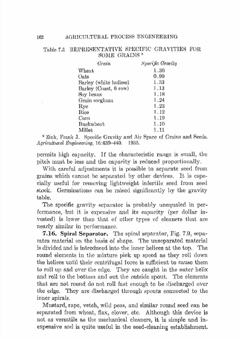
7/16/2019 Engenering Agriculture Perry
http://slidepdf.com/reader/full/engenering-agriculture-perry 171/422
162 AGRICUl,TURAL PROCESS ENGINEERING
Table 1.3 REPRESENTATIVE SPECIFIC GRAVITIES FORSOME GEArNS '"
WheatOats
Grain
Barley (white hullcss)Barley (Coast, (l row)Soy beansGrain ~ ( ) l ' g l l l l i l lRyeRice
CornBuekwhentMillet
Specific Gram:l:y
1.30
0.99
1.a31 .1.18
1.24
1.23
1.12
1.191.10
1.11*Zink, Frank J. Specific Gravity and AirSpace of Grains ami Seeds .
• ign:eultnral Engineering, 16:489-440. 1935.
permits high capacity. I f the characteristic range is Slllltll, thcpitch must be less and the capaeity is reduced proportionally.
With careful adjustments it is possible to separate seed from
grains which cannot be separated by other devices. I t is cspecially useful for removing lightweight infertile seed from seed
stock. Germinations (Jan be raised signifieantly by the gravity
table.
The specific gravity separator is probably unequaled in per
formance, but it is expensive and its capacity (per dollar invested) is lower than that of other types of cleaners that arc
nearly similar in pel'formance.
7.16. Spiral Separator. The spiral separator, Fig. 7.9, separates material on the basis of shape. The unscparated material
is divided and is introduced into the inner helices at the top. The
round elements in the mixture pick up speed as they roll clown
the helices until their eentrihlgal force is sufficient to cause them
to foHnp and over the edge. They are caught in the outer helix
and roll to the bottolll and out the outside spout. The elements
that are not rOllnd do not roll fast enough to be discharged over
the edge. They are discharged through spouts connected to theinner spirals.
Mustal'd, rapc, vetch, wild peas, and similar round seed can beseparated from wheat, flax, clover, etc. Although this device is
not as versatile as the mechanical cleaners, it is simple and in
expensive and is quite useful in the seed-cleaning establishment.
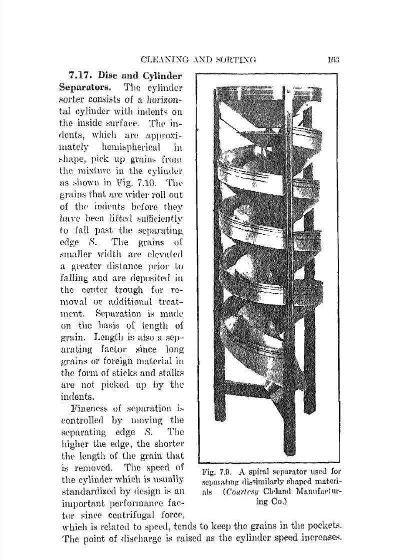
7/16/2019 Engenering Agriculture Perry
http://slidepdf.com/reader/full/engenering-agriculture-perry 172/422
C L K \ _ K I ~ G .\_XD SURTIX(l
7.17. Disc and Cylinder
Separators. The cylinder
sorter consistH of I), horizontal cylinder with indent" onthe inside Hurfarf'. The in
dents, whirll arc approxi
mately helllibphel'ieal ill
!-lmpe, pick up gmill!- frulll
the mixture in the cyliulicr
as "hown in Fig. 7.10. The
grains that are wieleI' roll out
of tIl!' indents lwfore they
have been lifted bu[ficicntly
to fall past the separating
edge 8. The grains of
:mmller width are elevah·d
a grpatel' di:-.tfmce )1riol' to
falling iLnd nre dellositpd ill
the center trough for removal or additional treat
llll'nt. Reparation is made
on the h a s i ~ of lengtll of
grain. Length is abo 11 sep
arating faetoI' Hinee long
grains or foreign material in
the forl11 of stirlcH and stalks
are not picked up by theindents.
Finen!:'sb of ~ e p a r a t i o n i"
controlled by nlOving the
RC'parnting edge 8. The
higher the edg(', the shorter
thp lcngth of the grain that
is removed. The speed of
the cylinder which is usuallystandardized by (ie:;ign i" an
important performanrc fae
tor l'ine(' centrifugai force,
Fig. 7.9. A spil'lll separator used for
SCjJHl ntmp; d i , ~ i m i l a l ' l y slJap('d materi[ l l ~ (Coul'trs/I Clpland Mallllfndnr-
ing Co.)
which is related to :;peed, tends to keep the grains in the p o c k e t ~ .The point of disdlarge is raised as the cyliJlder speed increases.

7/16/2019 Engenering Agriculture Perry
http://slidepdf.com/reader/full/engenering-agriculture-perry 173/422
164 AGRICULTURAL 1>iWCESS ENGINEERtNG
Fig. 7.10. Cross section aud plHllltom view of a cylinclm' sorter. (CourteBY
Hart-Carter Co.)

7/16/2019 Engenering Agriculture Perry
http://slidepdf.com/reader/full/engenering-agriculture-perry 174/422
OLEANINe; ANn SOHTI\;G loil
~'"';~;: "
'";:;;Co
2-
.;
~ .,-0
.8...!!S0>
.!<I<:J0p..
'":5.....0
p
.8 .-,"' 0
'" 0,
f2....E
0 ~.." U
"0
"Il
...0..-c:!
;;;~Ul
!)
't:I
c:!
.....0
r,:.s,;:-
S0
~[ ;
....;.....,.:
bO~

7/16/2019 Engenering Agriculture Perry
http://slidepdf.com/reader/full/engenering-agriculture-perry 175/422
166 Ac:mCULTURAL PROCESS ENGINEERING
TltiH sorting machine is especially useful for cleaning and sort
ing the graill into grade fl'l1ctions, particularly the sorting, wherelarge quantities of specific materials are handled. Milling and
seerl enterprises [tnd terminal grain elevators are examples. Even
though each machinc is fixcd as regards size of indents and speed
of operation, \Vide flexibility of use is possible. For example, It
Bingle lt1achine will handle cleaning llnd gi'ading operations per
taining to burley, whent, rye, ane! oats.
The disc separator of Fig. 7.11 separates on the basis of grain
length. The pockets, which are slightly undercut as shown in thefigure, can pick up and retain short grains, but long grains fall
(Jut. I t is especially adapted for removing dissimilar materials.
For example, wheat, rye, cockle, wild peas, mustard, wild buck
wheat, pigeon gmss, pin onts, and barley can be removed from
oatH. Similar sepnrations (Jan be made from other grains.
The mix to be sepam!;.ecl is moved through the machine oy
flights on the disc spokes. The material (which may be either
desirable or undesirablc) not lifted by the discs is tailed fromthe end of the separator. A number of distinct separations can
be made in a single machine by installing banks of rlises with
different characteristics. The pockets in the first bank of discs
are smaller than the second hank so that the smallest material is
removed first. The Beeond bank has larger pockets than the first,
and the next l n r g ~ r frac:tion is removed next. The largest grains
p a s ~ through the centOr of the elisC's and are tailed from the
machine.
Disc and cylinder separators have high captLcity. Since all
the moving parts are rotative rather than reciprocating, long life
and modera.te power requirements are eharacteristic. Each
machine is fitted with a cylinder or discs having fixed character
istics. Consequently, these separators are not as versatile as
certain other sorters. Even so, a single machine can be used for
it sufficient numher of separations to make it a general utility
machine for a milling or seed-processing cnterprise.
7.18. Separation Based upon Surface Texture. Surfacetexture may be used as u ba8is for separation when other methodsfail.
A principle shown in Fig. 7.12 is used to separate certain rough
'lYO€d seeds from useful seed of similar size, shape, and density.
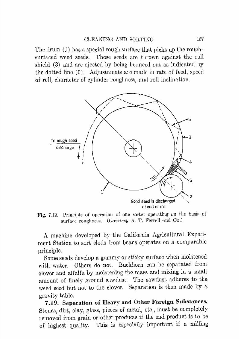
7/16/2019 Engenering Agriculture Perry
http://slidepdf.com/reader/full/engenering-agriculture-perry 176/422
CLEANINU ANn SORTING Hi7
The drum (1) has 11 special rough o11l'face that picks up Lhe roug,h
surfaced weed seeds. These spells are thrown agtlinst the rollshield (3) and are ejected by being bOllH('cd uut us indicate(l hy
the doti,ed line (G). Adjustments arc made ill rate of feed, speed
of roll, character of cylinder roughness, and roll inclination.
To rough seed
discharge
Good seed is discharged "at end of roll
6
3
4
5
2
Fig. 7.12. Principle of ojJPl'ation of one MorLer operlltiug un the busiR of
sUrfu('c roughness. (C01l1'tcsy A. T. Ferre1l1tnri Co.)
A machine developed by the California Agricultural Experiment Station to sort clods from beans operates on a comparable
principle.Some see(ls develop a gummy or sticky surface when moistened
with water. Others do not. Buckhorn can be separated from
clover and alfalfa by moistening the mass anLl mixing in a slUltll
amount of finely ground sawdust. The sawdusii adheres to the
w('cd seed bnt not to the clover. Separation is then Inade by a
gravity table.7.19. Separation of Heavy and Other Foreign Substances.
Stones, dirt, clay, glass, pieces of metal, etc., must be completely
removed from grain or other products if Lhe end product is to be
of highest quality. This is especially important i f a milling

7/16/2019 Engenering Agriculture Perry
http://slidepdf.com/reader/full/engenering-agriculture-perry 177/422
168 AGHICULTUHAL PROCESS ENGINEERING
process is to be used. Stones and metallic substances would be
destructive to milling machinery and would render the end product
unfit for human or, perhaps, animal consumption.Most of the heavy foreign materials will be removed during
the normal cleaning and sorting procedures, using one or more
of the devices discussed previously. However, certain special
procedures should be commented upon briefly.
A special gravity table comhined with air flotation operating
on the same principle as the gnwity table discussed in sect. 7.15
can separate all heavy foreign materials. I t has high capacity
and is especially useful for milling houses.Iron and steel pieces can be separated with magnetic separators.
Infrequently, hard clods are found in a product which are the
same size, shape, and density as the grains of the product. Con
sequently, they cannot be removed by any of the conventional
means.
Separation can usually be made by running the mixture be
tween two soft rubber rolls so spaced that the material is not
harmed but the clay pieces are sufficiently reduced in size to beremoved by screening, aspiration, or by some other mothod.
I f the clay pieces are too hard to be broken up by this method,
the special maehincs discussed in sect. 7.18 are usually s a t i s ~factory_
CENTRIFUGAL SEPARATION
The familiar farm cream separator separates the cream from
the skim milk by the centrifugal force resulting from rotation ofthe bowl. Industry uses this principle in many operations to
separate a suspended material, finely divided solid or liquid, from
a liquid-carrying medium. Although the cream separator is the
only familiar agricultural use for this type of separation, the
principles should be clearly understood so that application can be
made to any possible problem.
7.20. Stokes' Equation. Stokes' equation or law defines the
terminal or steady-state velocity of partioles moving under anaccelerational force with streamlined flow. Stokes' equation is
2r2(')'p -, -')')aV=-- - -
9f.t(7.8)

7/16/2019 Engenering Agriculture Perry
http://slidepdf.com/reader/full/engenering-agriculture-perry 178/422
CLEANING AND SORTING
where V = velocity, ft per sec.
r = radius of particle, ft.
/'1' = density of particle, lb per eu ft./' = density of fluid medium, lb per eu ft.a = tLCcelerational force, lb per sec2 • 1'
M = viscosity, lb pel" ft-::;ec.
169
I f the particle densiLy is greater than the density of the carry
ing medium, the particle will fall. I f less than the medium, the
particle will risco
The maximum or limiting radius for which Stokes' equationapplies is
(7.9)
As the particle size becomes smaller and approaches the size of
the molecules of the fluid mediulll, additional iaetors become ef
fective and SLakes' law does not apply. Homogenization oremulsification provides a physical bond that makes it difficult or
impossible to separate the su::;pended particles from the carrying
medium.
In the case of butter faL t:luspended in skim milk, the individual
particles of fat combine into clusters that have a larger effective
radius than the individual particles and, consequently, rise at a
faster rate. This phenomenon is characteristic of many emulsions
and suspensions, oils in water and gases in liquids, for example.7.21. The Centrifuge. Movement of dissimilar particles
through a fluid call be greatly speeded by increasing the accelera
tion factor a, by rotating the mixture or suspension about a fixed
axis. This fact is utilized in the centrifuge, which rotates a small
sample of the material around an axis at a high rate of speed.
Equipmcnt of this type is familiar to laboratory technicians.
The centrifuge used in determining the butter-fat content of whole
milk or cream is a familiar piece of equipment in rural IIcreamstations."
The value of a in Stokes' equation when the settling force is due
to centrifugal action is
'" For free settling under gravitational force, a is g or 32.2 ft per sec2•
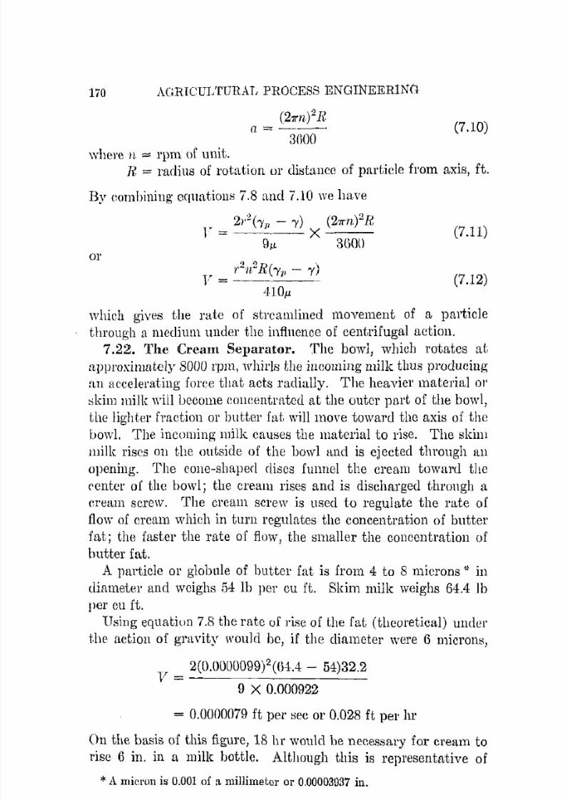
7/16/2019 Engenering Agriculture Perry
http://slidepdf.com/reader/full/engenering-agriculture-perry 179/422
170 AGHICULTlTRAL PROCESS ENGINEERINtt
(21rn)2 Ra=-· - -
3(\00
(7.10)
where I t == rpm of unit.
It, == radius of rotation or dil:ltance of partide from axis, ft.
By eombining equations 7.8 [tnd 7.10 we have
• 2),2(1']1 - 1') (21rn)2R1 = . X-- -
9 -L :3GOl)(7.11)
01' " qR ., i ' ~ n ~ . (/'1' - 1')
l' =-.----4·1Oj.L
(7.12)
which gives the rate of strcamlined movement of a particle
through n mediulll under the influence of centrifugal action.
7.22. The Cream Separator. The bowl, which rotates at
ttpproximately SODO rpm, whirls the incoming milk thus producing
fLU aceclel'ating force that acts radially. The heavier material or
skim milk will become concentrated at the outer part of the bowl,
the lighter fraetion or butter fa t will move toward the axis of thebmv1. The incoming milk causes the material to rise. The skim
milk rises on the outside of the bowl and is ejected through an
opening. The coue-shaped discs funnel the cream toward the
('enter of the bowl; the cream rises and is discharged through a
cream screw. The cream screw is used to regulate the rate of
flow of eream whieh in turn regulates the concentration of butter
fat; the faster the rate of flow, the smaller the concentration of
butter fat.A particle or globule of butter fat is from 4 to 8 microns" in
climnetel' and weighs 54 Ib per cu ft. Skim milk weighs 64.4 Ib
per eu ft.
Using equatiun 7.8 the rate of 1'isc of the fat (theoretical) under
t.he action of gravity would be, if the diameter were G microns,
y = 2(O.0000099)2(fi-1.4 - 54)32.2
9 X 0.000922
= 0.0000079 ft per sec or 0.028 ft per hr
On the basis of this figure, 18 hI' would he necessary for cream to
rise 6 in. in a milk bottle. Although this is representative of
*A micl'on is 0.001 of 11 millimetel' or 0.00003937 in.
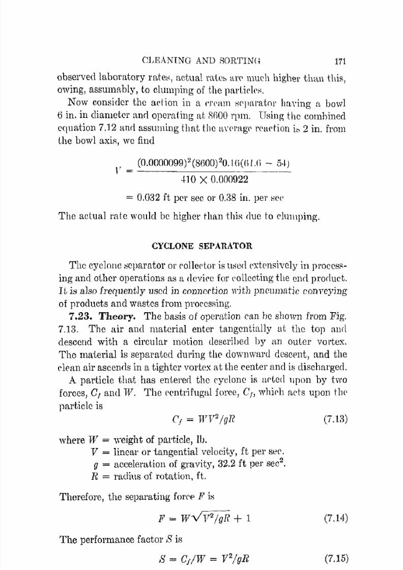
7/16/2019 Engenering Agriculture Perry
http://slidepdf.com/reader/full/engenering-agriculture-perry 180/422
CLEANING AND SORTINU 171
observed laboratory rateK, actual rate:, an' much higher than this,
owing, assumably, to clumping of the p a r L i ( ' l r ~ .Now consider the action in a (']'ram :-lr)laratOl' hrwing i t bowl
6 in, in diameter and operating nt 1\1100 rpm. Using the combined
equation 7.12 and assuming that the ttvrl'agr reaction i::, 2 in. from
Lhe bowl axiR, we find
l ' = (0.ooOOOg9f(8()OO)20.1(i(()l.(\ - ,5+)
+10 X 0.000922
= 0,032 ft per sec or 0,38 in. per HOC
The actuall'ute would be higher than thiR due to clumping.
CYCLONE SEPARATOR
The cyclone separator or ('ollector is used ('xtensively in process
ing and other operations as a dovicc for eoUccting the eml product.
E is also frequently used in connection with pneumatic conveying
of products and wastes from processing.
7.23. Theory. The basis of opemtion can be shown from Fig.
7.13. The air and material enter tangentially at the top aud
descend with a circular motion tlescribed by an outer vortex.
The material is separated during the' downward descent, and the
dean air ascends in a tighter vortex at the center ane! is discharged.
A particle that has eni,el'cd the eyclone is ~ 1 ( ' t e d upon by two
forces, Cf
and lV. The eentrifugal force, C
r, whi('h ads upon tlw
particle is
where W = 'weight of particle, II).
V = linear or tangential velocity, ft per seC.
g = acceleration of gravity, 32.2 ft per see2
•
R = radius of rotation, ft .
Therefore, the separating forC'E' F i:-;F = W ~ + lThe performance factor S is
(7.13)
(7.14-)
(7.15)
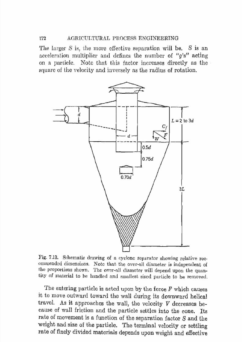
7/16/2019 Engenering Agriculture Perry
http://slidepdf.com/reader/full/engenering-agriculture-perry 181/422
172 AGRICULTURAL PHOCESS ENGINEERING
The larger 8 is, the more effective separation will be. S is an
acceleration multiplier and defines the number of "g's" actingon [\ particle. Note that this factor increases directly as thesquare of the velocity and inversely as the radius of rotation.
IL=2to3d
3L
Fig. 7.13. Sehematic drawing of a eyclone separator showing relative rec
ommended dimensions. Note that the over-all diameter is independent ofthe proportions shown. The over-all diameter will depend upon the quantity of material to be llllnclIed and smallest sized padicle. to be removed.
The entering particle is acted upon by the force F which causes
it to move outward toward the wall during its downward helicaltravel. As it approaches the wall, the velocity V decreases be
cause of wall friction and the particle settles into the cone. Its
rate of movement is a function of the separation factor S and theweight and size of the particle. The terminal velocity or settling
rate of finely divided materials depends upon weight and effective

7/16/2019 Engenering Agriculture Perry
http://slidepdf.com/reader/full/engenering-agriculture-perry 182/422
CLEANINn AND SORTING 173
size. The lighLer and sllwllcr they are, the longer it takes for
them to settle a specified distance. Consequently, the depth or
number of turns in the helix is also important.The actual number of effective turns in a specific separator is
usually difficult to estimate. A safe assllmption for a common
cyclone i ~ t;yQ. but the performing range in many instances maybe less.
I f a symmetrical flow pattern is assumed, the effective cir
cumferential velocity of the outer and inner or descending and
ascending helices can be shown related to the outer 0 and inner i
cylinder diameters by equation 7.16.
(7.16)
The ratio of the performance factors Can then be shown relatedto the diameters thus;
stiSa = doCdo2
- d,2)2jd5
7.24,. Design. Unfortunately, even though the theory of thecyclonic separator is known, few data are available which willaid in the critical design of an efficient unit for a specific job.
The procedures of sect. 7.12 can be used to assisL in designinga cyclone for a specific job. The radial velocity of the particle
is V for terminal conditions, and the gravity factor 9 is multiplied by the separating coefficient S, equation 7.15. The time re
quired to accelerate to this velocity may be considered negligible.
The separating distance is the width of the inlet, and the time
available for separation is the time required for an element of
ah' to move through the effective outer helix. The particle may
be considered as moving in a true radial direction and at the
Bame circumferential velocity as thc carrying air.
Two general types of cyclone separators are recognized. The
common large cyclone, Fig. 7.1 3, is satisfactory for materials
larger than 300 mesh. This would include nearly all the ma
terials that the agricultural engincer would handle. Deep narrowseparators usually installed in banks attached in parallel will
separate such finely divided substances as flour, powdered milk,
fly ash, etc.General relative dimensions for a large-sized cone by Dalla
Valle 4 are shown in Fig. 7.13. The inverted cone placed below
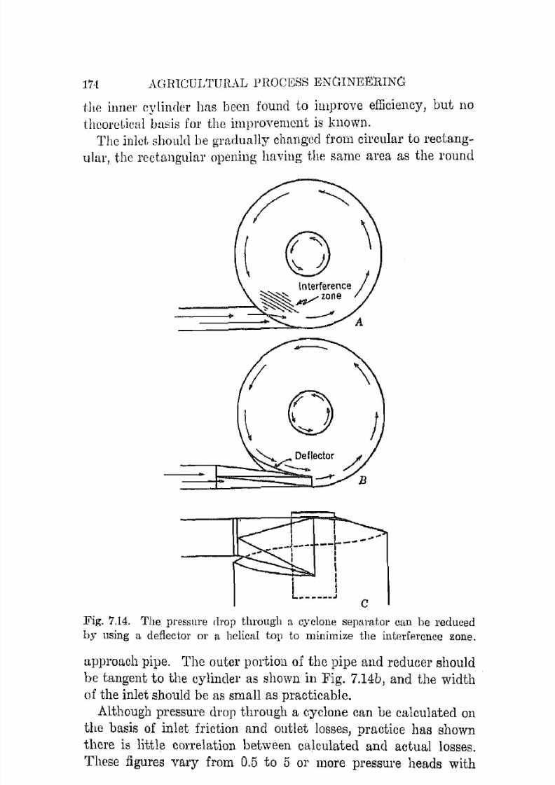
7/16/2019 Engenering Agriculture Perry
http://slidepdf.com/reader/full/engenering-agriculture-perry 183/422
17,l AG.RIClJLTUR"\L PROCESS ENGINEERING
the inner cylinder has been found to improve efficiency, but no
theoreLical basis for the improvement is known.
The inlet should be gradually changed from circular to rectangular, the rectangular opening having the same area as the round
II.. ~ ...- -r - - -II
\I
, II IL _____ J
cFig. 7.14. The pressure drop through a cyclone separator can be reducedby using a deflector or a helical top to minimize the interference zone.
approach pipe. The outer portion of the pipe and reducer should
be tangent to the cylinder as shown in Fig. 7.14b, and the widthof the inlet should be as small as practicable.
Although pressure drop through a eyclone can be calculated onthe basis of inlet friction and outlet losses, practice has shown
there is little correlation between calculated and actual losses.These figures vary from 0.5 to 5 or more pressure heads with

7/16/2019 Engenering Agriculture Perry
http://slidepdf.com/reader/full/engenering-agriculture-perry 184/422
C'LTGANING AND t;(lRTTNG
errors as high as 500 per cent. Intcrfercnce between variOllS
spirals or turns in the air strcHlll within the cyclone is belicved
responsib1e for the deviation. IllLerfcrcnce at the point of airentry is particularly eritical. This l o ~ s ran be reduced by in
stalling a deflector, Fig. 7.14b and/or providing a helical-shaped
top as shown in Fig. 7.14c. These details are not reconllnenclecl
unless pressure drop is an important factor. 1£ the d0flector is
not needed the inlet should he flush with the periphery, that is,
terminated at the wall af! in Fig. 7.14a. Back pressures in helical
top cyclones may be less than 0.6 the inlet velocity head.
Melvin W. First developed an equation for l ) r e S ~ 1 l l ' p loss t,hroup;h a ('yelanc
which appears (0 be a['ceptablc for many cyclones (Fllndamental Factors in
the Design of Cyclone Dust Collrctors, an unpublished the5iR, Harvill'll
University, 1950). This eqnaLion is:
where l ' = J l r ( ' s ~ u r e drop, numher of inlet vclo('ity h f ' l l d ~ .rI = cylindpl" diameter, ft.
L = ryliuder height, ft.I I = rOlle height, ft.
Ii = entry width, ft.h = putry hpight, ft.
E = exit-duet. diameter, rLK = van!' ('oIlRtant, d i l l l ( ' n N i o l l l ( , ~ N .
=zQ)K = 0.5 for no inlet VlLne.
~ ] (= 1.0 for inlet, VlLIle thlLt dol'S !lot expand P!ltf'ring air str('al1lR or\::::!) touch exit duot.~ K = 2.0 for cntry valles that expand pntl'ring ~ ( l " P a m fLml exh'ml from
\:::!) entry t,o exit-duct wall.
Other thl111 these gencml comments al1Ll precautions, no spceific
procedures can be suggestell to insure low pressure losses.
The angle of the main spiral is usually between J00and 150
•
The inlet velocity should be low to minimize pressure 10s:3 and
high for effective separation. Velocities from 20 to 70 ft pel' sec
are usual with 50 about optimum.
Dalla Valle 1 reports work by Rosin, RammIer, and Intelmann,
which gives the theoretical equation for the smallest particle
removed by a cyclone.

7/16/2019 Engenering Agriculture Perry
http://slidepdf.com/reader/full/engenering-agriculture-perry 185/422
176 AGHICULTUHAL PROCESS ENGTNBERING
(
9J.!.d )!:!d' =. 27TNYC,'p - /)(4Rjrl)"
where el' '= ptU'ticle diameter, in.J.!. = viscosity of air, lb per ft-sec.d = diameter of exit duct.
(7.17)
N = number of effective turns of air stream in the innerspira].
l ' = entrance velocity.
'Yp = density of pa.rticlfl.'Y = density of air.
R = radius nt which the spiral velocity is equal to v.
Ie = constant, 0.5-0.7.
This equation presumes streamline flow.
REFERENCES
1. Alden, J. L. Industrial E:-:h:mst Ventilation. Cyelunes and Filters.
lIeating and rent. 35:48-53. July, 1938.
2. Banton, R. Problems in Cleaning Seed. Some Factor.s in Effective
Operation oj Seed Cloaners Using Air and Semells, wit.h Suggestions
1m Corl"ect Use. of Screens for .Man1/ SC})[!r(ttirms. A. T. Fencl! & Co .
Saginaw, M i ~ h i g [ l n . 1946.
3. Cl'uess, W. F. Commercial Fruit anrI Y (Jgotable Pmduc/s. Second Edition. McGraw-Hill. 1938.
'1. Dalla Valle, J, M. Micromeritics. The 'Technolog1J of Fine Parl.icles.
Pitman. Second Edition. 1948.5. Lapple, C. E., and Shepherd, C. B. Calculation of Particle Trajectories.
Ind. Eng. Chem. 32:605-617. 1940.
B. Perry, R. L., et al. Fruit Dehydration. Principles and Equipment.
Calz:f. figr. Eil.'pt. Sla. Bltll. 698. 1946.
7. Roadhouse, C. L., and Henderson, ,r, L. The Market-Milk Industry.MeGraw-Hill. 1941.
S. Shepherd, C. B., and LajJple, C. E. Flow Pattel'11 und Pressure Drop in
Cyclone Dust Collectors. Incl. Eng. Chem. 31 :972-984. 1939.
9. Vegetable and Fruit Dehydration. A Manual for Plant Operators.
U.S.D.A. Misc. Publ. 540. 1()44.
PROBLEMS
1. Analyze or discuss th(J motion of it sieve, Fig. 7.4, with %-in. holes on%o-in. centers, diamond arrangement, from the standpoint of:

7/16/2019 Engenering Agriculture Perry
http://slidepdf.com/reader/full/engenering-agriculture-perry 186/422
CLEANING AND SORTING 177
a. Propel' V lind H for the oseilhting motion.
b. The optimum sereen pitch.
c. StatistiCl\l probability of a seed p a s ~ i n g a hole during a 2-ft downwardtravel.
d. Effect of seed-layer depth on pprforll1l1ncc.
2. A lad ina dover sample weighs 0.100 g per 160 seeds. Assurnc each sred
is cquivalent to a sphere 0.9.5 mm in diamelc!". Estimate the flotatiou
air velocity.
3. A eyliucier separator is 18 in. in diallH'1 ( 'r .
tI . At what rpm would aJl the material be' hdd ill the indents by ceu
Ll'ifugl1l force?
b. At wlmt rpm would it be discharged at 120 0 from the bottom?
'1. A cyclone 6 [1, in diameter with au inlet, 1 it in ciimueler i!l designed us
shown in Fig. 7.13 with L = 2.5d. The inlet is 4 ill. wiele, and inlet
velocity is 50 It per sec.
a. Determine the smallest particle wllj"h CUll be colleetea.b. Estimate the p r e ~ s u r e drop through the unit.
5. Detemline the diameter of a cyclolle' jJroportiolled us I I I the text fuJ'
collecting & I f { ~ l f i : . 7 . l l r e ~ L Caaditians,'
Inlet width
Entrl1neo ai r veloeily
Smallest particlo
Particle fLO.Heparating height
Helix pitch
}.{t CydUl1lJ diametel'
50 ft per SPC
0.0012 in. in dimnptrl'
1.10
1 ~ : ! diaIll!'trm15°
Procedure: Determine the required radial particlo velocity. Calculate
the Reynolds number and find CRe 2• Then combine equa,tions 7.7 and
7.15 and solve for the mdius R which is half th£> rcquil'e'cl diameter.

7/16/2019 Engenering Agriculture Perry
http://slidepdf.com/reader/full/engenering-agriculture-perry 187/422
CHAPTER 8
Materials Hmulling
NOMENCLATURE
"-1 = an empirical COIlHtant, dimensionless.
([. = PI'I'SRure drop, system handling air only, in . watpl'.
B = an ompirieal conShIl(., d i m e l l s i o l l h ~ s s .C = COJlveyor eapacity, eu ft pel' min.
D = Hcrew ui:lmet,CI', in.tI = HluLft diameter, in.
fi' = a lJl:tterild fllet,or, c l i r n e J l s i o n l e s ~ .Fc = codlieient. of frietioll, flights aIllI dmin.
Fm = l'ooffieient of frietion, materil11.
!l = aeeeleration of gravity, 32.2 ft PIll' Hee prl' ';PI\.
II = lifl, ft,.
h = It vurLil'al distall(;<J, ft.
f { = I t variable, rebtell to veloeity.
L = horizontal projedm[ h'llgth of loarlpd cOJlvnym', ft ,
L" = hOl'izontal length, ft.
M = margin, in .
Me = 11 proportionality constt1nt.In = pressure drop, in. water.
N "" revohltions per minute.P = screw piteh, in.
p = velodty pressure, in. water.
Q = material rate, Ib per min.
R = 11 ratio, lb material per Ib ail'.
r "" radius, ft.,..; = l:pntrifug!11 fore(', lb.
t = time, sec.
V = veloeity, ft pel' min.
11 = speed, n per min.IV = unit volume weight, lb.
IV"
=weight of flights and ehain, Ib par ft .
w = flight, width, in .
The perfonnanee of a processing plant is measurably affectedby the efficiency of the movement of materials from one unitoperation to another. The importance of this movement of ma-
178

7/16/2019 Engenering Agriculture Perry
http://slidepdf.com/reader/full/engenering-agriculture-perry 188/422
MATERIALS HANDLING 179
terials is not essentially fL function of itf> magnitude. Efficiency
in delivery of grain \'0 a hammer mill amI rcmoval of the grounrl
product in a grinding job on the farll1 arc ju:;t 11:> important, relatively, as movement of' material through i t packing plant.
I n d u s L 1 · i ~ 1 l materials handling is n highly specialized enterprise
Its procedures and details have developed out of usage and ex
perience in great measure, the rational approach being undevel
oped in many raSCK. Large in:,;tallations should be designed and
installed by materialf>-handling enginc('rf>. Rmanc!", less involVf'rl
installations can hE' designed and installecl by the resident enf!;i
neer uf a processing plant, a local llwcll[mic, or the htruw!".Materials handling as rC'cognized in general implies tIl(' 1ll00'C
ment of materials in ::my direction and, c o n ~ e q u c n t l y , indmles
elevation as well tlR movement in a horizontal plane. Movement
of fluids could be conf>idered unrler this heading, hut since they
have been discussed in the ('hapters dealinp; with fluid mechanics,
flow-rate met1surement, pumps, and fans, fluids will he omitted.
Handling devices may be elassifie(l as follnw:,;:
1. Belt conveyors.2. Chain conveyors.
3. Screw conveyors.
4. Bucket elevators.
5. Pneumatic conveyors.
fl. Gravity conveyors.
7. Cranes.
s. Lift and carrying trucks and carts.
Cranes, trucks, and rarts might be considered as intermittent
r'onveyors. These devices are frequently uReful in providing an
efficient flow of material through f\, plant and, consequently, are
discURsed in this connection.
nELT CONVEYORS
The )wlt ('OIlveyor is essentially an endless belt. operating ue
tween two 01' more pulleys. The belt and it s load are usually
supported on idlers. The installation may be a simple one such
as a light canvas belL sliding over a long table and carries fruit
or a very heavy belt that is supported by ll.utifriction bearings
and carries grain.

7/16/2019 Engenering Agriculture Perry
http://slidepdf.com/reader/full/engenering-agriculture-perry 189/422
ISO AGRICULTURAL PROCESS ENGINEERING
8.1. Cllal'actcl'iEltics. Belt conveyors have a high mechanical
efficiency since, in lnl'gel' installations, all the load is carried on
antifridioll bearings. Damage to the product being transportedis slight since there is little or no relative motion between the
product being curried and the belt.. The carrying capacity is high
since l'elatiYely high belt speeds are possible. Materials can be
conveyed long distances, but there is a limit to the angle of
elevation. A properly designee! and maintained belt system has
a long scrvice life, but the initial cost is usually high. Installa
tion is advisable only when amortization of the high initial cost
('an be assured.8.2. Details. The elements that must. be considered relativc
to belt. eOllveyors are the belt, drive, tension or take-up fcature,
idlers, and loading and discharge deviccs.
Belts must be flexible enough to confo1'111 to the pulleys, wide
enough to carry the qnantity and type of material requircd, have
strength enough to stand up uuder the expected load and operating
tension, and a l'esistaut slll'face. Stitched canvas, solid-woven,
balata, and rubber helts may be used. Stitched canvas and wovenbelts [lrc usually impregnated with a wat.erproofing material. A
I'llhber belt is made of canvas or woven material impregnated
and vulcanized with rubber and covcred wit.h a rubber sheet.
Balata belts are similar to rubber belts as regards aging but are
affected by temperatures over 120°F.
The drive should be at the discharge end of the belt and can
be a conventional belt drive. The pulley must be large enough
to provide enough contaet surfaee with the belt to insure a positive drive. Additional contnet surface may be provided by using
un idler pulley to provide more wrap eontaet of the belt. Pulley
diameters must be large enough to keep from overflexing the belt.
The take-up that is necessary because of stretch of the belt and
of cont.raction and expansion due to changes in moisture and tem
perature can be manual by adjusting screws or automatic by
attaching a dead weight. This adjustment can be on the foot end
pulley or on an idler pulley.The load-carrying idler pulleys, Fig. 8.1, may be plain wood or
light steel for fiat belts or multiple when advisable to provide a
trough to increase the carrying capacity or to confine materials
that would not stay on a fiat belt.

7/16/2019 Engenering Agriculture Perry
http://slidepdf.com/reader/full/engenering-agriculture-perry 190/422
MA'l'EHIALS HANDLING 181
The material can Le fecl uuto the belt by hand or by a mecha
nism that provitlps u. continuous stcady flow. 'This may be a
simple funnel with gate valve or jf the material is not free flowing, an apron, screw, vibrating, Or other type of feeder may benecessary.
!i\g. 81. Troughc(l (l.nel flat idler pulleys fOl' belt conveyors. The straightpulley IS used for Lhe empt.y belt return and infrequently for carrying the
load. (Courtesy Link-Belt Co.)
Tho maLerial 11Jay be rlischarged over the end of the belt, bya diagonal scraper, by tilting of one or more of the idler pul1eys,
or by a trippor. A tripper cOl1bists essentially of two idler pulleys
that cause the belt to take the shape of an S, Fig. 8.2. The
material is discharged over the top pulley anu is caught by achute tha,t diverts it to one side of the belt or the other. A short
belt conveyor operating at right angles to the main belt may re
place the chute if it is desirable to move the material a consider
able distance from the main belt.

7/16/2019 Engenering Agriculture Perry
http://slidepdf.com/reader/full/engenering-agriculture-perry 191/422
182 AGRICULTURAL PIWCESS ENGINEERING
Trippers and scrapers are usunJly movable so that dischargemay be made nt any point on the belt 01' on either side. They
n m ~ be reversible so the main belt cnn operate in either direction.I f discharge is not desired the material is permitted to fall from
the upper pulley back to tlw belt.
F i ~ . 8.2. Open\l,i(\nal lwineipll' of I.lle Il'iJlrwl'.
Disehal'ge by tipping idlers may not be advisable since the
Dmterial is discharged over a considerable length of belt and there
i" an additional stl'nin planeu upon the belt due to twisting. An
angle scraper is the i:limplcst discharging device and is satisfactory
for lllany materiab. The various dischargers are designed so that
they can be controlled remotely.
8.3. Design. The following suggestions are for preliminary('aleulations only. A large belt-conveyor system is an (lxpensive
A=30'
A=20'
Angle of slope
F i ~ . 8.3. Cross section of lotlded belt. showing Lhe sUl'chargc-materit\1
above the dashed line-and the top profile for various slope angles.
and intricate installation and should be designed and installedunder the supervision of specially trained conveyor engineers.
The width of the belt is determined by the size or amount of
material to be conveyed, the quantity to be conveyed, and the

7/16/2019 Engenering Agriculture Perry
http://slidepdf.com/reader/full/engenering-agriculture-perry 192/422
MA'l'IWIALN HANDLINe 183
type of KNVHll'. '1'11(' load ('ross ::;c('tion of a truughed belt is
Hhown in Fig. ~ . 3 ; and Uw areHR of loa(l CrOHi:i flection, in Table 8.1
11(ll\pt eel frolll H etz(,l u}Hl Albl'ighL. l The surcharge is that portionof the load above the level in<iimLkrl by the dotted Hne in Fig.
8.3 Hnd may bo oOlli:iidl'l'od :tR Ute load on a cOlllparu,ble fiat, belt.
The i:iul'eha l'[!,l' angle iH large fo], large lumped materials, particularly i f mixc(l with illle IlltLl,O]'ial, such as mine-run coal. The
20 (\rgI'CO H ] ' ( ~ HhoWH thr' :'nll'fueo pl'oillo of most mlltel'iu,ls.
Examplt·. A troup,Il!'I[ bplL witIl II 20 liegl'ec surcharge i9 to convey 1500
bu of whrllt (411 tOll) I"'\' hI'. What width of helt should he uscd if maxi
lllum opPlnt illg HIII'('([ i9 a H ~ l I l t l ( ' d ' / The ('Itlcllhtt.ion is:
11)00 = (An'n of ('],OHH Hl'l ' tioIl i ll fL X Hpo('(1 il l ft pl'l' m in X ()O)/1.2.5
By trial nll(l ('ITO]', l I ~ i l 1 p ; tlw ( ' l ' O H : ' ; - ~ I ' l ' t i ( ) I l Itn'lt f roUl Fig. 8.3 !Lud the maximum HIWpr[ from 'i'ahl(' H.l for c'I)J1H(,I'uLiv(' 1)(>1[. willthH, !t 14-in. belt traveling
at '100 fL ]H'r mill iH found I ) giv(l
(O.O!)(i X lOll X nO)/1.21) = 1830 hu pOl' hI'
whil'll iH Lhc' [lC'Ht. valul' t () ~ C ' I ( , I ' L .
'l'l.hle iU B l ~ ] ' ' l ' - L ( ) A D (mOSS-SECTION AlmAS ANDMAXIMUM BELT SPEEDS
Total Cl'os.h'Jection Max. Speed,
Clcft1' A1'eft, , ~ I j Jt, Jar Jt 1)81' minBelt Mnrrlin S1t1'!'illLl'(IC Anole it
Width, (M), -- -- - --- ------- No1!abmsiv8
in. in. 100 1200 80° Fine Materials Grain
14 L.7 0.07·1 0,09(1 0.117 300 400l t i 1.8 n.101 0.131 o ,1(J2 300 450
18 1.g 0.1;)4 O. 1 7 : ~ 0.214 400 450
20 2.0 (). 170 0.220 0.272 400 500·
24 2.2 ().257 0 . a : ~ 2 0.410 sao GO O
30 2.5 (J..121 0.;;42 O. {\Oil .550 700
HG 2.S (). {122 0.80;{ (l.9Ol GO O 800
'12 :U O.SH!) 1.12 1.:37 600 800
48 3A 1.W 1.48 1.83 GO O 800
54 :L7 1.'15 1.nO 2.33 GO O 800
no 4.0 um 2,aO 2. !ll (i00 800
Fine fr('o-ilowing materials may be blown or shaken off the
convcyor at high bolt i:ipeetls, particularly i f a fiat belt is used.
Delt, incline is limited to 15°_17° for grain, 18°_200
for bank
run gravcl, and 20°-23° for earth ancllimc.

7/16/2019 Engenering Agriculture Perry
http://slidepdf.com/reader/full/engenering-agriculture-perry 193/422
18,1 AGlUCULTUIUL PROCESS ENGINEERING
The horsepower required for movement of materials by belt
conveyors can be ealcubted by conventional engineering l l 1 e ~ h o d sby considering the lift, the frictional resistance of the belt, and
the frictional resistance of the various pulleys and tripping de
vices. However, the constants used in such a procedure vary with
change in opel'ating conditions; also, flexing of the load and belt
between supporting pulleys absorbs some energy. Empirical data
have been found more applicable than rational data.
The Link-Belt Co.' has found that power for their standard
installations cnn he cnleuln,tccl from the following equations:
Horsepower to drive empty conveyor
= Belt speed, feet per minute (A-+ BL)/lOO (8.1)
L is the conveyor length in feet. Constants.'1 and B depend upon
t,he belt width find are given jn the accompanying table.
Con vel/or BeltWidth, in. A 13
14 0.20 n.nOHO1G 0.25 O.OOl4()
18 0.30 0.001G220 (J.30 0.0018724 O . : ~ f . i 0.0022430 0.48 0.0029836 0.64 O.0039n42 0.72 0.0045848 0.88 0.0053854 1.00 0.00620
60 1.05O.O(J7Gfi
Horsepower to convey matel'lal 011 level
= Tons m[1terial pel' hour, (0,'18 + 0.00302£)/100 (8.2)
Horsepower to lift materiaJ
= Lift in feeL X 1.015 X Tons of material pel' hour/lOOO (8.3)
The total power required is the sum of the powers calculated from
equations 8.1, 8.2, 8.3.Example. In the previolls example, the conveyor is 400 it long and has
11 15° incline; What is the horsepower requirement?From equation 8.1 the power )'('quil'ed to drive the empty "onveyor is:
400(0.20 + 0.00140 X 400)/100 "" 3.0·1 hp

7/16/2019 Engenering Agriculture Perry
http://slidepdf.com/reader/full/engenering-agriculture-perry 194/422
l\L\TERIALS HANDLING 185
From ('(luatioIl R.2 hur:<ppowr'1' J('quirl'li ful' [ ' o ] 1 v [ ' y i l l ~ iH:
45(0.48 + 0.00302 X 400)/100 = 0.70
The lift is 400 I'in 15" = 104 fL. The PO\\'C'I' l'eljuil'E'd to [·jpvate til(' material
is clctc'l'mirwd thus froll1 p q \ U ~ t i o n 8.3:
Thpl'pfnI'P, tll(' tutal hOI'HPPO\\'PI' requilf'lll('llt j "
3.04 + 4.75 + 0.7() = 8.55
This vlllllP dncs not. ill('}udp til(' POWC'1' ]'('cluil'pd fo r iriplWl'1< and uthpl' :1llxilial'YpCjniplllPllt.
CHAIN CONVEYORS
Ch(1in conveyc\n; U8C(1 in ag,ticuUAln\l precessing; 11.1.ay be (:01\.
trastcd to belt conveyors in many ways. Belt conveyors are
expen"ive, r111iet, fast, mechanicflJly efficient, and must be carc
fully enginrered to insure sati;:;faetory performance. On the other
hand, chain c()nveyors are not so ('xpensive, may be noisy, nrc
slol\', al'e not mechanically efficient, and do not require as "peeial
ized skill for deRign. Because of versatility in design and the
adv[tnt.ag,es in(licated abovc, ('hain ronvcyol's are admirably suited
to a greflt variety of materials moving jobs. This is partirulal'ly
true in ngl'icultlll'c whcre servicc is intC'1'll1ittent.
Chain ('onveyors may be classificlI in three ways: (1) trolley,
aIRo calJC'd overhead or lllOllorail, (2) scraper, and (3) apron.
8.4. Trolley Conveyors. This type of convoyor consists of
an ovC'rlwad I-beam track with trolleys that are fastened together
hy chaiu, Fig. 8.4. The trolley conveyor can be used for products
of large uniL size or for those that are handlerl in boxes 01' baskets
at some time during processing. Meat products, fruits, and vege
tables arc examples of materials that, may he handled in this
mnnner.
The direction of motion of a conveyor of this type is extremelyflexible. I t can be designed to make sharp turns up to 1800
•
Stecp elevations can be included in the track, the incline being
limited only by the clearance of the equipment and the load. This
feature is particularly useful where the product must be immersed
in a bath for such operations as blanching, cooking, or cooling.

7/16/2019 Engenering Agriculture Perry
http://slidepdf.com/reader/full/engenering-agriculture-perry 195/422
186 AGRICULTURAL PROCESS ENGINEERING
Fig. S.4. A trolley cOIlI'eyor in n ment processing plant. (Courtesy Link
Belt Co.)
8.5, Scraper Conveyors, Scraper conveyors used for granu
lar, nonabrasive materials are simple, eheap, easily constructed,and may operate at steep inclines. However, power requirements
are high and wear may be excessive.SerapeI' eonveyors are used extensively for moving raw prod
ucts, beets, potatoes, small grains, for example, into processing
plants. They may be permanent or portable, the portable farm
grain elevator being the rnost widely used adaptation.
The types of chain available for conveying are extremely varied.
A simple complete classification 'would be difficult to provide. Themain types, however, are:
1. Malleable detachable.2. Malleable pintle.
3. Steel.
4. Roller.5. Combination.
The malleable detachable chain is the mostC0111111on.
I t is usedfor light intermittent service such as portable farm grain elevators
and elevators on threshing and grain-cleaning machinery. Pintlechain characterized by a pin that connects the links is used for
more rigorous service such as vertical inside grain elevators, beetelevators, and materials elevators for processing plants. Steel
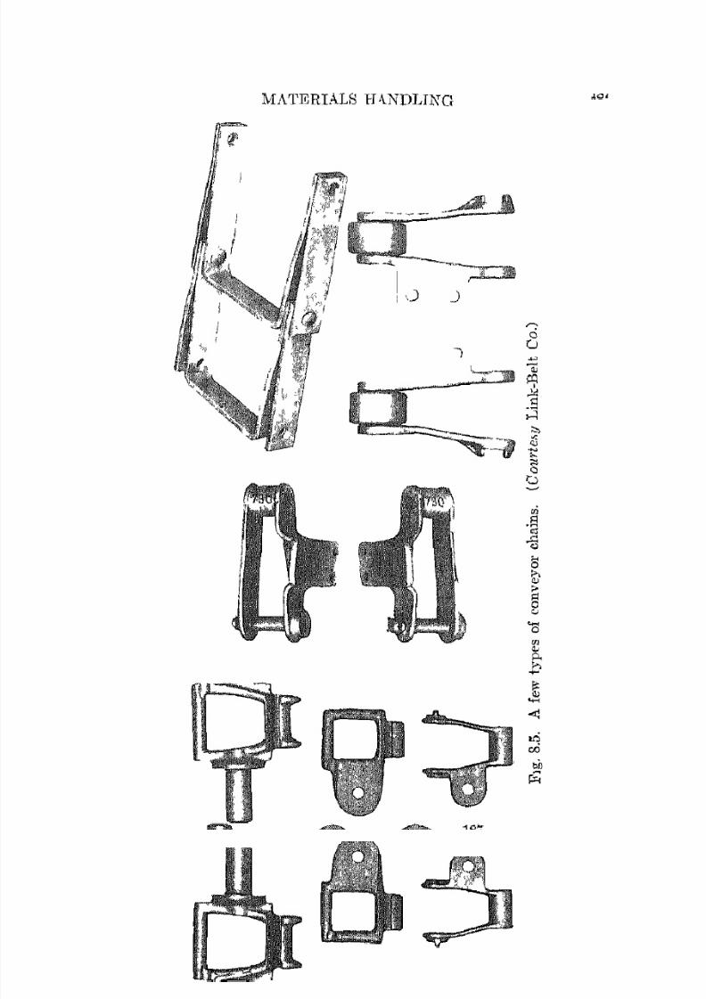
7/16/2019 Engenering Agriculture Perry
http://slidepdf.com/reader/full/engenering-agriculture-perry 196/422
MATERIALS H J\.NDLING 187

7/16/2019 Engenering Agriculture Perry
http://slidepdf.com/reader/full/engenering-agriculture-perry 197/422
IS8 AGR1CULTURAI, PROCESS ENGINEERING
chain is used where high strength or good wearing qualities, or
both, are neecled. Roller elwin is fittecl 'with rollers or wheels to
minimize friction and reduce wenr. Combination cbain is made
in such a way that various features of the above three types are
combined to provide certain definite performance elmraderistics.
Chains of speeinl alloys are available for operation in the presence
of heat, chemicals, ahrasi.ve substances, etc.
~ ~; ~ - = ; : : : : : - -
" r c
(a) (b)
, rtt::::P
T--- - - -
(c) (d)
Fig. 8.B. Cross sections of some scmper conveyors. COlll'f!YOl' a may bemaile of wood, as shown, or ~ t e o \ . If elosell ttt. tho tOll, it may operate in
the normal 01' inv(!rted position. Conveyor b is [ l steel pipe with Il. cylin
drical flight. Power and weal' ' ~ I ' e minimized by HuppOI'ting the flights on
wearing plates c or on rollers d.
A few chain-link types are shown in Fig. 8.5. The lugs aredesigned to fasten to flights of various type, or, in some instances,
to contact the material directly and move it without the benefit of
flights, transfer chain for example. The links may be fitted withrollers that carry the load and minimize fridional resistance.
The simplest conveyor is one made with "sawdust" chain, the
links acting as flights, Fig. 8.5. As the llallle implies, it is used
particularly for removing sawdust from sawing and milling opera
tions, but it cun be used for many other materials such as hulls,,husks, and pulp where the quantities involved are not high.
Scraper conveyors with attached flights are designed in a va
riety of' ways. The simplest of them is a single chain with flights
operating in It wood or steel tl'ollgh, Elevators of this type are
7/16/2019 Engenering Agriculture Perry
http://slidepdf.com/reader/full/engenering-agriculture-perry 198/422
MATERIALS H/\XDLING
usod extensively for moving thc pl'oduets of ffll'lning o p c r a t i o l l ~ .Cross SOPtions of t h i ~ and oUwr cOllveyor:;; are shown in Fig. EU:i.
l'.Iatcl'ials of large granular f-ize arc com'eyed on the top of tlIPconvcyor. For slllall granular matcrial, the lc)\vel' fljghts [Irc 011-
closecl and the material is convcye<l at this point. This llcl'mib
greater capacities boeHutle the trongh can operate full and at a
higher speed than topside movement permits. Also, tho (,11closc(1
feature permitH bigh elevation angles. Discharge for both top
amI bottom-run conveying is ubually at the hpad shaft. How
ever, by putting glltCS in the lower trough, disclml'gr for lower
flight conveying can hc made al any point in thc conveyor. Aimilady, top flight rlil:,e]!::trge can he farilitatecl hy gates in l he top
trough and an open or skelrton lower trough.
S.6. Apron Conveyors. I f the flights in the "craller eonveyort-.
are rrplacerl with flat slats, steel plates, or boards, we have eAsen
lially a moving platform or aprou. This Lype of dcvire can be
u ~ e c l for conveying :;,acked materials and materinls of large unit
size.
S.7. Chaiu Conveyor Design. The following design procedure applies to scraper conveyor:,;, but the student \yill note that
apron and troncy conveyor" ran be rlesigned in fl, coml)arable
manner.
Flight heighL, lpngth, n.nd spacing will depend upon the ex
pectcd duty of the ('onveyor. Flat flights would be l'ecommenrlrr{
fur Racked materin.l, r;hallow flights for large-uniL-size material
Huch as ear corn and sugf1l' beets. For small grains nnrt com
parable materiab, flight height should generally be approximately0.4 the flight length and spaced at approximately the length.
Flight speeds vary from 75 to 125 ft per min. Low speeds
should be used for matcrialii of large granulnr size such as ear
COl'll and walnutb. Slllall granulal ' material such as "mall grain
and clover il(wd can be muved at higher speeds particularly if con
veyed in the lower enclosed portion of 1,he conveyor. High speeds
may damage the product. Where practicable, capacity should be
provided by large-size flights rather than high speeds. The cnpacity of a scraper conveyor operating on the level can be assumed
as 115 per cent of the rectangular space between two flights when
designed as suggested above. rrho capacity 01 a conveyor operat
ing at an ineline will have less capacity than when operating on
the level accorcling to the accompanying tabulation.

7/16/2019 Engenering Agriculture Perry
http://slidepdf.com/reader/full/engenering-agriculture-perry 199/422
190 AGHICULTURAL PROCEHS ENGINEERING
JllcTille, Degrees Apprml:mate Reialille Capadty
20O ~ 7
ao 0.5540 0.38
Thc ndues that, define the relative capacity of the conveyor will
vary cOllsiclel'llbly from material to material. For example, linted
cotton seed will pile much higher on a conveyor than flax seed.
This will affect the relative capacity when operating either level
or at an angle.
Note that the capacity of It conveyor that moves the materialin the enclosed lowcr part of the frame would not be materially
affected hy the angle of inGline. .
The theoretical power requirement for flight conveyors can be
dptcrmincrl from the following rational equation.
2vLcWcP c + Q(LF", + H)HOl'sepO\ver = (8.4)
33,000
where v = speed of conveyor, ft per min.
La == horizontal projected length of conveyor, ft.
We == weight of flights and chain, lb per ft..
Fc == coefficient of friction for chains and flightR.
Q == lb material to be handled per min.
L == horizontal projectedlengt.h of loaded conveyor, ft..
Fm = coefficient of frict.ion for material.
H == height of lift, ft.
Tahle 8.2 FRICTION COEFFICIENTS (SLIDING)
Material
Meti11 on oakOak on oak, parallel fibersOak on oak, cross fibersCast iron on mild steelMild steel 011 mild steel
Grain all rough boardGrain on smooth boardGrain on ironCoal on metalDry Hand on metal
Malleable roller chain on steelRoller-hushed chains on steel
O.W-O.flO0.48
0.32
0.230.57
0.:30-0.45o.aO-0.:350.35-0.40
0.60
0.60
0.35
0.20
Source
Marks
MarksMark:;Marks
Marks
Ketchum 6
Ketchum 6
Ketehum 0
Link-Belt 7
Link-Belt 7
Badger and McCabe 2
Badger and MeCabe 2

7/16/2019 Engenering Agriculture Perry
http://slidepdf.com/reader/full/engenering-agriculture-perry 200/422
MATIGHIALS HAXDLING 191
The calculated horsepower must he adju:oted to COlnpen!:luto for
expected lllaximum load conditions, ~ t a l ' L i l l g fricti()n, loss in the
driving mechanization, variation in frictiOll coefficients, type ofpower unit, ete.
Exatnllle. Design a, steel conveyor with the gmin moving in the open
top to opf'raLe at a 30° incline and rleyutc slicllpr] eorn Lo a height of 18 i tat a rate of 1500 bu per hr.
A ~ , ; u m i n g a flight. Hpeed of 100 ft per min, tlw c : r o F ~ - F e d j o n a l areft of the
scC'tion iR: 1500 btl ] ler hr = 31.25 ('tl it. of grain or 1400 Ih of shpllf'll corIl
111'1' min. The flip;ht width 10 is:
Volump material per minw=-::-c---:::-:--c::-----:-:--=----:=--::-----o
0.4 X Relutive Cltpucity X Flight speed
. 31.25 .w = . = 1.1G ft 01' 14.3 l l l .
0,4 X 0 •55 X 100
Use 15 in. The theoretical Ipngth or run of the conveyor would be the lift
divided by the sine of the iIH'line angle which is
IS/sin 30° or 3/j ft
Additional length must. b(' used to provide cl('arallce Illld overhang at the top
or diseharge end, We shall add 4 f t to take care of t.his * making tht' total]pngLh 40 ft and the total lI('tUtLi lift 20 ft.
The load will create I I tt'm,ion in the chain according to the Re('Olld part of
equation 8.4 thus:
T = Wt material pel' f t (LmF", + H)
= 44.7 X (tfr)2 X 0.4(40 cos 30c X 0040 + 20)
= 946lb
Bec[luse of the width, two chlLins would be required, operating tension in
each heing 473 lb, A chain of 0.902-in. pitch has an ultimate strength of
1250 1b which would provide !1 factor of safety of over 3. This is Ildvisablt'
beeause of possible shock loads resulting from jamming. The chain weighs
0.5 Ib per lineal foot and the Hight abollt 2 lb.
Note should be made that the weight of the chain und flight;; add to the
load and should be included in ihe cnlculations of equation 8.4. H o w ( ~ v e J ' ,since the weight of the chain and flights in this example is small as compared to the material t.o be handled and sinre a moderat.e to high s[lfety
factor is required, weight of ('hains and flights may be neglE'cted in many
*The point of discharge must be sufficiently above the Rpecified plevation
height in order to provide cleftrance for the housing and discharge spout.
This important. requirement is frequently overlooked.

7/16/2019 Engenering Agriculture Perry
http://slidepdf.com/reader/full/engenering-agriculture-perry 201/422
1!l2 AGRICULTURAL PROCESS ENGINEERING
Cll.leulati"us. I f the weight of the material i" low and the chain (lUet flights
~ i g J l i f i ( m n t as compared to tlw rnatel'ial, it will be advisable to include Chern
ill the initi,tl computation. Thus the ]lower requirement is:
2 X 100 X 34.6 X 3 X 0.50 + 1500 X 56/60)(34.6 X 0.'10 + 20)Horsepo\V()1' = 33,000 ...._-
HorseplJwnl' = l.75
A 3-hp unit would probably prol'ide a suitable facto!' of safety.
SCREW CONVEYORS
Screw conveyors are used to handle finely divided powders,
damp, sticky, heavy viscous materials, hot substances that may
be chemically active, and granular materials of all types. Be
cause of simplicit.y, freedom from sharp recesses, cracks, and
crevices, dust-tightness, ane! ease in disassembly, screw conveyors
are used [or moving fOOll product.s such as pmvdered milk and
peanut. but.ter. Screw conveyors are used for batch or continuous
mixing, for feeding where a fairly accurate mte is required, and
for conventional eonveying and elevating jobs particularly where
the run is short. Flights are made of stainless steel, copper, brass,
aiuminulll, cast iron, etc., for hot, corrosive, or mildly abrasive
materials, anc! are hard surfaced with Stellite or similar matcrial
to resist highly abrasive materinls.
Although screw conveyors arc simple and relatively inexpen
sive, power requirements are high and single sections are limited
in length.
The standard pitch screw has a pitch approximately equal to
the diameter. I t is used on most horizontal installations and on
inclines up to 20°. Half standard pitch screws are used for in
clines greater than 20°. Double- and triple-flight, variable-pitch,
and stepped-diameter screws are available for moving difficult
materials and controlling feed rate. Ribbon screws are used for
wet 01' sticky substances. Special cut flight and ribbon screws are
used for mixing, both singly and in comlection with conveying.Horizontal screw conveyors are usually operated in aU-shaped
t.rough, with or without a cover, depcnding upon the type of
service and the characteristics of the material being moved. The

7/16/2019 Engenering Agriculture Perry
http://slidepdf.com/reader/full/engenering-agriculture-perry 202/422
MAT1W,L\.LS H:\NDLING 193
s('rew iC! r,uppol'tccl by brackets at various ~ t a n ( l a l ' d Rpaeings. For
elevating at It fotcep incline, a cylindrical ll(lw:iing iE-, u:-,pd. Thetube is operated full, and no hracket;" arc used heLwel'll the cncl:<l
sinGe they would interfere with the movement of the ll1ittcrial.
The material supports ancI guideR the flight so that sati::Jactory
uperation results if ['h(' conveyor is kept full.
Acrew conveyors are well suited af' fcedcn; or I1wtf'riug device::,
under hinf:, or hopperH. The IJOrtion of the f'crew under the hin or
hopper is mmally designed with half or third pitrh, the hulanre
of the screw full pitch. Thus the main portion of the ~ r r e w operates half or third full, whereas, the llwtcring portion of the screw
operates full.
Concise formula and data iLre not availahle for indivirlnal de
f>ign problellls, anel it is recommended that a specialie-t he COI1-
",ulted when designing and installing IHl'f!,o screW-f'OIWCYO!' Rystcms.
Data that arc available to aStliRt in design aro empirical. Recom
mendations fo1' design of horizontal llonveyors by the Link-Belt
COUlpany 7 arc shown in Fig. 8.7. Thc capacity of a full srrew('ollveyOl' ItS used for feeding 01' ele'\'ating can be estimated from
the following rational equation which iH accurate enough for initial
es tima os.
(D2 - (F)Theoretieal eapacily, ('U ft per hI' = X P X rpm (8.5)
36.0
where D = Het'eW dianwter, in.
eZ = shaft diameter, in.P = scre\v pitch, in. (normally equal to D).
rpm = revolutions per minute of shaft.
The actual capacity will be much less than the theoretical because
of sCl'l'w-housing elearanee, fluid char!\cteristics of material, screw
length, head of material, and elevation or lift. "Vhen speeific
operating data are not available, an estimate of 50 to 60 per rcnt
of theorotical would he advisable.The power requirement of a screw conveyor is a function of its
length, elevation, type of hanger brackets) type of flights, the vis
cosity or internal resistance of the material, the coefficient of
friction of the material on the flights and housing, and the weight
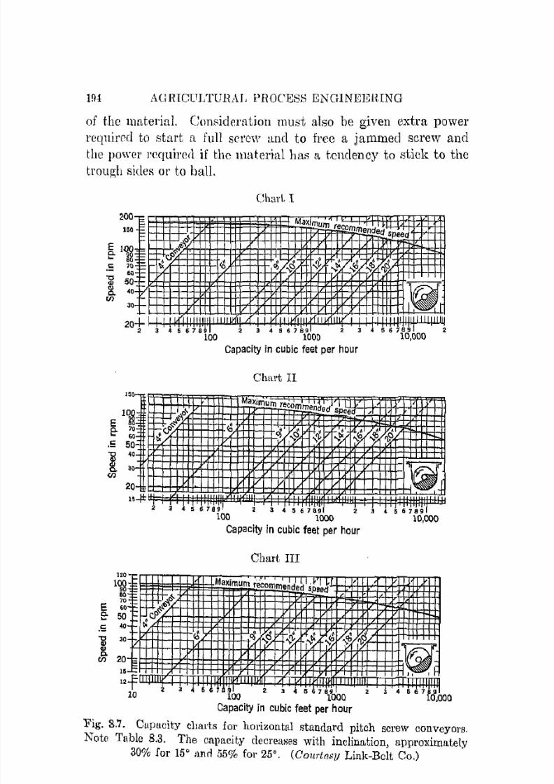
7/16/2019 Engenering Agriculture Perry
http://slidepdf.com/reader/full/engenering-agriculture-perry 203/422
191 AGHICULTURAL PROCESS l!;NGlNEElUNG
of the material. Com:idemtion must also be given extra power
req1lired to start a full scrGW nnd to free a jammed screw andthe POWPl' ] ' ( ~ q u i r e ( l if the mat.erial hns a tendency to stick to the
trough sideR or to ball.
200
I • •
E 100e- ~c: 70._ ISO
~ 50~ 40en
0
~ ~ o <~ if..
0
CharL I
MaXimum recomA mended speed
.Y
~ ' . / ~ -; {:I <t ~ ~ 1 7 ~ ~ Z ~" '" " .." 'l )
~ : .-1- J i U,(L UIIIIIILWII 'TT II iYi'lili, iIW IIII
2 3 4 5 67 . l l 2 5 6 78.10
150 -
0
10QE 3Mc. ,. . 1\0
0
0
.5 50al 4
~ .fl
20,...jl:
guo<!l ',0
lio
, 4 S 6 7 B9 2 , •00 1000 10,0002
Capacity in cubic feet per hour
Chmt II
\ a X i m u m r e c o m m e ~ d e d I I; ,e /
r.; oj)(o ~ i b .$ ~ ' . { ~
]I' 1(jd
2 , 4 5 678g 2 , 4 5 6 76g 2 3 4 •• , . '1
120
1 ~BO
E7060
e- 50
.S 40
..., 3.Q)
8-20/) -I.12
1=10
~ &I!
~
,
100 1000
Capacity in cubic feet per hour
Chart III
Maximum recommenler ~ ~ ~ i ; r
'I I VI
. . . ibo 2. ~ 5 7 "1000 2
Capacity in cubic feet per hour
10,000
• 4 56,..),'.110,000
Fig. 8.7. Cupacity charts for horizontal standard pitch screw conveyors.
Note Table 8.3. The eapacity decreases with inclination, approximately
30% for 15° nncl 55% for 25°. (Colll'teslI Link-Belt Co.)

7/16/2019 Engenering Agriculture Perry
http://slidepdf.com/reader/full/engenering-agriculture-perry 204/422
90
807060
E 50I::- 40
.S 30'C
C1JC1J 20Co( /)
lS
10=f£
60So
40
~ 30
.5 20
I 15
en 109
•
'-cl-"'.;.
d"
-4 S 6769
MATERIALS HANDLING
Churt IV
Maximum recommend d ' ,e speedA' A' IY H-'
:3 4 5 6 7 B ~ T100 1000 10.000
Capacity in cubic feet per hour
ChurL V
, '+1MaXimum recommended speed"
A
I A' ...{
~ LJ_"L ; . f ~ ~ ~ < t Jt) [ ~ i'tL ;; ~2 3 4 5 ,..1 2 3 ' 5 ~ 7 8 ~ ' 1 2 3
10 100 1000
Capacity in cubic feet per hour
Fig. 8.7 (continued)
195
4
The power required to drive a screw conveyor depends upon the
dimensionl:l of the sY!:lcem and the characteristics of the material.
An approximation for normal horizontal operation can be determined from the follo,ving equation.
Hon;epower = CLWF 33,000
where C = conveyor capacity, cu i t per min.
L = conveyor length, ft.
TV = bulle material weight, lb per eu ft.
F = material factor, Table 8.3.
(8.6)
I f horsepower is less than I, double the hor:,;epower; if 1 to 2,
multiply by 1.5; if 2 to 4, llluitiply by 1.25; if 4 to 5, multiply
by 1.1. No 001'1'I::c1.,ion is necessary for values above 5 hp.

7/16/2019 Engenering Agriculture Perry
http://slidepdf.com/reader/full/engenering-agriculture-perry 205/422
tOG AGRICULTURAL l'IWCESS ENGINEERING
TRble S.:i JVIATElUAL CLASSIFICATION AND INDICES FOR
SCREW CONVEYOnS
Material
BarleyBeansBeans, castorBeans, soyBran
ButterCorn, shelledCornmealCotton seed (dry)Cotton seed huliH
Lime, ground
.Millc, driedOatsP()alluts, unshelleuRice, clellll
RyeSawdm;tWheat
Bulk Weight,III per ell jt
38483G
45-5016
5n454025
12603020
15-2045-48
441348
Chart
,NwniJel'
II I
IV
I I
I
IIIIII
IIII I
IIIIII
IIV
I
IIIII
BUCKET ELEVATORS
Hol'sepowerMaterialJi'acto)', Ji'
0.4
0.4
0.5(Ui
0.4
CI.40.4
0.4
0.90.90.6
LO0.4
0.70.4
0.40.7OA
Bucket elevators lllight be classed under either belt or chain
conveyors, or both, since tbey are special adaptations of these.The adaptations arc varied and range from the simple sl11all
capacity unit used in connection with grain-cleaning equipment,to the large, expensive units used for grain, coal, ashes, ete., inlarge industrial plants.
Bucket elevators are very efficient and are more expensive than
scraper conveyors. Efficieney results from the abscnce of frietionalloss from sliding of the material on the housing. It is this
feature that distinguishes the cup elevator from the vel'tical 01'
nearly vertical scraper eonveyor.
Some characteristic bucket elevators are shown schematieallyin Fig. 8.S. The buckets may be enelosed in a single housingcalled H leg, or two legs may be used. The return leg lllay be
located some distance from the elevator leg. A single or double
ehain or belt is used to carry the buekets. The buckets are shaped
with either sharp or rounded bottoms to facilitate discharge (seet.

7/16/2019 Engenering Agriculture Perry
http://slidepdf.com/reader/full/engenering-agriculture-perry 206/422
MATERIALR H . \ ' ~ D L I N n H)7
8.8). They arc f a ~ t c l l e r l to thc helt 01' ehain at the back (Fig.
S ! j i l ) or at, tllC sidc j f two chains arc u6cd (Fig .s NiJ i. Guicb
arc sometimes used for two-rlmin n ~ t a l l a t i o n s , particularly in thc
up leg. Ringle ehains and belt il1lstallations havc no guides or
supports bet wpcn the head and foot wheelb except, perhaps, an
nrl ~ fA~ T
!(
• 0 "•
i "(.
· Ij ,I ~'j r
~ =D !1
.I:(} tJJL(a) (b) (c) (d)
Fig. 88. TIll ee cOlllmon t y p E ' ~ of bucket Plcmtors. (a ) Centrifugal
dIscharge type; m,od f'xtensilrdy for hand ling small grain in c!c\'alors and
processing plants. The buckets are fastE'nrd to a belt. (b ) Perfect-dIS
('hargo type. The buckets !Crt' lIHllally fastellPd 10 a ('ham llnd ojJPrate at.
slow sperd; Lllt'y nre usrd fOJ' mntrl'ials wlmh might hi' damugcri or would
not, stay in h i l ! ; h - ~ p c c d bu<'iwts and for ffll'lIlR wllPre lllitial ('ost mu"t be
low. (c, d) ContinuollH-hllcket LYllC for heavy duty use, 01'1'S, Blind, etr.
Mllteri[1.1 dischargps by sliding, OVP\' hOttolll of preceding hm'ket.
idler 01' two, whieh are placed at strategic points to eliminate
·whip.
S.S. Discharge from Bucket Elevators. Discharge at the
head OJ' top of a bucket elevator is produced in three different
ways as shown in Fig. 8.8. Except for the overlapping buckets,
which are not used extensively in proceSSing, discharge dependsupon centrifugal force in part or in full or the ability of the
material to be thrown into a chute as the buckets go over the
head pulley. The characteristics of this feature and, in particu
lar, the trajectory of the material after it leaves the bucket are
important to proper design and operation, Centrifugal discharge

7/16/2019 Engenering Agriculture Perry
http://slidepdf.com/reader/full/engenering-agriculture-perry 207/422
198 AGRICULTURAL PROCESS EKGINEERING
requires that the ~ p e e d of the belt or chain be held within closelimits in ordcr that the trajectory will fall within the specified
region. An analysis of this follows.Fig. 8.9 shows a head 'wheel and (\ bucket in a series of positions.
A unit mass of grain is subjected to two forces at the point the
bucket starts to turn around the pulley. These forces are the
Fig. 8.9. Force diagram on the grains in a head-wheel bucket in a number
of different positions. The effcdive radius of t.he head wheel bucket varies
frol l l 1'1 to '1'2'
weight of the unit volume TV and the centrifugal force S actingradially which is
s = WV 2 j3600g1'
where W = weight of elemental mass, lb.V = tangential velocity, i t pel' min.g = acceleration of gravity.
l ' = effective radius, ft.
(8.7)
The resultant of these forces R, Fig. 8.9, determines the point at
which discharge takes place and its characteristics.
Note in Fig. 8.9 that R for positions 1-4 is of such a direction
that the material is held in the bucket. At position 5, Sand W
are opposing and R is zero, there being no force on the material.

7/16/2019 Engenering Agriculture Perry
http://slidepdf.com/reader/full/engenering-agriculture-perry 208/422
MATElUALR IlANDLL',n 199
Discharge begins at Lhis point, the initial velocity and trajectory
direction being that of the projected Rpeed of the wheel at this
point, Note thftt R in pOf\itions 6-8 is nearly in the dil'cetion ofmotion of the hucket and tIlU:; forces tlischarge,
In order to prorluce this condition, S amI lV must he equal at apoint, near the top of the travel, or
(8,8)
so that
v2 = 3GOOgl'
and sinceI I = 27T1'N
Where N = revolutions per minute, then
N = 54.19(1/y'r) (8.0)
This equation shows the relationship between the rffective head
wheel radius and its revolutions per minute for the most sat
isfactory discharge conditions, Discharge is not uniform orinstantaneous because the effective l'adim; varies fro111 t ' l to r2 as
i:illown in Fig. 8.0. Thus, the material at the outer edge of the
bucket discharges first.
The chute should be so placed and at such an anglc that all
the material will be taken and at an angle that will minimize
(It'flection. The trajectory can be determined by the following
procedure. The material is discharged in the direction of vector
R which does not haveto
be horizontalus
indicatedin
Fig. 8.9.The horizontal increments vary as vt, t being in small units such
as 0.05 sec. The corresponding vertical distances h arc those of
free-fulling flight or
h = gt2/2 (8.10)
By plotling, the valuoi:l to f:lcale, the approximate line of flight of
a discharged load can be found.
The llletllOcl of piek up in thE' cup elevator is shown in Fig. 8.8.
The foot wheel should not be much smaller than the head wheel
i f the speed of the J l ~ a . . c ; L w l l e e l conforms to the proper discharge
speed. I f the foot wheel is too small, the centrifugal force will
not let the buckets fill. I f it is desirable to use a small foot wheel
a velocity somewhat under that for perfect discharge but which

7/16/2019 Engenering Agriculture Perry
http://slidepdf.com/reader/full/engenering-agriculture-perry 209/422
200 AGRICULTURAL PROCESS ENGINEEHING
will still pl'Ovidc satisfactory discharge should be used. The feed
o:llOllld be so designed that soniC filling \villl'esult after the buckets11l1ye passed above the ('cnter of the foot wheel. The arrangement
sho\\,11 in Fig. 8.Sc is the most satisfactory since only a small por
tion of [,he material gets into the boot proper, most of it being
piekcd up directly from the chute. Note also that if the elevator
stops because of power failure 01' for some other reason, the influx
of material into the bnot is blocked. Consequently, the elevator
can be st.al'tecl without having to (,lean out the hoot.
Fig. 8.10. 'fwo representative buckets. Both buckets are available in a
l'Quge of sizeH. Bucket a hi,,, (l volume. oC 0.104 en f t if 10 in. long, 5% in .
deep (over-all) and projects 5% in. Bucket b lllls a volume of 0.106 ell ft
if 11 in. long ami the Ulln'e radius is 6 in.
The elevator buckets vary somewhat in shape and size but con
form in general to the two shown in Fig. 8.10. The top angle and
the rounded bottom facilitate filling and discharge. The individ
ual manufacturers furnish complete nata on the various buckets
whieh they manufadurc. These data should be consulted for a
specific job.The ccnter spacing of buckets varies with their size, shape,
speed, and head and foot wheel diameter and is specified by the
manufacturers for the various operating eonclitiollS. The buckets
must be placed so that the centrifugal discharging grain does not
hit the hucket ahead of the one discharging. In general, the spac
ing will be from 2.0 to 3.0 times the projected width.
The theoretical power requirement is:
Horsepower = QH/33,OOO (8.11)
where Q = amount of material handled per minute, lb.
= belt speed in feet per minute times number of buckets
pel' foot times capacity of bucket in pounds.
f1 = lift/ ft.

7/16/2019 Engenering Agriculture Perry
http://slidepdf.com/reader/full/engenering-agriculture-perry 210/422
MATERIALS HANDLING 201
The theoretical hon,epower shoul() be increased 10-15 pel' cent
to provide for friction and power l'eflUired for lmtding. Also, if
starting under load or if heavy peak 10arl conditions are frequently expected, additional power should be pl'oYided.
Take-up for chain-wear and belt-tension adjustment are usually
provided by moving the foot pulley. The power shoulrl be applied
at tl1C' head pulley.
PNEUMATIC CONVEYORS
The pneumatic conveyor moves granular material in a closedduct by a high-velocity I:ltrcam of air by Rystems such as shown
? " _ _ : = ~D
IG
IF
IE
Fig. 8.11. PncllmaLic cOllvf'ying :;ySlOlllS. The lllllterial lllay be suclwd up
by It flexible ho ,c, A, muy be introduced into th" intake pipe or direcily
into the fllll by gl'lwity tlow or a hopper, B, Ot ahead of the fan, C. 'flip
maLerial lTI[iY he collef'ted by u cyclone, R, or disehargcd directly. F.
in Fig. 8.11. The advantages are: relo.tively low initial cost;
mechanical Rimplicity (only one major moving part, the fan) ;
conveying path can be random and may branch; conveying path
can be changed easily; a wide variety of materials can be con
veyed (dusts, fibers, sanel, grain, rags, cotton, etc.), and the
Hystem is self-cleaning. The disadvantages are: high power re
quirement (md posHible chlluage to conveyed materials.
Conveying engineers are not in complete agreement as to the
performance and design aspects of pneumatic conveying. Thefollowing treatment prepareu. from various sources 2,5 ,9 ,11 is lJe
lieved by the authors to be adequate for average design.
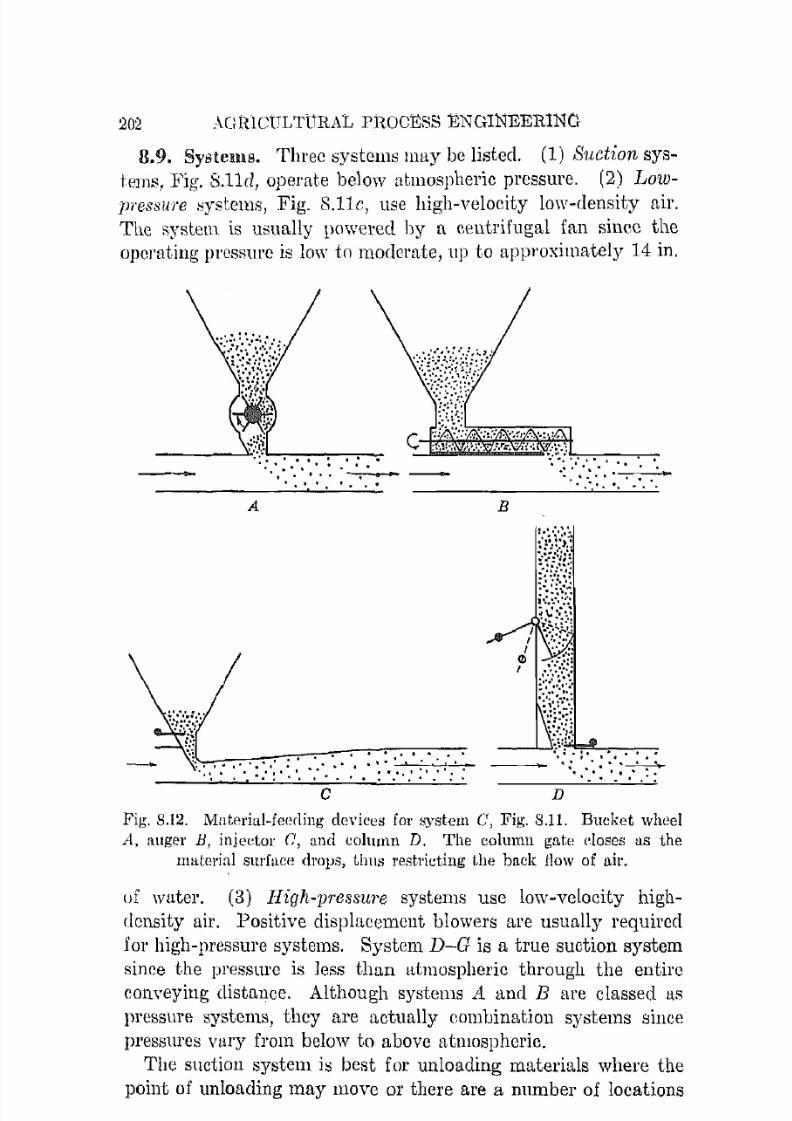
7/16/2019 Engenering Agriculture Perry
http://slidepdf.com/reader/full/engenering-agriculture-perry 211/422
202 AGlUCtTLTURAL PRoCESS ENGINEERING
8.9. Systems. Three systems may be listed. (1) Su,ct7:on sys
I.ellls, Fjg. 8.l1d, operate below atmospheric pressure. (2) Low
pressilre :>ystems, Fig. 8.11c, use high-velocity low-density air.
The system is usually powered by t1 centrifugal fan since theoperating prcsRure is low tn moderate, up to approximately 14 in .
• • I • I ' •
' . . . . '.I • t •• --.---..--....
'. ' ' . ' ..A B
,/~ - - ~ ~ . ~ . ~ . ~ . ~ . . ~ . ~ .~ : . : ~ . : : ' , ••;.:.: • •• ,t I" ': ' .: . , . ' : •• : , : ' :
cFig. 8.12. Material-feerling devices for system C, li'ig. S.l1. Bucket wheel
A. auger H, injector 0, (lnd colulllIl D. The column gate doses us the
lIlaterial surfllce drops, thlls restrieting the back flow of air.
uf water. (3) Iiigh-pressw'e systems use low-velocity high
density air. Positive displacement blowers are usually required
for high-pressure systems. System D-G is a true suction systemsince the pressure iR less than atmospheric through the entireconveying distance. Although systems i1 and B are classed us
pressure systems, they are actually combination systems since
pressures vary from below to above atmospheric.
The suction system is best for unloading materials where the
point of unloading may move or there are a number of locations

7/16/2019 Engenering Agriculture Perry
http://slidepdf.com/reader/full/engenering-agriculture-perry 212/422
MA'l'ERIALH HANDLING 20:1
from which matprial is La he taken. Unloading from trucks,
wagons, freight cal's, and boaLs arc example:;. The ;;:uction systelll
is also best for llIfLtl'rials of such a tt'xturr that they would not
pas:=, easily through valves, HCl'CW fceders, or fans, cottOll, for
example. The pressure I-lystelll is morc efficient than the suction
flystem sincc the eOl1vC'ying ail' density is higher and velocity
lower. I t is best adapterl for work wherc the point of f\i:=,charge
varies. Loading freight CHrs or f-tllrage t,Hnk;:; are examples.
TIH' method or device user! til feed the material into the ail'
:-:tl'eam iH important OWill{; to the effed on the material itself ilml
the power requil'P(l. In addition to the deviN's of Fig. ~ . l 2 thematerial may be intl'orluced into the fan inlet or sucked into the
intake as in Fig. S.llA, B. The pOHsibility of f::tn damage lllU"t
he recognized in the last two procedurrs.
8.10. Air Rate and Volume. An acr'epted material convey
ing rate is 50 ft per Kec. For vel'ticalll1ovcll1ent the air velocity
must bc that to just sup]lort the particlcH pIns 50 ft pel' sec. A
higher material velocity is nerried for horizontal conveying sime
high tl1l'bulrnee is required to maintain the material in s u ~ p e m ; i o n .The air nttc may be less since the air-particle slip is less for hori
zontal ll1ovement. The proper air rate for lifting can be calcu
lated by the aerodynamic procedure of sert. 7.12 or by empirical
methods such as those of Hudson." Hudson's recommendations,
haser! upon the observed performance of many im,tallations, in
clude vcloeities for horizontal ('oIlveying and flexible pickup hoses
and are given in eC(uation 8.12 amI Table 8.4.
(8.12)
where V = air velocity, ft per min.
Me = a constant, Table 8.4.
W = bulk density, lb per ('u ft.
'rl1hle 8.4 VALUEH OF M,. FOR EQUATION 8.12
Material
DustyGrainsGrittyalld uneven
StraightIIorizontal Ducts
Line
101215
Hose
Hi2024
Ducts withElls and Risers
Line
12.501518.75
Hose
202430
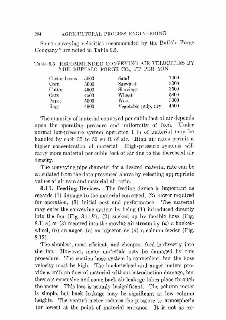
7/16/2019 Engenering Agriculture Perry
http://slidepdf.com/reader/full/engenering-agriculture-perry 213/422
2(H AGRIC(TLTUHAL PHDCENH ENGINEERING
Some eODYeyillg velocities l'ceommcnded by the Bufi'::ilo I ~ o r g eCompany" are noted in Table 8.5.
Tallie 8.5 RECOMMENDED CONVEYINO Am VELOCITIES BYTHE BUFFALO :FORGE CO., FT PER MIN
Castor beans 5000 SrUlfl 7000
Corn 5500 Sawdust aoonCotton 4500 Shavings :3500
Oltts 4500 Wheat 5800Paper 5000 Wool 5000l{ags 4tiOO Vegetable pulp, dry 4500
Tho quantity of material convoyed per cubic foot. of air dependsupon the operating pressure and uniformity of feecl. Undernormal low-pressure system operation 1 1]) of material may be
handled by each 35 to 50 eu ft of air. High air rates permit a
higher concentration of material. High-pressure systems will
carry more material per eubic foot of air due to the increased air
clensity.
The conveying pipe diameter for a desired material rato can becalculated from the data presented above by selecting aPl1l'0priate
values of air rate and material air ratio.
S.II. Feeding Devices. The feeding device is important as
regards (1) damage to the material conveyed, (2) power required
for operation, (3) initial eost and performance. The material
may enter the conveying system by being (1) introduced directly
into the fan (Fig. 8.llB) , (2) sucked up by flexible hose (Fig.
8.llA) or (3) metered into the moving air stream by (a) a hucketwheel, (b) an auger, (c) an injector, or (d) a column feeder (Fig.
8.12) .
The simplest, most efficient, ftnd cheapest feed is directly into
the fan. However, many materials may be damaged by this
procedure. The suction hose system is convenient, but the hose
velocity must be high. The bucketwheel and auger meters pro
vide a uniform flow of materiul without introduction (lamagc, but
they are expensive and some back air leakage takes place throughthe meter. This loss is usually insignificant. The column meter
is simple, but back leakage may be significant at low column
heights. The venturi meter reduces the pressure to atmospherio
(or lower) at the point of material entrance. I t is not as ex-

7/16/2019 Engenering Agriculture Perry
http://slidepdf.com/reader/full/engenering-agriculture-perry 214/422
MATEHJAI,S HANDLING 205
pCll::live [18 the l1wchaulcnl feeders, even though it necessitatesaLirled power at the bIl.
8,12. Operating Pressure. The operating or fnn pressurediiIerentia'! is composerl of (1) air-pressure 10::;8 in pipe and fit
tings, (2) material-pipe friction, (3) material-air friction, (4) ma
terial aceoleration, awl (5) sundries such as occurs in cyclones,
valves, material meterR, etc. The toLal pressure is the sum of the
individual pressure differentials from the sources noted.
1. The pressure loss in the pipe and fittings can be calculated
by any conventional method such a:::; that of Chap. 2. Friction,
elbow, and wlncity losses must be included. The effect of material collectors, vrnt1ll'i or other feeding devices, transfer valves,
and other sundries upon the pressure loss lllUl:.t be included in
the cnlculai,ions.
2. The mechanieB of the loss due to malerial moving in the
pipe arc not well known. The friction of the material against
the pipe is prohably significant for horizontal movement but not
so important for vertical movement. Aerodynamic loss is prob
ahly high for verLical movement, but pipe-material friction isprobahly of littlr importance for horizontal movement.
The BuiTalo Forge Company n uses the following expressions
lleveloped from tests oy M. (iasterstt1clt 3 to (letermine the pres
Bure 10RS resulting from the presence of the !l1u.terial when moved
horizontally.
(8.13)
where rn = tobl pressure drop through a system handling materiali.n horizontal pipe::;.
a = presBure drop through thc system handling air only.
R = ratio, lb material per Ib air.I ( = tt variable that d e p e ~ c l s upon velocity as noted below.
Veloclty, ft 1)('1' min
K
2000
1.15
3000
2.14
4000
3.11
5000
3.5
(jOOO
3.5
The resistance characteristics for vertical movement are not
"vell known. The Buffalo Forge Company U uses a vertical re
sistance twice that for horizontal movement for moderate lifts
(approximately 50 ft or less).
7/16/2019 Engenering Agriculture Perry
http://slidepdf.com/reader/full/engenering-agriculture-perry 215/422
20(; AGHICULTURAL PIWCESS ENGINEEHING
:i. Energy loss in elb01cs cnn be estimated by the equivalent
length of yerticul pipe which is thcn applied to equation 8.13.
4. The energy required to accelerate the material from zero tothe conveying vcloeity is significant. The pressure loss resulting
from the introduction of thc material into the stream of moving
nil' may be estimnted by the following expression ,,,hieh was de
veloped by Gasterstlidt.
1n = 2.25Rp (8.14)
where m :::: pressure loss, in. water.
R :::: ratio, lb material pel' III air.p ::: velocity pressure, moving air.
GRAVITY CONVEYORS
Omvity conveyors consist of a series of rollers 01' wheels set
level or at a slight incline to handle boxed materials in particular.
The material moves by gravity, or by hand if the conveyor is
level. I t is espeeially adnpted for intermittent service.
CRANES
Outside of the cunventional rope huy hoist used for stacking
and barn filling, cranes are not used extensively in agrieultural
processing. They may be used in isolated instances, but their use
is not general enough to warrant more than this passing comment.
LIF'l' AND CARRYING TRUCKS AND CARTS
Much of the processing clone on farm products is concentrated
into a relatively short period during the year. The cl'itieal ele
ment in the flow of materials through a processing plant is usually
the peak of receipt of raw material. Vegetables and fruits have
to be delivered at the most optimum time. The daily peak rate
of receipt is usually higher than the maximulll processing rate.
Consequently, the material mny have to be unloaded and storedtemporarily before starting through the plant.
Furthermore, many plants operate only a portion of the year
and consequently have to minimize ovcrhead as much as possihle.
Rather than buy an expensive maehine for a eel'tain unit opera-

7/16/2019 Engenering Agriculture Perry
http://slidepdf.com/reader/full/engenering-agriculture-perry 216/422
MATERIALS HXNDLINn 20i
tion that is perfol'lllC'rl only a few dayl'i ant of the yeul', ii lllay Ile
economit'ally advifmble La UtiC a slower proros;, taking a lung0r
timc. This in turn woul(l require a change in the rate of move
ment through the plant which would probably require temporary
interruption or storage of material. Com:equcntly, COIlv('utional
continuous-fiow l1l'oredures woulrl not apply ~ u t i ~ f a c t o r i l y .The proceBtling eharneteribtics of uny one plant vary 1'1'0111 year
to yenr and from day to day. For example, incoming [tpplcc> au
a t'ertain clay may grade out 10 per cent for cider. The following
day apples from another source may grarle 2fi per eent eidcr. I fthe plnnt docs not have u cider mill of fiufficicnt eapacity to
handlc the quantity at the rate reeeiverl, tcmporary holding willbc nccessary and normal-flow proeedures will bc clil:irnpterl.
Bccause of these unique aspects uf agriC'ultural p r ( J t ' C ' f i ~ i n g , that
is, possible llny-to-clay variationR in quantity and quality of
material receivcd, the neC'cssity for u minimum overhe[1,cl, and
variation in clireetion and rate of fiow through the plant, a com
plete permanent conveyor system lllay be inadvisable. ThiB (loeB
not prcclude the advisability of permanent installations in mllny
plants or connecting most of the operations in anyone plant. The
most suitable flystem can be determiner[ only after a careful over
al l study of the enterprise. <f
Carts, dollies, and trllckH may be Hatisfartory for handling llla
terial under these conditions. Labor efficiency is possiblc only
whell these devices arc fittcrl to the work in the most satisfactory
manner. Lifting by the operator should be minimized, the ('urt
or truck should frt. the matcrial to be moved fiO that cadi loa<l
will be balanccd for easy movement amI a maximum load willhe carried each Lrip. I f the material is handled in boxe:>, pffieiency
is provider[ if the hoxeti nest so that the rc:=mltant loarl moves as
n unit.
For ll1()(lerai.e, large-size opemLiulls with a high anllual utle
factor, a l i f t tJ'llrk with pallets cletligned to handle the material
is a fai:lt amI efficient device for materials handling where the
speed and direction of movelllenL varies from day to day. Pallets
nre designed in various ways and lllay be platforms, racks, boxes,
etc. The chief feature to considcr is the method of attachment
to the truck.
*Note Chapter 14.
7/16/2019 Engenering Agriculture Perry
http://slidepdf.com/reader/full/engenering-agriculture-perry 217/422
208 AGRICtTLTU.RAL PROCESS ENGINEERING
The lift-trlld::-pallet system of matcrials handling is n ~ l ' y cf
G<·ient for certainl l l t a ~ e s
of mnny agricultural processing operations. I t :-110\11<1 be considered for use wherc the flow rntc is
intcrmittent, and whcrc bags.. hales, hampers, boxes, and similar
largc units lHO handled.
REFERENCES
1. Alden, J. L. Desi(lll oj Industrial E:r/;allst Systems. IndllRLl'ial Press.
1939.
2. Badger, W. L., and l\lcCab8, W. L. Elemcnts of C/wmica/ Elluillcl'6n(J.S e ~ o n r ! Edition. McGraw-Hill. H136.
;3. Gnsterstadl.. M. ExperiIllPIl1al Investigatioll of Pneurnatie Conveying
l'roee,s. ZcilRchrift, des Ve)'einrs Deutsche), Inycnicul'C. llS.. p. \)17-
624. Junc 14, 1\)24.
4. Hetwl, F. Y., and Albright, R. K. Belt Conveyors and Belt Ele'/)(.t!ol·s.
Third Editioll. Wiley. 1941.
5. Hudson, W. G. Convellurs ond Related Rljllipmcnt. Wiley. 1944.
6. Ketchum, M. S. The Desion of Walls, Bl:ns, and Grain Elr.va/.ol's.Third Rllition. McGTl1w-Rill. 191\).
7. Link-Bell Genoral Catalogue 800. Link-Belt Co . 1939.8. J,ongho\lse, A. D., at al. The Application of Fluidization Lo Conveying
Grain. A Progress Report. Aol'. Eng. 31 :349,352. 1950.
9. Madison, R. D. Fan Enginem'inl]. Fifth Edition. Buffalo Forge Co.1948.
IO. Rex Conveyors and ProccHs EClllipment. Catalogue ,145. Chain Be]!;
Co. 1915.
11. Segler, G. Pnenmatic Grain ConveNing with Special Ne/Cl'ena! 10
A(Jl"icultural Applicat.ion. National InsHtute of AgriculLnt'al Engineer
ing. Wrest Park, S i l ~ o e , Beclfordshirc, Engh1ud. 1951.
PROBLEMS
1. Shelled dent COl'll is tu be conveyed '10 i t horizontally and lifted 5 ft
Yertically at :1 rute of 1200 bu per hr.
a. SjJceify 11 scrt'w conveyor, its ~ l J r ~ e d autl horo;epower.
b. Specify a steel scraper flight. eonveyor, its speed I l l l t l h o r ~ e J l o w e r .Two chains are used; chain wl'il4hs 1/;{ lb pel' ft. Flighls are o/tn ill.
thick [Lnd tr:LVel 100 ft per min. What percentage of th e roquired
power is due to the Hight and chain friotillll?c. What power would be required in (I» if roller chain, Fig. SA, with a
coefficient to friction of 0.06 were used? vVlmt is the reduction inper cent.?
2. Whe[Lt is to be moved 400 ft horizontally by a belt conveyor at a rate
of 3000 bu per hr.

7/16/2019 Engenering Agriculture Perry
http://slidepdf.com/reader/full/engenering-agriculture-perry 218/422
MATERIALS HANDLING 200
a. Specify til() bolt wil\Lh, sUl'l!hal'gn angle. bPlt sIJred, and jJowel' l'G
quired.
b. How mueh power is llbsOl'berl in [lccl'ieratillg the graiu'! Till' grainis moving 90 fj , put' min .horizontally when it hits the belt.
3. BUl'kC'tA geometrically ~ i m i b r to Fig. 8.l0a are 12 in. long and nre ;,pacecl
3.0 t i m c ~ thc projp(·( ion. The lift. is 80 ft.. The IJl'ad wheel is 24 in.in tlifllllC( (21'. Dc( { ' l ' l l ] inC' :
(T. Bpi!' "pp('rl {m c('utrifuglll disehuxg('.
b. Capacit.y in llllshris ]If'r hom.
c. IIorsC'powor whrn I'If'vnting shelled (·urn.
4. Plot. the , l i ~ e h a r g c Lm.ic-dory [01' jJl'llbll'lIl a 01' 1'1 nIHIl''] (Fig. FUl). ] )0( ' ,thc grain "omp\P(ely ('It'lli' (lip (li"eiJargcd bllckf'ts? Skcieh the null incof the llis('h[lrge ehul c.
5. A 1 1 1 l ( ! l I m l l t i ( ~ ('onn'yor lllURI. lift, wl1mt 35 £\ all(1 mOVl) it, hOl'izontt\l\y
GO ft at 500 1m per hr . The systcm is A-Ji' of Fig. 8.11. The h o ~ e is
10 i t long. Thc rfLdius of the "IIi:! is 6 tillws the pipc [liametpr.
Determine:
(1 . Hose nIHI pipu difLllwtpr (use 40 C1I fL ail' PCI' pound of mat ['rial).
b. PI'CHSUl'e drop :t('ro,s illE' fan.
(! . Ail' harsC'jJowC'I'.
G. Determine the h01'sC'power for n RUmpel' conveyor far the job of pl'oLlerll
5. ARRllme ~ L e c l ('oIlsLrl1ction; flight llnd chain weight. 2 Ib PPl' lineal
foot.; i1il!:h t spPC'd, 100 ft. ]lCl' min.

7/16/2019 Engenering Agriculture Perry
http://slidepdf.com/reader/full/engenering-agriculture-perry 219/422
CHAPTER 9
He<lt TI'ansfel'
NOMENCLATUltE
A = eI'OSH-seet,ional an'a, sq ft..
e = tt COIlHtanLc = s p e e i f i ( ~ heat, Btu per III of.
D = (iimllot(!r, [t-
O = Vy = !lIIlSS mte, lb per (hI' sq fl.).
It = Rurhee thermal eonductlln(;e, Btu per (sq ft hr OF).
[ = mrlittut-(;nergy rate, Btu Iwr (lir sq ft steradians).
= therIlliLl l ~ o n d u d i v i t y , Btu per (hr sq ft of per 1'0.L = thickuess of a COIlliuotillg layer, ft .
N = cylinder length, ft.
q = lwat nita, Btu pel' hr.
He = Heynolds number.l ' = radius, ft .
'/ ' = absolute tempcmtllre, OR.
t = temperature, of ,
tltV = average tcmpemturc, °Il'.
te = center temperature, of .t / = fluid film temperature, aF.t" = 811rf!t(;C temperature, of .
U = over-all or composite eonduetivity, Btu per (hr sq ft OF).
V = velocity, ft per sec,
'p = volume, eu ft .TV = total emissive power, Btu pcr (hr sq ft.).
JVb = black-body erniHBive power, Btu per (hI' sq ft).
lV/J),. = spectml e m i s ~ i v e puwer, Btu per (hr sq rt micron).
111 = fluid weight, III per hr.
T ' " distance through cOlldueting llwdiuIl1, ft.l/, z = coonlillaLe (lxis, ft.
a: = absorptivity, a. ratio.= monochromatic: a b ~ o r p t i v i t y , It mtio.
fj = coefiieient of cubical cxpa.nsion, en ft per eu ft OF.
l ' = total irradiation, Btu per (hr;;q ft).1\ "" monochromatic irmdiatioll, Btu pel" (hl" sq ft mieroll).
E = emissivity, [ t ratio.
E) . '" monochrollmtic emissivity, a ratio.
y = specific weight, lb per eu ft .
/) = time, hr.
210

7/16/2019 Engenering Agriculture Perry
http://slidepdf.com/reader/full/engenering-agriculture-perry 220/422
HEAT T1L\NSFER
A == way£' if'lIp;th, microllR (orH' mi"ron = o.om 111111).
Jl = vis('oHity, III pCI' ft-RPC.
P = refiectiviLy, a ratio.p>. = monochrornati(' r d l p ( ' l i v i l ~ ' , a ratio.
I I = a conRtallt, 0.173 X ]()-R Btu lwr (hI' 1't °FI).
<P = angle, degrc('s.
if; = a function of.
w = solid angiE', sf ('radian".
211
TranOJfcr of heat is the principal unit operation in tile' rH'oeeb:;
ing of many farm pl'OritH'tH, for example, paste1ll'izatioll of milk
and fruit, juicetl, freezing of f ( ) o d ~ , cooling of fruits and wgetablm;
fut' transportation and storage, and thermal BtcrilizaLion of canncclfoods. Heat tram;fer is also an et-;sentiul operation in providing
the energy for vaporization ill l'vaporation, (liBtillatioll, and dry
ing. UeaL lllUBt be supplied to maintain dei'irablc telllpcraturrB
for lmctcrial growth ill cnttage-eheeKc making; on the other hand,
it mu:;,t be removcd to (woid undesirably high temperatures in
fermentation processes.
Heat energy iR trnnsferrcd by thrce l11cchani:-;]1l!': cOIUlurtion,
convection, nncl radiation. In many systems, all three operatesimultalleoutlly. Superficial consideration of such systcms has
often yielded rule-oI-thumb cxpressiolls that are ohviously simple,
but which have a limited range of application. Sound t r ( ~ l l . t m ( ' n trequires a recognition of the pn,rL playefl }IY each pertinent mech
anism_ The range where simplifications arc valid ean then lIe
established.
9.1. Conduction. Transfer of heat energy between adjaeent
molecules, not dependent on gross movement of material, is calledC'oncluctinn. Substances have the ability to cunduct heat in any
state, solid, liquid and gaReons. In experiments to measure con
duction properties of fluid;;, special care must be taken to avoid
gross movement.
The rate of hrat transfer by ('onductiun through a suhHtance is
directly proportional to the temperature gradirnt, dtjdx, and to
the eross-scetional area of the path, thus:
q = -7cA.(dt/d:r)
where q = heat rate, Btu per hr.
A = cross-sectional area of flow path, sq ft.
t = temperature, OF.
x = distance through conclucting medium, ft.
(9.1)

7/16/2019 Engenering Agriculture Perry
http://slidepdf.com/reader/full/engenering-agriculture-perry 221/422
212 AGRICOLTllHAL PHOCEi-:S ENGlNEEnING
Tllhle D.l COEFFICIENTS Or.' TltERi\lAL CONDUCTIVITY OF
VARIOUS IvIATEH.[AU' *Btu per (hI' sq ft °F per ft )
ApparentDensity,
Matm'ial lb 1)el' euft OF k
Ail' 32 0.0140AshcHtos, cement hoards 120 68 0.4aAsbestos sheets .55.5 124 0.096AsbestoR 36 :32 0.090
35212 0.111
Aluminum :32 117Aluminum foil, 7 air spaces pel' 2.5 ill. 0.2 100 0.025Brick, building 08 0.4Cardboard, corrugater! 0.0:37Concrete 1: 4 dry O.MConcrete, stone 0.54
Copper, pure ()4 224212 218
Cotton wool 5 8f.\ 0.024Cork, hoard 10 86 0.025Cork, ground 9A 80 0.025Diatomaceous earth 27.7 399 0.006
27.7 1600 0.0\-12Fiber insulating board 14.8 70 0.028Glass, bora-silicate 139 86-157 0.f13Glass, soda 0.3--0.44Glass, window 0.3-0.61Ice 57.Ii H2 1.:3Iron, wrought 64 :34.9
212 Cl4.6Iron, cast 12n 27.6
216 20.8Mill shavings G.O:33-0.05Mineral wool 0.4 86 0.0225
19.7 86 0.024Sawdust 12 70 0.03Snow 34.7 32 0.27Steel, mild !14 26.2
212 25.9Steel, stainless (18-8) 932 12.4Water 32 0.:330Wood s11l1vings 8.8 86 0.034Wood, across grain, balsa 7-8 86 o .025--0 .
oak 51.5 59 0.12white pine :34 59 0.087
Wool, animal 6.9 86 0.021
'" From McAdams 1.2 and other sources.
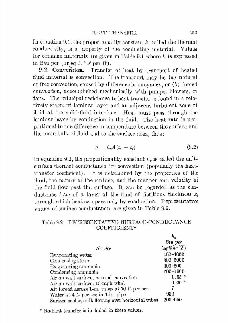
7/16/2019 Engenering Agriculture Perry
http://slidepdf.com/reader/full/engenering-agriculture-perry 222/422
HEAT TR.\NSli'ER 213
In equation 9.1, the proportionality constant Ie, raIled Lhe thpl'mul
('umlul'tiviLy, is [ I property of the condncting llluteri[LI. Values
for common materials are given in Table D.1 where k is expressedin Btu pel' (hI' sq fL of pel' ft).
<u
9.2. C o n v e ~ ' i t i ( l l l . Transfer of heat lly transport of heated
fluid material is convection. The transport may be (a) natural
or free convection, caused by difference in buoyancy, or (u) forced
convcct.ion, accolllplishcd mechanically with pump8, blowers, or
fans. The principal resi8tanrc to heat tl'allsfer is found in a relo.
tively stagnant laminar layer and an adjacent turbulent zone of
fluid at the solid-fluid interface. Hcat must pass through thelaminar layer uy conduction in the fluid. The heat rate is pro
portional to the difference in tcmperat,ure between the surface and
the main bulk of fluid and to the surface area, thus:
(9.2)
In equaLion 9.2, the proportionality constant he is called the u n i t ~surface thermal conductance for convection (popularly the heattrallsfer coefficient). I t is determined by the properties of the
fluid, the lllttUl'C of the surface', and tho ll1lUllll'l' aIlcl velocity of
the fluid flow pnst the surface. I t can be l'egarclell as the con
ductance 7';/:1:/ of a layer of the fluid of fictitious thickness XI
through which heat can pass only by conduction. Representative
values of surface conductances are given in Table 9.2.
Tahle 9,2 REIJRESENTATIVE SUHJi'ACE-CONDUCTANCECOEFFICIENTS
Evaporating Wt1terConc1emdng steam
Evapomting ammoniaConclensin!!: ammonia
Air on wall tmrface, l1lttural convectionAir on wall Rurface, 15-mph windAir forced acrOSR I-in. tubeR at 10 ft pOl' sec
Water at 4 ft pOl' sec in I-in. pipeSurface cooler, milk flowing over horizontal tubes
*Radiant tru,nsfer is included in these values.
heBtu per
(sq it h1' OF)
400-4000:300-5000:300-500900-1500
1.65 *6.00 *7
930200-650

7/16/2019 Engenering Agriculture Perry
http://slidepdf.com/reader/full/engenering-agriculture-perry 223/422
214 J\GHICULTURAL PROCESS ENGINEERING
9.3. Radiation. Radiation is the emission of energy, without
lWe([ of a concluding or cOllYccting meclium, from the surfaces of
opaque boLlies and from within semitransparent objects. Fundall1!mtally, radiant phenomena are described partly by electromag
netic wave theory aml partly by quantum thenry. A narrow band
of thermal radiation stimulates the eye and is called light. For
example, energy is transferred from the SLln to the earth by
thermal radiation. However, Uttmnal radiation is also emitted at
low temperatures, thus the lnmmn body dissipates heat partly by
radiation. Radiation Tate depends upon the area and the nature
and absolute temperature of the surface. Tho relationship ofthese factors is rldined thus:
(9.3)
The first proportionality constant, E, the emissivity, it; a property
of the surlace 01 material, tllC ratio ot its emissive pmver to that
of a pel' feet rariiator. The seeoncl, (T, the St,efan-Boltzmann con
stant, is a numerical constant for a perfect radiator, 0.173 X 10- 8
Btu pel' (hI' sq ft °R4). With this numcl'ical value, the temperature must, be given in degrees Rankine, i.e., degrees Fahrenheit
absolute or (OF + 4(i()).
CONDUCTION
The thermal conductivity of most materials is a function of the
tempera Lure. Note Table 9.1 for conductivity valucs, some of
whieh arc given at two temperatures. That of most pure metalsdecreases slightly with rise in temperature. The conductivity of
alloys is often lower than that of the principal constituents and
usually rises ,,,ith increase in temperature. For most insulating
materials, excepting magnesite refractory brick, conductivity in
creases with temperature. Whcn conductivity is linear with tem
perature, as is usually true for fairly wide ranges, the heat rate
in a plane wall can be founel correctly by llsing conductivity at
tho arithmetic mean of the temperatures of the faces.9.4. Steady-State Conduction; Plane Walls. When the
boundary temperatures have been constant long enough that tem
peratures within the systcm have ceased to change with time a
steady-state conduction condition exists. In plane walls (pre-

7/16/2019 Engenering Agriculture Perry
http://slidepdf.com/reader/full/engenering-agriculture-perry 224/422
HEAT TRANSFER 215
slIming that e d g o ~ and corners arc' negligihle or [In' protected to
pl'eY!:'nt lateral trantifcr) the flow iti ]Jcrpenrlirular to the fUDel',
so that A. tloes not vary with diRtullce through the wall. Equation
9.1 can he <Iireetly integrated }>C'tweell definite limitR to give
Examille. li'inrl the rate of hPllt flow throngh i t (·llrk partiliDIl wall in a!'old-f<torall,e plant. TIl(' wall iH 16 fl I O I l ~ , 11 ft h i ~ h , an!l 4 ill. thick. Tit!'
IpmppratnrPH of tIl(' two facl'R arc m(linl:tincrl at :n and aOF l"['s[lcctiI'ely.I n ~ p l " t i n ~ the dinH'llHiol1R al1ri I ' m l ) ( > r a t l 1 ! " p ~ illio <'<[lUll ion 11.4 :Inri the thpl"lll[li
conductivity (f1·mIl TablE' g.l) of 0.025 (morr> PI'f'(·j,ply. a mean nLiup aL Ihe
mean Ip1l11wI"lLturl' of 17°F Hhould. be uRorl),
(31 - 3)q = 0.025(1 G X!l) I = 302.4 HI u per hI"
(12 · - 0)
In composite plano walls at stC'ady state the heRc rate pCI'
blJ.uare foot through each component is rOIlfitant amI flow proceedsin series through the several materials. Equation 9.4 solwd fur
the temperature rlrop through a layer gives
(0.5)
Equation 9.5 is analogous to Ohm1r; law; the tcmpf'rature drop ir;
the product of the hrat rate and the resist.ance. I t can be seenhere, also, that resistance is the reciprocal of conductance. Simi
larly, for convective transfer, the surface resistance can be found
from equation 9.2 to be 1jh,.A. For the (lompoRite wall shown in
Fig. 9.1,'i - In = (Ii - tI ) + (II - (2) + (t2 - 13)
+ (ia - 14) + (14 - tn)
Solving for (/,
(
X4 - .Ta) (1)1+ k"A + hoA
(Ii - to)q = --------------------------
1 La LII L(" 1-+-+-+-+Ii;A k"A kbA kcA hoA
(9.6)
(9.7)
(9.8)
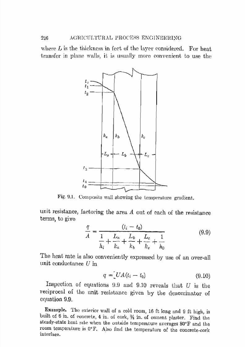
7/16/2019 Engenering Agriculture Perry
http://slidepdf.com/reader/full/engenering-agriculture-perry 225/422
2Hl AGRICULTURAL PIWC'ESS ENGINEERING
where L is the thieklless ill feet of the byer considered. For heat
trallBfer in plane walIti, it is usually more cOllvenient to use the
Fig. 9.1. CompDsite wall showing the temperature gmdient.
unit resistance, factoring the area A out of eaeh of the resistanceterms, to give
q
A
(t i - to)
1 La Lb Lc 1
- + - + - + - + ~hi ka kb lee ho
(9.9)
The heat rate ill also conveniently expressed by use of an over-allunit conductance U in
q = ' UA(ti - to) ( ~ l . l O )Inspection of equations 9.9 and 9.10 reveals that U is the
reciprocal of the unit resistance given by the denominator 01
equation 9.9.
Example. The exterior wall of a cold rOOIll, 16 it long and 9 it high, is
built of 6 in. of (,ollcl'etc, '1 in. of cork, % in. of cement plaster. Find thestcady-state heat mic when the outside temperature averages 80°F and theroom ternpemtlll'e is O°F. Also find the tempCl'l1tlll'e of the concrete-corkintGrface. .

7/16/2019 Engenering Agriculture Perry
http://slidepdf.com/reader/full/engenering-agriculture-perry 226/422
HK;\T TR AN8FER 217
From Tahle 9.1, the contiul'I i\ itif's of conen'te, ('ork, am i lllai',tpl' are 0.54,
0.025, ano 0 1 Btu pel' (hI' ~ q i t of ]lPr ft) rPH]wPli\·P]Y. From Tablf' 9.2,
Ihe outside :'urf:H'c c'onrluctancl' (for 15 llJph wind, with l'lldiant tralll,fer)is 6, and the inside :-;\1I"£:U'(' conondancp (for "still" air) is 1.65 Dtu per (hI'
sq f t of) .
Hj X (l X (80 - OJ
I j = (l t :1~ + H + TIf +I}I_+_l_G 0.54 0.025 0 . 1 l.fi5
lH X 80
O.lfi7 + O.112R + 13.333 + 0.125 + O.{jOS
= 11,1)20/15,157 = 700 Btu]wr hI'
The lemppral me drop from the' o \ 1 1 . ~ i d c to the ('01H'rpl e-rork iul l'rfal'c is
proportional to the r c ~ i , , 1 anee Clll'01111tpl'l'ti 11]1 to Ihut point. AH gi\'C'1l in
tIl(' of'Iloll1inator aho\·c, the oYl'l'-:lil resistanl'C' iR In.I57°T<' ]WI' (Btll 11<'1'
hI' aq It), while IhaL from Ihp acij:u'PIlI 80°F air 10 Ihe rl('sil'cd inll'J'
face i" 0.167 + 0,928 or 1.0(H. The tl'lllpprature at. the point is then
80 - (1.094/15.175) (80 - 0) or 74,2°F,
9.5. Steady.State Conduction, Cylinders. For conllurtinn in
cylindrical objects, it is convenient. t.o write equation D,l in eylindrical coordinates,
q = -7cA(dl/dr) (9,11)
/' being rUllius in feet..For stea,dy-state radial flow, with circular t-lymmetry and negligi
ble transfer at the ends, since 11 = 21f'rN, N being the cylinderlength in feet,
elt = -q/21f'kN dr/r (9,12)
Integrating equation 9,]2 between definite limits h und t2 and 1'1
and 1'2 respectively,
(9.13)
Equation 9.13 l'cveah, that the temperature is linear with thelogarithm of thc radius an(i that the reHisiau('e to heat flow de
pends upon the logarithm of the radius ratio and not simply upon
the thickness.
Heat £low in th<:> hollow cylinder can be expressed in a formsimilar to equation 9.4 by the use of a mean radius for finding an
equivalent area for an equivalent plane wall, thus:
21f'rmNk(t1 - t2 )q = - (9.14)
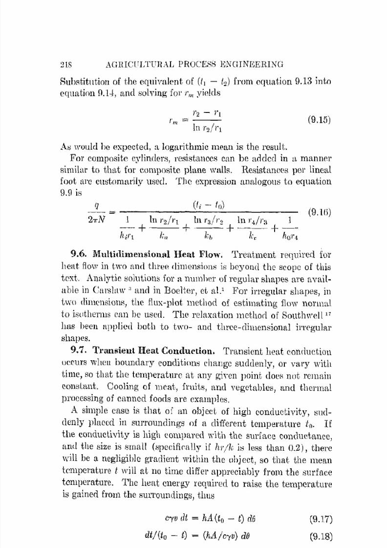
7/16/2019 Engenering Agriculture Perry
http://slidepdf.com/reader/full/engenering-agriculture-perry 227/422
2IS AGH.ICTTLTUHAL PHOCESS ENGINEERING
Substitlltioll of the equivalent of (11 - 12) from equation 9.13 into
equation n. U·, llncl solving for I'm yields
1'2 - 1'1I' =- - -ii i In 1'2/1'1
At:i wuuld he expected, a logarithmic Illflan is the result.
(9.15)
For composite cylinders, resistances can be added in a manllel'
similar to thllt for eomposite plane walls. HesistLtnees per lineal
foot nrc customarily used. The expression annJogolls to equation
9.9 is(Ii - to)
(9. Hi)
9.6. Multidimensional Heat Flow. Treatment required for
heat flow in two and three dimensions is beyond the scope of this
text. Analytic solutions for a numher of regular shapes m'e flVail
ahle in Carslaw " and in Boelter, et flU For irregular shapes, in
two dimcnsions, the flux-plot method of estimating flow normal
to isutherills can be used. The relaxation method of Southwell 11
has been applied both to two- and three-dimensional irregulnr
shapes.
9.7. Transient Heat Conduction. Transient hel1t conduction
Deems when boundary conditinns ehllllge suddenly, 01' vary with
time, so that the temperature at any giYcn point doeR not remain
cOl1sbmt. Cooling of meat, fruits, and vegetables, and thermal
processing of canned foods are examples.
A simple ease is that of an object of high conductivity, t-mc!
denly plaeud in surroundings of H different temperature to. I f
the conductivity is high compared with the surfa,ce conductance,
[tnd the size is small ( ~ p e e i f i r a l l y if hr/k is less than 0.2), there
will be a negligible gradient within the object, so that the mean
temperature t will at no time cliffeI' appreciably from the surface
temperature. The heat energy required to raisc the temperature
is gained from the surroundings, thus
c'¥V IU = hA (to - t) dO
dtj(to - t) = (hAjc')'v) dO
(9.17)
(IU8)

7/16/2019 Engenering Agriculture Perry
http://slidepdf.com/reader/full/engenering-agriculture-perry 228/422
HEAT TRANSFER.
where v = volume, cu ft.I: = specific heai, Btu per Ih of.
'¥ = specific weight, Ih pCI' Cll ft.e = time, hI',
219
~ W h e r e the thermal propprt,jes do noi change with temperature und
the 8U1'l'IHlIlfli.ng tempcrature is ('ollstani, ('([nation \).18 cnn he
readily integmtrd. Using thr lowE'r limits of t = it , ..·hf'n e = 0and the upper inclefinit(, limit. of t = t when () = () in orclN to find
th(' variation of t with tinw,
ot'
/-/0 -hAIn--- = - - ( )11 - io c'¥V
t - to-h , t /I
C)V
- - -= eII - to
(g.19a)
(9.l9b)
Example. Fmd lIIP \PDlpE'mtlll'r of a R\eP[ bul', 3 in. il l d Jail H' ICl' and12 in. lung, initllllly al 70°F, 40 min aftf'l' }JPIllIl; su<irlc'uly plal'l'([ in an
aun('alinll; [Ill'UaCl' whelP Ihc tf'Il1Pf'wj]]],c 6000 P, j f til(' ~ \ l l ' f U f ' e tlwnnal
('Ulll\tH'ltlllf'e e ~ t i m l l . l ( ' d to bc' 6 Bllll'C'1' (Ill' fI, of) . TIll' Rjw(,lf ir healof sLeel j" 0.12 Bill [lPl' 111 OF, Ihp ~ p C ' f · i t i e \wil1.h\ '150 Ih pC'l' ell ft, llnd tllp
thc'l'lllal ('onrlUl'tivlty 26 Btu !,PI' (hI' H(! i t OF 1'('1' fL).
First, tiutf'l'llllIl(' WI10lhf'1' til(' lelIll'('ratlll'(' Will be 1'l'llrlily riisillbutf'([ wltlnll
t hl' bar, by ('oll1]mtiJl!!: Ihe l'l'latiVl' ~ l l l ' f : l ( ' f ' - i l l i ('lllal rcc,istan('u erit Pl'iOll
hr/k. This 6 X (¥,.,)/2() or 00211, wltidl I' wl'll helow the ll\aXim1ll1l allow
abll' VUhlP of 0.2 gi \ en al)()\·p.
Thf' SIlrJ"Ul'(' mca, P11(lH ]llus cylindrim[ ,ide',,", j , 0.R83 SC J ft.. TIlf' \'ohlln('
0.049 ( ' l l [t. E(l\lttttoll 920 IIlf'11 gins
t-fOO _ ox .HS:JY (40/60)_l_ = C o12XI50XO.Il-!<)
70-(iOO
= 1,-1.33 = 0.202
t = GOO + 0.2G(70 - GOO)
= 4(il OF
Where the :·;urfa<'u eon<luetnnce IS high with l'etlpect to the
thenmd rOlllluetivity of nn object. to he heated or ('ooled, the
l'mrf'acc temperature chnngei:l faster than t.he interim, and equation
9.Hlb docs not. apply. It is n e ( ' t ' s ~ a r y to consider local changE'S in
temperature with time, which resulL from differences in tempera
ture gradients. For transient heat flow, in one direction, an in
stantaneous heat balance gives

7/16/2019 Engenering Agriculture Perry
http://slidepdf.com/reader/full/engenering-agriculture-perry 229/422
220 AGRICULTURAL PROCESS ENGINEERING
iJl (iJlj iJ;r)Cr d.l: ely dz - = k dy dz-- d:r (9.20)
iJ8 iJx
Where thermal properties are constant with time, temperature,
and position, this becomes
or-I...... ., ::
1.0
0.8
0.6
0.4
0.2
0.1
O.B
0.6
~ 0"'I 0.4I i
:
0.2
0.10.8
0.6
0.2
(9.21)
'\ ' ~,\\'\:: :--.:: r-..,- ::- - r-. 10.0---\\\ ,"........ ~ ~ - - . - ~
-
\ \ '\." ,,,", i'.... r---. r-...
-I--. 6.0
-:::-
\ \ '\ "'-'I'-. ~ ............. - .l " - I - 4.0_:--
\ ' \ \ ~ ~ ~ " , "-3,0 ___
--.0 -\\\ L\ "'df;i.o,
1.5 "- ~ ...........r--........
o 0.25 0.5\ -" ' "
"'".......i'---- ..............
;\[\ '":O \ ~
'"
,Center
"~
." -...,\. ~ r-..
10.0 ........\ " I"-.....l\ \ "- I'" ~\\ \ \ , .................\' \ " "
-.... ~\\ 1\ ~ 5 0 ~ 1 . 0 2.0 ......... ~
r--......
1\0.10 6.25 .1\
""""
~-.........\ ~
1\ I\.Average ~
~ ' " ~ -.....;:: r--. - r-.~ :--... :--...... - -t - - -I - - 10.0:: ~\ . . "'- ::--.._ r--- I- - - 6 . 0 -
\ f\.'\. ,,,,- ......... ................. r-- r-- -r-- 4.0
\ ' \.'"......, ............. - - 3 . 0
-__r--....
----\ 1\ .'\"""" '" ....... 2.0 ......... ----.0
1'1.5 ::--........
: ~ 0 2 { ~ T I ' "'"....... ........,
~'"
~'--r--........."- J'.... Surface
0,2 0,4 0.6 0.8 1.0 1.2 1.4k 0
c:y r02
Fig. 9.2. Transient. t()mperat.ures in t1 sphcrc.
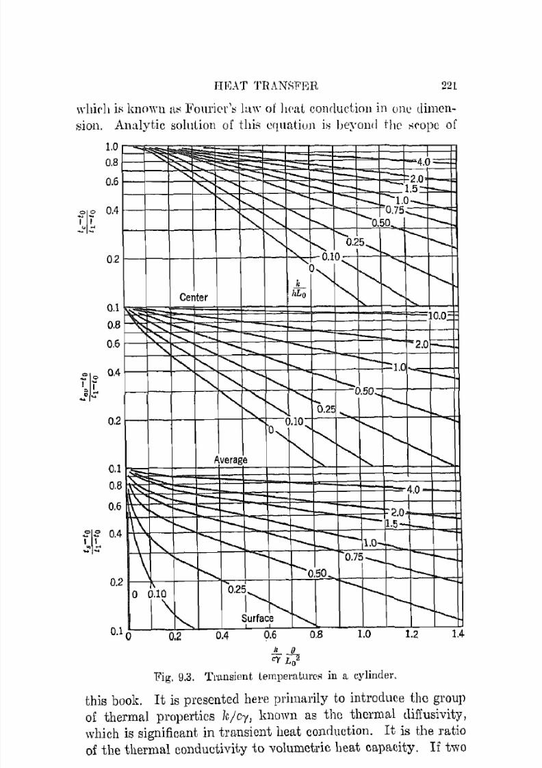
7/16/2019 Engenering Agriculture Perry
http://slidepdf.com/reader/full/engenering-agriculture-perry 230/422
H I I ~ A T TRANSFER 221
which if-; known [It-: F o n r i ( ' r ' ~ law of hr'ut eOllciuetioll in one dimen
sion. Analytic solution of thiR e(llwtion iH beyond the :o;('opc of
1 . 0 ~ ~ ~ i i i i ~ ~- . . ; : ~ ~ R' - - ' 4 . 0=.8
0.6
°1°0.4
I j'_t..o,:::
0.2
Center0.1
0.8
0.6
2r0.4
I -
"
-- 0.2
0.1
0.8 4 . 0 - t - -
0.6 - t - - - I- . 2 o,+--...I.=-+t--..... -I-- 1.5'- -
°1° 0.4I '~ : : r-- - t - -t--\-.... 1.0-,....,
0.2
0.2 0.4 0.6 0.8 1.0 1.2 1.4
k 0ryI7
Fig. 9.3. Transient tempel'aturcil in a cylinder.
this book. I t is presented here primarily to introduce the group
of thermal properties leJer, known as the thermal tliffusivity,
which is significant in transient heat conduction. It is the ratioof the thermal conductivity to volumetric heat capacity. I f two

7/16/2019 Engenering Agriculture Perry
http://slidepdf.com/reader/full/engenering-agriculture-perry 231/422
222 AC!IUCULTURAL PHOC'ESi-\ ENGINElijRING
oJ,jceb of till' saltle size and sall1e thermal diffusivity arc placcd
in the Raine surroundings, they will expcrience the same yariations
1.0
0.8
0.6
°1°0.4
I,.....«J.:::
0.2
0.1
'" -'""' ..... :--. h. r- - 1 0 . 0 ~' \ :-.......: ....... i- F::: =1--- - 6.0=
" \: ""-,-......
I-.... r---. -I-- -- 4.0::::::
\ ~ '-... r---.. r--..........r--- ........-- 3.0;;;;;:::
\ "\"'- ['.._ ...........
............................ 2.0 t - -"-
1\
'" '".........
j'-....I'-..1.5;;;::::
r--~ .....1.0
'\ "- ....... 0.75 '-.... ........ I'---.0 . 2 \
0.50,I'---.
0\
'"........__
Center hro I\.. ~0.8
0.6
~ ~10.0 ="'"
;;::;::
1\ ' - ........ - f---
\ "\. ~ .......... --°1°
0.4
I i~ g ~
0.2
0.1
\1\ ' "'........
I--.... F '2 .0 ....
1\\
'".......
I'....
'"- t - - :--........
'\ \ '" ""1.0 .......
r........1\ 6.25 0.50 ... ............
I'---.,0 .1\ ~ i'--t'-...
I'---.I'---.verage 1\ r\.
0.8\ \ " f . . . _ 10.0
0.61\\ ;:-;;;:: f': - - i - . -I - - 1-6.0-\" .......... J"....
-_ 1 -- r-- - t-4.0 i - .
°1°0.4
II
0.2
\" I ':.............. .............. t--f..._ t - - t- . - 3 . 0 -
r -"""I
t'-... 1"'" ........
r........ r--. r--....... - 2 . 0 - r -
1\ f'........ ' ~ ............ 1.5-1-- -- -
1--1.0 r -'-.. I--.... t--.....
0 0 . 2 ~ .......r-.. 0.75 r-.......
............
'"
0.50 i'-- r-.......I'---.urface ~ )'...... r.......
0.2 0.4 0.6 0.8 1.0 1.2 1.4k 0
C')' r02
Fig. 904. Transient tcmpNatl1l'eS in a slab.
in temperature. The thermal diffusivity thus appears in one of
the dimensionless moduli for transient heat flow, the Fourier number, 01' (kjcy) (Ojr2).
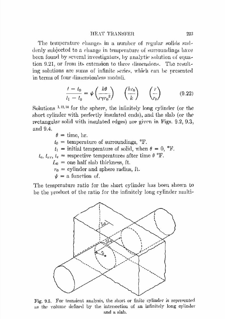
7/16/2019 Engenering Agriculture Perry
http://slidepdf.com/reader/full/engenering-agriculture-perry 232/422
IIIUT TH.\'NtlFEH 223
The temperature f'hang,e:-, in a number of J't·g,ular solid:; s l l f l ~denly l:Hlbjected to a rlmng,e in telllprmturc uf ~ t l l T O l l I H l i 1 1 g ; ; hav(;l
beon found. by seveml investigaturs, hy nnalyti(' holution of e q u a ~tion 9.21, or frol1l it" extension to three di1l1011,;ion:;. The r e ~ u I L in!); solutions are Rums of infinite ~ e r i e ~ , whif'\l can be presented
in terms of foul' ( 1 i m e m ~ i o I l l e S f i morlnli.
1 -10 ( k() )
[1 - to = tf; C"{I'02 C ~ o ) ( ~ ) (9.22)
Rolutions 1,12, J.I for the sphel'<', the infinitely long eylinder (or the
short cylinder with perfpctly insulated ends), and the slab (or the
rectangular solid with immlated edgeR) are g,ivrn in Figs. \).2, O,3,
and 9,{,
0= time, hI',
to = temperature of surroundings, of.
t! = initial temperature of Holicl, whon 0 = 0, °F.
le, tay , t" = respective temperature,; after time () of.
Lo = one half slab thickness, ft.
1'0 = cylinder and sphere radius, ft.t/! = a function of.
The temperature ratio for the ",hart cylinder has bcen shown to
be the product of the ratio for the infinitely long cylinder lllulti-
Fig. 9.5. For t r > l l l ~ i e l l t a l l u l y s i ~ , thc short or finitc cylintlpl' is l'cl1rcf'cnted
us tho volume Uefillf'd by the intcrsection of all infinitely IOllg cylinderand a slab.

7/16/2019 Engenering Agriculture Perry
http://slidepdf.com/reader/full/engenering-agriculture-perry 233/422
224 AGRICULTUHAL PROCESS ENGINEEIUNG
plied by the ratio for the infinite slab of a thickness that defines
the length of the short cylinder, Fig. 9'[). Similarly, the ratio for
n rectangular solid ,vith all surfaces exposed is the product ofthe ratios for three slabs of thicknesses equal respectively to the
three dimensions of the solid.
Example. A number 2 can, uet diameter 3 ~ i f l in., net length Hill in.,
~ ( ) n t [ l i n s 1.25 Ib of 11 solid-pank food product which has a moisture content
of 80 per cent and a specific w(Jip;ht of 6S Ib pf'r eu ft. The cnn, with its
contents initially at 180°]', is suddenly ] 1 h l U ( ~ r l in a retort where the SUl'
rmllHling temperature is prolllpLly rai;;ecl to 240°F with steam. li'ind the
temperatUl'8 at the center of the can at. the pnd of 30 min. Smface con
dnetanee h for condensing sLeam, lOOO Btu pel' hr-ft2 °1".
The specifie helLt is estimated to he 0.84 Btu per I)) OF; thc tlwrmal COIl
cluctidty, 0.25 Btu pCI' (hr sq it of per ft). The thermal diffusiviLy is then
0.25/(0.8'1 X 68) or 0.00438 sq fL l'pr hr. The radius is (3''Yiu)/24 or 0.138 ft.
TIll" half thiclmcss of the plmlf! Hlnb which defines the length iR (4%G)/24
or 0.17<1 ft .I·'ol' the cylinder
k/h1'O = 0.25/(1000 X 0.138) = 0.0018At 30 min
kB/c,I'02 = (0.00:138 X 0.5)/0.1382 = 0.115
From Fig. 9.3, the residual temperature ratio is 0.8 at the center.
For the Hlab
k/hLo = 0.25/(1000 X 0.174) = O.OOHAJ, 30 min
kB/c,Lo2 = (0.00438 X 0.5)/0.1742 = 0.0725
From Fig. 9.4, the residual temperature ratio is OJ)5 at the center.
For the short cylinder, the residual temperature ratio is the product of the
ratio for the long cylinder and the slab which defines the ends.
From this
t - to-- = (l.S X 0.95 = O.7()II - to
t - 240180 _ 240 = 0.71)
t "" 240 + (180 - 240) X 0.76
= 240 - 45.6 = H14.4°F
Analytic solutions are not readily available for many problems
that involve irregular initial temperature distribution or in which
boundary eonditions are not com;tant or where properties ehangewith time, temperatul'e, or position. In some such cases, numeri
cal methods 0,6,17 of solution can be used, or devices for solving
analogous electrical problems may be available.
7/16/2019 Engenering Agriculture Perry
http://slidepdf.com/reader/full/engenering-agriculture-perry 234/422
HEAT T R A ~ R F l m 22ii
CONVECTION
Two principal k i n d ~ of problems arise in cOlwurtion. AR illCli
('aLed by equation 9.2, Lhe burface thermal ('onclurtance he llnd
the Lelllperatnre difference must both be estahlished. This sec
tion will treat the estimation of conductancc's and a later :sed-ion
on heat exchangen; will (leal with trmperatllre (liffprPIlr'c:o:.
11uch of the rCAistance Lo lIt'at transfer by r'onvpction is found
in the layrl' of fluid, in laminar flow without mixing, moving arl
jaeent to Lbo surface. Heat is transferred through this layer onlyhy conduction. The surface crmdudance can he thonght of (1 "
the conductance uf a fictitious layer J.'[, having the conrlut'tivity
of the fluid, (lefined by h,. = "/1'/. The eonductanre can be in
creased by l'('ducing the thickness of the laminar layer by more
vigorous agitation, more actin thermal circulation, or by opera
tion at higher Hcynolcls-nlllUbpl' values.
Although the roncrpt of the ficLitioUf; equivalent layer is helpful
in pip-turing convection resisLance, it iA not necessary to determinethe t h i c k n e ~ s ill convection calculations. A more direct approach
is to establish conditions that gi,'e similar patterns of fluid flow,
for which similar temperature patterns result, As would be ex
pected, the ReynolrlR number Re (TW Y/ fh or DO/p.) whieh is a
criterion for similarity of fluid flow if> a valid rritel'ion in forced
convection tr[tn:-;fer. For natural or free convection transfer, a
criterion that relatrs t hr bunyaney forct's tending to promote fluid
transport to the viscous and inertia flow resistames is required.Suuh a ('ritel'ioll (D:J y2o{3 Aflp,2) has been named the Grashof
number, GI'.
For convection, a lllociulus that will include the thermal con
ductanre is ohvioui:lly required. The criterion (hD/k), nHmed
N1i fo1' Nm::;dt, ha::; heen founcl valid. Since this ean be written
a" D/(k/h,.) = Dj:rf, it can be th()ught of as the ratio of a perti
nent sig11ificant physical climen8iul1, :mch as the diameter of a
pipe, to the fietitious layer thickness. The influence of thethermal properties is included hy the modulus (c}L/k) whieh is
designated the Prandtl number, Pl'. In systems where the flow
pattern changes from point to point, as it does neal' tho entrance
of a pipe, a relative-position modulus such as (LID) is required.
7/16/2019 Engenering Agriculture Perry
http://slidepdf.com/reader/full/engenering-agriculture-perry 235/422
226 AGmCLTLTURAL PROCESS E N G I N J l ~ E R I N GFur fTC0 rOll"cebon, the general exprcssion is then
(9.2:1)
For fowed convect.ion, the general exprCHl-liOll is
(9.24)
The functions "'" and "'1 for natural and for fmeed convectionhave bccn determined experimentally for lllany HystemK in COlll
mercial and industrial use. In SOllle eases where they are not
simple fUllctions, approximate power functions are usee! over
slleeified rang'es of the yarinblcs.
9.8. Free Convection. For fTeE eonwetion about horizontl11
('ylinrlers, equation !l23 can be representee! by a power function.
hD
= cD 3 ' Y ~ : { 3 fJ./. DJ.I,Jn
k fJ.- k (9.25)
Over the range of 101 < Or·PI' < 10 9
, C = 0.53, n = 0.25. AboveGr·PI' of 109
, C = 0.12 and n = J ;{.
9.9. Free Convection, Gases. For gases it is convenient to
solve e<1uation 9.25 for h and then to grollp the constnnts and
thermal properties as follows, for the lower range,
[ 'Y2g(3clc:JjOo25(l::..t)O.25 (I::..t)D .25h = 0.53 -_ - = b -{L D D
(9.2())
The coefficient b is a particular function of temperature for each
gas and includes the effect of temperature upon the thermal prop
erties. For air, b = 0.288(1 - 0.000570. Since b varies only
slightly with air temperature at normal temperatures, it is COIl
venient to use a mean value of 0.27. For air, the equation then
becomes
h = 0.27 (I::..tjD)O.25 (9.27)
For shapes other than horizontal cylinders, equations similar to
equation 9.25 are available, but with constants appropriate for
the particular shape, a steam radiator, for example, or a bank oftubes.
7/16/2019 Engenering Agriculture Perry
http://slidepdf.com/reader/full/engenering-agriculture-perry 236/422
H T ~ A T TRAl'iSFER 227
For plane surfn,ces in air:
1. Horizontal, heated facing upward, 01' cuolNI faeing down
ward, over :3 ft square,
II = 0.38 ( ~ t ) O . 2 . J (9.28)
2. Horizontal, heated facing (lowl1wanl, ()J" coolerl facing up
ward, over 3 ft, RC[lU1re,
II = 0.2 ( ~ t ; n · 2 r ; (0.2\1)
3. Vertical surfaces over 1 ft high
h = 0.27 ( ~ t ) n . 2 5 (n.30)
4. Vertical air spaces, over 1 ft high and more than 1 in. \vide.
Equation 9.30 call hE' applied, on recognizing that two resistances
occur in series, with half the ovrr-all Hurface-to-tmrfac(l difference
available for each. TllUl-l
o27 ( ~ t ) O . 2 5h = ~ " 2 = ( ) . 1 2 ( ~ t ) ( ) · 2 5 (9.31)
For vertical spaces less than 17f in. wide, cOllvection is 1'e
stricterl, being almost SUpPl'l'ssecl in ~ ] 1 a c e t : l less than }::l in. wide.
Conrluctnnces for airspaces from to 1% ill. wiele, l'e)lorted by
Rowley and Algl'en,' include the radiation whirl! occurs in paral
lel with the conveetioll.
Example. FilH[ the ral(, of h('at l o ~ ~ pel' liuf'al foo!' frolll I t 2-in. bare
horizontul stpam]Jipf', with a Surfl\l 'C tell1!lpmtl1I"(, o f 330°F, in It 1"00111 at70°F. The outRide dialllPtCl' of 2 in. JlolUiJlnl ]lipe 2.38 in.
' rhe tPlllllPl"lltUl'e difference 330 - 70 or 260°F. The Qut:<ide cliallwll'!"
iH 0.H18 ft. Equntion 9.27 tholl g i v p ~
h = 0.27(260/0.HJ8)0.25 = 1.02 Btu pt 'l ' (hI' Rq ft °F)
The 10RB mte P(,I" linC'lIl foot, by ('qlll1tioll \1.2 (for r'onv('ct,jon only),
q = Ul2 X 0.1118 X 1l"(380 - 70) = 2tl3 Btu pl'l" hI' ft.
9.10. Free Convection, Liquids. For liquiclt:l the coefficients
uf thermal expansion and viscosity ehange markedly with tem
pentture. An eXllret:lsion similar to cquation 9.27 is of doubtful
utility because the limits within which it is applicable are not
readily recognized. Instead, equation 9.25 is rewritten

7/16/2019 Engenering Agriculture Perry
http://slidepdf.com/reader/full/engenering-agriculture-perry 237/422
228 AGHICULTURAL PROCESS ENGINEERING
hD/1;; = C(aD 3 /::"t)" (9.32)
in which it can be seen that
a = "'./g{3c/)J.lc (9.33)
Tabular values of a for particular temperatures for a given fluid
can be computed. From these, an approximate algebraic repre
sentation may be developed. FOl' water, between 50° and 180°F,
(9.33a)
in which tt is the mcall temperature of the laminar layer, midway
between the surface and bulk fluid temperatures. The constants
!Inri exponents in this expression have no special physical signifi
cance but are simply tl convenient way of Humm,uizing data on
water.
Since watcr has 11 maximUlll density at 39°F, equations 9.32
and 9.33 cannot be used for temperature differences which span
39°F. ~ W h e r e it is desired to cool quantities of water with ice,
temperatures below 39°F arc not readily sccured with ice floating
in a tank. As water adjacent to the ice begins to cool below39°F, it tends to remain at the top of the tank, with very poor
eonvection transfer of its heat to the ice. A more effective ar
rangement is a spray or shower of recirculated water over cakes
of ice supported above the wnter level on a screen rack.
Example. Find thr> h""t-tl'ansfr>l' coeffirienL fmm [1 3-in. dirulletel' ste\Lm
pipe, with !t surface of 210°F, to water in [1 water-heat.er tank at 150°F.
The outside diameter of 3-in. nominal size pille iH 3.5 in. or 0.292 ft.
Equation 9.33 can be med, with "'tlues for water from equation 9.3311.T I H ~ mean film temperature is (210 + 150) /2 or 180°F. From equation
n.3311, (I = 6.3 X 10⁴ (180 - 1Oj:! or 18.2 X lOS. In equation 9.25, the group
in the bracket, whic:h is the Grashof-Pmudtl 1111Inber product is 18.2 X 10 8 X0.292 3 (210 - 150) or 2.72 X 100. Sinee this is larger than 100, the value
of C (equation 9.25) is 0.12 and n i s ~ . Thus
hD/k = 0.12(2.72 X 10⁹) ' ; = 0.12 X 1305 = 1(\7
!LutI, sinee k for watcr = 0.38!) at 180°F,
h = 0.38H X 1G7/0.292 01' 223 Btu per (hI' sq ft OF)
9.11. ConVec.tioll Transfer in Boiling. When heating SUl'
faces are at temperatures above the boiling points of the liquids
in which they are submerged, much greater heat transfer will
occur than predicted from equation 9.25, because of the violent

7/16/2019 Engenering Agriculture Perry
http://slidepdf.com/reader/full/engenering-agriculture-perry 238/422
HK\T TRAK;4FER 22fJ
agitation resulting from I:)urfare hoiling. The ('ondudt1D('e>i vary
greatly with the arrangement, nature, and ('oncliliull of the I 'UI'
face. Very roughly, for wate]', for i!:..llcRf' than-tO
h == 100 (ill) (9.34)
At telllPcrature differellce::; g,reatcr than -lO°F, vapot' formatiull
becoltles HO rapid that vapor bl::mkding of the surface O(,Clll'R,
and g,reater cliffcrenet's give no greatcr transfer. There may be
(langer of sevC'rely overhenting the surfac(' of direct-fired vessels.
For organie liquids, the boiling ('omluei.ance may he only y, 0 to
~ ~ that for water.
9.12. Surface Condensation of Vapors. In tl'l1nsfer of heat
from condensing 'laporR to condenser i:>nl'faces, the principal re
sistance exists in tIle film of condensed liquicl adhering and drain
ing slowly from the surface. The recollllllcndcli value for con
densing steam is h = 1000. With particular care to obtain drop
wiRe condensation insteacl of film condensation, valuos as brge as
6000 have beon secured. For organic vapors, a conservative value
is 200.
Air or other llollconcknsahle gas which may enter with the
vapor will tend to be concentrated at the vapor-romlensate inter
face, ancl offer substantial resistance to eondensatiun. Steam jet
ejector;; or dry-vacuum pumps are used to remove noncolldensable
gas from fmrface or jet condensers. Nonrondensable gas purgers
are installed on large ammonia refrigeration f;;ystems.
FORCED CONVECTION
Forced convection is employed in two general types of systems,
(a) fluids flowing in pipes of circular or annular cross section, anll
(u) fluids flowing across single pipes, or finne(l tuhes, and other
flat or irregular objeettl. The general NusJ:lelt equation, 9.24, can,
with appropriate constants, be adapted to each.
9.13. Forced Convection Imide Pipes. For heat transfer in
long pipes, a single power function has been found arlequate.Since turbulencc is well developcd by the cntrance conditions in
much industrial apparatus and only mean values over the length
of the pipe are desired, the (L/D) group is usually omitted.
(9,35)

7/16/2019 Engenering Agriculture Perry
http://slidepdf.com/reader/full/engenering-agriculture-perry 239/422
280 AGHICFLTUIL\.L PROCESS ENGINElmING
j" rccomlllCndcd hy McAdams for fluids of viscosities not morc
than twice that of water. Tlw Ecynolds number must be above
:.nOO to int'UJ"e turbulent flow. In equation 9.35, the thermal prop
erties arc to be evnJuntcd at the bulk mean temperature. vVith
liquirls that have a significant change in viscosity with tempem
ture, the laminltl' layer will he warmer and less viscous than the
hulk of the fl uid in heating, and ('older ant! more ViBCOllS in cool
ing. Dit tus and Boelter recognized this by using a constant of
0.0243 and an exponent of 0.4 for the Prandtl Ilmnber for heating,
and a constant of 0.02(15 with a Prandtl exponent of 0.3 for cool
ing. However, McAdams 1" prefers insteacl the single equationof Sieder and Tate 1" for fluids of high viscosity
ltD (iL)O.14 (DG)O.S (eJ.l.));'- = 0.02, - - -k iLs J.l. k
(9.3())
In equation 9.36, the fluid propcrties are evaluated at the bulk
mean temperature, except /L"' which is found at the temperature of
the surface.For a particular fluid, application of equation 9.35 or 9.36 can
be simplified hy solving for h, with the thermal properties anc!
constants grouped together and expressed as a function of tem
perature. For d e ~ i g n calculations, it is desirable to give diamcter
in inehes, D = D' 12, and to use the flow rate in pounds pCI' hour
per tube, w = G1T (D') 2/576, instead of the unit mass velocity G.
Equation 9.35 is rewritten as
(9.37)
(9.38)
in which j, defined by the constants and properties in the bracket,
is a function of temperature. When values of j for Heveral repre
sentative temperatures are plotted against t, a very nearly linear
relation is found. For water, between 40 and 210°F
f == 0.53(1 + O.OIt)
For pipes of nOfwireular eross sectirm, equation 9.35 or 9.36 can
be employed, using for D the diameter equivalent to the hydraulic
radius, Dc == 4rbYdr. With annular spaces, De = D2 - D 1.
7/16/2019 Engenering Agriculture Perry
http://slidepdf.com/reader/full/engenering-agriculture-perry 240/422
231
I f flow iH in Lhe :,;treallliinc region (Heynold:-; llUmJw]' lc;,:-; thall
2100), no lateral mixing o c e U l ' ~ , and hertt l l l l l ;:,t be transfcl'r!'(l cn
tin'ly by conduction through lalllillltr layt'I'H. Tl't'atment of thb
region and the transition region (up t(l HeYl101db 111lll1hcr of ·1000 I
iH somewhat more involYC'd than for the turhulent flow and j:-, be
yond the scope of this text. I t is treaiA'rl in detail by McA(lamH.'"
:Since heat-transfer coeffi(·ients are poor in these regiuns, de:-.ign
and operating cllnrlitiol1ti Hhould be arranged to give t urbul('llt
flow.
Example. ERt imate the ourface thrl"lnai l'Oudnd,mf'P fOl hPfl1 iug "roughbroken" t0111l1to pulp fr0111 70° to 170011', I t t thl' ral f' of 30,000 III Jl( '] ' hI' in
a tube' 2.33 in. in i n ~ i d e dilllUdE'l'. Tllf' tuhe ~ U r f l j ( ' P temp('ratllr(' "'ill I>f'
220°F. ThprInal properLies arE':
Density, 64 Ib prj' ell ft,.
Solid" content, 6 pc]' (·pnt.
ERhmated specific hraL. 0.95 Btu ppr Ib of.
V H ' ; C O ~ l t y , 3.5 centipobe at. 68°1<'.
1.9 c r n t i p o i ~ e at 135°F.
1.3 crutipoisp at 200°F.
Thrl'mal conduetivity, estinHLjpd at \)5 pCI' l'Pllt of that of water. The
hulk mean LempPl'atl11'P IH (70 + 170)/2 or 120°1<'. At t h i ~ tt'lllpprat111'P, the
\ ' i ~ r o b i t y , interpobted from the data, iR 2.15 e Q n t i p o i ~ e R , whil'h i" eqnal to
2.42 X 2.15 or 5.2 Ib pel' (hI' fl). The tlHC'rnllll t'onductivJty. at 120, I'
0.95 X 0.368 or 0.35 Btu 1)('1' (hI' HC] ft OF PPI' ft). Pipe' CI'Obb ~ e d i o l l0.1942 X 0.7854, or 0.0296 Sf! n.
Since the v i ~ c o s i t y is more 1han twh'p that of wllter, f'C[UatlOll 9.36 will
be useu. Th(' m a s ~ velocity () is 30.000/0.0296 = 1.013 X Ion lb per (hI'
ft,). The Rcynolds number iR 0.194 X 1.013 X 106/52 = 37,800, whi('h iswell into the turbulcnt zone. The' Pranclt.lnumbpl' is 0.95 X .'5.2/0.35 = 14.1.
Thc viscosity [tt, the :'!Ul'fa('c tempemtul'c of 220"1<', estimated hy extrapolu
ion, is 1.2 centipoises, or 2.42 X 1.2 = 2.\l Ih l)el' (ilr it). In!';crtiug llll!s,'
values in equution 9.36 gives
hD = 0.027 ( ~ ~ ) l ) 11(37,80W R ( 1 4 . 1 ) ~ ; lIe 2.9
= 324
Frum t h i ~ ,h = 324 X 0.35/0.194 = 585 Btu pCI' (hI' SC] ft OF)
Bpfol'l' pJ'ocppding with a full-scale design, it would be n d v i ~ l 1 b l e to ascertainby illbomtory tests at the samc Reynolds number and tllbe-Rurface tem
pFrature, whether auy signifieant reductiun in conductance will occur be
causo of accumulation of "cooked" film on tube surfaces.
7/16/2019 Engenering Agriculture Perry
http://slidepdf.com/reader/full/engenering-agriculture-perry 241/422
232 ..\CHlCUl/rUHAL PEOCESS "Kl'i'GINEERING
9.14. Forced ~ o n v e c t i o n Across Pilles, Banks of Pipes, and
Plates. For forced C'onvection across single cylinders and banks
of tubes, equation 9.24 cannot he represented by [ t single power
function for the whole range of H.eynolcls munucrs for ,vhieh data
are ltvnilable. It mny be well to remnrk here that the Reynolds
number for flow across cylinders, being based on the outside
diameter of the eylinder and the mass velocity in the free cross
section, has no direct relation to thc Reynolds number for flow in
pipes. Laminar flow may prevail from the leading edge to the
diameter normal to the flow, and a turbulent wake occurs even
at low Reynolds numbers. The numerical value of 2100, whieh isthe lower limit for turbulent flow in pipes, has no particular sig
nificance here.
9.15. Forced Convection Across Single Cylinders. For
gases flowing normal to single cylindcrs,12 in the range of
Reynolds numbers from 0.1 to 1000
hDo )0.:1 (DoG)0.52- - = 0.35 + 0.47 -
k e}.L }.L
(9.39)
While from Reynolds numbers of 1000 to 50,000
hD o (k)O.3 = 0.26 (DoG)O.flk e}.L }.L
(9.40)
For liquids flowing normal to single cylinders, in the range of
Reynolds numbers from 0.1 to 200, the curve has the form of
equation 9.40, but with a constant of 0.86 and an exponent of
0.43. Above Reynolds nllmbel'S of 200, equation 9.39 is recom
mended. In each of these equations, the fluid properties arc to
be evaluated at the film temperature, the arithmetic average of
surfnce and bulk mean fluid temperatures.
For spheres, in the range of Reynolds numbers from 20 to
1.50,000, the equation is similar to equation 9.40, but the constant
is 0.36.
9.16. Forced COllvection Across Banks of Tuhes. Banks of
tubes can be represented by equations similar to equation 9.40.The mass velocity G, to be used is the rate of flow, divided by the
minimum free area, whether it occurs in transverse or diagonal
spacing. In a bank of in-line tubes, the second row has been
shown to have a lower conductance than the first and the subse-
7/16/2019 Engenering Agriculture Perry
http://slidepdf.com/reader/full/engenering-agriculture-perry 242/422
HEAT 'l'RA NSJi'ER 233
quent rows. In u bank of :;Luggered tube:;, the second and thil'll
tubes may he from 3 1,0 20 per cellI, highcr than the fir:::t, de
pending upou the bpacing. However, the prel>:ml'e drop for stag
gered tubes is higher than that for in-linc tubes.
·With factory-assclllhlccl finned tubes, particular ('onstants for
an assembly are doterlllillPll hy test. Expre"sions such a:-; equation
9.40 aiel in correlating the Ilata.
9.17. Force(l Convection, Plane Surfaces. Where a fluid
flows parallel to u plane surface unconfined by the walls of 1I
d u c t " ~ the flow pnttc"1'll is at first cOlll:iiderably infilleneecl by the
nature of Lhe leading edge. The distance from the leading edgeiH the significant dimension to be used in the Nus:;elt and Reynolds
numbers. A laminar layer develop:; at the learling cdge if it is
gently rounded. A turbulent zone may start at a blunt leading
edge, or it may not develop till Reynolds numbers of 100,000 to
500,000 are reached following a gently rounded eligo. The surface
conduetan('c is high where the laminar layer is initially thin,
drops as the layer thickens, rises in tho transition zone, and then
gradually drops. For mean values of the tlll'rmal l'oIllluctanee,Jakob 10 gives an equation similar to equation 9.35, hut with a
constant of 0.031, for Reynolds numbers above 200,000.
Very eareful measurcments were made by Howley, et rd.,' of
surface thcrmal condnctances for ail' flowing in a 6-by-12-in. dud
parallel to surfaces of several typical huilding m a t e r i a l ~ . The
results are cxpres:,;ec] simply as
hc+, = 1.5 + 0.1 64.Y for glassand smooth paint (9.41)
hc+r = 1.8 + 0.168V for smooth plaster (9.42)
hr+r = 2 + 0.218V for concrete (9.43)
h"+r = 2 + 0.31 Y for stucco (!J.44 )
In these equations, the SUbscript of h dcnotes that it is for COlll
bined convection and rudiatiou. l ' it; in feet per t;econd. The
values given are for n mean temperature (arithmetic mcan of
surface and its expose<l surroun<lings) of 20°F, representative of
uutdoor winter conrlitions in cold climates, at which the radiation
conductance is 0.7. SubtracLing 0.7 give8 convection conduc
tances. Since Lhe net values for zero velocity must be for free
convection (at about 45 degrees temperature difference) the
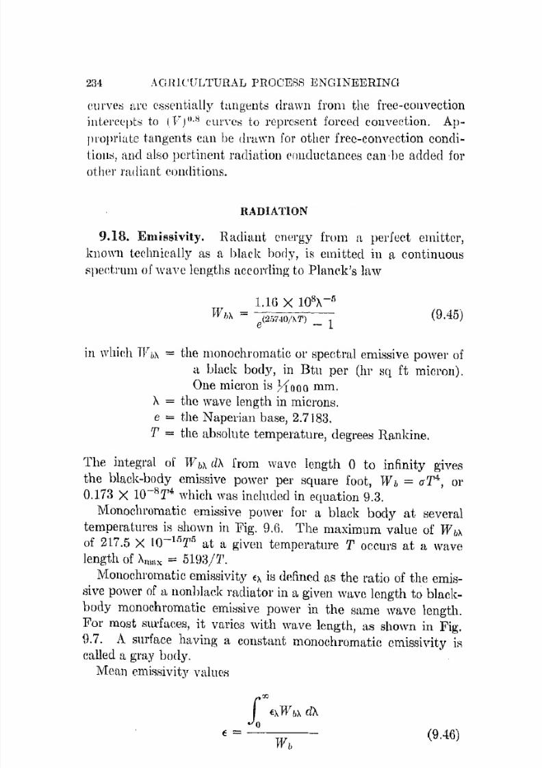
7/16/2019 Engenering Agriculture Perry
http://slidepdf.com/reader/full/engenering-agriculture-perry 243/422
234 AGHH'LTLTUHAL PROCESS ENGINEERING
curve" aru c s ~ ( ' n t i a l 1 y tangents drawn from the free-couvection
in Lel'C'epts to iT") II.H Clll'YCS to l'eprc'scnt forced cOllvection. Ap
propriate tangents can be drawn for other free-convection eoncli
liou", and also pertinent radiation C'llllductanccs ean' be added for
other radiant conditions.
RADIATION
9.18. Emissivity. Radiant energy frum It perfect emitter,
known teelmieally as a blade borly, is emitted in a eontinuollS
R]leetnull of wave lengths according to Planck's law
e ( 2 5 7 4 0 / ~ T ) _ 1 (9.45)
in whieh TV&).. = the monochromatic or spectral emissive power of
a black body, in Btu per (hI' :,;q ft micron).
One micron is >"1000 mm.
A = the wave length in microns.e = the Napel'ian base, 2.7183.
T = the absolute temperature, degrees Rankine.
The integral of TV b)" ciA from wave length 0 to infinity gives
the black-body emissive power per Hquure foot, WI! = uT4 , or
0.173 X 1O-8 T 4 whieh was indnded in equation 9.3.
Monochromatic emissive power for a black body at several
temperatures iR shown in Fig. g.G. The maximum value of TV bA
of 217.5 X 1O-15 T5 at a given temperature T occurs at a wave
length of Amnx = 5198/T.
Monochromatic emissivity EI- is defined as the ratio of the emis
sive power of a nonhlaek radiator in a. given wave length to black
body monoehromatic emitlsive power in the same wave length.
For most surfaces, it varies with wave length, as shown in Fig.
9.7. A surface having a eonstant monoehl'omatic emissivity isealled a gray body.
Mean emissivity valnes
(9.46)
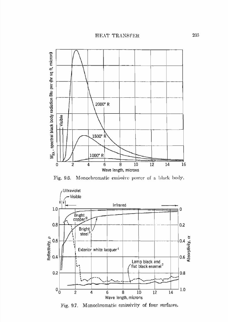
7/16/2019 Engenering Agriculture Perry
http://slidepdf.com/reader/full/engenering-agriculture-perry 244/422
HK\T THANSF'EH
1(\
\1\ - - - ~ - - f-----
\2000 ' R
Q)
\a'<ii:>
r . ~~ L 1000' R ~ t:::::-
o 2 4 6 B 10 12 14 16
Wave length, microns
Fig. 9.6. Mono('hromatic cllli>'sin' po\\"CI' of a blaek hody.
1.0
O.B
0.2
(
Ultraviolet
((ViSible
'i \. f+--------
Bright
,h c o p ~ ~)\ Bright i)
steelOI
Infrared -------_
- - - ~-
I
ExteriO: white lacquer 4,
III Lamp black and
{flat black enamel7
"I
\ ... - .... _;:;... .......... , .
' ....... .......... ...- ..- - - ~ , - - .. ................ ~ \ / . - ~
2 4 6 8 10 12 14Wave length, microns
Fig. 9.7. Monochl'ol11ati<: e m i ~ s i \ ' i t y of f01l1' A1II'f'lurs.
o
0.2
( i
0.4 )3.
~o
0.6.2<>::
O.B
1.0

7/16/2019 Engenering Agriculture Perry
http://slidepdf.com/reader/full/engenering-agriculture-perry 245/422
236 AGRICULTURAL I'IlOCESS ENGINEElUNG
can be n w a ~ l I l ' e c l directly in the laboratory (with proper precau
tion" to lllinimize and coned for eOllvection and countcrradia
t.ion) at lWl'mal temperatures and up to as high temperatures asthe material can endure. Since moan values depend upon tem
perature as ,yell as monochromatic emissivity, the temperature
should be stated when a value ()f emissivity is given, as in Table
fl.3. Emissivitics do not change n J l P ] " ( ~ c i a b l y with temperatul'e
below 600°F.
Tahle ru NORMAL TOTAL EMISSIVITY OF
VARIOUS SURFACES *
SU1jace
Aluminum, polislwd plateAluminum, oxidized at ll100F
Gopper, polishedCopper, heated to 11100FPolished ironGround sheet steel
Oxidized ironSteel plate, roughNickel, 98.9% pure, polishedNickel plate, heated to lllOoF
Zinc, 99.1% pure, polishedGalvanized sheet iron, fairly bright
Galvanized sheet iron, gray oxidizedAsbestos, paperEnamel, white fused on ironGlass, smooth
Oak, planedSnow-white enamel varnish on rough iron
plateFlat black lacquerOil paints, 16 different, all eolorsAluminum paint, 10% AI, 22% lacquer
bodyAluminum paint, 26% AI, 27% laequer
bodyAluminum paints, v!1rying age and Al
contentPaper
Porcelain, glazedRoofing paperWater
*Aclapted from McAdams. 12
Temperat1tre,OF
7:3
arJO-llIO
2·12390-1110800-1880
1720-2010
212100-700440-710390-1110440-620
8275
100-7006672
70
73100--200
212
212
212
212567269
32-212
Ernissillitll
0.0400.11-0.19
0.0280.57
0.144-0.3770.55-0.61
0.7360.94-0.970.07-0.0870.37-0.48
o 045-0 .0,5:3
0.2280.276
0.93-0.9450.8970.937
0.895
0.9060.96-0.980.92-0.9fi
0.52
0.8
0,27-0.670.924-0.944
0.9240.91
0.95-0.953

7/16/2019 Engenering Agriculture Perry
http://slidepdf.com/reader/full/engenering-agriculture-perry 246/422
HEAT TRANBFER 237
9.19. Absorptivity. In the tran;,;fcr (If radiant energy, ab
tiol'ption is ati important as emi;,;siun. Bodies that ( ~ l l l i t radiant
('llergy can abo nhwrh it. The radiant energy ab:;orbecl is converted into heat. Roughly, hollies that are good emitter:; nrc al:;o
good absorbers. At normal temperatures, a surface that a good
absorber in the visihle region of the spectrum appears black to
the eye lJecllllse it reflects no radiation, and, heing at normal tem
perature) iL also elllits Hone in the visible region. A ::;ignificant
alllount of energy in the visiJJlc region is emitted at high tempera
tures. l ~ ( ) r cxamplc, at 2000°F, a blaek line on a ('hinn plate
appears brighter than the white surface be('ausc, being a betterabs()]'ber than the white in the visihle region, it is in this region
a better emitter.
Monochromatic absurptivities 0:;-,. arc usually measured in
directly by measul'ing reflectivities P'A. For opaque objects,
impinging energy is either absorbed or reflected; therefore
0: = 1 - p.
It can be proved that
(9.47)
This can be generalized into 0: = € for gray and black bodies; but
for selective absorbers the generalization applies only when they
are absorbing at the same temperature at which they nre emit
ting. Mean absorptivity depends not only upon lllonochromatic
absorptivity but also on the spectral distribution of the i m p i n g ~mg energy,
(9.48)
in which ri\. is the monochromatic irradiation) Btu per (hI' sq ft
micron).
r is the total irradiation, Btu pel' (hr sq ft).
Example. Find the absorptivity for white paint shown in Fig. 9.7, forblack-body radiation from It surface at 540'F (1000 e R).
From li'ig. !l.B, black-body raditltion at 1000 D R is seen to be confined totllP rE'giol1 from 3 to 15 microns. Since the white paint i8 II. good reflectoronly in wave lengths less than 3 microns lIud has a relatively constant absorptivity of about 0.12 from 3 to 15 microns, its absorptivity in this rangecan be taken by inspection from the curve at 0.12. A more precise value
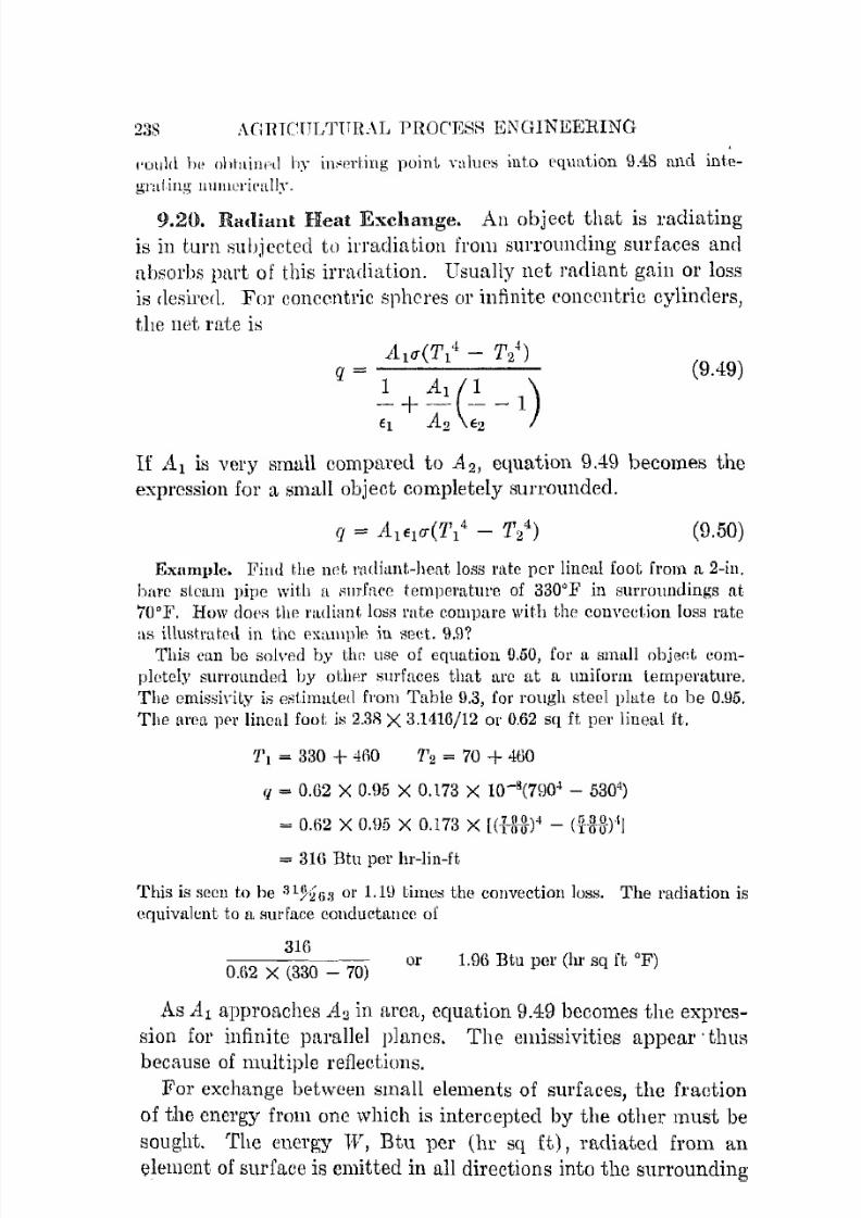
7/16/2019 Engenering Agriculture Perry
http://slidepdf.com/reader/full/engenering-agriculture-perry 247/422
2 : ~ S AGHICTJLTlTIL\L PROCESS ENGINEERING
I'uulll Ill! nhtailll·t\ by inol'rhllg point ynhlP:; into l'qulltion 9.48 Il!ld inte
graj,ing 1 l 1 1 1 1 l ( : 1 · i ( ' a l l ~ r .
9.20. Radiant Heat Exchange. An object that is radiatingis in turn subjected to irradiation from surrounding surfaces and
absorhs part of this irradiation. Usually net radiant gain or loss
is rlesircrl. For concentric spheres or infinite concentric cylinders,
the !let rate is
(9.49)
I f .A.1 is very small compared to A 2 , equation 9.49 becomes the
expression for a small object completely surrounded.
(9.50)
EXllml'le. Find the lld. l'ariianL-hc[tt loss rate per lineal foot from a 2-in.
IHll'c stl:llm pipe with a Amfnee temperature of 330'F in surruundings at
70'F. Huw clOt,:,; j,lw m<iiant 100R rat.e eompal'c with the convection loss rate
as illustmted in the examplp in sect. 9.9?This can bo soh·ed by til<> use of equatiol1 0.50, for a smull objed eOll1-
pletcly surrounded by othpl' RUl"faces that arc at a uniform temperature.
The emissh'ity is esLimuLelJ from Table 9.3, for rough steel plat.e to be 0.95.
The area ]ler linenl fooL is 2.3R X 3.1416/12 or 0.62 Sf[ it. ]leI' lineal H.
'1\ = 330 + 41\0 7'2 = 70 + 160
If = 0.(l2 X 0.95 X 0.173 X 10-8(71)0. - 5304)
= 0.(\2 X 0.\)5 X 0.173 X l(i8S)" - (Htg·)I]
= 3IG Btu per hr-lin-ft
This is seen to he 31%6:J or 1.1U times the convection loss. The radiation is
equivuJcnt to a Stu' face conductance of
31G
0,(12 X (330 - 70)or 1.9(\ Btu per (hI' sq ft OF)
As Al approaches A2 in area, equation 9.49 becomes the expres
sion for infinite parallel pInnes. The emissivities appear' thus
because of multiple reflections.For exchange between small elements of surfaces, the fraction
of the energy from one which is intercepted by the other must be
sought. The energy lV, Btu per (hI' sq i t) , radiated from an
element of surfac:e is emitted in all directions into the surrounding
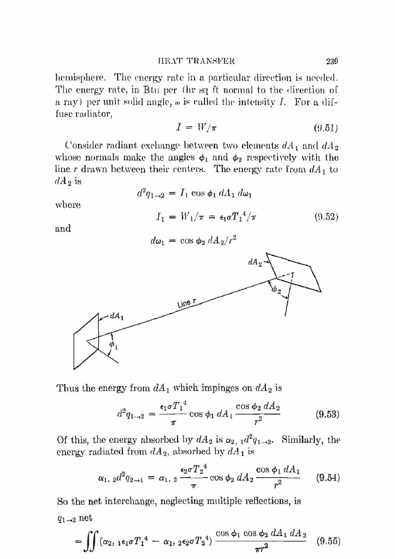
7/16/2019 Engenering Agriculture Perry
http://slidepdf.com/reader/full/engenering-agriculture-perry 248/422
fIE.\T TRANHFER 230
lH'miHphere. The (,Bergy rate in a particular direetiol1 is IlC'PriPfl.
TlIp energy rate, in Btu pel' (Ill" sq ft normal to the direction of
I i ray) per unit Holid angle, '" ii' ('alll'ri tIl(' iIltl'Ill:'ity 1. For a rliff u ~ e radiator,
1= lV/rr «(1.51)
Consider radiant exehangp between two e J p m ( ~ n t : ; ciA 1 and dAz
whose normals make the angles CPl and rPz respcetiyely with the
line 1" drawn between their ceniprs. The energy ratp from clAl to
dA 2 is
where
(\).52)
and
Thus the energy from dAl whirh impinges on dA 2 is
(9.53)
Of this, the energy absorbed by dAz is az. l(j2Q1->2' Similarly, theenergy radiated from dA z1 ttbsorbed by dA 1 is
So the net interchange, neglecting multiple reflections, is
ql ....2 net
fJ 4 01 cos CP1 cos CP2 dAl dAz=J .. (a2 , lEluT l - a i , 2 E2UT 2 ) 7rT2
(9.54)
(9.55)

7/16/2019 Engenering Agriculture Perry
http://slidepdf.com/reader/full/engenering-agriculture-perry 249/422
2'10 AGHICfTI/fURXL PROCESS E N G I N E E R I N G ~Define 11 shape bctor F 1 as the fraction of the energy emitted
from i l l which f:tlls on ..12 ; also define F2 as the fraction from.:1 2
which falls OIl . t i l ' With theRc definitions equation 9.5,5 can be rewritten as
(9.56)
From equation ~ ) . 5 6 , it can be Heen Ull1t if T2 = 1\, then
(9.56a)
Since these t l r t ~ simply geometric relationships, equation 9.56a
must be generally tl'lle. Also, if the spectral natlll'e of TV I is
about the same as W 2 , then the absorptivities and emissivities arc
equal. Substitute in equation 9.5H the equivalent of A2F2 and
also that of a l = €! and a2 = f2 , to obtain
(9.57)
From equations 9.5,5 and~ L 5 ( 3 ,
it can be seen that
(9.58)
(9.59)
When Al and A2 are small compared with 1'2,
(9.60)
(9.61)
Example. Find the net radiant-energy rate from the inside top surfaceof an oven, 18 in. by 20 in. in size, at 50QoF, and the top of a cake 9 in.
square, which is l1t 160°F and is 8 in. below the oven top. 'fhe center ofthe pan is directly below the long axis of the oven and 4 in. in front of thecenter of the top.
'fhiB problem can be solved by equation 9.57, but first the shape faetor,
or fmction of rlldillut energy from tho top which strikes the cake, must be

7/16/2019 Engenering Agriculture Perry
http://slidepdf.com/reader/full/engenering-agriculture-perry 250/422
HEAT THANNF'F.R
found. DbC the ltPlJroximalioll of equatiun \l.GO. The ir'llgth of line joining
the centers of the oUl'flleCS j" v' (·jl:!):! + ( i - 1 ~ ) ~ = 0.745 ft . The I:lurfaceo
being parallel, eos <P1 -= cos <P2 = ( ~ b ) / 0 . 7 4 5 = 0.S9S. The [ll'Pll at' the pl ln
A:J = (1)12)2 or 0.5625 'CJ fL.
P 0.S08 X 0.808 X O.5tl2.5'1 = -- 3.Hltl X 0 . 7 4 5 ~ - - = 0.25
Thl' Q m i ~ s i v i t y of the btl' ' '] top, from tht' data of TlIh]p \),3 for oxidized ~ t ( ' e l ,iR r&timatp([ at, O.S. TIH' ahsorptivity of till' ('al;:(' iH pstimlLtcd to ])(' (J.n.
T1 = 500 + 160 = \HiO. '1'2 = lliO + !tiO = 520. l"ro!U r(l'latioll \).57
q = 0.8 X 0.0 X (18 X 20)/144 X 0.20 X 0.173 X 1O-8(I)(jO! - 520!)
= 558 Btu pl'r hI'
Note that thiR is a heat rate, at. tllP cakr, of 568/0.5625 or 1010 Btu pel'
(h r sq ft.). Thr equivalent radiution ulluriU(·tau('e thus 1010/( 500 - 160)or 2.97 Btu per (hI' sq ft OF).
The accuracy of the approximation for the slwpe factor eoulrl
be impruved by dividing the a1'ea into a number of s u h n r c a ~ and
finding the shnpe factor of eae·h.
Shnpe factor::; for anumber
of simple plane figurc::; sueh asparallel plane discs, squares and l'c('tanglc::l, aclj accnt l'cctangleA
in perpendicular planeH, ami an element tlA. anti a parallel rcc
tangle have been published by HoUel 12 fmrl by Moon. l:] A 8illlple
mechanical intcgrator for irregulnl' ubjucti:i, devised by HoUel,
was used by Raber and Hutehinson 1& to measure shape factors for
Rtanding and sented persons.
'Where surface nreas nre large witll respect to the di::;tanre be
tweenthem, i.e.,
r ~ /A approl1('hrs zeru, llluitiple reflcctiulls mustbe considered. Instead of the product of the emissivities that
appears in equation 9.57, the emisHiYity raetor in equatioll 8.49
should be used.
Calculation is often simplified uy treating radiation ,vith an
equivnlent Rurfar'c ('on(lucLance, clefiner! by
(9.ti2)
(9.ti2a)
(9.G2b)

7/16/2019 Engenering Agriculture Perry
http://slidepdf.com/reader/full/engenering-agriculture-perry 251/422
242 A(::R1CULTURAL PROCESS ENGINEERING
Example. Find the equivalent slll'faec conrluetance for radiation from 11
stud pipe at 3:10' F to Slll'l'Ollnciings at 70'F, if the emissivity of the l'ough
steel slll'faee is OJ)5.
FroIll l1<[uat.ioll 0.(;2(1
Tl = 330 + 400 = 70QOR
1'2 = 70 + ·JGO = 530 oR
'1'", = (7\10 + 530)/2 = (lOocR
r [7f)0 - 530 -]2}Ii,. = 4 X 0.05 X 0.173 X lO-R X HOO:! ) 1 + 7; ~ 3 0
I. 1)0 +a ..
= 0.00li02 X 0.05 X (Ui:l(l + 0.0388)
= 1.nG Btu pm (hI' S( j ft °F)
9.21. Heat Balance, Radiation Included. A steady-state
l'ndiation phenomenon r e q u i r e ~ that the heat involved be t r a n ~ ferred from a source or to a sink as sensible heat, as latent heat,
or as eleetrical or chelllieal heat. For exalllple, a sample of grain
being dried hy an infrared lamp is receiving radiant energy at a
lllueh fasterrate than it
isemitting
it.The net
receipt is dissijlntecl [li:i latent heat for evaporating the moisture to be removed,
plus hent concluder! frum the surface through the Illass and heat
from the surface as cOllvected heat. Mathematienlly this is
where q = net radiant income, Btu pel' hr.
w = drying rate, Ih moist.ure per hr.
(9.63)
hg = hent. eontcnt of the \vater vapor at the tempemtlll'c atwhich it leaves the sYi:item.
hI = heat eontent of the moisture to he evaporated at t l .
h" = cOllveetive-heat-tmnsfm- coefficient, sUl'faee at t1 to
passing air at t:l'
Note that the dependent yariable" are ho and ht which are related
to t1 and tao The surface telllperature 11 in equation 9.63 (T',!"
equation 9.57) is (lependent upon the jrradiation f1l1c! upon the
ciissipat.ing ability of the system as defined hy equation 9.49.Note that equation 9.63 ean operate as written or by any com
hination of pal'li5. Radiation rceeiyed by a wall ii:> d i ~ s i p a t e c l by
conduction and convection. An objeet suspended by a thin wire
would dissipate net radiation by eonveetion. only.
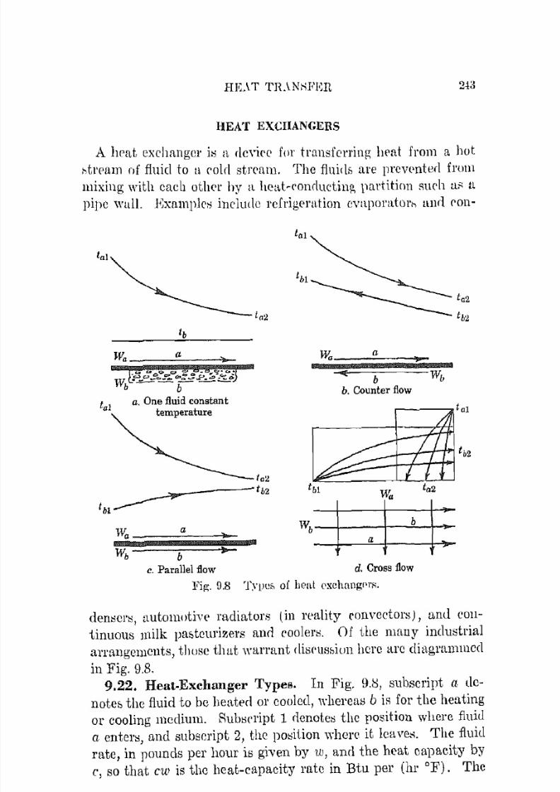
7/16/2019 Engenering Agriculture Perry
http://slidepdf.com/reader/full/engenering-agriculture-perry 252/422
HK\.T TH.\'NHFEn
HEAT EXCHANGERS
A hrat exchangc}' il:i a device for trnnsferrinp; heat from a hot
;-,tl'Pum of fluid to 1I cold strcam. The fluids are Ill'CVented from
mixing with cach other by a ltcat-ronductin[!, partition Rurh as it
pipe wall. E x a m ) l k ~ ineludc rcfrigc>mtioll cvaporatol'c, aBrl rOI1-
ta l
a
tr;'3 U o G ~ : . . ' : ; ; I c;;: cPob""r::t;_.e:.'l¥NdW l . ~ ~ ~ " ' ~ ~ )b b
a. One fluid constant
temperature
a
b
a
bb. Counter flow
c. Parallel flow d. Cross flow
1lig. 9.8 T ~ ' j J e ~ of held ('xchung(·I'R.
dem;cn;, automotivE' radiators (in reality convectors), and {'OIl
tinuous Jt1ilk lla:;tcurizers and ('Dolen;, Of the nHmy industrial
arrangemcnts, those that warrant disf'llSsiun herc arc diagramll1ed
in Fig. 9.8.9.22. Heat-Exchanger Types. In Fig. 9.1:::, subscript a de
note:;, the fluid to be heated or cooled, whereas b is for the heating
or cooling medium. Subscript 1 rlenotes thc position where fiuicl
a enter::;, and subscript 2, the position where it leave". The fluid
rate, in pounds pel' hour is given by Vi, and the heat capacity by
c, so that C'W is the heat-capacit.y rate in Btu pel' (hr OF). The
7/16/2019 Engenering Agriculture Perry
http://slidepdf.com/reader/full/engenering-agriculture-perry 253/422
2.H AGRICULTURAL PROCESS ENGINEERING
o\'el'-allunit ( , 0 1 H l l l r ~ t u n c c from fluid a. to fluid b is U Btu per (h1'
Sf(
ft, "F).The exchanger where one fluid it': constant in temperature is
~ h o w n in Fig. 9.Sa. Fluid b is ('onst:.1nt in tellllleratme because
it ii:i undergoing n change of state, gaining or losing energy as it
evaporates or condenses. This is also a special case where fluid
b, without changing state, has slH'h n high rate of flow that it
experiences practically no change in tempemtul'e.
In the counterflow exchangel', Fig. 9.Sb, fluids a and b move in
opposite dil'ed,ions. Fluid ([ ean thus be brought nearly to the
t.emperatUl'l:' at. which fluid b enters if enough surface area is
provided.In the parallel-flow exchanger, :Fig. 9.Se, with hoth fluids 1110\'
ing in the same direction, fluid (L cannot possibly be brought to
the entering temperature of fluid b. The mean temperature dif
ference is obviously smaller in the parallel-flow arrangement than
in counterflow, so that [ t greater surface urea is required. This
al'rangement. is therefore 8el(10m ·used.
In the ( ~ l ' O s s - f i o w exchanger, t.wo fluids move in it number ofseparate parallel channels arranged so that the streams of fluid a
cross those of fiui(l b, as in the automobile radiator. The several
streams of fluid (L do not mix with each ot.her until after leaving
the heat-exchange surface, as is also true for fluid b. This ar
rangement is less effective t.han cOllnterflow, hut better than
parallel flmv. I t is used because of convenience in IJroviding for
the supply and removal of the fluid streams at relatively large
rates of flow and short traverses of surface.9.23. Heat-Exchanger Analysis, One Fluid COllstant in
Tcmpel·atUl'c. Analysis of t.emperature differences in a heat
exchanger can he illustratecl by the type in Fig. 9.Sa with one
fluid constant in temperature. Idealizations required here are:
1. The fluids gain 01' lose nu heat, except t.hrough the transfer
surface.
2. The speeifi c heat and over-all thermal conductance do notchange with temperature.
3. The fluid is completely mixed at any point, so that its tem
perature at any point is uniform.
4. Heat is not conducted in the direction of fluid flow by the
walls nor by the fluids.

7/16/2019 Engenering Agriculture Perry
http://slidepdf.com/reader/full/engenering-agriculture-perry 254/422
HEAT TRANSFEH 2<i:i
5. No leakage of flui(l oeem::;, then'ful'l' t i l l ' rate of finw i:-; till'
same at any elelllent of the ::;urface.
With these idealization:;, the heal, wltieh if) traul'fcl'l'cd through
an elemeni, of Hurfa('c riA. ('aUiiCS a change in temperature of fillir! ( l ,
(9.(j-!)
The neglttive Hign indicates that fluid a drops in temperature
when t" is higher than tb. Separal iug the variables for intrgl'ationbetween definite limits
(9.65)
·With th , U, and C"W(1 eonHtant, this readily integrates to
(9.6G)
The dimensionlcHs ratio in equation H-fi6 of UA 2, the over-all
conductance or heat-transferring ability per degree temperaturedifference, to CaW", the heat-capacity rate or heat rate requiredper hour per degree Fahrenheit ehange in Huiel temperature is asignificant criterion for transfer in heat exchangers.
From equation 9.6G
(9.G7)-- = e CalVa
tal - tb
Equation 9.67 can be recognized as the expression for the "bypass" factor for an air-cooling roil discussed in Section 10.15.
Example. Find the telllperaturc to which milk will be cooleu by a direct
('xpansion surfacc cooler with a constaut refrigcl'Unt temperature of 33°F ifthe milk rate is 1 gprn (516 Ib pel' hl'), the initiltl temperature is 80°1''' the
('ooler arC'[l is 10 sq ft , and the over-all thermal COlluuctance iH 110 Btu pel'
(hI' sq ft of). The speeific heat of milk is 0.93 Btu per (lb OF).
ta2 - 33 1 1
so - 33 = ll U x 10 = e2.28 = \),75~ 0 . U 3 x 516
ta2 = 33 + (SO - 33)/9.75 = 33 + 4.S2 = 37.S2°F
The effectiveness, or change in temperature in proportion to
the maximum possible change, is a useful characteristic of a heat-

7/16/2019 Engenering Agriculture Perry
http://slidepdf.com/reader/full/engenering-agriculture-perry 255/422
246 ACnnCULTURAL PHOCE:3S ENGINEERING
exchnnge : i y ~ t e m . Denoting the l ' f f e e t i v e n e s ~ for t h i ~ case, where
Olle Jiuid eOll:"tant in telllperatme, as Eo.
(\J.GS)
Note that
(9.(\9)
and substituting from eqlHLtion 9.(\7 into ~ H i H , !l,ml then into 9.08,
(\).70)
The mean tempemture difference, At", often useful in heat
exchange calculations, is defined by
!::..l", UA 2 = C"W,,(tul - t,d (9.71)
Solving for D.t", in 9.71 and then substituting the value of UAd
t"W I I from equation D.()I)
(tul - til) - (if!2 - tb)!::..lrn ""' (9.72)
In (tn I - till "2 - iii)
'fIJi::; mean tempcrnture diffel'euec is seen to be logarithmic
mean of the initial and final differences.
9.24.. Analysis of Counter- and Parallel-Flow Exchangers.
Analytie expressions for the counterflow and parallel-flow exehangel's can be derived in a manner similar to the procedure used
in the previous section. In theBe cases t'l is not constant, but an
expression for it CUll be found from ta, the fluid heat-capacity
rates and appropriate terminal temperatures. Integration of the
differential equations yields, fol' the eounterflow effectiveness E"
(see Fig. B.9 for notation).
_ !:. e-I(I - I/TI)UA2Ic""'a]
(9.73)
R
In equation 9.73, R is the ra,tio of the hellt-capaeity rates, CbWbl
C"Wa• R is usually equal to or greater than L When R = 1,
equation \).73 becomes indeterminate. For this special case, thesolution is
(9.74)
Curves for values of Eo are given in Fig. 9.9.
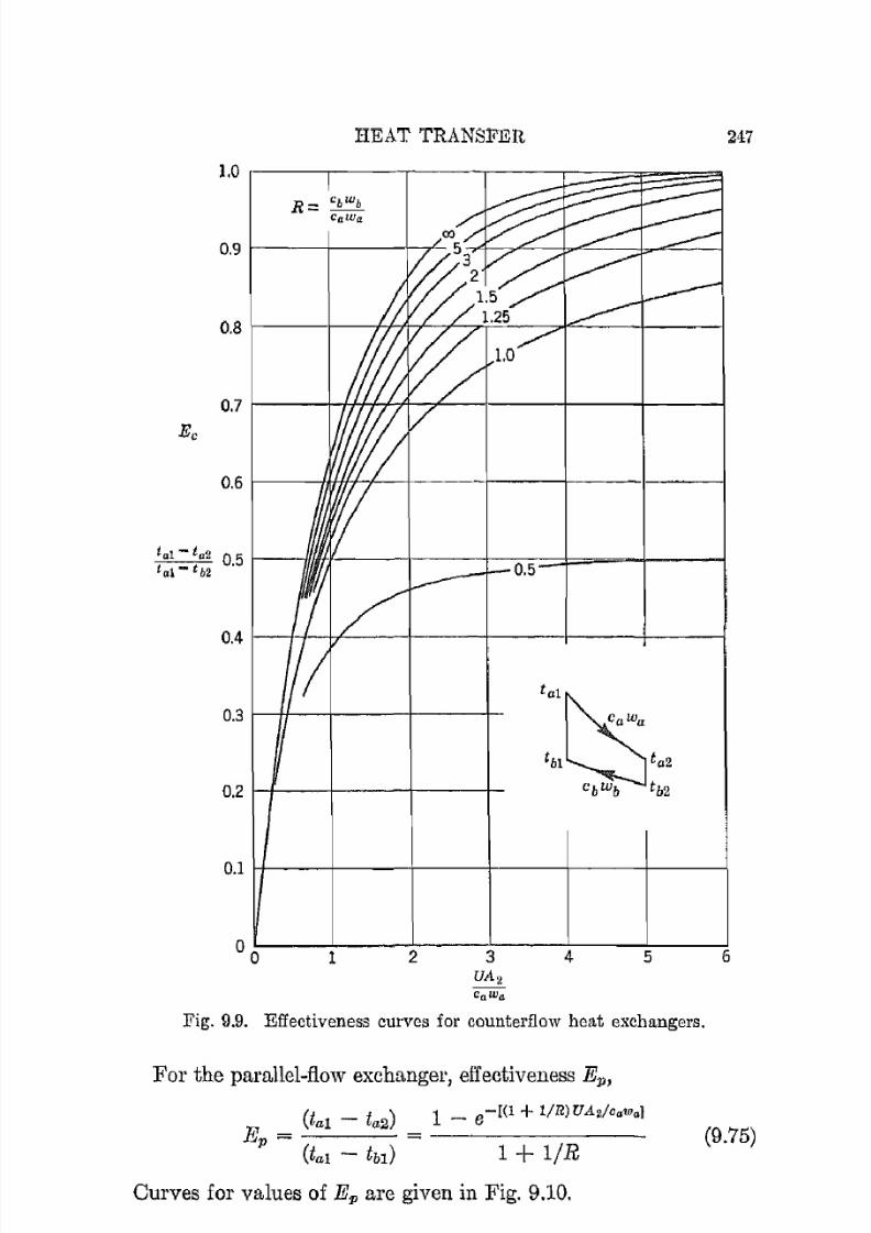
7/16/2019 Engenering Agriculture Perry
http://slidepdf.com/reader/full/engenering-agriculture-perry 256/422
IlEAT TRANSFER 247
0.2 i - I - --+----- i - --_t_
ta1t;aWu
tbl ta2cbwb tb2
0.1 f - t - - -+ - - -+ - - -+ - - - -+ - - - -+ - - - - - - 1
2 4 5 6
Fig. 9.9. Effectiveness curves for counterflow heat exchangers.
For the parallel-flow exchanger, effectiveness Ep ,
Ep = (tal - ta2) = 1 - e - [ ( l + l /R)UA
2/Ca
lO.}
(tal - tbl) 1 + l/R(9.75)
Curves for values of Ep are given in Fig. 9.10.
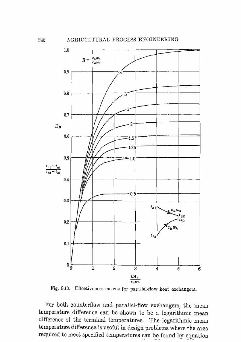
7/16/2019 Engenering Agriculture Perry
http://slidepdf.com/reader/full/engenering-agriculture-perry 257/422
248 AGmCULTUHAL PROCESS ENGINEERING
1.0I ~ ! - - - - -
R = Cb'"b
LaWa
V.9
i_ I--'
II
,/5
,L"_3-f,.--
I/;;_ _ _ 2
~ ~ ~ 1 . 51----1.25
I
'IVr- ' l ~ilLVI
0.8
0.7
Ep
0.6
0.5
0.4
f y - 0.5
J ' O , ~ " a2
2 tb2
cbwb
tb l
0.3
o.
o. 1
0_l 1
a 2 4 5 6
Fig. 9.10. Effectiveness Clll'ves for parallel-flow heat exchangers.
For both counterflow and paeallel-flow exchangers, the mean
temperature difference can be shown to be a logarithmic mean
difference of the terminal temperatures. The logarithmic mean
temperature difference is useful in design problems where the area
required to lUeet specified temperatures can be found by equation
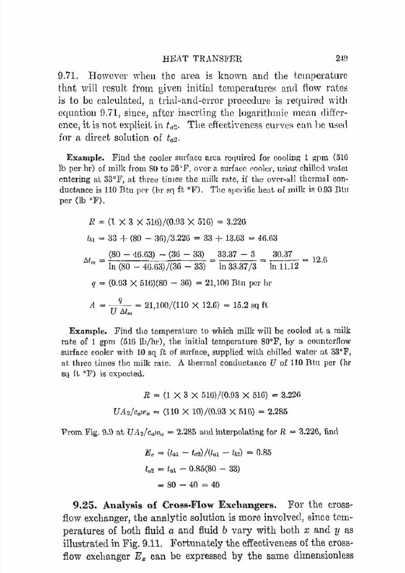
7/16/2019 Engenering Agriculture Perry
http://slidepdf.com/reader/full/engenering-agriculture-perry 258/422
HBAT TRANSFER 2Ml
9.71. However when the area is known and the temperature
that will result from g,ivell initial tcmperatul'm; and flmv rate::;
iti to be calculated, a triakmd-crl'ol' proccdlll'C is required "lvithequation 0.71, since, after inserLing the logarithmic menn diffrr
ence, it is not explicit in t l l ~ ' TlIe effectiveness curves crm be \ l ~ e dfor a direct solution of taZ'
Example. Find the cooler slll'face arca, rcl[lIil'ed for cooling 1 gpm (516
Ib per hI') of milk from 80 to 36 c Ji', over a surf:W(c ('ooler, usia),; chilled watel
entering 11L 33°F, at three times the milk rate, if the oVC'I'-:tll thermal con
ductl1nce is 110 Btu p('1' (hI' RCj ft °F). The sjJ(wific heat of milk iR 0,93 Btu
per (lb of).
R = (1 X 3 X ;)16)/(0.03 X 510) = 3.220
ib l = 33 + (80 - 3fi)/3.220 = 33 + 13.03 = 4G.fi3
At = (80 - 'l6.fi3) - (36 - 33) = 33.37 - 3 = 30.37 = 12.0
II I In (80 - 40.(3)/(36 - 33) In 33.37/3 In 11.12
q = (0.g3 X 510)(80 - 30) = 21,100 Btl! per hr
t q ( .f = -U = 21,100/ 110 X 12.6) = 1,5.2 sq f i/).1",
Example. Find the temperature to which milk will be cooled at a milk
mte of 1 gpm (5IG Ib/hl'), t.he initial temperature 80°F, by a counterflow
surface cooler with 10 sq i t of surface, supplied with chilled water at 33°F,
at three times the milk rate. A thermal conductallce U of 110 Btl! pel' (hI'
sq ft OF) is expected.
R = (1 X 3 X 5W)/(O,03 X 510) = 3.226
UA.2/C a1/)a = (110 X 10)/(0.93 X 5IG) = 2.285
From Fig. 1).1) at, Urh/cuw" = 2.285 u,nu interpolating lor R =' 3.226, fim\
Eo = (tal - t0 2) IUal - tb2) = 0.815
la2 = ta l - 0.85(80 - 33)
= 8 0 - 4 0 = 4 0
9.25. Analysis of Cross-Flow Excllangers. For the c r o s s ~flow exchanger, the analytic solution is more involved, since t c m ~peratures of Loth fluid a and fluid b vary with Loth x and y as
illustrated in Fig. 9.11. Fortunately the effectiveness of the c r o s s ~flow exchanger Ell) can be expl'essed by the same dimensionless

7/16/2019 Engenering Agriculture Perry
http://slidepdf.com/reader/full/engenering-agriculture-perry 259/422
250 AGRICULTURAL PROCESS ENGINEERING
1.0
Ex
0.2 I-/----!----I----+
0.1 ~ - - + - - - + - - - +
2 4 5 6
Fig. 9.11. Effectivelless curves for cross-flow heat exchangers.
parameters UA2/CaWa and R as the simpler heat exchangers.
Values * .15 of Em given in Fig. 9.11 indicate that the cross-flow
exchanger is between the counterflow and parallel-flow exchangers
in effectiveness.
'" Personal communication. R. Seban, University of California, 1952.

7/16/2019 Engenering Agriculture Perry
http://slidepdf.com/reader/full/engenering-agriculture-perry 260/422
HEAT TRANSFER 251
REFERENCES
1. Boelter, L. M. K., ct a1. Heat Transfer Notes. Universit.y of CaliforniaPress. 1916.
2. Brown, A. I., l\ud Mareo, S. M. Inil'odlwtion to Heat TJ'allsjm'.McGraw-Hill. 1942.
3. Carslaw, H. S., and Jaeger, J. C. CondzlClion of Heat in Solids. Ox
ford. 1947.
4. Dunkle, R. V., et al. Thc1'1nal Rudiation P1'Oject 10 Repol't, CodeNR015-202. Univ. of Calif. Inst. Eng. Res. 1950.
Ii. Dusinberre, G. M. Nllmel'ical Analysis of Heat Flow. McGraw-Hill.
1949.6. Emmons, H. W. Numerical Solutioll of Purtial Differenti[l\ Equations.
Quarterly of Applied AlatiLematics 2:173-195. 19H.
7. Gier, J. T., ct a1. Absolute Spectral Retiectivity of Cel'tain Pigments
and Metals in the Wavelength Range Between 2 und 15 ,Microns.
Thel'1rial Radiation Project 7 Report, Corle NR015-202. Univ. of
Calif. Inst. of Eng. Res. 1949.
8. Heatin{], Ventilatin{], and Air Conditioning Guide. Am. Soc. of Heating
and Ventilating Engrs. 1950.
9. International Critical '1'ables 5:253. McGraw-HilI. 1929.
10. Jakob, Max. Heat Transfer. Vol. l . "\Viley. 1949.11. Rern, D. Q. Process Heat Transfer. MeGraw-Hill. 1950.
12. McAdams, W. H. Heat 1'mnsmission. Second Edition. McGraw-HilI.
1942.
13. Moon, Pany. Scicnhfic B a ~ i s of I l l ! ~ m i n a t i n g Engineering. McGraw
Hill. 1936.
14. Newman, A. B. Drying of Porous Solids: Diffusion and Surface Emis
sion Equations. Tmns. Am. Imt. Chem. Engl's. 27 :212-2H. 1931.
15. Nusselt, W. A New Heat Transfer lTornmla for Cross Flow. Tech
nisc/"e M echanik Thermodynamik 1, No. 12. 1930.w. Raber, B. F., and Hutchinson, F. W. Optimum Surface Distribution in
Panel Heating and Cooling Systems. IIeating, Piping, Ail' Condi
tioning 15 :602-614. 1943.
17. Southwell, R. V. Relaxation Methods in Engineering Science. Oxford.
1940,
PROBLEMS
1. Fiud the rate of heat loss pel' sq ft from the hot-air supply duct of a
spray (hying chamber. The duct is insulated with a 2-in. layer of glassfiber batts. The inner surface temperature is 300°F, the outer, 75°F.
Thermal conductivity k of the batts = 0.025 Btu per (hr sq ft of per
ft).
2. A heat exchanger built with 16-gage copper tubes has un over-all unitconductance of 300 Btu per (hr sq ft OF) under certain operating COll-
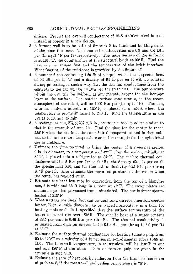
7/16/2019 Engenering Agriculture Perry
http://slidepdf.com/reader/full/engenering-agriculture-perry 261/422
252 AGRICULTURAL PROCESS ENGINEERING
ditions. Predict the over-all conductance if lS-S stainless steel is used
instead of copper in a new design.
3. A furnace wall is to be built of firebrick 8 in. thick and building brickof the same thickness. The thermal conductivities are 0.9 and 0.4 Bt.uper (hr sq ft of per i t) respectively. The iuner surface of the firebrickis at 1800°F, the outer surface of the structural brick at 90°F. Find theheat rlLte per sCluare foot and the temperature oI the brick interface.Wlmt haction of the resistance is provided by the firebrick /
11. A number 2 can containing 1.25 Ib of a liquid which has a specific heat
of 0.9 Btu per III OF unci a density of 64 ]b per cu it will be rotated
during processing in such a way that the thermal conductance from thecontents to the can will be 10 Btu pel' (hl' sq ft OF). The temperature
within the r.:an will be uniform at any instant, except for the laminarlayer at the surface. The outside smface conductance, in the steam
atmosphere of the retort, will be 1000 Btu per (hr sq ft OF). The can,with its contents initially at 160°F, is placed in a retort where the
temperature is promptly raised to 240°F. Find the temperature in thecan at 5, 10, and 15 min.
5. A rectangular c ~ m , 2Vs X 3% X 6 in., contains a food product similar to
that in the example of sect. 9.7. Find the time for the center to reach235°F when the can is at the same initial tcmperaturG and is then subject to the saIlle retort temperature as in the example for the cylindrical
can in problem 4.6. Estimate the time required to bring the center of a spherical melon,
9 in. in diameter, to a temperature of 42°F after the melon, initially at
SO°F, is placed into a refrigerator at 35°Ji'. The surface thermal conductance will be 5 Btu pe\' (hI' sq ft OF), the density 62.'1 lb per eu ft ,
the specific heat 0.90, and the thermal conductivity 0.25 Btu per (hr sqft OF pcr ft) . Also estimate the moan temperature of the melon whenthe center has reached 42'F.
7. Estimate the heat loss rate by convection from the top of a blancherbox, 6 ft wide and 36 ft long, in a room at 7()OF. The cover plates are
aluminum-painted galvanized iron, uninsulated. The box is direct steamlleated at 210°F.
8. What wattage per lineal foot can be used for a direct-immersion electricheater, :}'f; in. outside diameter, to be placed horizontally in a tank forheating molasses? I t is specified that the surface temperature of theheater must not, rise over 180°F, The specific heat at a water contentof 22.5 per cent is 0.46 Btu per Ob OF). The thermal conductivity isestimated from data on sucrose to be 0.19 Btu per (hr sq it OF per ft)at 68°F.
9. Estimate the surface thermal conductance for heating tomato pulp from
60 to 170'F at 11 velocity of 4 I t per sec in l-in.-diametel' tubes (0.88 in.ID). The tube-wall temperature, in counterflow, will be 120°F at oneend and 180°F at the other. Data on tOIllato pulp are given in the
example in sect. 9.13 .
.10. Estimate the rate of heat loss by radiation from the blancher box covel'of problem 8, if the mean wall and ceiling temperature is 75°F.
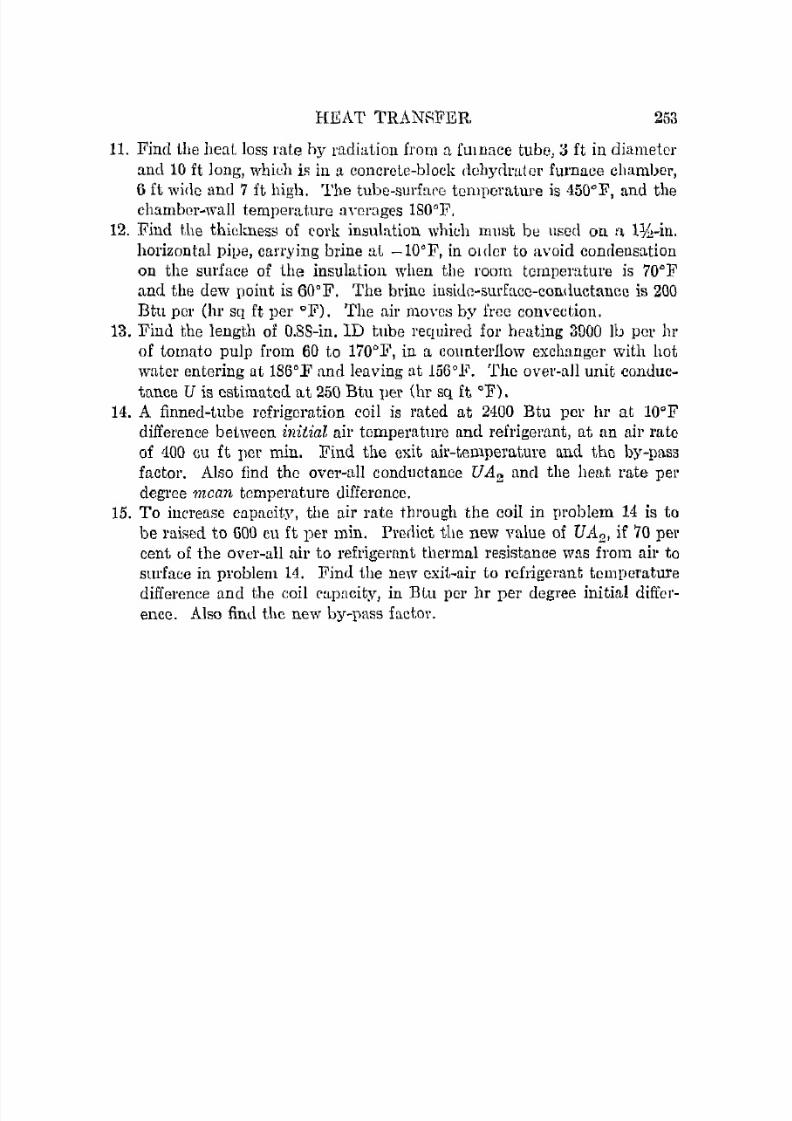
7/16/2019 Engenering Agriculture Perry
http://slidepdf.com/reader/full/engenering-agriculture-perry 262/422
HEAT TRANRFER. 253
11. Find the heal loss rate hy rildiation from a [milace tube, ::l ft in diameter
and 10 ft long, whidl is in a concrete-block (lchyrlrater furnaee chamber,
6 ft wide and 7 ft high. The tube-surface temperature is 450°F, and thec h a m b c r ~ w a l l temJlentture ann'ages lS0°F.12. Find the thiekness of cork insulation whieh m l l ~ t be used on n, lYoJ-in.
horizontal pipe, carrying brine at -10°F, in Older to avoid conrlensMionon the surface of t.he insulation when the room tcmperature is 70°Fand the dew point is 60"F. The brine insilie-snrf[ICc-con<iuctanee is 200
Btu per (hI' sq ft per OF). The ail' 1ll0\'CS by free convection.
13. Find the length of O.SS-in. ID tube required for heating 3!l00 lb pel' hI'
of tomato pulp from 60 to 170 oP, in a counterflow exchanger with hotwuter entering at 186°F and leaving at 156"F. The over-all unit c o n d \ 1 c ~taD.ce U is estimated at 250 Btu ller (hr sq it OF).
14. A finned-tube refrigeration coil is rated at 2,100 Btu per hI' at lOoFdifference between initial ail' temperature and refrigerant, at an uir rate
of '100 eu ft rIel' min. Find the exit air-tempemture and the by-passfactor. Also find the over-all conductance UA2 and the heat rate pel'degree mean temperature difference.
15. To increase capacity, the nil' rate through the coil in problem 14 is to
be raised to GOO eu ft per min. l'mdict the new value of UA 2 , if 70 pel'cent of the over-ull air to refrigerant thermal resistance was from air tosurface in problem 14. Find the new exit-air to rcfrigerant temperature
difference und the coil c[Lpncity, in Btu per hr per degree initial difference. Also find the new by-pass factor.

7/16/2019 Engenering Agriculture Perry
http://slidepdf.com/reader/full/engenering-agriculture-perry 263/422
CHAPTER 10
Air-Vapor Mixtures
(The Psychrometl'ic Gha.rt)
NOMENCLATURE
11 ""' area, sq ft.B = by-paRs factor, dimensionless.fv = surface vapor conductance, lb per (hI' sq ft lb pOl' sq ft).f = surface heat. transfer, Btu pel' (hl' sq ft OF).
I I = absolute humidity, Ib moisture pel' Ib dry air.ha = heat content of an atmospheric mixture, Btu pel' Ib dry air.
hj g = latent heat of evaporation, Btu per lb.hg = heat content of water vapor, Btu per lb.M = molecular weight.
N = number of pouud moles, weight in pounds divided by molecular weight.p = pressure, Ib per sq in. absolute.
Pa '" pressure exert,ed by dry ail', lb pel' sq in.pat = atmospheric pressure, Ib pel' sq in. = p" +p" = pressure exerted by the water vapor ill the atmosphere when saturated,
1b per sq in.Po = pressure exerted by the water vapor ill the atmosphere when unsatu-
ru,ted, Ib per sq in.q = heu,t rate, Btu pel' hr.R = universal gas constant := 1545, It Ib per (lb mole OR).T = absolute temperature, OR = OF + 460.
(, = temperature, OF.
ta = air temperature, OF.
t,o = wet-bulb temperature, OF.
V = gas volume, eu ft.V = hmnid volume, eu ft per Ib dry air.
Va. = volume of l1b dry air at saturated conditions, cu ft.
= volume of lIb water vapor at saturated conditions, eu ft .W = quantity of gas, lb.w = evaporation rate, 1b water per hr.
In the field of processing, air is used as a heat-transfer medium,
a source or sink for water vapor, a source of oxygen for combus-
254
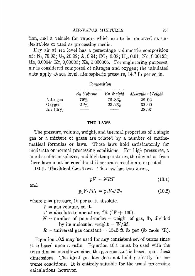
7/16/2019 Engenering Agriculture Perry
http://slidepdf.com/reader/full/engenering-agriculture-perry 264/422
AIR-VAPOR l\IIXTUREH 25;'
tion, and n vehicle for vapors whir.h are to be 1'emovecl a6 undet:;irables or used as processing media.
Dry air at sea Ie-'i'el has a percentage volumetric composition
of: N2 , 78.03; O2,20.99; A, 0.94; CO 2 , 0.03; I h 0.01; Ne, 0.00123;He, 0.0004; K1', 0,00005; Xe, 0.000006. For eng,inecl'ing purposes,air is considered composed of nitrogen and oxygen; the tabulated
data apply aL sea level, atmospheric pressure, 14.7 lb per sq in.
NitrogenOxygenAir (dry)
Composition
By Yol7l1ne
79%21%
By Weight
76.8%23.2%
THE LAWS
Molecular Weight
28.0232.0028.97
The pressurc, volume, weight, and thermal properties of a single
gas or a mixture of gases are related by a number of mathe
matical formulas or laws. These laws hold satisfactOl'ily formoderate or normal proceRsing conditions. For high pl'essures, a
numbcr of atmospheres, and high temperatures, thc deviation fro111
these laws must be considered if accurate results :1re expected.
10.1. The Ideal Gas Law. This law has two forms,
pV = NRT (10.1)
and
(10.2)where p = pressure, lb per sq i t absolute.
V = gas volume, eu ft.T = absolute temperature, OR (OF + -100).
N = number of pound-moles = weight of gas, Ib, divided
by its molecular weight = W / M.R = universal gas constant = 1545 ft Ib per (lb mole OR).
Equation 10.2may
be used forany
consistent sct of terms sinceit is based upon a ratio. Equation 10.1 must be used with the
term dimensions shown since the gas constant is based upon these
dimensions. The ideal gas law docs not hold perfectly for ex
treme conditions. I t is entirely suitable for the usual processing
calculations, however.
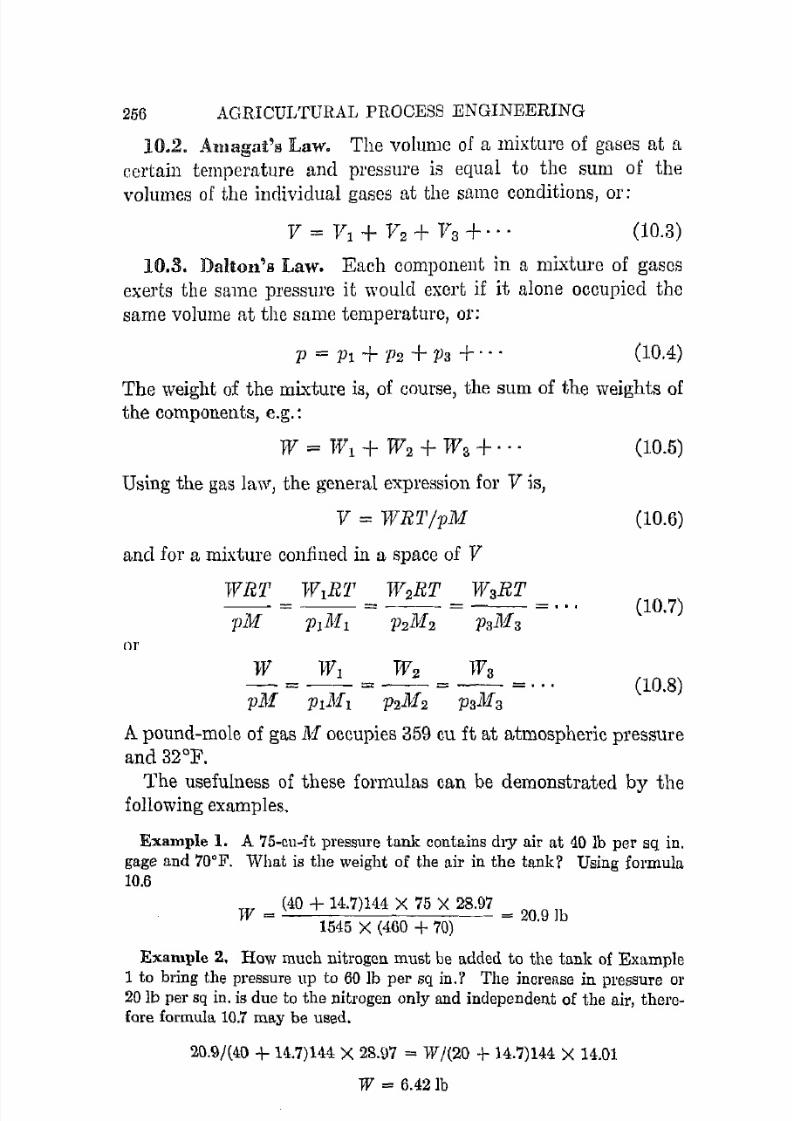
7/16/2019 Engenering Agriculture Perry
http://slidepdf.com/reader/full/engenering-agriculture-perry 265/422
256 AGRICULTURAL PROCESS ENGINEERING
10.2. A m a g a t ~ 8 Law. The volume of a mixture of gases at a
certain temperature and pressure is equal to the sum of the
volumes of the individual gases at the same conditions, or:
(10.3)
HUt. Dalton's Law. Each component in a mixture of gasesexerts the same pressure it ,vould exert if it alone occupied the
same volume at the same temperature, or:
P = PI + P2 +Pa + .. (10.4)
The weight of the llli..xture is) of course) the sum of the weights ofthe components, e.g.:
(10.5)
Using the gas law, the general expression for Vis,
V = WRT/pM (10.6)
and for a mixture confined in a space of V
WRT WIR7' W2RT WaRT-- = - -_ = - -_ = - -_ =.' . (10.7)pM PI M1 P2M2 Pa 1113
01'
W WI W2 TVa-=--=--=--= . . (10.8)pM P1 l111 P2M2 Pa ll1a
A pound-mole of gas M occupies 359 cu ft at atmospheric pressureand 32°F.
The usefulness of these formulas can be demonstrated by thefollowing examples.
Example 1. A 75-cu-ft pressure tank contains dry air at 10 lb per sq in.gage and 70°F. What is the weight of the air in the tank? Using formula10.6
TV _ (40 + 14.7)144 X 75 X 28.97 _- 1545 X (460 + 70) - 20.9 lb
Example 2. How much nitrogen must be added to the tank of Example
1 to bring the pressure up to 60 lb per sq in.? The increase in pressure or20 Ib per sq in. is due to the nitrogen only and independent of the air, therefore formula 10.7 may be used.
20.9/(40 + 14.7)144 X 28.97 = W/(20 + 14.7)144 X 14.01
W = 6.421b
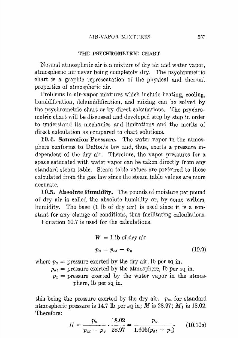
7/16/2019 Engenering Agriculture Perry
http://slidepdf.com/reader/full/engenering-agriculture-perry 266/422
AIR-VAPOR l\UXTtTREfi 2:i7
THE PSYCHROMETRIC CHART
Normal atmospheric ail' is a mixture of (11'y air and water vapor,
atmospheric nil' never being completcly dry. The psychrometric
chart is a gruphic l'epl'esentution of the physical and thermal
properties of atmospheric air.
Probloms in air-vapor mixtures which include henting, cooling,
humidification, (lehumidification, and mixing can be solverl by
the psychrometric chart or by direct calculations. The psychro
metric chart will be discussed and developed step by "tep in orderto undel'st,and its mechanics and limitations and the merits of
direct calculation as compared to chart solutions.
10.4. Saturation Pressure. The water vapor in the atmos
phere conforms to Dalton's law and, thus, exerts a pressure in
dependent of the dry air. Therefore, the vapor pressures for a
space saturatecl with watcr vapor can he taken directly from any
standard steam table. Steam tablc values are prefel'red to those
culculated from the gas law since thc steam table vahlcs are moreaccurate.
10.5. Absolute Humidity. The pounds of moisture per pound
of dry air is called the absolute humidity or, hy some writers,
humidity. The base ( l ib of dry air) is nsed since it is a con
stant for any change of conditions, thus facilitating calculations.
Equation 10.7 is used for the calculations.
TV = 1 Ib of dry air
pa = PIt! - Pv (10.9)
where Pa = pressure exerted by the dry air, 11> per sq in.Pat = pressure exerted by the atmosphere, Ib per sq in.
1)1) = pressure exerted by the water vapor in the atmosphere, Ib per sq in.
this being the pressure exerted by the dry air. Pat for standardatmospheric pressure is 14.7 Ib per sq in; Mis 28.97; ]\1[1 is 18.02.
Therefore:
Pv 18.02 PvH= . - -=-- - - -
Pat - pv 28.97 1.605(Pat - Pv)(lO.lOa)

7/16/2019 Engenering Agriculture Perry
http://slidepdf.com/reader/full/engenering-agriculture-perry 267/422
258 AGRICULTURAL PROCESS ENGINEERING
and]Jat(UlO5)H
Pv = 1.605H + 1 (10.10b)
The linear plot with humidity and temperature as the ordinate and abscissa shown in Fig. 10.1 is the base plot for thepsychrometric chart. H may be expressed in pounds or grains
(lIb::::: 7000 grains) per pound of dry air. The more convenient
OF
Fig. 10.1. A base plot with relative "humidity and water vapor pressure.
unit will probably be used. The water-vapor pressure is calculated by equation 10.10b and is usua.lly added to the plot in the
position shown. Other positions are frequent, however.
10.6. Relative Humidity. Relative humidity is defined as
the ratio of the actual pressure of the water vapor in the air to
the pressure if the air were saturated with moisture at the same
temperature. For example, if the pressure were 0.180 Ib per sq ft
at 70°, the relative hUmidity would be (0.180/0.361) 100, or 50
per cent. This definition leads to a family of curves, partiallyshown in Fig. 10.1.
10.7. Percentage Humidity. Percentage humidity is defined
as the ratio of the absolute humidity at a state to the absolute

7/16/2019 Engenering Agriculture Perry
http://slidepdf.com/reader/full/engenering-agriculture-perry 268/422
AIR-VAPOR MIXTURES 259
humidity at the same temperature for a Baturated condition.
Relative humidity is defined as (p!Ps) 100, percentage humidity
as (HjH.) 100.AlLhough percentage humidity is more convenient for some
calculations than relative humidity, relative humidity is prefer
able when dealing with systems where equilibrium moisture content of commodities is concerned.
]0.8. Hmnhl Volume. The humid volume of an air-water
vapor mb..iure is assumed (without significant errol') to be the
sum of the volume of 1 lb of dry air and the volume of the water
vapor. The volume of 1 lb of the dry air for ally temperatureand pressure can be calculated from the gas law (10.1). Like
wise, the volume of the water vapor peT pound of dry ail' for any
temperature and humidity can be calculated from the vapor pres
sure and humidity values previously discussed. Although vapor
pressure volumes calculated thus are generally acceptable, steam
table "alues used as shown below will yield more accurate results.
T ( HVVS]1v)V = - Va.+ - - -
T. Pat(10.11)
where V = humid volume of mixture, Cll ft per lb dry air at temperature T.
T = absolute tempel'uture of the air-water-vapor mixture,RO.
T. = absolute temperature of the air-water-vapor mixture at
the saturated, dew-point temperature of the watervapor.Vas = volume of 1 Ib dry air at Ts and atmospheric pressure
Pa; calculated from the gas law.Pat = atmospheric pressure, Ib per sq in.vv., = volume of 1 Ib of water vapor, saturated, at the dew
point, cu ft per Ib (from steam table).IJv = water-vapor pressure of the atmosphere, III pel' sq in.
The isovolume lines of Fig. 10.2 were calculated by equation10.11.
The specific volume is determined thus:
Specific volume = Humid volume/ (1 + H) (10.12)

7/16/2019 Engenering Agriculture Perry
http://slidepdf.com/reader/full/engenering-agriculture-perry 269/422
260 AGRICULTURAL PROCESS ENGINEERING
H
OF
Fig. 10.2. Humid volume and total heat dattt arc added to the base plot
thus.
10.9. Total Heat! Enthalpy. The total heat or enthalpy ofan air-water-vapor mixture is expressed by
ha = O.24t+ Hhg (10.13)
where ha = heat content of the mixture, Btu per 11 of dry air, re
ferred to zero degrees for air, and to water at 32°F
for vapor.
O.24t = average specific heat of dry air (0.24) times the tem
perature.
or
and
H = humidity.
hg = heat content of a pound of water vapor at temperatUl'e
t. This can be taken directly from t1 steam table
or can be cnJculated from
hg == 107,5.2 + 0.45 (t-32)
hg = 10GO.8 + 0.4St
ha = O.24t + [{(1060.8 +0.45t)
(10.14)
(1O.14a)
(10.15)
which is sufficiently accurate for most engineering applications
below a partial vapor pressure of 2 Ib per sq in. The constant
1075.2 is the heat content of a pound of water vapor at 32 D F j
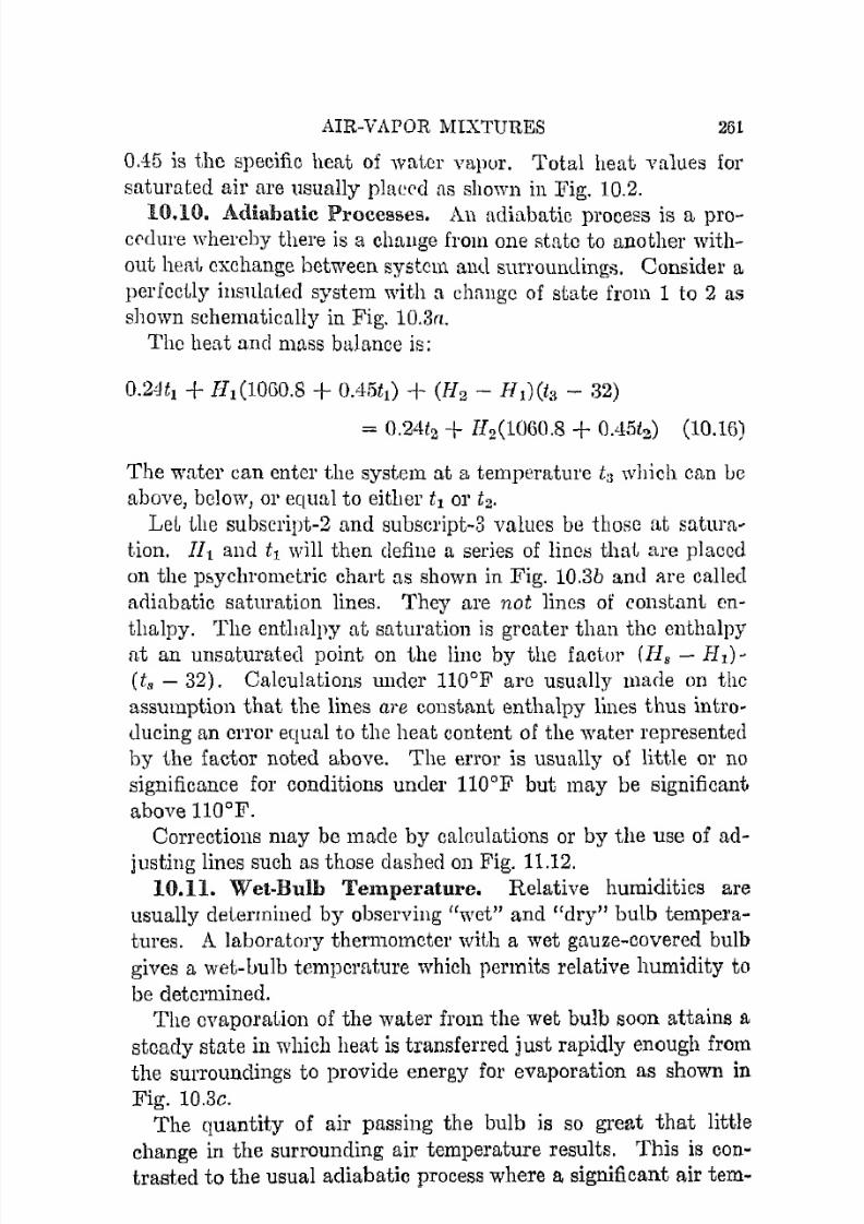
7/16/2019 Engenering Agriculture Perry
http://slidepdf.com/reader/full/engenering-agriculture-perry 270/422
AIR-VAPOR MIXTURES 261
0.45 is the specific heat of water vapor. Total heat values forsaturated air are usually plae('d as shown in Fig. 10.2.
10.10. Adiahatic Proccsses. An adiabatic process is a procrdure whereby there is a change from one state to another with
out heat exchange between system lilKl sU1'l'oundings. Consider a
perfectly insulated system with a change of state from 1 to 2 asshown schematically in Fig. 10.3(1.
The heat ancl mass balance is:
0.24tl + HI (lOGO.8 + 0.45tl) + (H2 - Ht)(ta - 32)
= O.24tz + H2(1060.8 + OA5tz) (10.16)
The water can enter the system at a temperature ta which can ucabove, below, or equal to either t l or t2.
Let the subscl'ipt-2 and subscl'ipt-3 values be those at s a t u r a ~tion. I I and t l will then define a series of lineH that are placedon the p5ychrometrie chart as shown in Fig. 10.3b and are calledacliabatic saturation lines. They are not lines of constant en
thalpy. The enthalpy at saturation is greater than the enthalpyfit an unsaturated point on the line by the factor (II. - H I )
(t. - 32). Calculations under 110°F arc usually made on thc
assumption that the lines are constant entha1py lines thus intro
ducing an error equal to the heat content of the water representedby the factor noted above. The error is usually of little or no
significance for conditions uncleI' 110°F but may be significant
above HO°F.Corrections may be made by calculations or by the use of ad
justing lines such as those dashed on Fig. 11.12.
10.n. Wet-Bulh Temperature. Relative humidities are
usually determined by observing "wet" and "dry" bulb temperatures. A laboratory thermometer with a wet gauze-covered bulb
gives a wet-bulb temperature which permits relative humidity to
be determined.The evaporation of the water from the wet bulb soon attains a
steady state in which heat is transferred just rapidly enough from
the surroundings to provide energy for evaporation as shown in
Fig. 10.3e.The quantity of air passing the bulb is so great that little
change in the surrounding air temperature results. This is c o n ~trasted to the usual adiabatic process where a significant air e m ~

7/16/2019 Engenering Agriculture Perry
http://slidepdf.com/reader/full/engenering-agriculture-perry 271/422
Air vap.or mixture11 }{z
(a)
ts Hs Ps
g " fA",-'"r I" t,Alp, - p,)
taHaPa.Fig. 10.3. An adiabatio process, shown schematically, is keyed to the totalheat scale by adiabatic saturation lines (a). The lines represent the processwhen sub-2 and sub-3 values are at saturation. The wet-bulb process (b)
is also represented by the adiabatic saturation lines.
262
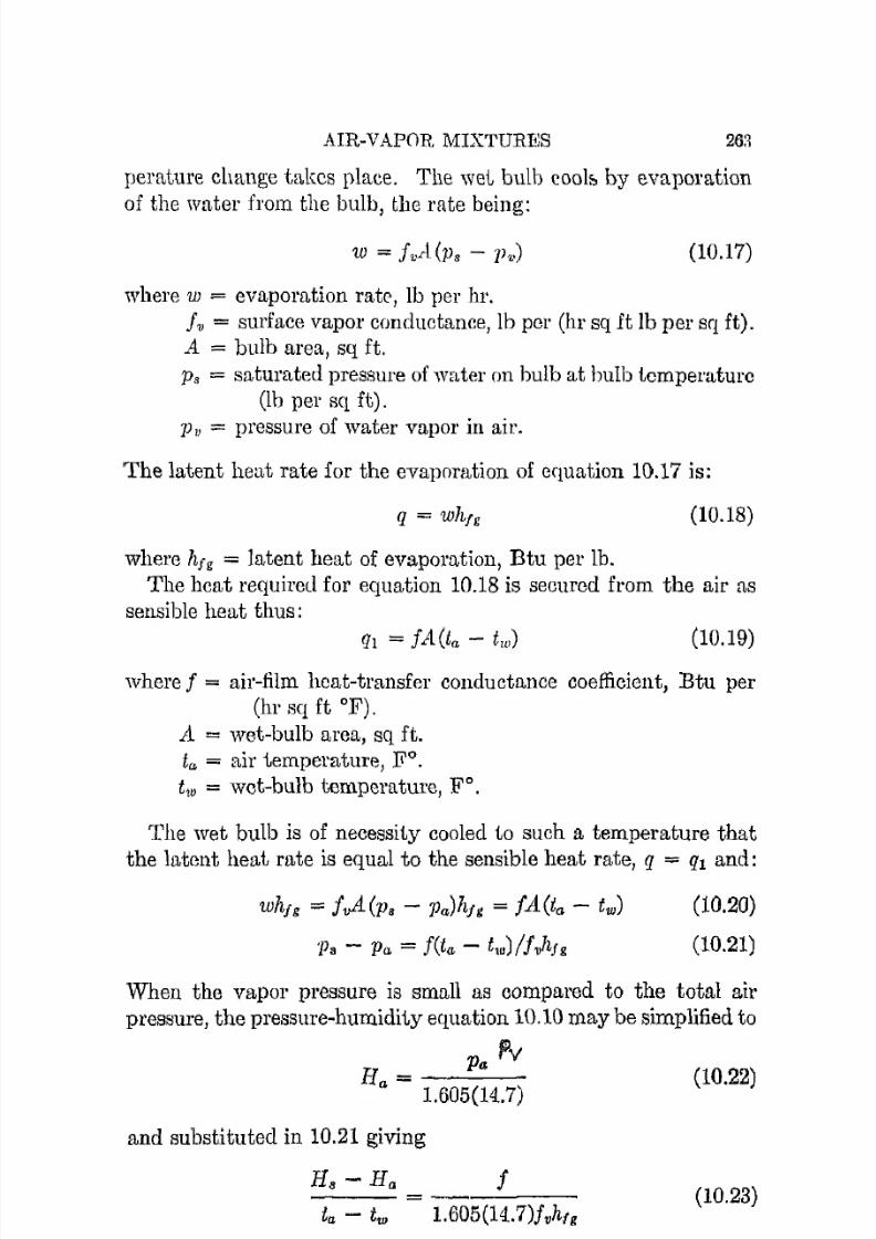
7/16/2019 Engenering Agriculture Perry
http://slidepdf.com/reader/full/engenering-agriculture-perry 272/422
AIR-VAPOR MIXTURES 2 6 ~
perature clu\nge takes place. The wet bulb eool::, by evaporationof the water from the bulb, the rate being:
(10.17)
where w = evaporation rate', lb per hr.Iv = surface vapor conductance, Ib per (hI' sq it Ib per sq ft).A = bulb area, sq ft.
Ps = saturated pressure of water on bulb at bulb temperature(lb per sq ft).
JJv = pressure of water vapor in air.
The latent heat rate for the evaporation of equation 10.17 is:
q = Whig (10.18)
where htg = latent hea.t of evaporation, Btu per lb.The heat required for equation 10.18 is secured from the air as
sensible heat thus:
(10.19)
where f = air-film heat-transfer conductance coefficient, Btu per(hI' sq ft OF).
A = wet-bulb area, sq ft.ta = air temperature, FO.
t10 = wet-bulb temperature, FO.
The wet bulb is of necessity cooled to such a temperature that
the latent heat rate is equal to the sensible heat rate, q = ql and:
Whig = ivA-(p. - Pa)hfg = fA(ta - tw)
'Pa - pa = f(ta - t,u)lf1lhfg
(10.20)
(10.21)
When the vapor pressure is small as compared to the total airpressure, the pressure-humidity equation 10.10 may be simplified to
Pv
Iia = 1 . 6 0 ~ ~ 4 . 7 ) (10.22)
and substituted in 10.21 giving
H8 - Ha f---- (10.23)
ta - tw 1.605(14.7)fvh(g
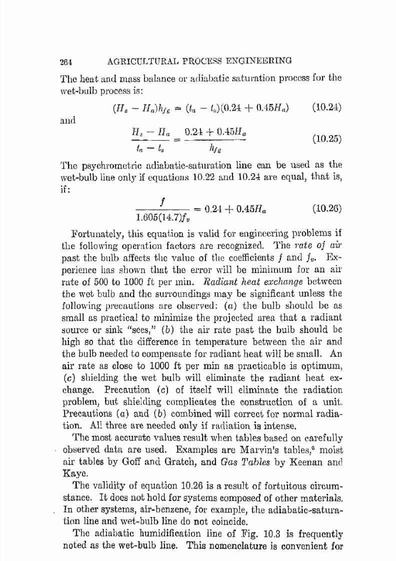
7/16/2019 Engenering Agriculture Perry
http://slidepdf.com/reader/full/engenering-agriculture-perry 273/422
264 AGRICULTURAL PROCESS ENGINEERING
The heat and mass balance or adiabatic saturation process for the
wet-bulb process is:
(10.24)
and
l-Is - II" 0.2+ + OA5H"(10.25)
f" - ts hfg
The psychrometrie adiabatic-saturation line can be used as thewetrbulb line only if equations 10.22 and 10.2+ are equal, that is,
if:
- - ' - - = 0.2cl + 0.45H"1.605 (1 ".l:.7)fv
(10.26)
:B'ol'tunately, this equation is valid for engineering problems if
the following operation factors are recognized. The rate oj airpast the bulb affects the value of the coefficients j and jv. Ex
perience has shown that the error will be minimum for an ail'mte of 500 to 1000 ft per min. Radiant heat e:cc}wnge between
the wet bulb and the surroundings may be significant unless thefollowing precautions are oDserved: (a) the bulb should bc assmall as praetical to minimize the projected area that a radiant
source or sink i tsees ," (b) the ail' mte past the bulb should behigh so that the difference in temperatl1l'e betwecn the ail' and
the bulb needed to compensate for radiant heat will be small. Anair rate as olose to 1000 ft per min as practicable is optimum,
(0) shielding the wet bulb will eliminate the radiant heat ex
change. Precaution (0) of itself will eliminate the radiationproblem, but shielding complicates the construction of a unit.Precautions (a) and (b) combined will correct for normal radiation. All three are needed only if radiation is intense.
The most accurate values result when tables based on carefullyobserved data are used. Examples are Marvin's tables,G moist
air tables by Goff and Gratch, and Gas Tables by Keenan andKaye.
The validity of equation 10.26 is a result of fortuitous circumstanoe. I t does not hold for systems composed of other materials.In other systems, air-benzene, for example, the adiabatic-saturation line and wet-bulb line do not coincide.
The adiabatic humidification line of Fig. 10.3 is frequently
noted as the wet-bulb line. This nomenclature is convenient for

7/16/2019 Engenering Agriculture Perry
http://slidepdf.com/reader/full/engenering-agriculture-perry 274/422
AIR-VAPOR MIXTURES 265
the ca/:lual user, but it is erroneous as l'l'glll'(h, the true pro]Jtrtiesof the line.
USES OF THE PSYCHROMETRIC CHART
10.12. State Factors. The information thHt CI111 be s<'curedfrom the psychrometrir chart for a sLate condition is shown in
t t Wet taDew bulbPOint
Relativehumidity
Humidvolume
Hs P,
Fig. 10.4. Information that can be secured from a psychrometric chartfrom one state point.
Fig. lOA. Note that the crossing of any two property lines estab
lishes :1 state point from which all other values can be secured.For example, 70°F air having a wet-bulb temperature of 55°F
has a humidity H of 0.006 lb of water per lb of dry air. The dew
point is 43°F; vapor pressure, 0.132 Ib pel' sq in.; relative humid
ity, 37 per cent; humid volume, 13.47 cu ft dry air; and the vaporpressure, 0.3Ci1 Ib per sq in. Note that the relative humidity can
be calculated from the ratio piPs'10.13. Cooling, Heating. Cooling or heating without chang
ing the moisture content takes place horizontally as shown in Fig.
10.5. The heat involved per pound of dry air is h2 - h1. In cool
ing, the temperature of the cooling medium must be above thedew point or dehumidification will result (see section following).

7/16/2019 Engenering Agriculture Perry
http://slidepdf.com/reader/full/engenering-agriculture-perry 275/422
266 AGRICUJJTURAL PHOCESS ENGINEERING
t1 t2
Ji'ig. 10.5. The psychrometric heating and cooling process.
10.14" Mixtm·cs. The state point of an air-vapor mixtureresulting from mixing airs of different state points falls very
~ - - - - l H 2- : : : : : . _ - - -+ - - - - - lH
3
Fig. 10.6. The psychrometric process of mixing.
nearly on a straight line connecting the two initial states, Fig.10.6. Proof of this procedure follows.
Using W as the pounds of dry air,
(10.27)

7/16/2019 Engenering Agriculture Perry
http://slidepdf.com/reader/full/engenering-agriculture-perry 276/422
AIR-VAPOR MIXTURES 267
and ~ ~ + ~ ~ = ~ ~ ( W ~:. Ha = (W]H l + lV2H 2)/(H'1 + H'2) (10.29)
The heat required to cool TV2 from tz to f3 must equal the heatrequired to heat WI from tl to t3, so that
Wt(ts - i I )(0.24 + 0.45Hl ) = W 2 (t2 - ta)(0.24 + OA5H2 ) (10.30)
t3 - t l W2(O.24 + 0,45H2). -. - - -
From equation 10.20
WI (0.24 + OA5H 1)
(H3 - H l )/(H2 - Ha) = W2 /W t
(10.31)
(10.32)
Elimination of WdTVl from equutions 10.31 and 10.32 and solution for t3 yields
113 - HI 0.24 + 0,45li2t! + t2 .-----
H2 - H3 0.2·1 + 0,45HI
fa = ------------]fa - H! 0.24 + 0.45H2
1+ . ~ - - - -H2 - H3 0.24. + OA5H!
(10.33)
However, when 0.24 + 0,45H2 : : : 0.24 + OA5H!, equation 10.33
can be simplified to
tlH2 - t2Il! + H3(t2 - tl )f3 = (1O.33a)
H2 - HI
In equation 10.33a, i3 is seen to be linear with H 3 , as represented
by the straight line of Fig. 10.6. The approximation is adequate
for Il}any engineering problems.Example. Find the temperature that will result when air at 50°F with
a humidity of 0.007 is mixed with enough air at 110°F and a humidity of0.028 to give a humidity of 0.021 in the mixture. Equation lO.33a yields
i3 = L50 X 0.028 - 110 X 0.007 +0.021(110 - 50)]/(0.028 - 0.007) == 90°F
The precise solution from equation 10.33 is ta ::: 90.505°F.
10.15. Cooling, Dehumidifying. Where a stream of air at a
temperature t2 (Fig. 10.7) comes in contact with a heat-removingsink at a temperature, to, below the dew point, the state point of
the cooled air falls on a straight line as shown in Fig. 10.7. The
location of the final state point is depcndent upon the heat-trans
fer characteristics of the medium separating the cooling material
and the air.
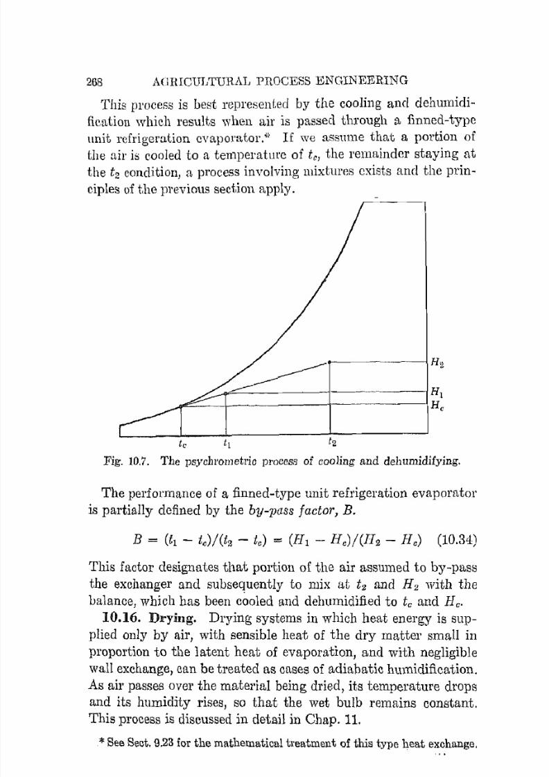
7/16/2019 Engenering Agriculture Perry
http://slidepdf.com/reader/full/engenering-agriculture-perry 277/422
268 AClHICULTUHAL PROCESS E N G I N J i ~ E R I N GThis process is best represented by the cooling and dehumidi
fication \vhich results when ail' is passed through a finned-type
unit refrigeration evaporator:' I f we assume that 11 portion ofthe air is cooled to a temperature of te, the remainder staying at
the t2 condition, a process involving mixtures exists and the prin
ciples of the previous section apply.
----I I
. , .A ' e : : : : . . . _ - \ - - - - - - - - j - - - - . - - - - \ He
Fig. 1D.7. The psychl'ometric process of cooling and dehumidifying.
The performance of a finned-type unit refrigeration evaporator
is partially defined by the by-p(lsS factor, B.
This factor designates that portion of the air assumed to by-pass
the exchanger and subsequently to mix at tz and H2 with the
balance, which has been cooled and dehumidified to to and lIe.
10.16. Drying. Drying systems in which heat energy is sup
plied only by air, with sensible heat of the dry matter small in
proportion to the latent heat of evaporation, and with negligible
wall exchange, can be treated as cases of adiabatic humidification.As air passes over the material being dried, its temperature drops
and its humidity rises, so that the wet bulb remains constant.
This process is discussed in detail in Chap. 11.
*See Sect. 9.23 for the mathematical treatment of this type heat exchange.

7/16/2019 Engenering Agriculture Perry
http://slidepdf.com/reader/full/engenering-agriculture-perry 278/422

7/16/2019 Engenering Agriculture Perry
http://slidepdf.com/reader/full/engenering-agriculture-perry 279/422
G E N E R A L ~ E L E C T R I CPIYCHROMETlllC CHART
Barometric P t ~ i 1 l ! C I M ~ 6 Lo per Sq la
Fig. 10.9, A sychrornetric chlrt, (Courtelij G e n e r ~ Electric Co,)
Copyrigh\ 1942, by Geneml E ~ c t r i c CQmpany

7/16/2019 Engenering Agriculture Perry
http://slidepdf.com/reader/full/engenering-agriculture-perry 280/422

7/16/2019 Engenering Agriculture Perry
http://slidepdf.com/reader/full/engenering-agriculture-perry 281/422
AIR-VAPOR MIXTURES 269
10.17. Ail' Couditioning. Ail' conditioning involves processesof heating, cooling, humidifying, or dehumidifying, either singly
or in suitable combination. Heating and cooling were treated insect. 10.13.
Air may be humidified by passing it through a water spray orover saturated pads thus adding moisture to the air by anadiabatic process, a-b, Fig. 10.8. The cooled ail' is then heated
to the desired temperature, b-c, Fig. 10.8.
t l
Fig. 10.8. The psychrometric ail' conditioning process.
Steam may be injected into the ail' thus increasing the humidity
from a to a without essentinl change in temperature. This procedure is rigorous except for the sensible heat to be removed tocool the steam as vapor, from its introduction temperature to theail' temperature. Precisely, the enthalpy of the mixture is thesum of the enthoJpies of the components.
Dehumidification can be brought about by passing the air
through a finned refrigeration cooler or a water spray at t2 or
brine spray at temperature ti , cooling and dehumidifying from a
to d, Fig. 10.8, then heating to e. Adsor-bants such as silica-geland activated alumina may be used to remove moisture by process
a-f, then cooling.10.18. A Psychrometric Chart. A psychrometric chart de
signed for the range 20° to 120°F is included as Fig. 10.9. This
7/16/2019 Engenering Agriculture Perry
http://slidepdf.com/reader/full/engenering-agriculture-perry 282/422
270 AGRICULTURAL P!WCEtlS ENGINEERING
chart cnn be used for allY of the state or prucess determinations
cliHcussed in previous sections. Hig. 11.12 is a similar chart for a
higher temperature range.
REFERENCES
1. Arnold, J. H. The Theory of the Psychrometer. Physics 4 :255-262,
334-340. 1933.2. Awbery, J. H., and Griffiths, Ezer. The Busic Law of the Wet and
Dry-Bulb Hygrometer at Temperatures from 40C to 100C. Proc.
Phys. Soc. (London) 4,1: 132-142. 1932.
3. Carrier, W. H., and Mackey, C. O. A Review of Existing PsychrometricData in Relation to Practical Engineering Problpms (PRO-59-7).T1"ans. A.S.M.E. 59 :33-47 (Sect. 1). 1937.
4. Dropkin, David. The Deviat.ion of the Actual Wet-Bulb Temperaturefrom the TemperaLure of Adiabatic Suturation. Cornell Univ. Ena.Expt. Sta. Bull. 23. 1936.
5. Keenan, J. H., und Kaye, J. Gas Tables. Wiley. 1948.6. Marvin, C. F. Psychrometric Tables for Obtaining the Vapor Pressure,
Relative Humidity, and Temperature of the Dew Point from Read
ings of the Wet- and Dry-Bulb Thermometers. U. S. Dept. of Comm.W.B. 235. 1941.
7. Peny, John H. Chemical Engineers Handbook. Third Edition.
McGraw-Hill. 1950.8. Raber, B. F., and Hutchinson, F. W. Refrigeration and Air Condition
ing Engineering. Pp. 148-202. Wiley. 1945.
9. Sherwood, T. !C., and Comings, E. W. Trans. Am. Insi. Chem. Engrs.
28:88-117. 1932.10. Wile, D. D. Psychrometry in the Frost Zone. Refri(]. Eng. 48:291-303.
1944.
11. Zimmerman, O. T., and Lavine, Irvin. Psychrometric Tables and Charts.Industrial Research Service. 1945.
PROBLEMS
1. Dry- und wet-bulb temperatures are 80° and 65°F respectively. Whatare the humid volume, relative humidity, water-vapor pressure, clewpoint, absolute humidity?
2. Solve problem 1 relative to the top of a 10,000-ft mountain. The
/ atmospheric pressure is 0.6876 that at sea level.(3. Atmospheric air has a temperature of 85°F and a dew point of 53°]!'.
What is the relative humidity when cooled to 60°F? How lIluny poundsoj water are removeu. from 20,000 cu It if cooled to 35°]!'?
<l.A grain drier requires 12;000 eu 11, per min of 115°F air. The atmospheric air is at 75°F and 68 per cent relative humidity. How manyBritish thermal units per hour arc required to heat the air?

7/16/2019 Engenering Agriculture Perry
http://slidepdf.com/reader/full/engenering-agriculture-perry 283/422
AIR-VAPOR MIXTURES 271
5. Ail' at 95°F and 25 pel' cent relative humidity is blown through lJ, 35°F
water spray and is cooled to 75°F. What is the relative humidity?
6. What is the error in pel' cent resulting from chart design when the heaL
required to heat 65°F air with 90 per cent relative humidity to 105°F isdetermined from the adiabatic saturation lines?
7. The relative humidity on a 90°F day is 30 per cent.
a. How many pounds of water vapor arc in a room 20 ft by 30 ft, by10 i t high?
b. What is the weight of the air-water-vapor mixture in the room above'?
c. Air is discharged from an evaporative cooler at 76°F. ·What is it s
relative humidity'?d. Will eggs removed from a 45°F storage room "sweat"? Why'?
e. I f the air is humidified isothermally, what is H at saturation?
8. A stream of air at HO°F and 10 pel' cent relative humidity merges with
a stream at 70° and gO per cent relative humidity. The temperature of
the mixture is 76°F.
a. What is the relative humidity of the mixture?
b. I f the higher temperature air stream has a rate of 9000 eu ft pel' min,
what is the rate of the lower temperature stream?
9. Ail' at 80°F and ,10 per cent relative humidity is cooled by a refrigeration
coil which has a fin temperature of 33°F. The air is discharged fromthe coil at 48°F. The ail' rate is 6000 et! ft, per min. How mauy pounds
of water are removed from the air per 24 hr?

7/16/2019 Engenering Agriculture Perry
http://slidepdf.com/reader/full/engenering-agriculture-perry 284/422
C HAP TER 11
Drying
NOMENCLATURE
A = urea, sq ft.t: = a constant, d i I l l ( ) ! l s i o n l ( ' ~ s .
cp = specific heat, Btu per (lb OF).
J)p = particle diameter, ft.Du = volumetric diffusivity, 8(1 ft ppr hr.
Dv," = wpight diffusivity of waL!:l' vapor ill air = D",/p.
E = weight. of mobture cvaporutccl, lb.
e = natuml logarithm base.F' = wet weight, lb.J = surface thermal conductance, Btu per (hI' sq ft OF).
jv = surface water-vapor conducl allCP, Ib per (hr :-;q ft lb per sq ill.).
a = woight velocity, lb per hr sq ft.
He = exhaust air humidity.
Hi = initial air humidity.h = enthalpy of humid air, Btu per lb.
hfg = latent heat of evaporation, Btu per lb.k = thermal (:oncluctivit,y, Btu Ilel' (hI' sq ft OF per it).
M = moisture content, dry basis, per cent.m = moisture content, wet basis, per cent.
lifE = eqUilibrium moisturc content, dry basis, per cent.1I1f = final moisture content, dry basis, per cent.ll;1i = initial moistllre content, dry basis, per cent.II:!s = moisture content at surface, dry basis, per cent.
n = a constant, dimensionless.P = dried weight, lb.p = toLal pressure, Ib per sq in.
Pa = pressure of water vapor in the air, lb per sq in.
P. = water vapor pressure at saturation, t., Ib per sq in.Q = quantity of water, lb.q = heat rate, Btu per hr.
rh "'" equilibrium relative humidity, a decimal.S = surface conductance, water vapor, ft pCI' hr.T = absolute temperature, OR.
272
7/16/2019 Engenering Agriculture Perry
http://slidepdf.com/reader/full/engenering-agriculture-perry 285/422
DRYING
ta = air temperature, °Ir.
t, = water-surface tempemturc, of.
V = ail' mte, cu ft per (min sq ft).TT" = vuiocity, ft per hI'.
v = humid volume, cu It per Ib tlry ail'.
Wd = weight of dry material, lb.
Wm = weight of moisture, lb.
10 = water l'olllovall'[lte, lb per mill.
:c = distance from r-enter of mass, ft.
a:" = fictive film thickness offering resistllllcC to herd; flow, ft.Xv = fictive film thickness olleTing resistallce to diffusion, ft .
(\ ! = generalize(\ drying indox, inverse hr.
a ' = specifie drying index./' = specific weight, Ib per eu ft .
IL = viscosity, lb per hI' ft .
0= time, hr.
273
The removal of moisture from a product is known as drying ot'
dehydration. Although these terms arc used interchangeablydrying is the removal of moisture to a moisture content in equi
librium with normal atmospheric ail' or to such a moisturc contcntthat decrease in quality fro111 molds, enzymic action, and insects
will be negligible-12 to 14 per cent wet basis-for most matcrials.
Dehydration is the removal of moisture to a very low moisture
content, nearly bone-dry condition. Bone-dry material is ma
terial from which all the moisture has Leen removed; the moisture
content is zero.The importance of drying farm products is increasing. Drying
permits the fanner to secure a greater economic rcturn for the
following reasons:
1. Early harvest (at high moisture content) mmmllzes field
damage and shatter loss and facilitates tillage operations for such
products as eorn, small grains, and grass seed.
2. Long-period storage without product deterioration is possible.
3. Viability of seeds is maintained ovel' long periods.
4. Production operations are facilitated for such products as
cotton and corn.
5. Products with greater economic value are produced, forexample tobadco, dried fruit, and vegetables.
6. Waste products can be converted to useful products, for
cxample livestock feed from fruit pulp and almond hulls.
7/16/2019 Engenering Agriculture Perry
http://slidepdf.com/reader/full/engenering-agriculture-perry 286/422
274 AGRICULTURAL PROCESS ENGINEERING
MOISTURE CONTENT
The moisture content of a substance is usually expressed in
jJel'ceniag,e by weight on the wet basis, i.e., in grams of moisture
per 100 g of sample.
(11.1)
where rn is moisture content, wet basis, pel' cent; IV"" weight of
moisture; TVa, weight of bone-dry materiul.
This method of expression tends to give an incorrect impressionwhen applied to drying, since both the moisture content and the
basis on which it is computed change as drying proceeds. If,
however, the moisture is expressed as moisture content, dry basis,
part::; of water per parL of "bone-dry" matter (water-free matter),
a correct representation of moisture to be removed and of drying
rate can be obtained, since the amount of dry matter remains con
stant as the moisture evaporates.
Moisture content, dry basis, per cent, 1\1[, is
M = 100(Wm/W a) = 100rn/(lOO - rn) (11.2)
The moisture contont, dry basis, is sometimes expressed as mois
ture ratio, that is, pounds of moisture por pound of dry matter or
M /100. The quantity of moisture present at any time is directly
proportional to the dry-basis moisture content.
Exumple. Find the amount of moisture to be removed in drying a tonof grain, initially at 25 per cent moisture (wet basis), to 14 pel' cent moisture
(wet basis). Also find the weight of dried grain.
Solution (a), from wet-basis moisture contents. The initial quantity of
moisttll'e is (2%00) X 2000 or 500 lb. The dry matter is 2000 to 500 or
1500 lb. The final weight of 14 per cent moisture grain is the weight ofdry matter, multiplied by the pounds of moist material per pound of dry
matter, or 1500 X 100/(100 - 14) = 1744 lb. Thus the amount of moistureto be removed is 2000 - 1744 or 256 lb.
Solution (b), from dry-basis moisture contents. The initial moisture con
tent, dry basis, is 100 X 50%500 or 33.33 pel' cent. This can also be foundtt$ 25/(100 - 25). The final moisture content, dry basis, 4«)00/(100 -14)
or 16.28 per cent. The amount of moisture to be removed, per Ion of wet
grain, is then 1500 (33.33 - 16.28)/100 or 256 lb. The yield is 2000 - 256 or
1744 lb. The amount of dry matter is 2000 X 100/(100 + 33.33) = 1500 lb.
Nate: The amount of moisture to be removed is not the initial weight

7/16/2019 Engenering Agriculture Perry
http://slidepdf.com/reader/full/engenering-agriculture-perry 287/422
DRYING 275
multiplied by the difference in wet-basis moisture contents. I t is equul to
the weight of dry matter, multiplied by the difference in dry-basis moisture
contents.
When only initial and terminal values are needed, the moisturecontent, wet basis, can, with appropriate equations, be as readilyused as the moisture content, dry basis, as shown by the following,
W;nl
500lbMoisture
Wd
1500 Ib
Dry matter
256 Ib
r-- - - - -1 /Mo is tu reI p removedI I
I I
""___ W ; , , ~~ - - - - - l - 244 IbMoisture
W,l
1500lbDry matter
F = wet weight = Wm + Wa, lb.E = weight of moisture evaporated, lb.
P = dried weight, lb.Wd = weight of dry matter, lb.
Wet Basis from IIll tu 1112 Dry Basis from lIh to M2
Pounds of moisture to be removed pel' pound of fresh material
E7lL1 - 1712
- =F' 100 - m2(11.3) !!.. = 11ft - .M2 (11.4)F Ml + 100
Pounds of moisture to be remove.d per pound of dried produce
- =P 100 - m1
11.5) !!. = Ml - M2 (11.6)P M2 + 100

7/16/2019 Engenering Agriculture Perry
http://slidepdf.com/reader/full/engenering-agriculture-perry 288/422
276 AGRICUJ,TUR,\L PROCESS ENGINEERING
IFet Basi;.; from ml to m2 Dry Basis from nil to m2
I'onnc]A of wet D1!Lk'lial to ]ll'()(lu('p a pound of dript! product
(11.7)F ]liJ + 100- = --- (11.8)P ][2+100
POUllIls of lhil'd IWOI\\ll't per pound of wpt, nUitel'hil
P 100 - TIll
P = 100 -1 /12{lUl} !!_ = i1I2 -I- 100 (11.10)
F J1I1 + 100
Pounds of mnbture 1,0 be I'PIllOVCr! {lPl' pound of dry mattf'r
E = _ 100(1111 - 1112) (11.11)
Wd (100 - rl!l)(IOO - rIl2)
E- = MI - M2 (11.12)IVrl
MOISTURE DETERII-UNATIONS
Moisture-determining procedures are classed as primary or di
rect and secondary or indirect. The primary procedures are such
that the moisture in a sample is removed and the quantity is
determined by weighing or measuring. The secondary procedures
depend upon some characteristic of the material which is related
to moisture content and must be calibrated against an official
primary method.
"Official" methods arc those that have been accepted by theAssociation of Official Agricultural Chemists and are recognized
by thc U. S. Production and Marketing Administration. Mois
tures determined by "Official" methods by certified inspectors areaccepted by the courts.
A list of methods and some commercial moisture-determinationdevices follow:
H.I. Pl'imary Methods, Oven ("Official"). Samples areground and dried in an air or vacuum oven at a temperature
close to boiling water for a prescribed time. The loss in sampleweight is considered to be moisture. Temperature and dryingtime vary from material to material. The specific procedure fureach material must be followed.
Operating conditions for a fcw materials are listed as follows.Temperatures are Fahrenheit.
Grain and stock feeds: 204 0 to 212°, 5 hI', vacuum oven; or271 0 to 279 0 ,2 hI', air oven.

7/16/2019 Engenering Agriculture Perry
http://slidepdf.com/reader/full/engenering-agriculture-perry 289/422
DRYING 277
Dried fruits: 158 0, 6 hI', vacuum oven. (Also tentative for
dried vegetables.)
Hops: 140°,3 hl', vacuum oven; 01' :218°,1 hI', air oven.Nuts (tentative): 158 0 vacuum oven, weight at 2-h1' intervals
until loss pel' interval does not vary more tlmn 3 mg pel' 2-gsample.
Dried milk powder: 202 0, 2 hI', vacuum oven.
Molasses: 140°,2 hI', vacuum oven.
Toluene distillation ("Official"): the ground sample is distilledin toluene, 232 0
, until all the water has been removed hom the
sample, about 1 hr. Xylene ("unofficial") which boils at 280 0 is
also used in this system. Both ure a fire hazard.Brown-Duvel Moisture Tester (accepted as "Official") : whole
grains are distilled in a mineral oil that has a higher boiling pointthan the (bstillil1g temperatul'C. The moistm'c that is driven off
is condensed and measured.
11.2. Secondary Methods. Electrical Resistance Meters.
Devices that measure the electl'icall'esistance of products are cali
brated against oven determinations and are adequate for manytests. Since resistance varies with the distl'ilmtion of moisture
within the material, with material density, and perhaps with acid
index and other factors and since the characteristics of the mois
ture machine itself change with time, exact results cannot beexpccted. Hay samples that contain a few wet pieces may give
a completely erroncous indication of moisture content. Material
removed from a drier for a moisture check has a moisture gradient
through each element and may also yield unsatisfactory results.S0111e studies with wheat . inclicaLe errors of a quarter of a per
cent can be expected. Errors greater than this are frequently ex
perienced. Tests can be made in a minute 01' less.Dielectric Meters. The capacitance of an electrical condenser
varies with the moisture content of a material placed between its
plates. This feature is used in dielectric meters for moisture de
termination. Meters of this type are as fast as the resistance
meters but are less accurate.5
EQUIUBRIUM MOISTURE CONTENT
Farm products, both natural and processed, contain adsorbed
moisture. The adsorbed moisture exerts a moisture vapor pres-

7/16/2019 Engenering Agriculture Perry
http://slidepdf.com/reader/full/engenering-agriculture-perry 290/422
278 AGRICULTURAL PROCESS ENGINEERING
SUl'C which vn1'ic'8 with the ll10iElture content of the material and
from material to material. The ratio of the moisture vapor pres
sure to the satUl'[1ted vapor pressure of pure water at the temperature of the material is called the equilibrium relative humidity.
A ploL of the eCluilibl'iulll relative humidity (abscissa) and mois
ture content (ol'flinate) is known as an equilibrium moisture curve.
20 30 40 50 60 70 80 90 100Equilibrium relative humidity, %
]i'ig. 11.1. Equilibrium moisture curves o.f a number of materials at roomtemperatme, approximately 77°F.
Such a plot for a number of materials is given in Fig. ILL
Materials that exhibit this charactel'istic are caned hygroscopicmaterials.
The moisture content may be given on either a wet or dry basis,
depending upon the intended use of the curves. The curves are
affected somewhat by a change in temperature, an increase in
temperature shifting the curve downward. The effect is not sufficiently pronounced to be considered in roost engineering work.
Equilibrium moisture curves can be defined by the followingequation 4
(11.13)

7/16/2019 Engenering Agriculture Perry
http://slidepdf.com/reader/full/engenering-agriculture-perry 291/422
DRYING 279
where 1'h = equilibrium relative humidity, tL decimal.
ME=
equilibrium moisture content, dry basis, per cent.T = temperature, oR.G, n = constants.
Equilibrium moisture data can, therefore, be reported in terms of
the constants c and n. Values of these constnnts for some ma
terials are given in Table 11.1.
Tahle 11.1 VALUES OF EQUILIBRIUM CONSTANTS c AND n
FOR SOl\m MATEIUALSMaterial c n
Shelled COl'll 1.10 X 10-[' 1.90Wheat 5.59 X 10⁻⁷ 3.03Sorghum 3.40 X 10⁻⁶ 2.31Soybeans 3.20 X 1O-[) 1.52Flaxseed 0.89 X 10⁻⁶ 2.02Raisins 7.13 X 10⁻⁵ 1.02Dried peaches 4.11 X 10⁻⁴ 0.564
Dried prunes1.25 X 10-'\
0.805Cotton 4.91 X 10⁻⁵ 1.70Wood 5.34 X 10⁻⁵ 1.41Spray-dried eggs 2.9.5 X 10-5 2.00Natuml day 7.5a X lO-· 1.72
The equilibrium moisture properties of materials are important.
in storage and drying. I f the relative humidity of the air in
contact with a material is higher than the equilibrium relative
humidity of the material at its current moisture content, thematerial will increase in moisture content, the moisture content
at the air relative humidity being the value approached. An air
relative humidity lower than the equilibrium will cause the mois
ture content to decrease.
DRYING PROCESSES
Drying processes can be divided into two periods: (1) the con
stant d r y i n g - l ~ a t e period, and (2) the falling drying-rate period.
11.3. Constant·Rate Period. In this period a material or
mass of material containing so much water that liquid surfaces
exist will dry in a manner comparable to an open-faced body of
water. The water and its surroundings, not the solid, will d e t e r ~
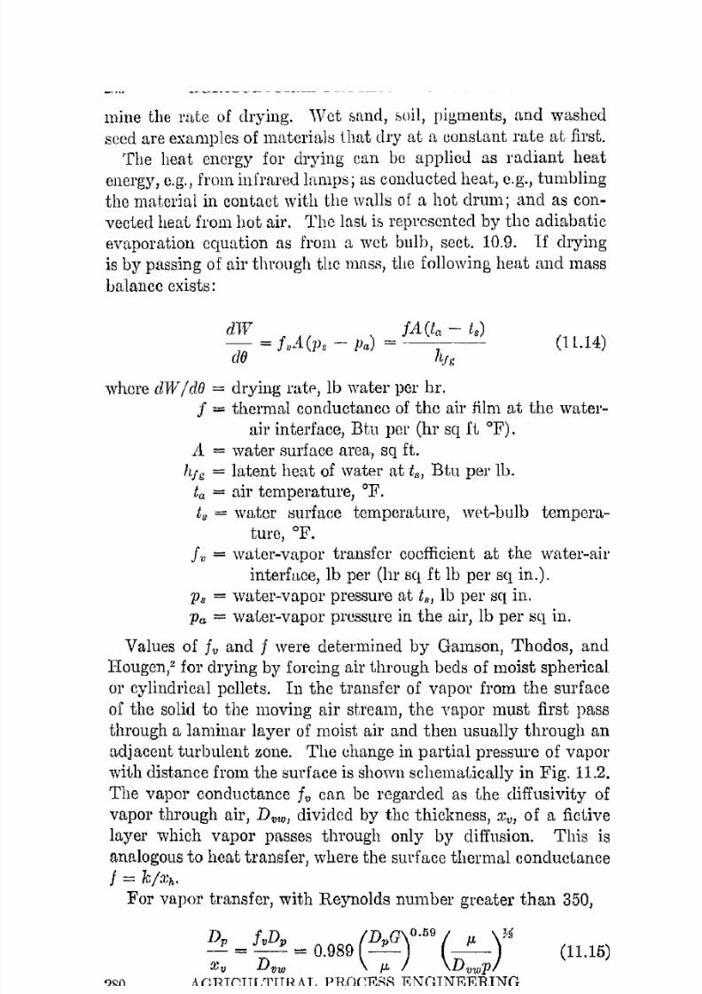
7/16/2019 Engenering Agriculture Perry
http://slidepdf.com/reader/full/engenering-agriculture-perry 292/422
2RO AGBICULTURAL PROCESS ENGINEERING
mine the rate of drying. "\Vet bund, 50il, pilSrnents, and washed
seed are examples of materiali:i that dry at a constant rate at first.
The heat energy for drying can be applied as radiant heatenergy, e.g., from infrared lnmps; as conducted heat, e.g., tumbling
the material in contact with the walls of a hot drum; and as con
vected heat from hot air. The last is represented by the adiabatic
evaporation equation as from a wet, bulb, sect. 10.9. I f drying
is by passing of nil' through the mass, the following heat and mass
balance exists:
dTV fA (ta - ts)
- = f"A (lJs - }Ja)dO hJg (1 L.14)
where dTVIda = drying ratp, Ib water per hr.
f = thermal conductance of the air film at the water
air interface, Btu por (hI' sq H OF).
A = water surface area, sq ft.
hjg = latent heat of water at ts , Btu per lb.
la = air temperature, OF.
t. = water i:iurfaee temperature, wpt-bulb temperature, OF.
f" = water-vapor transfer coefficient at the water-air
interface, lb per (hr sq i t lb per sq in.).
P. = water-vapor pressure at t., lb per sq in.
Pu = water-vapor pressure in the air, lb per sq in.
Values of tv and t were determined by Gamson, Thodos, and
Hougen,2 for drying by forcing air through beds of moist spherical
or cylindrical pellets. In the transfer of vapor from the surfaceof the solid to the moving air stream, the vapor must first pass
through a laminar layer of moist air and then usually through an
adjacent turbulent zone. The change in partial pressure of vapor
with distance from the surface is shown schematically in Fig. 11.2.
The vapor conductance tv can be regarded as the cliffusivity of
vapor through air, Dmv, divided by the thickness, Xv, of a fictive
layer which vapor passes through only by diffusion. This is
analogous to heat transfer, where the surface thermal conductancej = kjXh.
For vapor transfer, with Reynolds number greater than 350,
D f D (D G)0.59 ( )H__!!_ = ~ = 0.989 _p_ __f.1._~ D_ f.1. D_p
(11.15)
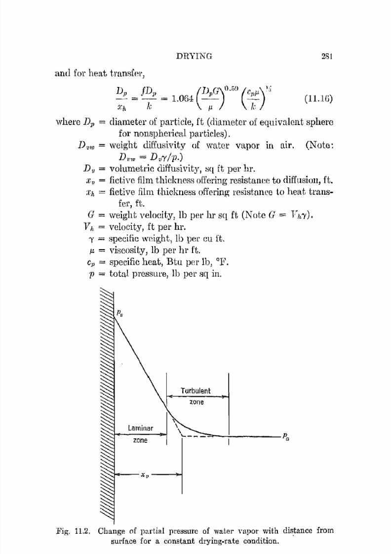
7/16/2019 Engenering Agriculture Perry
http://slidepdf.com/reader/full/engenering-agriculture-perry 293/422
DlWING 281
and for heat transfm,
Dp iD.p (DpG)n.5fl (Cp.JJ)':i- = - = 1.064 - - _
Xh k M kCIl.lo)
where D1' = diameter of particle, ft (diameter of equivalent spherefor nonspherical particles).
D1JIU = weight diffusivity of water vapor in. air. (Note:
D",. = Dv'Y/p,)Dv = volumetric dii'fusivity, Sf[ ft per hr.Xv = fictive film thickness offering resistan.ee to diffllSioIl, ft.
:t:h = fictive film thickness offering resistance to heat trans-fer, ft.
a = weight velocity, lb per hI' sq ft (Note C; = Fh'Y) ,
11" = veloeity, ft per hI','Y = specific weight, Ib per cu ft .
JJ = viscosity, lb per hI' ft.c1) = specific heat, Btu per Ib, OF.
P = total pressure, lb pel' sq in.
Turbulent
zone
X
Laminar \\
' "" ' I r - - ~ - P a
xv-jFig. 11.2. Change of partial presslll'C of water yupor with dis.tance from
surface for a constant drying-rate condition.

7/16/2019 Engenering Agriculture Perry
http://slidepdf.com/reader/full/engenering-agriculture-perry 294/422
282 AURICULTUR"\.L PROCESR ENGINEERING
The constant-rate drying period will procced until free moisture
d i R a l l p e : : t l ' ~ from the surface; the moisture removal rate will then
become progresflively less. The ll1oi:;,ture content at which thedrying rate ceases to bc constant is known as the critical moisture
content. No effective open moisture surfaces exist helow the
('ritical moisture content, and the (hying mechanism of the con
Htant-rate period no longer holds.1l.4. Falling.Rate Period. Pradieally all agril'ultul'al dry
ing takes placL' in the falling-rate period. Products that arc
moved into a drier from a washer may experience a shorL initial
constant-rate period. This period is usually minor when compared to the complete drying procc:os and can be neglected in the
calculations.
The falling-rate period is bounded by equilibrium moisturc
contents of an equilibrium moisture curve between zero and nearly
100 per cent relative hUl11idity. Moisture contents near the 100
pel' cent level would be in the constant-rate period. The 100 pel'
cent equilibrium puint is not a sntisfactory procedure for deter
mining thc exact critical moisLure content since cquilibrium moisture data observer1 abovc 95 per cent relative humidity are usu
ally unreliable.
U.5. The Falling-Rate Drying Mechanism. Drying in the
falling-rate period involves two processes, (1) movement of mois
ture within thc material to the surface and (2) removal of the
moisture from Lhe surface.
The internal m o i s t U l ' e ~ m o v e m c n t mechanism has been studied
by a number of investigators.6,8,11,15,17. 19 , 21
Finely divided materials containing cell or void cavities and
which are ebsentially not hygroscopic permit internal moisture
movement by capillary and gravitational flow. Moisture above
the saturation point in leather, ('otton, paper, etc., and above the
equilibrium moisture range in finely divided materials such as soil,
ceramic stock, paint, pigments, etc., moves by this mechanism.
Hygroscopi(' and non-hygroscopic materials dry comparably.
Moisture movement is by Liquid diffusion if the moisture con
tent is below the saturation point or within the equilibrium mois
ture range or if the material is a single-phase material such as
soaps, glues, and pastes. The movement is analogous to that of
heat conduction in a solid, and the following equations apply:

7/16/2019 Engenering Agriculture Perry
http://slidepdf.com/reader/full/engenering-agriculture-perry 295/422
DRYING
Within the solid
(1/.1) (oQ/aO) - Dvy(a.Mja:c)/lOOAt the surface
-D,fy(aMja;c) = 8(Ms - MEh
aj1,fjao = Dv(rJ2M/a:I;2)
(J = quantity of water, lb.
Dv = dii'fusivity, sq ft per hr.
y = dry-solid density, lb per Cll ft .
Al = moisture content, dry basis, per cent.
283
(11.17)
(11.18)
(11.19)
Ms = moisture content at surface, dry basis, per cent.ME = equilibrium moisture content at the relative humidity
of the drying air, dry basis, per cent.S = sm·face conductance, ft per hr.x = distance from center of the mass being dried, ft .
The llpplicability of these relationships has been studied by a
number of investigators.Solution of these equations was given by Newman S for a
mn,terial of constant diffusivity which dries without shrinking in
surroumEngs that provide a constant atmosphere and constant
surface conductance and leads to curveS similar to those for heat
conduction in solids (Figs. 9.2, 9.3, 9.4).ObservationR on large-size objects sunh as lumber have shown
that the observed moisture gradients through the unit differ from
those calculated from a constant diffusivity. The lack of coinci
dence is due to the fact that the diffusion coefficients vary with
moisture content, temperature, pressure) and material density, all
of which usually vary during drying.
The mechanism of moisture removal at the surface as set out
by Newman B is shown in equation 11.18. The moisture is as
sumed to be brought to the surface by diffusion and evaporated
to a vapor at the surface. The vapor is then removed from the
surface by conduction through the air film to the moving air. The
driving force is the difference in moisture content at the surfaceand the equilibrium moisture content of the material at the ail'
state.Experimental drying studies of agricultural products have
shown that the drying rate is proportional to the difference in

7/16/2019 Engenering Agriculture Perry
http://slidepdf.com/reader/full/engenering-agriculture-perry 296/422
28,1 AUmCULTURAL PROCESS ENGINEERING
moisture content between the material being dried aml the equi
librium moisture content at the drying ail' state or:
rIM/dl] = -a'(M - ME) (11.20)
Equation 11.20 is analogous to Newton's law of cooling, I t
cOllld be expected to hold quite well where the diffusivity of mois
ture within the solid is high ,,,ith respect to the surface conduc
tance and thiekneRs. Thi:-l is not t.rue for grains, fmits, and vege
tables, however, ,\"1lere a Ruh:'lLantial llloisture gradient exists
within the material during drying. The application to fruits and
grains is marle more plauf'Jihle by the artifice of replacing thedistributed internal rcsistance by a single lumped resistan(:e at
the surface, in series with the surface vapor resistance. The equi
librium moisture content that lllll::;t be postulated to secure a
linear plot of JI.I against 0, timE', on semilogaritlnuic coordinates is
often found considerably above the equilibrium values from hy
grostatic measurements at constant weight.
Additional limited tltudies havc indicntcd that air velocity nnd
temperature are probably relatc(1 to the drying rate, thm::
CI.' = aVnps (11.21)
where V = air rate, cu ft per (min sq ft).
ps = saturated water vapor pressure at the temperature of
the drying air, Ib per sq in.
The velocity exponent n is an indication of the relative effed of
internal diffu:;ion as compared to surface resistance upon the
drying rate. I f n is 0.6, there is no internal resistance to mois
ture movement, and resistance to vapor transfer nt the surface
controls the drying mte. Small values of n indicate that the in
tel'l1al resistance to flow controls the drying rate and that the
surface resistance is minor.
The saturated-pressure factor PH is included in the drying index
because the removal of moitlturc from lhe surfacc is a vapor
pressure mechanism, thus the driving force is proportional to tl1('
saturated pressure. The internal driving force may be considered as vapor pressurc in which case eM - lI1I!J) of equation 11.20
lllay he replaced with (rh - rhI!J) , the respective equilibrium rela
tive humidity values. This expression can be represented by
(liPs) (p - PE) in which JiI!J is the equilibrium vapor pressure
7/16/2019 Engenering Agriculture Perry
http://slidepdf.com/reader/full/engenering-agriculture-perry 297/422
DRYING 285
exerted by the material. This rational concept of the driving
force for drying is additional evidence snpporting the presence of
the P., terlYl in equation 11.21.Equations 11,20 and 11.21 when combined and integrated for
constant temperature, humidity, and vel(wity with limits give
(11.22)
JI,[0 is the initial a \'Crage moisture content at zero time; M 0' tile
average moisture content after a period of time e, The time (J is
usually expressed in hours,"
11.6. Heat and Mass Balance. Drying with heatN! air is an
adiabatic process, the energy for moisture evaporation being sup
plied by a reduction in temperature of the air. The \vet-bulb
(adiabatic humidification) lines of the psychrometric chart and
equation 11.20 represent this process and can be used i'01' calcu
lating a drying heat and mass balance.
Air of state ( I , Fig. 11.3, is heated to state b and passed through
tho material to be dried. The state point moves up the wet-bulb
line, and the air exhausts at. state d. The water transport rate is
v'W = - (Hd - I f h) (11.23)
v
where W = Wlttcr remov!\,ble rate, Ib per min.
V = air rate, eu I t per min per sq ft,
v = humid volume of ail' at point of rate measllrement,
el l ft per lb dry air.
The moisture removal rate from the drying-rate equation is
Wtl is the pounds of material (bone dry) per square foot through
whieh the air is passing. Therefore, the change in humidity is
. WdapsVt:J.H = lld - Hb = 1 (M - MB)
6000Y -nA
(11.25)
*Even though the above-mentioned drying-rata procedure is satisfactoryJOt' agricultural materials, the student should refllize that future rigorousst.udies may develop drying principles that will be more applicable generallyand some of the cUlTently acceptable approximations may become obsolete.

7/16/2019 Engenering Agriculture Perry
http://slidepdf.com/reader/full/engenering-agriculture-perry 298/422
286 AGRICULTURAL PROCESS ENGINEERING
Fig. 11.3. The ail' state chang!), b to d, foJ' a drying Pl'OCCRS. See alsoFig. 11.12.
The energy that must be supplied to he:1t the ail' can be foundwith the help of the psychrometric chart and is
60VA ()OVAq =- - (hb - It'l) =- - (tb - t,,)(O.2-t + 0,45H,,)
v v
q is the heat rate in British thermal units pel' hour for the air raterepresented by V.
The thermal efficiency in pel' cent may be exprei:ised as:
(11.26)
In this definition of thermal efficiency, which is commonly usedfor drying with hen.ted ail', the system is charged with the heatenergy of the fuel and is credited with the latent heat of
evaporation. The latent heat hIg
is at the exit temperature ofthe drying air.
An equivalent definition is the ratio of the ail' temperature dropin the drier to the rise in the heater. In drying with unheated
air, these definitions indicate an infinite efficiency i with mildheating, efficiencies above 100 per ceut may occur.
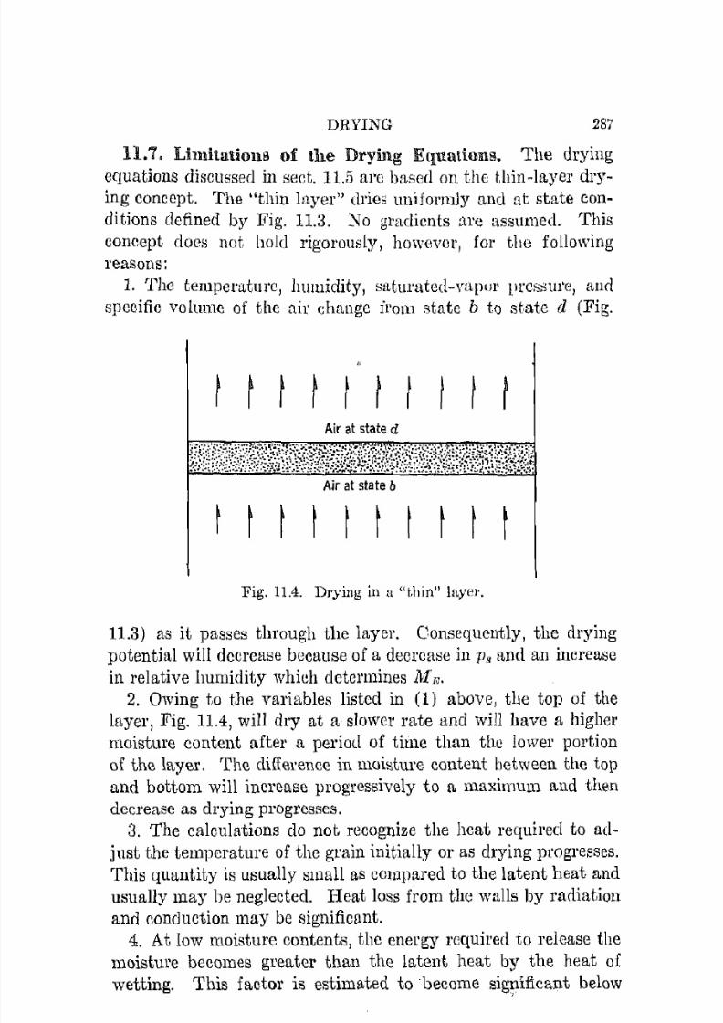
7/16/2019 Engenering Agriculture Perry
http://slidepdf.com/reader/full/engenering-agriculture-perry 299/422
DRYING 287
l l .7. Limitations of the Drying Eq.uations. The drying
equations discussed in sect. 11.5 arc based on the thin-!tlyer drying concept. The "thin layer" dries uniformly and at state con
ditions defined by Fig. 11.3. No gradients are assumed. Thisconcept does not hold rigorously, however, for the follO\vingreasons:
1. The temperature, humidity, S!1turuted-vtl[1ol' preS:lUrc, andspecific volume of the air ehange from state b to state d (Fig.
Air at state d
Ajr at state b
t t t ttt tt t
Fig. 11.4. Drying ill a "thin" layer.
11.3) as it passes through the layer. Consequently, the dryingpotential will decrease because of a decrease in P8 and an increase
in relative humidity which determines ME.2. Owing to the variables listed in (1) above, the top of the
layer, Fig. 11.4, will dry at a slower rate and will have a highermoisture content after a period of tiine than the lower portion
of the layer. The difference in m o i ~ t u r e content between the topand bottom will increase progressively to a Inaximum and then
decrease as drying progresses.3. The ealculations do not recognize the heat required to ad
just the temperature of the grain initially or as drying progresses.This quantity is usually small as compared to the latent heat and
usually may be neglected. Heat loss from the walls by radiationand conduction may be significant.
4. At low moisture eontents, the energy required to release the
moisture becomes greater than the latent heat by the heat of
wetting. This factor is estimated to become sigrificant below
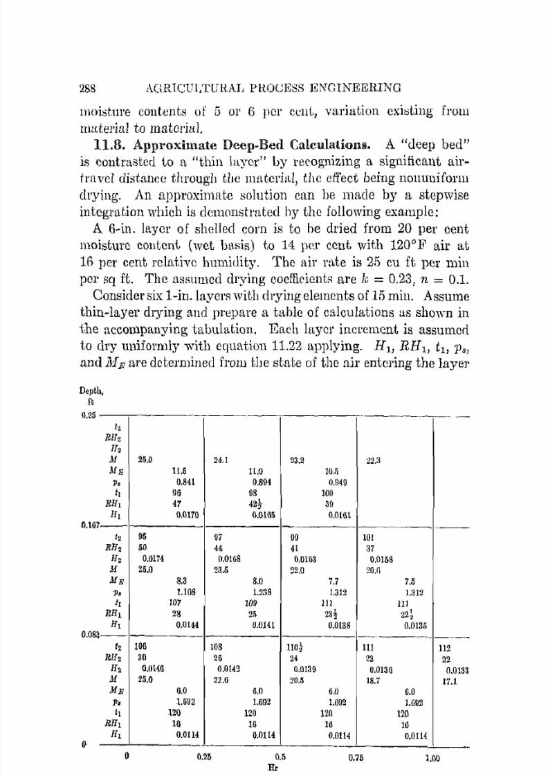
7/16/2019 Engenering Agriculture Perry
http://slidepdf.com/reader/full/engenering-agriculture-perry 300/422
288 AGRICULTUltAL PltOCESS ENGINEERING
moistme contents of 5 01' 6 pCI' cenL, variation e x i ~ t i n g frOll!
material to material.11.S. A}lproxhnate Deep-Bed Calculations. A "deep bed"
is eOlltrasted to a "thin layer" by recognizing a significant ai1'
travel distance through tllC material, the effect being nOIluniform
drying. An approximate solution can be made by a stepwise
integration which is demonstrated by the following example:
A 6-in. layer of shelled corn is to be dried from 20 per cent
moisture content (wet basis) to 14 per cent with I20°F air at
If) per cent relative humidity. The air mt,e is 25 cu ft per min
per sq ft. The assumed drying coefficients are k = 0.23, n = 0.1.
Consider six I-in.laycl'fl with drying elements of 15 min. Assume
thin-layer drying and prepare a table of calculations as shown in
the accompanying tabulation. Each layer increment is assumed
to dry uniformly with equation 11.22 applying. HI' RH1, t l , 1)8,
nnd ME are determined from the state of the [til' entering the layer
Deptb,I t
0.25
0.101
0.083
I}
12
R1l2
Il2M
lifE
p,
II
RIll
If l
/2
RIf2If2MMEp,
ItRlli
If ,
12
RII2
112
MMEf1.
II
Rill
lit
25.0
95
50
0.0174
25.0
lOG
30
0.0146
25.0
o
24.1
11.5
0.84190
47
0.0170
97
44
0.0158
2a.5
8.3
!.l08
107
28
0.0144
108
260.0142
22.0G.O
1.002
12016
0.0114
0.25
-
11.0
0.894
98
42!0.(1165
8.0
1.238
109
25
0.0141
6.0
1.092
120
16
0.0114
0.5
Hr
---------
23.2 22.:1
10 •
0.940
100
39
0.0161
- - -99 101
41 37
0.0103 0.0158
22.0 .20Ji
7.7 7.5
1.312 1.:112
111 I I I
23! 22;
0.0138 0.0135
. _ - - - - - - - -no} 111 11224 23 22
0.0139 O.Q130 0.0133
20.5 18.7 17.16.0 0.0
1.692 1.092
120 12016 16
0,0114 0.0114
0.75 1.00
7/16/2019 Engenering Agriculture Perry
http://slidepdf.com/reader/full/engenering-agriculture-perry 301/422
DRYING 289
increment and represent the average for the time increment shown.
111 is the avcrage initin.l moisture content for the layer at the time
shown. H 2 , RH2, and t2 are stute conditions for the air leaving
the layer at the time shown. The air entering the grain has a
temperature of 120°F and a relative humidity of 16 per cent.
These values establish the psychrometric adiabatic humidification
line upon which the air state moycs as drying progresses.
The calculated average moisture content of the bottom layer
after, for example, Y:J hI' of drying is 20.5 per cent. The char
acteristics of the air leaving the bottom layer and entering the
second layer are found by calculating the humidity increa,sc in the
air by equation 11.25. The increase added to 0.0114 is 0.0142.
The later vnlue H2 is applied to the psychrometric adiabatic line
from whieh values of RH2 and t2 are taken. HI' RH1 , and t l , for
the second layer, are respective averages of the subscript-2 values
for the air leaving the lower layer at the beginning and end of
the period. The saturated pressure 1.238, is that at t l • J1fE
istaken
from Fig. 11.1 forRH
1,
or 8 per cent.The
calculationsfor the second layer progress from left to right, Ps and RHl chang
ing for each time calculation.
The above procedure can be extended both as to depth and time
until the desired operating range is eoverec1. The errors discussed
previously can be minimized by using small increments of time
and depth.*
DRYING PROCEDURES
Agricultural materials must be dried by different procedures
because of their inherent characteristics which may be classified
on the basis of the following factors:
1. Ternperature Tolerance. High temperatures may reduce
germination, partially cook the product, 01' ehange its dlemical
or physical characteristics.
2. Humidity Response. Materials that undergo physiological
or other change during drying, e.g., tobacco, lumbcr, prunes, may
have to be dried with air of a specific moisture content.
*The errors can be further minimized by nn appropriate numerical Pl'O
cedure such as the first modification of Euler's method. See J. B. Scarborough, N ~ l m e r i c a l JvIathematical Analysis, The Johns Hopkins Press, 1930.
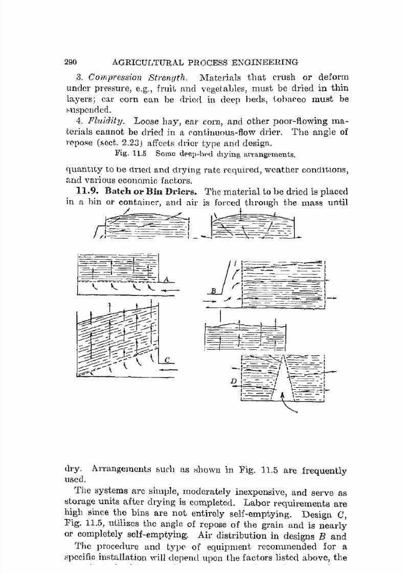
7/16/2019 Engenering Agriculture Perry
http://slidepdf.com/reader/full/engenering-agriculture-perry 302/422
290 AGRICULTURAL PROCESS ENGINEERING
3. Compression Stl'enuth. Materials that crush or deform
undcr pressure, e.g., fruit and vegel aLles, must be dried in thin
layers; car corn can he ({ried in deep heds, tobaeco must be
l-uspcnded.
4. Fluidity. Loose hay, ear com, and other poor-flowing ma
terials cannot be dried in a continuous-flow drier. The angle of
repose (boct. 2.2:3 ) affects drier type and design.
The procedure and type of equipment recommended for a
~ j ) e c i f i c installation will cleprml upon the factors listed above, the
quantity to be dried and drying rate required, weather conditions,and various economic factors.
1l.9. Batch 01' Bin Driers. Thc material to be dried is placed
II I a bin 01' container, and air is forced through the mass until
dry. Arrangements :;uch as H110Wll in Fig. 11.5 are frequentlyused.
The systems are ::;ill1ple, moderately inexpensive, and serve as
storage units after drying is completed. Labor requirements are
high since the bins are not entirely self-emptying. Design 0,
Fig. 11.5, utilizes the angle of repose of the grain and is nearly
or completely self-emptying. Ail' distribution in designs Band

7/16/2019 Engenering Agriculture Perry
http://slidepdf.com/reader/full/engenering-agriculture-perry 303/422
DRYING 291
D is not uniform. Consequently, nonsYll1mctl'ical drying mayresult.
Materials to be dried by this system must have sufficient compressive l'esist[mce to resist crushing under load and to maintainthe normal void space so that
proper ail' rates ean be maintained.Resistance to air flow limits the
depth for highly resistant materials
since adequate nil' rate!'; are p o ~ sible unly with excessively large
power units.The ll1ass dries progrel:'::;ivdy in
the direction of air flow. The part
of the mass in the uir discharge region is subject to high humidities
und moderate temperatures and
may spoil from mold before the
moving drying front hl\S reached it.
Adequate drying of the mass in theair discharge region is accompa
nied by overdrying uf the mass in
the air cntrance region. This un
desirable feature can be minimized
by (1) drying with the lowestpracticable ail' temperature, (2)
using the highest practicable air
rate, and (3) transferring the 11Ul
tel'ial to another bin when the
average moisture content for the
mass is that desired; the mass
must be mixed uniformly when Fig. 11.6. The column drier.
moved.The performance can he estimated by the d e e p ~ b c d procedure
of sect. 11.8.11.10. Continuous Gravity-Flow Driers. Granular materials
that flow readily, permit air to flow through them, ane! arc notdamaged in handling, can be dried in a g r a v i t y ~ f t o w drier such
as the column drier of Fig. 11.6. The wet material is placed in
the hopper and flows by gravity between the perforated retaining
walls and is discharged at the bottom by a continuously operating

7/16/2019 Engenering Agriculture Perry
http://slidepdf.com/reader/full/engenering-agriculture-perry 304/422
292 AGRICULTURAL PROCESS ENGINEERING
metering vulve. Heated air is forced across the column at right
angles to the direction of grain motion. The column may be in
dined to simplify construction or fitted with baffies to stir the
ll1ftSS us it progresses through the drier. Many designs are used,
but the principle of operation in all case:> is that of Fig. 11.6.
The continuous gravity-fiow drier is moderately expensive par
ticularly when the mt,terials-handling equipment required must
Le charged to it. High buildings are usually required to house
it because height is required to get capacity. I t is, however, a
most acceptable device where large capacities and long-season use
are characteristics of the operation. Labor costs are low sincehandling is completely mechanieal.
The capacity is directly proportional to thc column width and
material movement ratc through thc column. The retention time
in the column is the drying time for the material as defined by its
drying indiees, the required moisture reduction, and state factors
of the drying air. Since the retention time is fixed for each l n d i ~vidual situation, drier capacity is proportional to height.
Column-drier performance may be estimated by the d e e p ~ b e dprocedure. Note that the example, sect. 11.8, is for conventional
column-drier performance. I f the column of grain is stirred as it
moves, the t h i n ~ l u y e r procedure may be used with acceptable
accuracy.
11.11. Rotary Driers. Materials that are not free flowing
and that are not damaged by continuous handling are usually
dried in Totary driers. Chopped forage, fruit and vegetable resi
dues to be dried for livestock feed, and fertilizer components areexamples of materials dried in this manner.
The rotary drier has a high initial cost and requires more floor
space per unit of capacity than either the 'batch or column drier.
Consequently, it should not be used if the batch or column drieris suitable.
Agricultural rotary driers such a ~ shown in Fig. 11.7 are direct
fired and single-, double-, and triple-drum types. The multiple
drum types are prcferred since the over-all length can be short;and heat losses by conduction and radiation small.
The inside of the drum may be fitted with flights that lift the
material and shower it down through the heated air. Flight
design varies with the material to be dried. Chains or other
dividing devices may be fitted to the inside of the drum to divide

7/16/2019 Engenering Agriculture Perry
http://slidepdf.com/reader/full/engenering-agriculture-perry 305/422
DRYING
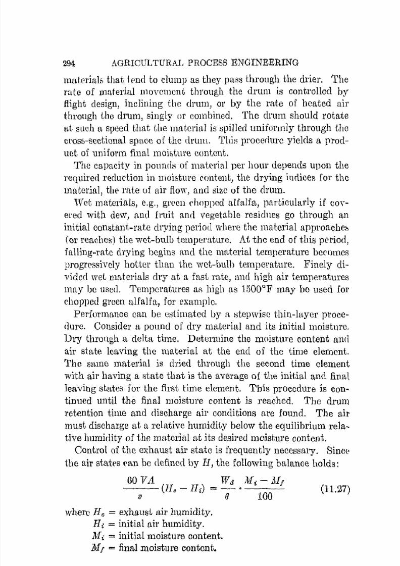
7/16/2019 Engenering Agriculture Perry
http://slidepdf.com/reader/full/engenering-agriculture-perry 306/422
294, AGRICULTURAL PROCESS ENGINEERING
matcl'ialE> that, i cnd to clull1p as they pass through the drier. The
rate of material l1l0vemcnt through the drum is controlled by
flight design, inclining the drum, or by the rate of heated air
through the drum, singly or combined. The drum should rotate
at such a speed that the material is Hpilled uniformly through the
crOSb-sectional space of thc drulll. This procedure yields a prod
uct of uniform final moisture. contcnt.
The capacity in pounds of mn,terial pel' hour depends upon the
required reduction in moisture ('ontent, the drying indices for the
ll1ateritll, the l'nte uf air flow, and size of the drum.
Wet materials, e.g., grpen chopped alfalfa, particularly if cov
ered with dew, and fruit and vegetable residnes go through an
initial constant-rate drying period where the material approaches
(or reaches) the wct-bulb temperature. At the end of this pcriod,
falling-r!1.tc drying begins and the material temperature becomcs
progressively hotter than the wet-bulh temperature. Finely di
vided weL materials dry at a fast rate, und high air temperatures
maybe used.
TemperaturesaR high
as1500
Q
Fmay be
used forchopped green alfalfa, for example.
Performance can be e::;timatcd by a stepwise thin-layer proce
dure. Consider a pounel of dry material and its initial moisture.
Dry throllg,h a delta time. Determine the Il10isture content ane!
air state leaving the material at the end of the time element.
The same material is dried through the second time element
with air having a state that is the average of the initial and final
leaving states for the first time element. This proccdure isc o n ~
tinued until the final moisture content is reached. The drum
retention time and discharge air conditions are found. The air
must discharge at a relative humidity below the equilibrium rela
tive humidity of the material at its desired moisture content.
Control of the exhaust air state is frequently necessary. Since>
the air statE's ran be defined by II, the following balance holds:
GO VA Wd Afi - M,v (He - Hi) = e- . 100
where He = exhaust air humidity.
Hi = initial ail' humidity.
M = initial moisture content.
Mr = final moisture content.
(11.27)
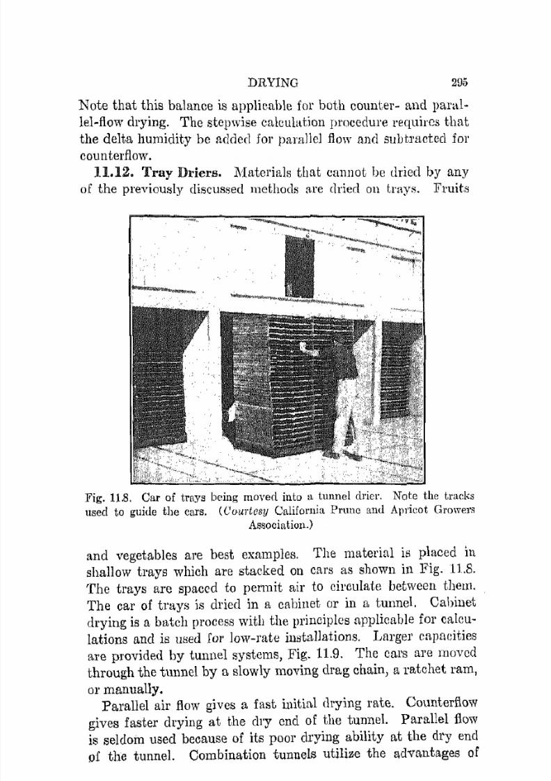
7/16/2019 Engenering Agriculture Perry
http://slidepdf.com/reader/full/engenering-agriculture-perry 307/422
DRYING 295
Note that this balance is applicable for both counter- and paral
lel-flow drying. The stepwise calculation procedure requires that
the delta humidity be added for parallel flow and subt.racted for
counterflow.
11.12. Tray Dl'iers. .Materials that cannot be dricd by any
of the previously discussed methods (11'e dried on tmys. Fruits
Fig. 11.8. Car of trays being moyed into a tunnel dl'icl·. Note the tracksused to guide the cars. (C'(}urtcsy California Prnne and Apl'ieot Growers
Association.)
and vegetables are best examples. The material is placed in
shallow trays which are stacked on cars as shown in Fig. 11.S.
The trays are spaced to permit air to circulate between them.
The car of trays is dried in a cabinet or in n tunnel. Cabinet
drying is a batch process with the principles applicable for calcu
lations and is Heed for low-rate installations. Larger capacities
are provided by tunnel systems, Fig. 11.9. The cars are movcd
through the tunnel by a slowly moving drag chain, a ratchet ram,
or manually.Parallel air flow gives a fast inithtl drying rate. Counterflow
gives faster drying at the dry end of the tunnel. Parallel flow
is seldom used because of its poor drying ability at the dry end
of the tunnel. Combination tunnels utilize the adv(1.ntages of

7/16/2019 Engenering Agriculture Perry
http://slidepdf.com/reader/full/engenering-agriculture-perry 308/422
296 AGlUCULTURAL PROCESS ENGINEERING
hol,h parallel flow and counterflow, but the initial cosi is greater
and control if:, more difficult. Counterfiow tunnels are most ex
tensivelv lIseel. The air rate must be high enough so that therelative' humidity of the discharge air is below the equilibrium
relative humidity of the ma,tcrial at the point where the material
dis clutl'ges.Performance can be estimater! by the pro('eclul'e of rotary driers j
a car and its contents is w-,ell as the unit of calculation. N otc
that the humidity change of the air clue to the removal of mois
ture from the material is positive for parallel fluw and negative
Fresh ~ - - - - - ~ ~ - - - - - , ! . . ; ! ! . ! - - : : > - - - - - - - - - - ,air ~- - - ~ - _ _ _ . . . -\\ \ ~ - - - - - ~ ~ - - - - - - ~ - - ~ - - - - - - \
\
I"lg. 11.9. Plan of a tunnel drier. The cars move from ]pft to right forcountedlow operation, from right to left for parnllel flow.
for counterflow. The material-charging end is used as a reference
in both cases.
11.13. Spray Driers. Spray driers remove the water fromsolutions or suspensions and dry the resulting powder to a mois
ture content that approaches equilibrium with the exhaust drying
air. Spray driers arc used extensively in the food, chemical, and
pharmaceutical industries.Design varies from a rectangular chamber fitted with spray
jets, through which the drying air passes to continuous large
volume systems such as Fig. 11.10. Three procedures are usedfor breaking the material into fine (h·ops.
1. High-Pressure Atomization. The liquid is forced through a
nozzle under high pressure. Mixing with the drying air and the
spray pattern can be controlled. Drop size and gradation are
difficult to predict. Nozzle life is short when abrasive materialsare sprayed.
2. Centrifugal. The liquid is fed at low pressure onto a hori
zontal disc or cup turning at speeds up to 20,000 rpm or more.
The material breaks up into small drops as it leaves the edge of

7/16/2019 Engenering Agriculture Perry
http://slidepdf.com/reader/full/engenering-agriculture-perry 309/422
II
-
DRYING 297
--

7/16/2019 Engenering Agriculture Perry
http://slidepdf.com/reader/full/engenering-agriculture-perry 310/422
298 AGRICULTURAL PROCESS E ~ G I N E E R I N Gthe rotur. The drops are of uniform size, and materials not suitable for nozzleti can be dried. Air-liquid drop mixing may be
Entrainmentseparationchamber
Enlargedvapor tube
R tu rn tu be forrecovered milk
Milk solidsretu rn ing toevaporator
Flash prooftangentmilk inlet
Condensationoutlets
Individually operatedstreamlined coilsalternating directionof steam flow
For creating andmaintaining a vacuum:double-stage ejectorwith Intermediatecondenser
Water inlet
Turbine-ormotor-driven
water-dischargepump
Fig. 11.11. Vacuum pan with cntnlilllllclli. separation chamber and counter
('11rrent condenser used for milk con('cntration. ((,'llurll'sll Arthnr HarriH
and Co.)
poor since the drops follow an umbrella-shaped trajectory. Discrotor and bearing maintenance are high.
3. Two-Fluid Atomizing. Air or steam under pressure breaksthe liquid into fine drops by a mechanism comparable to that of

7/16/2019 Engenering Agriculture Perry
http://slidepdf.com/reader/full/engenering-agriculture-perry 311/422
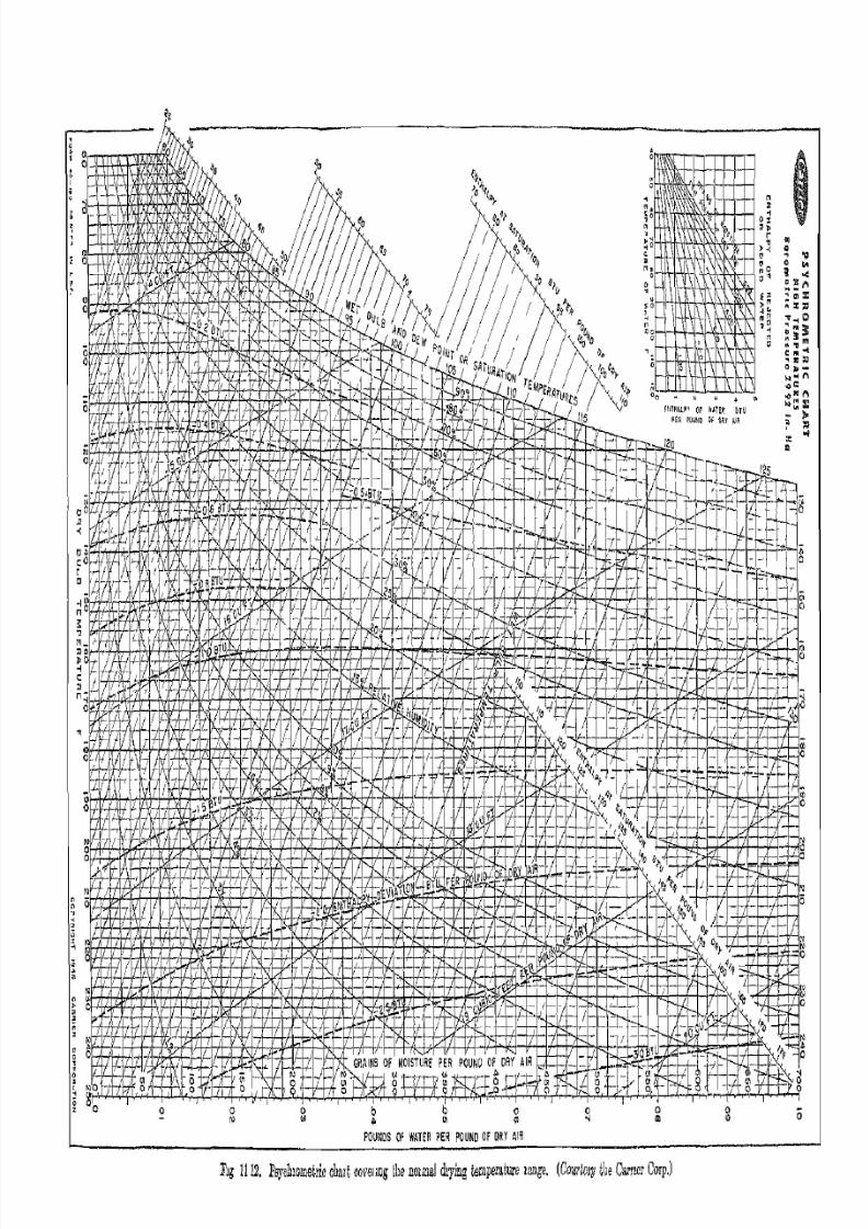
7/16/2019 Engenering Agriculture Perry
http://slidepdf.com/reader/full/engenering-agriculture-perry 312/422
A i T r ~ ' gb •
R OUND OF DR Y AIR
POUNDS OF WATtR PE (Courtcsy the Carner Corp,)
d ' t mperaiure lange,- - ~ ."'., OV811Ug Ihe nOlma! Iymg e-___ Fig 1112, PsyehlOmelrlC chari c

7/16/2019 Engenering Agriculture Perry
http://slidepdf.com/reader/full/engenering-agriculture-perry 313/422
7/16/2019 Engenering Agriculture Perry
http://slidepdf.com/reader/full/engenering-agriculture-perry 314/422
DRYING 20()
paint sprayerH. Operating costs are high. This I:lyt-:tem io; u:"ed
only for the lllost difficult atomizing johs and experimental units.
BecaUi:,e of the small diameter of the rlropli, drying is {'xtremely
fast and the material is dry when it I"paehC'R the walls or hottom
of the container.
11.14,. Concentrators. Coneentl'aton;, also ('aIled C'vapn
"ators, are m;pd to concentrate milk, fruit and vegl'tablp jui(·cs.
jamR and jellies, etc., by boiling off a purtion of the watC'l". Be
eUUi:ie of the conditions of operation, the concentrator is frequently
called a vacuum pan. A "pan" shown in FiV;. 11.11 ,. is operated
under a partial vacuum because (1) low-boiling tell1jlcrat1ll"es do
not damage heat-sensitive materials and (2) a large tCHll)eraturc
difference is maintained between the steam and boiling liquid
which permits a high heat-transfer rate.
The water spray condenses the water vapor remove(l from the
('oncentrating liquid. The boiling temperatnrc of the liquid being
concentrated is controlled by the temperature of the water-con
densate mixture leaving the condenser. The water-condensate
mixture is removed by a pump or barometric leg. The vacuum
is usually maintained by a steam ejector, although a -vacuum
pump may be used. Since the condenser handles the vapor from
the concentrating liquid, the ejector needs to handle only the non
condensable gases and air from leaking gaskets.
The steam coils arc usually fed with steam at 5 to 10 Ib per
sq in . The hailing is extremely vigor OUR hecause of the high telll
perature difference. Thus, a high heat rate is possible with mini
mum heat exchange surface and a "cooked" flavor is improbable
owing to 1.he surface speed" of the liquid.
This unit can operate on a batch basis or continuously by
means of a suitable pump that continuously removes liquid from
the bottom of the "pan" and by continnouR feeding in of the liquid
stock.
REFERENCES
1. Comings, E. W., and Sherwood, T. K The Drying of Solids, VII.Moisture Movement by Capillarity in Drying Granular Solids. Ind.
and Eng. Chern. 26:1096-98. 1934.
*This is only one of a number of designs which vary from compahy to
company and for material to material.

7/16/2019 Engenering Agriculture Perry
http://slidepdf.com/reader/full/engenering-agriculture-perry 315/422
300 AGRICULTURAL PROCESS ENGINEERING
2. C}amson, D. 'V., Thodos, Ct., and Hougen, O. A. Heat, Mass, andMomentum Transfer in the Flow of Gases Through Granular Solids.
TraIls. Am. Inst. Chern. EU(Jrs. 39 :1--35. HN3.3. Gilliland, E. R., and Sherwood, T. Ie The Drying of Solids, VI. Dif
fusion Elluations for the Period of Constant Drying Rate. Ind. and
Eng. Chern. 25:1134-36. 1933.4. Henderson, S. M. A Basic Concept of Equilibrium Moisture. Agr. Eng.
33 :29--32. 1952.5. Hlynka, F., et al. A Comparative Study of Ten Electrical Meters for
Determining Moistme Content of Wheat. Canadian J. Reseanh27:382-397. 1949.
6. Hougen, O. A., McCauley, H . • ., and Marshall, W. R., Jr . Limitations
of Diffusion Equations in Drying. 'l'rans. Am. Inst. Chern. Engr.
36:183-209. 1940.7. Marshall, W. R.., Jr., and Hougen, O. A. Drying of Solids by Through
Circulation. Tl·ans. Am. Inst. Chem. Engr. 38 :91-121. 1942.
8. Newman, A. B. The Drying of Porous Solids. Diffusion and SurfaceEmission Equations. Trans. Am. I n . ~ t . Chern. En(]r. 27 :203-310. 1931.
9. Official and Tentative 1vlethods (/f Analllsl:s of the As.sociation of Official
A(wicultzmd Chemists. Published by the Association of Offichl Agri
cultural Chemists, P. O. Box 540, Benjamin Franklin Station, Washington, D. C.
10. Perry, R. L., p.i; aJ., Fruit Dehydration. 1. Prineiples and Equipment.
Californiet AUT. Exp. 81.n. Bull. 698. 1946.
11. Perry, R. L. Heat and Vapor Transfer in the Dehydmtion of Prunes.
'l'rans. AB.M.E. 66 :447-456. 1944.
12. Seltzer, E., and S e t t e l r n e ~ ' e r , J. T. Spray J)j1Jing of Foods. Advances in
Food Research, Vol. 2. Pp. 399-520. Academic Press. 1949.
13. Shedd, C. K. Mechanical Drying of Corn on the Farm. U.S.D.A. Cin.
839. 1950.
14. Sherwood, T. K. The Air Drying of Solids. Trans. Am. Inst. Chem.
Engr. 32 :150-68. 1936.15. Sherwood, T. K The Drying of Solids, II. Ind. and En(]. Chem.
21 :976-980. 1929.
16. Sherwood, T. K. The Drying of Solids, III. Mechanism of the Drying
of Pulp and Paper. Ind. and En(]. Chem. 22:132-36. 1930.
17. Sherwood. T. K. The Drying of Solids, IV. Application of Diffusion
Equatiolls. Ind. and Eng. Chem. 24:307-310. 1932.
18. Sherwood, T. K, and Comings, E. W. The Drying of Solids, V.
Mechanism of Drying of Clays. Ind. Clnd En(]. Chem. 25:311-16.
1933.
1!1. Van Arsdel, W. B. Approximate Diffusion Calculations for the FallingRate Phase of Drying. Chem. Eng. Proor. 43: 13-24. 1947.
20. Von Loesecke, H. W. Drying and Dehydration of Foods. Reinhold.
1943.
21. Weisselberg, A., and Olive, T. R. Principles and Practices in Drying
Solids. Chem. Met. Eng. 49:93-102. 1942.

7/16/2019 Engenering Agriculture Perry
http://slidepdf.com/reader/full/engenering-agriculture-perry 316/422
DRYING 301
PROBLEMS
1. 60,000 lb of shelled corn at 22 pCI' ceni moisture conjpnt (wet h a ~ i s ) are
to be dried to 13 llel' cent moisture ('ani ('nt. Dl'terUlille:
a. The dry-basis moisture contents.b. The amount of dry material.
c. The gallons of wal er to be removed.
2. A thin layer of material dried with air of llO°F dry bulb and 80°F wetbulb had moistUl'e contenls [1t 2-hl' intervals (dry basis) as follows:
30.0, 22.0, 17.3, 11.6, 13.1, and 12.2.
a. Determine the drying COllRt::mL a' and the apparent equilibrium mois
ture content of approach.b. How much time would be required to dry il'om 20 to 12 per cent (dry
basis) with 110°F air? with 140°F air? Assume an eljuilihrium moisture content of 10 per cent (dry basis) and the same ail' rate as in (a).
3. A steel bin 14 fL in diameter and 8 ft deep contains grain sorghum
which must be dried from 18 to 14 per cent (wet basis) moisture content.The floor is perforated, and air moves vertically through the mass at
2 eu ft per min per bu. Unheated 75°F air with a 55°F dew point is usedfor drying. I f the average discharge air temperature is 66°F, how manyhours will be required to dry the grain?
4. Develop a drying pattern simibr to that of sect. 11.8 for an air rate of100 cu ft pel' min and initial temperature of 160°F, the initial humiditybeing the same as that of the example.
5. Eggs are to be spray dried to 5 per cent (wet basis) moisture content.
Air initially at 70°F dry-bulb temperature and 60°F wet-bulb tem
perature is heated to 250°F.
a. What is the lowest possible discharge air temperature?
b. How many British thermal units of heat must be supplied to the airper pound of moisture removed if the air discharges at 195°F?
U. A rotary drier uses 70·F, 36 per cent relative humidity air. I t is heated
to 250°F and discharges at 120°F. What per cent of the fuel might be
saved if the latent and sensible heat in the discharge air were used to
assist in heating the incoming ail'?7. A tunnel dehydrator (Fig. 11.9) operates with a wet bulb controlled at
115°F. Outside air at 70°F and 60°F wet bulb is heated to 160°F.
The ai r is discharged at 140°F. What per cent of the air must be
recirculated?8. Derive equation 11.3.
7/16/2019 Engenering Agriculture Perry
http://slidepdf.com/reader/full/engenering-agriculture-perry 317/422
CHAPTER 12
I\et'l'igel'ation
NOMENCLATURE
A = evaporator heat-exchanger area, sq ft .
c = specific hmtt, Btu per (OF Ib).
D = piston displacement, cu ft per l"evolutioll.
Eo = compression thermal efficiency, per cent.
E" = compressor volumetric efficiency, pel' cent.lIa = heat content, va]JOI' entering compressor, Btu pel' lb.III, = he1tt, content, vapor leaving compressor, Btu per lb.
he = \tl'lLt I1lmtent, liquid entering evaporatOl", Btu per lh.
hi, hI' = heat content, wet evltPorating liquid, Btu per lb.fig = heat content, saturated vapor Itt evaporating pressure, Btu
per lb.hg , = heat content, Huperheated vapor at evaporating pressure, Btu
perlb.
N = number of pistolls.q = heat, rate, Btu per hr.
To = I1bsolute temperature of eVl1porating liquid, OR.
TH = absolute temperature of condensing liquid, OR.
tl = temperature of medium before cooling, OF.
t2 = t.emperature of medium after cooling, OF.
ta = llvaporating refrigerant temperature, OF.
U = heat-transfer (loeffieient, Btu per (hr sq It OF).
Vg = specific volume of refrigerant vapor, eu ft per lb.
WI, W2, Wr = refrigerant rate, Ib per hr.JV", = maRS rate, cooling medium, Ib pel' hr.
Refrigeration may be defined as the process of removing heat
from a body that is below the temperature of its surroundings.Or refrigeration may be defined as the process of transferring heat
energy from a lower to a higher temperature. Natural refrigera
tion is that produced by the use of natural icc. Mechanical refrigeration is that accomplished by means of refrigerating engineswhich operate on thermodynamic principles.
12.1. Natural Refrigeration. Ice is satisfactory as a re
frigeration medium for temperatures down to approximately 40°F302

7/16/2019 Engenering Agriculture Perry
http://slidepdf.com/reader/full/engenering-agriculture-perry 318/422
REFRIGERATION 303
under such conditions as (1) shurt annual refrigeration periodfo,
(2) duty away from power sources, and (3) where the ice cost is
nominal. Temperatures below 32°F may be prorluced by mixingfinely divided ice and varioHt' chemicals some of which are given
in Table 12.1.
Table 12.1 TEMPERATURE OF ICE-FREEZING MIXTUREtl
ChemiralNaCLCaChHNOa (dilute)KOHHNOa (trace H2S04)
Pel" C'etd ofChemical in
lIfixturc,
by Weight2/i(\0
50fi750
Temperature,
o f
-1.( ;
-27.1\
-a1.0-38.a-40.0
The latent heat of ice is IJ4 Btu per lb, and its specific heat is
0.47 Btu per 1b pel' of. The cooling rate is dependent upon the
temperature difference and method of air or Wl1ter circulationover it. Where ice is used for cooling recirculating water, it is
difficult to secure water krnperaturcs IJclow 39°F if thc ice hi
floating in a tank, because tho maximum dcnfoity of water is
rcuehed at 39°F and circulntion within the tank is poor. A showel·
of return water over unsubmerged blocks of ire on a rark is much
more cffcctive than a tank.
12.2. Mechanical Refrigeration. Refrigcration processes
using mechanical devices and electrical 01' other energy are canedmechanical refrigeration systems. Two broad classifications are
(1) absorption and (2) vapor compression systems. The vapor
compression sYfltems are the more common an(l will lw discussed
in this chapter.
The operation of the vapor compression l:;y::.tem is shown
schematieally in Fig. 12.1. The liquid refrigerant in t.he receiver
or supply tank is under high pressure. Because of this pressure
the liquid is forced through the liquid line to and through theexpansion valve into a region of low pressure produced by the
compressor. The liquid refrigerant evaporates or boils to a vapor
in the evaporator. The heat required for evnporation comes from
the surroundings, and cooling results, The vapor moves at low
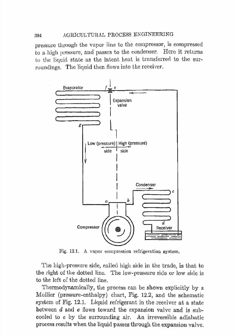
7/16/2019 Engenering Agriculture Perry
http://slidepdf.com/reader/full/engenering-agriculture-perry 319/422
304 AGRICULTURAL PROCESS ENGINEERING
pressure through the vapor line to the compressor, is compressed
to a high pressure, and passes to the condenser. Here it returns
to the liquid state as the latent heat is transferred to the s u r ~roundings. The liquid then flows into the receiver.
(
Evaporator
g__ J
..... --I xpansionvalve
III
Iow ( p ~ s s u r e ) I ighJpressure)
side side
II
III
L __ 2.Cl:.r-il b
J :
Comp"""
Gd
Condenser, . . . . ; ; ; = ~ - - - - . . c
dReceiver
1--====::= =1Fig. 12.1. A vapor compression refrigel'ation system.
The high-pressure side, called high side in the trade, is that to
the right of the dotted line. The low-pressure side or low side is
to the left of the dotted line.
Thermodynamically, the process can be shown explicitly by a
MollieI' ( p r e s s u r e ~ e n t h a l p y ) chart, Fig. 12.2, and the schematicsystem of Fig. 12.1. Liquid refrigerant in the receiver at a state
between d and e flows toward the expansion valve and is s u b ~cooled to e by the surrounding air. An irreversible adiabaticprocess results when the liquid passes through the expansion valve.

7/16/2019 Engenering Agriculture Perry
http://slidepdf.com/reader/full/engenering-agriculture-perry 320/422
REFRIGERATION 305
The state changes from e to f, a part. of the liquid flashing to n
gas. The portion flashing is
(12.1)
The wet mixture f evaporates to a state g' between g and a in the
evaporator where the useful cooling takes place. The vapor
further superheats to sLate a as it is eondneted to the compressor.
It
Fig. 12.2. The vapor c o m p r c s ~ i o n mechanical refrigeration process, given
ReliematicnUy, by 11 Mollie!" (pressure-enthalpy) chart.
The gas is compressed isentropic ally by the compressor from a to
b. The hot compressed gas is desuperheated to c and condensed
to a liquid by removing the latent heat Ly the condenser, thus
reaching point d. The liquicl is usually subcooled to a point ein the condenser or by ambient air exchange.
The useful cooling or refrigeration prj" pound of refrigerant il-l
(12.2)
The power required by the compressor per pound of refrigerant is
ha - ha, which is the mechanical equivalent in terms of Btu. The
coefficient of perfonnance is a factor that designates the number
of useful Btu of cooling capacity per equivalent mechanical Btu
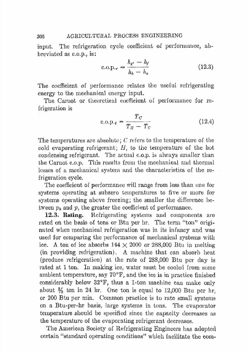
7/16/2019 Engenering Agriculture Perry
http://slidepdf.com/reader/full/engenering-agriculture-perry 321/422
306 AGRICULTURAL PROCESS ENGINEERING
input. The refrigeration cycle coefficient of periOl'llHUICe, ab
breviated as c.o.p., is:
(12.3)
The coefficient of performance relates the useful refrigerating
energy to the Ulechanical energy input.The Carnot or theoretical eocfIicient 01 performance for re
frigeration is
Tc
c.o.p.t = ---TlJ - Tc (12.4)
The temperatures are absolute; C refcrs to the temperature of the
cold evaporating refrigcrant; IJ, to thc temperature of the hotcondensing refrigerant. The actual c.o.p. is always smaller thanthe Carnot c.o.p. This results from the mechanicnl and thermal
losses of a mechanical system and the characteristics of the re
frigeration cycle.
The coefficient of performance will range from less than one forsystems operating at subzcro tcmperatlll'es to five 01' more for
systems operating above freezing; the smaller the difference be
tween Ph and p, the greater the coefficient of performance.12.3. Rating. Refrigerating systems and components are
rated on the basis of tons or Btu per hr. The term "ton" originated when mechanical refrigeration was in its infancy and was
used for comparing the performance of mechanical systems with
ice. A ton of ice absorbs 144 X 2000 or 288,000 Btu in melting(in providing refrigcration). A machine that can absorb heat
(produce refrigeration) at the rate of 288,000 Btu pCI' day is
rated at 1 ton. In making ice, water must be cooled from some
ambient temperature, say 70°F, and the ice is in practice finished
considerably below 32Q F, thus a l-ton machine can make only
about % ton in 24 hr. One ton is equal to 12,000 Btu per hl',
or 200 Btu pel' min. Common practice is to rate slIlall systems
on a Btu-per-hr basis, large systems in tOllS. The evaporatortemperature should be specified since the capacity decreases as
the temperature of the evaporating refrigerant decreases.
The American Society of Refrigerating Engineers has adopted
certain "standard operating conditions" which facilitate the com-

7/16/2019 Engenering Agriculture Perry
http://slidepdf.com/reader/full/engenering-agriculture-perry 322/422
REFRIGERATION
~ ~ , , : ~ ~ r - - : r ; O : ~ ~ < = : r - - : ~ . - :o ,...., '" 00 0 00 00 00 IQ It;l C'.l M .,.. ,...., ,....,o a 1 - co C'l l - I l""""i
0"""
MC'1
-t-- . l- - .of
oOOO..- f<COl t : lOr : -OOOC'l l .QOOCO~ O O ~ ~ M ~ ~ ~ ~ O r o ~ ~ o ~ ~<:0 C'l ,...., r l '-"1 C'1 ,t ; l 00 00 10 It:l " '" M '-"1
00 l""""I rlrl 00 ' :1,....,
~ I - - .1-- +- - "'"1- - i - ..f- +- ~O O O O l t : l O C ' : > , . . . . , C ' l 0 0 ~ O O C O M C ' l~ ~ ~ ~ ~ ~ ~ ~ ~ ~ ~ ~ ~ ~ N ' "
'e:- N "1 N C'l ,...., ,...., ,...., ,...., ,...., "1 N C'l 00M C ' l
++
" : O : l ' : ~ ~ O : < O o o ~ ~ ~ C ' . : ! C ' . : ! ~C ' l t - ~ . , . . O O O O O M O , . . . . , o o , . . . . , . , . . O O l ..... , . . . . ,Or: - '<t<MC'.l ..... _ C ' l N . , . . ~ O " lC'l"""""" 1111177
307
-;IT.
.SlS....0:1
...c::<0
0~oS
·Po0...,
...,en0
S.;!a,....,
0Zen....~~
.;::::
?::I-<IP
"CI=i
P --c'"... :!:1r;.; 0
'"..... ......0 0
"C
'"... ....0:1
.EP= l ~ Z :-;; ==' Q)~ P.
I=i @ El~ S $0:1
ZI' i I=i_ 0
d,) ... ~~ S 0:1::I S
S::I;.:::0 ' " ' . . 0~ ~ r E
"* - ~ + +

7/16/2019 Engenering Agriculture Perry
http://slidepdf.com/reader/full/engenering-agriculture-perry 323/422
308 AGRICULTURAL PROCESS E N G I N 1 ~ E R I N Gparison uf refrigerants, systems, and components. These condi
tions are:
llcfrigerant evaporation temperaturc, 5o f .
Hefrigerant condensing temperature, 86 of.
Superheating, evaporator to compressor, 9°F.
Supercooling, condenser to expansion valve, 9°1<'.
A number of refrigerants compared on this ba:,;is are listed in
Table 12.2.
The boili:1I (f point is a general indica,tion of the tempcrature at
which the refrigerant would be used. The lower the boiling point(saturated temperature at 0 118i gage), the lower the service
temperature. For example, 1<'-22 is preferred over F-12 for t e l l 1 ~pel'atures below -22°F.
The gage preS8U.l'CS at 5°F and 86°F further assist in determin
ing the temperature operating level since a high pressure at 5°F
implies that a reduction in pressure will effect a lower evaporating
tcmperature. The pressure at 86°F is an indication of the type
of design required such as line joints, shaft seals, compressors.The j'ej1'igemt£on per p01lnd of re/riuerant is an inverse index
of the required rate of liquid flow and the size of liquid lines
needed.
The vapol' rate per ton determines the volumetric capacity of
the compressor nnd the size of the vapor lines.
12.4. General Consi£1erations. Other system characteristics
that are important in selecting a refrigerant for a job, changing
refrigerants in an installation, or selecting the equipment are:
1. Chemical Reactions. Sulfur dioxide will not attack steel or
eopper if dry. I f moisture is present sulfurous acid may be
formed and both steel and copper and related materials will be
attacked. Ammonia will not attack iron or steel even if water
is present. Copper and related alloys are not attacked by elry
alnmonia. However, their use is not recommended since a per
fectly anhydrous ammonia refrigerant is most difficult to
maintain. The other refrigerants in Table 12.2 are essentially
chemically inert.
2. Moisture in System. Water is sufficiently soluble in am"
monia, cm'bon dioxide, and sulfur dioxide that moderate amounts
can move within the system without freezing occurring in the low

7/16/2019 Engenering Agriculture Perry
http://slidepdf.com/reader/full/engenering-agriculture-perry 324/422
REFRIGERATION 309
Table 12.3 SOME PIWPERTIER OJ" SATlffiATED AMMONIA
Tempera- Pressure, ps i Vapor Enthalpy, Btn/lbtU1'C,
GageVolwne,
o f Absolute cuft/lll Liqnid Vapor
-50 7.67 14.3 * 33.08 -10.6 593.7-40 10A1 8.7 * 24.86 0.0 597.6-30 13.90 1.6* 18.97 10.7 601.4-28 14.71 0.00 18.00 12.8 602.1-26 15.55 0.8 17.09 14.H 602.8-24 16.1.2 1.7 16.24 17.1 603.6-22 17.34 2.6 15.43 19.2 604.3-20 18.30 3.6 14.68 21.4 605.0-18 19.30 4.6 13.97 23.5 605.7
-16 20.34 5.6 13.29 25.6 606.4-14 21.43 6.7 12.66 27.8 607.1-12 22.56 7.9 12.06 30.0 607.8-10 23.74 fl.O 11.50 32.1 608.5-8 24.97 10.3 10.97 34.3 60!).2-6 26.26 11.fi 10.47 36.4 fiO!).8-4 27.59 12.9 9.991 38.6 610.5-2 28.98 14.3 9.541 40.7 611.1
0 30.42 15.7 9.116 42.9 611.82 31.92 17.2 8.714 4"i.1 612.44. 33.47 18.8 8.333 47.2 613.05 34.27 19.6 8.150 48.3 613.3
6 35.09 20.4. 7.971 49,4 613.68 36.77 22.1 7.629 51.6 614.310 38.51 23.8 7.304 53.8 614.912 40.31 25.G 6.996 56.0 615.514 42.18 27.5 6.703 58.2 616.116 44.12 29.4 6.425 60.3 616.6IS 46.13 31.4. G.161 62.5 617.220 48.21 33.5 5.910 64.7 617.822 50.36 35.7 5.671 66.9 618.324 52.59 37.9 5.443 69.1 61S.926 54.90 40.2 5.227 71.3 619.428 57.28 42.6 5.021 73.5 619.930 59.71 45.0 4.825 75.7 620.5
32 62.29 47.6 4.637 77.9 621.035 66.2G 51.6 4.373 81.2 621.740 73.32 58.6 3.971 86.8 623.060 107.6 92.9 2.751 109.2 627.365 117.S 103.4. 2.520 114.8 628.270 128.8 114.4 2.312 120.5 629.175 140.5 125.8 2.125 126.2 629.980 153.0 139,9 1.955 132.0 630.785 166.4 151.7 1.801 137.8 631.486 169.2 154.5 1.772 138.9 631.590 180.6 165.9 1.661 143.5 632.095 195.8 181.1 l.534 149.4 632.6
100 211.9 197.2 1.419 155.2 633.0105 228.9 214.2 1.313 161.1 633.4110 247.0 232.3 1.217 167.0 633.7115 266.2 251.5 1.128 173.0 633.9120 286.4 271.7 1.047 179.0 634.0
" In. mercury below 1 atmosphere.
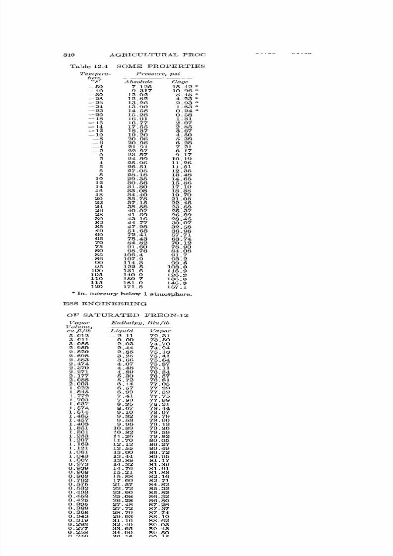
7/16/2019 Engenering Agriculture Perry
http://slidepdf.com/reader/full/engenering-agriculture-perry 325/422
310 AGRICULTURAl" PROCESS ENGINEERING
Table 12.4 SOME PROPERTIES OF SATURATED FREON-12
Tempera- Pressure, psi Yapor Enthalpy, Btu/lbIU1'e, Volume,OF Absolute Gage eu fl/l" Liquid Vapm'
-50 7.125 15.42 * 5.012 -2.11 72.31-40 9.317 W.n6 '" 3.911 0.00 73.50-30 12.02 5.45 .. 3.088 2.03 74.70-28 12.62 4.23 .. 2.950 2.44 74.94-2(i 13.26 2.93 .. 2.820 2.85 75.18-24 13.90 1.(i3 * 2.698 3.25 75.41-22 14.58 0.24 * 2.583 3.66 7.5.64-20 15.28 0.58 2.474 4.07 75.87-18 16.01 1.31 2.370 4.48 76.11-15 16.77 2.07 2.271 4.89 76.34-14 17.5.5 2.85 2.177 5.30 76.57-12 18.37 3.67 2.088 ,).72 76.81-10 19.20 4.50 2.003 6.14 77.05-8 20.08 5.38 1.922 6.57 77.29-6 20.98 6.28 1.84,5 6.99 77.52-4 21.91 7.21 1.772 7.41 77.75-2 22.S7 S.17 1.703 7.83 77.9S
0 23.87 9 .17 1.637 8.25 78.212 24.89 10. H) 1.57,1 8.67 78.444 25.96 11.26 1.514 9.10 78.675 26.51 11.81 1.485 9.32 78.796 27.05 12.35 1.457 9.53 78.90
8 28.18 13.48 10403 9.96 79.1310 29.35 14.65 1.351 10.39 79.3612 30.56 15.86 1.301 10.82 79.5914 31.SO 17.10 1.253 11.26 79.8216 33.08 18.38 1.207 11. 70 80.0518 34.40 19.70 1.163 12.12 80.2720 35.75 21.05 1.121 12.55 80.4922 37.15 22.45 1.081 13.00 80.7224 38.58 23.88 1.043 13.44 80.9525 40.07 25.37 1.007 13.88 81.1728 41.59 26.89 0.973 14.32 81.3930 43.16 28.46 0.939 14.76 81.6132 44.77 30.07 0.908 15.21
81.8335 47.28 32.58 0.863 15.88 82.1640 51.68 36.98 0.792 17.00 82.7160 72.41 57.71 0.575 21.57 84.82G5 78.43 63.74 0.532 22.72 85.3270 84.82 70.12 0.493 23.90 85.8275 91.60 76.90 0.458 25.08 86.3280 98.76 84.06 0.425 26.28 86.8085 106.4 91. 7 0.395 27.48 87.2881i 107.9 93.2 0.389 27.72 87.3790 114.3 99.6 0.368 28.70 87.74U5 122.8 108.0 0.343 29.93 88.19
100 131.6 116.9 0.319 31.Hi 88.62
105 140.9 126.2 0.293 32.40 89.03110 150.7 136.0 0.277 33.65 89.43115 161.0 145.3 0.258 34.90 89.80120 171.8 1.'57.1 0.240 36.16 £)0.15
* In. mercury below 1 atmosphere.
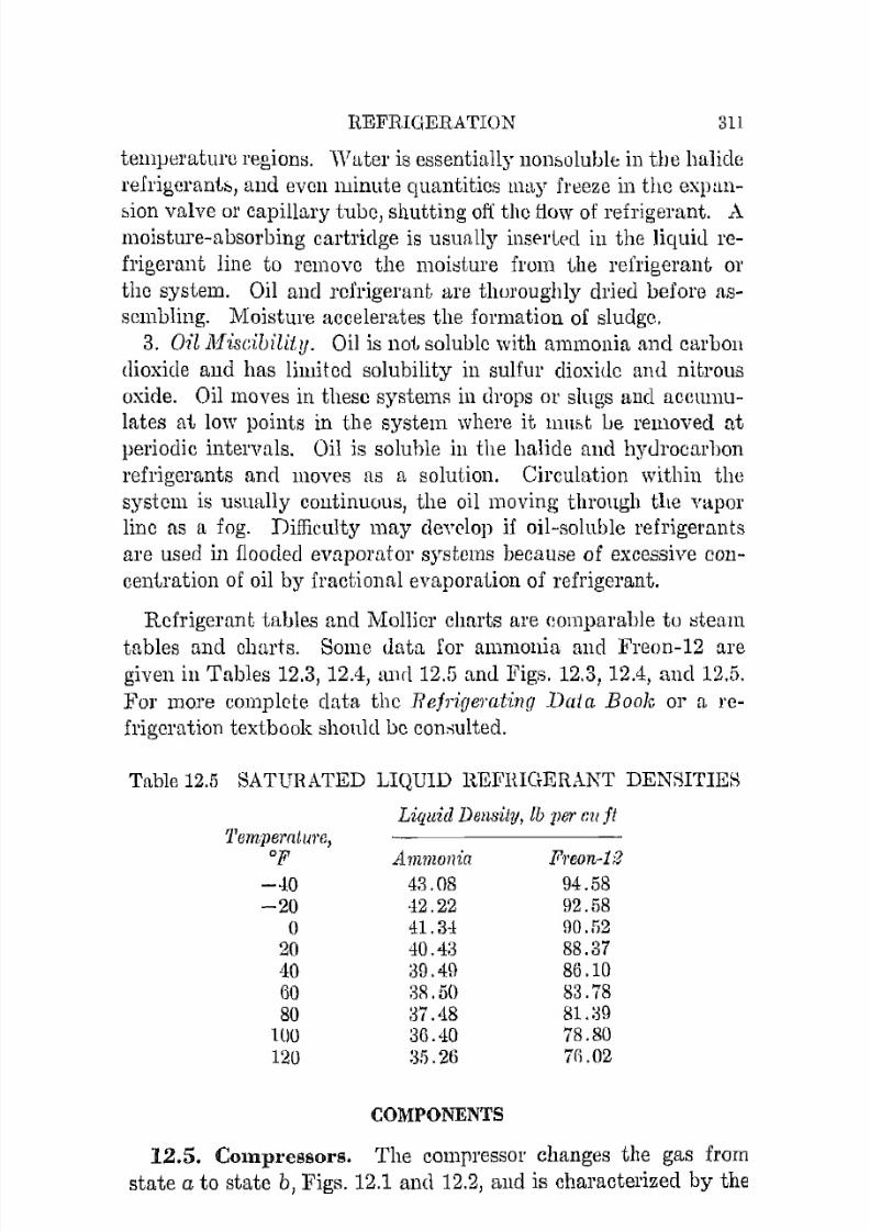
7/16/2019 Engenering Agriculture Perry
http://slidepdf.com/reader/full/engenering-agriculture-perry 326/422
REFRIGERATION 311
telll}leratUl'C regions. 'Vater is essentially non::,oluble in the halide
refrigerant::" and even minute quantities lllay freeze in the expan
bion valve or capillary tube, shutting off the flow of refrigerant. Amoisture-absorbing cartridge is usually inserted in the liquid re
frigerant line to remove the moisture from the refrigerant or
the system. Oil and refrigerant are thuroughly dried before as
sembling. Moisture accelerates the formation of sludge.
3. Oil MiscibiWy. Oil is not soluble with ammonia and carbon
dioxide and has limited solubility in sulfur dioxide and nitrous
oxide. Oil moves in these systems in drops or slugs and accumu
lates at low points in the system where it Il1Ilf>t Le removed at}leriodic intervals. Oil is soluble in the hnJide and hydrocarbon
refrigerants and moves as a solution. Circulation within the
system is mmally continuous, the oil moving through the vapor
line as a fog. Difficulty may develop if oil-soluble refrigemnts
are used in flooded evaporntor systcms because of excessive con
centration of oil by fractional evaporation of refrigerant.
Refrigemnt tables and MollieI' charts are (]omparable to ::;tealU
tables and churts. Some eluta for ammonia and Freon-12 aregiven in Tables 12.3, 12.4, amI 12.5 anel Figs. 12.3, 12.4, and 12.5.
For more complete data the RejT1:gemting Data Book or a re
frigeration textbook should be con:-;ulted.
Table 12.5 SATURATED LIQUID REFRIGERANT DENSITIER
Liquid Density, lb per ClI j t
'l'ernpemture,
OF-40-20
o20406080
100120
Ammonia43.08·12.2241.3-140.48:39.49:3R.50:37 .48:36.4035.2(j
COMPONENTS
Freon-if?94.5892.5890.5288.3786.1083.7881.a978.807().02
12.5. Compressors. The compressor changes the gas from
state a to state b, Figs. 12.1 and 12.2, and is characterized by the

7/16/2019 Engenering Agriculture Perry
http://slidepdf.com/reader/full/engenering-agriculture-perry 327/422
312 AGRICULTURAL 1'1WCESS ENGINEERING
volume rate uf the gas fit intake pressure and the pressure change
affected. Four types of compressors ltl'e in generl,l use.
1. Reciprocating or piston-type C0111pressors (Fig. 12.8) are
most extensively used. Small units directly connected to electricmotors are usee! for household refrigerating systems. Piston
diameters and strokes of less than an inch are common in the
latter systems. Multicylinc\er uuits are used for large industrial
systems. Reciprocating compressors are used for all refrigerantsand exclusively for those operating at high-pressure differentials,
for refrigemnts in the lower portioll of Table 12.2. The efficiencies (volumetric, thermal, and mechanical) m'e high.2. Rotary compreRS(JI'S (Fig. 4.4) are used with some success in
household and other small systems wherc prcssure differentialsare small or moderate. They are mechanically simpler than
reciprocating units, are quiet, have high volumetric capacity withhigh rotative speeds, ane! consequently occupy small space. Start
ing torque is less than for reciprocating compressors since there is
a smaller variation in pressure pel' rotative cycle. Tolerances
must be exceptionally close to insure volumetric performance.Lubrication is a problem since the vanes 01' other gas-confining
parts are usually spring or centrifugally loaded. Wear soon in
creases clearances, and the volumetric capacity decreases. The
mechanical efficiency may be low because of internal friction.
3. Gear compressors (Fig. 4.1) have the same performance fea
tures as rotary compressors except that the volumetric efficiency
may be less and the mechanical efficiency higher because of less
starting friction. Theil' chief usc is for boosting in compoundsystems.
4. C e n t 1 ' i f u g a ~ compressors (Chap. 5) are llsed extensively for
large systems using refrigerants with large specific vapor volume
and small pressure differential. Ail' conditioning systems usingrefrigerants from the upper portion of Table 12.2 might employ
centrifugal cornpressOl's. Single and multistaging is used, depend
ing upon the pressure differential. Performance is comparable to
a centrifugal air compressor. The volumetric capacity can beadjusted by throttling the discharge, a most convenient feature
not possible with positive disphcement units.
12.6. COlldensers. The condenser cools the compressed gas
to the saturation temperature and condenses it t.o a liquid, process

7/16/2019 Engenering Agriculture Perry
http://slidepdf.com/reader/full/engenering-agriculture-perry 328/422

7/16/2019 Engenering Agriculture Perry
http://slidepdf.com/reader/full/engenering-agriculture-perry 329/422
'NI 'as 83d '91 ' 3 ~ n S S 3 ~ d
"0 0 g 0 0 0 0 0
0m
'"1.0 \J)
0 ill 0N N '"'
III
0' "N N ...
0
N
0
I
_-I
0 0 " 0 0 00 ill 0 ill g g 0 ill 0 ill 0 W II)
M t>l N'"
0 CI) M N N '"'...
'NI 'oS M!i '!Ii ' 3Hnsmd

7/16/2019 Engenering Agriculture Perry
http://slidepdf.com/reader/full/engenering-agriculture-perry 330/422
HEAT CONTENT BTU PEll LB.
10

7/16/2019 Engenering Agriculture Perry
http://slidepdf.com/reader/full/engenering-agriculture-perry 331/422

7/16/2019 Engenering Agriculture Perry
http://slidepdf.com/reader/full/engenering-agriculture-perry 332/422
7/16/2019 Engenering Agriculture Perry
http://slidepdf.com/reader/full/engenering-agriculture-perry 333/422
REFRIGERATION 31:J
c'-d in Fig. 12.2. Some of the superheat, represented by Ii-c, lllay
be l'ernovcd by a special dc:<tlpcl'heatcr 10c!1ted between the COlll
pressor and the condenser. This can be a water-cooled heat ex
changer or simply a finned or extra-long bare pipe between the
compressor and condenser which permits heat to escape to the
room. The latent hent c--d is removed, and the liquid is sub
cooled to a point between e and d. Significant sub cooling cannot
take place llR long as the vapor is in conbet with the liquid. Suh
tooling, thrl1, results only if tho liquid iR in [L vapor-free heat
exchange regioll. Further subcooling, to c, takes plnce between
the receiver am! the evaporator.
FoUl' types of condensers are eOl1ll1lOn in agricultural work.
1. Al:j'-Cooled Condensers which make lIse of finned tubes are
usee! Oil systems lip to 3 hp. lJsual construction is vertical fin::;
with horizontal tubes, the vapor being fed in at the top, the liquid
flowing by gravity to the Imver part of the condcnser and thence
to the receiver. Air is forced through the condenser by a fan.
2. Shen etnd Tube Condensers consist of a cylindrical drum wiLha series of water tubes inside. Large-capacity units are vertieal,
smaller units horizontal. The horizontal unit usually serves as a
combination condenser and receiver. The water tubes arc located
in the upper portion of the cylinder so that the condensing surface
will not be covered with liquid.
I f the supply of water is ample and the cost low, the water is
used but once and then discarded. I f the supply is low or the cost
high, the water may be circulated through a eooling tower whereit is cooled by a portion evaporating. With a tower the actual
water usage may be only 2 per cent of that where it is w[lsted.
3. Combination A.ir- (tnd Water-Cooled Condensers are avail
[,ble for small systems that lllay be required to operate when ail'
temperatures are high, 95°}i' or higher. The water fiow is con
trolled by the high side-pressure so water is used only when high
temperatures of the air cause high head-pressure.
4. Evapom#ve Condensers are extensively used where water
supply (or disposal) or high temperatures are a problem. Water
is recirculated over the pipes of the condenser in a thin film, spray,
or shower. A forced draft of air over the wet pipes causes some
of the water to evaporate. The heat liberated by the condensing

7/16/2019 Engenering Agriculture Perry
http://slidepdf.com/reader/full/engenering-agriculture-perry 334/422
314 AGRICULTURAL PROCESR ENGINEERING
refrigerant, evaporates a small portion of the water passing over
the condenser tubes. The temperature at which the evaporation
takes place depends upon the nil' rate, kruperature, and humidity,
the water-to-air sU1"facc area and its heftt-and-vtlpOl' transfer co
efficient, the water-to-refrigerant surface area and its heat-trans
fer coefficient, and the temperature of the make-up water. The
water requirement for evaporative conrlensing is usually 2 to 5
per cent that required for sensiblc water condensing.
12.7, Evaporators. The nnit that does the cooling, that is,
extracts or removes the heat from the load is called the evaporator. The cooling proceSH is state change f-g', Fig. 12.2. The
pvaporator or hoiler as it is sometimes raIled is a heat exchanger,
and the principles of design and operation set ont in Chap. [)
apply.Evtlporator arrangement tl('pends upon Lhe C'xpectc(l duty.
Various armngenH'nts are shown in Fig. 12.G and are cliRcussed
under the letter indices.(a) A dry evaporator ('onsists of a single pipe or set of short
pipes wiLh headers (c). The liquid refrigerant is fed in at the top.(b) The wet evaporator is comparable to the dry evaporator
except the liquid is introducecl at the bottom and flow il:! upward.
Upward refrigerant movement gives somewhat better heat trans
fer than clownward movement because of more vigorous mixing ofthe liquid and vapor. The dry evaporator facilitates oil move
ment. Oil flows through the unit by gravity; thus both oil solublefl,nd nonsoluble refrigerants can he used. Oil must be continu
ously removed from the wet evaporators as a refrigerant-vaporoil fog for both soluble and nonsoluhle refrigerants 01' be chained
off at periodic intervals in the c r t ~ e of nonsoluble refrigerants.
Oil removal by fog is satiidaetory for tIll' soluble refrigerants
unless the refrigerating rate is low in which case the fog action
lllUY be insufficient to carry out the oil. Fog oil removal from
nonsoluble refrigemuts may not be entirely satisfactory even at
high refrigerant rates since the oil moves as drops or slugs, not as
a solution.(c) A heade1· or manifold system is superior to the single-pipe
system. Spent vapor is removed quicker, and better h e a t - t r a n s ~fer coefficients result. The pressul'e drop thl'ough the unit is less
because of a shorter vap0l'-travel path. A single-pipe evaporator

7/16/2019 Engenering Agriculture Perry
http://slidepdf.com/reader/full/engenering-agriculture-perry 335/422
REFRIGERATION 315
is used only for small installations where cost and fabl'iclItingconvenience lIrc more important thlln performance.
(d) A flooded evaporator is one designed for maximum heat
transfer effectiveness by 'Ifioocling" the inside of the heat-tl'ansfel'
a. Dry evaporator
c. Header orlnanifoldsystem
e. Shell and tubeevaporator
b. Wet evaporator
d. Flooded evaporator with
an accumulator :
ul.,.
~ ! [ I~ ~ : ;
~ . ~ ~
j ----- t=II III IIIII III II Ij I I I I I I I ~ -
,0
g. Heat exchangeror regeneratorIce bank evaporator
Fig. 12.6. Various t.ypes of evaporat.ors and accessories.
surfaces with liquid refrigenmt. The surfaces arc flooded bymaintaining the liquid refrigerant level in the evapomtol' ab()ve
the transfer surfaces by a float (d, e) or other level-maintaining
device. ,Vet evaporators are frequently called flooded evaporators. A distinction should be made between them on the basisof performance and design.
An acc1{:mulato1' is used with the flooded system to improve
performance further. The coil-and-header system are designed
for vigorous liquid boiling action which facilitates heat transfer.

7/16/2019 Engenering Agriculture Perry
http://slidepdf.com/reader/full/engenering-agriculture-perry 336/422
316 AGRICULTURAL PROCESS ENGINEERING
Forced circulation of Lhe liquid by a pump may be employetl to
provide even better performance. Because of the vigorous acLion,drops of refrigerant are carried toward the vapor disch:.trge port.These drops are separated from the spent vapor and collect inthe "accumulator." The liquid-frce gas then returns to the compressor. This Elystelll it:> not completely satisfactory for oil-soluble
refrigerants. The gas dif;clwrge action it:> not vigorom, enough tocarry out the oil Lhat accmnubtes in the unit in solution. Non
soluble refrigerants permit the oil to R('ttle out, and it is drainerl
offaL
periodic intervals.(e) A shell and tube evaporator has Lite same operational cha1'aeteribti('s as the accumulator sysLem. I t is used for cooling brine,water, or other liquids. Tlte cooling maLerial ll1URt not be per
mitted to freeze.(f) The ice-bank evn,porator is used where large quantities of
"chilled" ,vater at 32 D F are neerled. Evaporation takes place ina series of pbtCH or bank of tubes which are immersed in a tank
of water. During periods of low-water demand ice accumulates
on the plates. The icc is then available for cooling the waterduring peak-demand periods. This procedurc perll1itR a smallercompreSflor to be used than would be required with the non-ice
system.(g) Evaporator performance cttn be improved by installing a
heat exchanger or regenerato7· immediately following the evapo
rator. Thus, Fig. 12.2, state a is moved toward a' and e toward
e' , f in turn moving toward 1'. This decreases the pcrcentage of
flash vapor at the expansion valve but increases the superheat at
the compressor. Subcooling to e can be produced by locating the
heat exchanger so its trailing end is in the liquid evaporating
region.
12.8. Expansion Valves. The expansion valve is uscd to
regUlate the rate of flow of liquid refrigcrant into the evaporator
at the evaporating rate. Four types of valves are used.
1. ManllaUy Adjusted N eelile Valves may be used in large t:>ystems where loads are relatiYely constant and an atLendant is on
duty. Their advantageous features 111'C quick adjustment, sim
plicity, and low first cost.
2. Flo!Lt )Talves are actually automatically adjusted needle
valves since they are so pOflitioned that the incoming liquid rat.e

7/16/2019 Engenering Agriculture Perry
http://slidepdf.com/reader/full/engenering-agriculture-perry 337/422
REFIHGEHATION 317
equals the evaporating; rate. They are med, [is prcyiously dis
cllssed, in flooded f'y:-;tcllls with accumulators.3. CalJil1ary 'rubes lIrc used extensively in household refrigera
tion and other slllall systems. They are suitable only for systemscomposed of a single compressor and a single evaporator. Theliquid passes from the high to the low side through :1 small tubeof such a diameter and length that the rate of flow at operu.tillgpressure does not exceed the evallomting eapacity at the designload. The system is simple since there are no vah·es, except inthe compressor, and [\ receiver is not used. TIle system clements
t " H ~ ~Fig. 12.7. Principles of iJll' tJ'errnal e X j l a l l ~ i ( ] n y a l \ ' ( ~ .
are located relative to cneh other so tlHLt when operation haseeased, the liql1icl will flow into the evaporator and/or condenserand pressures will equalize throughout. the system. Consequently,
there is no pressure differential across the compressor when it
starts. This permits a low-starting torque motor to be usecl. The
quantity of refrigerant charged into the system must be controlledcarefully.
4. Thermal EX1)(tnsion Valve, Fig. 12.7, operates on the basis
of the number of degrees of superheat in the spent vapor leaving
the evaporator. Thermal expansion valves are used on evapo
rators (a), (b), and (c), and 011 systems of a wide range of sizes
and those with more than one evaporator. They arc especially
applicable for field-assembled systems with automatic control
and variable-cooling load.The thermal sensing bulb is usually filled with the same fluid
used for the refrigerant. Consequently, the downward pressure
on the diaphragm due to a temperature of the bulb is comparable
to the upward pressure on the diaphragm due to the saturated
7/16/2019 Engenering Agriculture Perry
http://slidepdf.com/reader/full/engenering-agriculture-perry 338/422
318 AGRICULTURAL PIWCESS ENGINEERING
pressure of the refrigerant within the evaporator. This force rc
ferred to the spring reaction maintains a proper opening of the
valve for all temperatul'es and loads, the design or ac1justed
superheat applying at all times. Consideration of these data and
the physical characteristics of i,lw valve will show that:
1. The superheat to the senRing bulb is eOlmLant at all loads.
The temperature difference botween the boiling liquid and the
material being eoolo(l111ay be greater than the superheat but never
less.
2. The liquid rate is conLrolled on the basi:-; of the heat load.Thus, the amount of evaporator surface used for heat exchange is
controlled by the heat load.
3. Liquid flow is sLopped when the compl'etlsor stops. Thisfeature facilitates control which is discussed later in this chaptcr.
SYSTEM DESIGN AND BALANCE
The heaL and mass balance for a system can be expressed bytho following equation.
12.9. The Evaporator:
W",c(h - i2) = AU(h - i3) = TV,. (h g l - hf ) = q (12.5)
where W", = mass rate of medium to be cooled, Ib per hr.e := specific heat of medium.
t l - t2 = temperature drop of cooling medium.
Wr = refrigerant rate, lb per hr.hgl = heat content of vapor leaving evaporator, Btu per lb.
hi = heat content of the liquid refrigerant entering theevaporator, Btu per lb.
A = eVtlporator heat-exchange area, sq It.b = temperature of the evaporating refrigerant., OF.
q = heat rate, Btu pel' hr.U = heat-transfer coefficient, Btu per ChI' sq ft OF be
tween medium entering exchanger and refrigerant).The refrigeration load is defined by (1) the heat rate q, (2)
original and final temperature hand t 2 , and perhaps (3) relativehumidity. Commercial evaporators are rated on a heat rate per
degree temperattu'e difference, T.D., h - t3 in equation 12.5.

7/16/2019 Engenering Agriculture Perry
http://slidepdf.com/reader/full/engenering-agriculture-perry 339/422
REFRIGEHATION 319
The iituclent dlOuldllllcierstand that a rigorous treat.ment at' the
heat-cxehallger performanee \vuuld l'elluil'c that the log-mean tem
perature difference be used. Such a diffcrenee would bc used inanalyzing a unit that was not test rated on the basis of tl and t3'
This rating procedure is used because of cOl1veuicnce. Cooling
loads which can be carried with a large T.D. e::m be handled with
an evaporator of small effective area A. Note however that a low
evaporator temperature 'will require a low side-pressure and a
compressor of greater volumetric capacity will he needed. The
T.D. is usually limited by the p o ~ s i b i l i t y of freezing, frost forma
tion, or dehumidification of the air.12.10. Defrosting of evaporators for ail' cooling above 34°F
is brought about by using an evaporator of sufficient size so that
the load can be handled with only part-time operation. Frost
accumulating during the running eycle is meltell during the off
cyele. This procedure, in addition to defrosting, helps to main
tain humidity if high humidities are deiiil'ed.
Evaporators for below freezing temperatures nrc designed with
fins a greater distance apart or with bare coils so that moderatefrost or ice accumulation will not affect ail' flow. Defrosting is
by hot water, electric heaters, 01' hot gas. Hot gas from the high
side of the system is piped to the evaporator by a series of con
necting lines [mel valves. Operation may he ll1anual or automatic.
:Frosting may be prcventecl by continuous circulation of a brine
ovcr the evaporating surface. The brine picks up moisture frOtH
the surface and must be reeoncentrateel or replaced at intervals.
12.11. The Comllressor:
WrVg = (iOEvDN rpm (12.6)
where Vg = specific volume of the vapor entering the compressor,
at low side Pl'CS!:lUJ'C, eu it per lb.
Ev = compressor volumetric efficiency, GO to 75 per cent for
small reciprocating compressors.
D = piston displacement, cubic feet per piston revolution.
N = number of pistons.
rpm = compressor speed.
Horsepower per ton of refrigeration (thermal)200 (hb - ha)100
hgl - he X Ec(33,OOOj778)(12.7)

7/16/2019 Engenering Agriculture Perry
http://slidepdf.com/reader/full/engenering-agriculture-perry 340/422
320 AQRICUI,TURAL PROCESS ENGINEERING
where hg, = heat content of vapor leu,ving evaporator, Btu pel' lb.
he = heat content of liquid entering evaporator, Btu per lb .hb = heat content of vapor leaving cornpreSSOl', Btu pel' lb.
h", = heat content of vapor entering compressor, Btu pel' lb.
Ec = compression efficiency, 65 to 80 per cent (estimated). .
EquaLion 12.6 define::; the capacity of a compressor in terms of
its speed, its physical characteristics, and the mass rate of the
Fig. 12.8, Conventional c o m j J l ' e ~ ~ o l ' - C o n c J e l l S O l ' unit. (Collrtesy the Cope-land Co.)
refrigerant. The vapor volume mte represented by the product
Wrvu must be the same as that for the conditions jn equation
12.5 with corrections for line friction. The compressor capacity
must be balanced with the capacity of the evaporator. A com
pressor with more capacity than that specified for the desired
conditions will move a greater volume 01 vapor at a greater
specific volume. This will lower the suction pressure and evapo
rating temperature and increase the mass evaporation rate. The
*The compression efficiency is defined as the ratio of the work requiredfor an isentropic compression process to thCl actual work required. Fewdata. are available.

7/16/2019 Engenering Agriculture Perry
http://slidepdf.com/reader/full/engenering-agriculture-perry 341/422
REFRIGElL\TION 321
fldclitional capacity will manifest itself by lowering the e v a p o ~rating temperature ta in equation] 2.:3 with increased capacity of
the evaporator und appropriate adj1lstments of the other factors.
12.12. A Condensing Uuit consists of a cmnpressor and motor
and either an air-cooled fmnml condenser or Rhell and tuhe water
cooled condenser (Fig. 12.81. Rating in Btu per hI' at various
('vHporntor temperatures and ambient air temperature or con
densing wakr temper::d,ures is given. Since most compres:,:ors are
belt driven, ('apneity can be further adjui:ited by change of e o m ~pressor speed.
Equations 12.G and 12. 7 are useful for estimating po\\' ' ' requirell1entR for conditions not eoYcl'ed by comml'reial data.
CONTROLS
Refrigeration control may be considered from the standpoint
of (1) individual component control, (2) safcty of both equipment
and operator, and (3) temperature and perhaps humidity control
of the medium being cooled. Temperature and humidity will beconsidered.
12.13. Motor Circuit Thermostats are llsed on single-evapo
rator systems with capillary tube, thermal expansion valve, and
float-controlled evaporators. Temperaturc control is as accurate
as the thermostat. Expansion or float valves that do not com
pletely restrict liquid flow during the off-cycle may cause com
pressor flooding. Compressor damage or motor overload may
result when the unit starts.12.14. A I ..ow·Side·Pressure Switch opens and closes the
motor circuit on the basis of the low Ride-pressure which is
directly related to the temperature of the evaporating liquid as
shown in equation 12.5. As cooling takes place, ta and the cor
responding refrigerant saturution pressure drops. The decreased
pressure opens the switch. The residual liquid refrigerant soon
assumes ambient temperature, the p r c s s u r ~ rising to the corre
sponding saturation pressure. A rise in amhient temperature
causes a pressure rise that closes the circuit. Expansion and com
pressor valve leakage are compensated for by automatic com
pressor operation. Frost accumulations decrease the U valve
of the evaporator, and the controlled temperature rises. The
controlled temperature rises as the refrigerating rate increases

7/16/2019 Engenering Agriculture Perry
http://slidepdf.com/reader/full/engenering-agriculture-perry 342/422
322 AGRICULTUHAL PROCLSIS ENGINEERING
because the evapOlatmg-Iefllgelctnt ane] coolmg,-matellal tem
pewtme dlffClence l l l C l e a : ; c ~ TIll'3 method of contlOll'> '3atl&factory only 101 'llllgle-evd,pOlatOl '>y'>tems un1e<;s acichLlOnal contlo]
features ~ u c h as those chscu,>scd below a l e added to the system
12.15. Magnetic Valves opel,ltcll by a thermostat ale f10-
quently used for contlol I II multIple-cvapOlatOl systems, FIg,
L , ,.
110 volts =J - - - -- j i l - - - - - - - - - - - rl=':- l1
' I 81
S1 1 11 1 1, ::PM " 8,
! \--iiI-J
V ' il, i l l...__
J -" "J hermostat J hermostat
34· 50' 10'
,
FIg, l2\) Mult11J!e-eV:ljJOJ :ltOI ~ y s t e m opa,ttmg flam 'L bmgle romp! essOlThe C O l l l P l C ~ ' ( ) l motol I'> opellltod hy a ImV-"lde-pI8&Sm8 sWltch activated
by the low s)(lc PICb5UlC of the lowe5t LlInpelatUlf' load, loaF I II thIs ('''
dmple The solC'nOlri'l 01 th e Inghel-lempClatme 10 ,d s 'ue contlolled by
th81mosiats L!CjUldlefug81dllt IS let mto the c\,tpOIato! only when tool
mg IS lequned The evapOIatlVe ] J I C ' s ~ 1 1 I e - m , l l n t , L l l l l l l g valve PM holds
the ple'l'lure m tlw e\a.l'Gl'ltol of the 34'F load ahove the p \ ( ' ~ " m e 1Il. thl'
vapOl letUln lllle TillS pC'lmlis humIdIty LOnilOl 01 mmunum evapowtOl
flOsLmg by cOlltrolhng the evapolatmg t( lllpeJ::ttUlE' The eV:lporatmg tC'lJI
per,\cure of ihe 50'F load 1" tl1[' '>amp 1.8 thai of tll(' lO'F load A vapOl
(iIsc,halge ~ o l e n O l d can be u9NI l l l ~ L l 1 1 e d all the 50'F load to proVldrmale accmat(' tcmpf'latme ('onllol TIm valve confines the l C ~ l ( l l i a l hqmd
If'fllgelanc III the evapOlatOl, thu'l ~ t o p p l n g the rcf1'lgf'1 rttmg acilon at the
p).act plescubcd tempmatUl p WIthout t im , alve the l ' e ~ l d u 11 lIqUId would
evupOlate and the tcmpe1,ttUlc might dlOP below Lhe contIolled tempel'l-
tUle Thl'3 valve 19 men only whtrp hIghly C,{,lLt contJOl!s leqUlred
12 9 The thentlo'Stat opens t Ite valve permIttmg lIqUId to entel
the evaporator The suctlOU PIC%UlC s'Altch IE, set for a pre'lsmc
somewhat below the opel'atmg pI essure of the evaI'm ator MagnetIc valves a1 e also used m combmatIOn with manual and float
expansIOn valves to facIlltate ope1atlOll
12.16, Evaporative.Pressure.Maintaining Valves, also called
back-plcssure control valves, ran be used 011 m u l t J p l e ~ e v a p o r a t o rsystems to control the evaporatl11g plebsure in any evaporator

7/16/2019 Engenering Agriculture Perry
http://slidepdf.com/reader/full/engenering-agriculture-perry 343/422
REFIUGERATlON 323
Without them, the evapomtillg prcssure llnd temperature of all
the evaporators in a multiple system arc those of the lowest prcs
sure unit with slight variations for line friction. I f i t z e l ' o - d e g r e [ ~room and n :3-1-clegree room arc to operate on the ~ m n e compressor
it will probably be advisahle to operate the higher temperature
j 'oOlll with a higher pressure evaporator in order to minimize coi1
f)'(Jsting and, if desired, to maintain [ I high relative humidity in
the room. This i:;; done by using a pressure-Illaintaining \ , ~ l l v es1101\'11 in principle ill };'ig. 12.10 and IDeated in }i'ig. 12.9.
Fig. 12.10. Schenmtie sketch of Ull evaporative Pl'0Bf3Ul'c-maintaiuing ynlve.
The thermodynamic):; of the process nre shown in Fig. 12.] 1.
The flow through the valve is irreversible adiabntic j state ehange
- a', The power state path for the higher pressure unit would
be ((2 - b2 if separate compreSSDrs were used for each load, the
power energy for the systenl being
(12.8)
W 2 and H\ are the respective refrigerant weight rates. The total
power for the l:iystem designed for a pressllre-maintaining valve
and a Bingle compressor is
(12.9)
The difference between equations 12,8 and 12.9 is the extra po\verrequired owing to the pressure-maintaining valve.
lhlltiple-evnporator systems with an operating tempel'ftture
range and pressure-maintaining vnlves 011 the high-temperature
evaporators are economically sound if the major portion of the

7/16/2019 Engenering Agriculture Perry
http://slidepdf.com/reader/full/engenering-agriculture-perry 344/422
324 AGRICULTURAL PROCESS ENGINEERING
/,.t
/I
p l ~ - - ' ~ - - - - - - - - - - - - - - - - - - - - ~ ~ la '
h
/ '.
/ ,. ,.I ,.
1/ 1/",. ,.I /, /
I I,. /
I /I I
Fig. 12.11. Tho t1wnnouyullmic Pl'OCf'HS of the evapol'lItive ] l l ' ( ' s ~ \ l r e maintaining valve and its relution to tJIC onth e system.
load is a low-temperature load. I f the major portion of the land
is high temperature, independent, systems may be advisahlr.
HEAT PUMP
The heat pump is a refrigeration machine installed where the
heat discharged from the condenser is desired rather than the heat
absorbed by the evaporator. The heat pump may be regardedas a device that lifts or "pumps" heat energy from a low-tem
perature source for use at a higher temperature. It is used satis
factorily for space heating by lifting heat from the ground, outside
air, or bodies of water at a lower temperature than the space to
be heated. Other uses, existing and proposed, lila,ke use of both
evaporator and condenser energies.Heat pumps may be fitted to a variety of operations, e.g.,
1. Comfort heating and cooling of buildings.2. Water and other liquid heating, domestic and industrial.
3. Evaporating, concentrating, :lllrl distilling.
4. Drying.
5. Simultaneous heating and cooling, e.g.,

7/16/2019 Engenering Agriculture Perry
http://slidepdf.com/reader/full/engenering-agriculture-perry 345/422
REFRlGEHATION 32;j
a. \Va tel' cooling and spacc heating.
b. Heating and dehumidifying, domestic and industrial.
c. \Yater heating and space couling.
12.17. Coefficient of Performance. The c [ ) e l f i ( ~ i e n t of per
fonnance of a heat pump refers high-temperature condenserenergy to the driving energy so that the cycle c.o.p. is (referringto Fig. 12.2)
(II", - hd)/(hb - h,,) (12.10)the Carnot c.o.p. is
TIl / (TIl - Tc) (12.11)
Since the c.o.p. relates the useful heat output as refrigeration in arefrigerator or heat energy input in a heat pump, the c.o.p. for
simultaneous usage snch as 5CL could be considered as
(12.12)
The smaller the difference in temperature betwecn the eV[tporntorand condenser, the greater the e,o.p. and the grenter will be the
output per unit of mcclumical input.
A decision to install a heat pump in lieu of a conventional gas,oil, or other heat energy source should be made on the basis of
an economic and convenience study. Factors that must be con
sidered are initial cost, length of life, npkeep, operating cost andcontinuity of power source, operating attention, ete. For example,a gas-fired hot-water heater might be 70 pel' cent efficient ther
mally; thus, 14:00 Btu must be supplied for each 1000 Btu tn,ken
up by the water. A heat pump with a c.o.p. of 3.5 would needonly mechanical energy the equivalent of 290 Btu.
SOURCES AND SINKS
The "source" of heat for a heat pump can be a steady-state
source such as air or water. The mass rate would be controlled
so that the difference in temperature between the evaporating
refrigerant and the cooling medium is nearly constant for variousheat rates. Air, wel1 w a t ~ r , stream water, liquid manufacturing
wastes, etc., can be used.Systems installed in areas where air and water temperatures
are low or where a sufficient supply of water or other heat-source
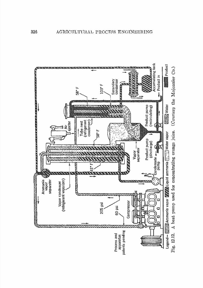
7/16/2019 Engenering Agriculture Perry
http://slidepdf.com/reader/full/engenering-agriculture-perry 346/422
326 AGRICULTURAL PROCESS ENGINEERING
u ,....'"CJ ci0 u0:
I...(J.)
·aLL. >1
LL. 0·0:g
(J.)~"""'"-.:;;:l<:>
Q.._.,
5 a.i
'".:g,!
~2 (J.)
ro$: §
~ H0
. bl l
ro .S·c ~E tl
(J.)ro
'"CJ s:!·s 00" '":;
f:)~ '- H
""0
t&l
0;:J
'"a. P-o
Co
"" §n ro0 ·c<'J 0
P-
E ~E (J.)-0: ,.<:1
~ -«iOIl
"grn:6 + t<ictJ-E c "CJ >-'!
~ ~ t : C'I
'",....,
~ ~ 2 ~ biJCo t : .. J~ " ' Q )~.. 1Oa.
7/16/2019 Engenering Agriculture Perry
http://slidepdf.com/reader/full/engenering-agriculture-perry 347/422
REFRIGERATION 327
medium is unavailable lnay require a trallsient source. A tran
sient source is a pond, well, or series of wells, the earth, or other
stationary heat source with sufficient capacity and transfer prop
erties to supply the heat at a satisfactory rate. Poor 11er1'ormanoo
may occur if, when designing the source, deGrease in heat transfer
due to shallow thermal gradients as operation continues is not
recognized.
A "sink" is a heat disposal for condenser heat. The t-Iame char
aeteristics apply as for the somce.
A heat pump used for concentrating orange juice is an exmnplc
of an agricultural heat-pump installntion. Fig. 12.12 shows aschematic a1'l'angement of the system and the operating condi
tions. The unique feature is the use of the refrigeration evapo
rator for condensing the vapor removed frolll the orange juice.
The compressor is an 11 by 10 in. 4-cylinder 300-rpm unit with
[ i volumetric efficiency of 91 per cent. The orange juice is con
centrated from 11 to 55 degrees Brix (specific g1'ayity of 1.03 to
l.16) .
Note that the power required is nearly an i11\'e1's8 function ofthe heat-exchange area. I f the heat-exchange areas were in
creased the compressor power could be reduced. The optimuJll
Hize of these factors must be hased upon a cost analysis.
REFERENCES
1. Macintire, H. J., and Hutchinson, F. W. Refrigeration Engineering.
Second Edition. Wiley. 1950.
2. Myers, W. P., Jr. Refrigeration Controls. Refrig. Eng. 57:884ff. Sept.,1949.
3. Penrod, Estel B. Development of the Heat Pump. Ky. ElLa- Expt.
Stn. Bull. 1, 4. 1947.4. R.abel', B. F., and Hutchinson, F. W. Re/1"igemlion and Ail' Condition
ina Engineering. Wiley. 1945.
5. 'l'he Refrigemting Data Book. Basic Volume. Sixth Edition. TheAmerican Society of R.efrigerating Engineers. 1949.
6, The Refrigerating Data Book. Refrigeration Applications Volmne.
Third Edition. The American Society of Refrigeration Engineers.1951.
PROBLEMS
1. Ammonia is required for a 3-ton refrigeration system with an evaporating temperature of -loaF. The condenser will be water-cooled and

7/16/2019 Engenering Agriculture Perry
http://slidepdf.com/reader/full/engenering-agriculture-perry 348/422
328 AGRICULTURAL PROCESS ENGINEERING
will opemte on a 10°F dillerential. Tap water temperature is 70°F.Determine the following. Assume saturated conditions.
a. High find low side-pressures (gage).b. Compressor displacement rate; assume volumetric efficiency 85 pel'
cent.c. Thermal horsepower required, assume thermal efficiency 90 PCI' cent.d. The liquid ammonia mte in ]Jinls per minute.
e. The capacity in tons if the evapomting temperature is raised to I5·F.
The compressor capacity is unchanged.
2. Work problem 1 with Freon-12 as the refrigerant. Compare compressordisplacement and liquid rate. Which refrigerant would you recommend
for a large installation? Why?
3. A I-ton. Freon-12 system has ( l l l evaporator temperature of 32°F and ahigh side-pressure of 90 psig. Liquid refrigerant enters the evaporatorat GO°F. Vapor enters the compressor at 50°1<'. Use the MollieI' chartand determine:
a. Per cent flashing into vapor as the liquid passes through the expalmionvalve. Calculate from enthl11py values.
h. The coefficient of performance.c. The thermal horsepower.
d. The thermal horsepower if the vapor enters the compressor with nosuperheat.
c. The compressor cli:;placement, assume 80 per cent efficient.
4. An evaporator pressure-maintaining valve holds a 30 psig C'vaporatinp;pressure against a 5 psig low side-pressure. The vapor enters the valvpsaturated. Determine the energy in it Ib 1)el' lb of refrigerant expendedin the process.
5. Show by a MollieI' chart the necessity for the secondary condenser ofFig. 12.12.
o. Determine the coefficient of performance of the heat pump of Fig. 12.12.
7/16/2019 Engenering Agriculture Perry
http://slidepdf.com/reader/full/engenering-agriculture-perry 349/422
CHAPTER 13
PI'oress Condition OhseI'v lltions,
Records, amI CoutI'Ols
NOMENCLATURE
11 = surface area of sensing element, sq ft.C = heat cnpaeity of sensing clement, Btu per of .
Eg = voltage genel'l1ted by tlwrmocouple.E", = voltage at instrument.
h = unit surface thermal eOlldu(:tancc, Btu per (OF n,2 hr).
I = eurrent, amp.
Ire = resistance of external circuit, ohms.
Rm = resistance of instrument, ohms.t = temporature of sensing clement, "F.
ta = temperature of adjacent medium, "F.tHv = average air temperature, of.tp = amplitude, of .
a = lag of sensing element in periodic environment, radians.
o = time, hr.
Op = period of wave, hr.
The operating conditions of a process frequently must be con
trolled within specific finite limits. Cold storage and freezing,pasteurization, homogenization, washing, drying, and dehydration
are processes that require temperature, pressure, flow rates, etc.,to bc controlled. Temperature is the most frequently controlledcondition. Although this chapter deals with temperature in the
main, adequate treatment of some other factors is included.
OBSERVATIONS, TEMPERATURE
13.1. Liqui<l.in-Glass Thermometers. Liquid-in-glass thermometers are suitable for observing teluperatures up to a p ~proximately 950°F. Mercury is used as the actuating fluid fortemperatures between _35 0 and 950°F. Mercury cannot be used
329

7/16/2019 Engenering Agriculture Perry
http://slidepdf.com/reader/full/engenering-agriculture-perry 350/422
330 AGRICULTURAL PROCESS ENGINEERING
<l)
:S
'S
~r - - - - - - - - - - - - - - - - - - - - - - - - - - - - - - - - - - - - - - - ~ ~

7/16/2019 Engenering Agriculture Perry
http://slidepdf.com/reader/full/engenering-agriculture-perry 351/422
PROCESS CONDITIONS 331
for temperatures below its freezing point of -38°F. Alcohol or
other organic fluids are used for atmospheric temperatures nncI for
temperatures down to -200°F.The accuracy is usually 1 per cent of the range when properly
installed and operated. Individually calibrated thermometers
with a high degree of accuracy can he securell. The amount of
immersion and conditions surrounding the exposed portion of
the thermometer affect accuracy. The amount of immersion is
usually specified by the manufacturer. ·Widely fiuctuating am
bient temperatures in the exposed portion may cause observa
tional errors due to expansion and contraction of the glass tube.Glass thermometers are available in a number of formRi some
are shown in Fig. 13.1.
13.2. Bimetallic Thermometers. Bimetallic thermometers
can be made comparable to mercury glass thermomct,ers in ae
curney, temperature range, and uses.
Two strips of dissimilar metal, one generally being Illvar which
has a very low coefficient of thermal expansion, are welded or
fused together as shown in Fig. 13.2. Changes in temperaturecause movement of the free eml which can be linked to an indi
eating needle. The bimetal strip can be straight or coiled, Fig.
13.2.
This type of thermometer is superior to the glass thermometer
in that the bimetallic thermometcr is 1110re rugged, easier to read,
and is not affected adversely by amhient temperatures. The
bimetallic unit must be immersed eompietely. Since the relative
motion is essentially linear with tempcrature, calibration is easyand simple motion-transfer links can be used.
13.3. Pressllre Thermometers. A pressure t.hermometer
consists of a sensing bulb and a Bourdon tubc, bellows, 01' a
pressure spring connected by a capillary tube. A temperature
change at the bulb caUses a change in pressure within the system.
The resulting movement of the pointer linked to the pressure
spring indicates the temperature at the bulb. Three types of
systems are used.1. M erc1b1'y-Filled Systems. Steel or stainless-steel systems are
completely filled under high pressure with mercury, which has a
much greater coefficient of thermal expansion than the steel. C o n ~sequently, a change of temperature will cause a relative volume
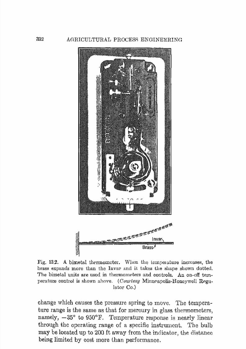
7/16/2019 Engenering Agriculture Perry
http://slidepdf.com/reader/full/engenering-agriculture-perry 352/422
332 AGRICULTURAL PROCESfi ENGINEERING
Brass
Fig. 13.2. A bimetal thrrmomcter. When the lCIlljlCll1ture increases, the
brass expands more than the Invar and it, takes the shape shown dotted.
The bimetal units are used in thernlonwters and controls. An on-off tem
perature control is shown above. ( C 0 1 ~ l ' t e . s y Minneapolis-Honeywell Regu-lator Co.)
change which causes the pressure spring to move. The temperature range is the same as that for mercury in glass thermometers,namely, -35 0 to 950°F. Temperature response is nearly lineal'through the operating range of a specific instrument. The bulb
may be located up to 200 ft away from the indicator, the distancebeing limited by cost more than performance.
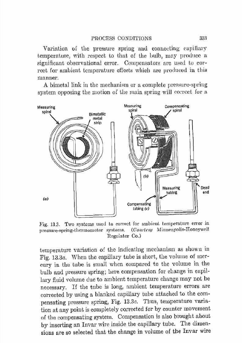
7/16/2019 Engenering Agriculture Perry
http://slidepdf.com/reader/full/engenering-agriculture-perry 353/422
PROCESS CONDITIONS 33S
Variation of the pressure spring alld conneetlng cupillnq
temperature, with respect to that of the bulb, Il1tly produce a
significant observational error. Compensators are used to correct for ambient temperature effects which are produced in this
manner.A bimetal link in the mechanism or a complete pressure-spring
system opposing the motion of the main spring will correct for fl,
Measuringspiral
(a)
Measuring
Compensatingtubing (c)
Compensatingspiral
Deadend
Fig. 13.3. Two systems used to correct fot' ambient temperature error in
pl'essure-Rpring-thermomctel' systems. (C'o Ill'tcsy Minneapolis-Honeywell
Regulator Co.)
temperature variation of the indicating mechanism as shown inFig. 13.3a. When the capillary tube is short, the volume of mercury in the tube is small when compared to the volume in the
bulb and pressure spring; here compensation for c h ~ n g e in capil
lary fluid volume due to ambient temperature change may not he
necessary. I f the tube is long, ambient temperature errors are
corrected by using a blanked capillary tube attached to the com
pensating pressure spring, Fig. 13.3a. Thus, temperature variation at any point is completely corrected for by counter movement
of the compensating system. Compensation is also brought about
by inserting an Inval' wire inside the capillary tube. The dimen
sions are so selected that the change in volume of the Invar wire

7/16/2019 Engenering Agriculture Perry
http://slidepdf.com/reader/full/engenering-agriculture-perry 354/422
334 AGRICULTURAL PROCESS ENGINEERING
due to a ehange in temperature equals the change in capillary
mercury volume.
A change in elevt1t.ion of the bulb relative to the pressure springwill cause a shift in the preSSUl'e reading equal to the cleva Lion
head. A simple a d j u s ~ l l 1 e n t is provided to readjust the instrument
after installation in a particular location.Oil and other liquids arc also used in liquid-filled instrumentR.
---~ ~Liquid- - - -- - - ----- ------------- - - -
(a)
/ L iqU id
Vapor
.==:-...::...:.-=.
- - -=-- ~ --Liquid
-----
-- -==----=
(b) (c )
Liquid
Inert-liquid
Fig. 13.4. Types of fill foJ' vapor-pressure temperature-indicating SysLl'IllS.
The inert liquid must, not react wit.h the vaporizing liquid 01 ' pl'ollueo U
significant vapor pressure l1 t the operating tempemtul'cs.
2. Gas-Filled Systems. Systems filled with high-pressure g n ~ ,usualLy nitrogen, perform according to the gas law so that thesystem volume and l'el:lUltant mechanism movement arc nearlyproportional to the change in temperature. Compensation fol'
ambient temperature variation can be brought about in the same
manner as with mercury-filled systems. However, larger sensingbulbs are required with gas than 'with mercury because of thecompressibility of a gas.
Nitrogen-filled systems arc designe(l for operation between-200° and 800°F.
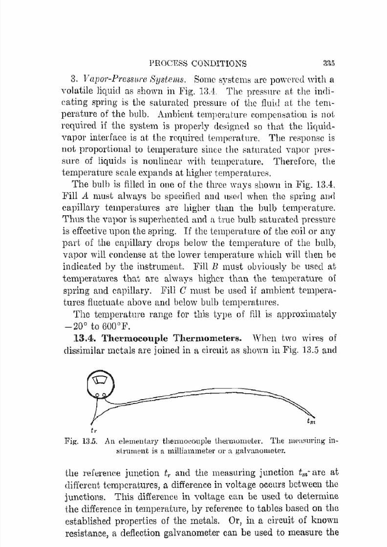
7/16/2019 Engenering Agriculture Perry
http://slidepdf.com/reader/full/engenering-agriculture-perry 355/422
1'HOCES8 CONDITIONS
3. llapor-Pj'cssnre ,systems. Some f:iystems arc powl'roc[ with a
volatile liquill as shown in Fig. l:J,.'1. The pl'essnrc at the indicating spring is the saturated prcssure of the fluid at the tem
perature of the bulb. Ambient tempomture e ( ) m f l e l l ~ a t i o n is not
required if the system is properly designed so that the liquid
vapor interface is at the required temperat1ll'c. The response is
not proportional to temperature since the saturated vapor pres
sure of liquids is l1onlillefll' with temperature. Therefore, the
temperature scale expands at higlwr temperatureil.
The bulb is filled in one of the three ways shown in Fig. 13.'1.
Fill A must always be specified and userl when the spring amI
capillary temperatures nre higher than the bulb temperature.
Thus the vapor is superheated and a true hulb saturated pressure
is effective upon the spring. I f the temperature of the coil or any
part of the eapillary drops below the temperature of the bulb,
vapor will condense at the lower temperature which will then be
indicated by the instrument. Fill B must obviously be used at
temperatures that are always higher than the temperature of
spring and capillary. Fill C must be used if ambient tempcm
tures fluctuate above and below bulb temperatnrcs.
The temperature range for this type of fill is approxirnately
-20 0to 600°F.
13.4. Thermocouple Thermometers. When two wires of
dissimilar metals are joined in a eil'cuit as shown in Fig. 13.5 and
II"
Fig. 13.5. An elp.llIelltal'Y therllloeonple thernlOrneter. The llIpasurin", in
Htl ' l lHlPut is f\ milliammeter 01' a galvanometer.
the l'efCl'ellee junction t,. and the measuring junction t,ri- are at
different temperatures, a differenee in voltage occurs between the
junctions. This difference in voltage can be used to determine
the difference in temperature, by reference to tables based on the
established properties of the metals. Or, in a circuit of known
resistance, a deflection galvanometer can be used to measure the

7/16/2019 Engenering Agriculture Perry
http://slidepdf.com/reader/full/engenering-agriculture-perry 356/422
336 AGRICULTURAL PROCESS ENGINEERING
current, for which tho voltage, and thus the temperature differ
ence, is found.The common wire combinations ami their important character
istics are listed in Table 13.1.
Table la.l T H E R M O C O U P U ~ WIRE COMBINATI< N ~
( } a n p l ~Coppm-Constu"ntltll
han-ConstantanChromcl-Alumel
Platinum-platillum, 13% ,hodium
Platinun1-plu.tinum, 100/0 I hodiuln
O o m p u ~ t t ~ o n100 Gu -55 Cu, 44 Ni
100 Fe-55 Cu, '14 Nino Ni, 9 Ot-97 Ni, 3 Al
100 Pt-87 Pt, 13 Rlt
100 Pt-90 Pt, 10 Rh
i11)prO.I:Vnate
USf'jul A]Jproximalc
'1\ mpCrailL?'C
Ranoe, 0]1'
-300 to 700
a to 1400GOO to 2200
1300 to 3000
1300 to 3000
Response,
71W pm' OF
0.0232
O.02!l20.0231
0.007G10.00(;(;0
For higher nCCU1'[lcy, [ I null mcthod using a potentiometer is
preferred. A standard voltage is produced on the slide wire shownI I I Fig. J3.6. The contact point on the rheostat is then mov('rl
Fig. 13.6. A potentiometer used for reading temperatures with thermo
couples.
until the galvanometer shows a null reading, thus indicating that
no current is flowing in the external circuit and that the voltage
resulting from t", - t,. is equal and opposing that across the por
tion of the slide wire Em. Consequently, the temperature differ-

7/16/2019 Engenering Agriculture Perry
http://slidepdf.com/reader/full/engenering-agriculture-perry 357/422
PROCESS CONDITIONS 337
ence til< - t,. can be represented by the position of the cont.act
point. Since the reading is made when no current is flowingthrough the thcrmocouple leads, standardization of the length and
size of the wires and type of junctions, i.e., of the resistance of
the external circuit, is unnecessary.
The indicator of a p y r o l l l e t ( ~ r is gmcluated in milliamperes or
directly in degrees if u standard reference temperature is used.
The potentiometer i" graduated ill millivolts or in degree;,; if a
standard l'efcrenee temperature is used. A stanellLrd reference
temperature is a fixed temperature sLIch as 32°F. C0l11111creial
instruments are frequently fitted with eompensating devices,
which automatically adjust the circuit for variation of t,. and
thus eliminate the need for consideration of tr when using the
instrument. The accuracy or reproducibility depends upon the
consistency of the wire eomposition. Usual accuracy in terms of
degrees per millivolt is ;f to 1 per ceut. All the couples can be
used satisfaetorily down to about _cl00°F. The response of
platinum couples at low temperature difference is too small for
acceptable use. The temperature-millivolt relationship is not
quite lineal' for any couple. Therefore, calibratiun data appro
priate to the temperature range and reference temperature must
be used.
Defieetion instruments are simpler but less aeCUl'ate thun null
instruments because of possible variations in eircnit T l ~ s i s t a n c e .By Ohm's law, the current in Fig. 13.5 is
(13.1)
From Equation 13.1
Em/Eg = Rm/(Rrn + Rc) (13.2)
whero I = current, amp.
Eg = voltago generated by thennoeouple.
Em = voltage at instrument.
Rc = resistance of external circuit, i.e., eouple and leads,
ohms.R", = resistance of instrument, ohms.
Thus, by equatioIl 13.2, the higher the resistaIlce of the instru
ment, and the lower the circuit resistance, the closer the measured
voltage is to the voltage generated by the couple. A given in-
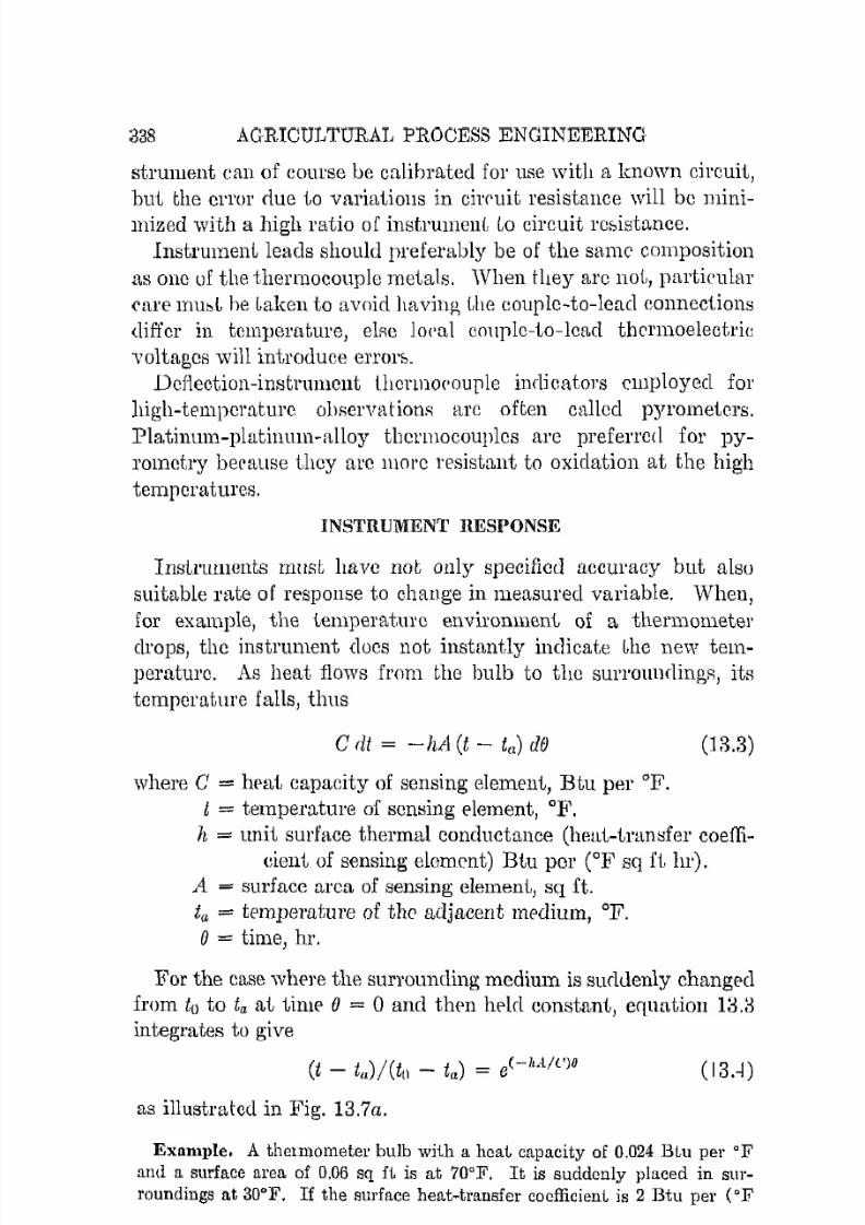
7/16/2019 Engenering Agriculture Perry
http://slidepdf.com/reader/full/engenering-agriculture-perry 358/422
338 AGRICULTURAL PROCESS ENGINEERING
st.rUluent can of course be calibrat.ed for use with a known circuit,but the error due to variations in ci1'('uit resist.ance will be minimized with a high ratio of instrUlnenL LO circuit rCtlistance.
Instrument leads should preferably be of the same composition
as one of the thermocouple metals. When they arc not, pal'tieulal'
earE' mUbL he Laken t.o avoid Juwing the couple-to-Iead connectionsdiffer in temperature, else lo('ul c011ple-to-lead thermoelectric
voltages will introduce errorf>.
Deflectioll-instrulllent ihenno('ouple imjjeat.ol's employed for
high-tempcrature oilRervntionR arc often callcel pyrometcrs.
Platinum-platinum-alloy thermocouplcs are preferred for py
rometry becallse they arc lllore resistant to oxidation at. the high
temperatures.
INSTRUMENT UESPONSE
Instruments lllllSt have not only specified accuracy but also
suitable rate of response t.o change in measured variable. When,
for example, the temperature environment of a thermometer
drops, the instrument. docs not instantly indicate Lhe new temperature. As heat flows from the bulb to tho surronndingR, its
temperature falls, thus
C rtf = - hA (t - ta) dO
where C = heat capacity of sensing element, Btu per OF.
t = temperature of sonsing element, OF.
(13.3)
h = unit surface thermal conductance (heat-transfer coeili-
eient of sensing element.) Btu pOl' (OF sq I i h1').i t = surface area of sensing element, sq ft.ta = temperature of the adjacent medium, OF.
IJ = time, hr.
For the ease where the surrounding medium is suduenly ehangpcl
from to to t" i1t time IJ = 0 and tllPn lwlrl oonstant, equation 13.3
integrates to give
(t - t,,) / (to - ta) = e( -ltA/(,JO ( 13.-1)
as illustrated in Fig. 13.7a.
EXamlJle. A thelmometer bulb with a heal, capacity of 0.024 BLu pel' of
and a surface area of 0.06 sq f(, is at 70°F. I t is suddenly placed in Sl1I'
roundings at 30c F. I f the surface heat-transfer coefficient is 2 Btu per (OF

7/16/2019 Engenering Agriculture Perry
http://slidepdf.com/reader/full/engenering-agriculture-perry 359/422
P l l O C 1 ~ S S CONDITIONS 331\
(rt)
(b)
oFig. 13.7. InHtrumellt response to :1 sudden tempern,turc dmnge (a) and
Lo a lillerlr tempm':dure change <b).
sq i t hr), what time will be required for the bulb to be within 2°F of the
new surroundings?
(32 - 30)/(70 - 30) = e- (2 X O.Uli/O.(24)o
IJ = -1/o.GOln G.05 = 0.13 hI' or 313 min
13.5. Response to Lineal' Cbange in Air Temperature. In
this case, the bulb and surroundings arc initially at to. The sur
roundings smldcnly start to rise at b degrees per hoUl', thus
fa = to + be (13.5)
Substitution of /" from equation 13.5 into equation 13.3 and i n t e ~gmtion yields
t = to + be - b(G/hA)(l - e-(lut/c)O) (13.6)
Equation 13.6 is illustrated in Fig. 13.7b. As time goes on, the
exponential term approaches zero. The bulb then differs from
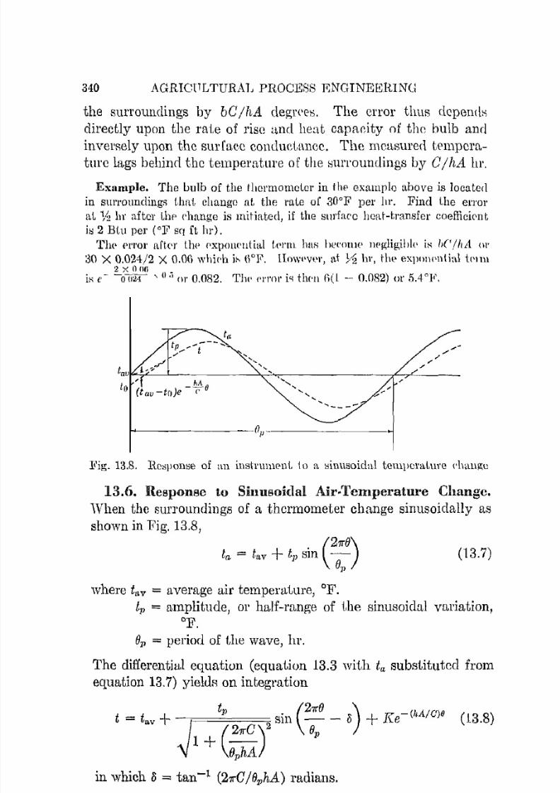
7/16/2019 Engenering Agriculture Perry
http://slidepdf.com/reader/full/engenering-agriculture-perry 360/422
340 AGRlClTLTUHAL PROCESS ENGINEERING
the surroundings by bCjhA clegr('cn. The error thus d e p e n d ~directly upon the rate of risc tincl heat capar,ity of the bulb and
invel'sely upon the surface eondudnnee. The measured tE'mpcrn.
tUfc lags behind the tempemture of the :;urrounclings by CjhA hr.
Example. The bulb of the thermometer in the example above is locatec]
in surroundings that change at. the rate of 30°F pel' hr. Find the error
at Ill' after Llw ('hange is mitiated, if the slIrfaC'e heat-transfer coeffici011t
2 Btu pel' (OF sq ft In).
'I'll(' 1']'l'or aft(,J' Uw ('xPOll('llt itt! If'l 'lIl ha R heeoll lP nrp;ligihlc' is /,(' / Ii A ( \ l '
80 X 0.024/2 X 0.0(\ whif'h ()oF. lImvPVl'l' , ttt hI', tlll' CXj)()1\I'l\tial tl'llll
2 X Ollr.
is c- -0024 ,(I •• Ol' 0.082. TIll' C'ITor thc'll ()(l - 0.(82) o r .5.4°F.
11'ig. 18.8. ltclljloilSe of an instrunl0nt j 0 a ~ i n u s o i d 1 1 1 temperature d l ~ U I ~ C
13.6. Responsc to Sinusoidal Air-Temperaturc ehangc.
When the surroundings of a thermometer change sinusoidally as
shown in Fig. 13.8,
ta = tav + 1' sin C ~ O )where fav = average air temperature, OF.
t1' = amplitude, or half-range of i,heOF.
01' =: period of the wave, hr.
(13.7)
sinusoid[tl variation,
The differential equation (equation 13.3 with ta substituted from
equation 13.7) yieltls on integration
t ~ t .d JI + ~ g _ f l i n C : -,) + K,-(W'''' (13.8)
O1'hA
in which 0 =: tan-1 (27f'C/fJ1'hA) radians.

7/16/2019 Engenering Agriculture Perry
http://slidepdf.com/reader/full/engenering-agriculture-perry 361/422
PROCESS CONDITIONS 311
]{ = a constant of integration, which is evaluated bv suhstitut-
ing values of t and ta when (j = O. .
The last term in Equation 13.8 dies out as time progresses.
A.£ter this, equation 13.8 resembles equation 1:3.7, except for the
decrease in amplitude and the lag. The amplitude ratio
ltV1 + (27['C /fJplu.t) 2 is usually of more COllcern than the lng.'rlle lag, which is expressed as a time angle Ii is cOJlverted to hoursby multiplying by 01,/27['.
Periodic temperatures that nre not simple sinn waves can he ex
pressed !Ul a Fourier series, and the response to each harmonie canbe found by equation 13.8.
Example. Thc blllh of the pl'cviou8 examples is used to mCl\SIU'e a
sinusoidal temperature having a period of hI' and a range of 10°F
Up 0= 5). Predict the range that the thermometer will indicate and alsothe lag.
From equation 13.8, the amplitude after a few cycles will be
55 = ~ = 1850F
1 + 2.512 2.7 .
11 (211' X 0.024 )2'\ j + t X 2 X D.DG
The range, twice the amplitude, is 3.7°F. It il'l obvious that this thermom
del' represents the measured variable very poorly. Its p e r f O r n l l L l 1 r ~ { J would beimproved by d i r e ( ~ t i n g an air blast over the bulb to iIlln'el\Se the hCl11,-transff'1'
coefficient.
The lag is ta lC! (211' X 0 . 0 2 4 / ~ 1 X 2 X 0.06), which is tiS.5° or 1.2 l'adians.
The lag in hours is ( ~ / 2 1 1 ' ) X 1.2 or 0.096 hr.
13.7. Response Summary. The response characteristics dis
cussed in the previous sections are related to the heat-transfer
features of the sensing element in the expression
CIliA
This has the dimension of time and is often called the time con
stant of the thermometer in the given system.
Observations are most accurate when the value of this expres
sion is small. Therefore, the specific heat, specific weight, and
volume of the sensing unit should be small and the surface heat
transfer coeffici.ent and area large if fast response is desired.
Thus, long narrow or coiled sensing units are preferred to short
thick units. The volume of the unit should be as small as prac
tical. Thermocouples made of small wire, 36 gage for example,

7/16/2019 Engenering Agriculture Perry
http://slidepdf.com/reader/full/engenering-agriculture-perry 362/422
342 AGRICULTURAL PROCESS ENGINEERING
are highly acceptable in this respect. The surface heat-transfercoefficient is high for liquid:; or {'onclensillg vapors and instrument
response is fast. Bulb-type instruments to be used with gasesshould be gas filled if fast l"f'RpOnSe is desired.
OBSERVATIONS, PRESSURE
The devices and techniques available for measuring pressures
are discusserl in Chap. 2. Coil springs and bellows similar to
those used for temperature observatiollf; are also used for pressure
observations. TheRe clements perform ill a lllanncr comparable tothe Bourdon tube, ROct. 3.4.
Since the gage tl1be is llsl1ally connected direr·tly, or with a
simple valve, to the vessel or pipe whose pressure is to be measured, the resistance to transfer of energy here is negligible, so
that a response analysis similar to that developed for the thermometer is not required. Where frequency of pulsution of pres
sure approaches the natural frequency of the gage mechanism as
a spring-mass system, serious vibration occurs. This can bereducer] by throttling with the gage valve. A routine seheclule of
checking the gage response ::;houlcl be adopted in such a case, toavoid having a gage bc('ome i m ~ e t i v ( ' from plugging of the nearly
closed valve.
OBSERVATIONS, RELATIVE HUMIDITY
Relative humidity,de
fin cd::md
discussed in Chup. 10, can beobserved by four methods.13.8. Wet.Bulb Psychrometer. The wet-bulb method of ob
serving relativc humidity is discusscd in sects. 10.6 and 10.11. I t
is the most frequcntly used procedure and, in view of its simplicity, one of the most accurate.
The accuracy of Lhe relative-humidity observation is de
pendent upon the accuracy of the temperature observations and
the accuracy of the tables or charts £1'0111 which the values aretaken. An error of less than 1 per cent of relative humidity canbe expected when careful observations are made. This procedureapplies between a wet-bulb temperature of 32°F and a dry-bulb
temperature of 212°F. Wet-bulb observations can be used to
determine air conditions above 212°F, even though relative

7/16/2019 Engenering Agriculture Perry
http://slidepdf.com/reader/full/engenering-agriculture-perry 363/422
PROCESS CONDITIONS
humidities lire low here. I t is basically acceptable )lelow 32°F,
but tcmpernturcs ill this region must be read with exceptional
accuracy to secure reliable results.
In cases where the wet bulb nlay be below 32°F, cnrc must be
taken to distinguish between a wet bulb ami an icc hulb. A", the
temperature of the wick drops below 32°F, ale water tends to
subcool. I f a minimulll tClllperatlll'e is reached without freezing,
wet-bulb tables arc valid. Howcver, if freezing occurs, the mini
mum wet hulb may not be att!lincd, and the tempcratlll'c ri:;es
quickly to 32°F. Observation must be contiuued until a now
minimum i8 reached, the ke-bulb tcmpcrat1ll'e, fm which iee-Imlbtemperature. tables are a vailahle.
13.9. Dew-Point Device. T11e dew-point temperature eUIl IJC
used to establish a state point on the psychrometric. chart from
Coolant
Thermocouple formeasvring surface -+: :=1 ' " '1
temperature
Light fromstandard source
Fig. 13.9. Principle of O P ~ l ' ! t 1 · i O I l of It dew-point app[\mlllR.
which relative humidity eall he taken (sect. 10.12). The tem
perature of the dew point is observed by lowering the temperature
of a polishe(l surface to the point where ll1uisture just starts to
condense from the air onto the surface. The exact point or tem
perature at which this phenomenon starts is difficult to observe

7/16/2019 Engenering Agriculture Perry
http://slidepdf.com/reader/full/engenering-agriculture-perry 364/422
844 AGRICULTURAL PROCEHS ENCHNEEHING
with the naked eye. The procedure outlined in Fig. 13.9 will give
more acceptable results.
The light impinging on the photocell is of constant intensity;
t.hus, the photocell signal is constant. The reflecting surface is
cooled slowly by the cooling medium. At the instant condensa
tion starts, the light rays arc clisllcrst'd and the intensity of the
signal from the phoLoeell decreases. The surface temperature
observed by the thermocouple when the signal (Iecreases in in
tensity is the dew point.Accuracie::; are high. The polished surfaec must be kept ex
ceptionally clean since dirt will cause the light to disperse, thus
confusing the point of condensai,ion. The frost point may be ob
served to as Iowa temperature liS - gO°F.
13.10. Hygrometers. Many hygroscopic materials contract
ancl expand significantly when the moisture content varies. Since
the moisture content of a hygroscopic material is related to the
relative humidity of the surrounding air by the equilibrium mois
ture curve, the relative humidity of the ail' can be indicated by
the change in dimensions of the material. A rievice that uLilizeHl;uch a material is called a hygrometer.
Human hair, wood, and (·(·rtain animal tis:>ues are Lhe illo:;L
frequently used maLerial:;. Tlw ehange in length of an element
made of thel:ie materials is condueLed Lhrough a kinemu,tic chain to
an indicator.
Hygrometers arc secondary instruments and must be calibrated
against acceptable standard:>. Temperature, age, and the range
of exposure to humidity all affect the calibration. Rehttivehumidities outside Lhe appruximate range, 35-90 per cent, arc
difficult to include in a calibration and, if experienced by a eali
brated instrument, may alter the calibration. The instrument'i:l
response time is long. Variable humidities may be difficult to
follow. Carefully calibrated, used, and handled hygrometers may
give satisIactory readings for many observations. However, these
instruments must be checked and calibrated frequently if readings
of rerruisite accuracy are to be expected.13.11. Electric Hygrometer. A hygroscopic salt such a::;
lithium chloride changes its moisture content with relative humid
ity according to its equilibrium moisture curve. Therefore, an
inert material mixed or coated with a salt such as lithium chloride
will vary in elcctrical conductivity wiLh moisture content anci
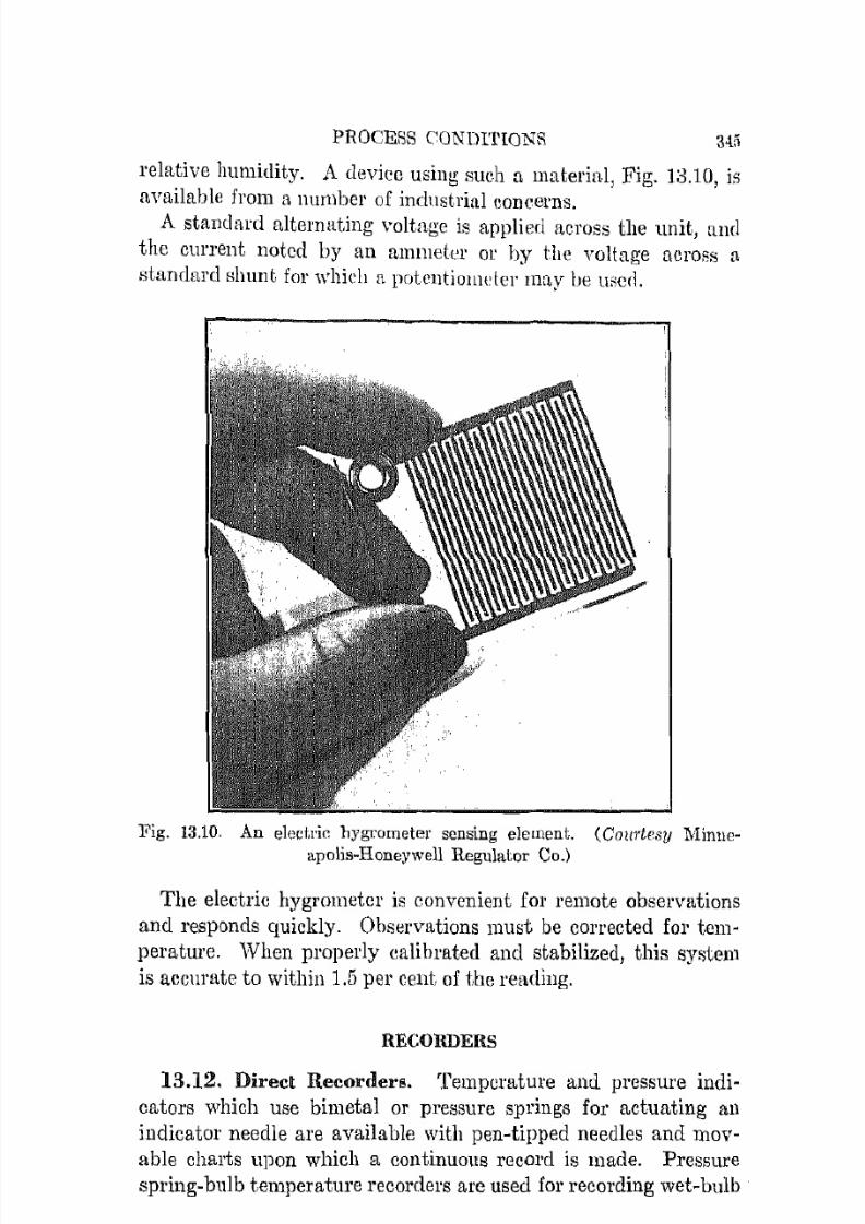
7/16/2019 Engenering Agriculture Perry
http://slidepdf.com/reader/full/engenering-agriculture-perry 365/422
PROCESS CONDfl'lONS
relative humidity. A deviee using such [ l material, Fig. 18.10, is
available from a number of industrial eOIlcerns.
A standard alternating voltage is applied across the unit, uud
the Cllrrent notcd by an ammet('r or by the voltage across a
standard shunt for whieh a pDtentiollldcr may be used.
l ~ i g . 13.10. An electric: hygrometer sensing element. (Cmll'te81J Mimw
apolis-Honeywell RegUlator Co.)
The electric hygrometer is convenient for remote observations
and responds quickly. Observations must be corrected for tem
perature. When properly calibrated and stabilized, this system
is accumte to within 1.5 per cent of the reading.
RECORDERS
13.12. Direct Recorders. Temperature and pressure incH·
cators which use bimetal or pressure springs for actuating an
indicator needle are available with pen-tipped needles and mov
able charts upon which a continuous record is made. Pressure
spring-bulb temperature recorders are used for recording wet-bulb'

7/16/2019 Engenering Agriculture Perry
http://slidepdf.com/reader/full/engenering-agriculture-perry 366/422
346 AUHICULTUR.\L PIWCE:-;:-; ENWNRERINO
telllperatures by fitting the bulh with a "sock" that Mimulatcs thr
wet-bulb t hermolllpter. Hair and wood hygrometers [Ire similarly
fitted for recording.13.13. Indirect Recorders. Thermocouple systems involve
potentials too rmml1 to oYel'comc the frietiDJl of a recorcling 8yS
tem. The galvanometer needle is m;od a8 a positioner for a
mechanical system that activateH a reoor<lel'. The millivolt ]10-
tentialmt1y a1&o be [ecl into a vacuum-tube Hystelll (fLn amplifier I
thnt contl'ols sutIicient electrical ellt'rgy Lo operate a recording
mechanism. The electrical hygromcLer haR inRufficicnt signal for
direct recording Hnd mUl:lt be combined with H secondary recordingsystem.
13.14. Characteristics. Heconlcrs luwe approximately the
same accuracy as indicators Lhat USt' a comparable mechanislll.
Recorders arc made with (Iiscs, cylilHlel'b, and rontinllous ('hartH.
Chart:> cOYCl' various Lime ranges such as 1 hI', 24 hI', 1 week,
1 month, etc.
CONTROLLERS
13.15. On-Off Controllers. Controllers or ('olltro] prucedures
lllay be Lliviclerl into two groups, (1 ) o n ~ o f f controls and (2) modu
lating controls. On-off control indicates t h ~ \ " L the medium being
contrulled fiows full or is completely shut off. A modulniing con
troller varies the rate of flow La match the deman(l. Flow is con
tinuous. Three types of modulating controls will be cliseuf;sec];
they are: (1) floating, (2) self-operating, (3) pneumatiC'.}\i{ost room thermostats, controls for refr igerators and hot-\vatcr
heaters, and switches for automatic water systems are eXaInples
of on-off control (sce Fig. 13.2). All the deviceH and mcrhr1l1isms
tliseussecl in this chaptcr are or can be fitted with various elec
trical Rwitehcs 01' valveH Lhat make Dr int[,l'l'upt a flow. The
bimetal a n ( l l n ' C S H 1 1 r e ~ s p r i n g me!'lmnis1ll8 ar[' used extensi.vely for
switch activation. Rueh devices arc qualified by the range
through which tlley can he ad.iusted, the diffcrcntial range, that
is, the difference between the on and off position, the adjustability
of the differential, and other important features such as maximum
current, rate of flow, and corrosion resistance. Thermocouple
systems can be used for eon('rol by incorporating a switching
mechanism in the indicating or recording system.
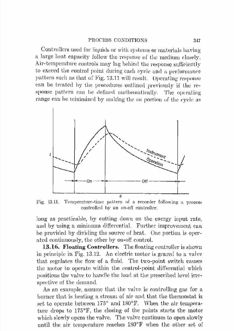
7/16/2019 Engenering Agriculture Perry
http://slidepdf.com/reader/full/engenering-agriculture-perry 367/422
PROCESS CONDITIONS 347
Controllcrs used for liquids or with systellls or rnatel'ial" il[wing
i t lnrge heat cllpaeit,y follow the response uf the mediulll c:1oscly.Air-temperatme eontrols may lag behind the l'e:-;ponse suffieiently
to exceed the (!olltrol point rlm'ing each cycle and n llcl'fonnnnee
pattern such as that of Fig. 13.11 will result. Uperating j ' l ':"j)0l);;C
e[tIl be treated by tlle JlI'oeedures outhned previously if the re
sponse pattern can be definerl mntlwlllatieally. The operating
range c:tn 1)() ll1inil1lizC'd by making the 0/1. portion uf the eyr·le as
- " " * f - - -On --/4------ Off - - - - - - t .......
H
Fig. 13.11. Tel1ljlcl'a.ture-tiuHl plLttel'l1 of II J " ( ~ ( : o r d e l " following a 1 J r o c e s ~controllecl by iU l oil-off con troller.
long as practieable, by cutting down on the energy input rate,
anI] by using it minimum differential. Further improvement can
he pl"ovided by dividing the source of heat. One portion is oper
ated continuously, the other hy on-off control.
13.16. Floating Controllers. The fluuting controller is shown
in principle in Fig. 13.12. An electric lllotOl' is geared to a valve
that regulates the flow of a fluid. The two-point switch causes
the mutor to operate \vithin the eontrol-poinL tlifferentitil which
positions the valve to handle the loar] ttt the prescl'ibed level ilT(,
spc{:tive of the demHlllL
As an example, nssume that the va[yc is eontl'ullil1g gas for aImmel' that. is heating a strctlln of air and that the thermostat is
set to operate between 175 0and 180°F. ,Vhen the air tempera
ture drops to 175Q
F, the dosing of the pointR starts the motor
which slowly opens the v[IIve. The valve continues to open slowly
until the air temperature reaches 180°F when the other set of

7/16/2019 Engenering Agriculture Perry
http://slidepdf.com/reader/full/engenering-agriculture-perry 368/422
348 AGRICULTURAL PROCESS ENGINEERING
point:> close, the motor reverses, and the valve closes slowly. ThuR
the motor slowly oscillates or "ftOllts" the valve within the setrange, adjusting the gas rate to the demand.A motor of this system il:) also wired to operate only when the
points are in ('ontact. Thus, the motor docs not operate as long
as the temperature is within til{' tlet range. "Vhen iJlO low pointis contacted, the motor operates the valve to bring the systeminto balance; the lll()tor op('[·[1Lo;.; as long ns the points are in eon-
Sensingbulb
Fig. 18.12. Hl:heml\tic lll'incilll" of opel'ation of floating rontl'oli('l'.
tact. The upper eontact operates the motor in the l'ever;.;c diree
tion. This system itl used more frequently than the first system
discussed.
Care must be used in adjusting the valve-movement rate to therate of temperature change of the system. A valve-moving mechanism which decreases the rate of valve movement as the set point
is approached provides i t smoother performance curve.13.17. Self.Operating Controllers. Controllers of this type
(Fig. 13.13) are used cxtentlively because of their simplicity. Thebulb is fillcd with a fluid whieb has a steep vnpor pressure-tem
perature curve through the operating range so that a maximum
valve movement will result for a minimum change in control temperature. The alcohols, ethel', and various refrigerants are used
to fill the bulb. Valves of this type can be used to control pressure
by replacing the pressure bulb with a connection to the pressure
heing controlled. Note that if the temperature (or pressure) ex
ceeds the {'ontrol point, the valve will close completely.

7/16/2019 Engenering Agriculture Perry
http://slidepdf.com/reader/full/engenering-agriculture-perry 369/422
PROCESS CONDITIONS
A temperatl1re variation of approximately 5°F will operate
most valves through their entire range. The response character
istics can be determined by the procedures cli8cussed earlier in the
ehapter if the valve-shaft friction is not great.
Fig. 13.13. A lH'oH:,-sedioll drawing of a ~ e l f - ( ) j J e m t i l l g controller. (Cour
tesy The Powers Rl"glliator Co.)
13.18. Air-Operated Controls. An air-operated control sys
tem is shown schematically in Fig. 13.14. The air ~ y s t e m is the
most versatile of all the control devices. Since the force or energy
required to regulate the control air pressure is small, this system
can be combined with any of the indicating devices discussedearlier in the chapter (except the glass thermometer). The sensi
tivity and rate of response of the instrument can be adjusted
through wide ranges by simple adjustments. Thus, it is possible
to balance an instrument with the rate of response of a. system
so that maximum performance will result. The sensitivity nan he
adjusted to as low at:) O.l°F 01' equivalent in pressure or relative
humidity. Since the ail' motor is basically independent of the
control mechanism, air-operated controls can be adapted to a
great variety of processes. Availability varies fro111 simple sys
tcms with fixed characteristics to systems that are completely ad
justable to the characteristics of the process being controllcd and
that control at a fixed set point irrespective of the magnitude of
the load.

7/16/2019 Engenering Agriculture Perry
http://slidepdf.com/reader/full/engenering-agriculture-perry 370/422
350 AGRICULTURAL l'iWC'ERR ENGINEERING
111213141516171819363738
10
9
8 - - - - = < : I ~ \ . , ( 1 I f7 - - - - -Q ' 1A ; : : JC " "
6 _ _ - - - - - n r o ~ ~ ~ ~5
4--_-1// /I I I L _ ~ ' , . r . ~ ~3
2 - I t ~ I - - - - " \
70
63
62
61
1-
39
_---- - - I t - - - 45
, - - - - - - - 1 1 - - - - 4 6~ g t = 4 7 8
49= : : = - - - - - - 5 0
51
57
58
20 Ib air supply
--Process59
60
Fil,!;. 13.1-1. Schematic diagram of a ~ i l 1 1 1 1 1 e Ilir-opcl'al(ld (·untrol HysLcm.
When ~ t e a d y - s j , a t e e o n d i i i o n ~ exist, air is bb l from liJw 311 through the
orifice> aI, 14. The p r c : , ; ~ u r c in linp 3H [ J o ~ i t i o n 8 t.he ball valv!! at 48 so that
!I fixf'd pres,lllre is produced :ll, 58. Thus, t.ht' valve (59) is lIPId at it fixed
opening. A chauge in LCinperaturc (61) will eause a e h ! l n ~ e in the orifice
clearance (14), and the pressure in line 39 will change. Tho bellows (51)will adjust the ball valye (48). The p l ' e ~ s u r e aL 58 will "hange, and the
valve will move the proper amonnt to reaclj ust the process condition.
( C O t ~ r t e 8 Y Taylor Instrument Co.)
7/16/2019 Engenering Agriculture Perry
http://slidepdf.com/reader/full/engenering-agriculture-perry 371/422
PROCESS CONDITIO.KS 351
High eost is the chief dis::1.cinmtage of thi" (·(mtrol. T h t ~ more
sensitive instruments may require expert attention to maintainproper performance.
UEFERENCES
1. Behar, M. F. The Handbook oj M C I I . ~ l m ) 1 J l l ' l i t . onrl Control. 111,,1\'\1-
ments Publishing Co. Hl51.
2. Dunmore. F. W. An Electrie H:I."!!;romf'lr,r awl lls AJiflli .alirm to RadiolYldeorology. .T. RC8l'n)'ch Null. Bur. St(lllrlord" (Rc.w;((l'ch P((}II'i'
11(2) 20 :723-744. 193R.
3. E('kman. D. P. buI ld rill I in, lrwllrn/([/ io1!. \ v i l l ' ~ ' . 1050.
4. l"nrringl;oll, C. H. Ji'umlll/i1Clllld8 of Allfonwlie Control. \ V i l p ~ · . HJ51.
5. F'ulldanum!ols of P ( ( ' . ~ 8 1 ( I ' C (1)/(1 ' l 'nllprra/.-i l l 'r: T 1 1 . ~ I , ) , I l I I W / l t 8 . Delmar.
1947.6. hl.ltn(.'men/,q ((lId ProCf'sS Conll'ol. Delmar. 1045.
7. Smit.h, R. S. Autuillotir- CmilmZ Enuinecl'ill(/. McGraw-Hill. HH4.
7/16/2019 Engenering Agriculture Perry
http://slidepdf.com/reader/full/engenering-agriculture-perry 372/422
C HAP TER 14
Cost Analy sis
NOMENCLATURE
.A = annual replacement reserve 01 ' annuity, dollarR.
i = interest rate, per cent.
1 = expected life, yr.n = a period of time, yr,
l ' = anllual depreciatioll ralp, per cent.S = cost llew less salvage vlJ,lue, dollars.
The commercial sucress or failure of a processing enterprisc
depends, naturally, upon the difference between cost of production
and income. In turn, t h i ~ diffcrential depends upon the integratedperformance of the individual units. The over-all economicanalysitl and man\\gement of a. plant is a highly skilled process
and involves procedures that are too complex to be completelytreated here. However, the elcmentary principles and procedures
will be discussed relative tu unit opcra.tiom; in order that the
engineer will bc able to e ~ t i m a t e the vnriom: costs of simple
processes.The machine of the highest energy efficiency may not be the
most satisfactory machine economically. The added ail' volumcfrom a larger fan may give better pcrformance but not be worth
the extra cost. An automatic machine may be expensive but soreduce labor costs that the unit product cost is less. A new sorting device may produce a beUer-quality, more valuable prod\lct,
but the increase in nnit cost may he grenter than the increasedvalue of the products at the existing price structure.
This phase of engineering is too often disregardcd. Carefulattention should be given to costs since they are one of the mostimportant factOl's in any engineering problem.
GENERAIJ CONSIDERATIONS
It is usually advisable to detcrmine the cost analysis on a unit
product basis. For example, what is the cost per quart to own352

7/16/2019 Engenering Agriculture Perry
http://slidepdf.com/reader/full/engenering-agriculture-perry 373/422
COST ANALYSIS
and operate a certain milk-bottle washer? What is the cost per
hundredweight to elevate: sacked lin'fitor'k feed with a bag ele
vator? How ll1u('h does it cost to quick-freeze 100 Ib of meat?
Note that the total production east per unit would he the sum of
the unit operation costs.
I t is not always advisable for each unit operation to function
in the most economical manner. I t is the: accumulated per
formance of a series of o p e l ' : \ t i o n ~ which p r o d l l ( ' e ~ a distinct end
point in which we arc interested.
Unit costs are elOticly related to ~ t l l d affeeted hy the "flow" pro
l'edure in a plant. This topic will be treated in the next chapter.
ITEMS OF COST
For convenience, the total ( ' o ~ t pOl' ll11it is broken down into
(1) fixed and (2) operating costs.
14.1. Fixed Costs arc tho:,;c that arc ll:,;mtlly not directly re-
lated to the amount of use; they include;
1. Depreciation.
2. Interest on the investment.
3. Housing.
4. Taxes and insurance.
The depreciation of many standardized machines for standard
ized procedures may be a function of lise. Steam boilers, choppers,
and drag elevators depreeiate because of over-all wear. However,
since they can be repaired, the length of service can he extended.
This is discussed in detail under "life expectancy."
14.2. Operating Costs are those that are directly related to
use; they include;
1. Fuel, power, and utilities.
2. Labor.
3. ]Vlaintenance.
A machine or unit operation includes the device that produces
the result and the power unit that drives the device.
14.3. Depreciation. Depreciation may be defined as the
decrease in value of a piece of 1)l'Opel'ty during a period of time.
The decrease is considered from the standpoint of amounts to be
set aside each year in order to recover the cost of the unit at the

7/16/2019 Engenering Agriculture Perry
http://slidepdf.com/reader/full/engenering-agriculture-perry 374/422
: ~ 5 4 AGlW'TTLTURAL PROCEHH ENGINEERING
end of ib, l l ~ d l l l l i f t ' . Tllit-i pro('eriure is frequclltly callt'cl amorLi
zation. Tldt-i dccl"enfie, Wlllf'h is u ~ u a l l y ciotel"mill(:,d on a yearly
basiH, is charged to the proclu('tfo procl\l['etl. This ('llarge is legiLi
lU[l.te, Hince tItp piece of property, which may be a machine, Imil(l
ing, ur similar unit, is pxpend('cl only in order tu produce a pro( IUd.
A diHtinction !:'hould be noLml between depreciat('(l value, actual
value, reRale value, and tnxabk value. 'rhe depreciated valup,
sometimes called the book valne, is the ('Urrellt value ftS shown
1,y the books of the ('OI1('ern. The actual va,lue is lHtKE'cl upon the
vtdue which the '-mit adds to the product. The resale value is the
beht p1'i('o Lhat could he 1'o('oiy('(1 for tho unit, on the open market.
A pieoe of equipment, a hammer mill, for example, may luwe eost
$600 new. Ittl prci:lent resalE' value may be $470. However, its
tleprrciaterl or bouk value may be only $21)0, hut it lllay be worth
$650 to the en t er)11'ifoe. n is gPl1Prally advisable to rnaintain a
cleprceiatecl -value le"s than the actual vulue. Thus, c](:'ercnsecl
eonSUll1er deman(l or other rlepressing factors such as forco(1 price
reduction do not materially upset the O\'er-all stability of the
enterpriEle. The taxable value it-> a base value used for ralcul[l.Lingtaxes and may not be the sume as either book 01' [l,ctual vtilues.
14.4.. Straight-Line Depreciation. The simplest and l110:,t
widely used procedure for determining the annual depreciation
charge is UlC straight-line method shown in Fig. 1<1.1. The de
preciation charge pel' year is
(Cost new - Salvage value)/Totnl E'xpC'cted-life in years (14.1)
The salvage value it! the junk or ret-iale valut' nt the ene! of the
useful life of the maehine.
TIlE' annual clepl'l'eiation as dE'terminee! by the Eltraight-line
method if tt('('ullmlated rluring the life of the unit is sufficient to
replace it at the end of ib ut;efullife. This procerlure is not too
realistic because the accumulated reserve is not credited with
interefot.
A husinesslike, i:louml pro('e<iure which is f1'equently used is the
accumulation of a si1lking, fund on an annuity basis. A certain
amount that is not as large as the annual depreciation basod upon
the straight-line method is put abide each year. The aceumulated
all1o\.mt with intereElt that compounds annually is sufficient to pro
vide replacement at the end of tho useful lifo. The amount A

7/16/2019 Engenering Agriculture Perry
http://slidepdf.com/reader/full/engenering-agriculture-perry 375/422
COST ANALYSIS 355
that must be placed annually (cnclnl year) at ("olnplltlllfl interest
i for 11 term of l years equal to [lie I'xpedcd life of the unit tocreate an amount,') i:s:
iII = 8 - - - " ~ - .
( 1+0 [ - 1(11.2)
.':) is equal to the cost Ilew less I.1Il1 KHlvage. \·:dnc. This is a pl'O
cedure that can be lIsed t.o j)roviflc n sinking fund large cuoughto rCC'OVPl' the (:o"t of the uuit by the end of its useful life.
S:OJ
; 6 0 r - - - - - 4 - ~ ~ - + ~ ~ ~ ~ - - - - ~ - - - - ~'"u
'0
- 4 0 r - - - - - ~ - - - - - + - - ~ ~ ~ ~ ~ ~ r _ - - ~....rf
° O : - - - - - ~ - - - - ~ - - - - ~ ~ ~ L L - - - - ~20 40 60 80 100
Per cent of expected life
Fig. H.1. Dep],pei;ll:ion of a unit, by straii1;ht-liM, fixed-pcrccnl.agc-of
Tll'csen1-va!ue, and jU'8Renl-worlll nwtllods (a t two j l C l ' f ' 0 n t [ t g ( ~ l'fllp;;).
Consider a $1000 unit expentc(l to last 10 y e ~ u ' H (no salvugc
value). The annual depreciatiun would $100. The annual
annuity ;-1 would be
0.0"1A = 1000 - 10 = $83.38
(1 + 0.(4) - 1
Thus, only $83.33 would have to be placed aside annually to
accumulate the needed amount in 10 years.
In a going concern containing many units, funds made Hvaihtble
by straight-line-depreciatiun methods are reinvested in the bmii-

7/16/2019 Engenering Agriculture Perry
http://slidepdf.com/reader/full/engenering-agriculture-perry 376/422
356 AGRICULTURAL PROCESS ENGINEERING
ness. This not only proviues a general depreciation reserve but
also perlllits i t satisfactory return on funds that are providcrl for
replacement.
14 . 5. Other Methods for Calculating Depreciation. Of a
number of other mcthods that are sometimes used for rletcl'mining
the depreciated value, and of course the lmmu\l depreciation, tWll
will be discussed.
1. The Fixed-PercBntage-of-Pl'esent- Fallle NIBlhod is some
times uSNl where it is a(lvist'\,ble Or l\esimhle to depreciate the ullit
at a fustcr rate when ncw than WhE'll it becomes older. Each
year, the annual clepl'cciai,ion it; n ('onstan\' l1E'l'ccnLage of the
depreciated value at the heginning of the year. In Fig. 14.1 the
constant percentage curYe is prodlH'cd by derlueting 16.7 per
cent of the value at the heginning of each year as the annual
depreciation.
This proceuul'e C[111 he uscd under economic hazards where it isadvisable tu depreciate tbe unit at a iaHt rate. For example, !t
dairy-products processor may purchase i t homogenizer for fluid
market mille I f the demand for homogenized milk is unstable
and there is a possibility that ('onditions may clmnge in the neal'
future, thus reducing, the sales of the product, then this deprecia
tion procedure would be !tllvisablp.
Thp constant percentage curve, Fig. 14.1, is lJar-;pd upon the
salvage value and h, expressed thus:
Cost new (1 - r) I = Salvage valtl("
whel'e l' = annual depreciation rate, pel' eont.
l = expected service life, yr.
(14.3)
After the value of }' iH determined on the basis of new cost, ex
pected service life, and salvage value, Lhe vltluc at the end of any
Yl:'ar n would be
Value" = Cm,t new (I - 1')" (14A)
Both annual interest on inve:;tment and annual depreciatiull
are higher during the first few years of u::;e than later. COllse
quently, the not operating return during tho firHt years of llse
must be relatively high to offset these high costs.
2. The Present-Wol'th JvIethod of depreciation is recommended
where the factors involved are relatively stable. This would

7/16/2019 Engenering Agriculture Perry
http://slidepdf.com/reader/full/engenering-agriculture-perry 377/422
COST ANALYSIS 35i
imply that the east new \"ould not vary materially (lver a period
of years, t.hat the estimated length of sel'viee would be reliable,
unci that the salvage value could be estimated closely.
The p l ' e s e n t ~ w o r t h method is based upon the sinking-fund
procedure for providing a replacement reserve, and it may be
described as a method of arriving at the present worth Or value
of expected returns. At an interest rate 1:, the income for l yean;
from an investment A compounded annually is
Incomel = A[(l + )1 - 1J (14.5)
This return could be assumed to be from a machine, process, orplant as well as from a like sum of money. The present value of
this investment 01' expended value of the machine is
Present valne" = ~ 1 [ ( 1 + i)n - 1] (14.£))
Therefore, the present worth or value of expected service or r e ~turns is the difference between 14.5 and 14.0. Dividing this by
the total expected income (14.5) and multiplying by 100 gives the
following expression(l + i)" - 1
Condition pel' cent = 100 - lOO 1 (14.7)0+1:) -1
This is known as the condition per cent, which, when lllultiplied
by the cost new, gives the present value or, more exaetly, the
11l'eScnt worth of expected returns.Note (Fig. 14.1) the p r e s e n t ~ w o r t h curves for two rates of
int.erest. These curves yield an annual depreciation which is
small at the beginning and increases as the unit gets oldcr. Note
that the depreciation for the first year is the amount of the
annuity which must be placed annually to provide a replacement
amount at the end of the useful life.
The sum of the annual depreciation at any age and interest onthe depreciated eost at that age is constant and is equal to
Cost new
(i+ -- i 1 )
(1 + i) - 1
(14.8)
This feature is specially noteworthy and acceptable since this sUm
by other methods is higher during the earlier years of life.
14.6. Life Ex.pectancy. Depreciation must be based upon au
estimated or assumed 1.1sefullength of sel'vh'e. Suitable values are
7/16/2019 Engenering Agriculture Perry
http://slidepdf.com/reader/full/engenering-agriculture-perry 378/422
3 , ~ 8 AGIUCTTI/rUHAL PIWcrnS8 ENn£NI£fGlUNt;
frequently difficult to secure. Many studies have been made of
tl1l' expected l l l;dul life 01' life expectancy of inchlRtrial and agricultural equipment. The mortality curve" of piecet; of industrinl
anll ag,l'icnltuml equipment are ~ i l l 1 i h \ l ' to !nlllUm lllorLl\lity curves
w;l'd by Iifp inslll'ance companies. This if;, especinlly true for those
e;Lanr!anlizec! pieces of equipment used under conbistent conr1itions.
Hnilrflad rolling stock, power-gc'nC'rating equipment, nml meters
me eX[l,Inllles. Many picces of agl'ieultuml equipment also show
this charaeteri::;tic [mil the expected life of en,ch determined by
:systematic studies is generally reliahle when Lhe piece of equip
ment is not affected by unforeseen ltazal'dH.
Factors that, may cam;e the actual uscfullife to be shorter than
the estimated 01' <:'xpected life arc:
1. Obsolenee.
a. Teclmolog,ieal improvellwlli.
b. Improvement in machine c\('sign.
2. Change in supply 01' consumer demand.
3. Chango in production factors, "mch as:a. Labor.
b. Power.
c. Transportation.
T ~ 1 b l e 14.1 liHt8 some c'xj)('cLl'rl-life v a l u o ~ [01' a ::;cleekd nnrnbcl'
of unite; of equipment. The alllount of usc lllay affect the ox
peetecllife of a unit. However, since sysienmtic maintenance and
repairs can prolong the usefulness of (1 unit, an eX(1ot, life expeo
taney is difficult to provide. The mtmager mUi:lt lmhmce annual
repair and maintenanrc costs against Lhe added llep1'eeiation of a
new unit. Sitwe oosis vary, eaeh case must be handled separately.
COJll:,iclernblc judg,Illout lllllRt be exercised ill ::;elerting an ex
pectancy value £01' a specifin casC'. The hest IH'ocedul'c I::; to
in::;peet the ullit after a 11e1'iol1 of yen.rs, aSbiglling new and more
reliable values. A Rtrnight-lino ilopl'orintiull curve which wus re
evaluated is shown in Fig. 14.2. NOi,e that the expected lifo and
salvage value have untIl ilC'cn changed. This iR n recollllllendedprocedure since currenL conditionH HS indicated above lIlt1y changethe length of thc useful life u,s cstill'mtcd initially.
14.7. Interest on Investment. Interest on investment is
charged against the piece of equipment as an initial or guaranteed
return to owners and investors, such as bond, stock, or mortgage

7/16/2019 Engenering Agriculture Perry
http://slidepdf.com/reader/full/engenering-agriculture-perry 379/422
COST ANALYSIS 359
Tuble 14.1 EXPECTED S I ~ R V I C g LIFE OF SOl\IE UNITS
USED IN l'ROCESSING
Un£t
Feerl grinderFrame buildingBrick buildingBoiler and RottingsPumps -
Oil burners
Water softenersRefrigeration Il1tLchincsAir COJllllreSSorRConveyors, belt
Conveyors, chainConveyors, screwCrushersDriersElevatOl's, bucketF:1n8
FurnacesSepanttors, centrifugalMotors, tt-C
Packing machinery
100 ~0
E:l'pedcri 8ervire
L1je, !II'
III
20:18
12
7-107
81a
20-2:3Hi2010
12-172020
~
10-20
2018
2017-20
"-Point of _ "
evaluation
20
Source
Davirli;on allrl Hrnclersi)ll 4
HnadllllUHc and Henderson I;
Roadhuuse and H e n r l e r ~ ( J l l G
Roudhollse unf[ Henderson"Roadhouse and Henderson 6
Hoadhouse and Henderson U
Roadhouse and IIenrlersoIl &
Roadhouse llnd Henrk,rsoll G
J. I-I. Perry r,
.T. H. Perry [,
.J. H. Perry 11
.J. H. Perry 5
.J. H. Perry r.
J. H. Perry"
.T. H. Perry"
.J. H. Perry r,
.J. H. Perry"
.T. H. Perry r.
.J. H. Peny 5
.r. H. Pcrry 5
~ ~ ~- ~...' ..
"-Q)Q)
i\ i i\ i ""'"UJiIJ Ill::>:;::; "'''' t : >-
>- ;z: -ro:5 -<l l " ' :>
"'''' VIVI
00 20 40 60 80 100 120Per cent of initial expected life
Fig. 14.2. Straight-line depreciation showing the result of l'ee"Ulllu,tion.
7/16/2019 Engenering Agriculture Perry
http://slidepdf.com/reader/full/engenering-agriculture-perry 380/422
360 AGRICULTURAL PROCESS ]!}NnINEERING
holders with a contract rate of interest on the investment. ·When
management is the owner and the piece of equipment is nol mort
gaged or otherwise encumbered, interest is still charged to theunit as minimum or guaranteed return to the owner. I f a unit
cannot return marc than would be received if the money in
vested were loaned at the cUl'rent rate of inlercst, then its use if)
questionable.
[nterest on investment is determined in thrce different waYR.
Consider a unit costing $1000 and expected to last 10 yr with
the current rate of interest being 4 per cent.
1. Interest on Depreciated Value. The depreciated value atthe beginning of the year is ubed aR the principal. For example,
during the third year the above unit would Jw worth $800 and
the interest would be $32. ~ i m i l n r l y , the value during the eighi,h
year would be $400 and the interesL, $16. This lWocedure if;
recommended when the unit is of major imparLance or otherwiRe
is separate and distinct from oLher units aml rctaim; its idcntiLy
during it.s entjre life. A Bteam boiler, diose] engil1c, 01' large
hammer-mill would fall in this clm;s. There might he only oneof each in any plant, and it would be replaced at the end of its
useful life.
2. Interest on Half oj Cost New (Used with Straiuht-Line De
preciation). In this way the principal usee! each year is half the
cost or $500, referring to the above example, and the annual in
terest charge would be $20. This is the most frequently used
method and the most practical for most plants. I t is particularly
adaptable for enterprises where the identity of each unit cloes notneed to be maintained and the interest charged eventually reverts
to the enterprise itsclf. A further (listinctive feature is that all
the pieces of equipment do not need to be replaced Itt the same
time. The enterprise as such may be morLgaged, but the indebt
edness applies to the enterprise as a whole rather than to individ
ual units or machines.
3. Interest on TotaL Cost New. Infrequently, the annual
interest charge is based upon the cost new. This may be j u s t i ~fled in cases where the expected life cannot be well defined or
peculiarly hazardous conditions exist. It is not l'Qcommended
for general use,

7/16/2019 Engenering Agriculture Perry
http://slidepdf.com/reader/full/engenering-agriculture-perry 381/422
COST ANALYSIS 361
14.8. Housing. I t lllay or may not be necessary or advisable
to include a fixed annual charge fur housing. It is usually cus
tomary to handle housing as It separate and distinet item entirelyseparate from the production units. In spite of this procedure,housing is a direct result of the necessity for protecting the equip
ment. Consequently, it should be prorated among the various
duties that it performs which would be storage, office and shop
space, space for equipment, supplies, miscellaneous.
The itemo; of cost of the housing unit cau be broken down in
tbe same manner as for a machine, calcubted on a yearly basis,
and then prorated on the basis of floor area, structural volumeoccupied, value added to the product, or eost of the unit. It is
usually advisable to base the caleulations on the floor area. How
ever, if the plant is orgunized 011 a tier basis with units locatedabove each other and as close together as possible, vohlli1e occu
pied may be a more accurate dividing index than floor area. In
certain instances where a slllall but expensive machine adds lUueh
to the value of the product, housing charges may justifiably be
divided on thc basis of relative value added to the product, annual value of the unit, 01' cost of the unit. For example, a sorting
table costing $600 used in a peach-processing plant may utilize
an area of 120 sq ft. An automatic pitting machine which costs
$3500 may occupy only 20 sq ft. I t would probably be more
equitable to prorate housing on a east-new basis rather than on
a floor-area basis in this instance lweause of relative wortlls of
the two units.Note seet. 14.14 for an example of the determination of these
eharges.14,.9. Taxes and Insurances. Taxes are based upon the as
sessed value and arc determined by a certain number of mills on
each assessed dollar of valuation (t t mill is one-tenth of a cent).
Insurance is based upon the current vHlue, and the rates are on
the basis of each $100 \ , ~ 1 1 u c .14.10. Fuel, Power, and Utilities. As here used, power in
cludes the fuel used fur a ]lrime mover or boiler. Utilities would
in elude wuter, compressed air, etc. In some eases it would be
diffieult to differentiate between these, but this presents no prob
lem since charges arc determined in the same manner in each
case. Electricity, steam, gas, fuel oil, gasoline, compressed air,
7/16/2019 Engenering Agriculture Perry
http://slidepdf.com/reader/full/engenering-agriculture-perry 382/422
362 AGIUCUL TURAL PROCESS ENGINEERING
and hoL nnd cold wttLer would be included if ;,upplied from a
source outsille the unit being considered.
Charges urc lUost conveniently made on daily 01 ' huurly ba,sis.
For example, electricity may be determined on a kilowatt-hour
pCI' hour basis. The amollnt of water fo1' I i washer lllay bc
determined pel' day, or perhaps pel' hour if the rate of flow is
known. 'Where certain utiliticR, Rteam for example, produced in
a plant arc u ~ e d in lllore than OlH' operation, rhargl'H should he
prorate(l on a quantity basis.
14.11. Labor. Labor Chal'geH apply to operation::; and can
usually be made on a (bily or hourly basis. Labor should becarefully allocated to thl' ml1chine. I f a supervisor is tending a
number of semiautomatic machines, his cost should be allucated
on the basib (If the actual time given to each ll111chine. On the
other hand, if a ll1Hehine requil'e'B It man (01' men) Lu be on duty
even at times when not operating, the total charges must be
applied to the machine'.
14·.12. Maintenance. The following would he included under
maintenance:
Lubrication.
N onnal replacemcnts due to wear.
Repairs resulting from unforc;';een ac('iflcnts or ullcxpecte'd
failures.
Skilled labor for special services such as u(ljustments or special
repairs.
Painting ur cleaning.
Repairs, labor, anrl painting and r leaning can usually be deter
mined on i t yearly or othor fiscal baRis. Lubriontion and normal
replacements arc related more diroctly to u ~ o so they can be esti
mated on the basis of production. These charges should be esti
mated as aceuratcly as possible. Frequently they arc valued as
a percentage of the cost now per year, 1 to 5 pOI' ecnt being the
range usually e x p ~ r i e n c e d .
14.13. Illustration of Analysis. (a). A fanner who grind:,;about 500 bushels of grain annually consiflol'ing purchasing an
8-in. burr mill that will grind 511 bu pel' hour and will require a
6-hp motor. The eost is $150, no salvage, probable life, 19 yr.
Maintenance is expected to cost $0.50 per 100 bu. What would
be his grinding cost per bushel?

7/16/2019 Engenering Agriculture Perry
http://slidepdf.com/reader/full/engenering-agriculture-perry 383/422
COST ANALYBIS
Fixed ( } o s l . ' ~Depreciation = Cost new/Probable life
= M50/H) =
Annuttl intel'",t charge = Half of cost nnw X Rate
H O \ l B i n ~ (nil)
Ta,xcs Rnd imllll'HllCe (Taxes are 20 mills per dollar of liI';SI':::sed vnlUR whir:h
is {}(J% of [tctual value. InBurance iB about 30¢ SlOf) rwr y ~ [ l r .Therefore, tuxes and i n f l 1 l l ' a l l ( l ( ~ would amount to 1.5o/c).)
= Hnlf of cost ne w X Combined rntc
= S15fl/2 X 1.5% =
Operatina Costs
Total annual nxed COAt
Fixed cost, pel' I m ~ , } w l
(Consider opel'nting charges on an honl' bmlis * during whidt time ii5 bu ,,"illbe ground)
Power = nhp-hr, (j kwhr at 2¢ * =
Labor = I mun-hl' n,t $1.2f'i =lVlailltenulIce = 80.50 X l¥,i, =
Total hourly opprnt.ing CClSt.
Opernting cost per 1msh(l1
Total cost PCI' b l l ~ h ( _ ' l
:323 .GO per yr
n.on per yr
:l.:lfi 1'''1' yr
. ~ ) n7
0.12
1.
0.27
$2.4fl
4 . 8 ~12.0t
* For power llnd power cost estimftte8, 1 kwhr pCI' hp may be IlssUllled. Thil) w;;sumption
prCBupposeli 11 motor oificiellcy of 74,6 per cent.
14.14. Illustration of Analysis. (b I. A slllall producer-dis
tributor dairy enterpri;;c must change from raw milk to pasteur
ized mille In oreler to do this, the operator must purcha8e a
pasteurizer, a sanitary pump for emptying the pasteurizer, H. steam
boiler to heat the pasteurizer, nncl a second and larger surface
cooler to cool the milk as it comes fr0111 the pasteurizer. Hm\'
much will this operation add to the cost of prorluction per quart:?
The vital data lIoncerning the pasteurizer are:TvIaximmll volume, 90 gal pel' day.Average volume, 70 gal pel' clay, including 15 gttl cream.Operating time pel' day, 1 hr.
Pasteurizer data:100 gal, vcrticu,I, ciJ'culttr, jacket hoated, with propellcr agitator; installed cost, $2000; salvage value, 5% of initial cost; probable life,S yl'; maintenance, 3% pel' yr; floor space, G x 8 ft; 10-hp boiler re
quired; ;!4-hp motor, averaging % load.
Pump data:1 in.; ;!4 hpj installed eORt, $140; Halvage value; 5% of initial cost;probable life, 8 yr; maintenn.nce, 3% per yr, rset up in pasteurizer fiool'
arel1.

7/16/2019 Engenering Agriculture Perry
http://slidepdf.com/reader/full/engenering-agriculture-perry 384/422
364 : .GRICUL1'URAL PIWCBSS ENGINEERING
Boiler data:
10 hp; installed cost, $400; oil burner, $] 50; automatic ('ontrols, $150;sah'age value, 6%; probable life,
12yr; maintenance, 2 p ~ % per yr;
fioor spare, 4 x 5 ft. This boilcr will replace a hot-water boilcr whichis used for heating wash and utility \Yater. Steam will be URed forhea.ting the office building and for waRhing opcrutiollfl. COIll-lequently,its (,ORt mmlt be prorated ltmong t,he operations it serveR.
Surface cooler data:
1500 Ih milk per hI'; ('OBt, $500; probahle life, Yl'; slLlvage valuc,2Yz%; maintenance, 2%; 4500 11> tap watcr pCI' hI'; GOOO lb chilledwater per In; RP!WC occupied, ;) x 8 ft; refrigel'a,tion ('hul'v,e, fiO,OOO Btu
(0.17 ton daYR 01' 8 kwhr). These lire the amounts required to rnol the
milk as it iR pumped from the lHIRteurizel' which tllkcR fiO min.Cost Analysis:
Pasicurio:rr
COfit ll(>W - E'3timatrd Rnivagp valllrDcprp('intion = --
Probable life
52000 - 5% of ~ 2 0 0 08
Interest = OU(' hillf (Deplecinbl,' CO" l- 1o;,ti"",to<1 hll}VIlW' v.lln.) XIntcrest rate
= [ ~ ( $ 2 0 0 0 - 5% of $2(00) +- 5% of $2()[)()]4'7c, =
Housing, 48 S'l ft It t $1.25 =
Taxes and insurnn{'(,' = On£' half (Dppel'ciubl£' cost I- E"Itima.tt'fi R l l ] Y I t ~ Cvalue) X Combined ratf'
= [!C$2000 - 5% of $2000) +- 5% of $2[JOO] X
1.5% =
Total ann 11111 fixed cost
Fixed cost per qllal t
Powel and utilities = t hp Motor lor 1 hI' per day. t kwhr at 2¢. (Note
tho.t steam costs ar. accounted fO! 1fI the bailor
unalysis) =
Labor = 1 hI' pel da y li t $1.00 =
Maintenance = 3% X $2000 =
365
Pump
Total daily operating co.t
OpPrrtting COb' pe r qUI,rt
Depreciation = $140 - 5% of $140 =8
Interest = [!($140 - 5% of $140) +- 5% of $140j{ % =Housing (none claimed)
Taxes and insurance = [!($140 - J% of $140) +- 5% of $140] X 1.0% "'
Total anuual fixed cost
Fixed cost per quartPower and utilities = -i-hl' motor lo r 1 hr at 2¢ =Labor = ! hr at $1.00 =
Maintenance = 3% X $140 =365
Total dally operating coat
Opera in g cost pe r quart
$237 .50 P<'1 yl
41.00 per yr
tiO.OO pel' YI'
15.75pe1YI
$354.25
0.35¢
$ 0.01 per day
1.00 pe r day
0.17 per day
$1.18
0.42¢
$17.10 per YI
2.94 pel' yr
1.10
$21.04
0.02t
0.01 per dlly
0.50 per day
0.01 per dllY
$0.52
0.19¢
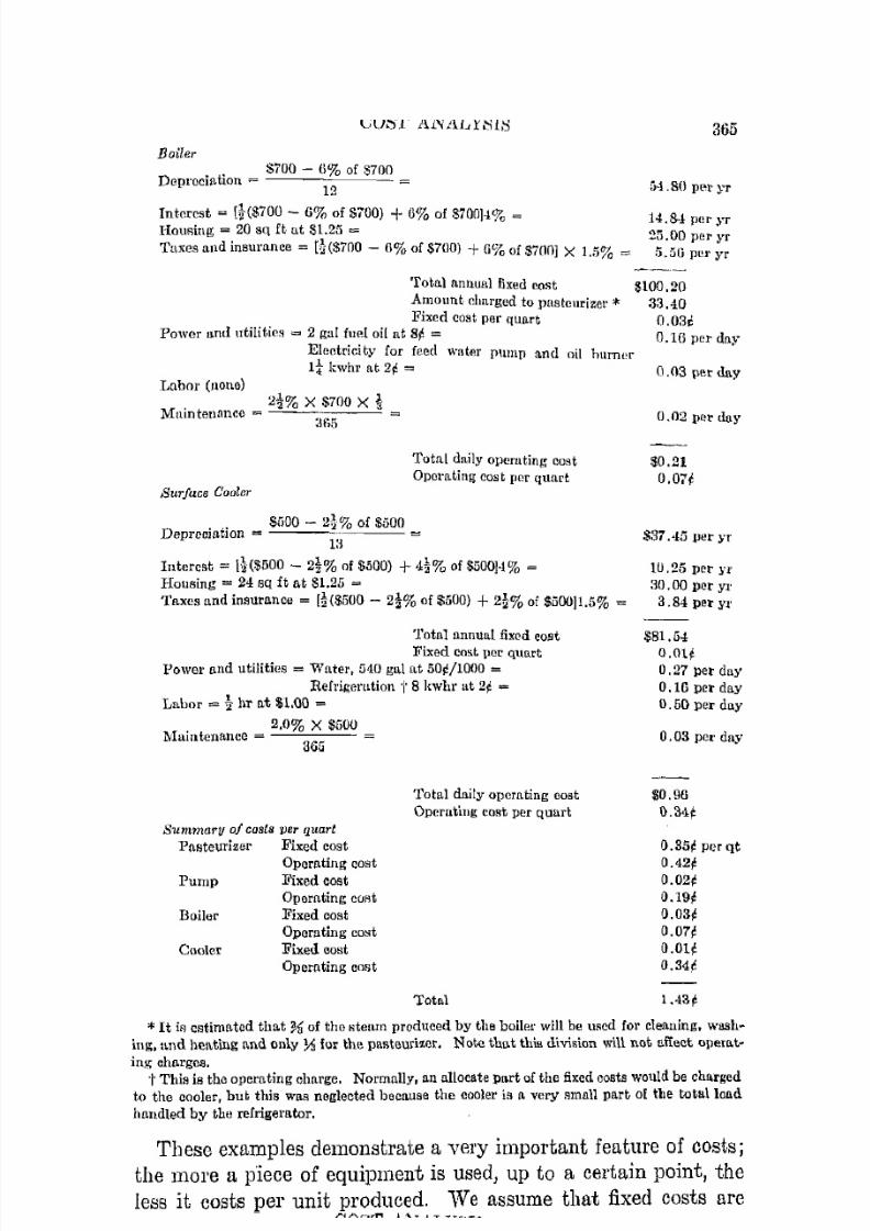
7/16/2019 Engenering Agriculture Perry
http://slidepdf.com/reader/full/engenering-agriculture-perry 385/422
COST ANALYSIS
Boiler. ' 8700 - 6% of 8700
DepreCItLtLOn = 12 =
Interest = [!($700 - G% of $700) + 6% of 8700)4% =
Housing = 20 sq ft at 51.25 =Taxes and insurunce = [ ~ ( 8 7 0 0 - 6% of $7(0) +G% of $700J X 1..5% =
Total antlUal fixed cost
Amount ciHlI'ged to pastenrizer *Fixed cost per quart
Power I1mI utilitio" = 2 gal fuel oil at 8¢ =
Electricity for feed water P\llIlJl and oil hurnerI i kwhr at 2¢ =
Labor (nono)
2!% X 8700 X !Mitintennncc = - - - - - - -
=~ 1 f i f i
Surjuce Gooler
Total dnily operating cast
Operating cast per quart
. , SUOO - 2 ~ % of $500DeprecmtlOn = - - - i : ~ - - - - =
Interest = [}($500 - 2 ~ % of $500) + ~ % of $500J·I% =
Housing = 24 aq ft at 81.25 =
Taxes and Insurance = [!(8500 - 2!% of 8500) + of $500J1.5% =
Total annuul fixed costFixed cost pel' quart
Power and utilities = Water, 5,10 gal at 50t/lOOO =
RefrigenLtion 'I' 8 kwhr at 2¢ =
LILbor = ! hI' at $1.00 =
2.0% X $500rvluiatenll.ncc = =
3G5
Summary oj cosls 'per fluarl
Pasteurizer Fixed east
Operating costPump Fixed cost
Oporating CORt
Boiler Fixed oost
Cooler
Operating cost
Fixed oost
Operating cost
Total daily operating east
Operating l ~ o s t per quart
Tot.l
365
;;·1 .SO per yr
14.84 per y r
25.00 per yr
!) . 50 p l ~ J ' yr
$100.20
33.·10
0.03':
D.W per d"r
0.(13 per day
$0.21
0.07t
$37,015 Jlet yr
lU.25 pet Y1'
30 .00 pet YI'
a 84 pet :1'1'
$81.54O.Ol¢
0.27 per day
O.W pet day
0.50 per day
0.03 pel' day
$0.96
O.34¢
O.35¢ per qt
O.42¢O.02¢
O.19¢
0.03¢
O.07¢
O.Ol¢
O.34¢
1.43¢
* t is estimated that % of the steam produced by the boiler will be used for cleaning, washlng, lLlld hel\ting and only ~ lor the pasteurizer. Note thlJ,t this division will not t!.flect opemt
ing churges.
't This is the operating charge. Normally, an l1110cate part of the fixed costs would be chll.rgedto the cooler, but this was neglected bec!luse the cooler is a very small part of the total load
handled by the refrigerator.
These examples demonstrate a very important feature of costs;the more a piece of equipment is used, up to a certain point, the
less it costs per unit produced. "\Ve assume that fixed costs are

7/16/2019 Engenering Agriculture Perry
http://slidepdf.com/reader/full/engenering-agriculture-perry 386/422
366 AUlUCULTUHAL PROCESS ENGINEERING
not a function of the amount of \lbe. This is essentially true
exeept that a piece of equipmenL may have u shorter life if use(l
extensively. On the other hand, actual life is affected by manyfactors as previously indicated so thai, the acCual weight of tItle
in thiti consilleration is Rmo.ll. Thereforc, the usc, nnit (lORL, annual
fixed-co::;t relationship would hr nearly
Total anllual fixcd co:-;(,Fixed oost per unit = ---------
UniiR produced per year( L4.9)
I t is true that a maehinp that is use(l extpnsively generally
requires greater maintenmw(' cxpom;c P('1' unit as it agcH Ulan one
8
7
6
Vl
1:: 5OJu
: f.c
214"'iiiau
~ 3
2
\\\ ~
400
"-'r -Fixed -r--
c ~ s tI I
I T IOperating
cost
800 1200 1600 2000 2400Bu ground per year
Fig. 14.3. Re1:.ttionshill of tot.al rost per unit, 10 [1mount of usC' per year.
used less. However, power and labor costs are usually much
greater per unit so that any increase in maintenance cost produces
a small if significant increase in the operating cost pel' unit. Con
stant operating costs clln be assumed without seriously affecting
the validity of the results.
7/16/2019 Engenering Agriculture Perry
http://slidepdf.com/reader/full/engenering-agriculture-perry 387/422
COST ANAL1'818 3n;
This relaLiomJlip for the feed grinder is shown in Fig. 14.3.
Irrespective of the nU10unttl of llse the upcrating eoi't, i::; eomtant,
whereas the fixed cost is hyperholi<:.These examples show that labor i8 a hig (··()i"t item. This ie: true
in general. Better woe of labor is wmully the m()st effective way
for lowering operating costs.
14 . 15. Selection, General Principles. The seleetiull of a new
piece of equipment 01' the decision to l'Cphlel' an 0111 pieec of el[uip
lllcnt cannot always be based upon a definite procedure. 1f re
quently, judgment must he relied upon heavily. The proeedure
outlined in this chapter can be usee! fnr close l'stimation ofunit e o s t ~ , hut judgment must be used when such faetul'li a:,; fu
ture prices, consumer demand, and raw-materials supply lllllst be
considered.
REFERENCES
1. Armstrong, C. V. I n d u ~ t r i a l ProperLy R e ( ~ o r d s for Aeconnting and
Valuation Uses. ]0. En(l. E':rpl. Sla. Bll.!l. 160. 19,1<1.
2. Bullinger, C. E. Enuinct'J'ino Economic iinnl};;iis. l ~ I ' I ( J G r [ \ w - H i l l . 1942.
3. Davidson, .T. B. Life, Service and C o ~ t of Service of Farm Mllchinery.la . Au1'. Expt. Bfa. Bull. 260. H129.
4. D[widson, J. B., lind Hendersoll, S. l ~ < i l i l t o l 1 . Life, Sel'\'i(,c [lnd Cost of
Service of Farm Mnehincs a ll 400 Iowa F n l ' l l l ~ . la . A{/I'. KepI. 8[(1.
BlIll. 1'.37. 19,12.
5. Porry, .r. H. C!hclIdcaZ EnGineers lImalbook. Tllinl Erli1ion. McGraw
Hill. 1950.6. Roadhouse, C. L., llnd Henderson, .T. L. 'The M.IlI'/wt J1Ii/l., hl(lzlsirll.
l ~ i r s t Edition. McGraw-Hill. 1941.
7. Winfrey, Robley. Depl'Ccitltion uf Gl'OUp Properties. la . E'n(l. R:rJiI.
Sfa. Bull. 155. 1942.8. Winfrey, Robley. Statistical Analysis of Industrial Property Retire
ments. la . Eno. EJ:pt. Sta. B1l11. 125. 1935.
9. U. S. Trel\slll'Y Department. Incorne Tax Depreciation and Obsolcsecnuc.
Estimated Useful Lives nud Depreciation Rates. U. 8. Bill'. Internal]tcue/ille Bull. F. U. S. Government Pl'inting OftieD.

7/16/2019 Engenering Agriculture Perry
http://slidepdf.com/reader/full/engenering-agriculture-perry 388/422
CHAPTER 15
Process Analysis
and Plant D e s i ~ n
The p<:orfmll_I.'t11lCC of a llrOJcc\'>);ing plant (lellemb upon lhe effi
ciency with whi('h the material flows through the plant. Efficiency
us here used refers to the aecumulated effieiencies in the usc of
individual llIachines, labor, power, utilities, storage and work
Rpace, roac1l, and LranRj1ortation, and athol' facilities noccss[tl'Y
for production.
The various aetivitieJ:l that constitute a process must be so integrated that the movement of material through the plant 11l'OCeeds
smoothly and with a minimum of interruption. I f tho operations
are more or less autol11ittic and control personnel only is required,
tho location of units, conveying systems, and storago areas can be
arranged with officient performance of tho units being the prime
objectivc. I f the activities are mostly manual, the operations
must be set up in light of convcnience, safety, and productivity
of the workers in addit,ion to efficient machine performance. Aprocess must be so constituted that normal eontingencies such as
breakdown, irrregular rate of influx of raw products, and change
in characteristics of rtlW pl'oduets will not disrupt the normal
operations. These factors and others of a flimilar nature must be
C'onsidered when analyzing a processing operation.
A complete processing plant consists of a number of unit opera
tions or processes arranged in a certain sequence which may he
simple, as in feed grinding on the farm, or complex, as in producing cotton-seed oil or soybean oil, for example. In designing
a new plant or rearranging an existing plant for more efficient
operation, certain established procedures should be followed in
oreler to secure the most satisfactory results. Process charts and
368

7/16/2019 Engenering Agriculture Perry
http://slidepdf.com/reader/full/engenering-agriculture-perry 389/422
PROCESS ANALYSIS AND PLANT DESIGN 369
flow diagrams" which will be discussed in this chapter nre excel
lent tools to use for studying an existing processing plant when
improvements arc needed or for (lesigning a new plant.
PROCESS CHARTS
A process chart is a schematic presentation of a p1'O('.8:':8, show
ing the events which constitute the proeess, their order, and cer
tain desired information concerning eueh. Chart forms are varied
since each individual problem is unique. Thc experienced process
analyst is able to tailor the ehart to the situation at hand, but the
novice should follow eertain procedures that are known to be
satisfactory in most studies.
There arc three types of process charts, although it is not always
easy to distinguish between them when in use.
15.1. An Operation Process Chart is a graphie presentatiull
of al l the events in a process ane! their sequence. The time re
quired for each event or operation and the distance between
operations may be included if pertinent. Other information llW.y
be added if it contributes to the study. The operation p r o e e s ~chart is used for studying the entire operation.
15.2. A Flow Process Chart is It graphic prcsent[1tion of all
the operations and al l intermediate events showing transpnrta
tions, inspections, storages, and delays. All i n f o n n l ~ t j o n needed
to meet the analysis objectives is ineluded, for example, labor
required, times, distances, capacities, utilities, temperatures, and
other information. The flow process chart may represent the
entire process, but because of the volume uf detail it is generally
mice! for significant parts of it only.
15.3. The Layout Sheet or Layout Diagram is I t graphical
plot of operation or event locations showing the direction of flow
of materials and labor. I t is usually a plan layout to scale show
ing spaee utilization and direction of movement of materials.
However, elevation anti thrct>-nimensionul presl'ututions are fre
quently used.
*Manual opemtion economy discussed in Chap. Hl, is closdy rclateu to
process efHcieney and should UP. considered when designing a llew plant or
!tnulyzing a going concern.

7/16/2019 Engenering Agriculture Perry
http://slidepdf.com/reader/full/engenering-agriculture-perry 390/422
370 ACRICULTURAL PROCESS ENGINEERING
15.4.. Nomenclature. Studies have shown that a p1'oce::-;::; is
composed of five types of i':ltepR ill various combinations. These
Hteps and Hymbols which have been sirmdal'dize(l hy til(' Anlcl'iean
Hoeiety of Mechanical Eng,ineel'H r follow.
1. Operation O. AllY udi\'ity that altl'rK the jlhy::;ical or
('helllical c:hal'adel'istics of a llIaterial 01' al l objuct, 01 ' nddc; tu
it in any way wlwtsoevC'r, sHeh [ I " grinding grain, dl'ying hay,
wC'ighing C'ggK, freczing lllPaj, llailiug box, Ilwiling ldtc'l'.
2, 'l'rIll18jJ01'iutioll I=? Any 1ll0VC'lllcnt of matt'l'inl i't-om one
place to another unleR" :mel! movelllent is an intt'gnd part uf anoperation, sueh as milk by pump, rC'fUiiC by tmck, fl'uit by belt,
box by elllployee, grain by tl'Urk.
a. Insz)('ct?:on D. An examination by an individual to deter
mine quality 01' quantity or to verify conditions, sueh as de
termining llloisture conkllt uf grain, (iPtcl'lllining g,l'l1llc of fruit,
('hecking porIonnHnce of vegetable washer, notill!!; temperature of
pasteurizer.
4. 8tomge V . A (lcsirable interruption (If acLivity, such asingrcdients being held for future UHC, fruiL being, 11('1(1 for optimum
market.
5. Delau D. An uudcflirahlc interruption of adivity, Huch aH
prullm; in tray vi"aiting to be ,lrieri, marlcrinJ in tl'll!'k \Vltiting to he
unloaderl, employee waiting for machine to operate.
6. Combined Operation. Where two 01' more operationfl take
plaee simultaneously, Lhe requisite Rymbols art' romhinml. :For
example, cheese in a proce::;t-:ing room is both LL i:ltllrngc arl(l LLn
operation; a lllixing pl'oce"s may he both an opcraLion ant1 u
transportation.
Process rharts lllay be built mouud (1) materials, (2) men, o!'
(3) maehines. They may show tlt(, movement of materials and
all operations thereon. They may :-;bow Lb(' aetivitie8 of a man
01' 1llpn required Lo produce a r.crLain enrll1oint. Or the (l,etivitieR
of a machine 01' &eries of machine::; may he represente(l.
15.5. Operation Process Charts. An opel'a.trion }11'OC08::; ellal'\.of seed preparation is shown in Fig. 15.1. It will he nS(,11 to
demonstrate the method::; of chart detlign all(l its use.
Operation process charts can be pl'epared on plaiu sheet:=> of
paper of suffi('icnt size to include al l the required operntiolls, 01' a
form "Heh as "hOWll can be used. The ehart type is mate?1rd, man,
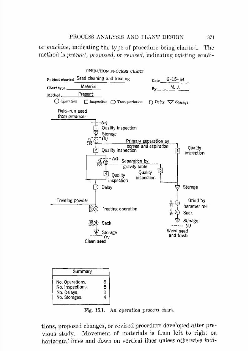
7/16/2019 Engenering Agriculture Perry
http://slidepdf.com/reader/full/engenering-agriculture-perry 391/422
l'RCJCEtiS ANALYSIS },ND PLANT DERlG:\' 371
or macf!7:lle, indicat.ing the type or procedure being charted. The
method is present, proposed, or revised, inrlieating c x i ~ t . i n g cOlldi-
OPERATION PROCESS CHART
Subject charted Seed cleaning and treating
Chart type _ _ ..;.M...;.a:.:te...;.r.:.:ia...;.'_
Method__ - ' P c . . : r . . : : e : : : . : s e : . : . : n ~ t _
Date 6-15-54
By__ .;.;M'-'" .;.J:....._
o Opcmtion 0 Inspection c:> Tmn"portatioll 0 Delay V'" Storage
Field-run seedfrom producer
Treating powder
Treating operation
Storage- - - - - - (e )
Clean seed
Summary
No. Operations, 6No. Inspections, 5No. Delays, 1No. Storages, 4
Qualityinspection
Storage
Grind by
hammer mill
Sack
Storage------ (c)
Weed seedand trash
Fig. 15.1. An opemtioll process chm"l.
tions, proposed changes, or revised procedure developed [lfter pre
vious study. Movement of muterials is from left to right on
horizontal1ines and down on vertical lines unless otherwise incli-

7/16/2019 Engenering Agriculture Perry
http://slidepdf.com/reader/full/engenering-agriculture-perry 392/422
372 AGRICULTURAL l'HOCEAR gN<\lNK1I}RINO
cated by arrows. The main flow should begin at the top of the
Hheet and proceed straight downward. MnLPl'ial added to the
main line of flow is indieatccl by a horizontal line to the left ofthe main-line flow. Matel'inlremovecI is indicated by a horizontal
line to the right of the muin flow line. ConvenLional details fino
their meaning are "hown in Fig. 15.2.
Material added to the mainIme prior to an operation
Material removed as theresult of an operation
Matenal added to the mainflow during an operation
Material divided with nooperation bei ng performed
Optional process routes indicatedFig. 15.2. Conventional ['ollRtrne1ion d e t a i \ ~ used in Pl'eplHing an operat.ion
]JJ'oceHS ehar!.
The fractions a('compunying each operation indicate the actual
mte in bushels per hour over the capaciLy. This is an excel
lent index for continuous-flow p1'ocel:\scs. I f the material being
processed can he segregated into units, n single bir(l in a poultry
processing plant, for example, the time expcn(lc(l on each unit
during each operation is usually used. Time is use(l only if it
contributes to the analysis.
The summary of sLeps may be omitted, but it shows the balance
between the various types of events and usually is an aid to
analyzing a process, especially if it is complicated.
7/16/2019 Engenering Agriculture Perry
http://slidepdf.com/reader/full/engenering-agriculture-perry 393/422
PROCESS ANAL1'818 AND PLANT DESIGN 373
rrhe following should be eonsidered relative to an operation
IJl'ocess chart,
1. What Events Can Be COInbl:ned? Combining steps usually
reduces labor and may reduce othcr costs. For example, the
machine used on operation two might be substituted for tli8
machine of operation one. This woul(l eliminate inspections four
and five and operation two. There ~ w o u l c l be a saying in lahar
and amortization of the machine of operation one.
2. Can Inspections Be Eliminated? Inspections freqnently i n ~dieate lack of rcfincment of an operation or series of operations
which could be eliminated by improving operation design or tech
niques. However, if the raw Jlroduct is variable it may be i n ~advisable to attempt to eliminate inspections. Furthermore, it
may be economically advisable to use inspections in connection
with simple economical operations ruther than more expensive
procedures that do not require inspections.
In our example, inspection one is made to determine the quality
of seed received f1'0111 the l)rodueel' il l order to determine the price
to be paid. The other inspections arc necessary to adjust theoperation of sorters.
3. Can Delays Be Eliminated 01' Converted hila Storages!
D l ~ l a y s and storages are similar exeept [t delay iii undesirable
whereas a storage is desirable, A delay makes it impossible to
usc men or machines in the most efficient way. A storage Illay
fneilitate the use of men and materials.
For example, storage number two retains all the rcject from
operations one and two. When seed is not being delivered from
the producer at the maximum rates, labor can be released fr01l1
the major operations to grind, sack, and store the reject. The
delay is necessary because t h ( ~ treating equipment does not have
sufficient capacity. The Bcparating and sacking capacity i:-; 100
bu PCl' h1', the rate being controlled by operation number two.
The slower treating operation actually reduces the potential ca
pacity by half.
An operation proccss chart is usually prepared as a basis for amore detailed study of parts of the chart which arc known to Ileed
improving. This need may have been recognized before the opera
tion process chart was prepared or may have been discovered
through study of the chart.

7/16/2019 Engenering Agriculture Perry
http://slidepdf.com/reader/full/engenering-agriculture-perry 394/422
374 AGHI< 'ULTUHAL PHOCE:-iR ENc:INKERING
7/16/2019 Engenering Agriculture Perry
http://slidepdf.com/reader/full/engenering-agriculture-perry 395/422
PROCESS ANALYSIS AND PLANT DESIGN 375
Fig. 15.3 is a pictorial operation process chart of English walnut
processing. Charts of this type are more difficult to make than
tho graphic type, but they are hequently used for popular presentation because of clarity. Data can be added so that an analysiscall be made if needed.
15.6. Flow.Process Charts. Fig. 15.4 is a flow process chart
of the portion of the operation process chart in Fig. 15.1 desig
nated as (b), (d), and (8). A detailed study is desired in order
to correct the delay prior to the treating operation.
The flow-process chart form is so set up that columns are pro
vided for most of the information required in any study. The
blank columns can be used as the situation demands, in this caso,
for labor and power.
Relative to the information on the chart, consider the following.
Each individual step is listed even though some steps may be of
minor impOl'tance. The chart symbols and identification marks
are the same as used in the operation process chart.
I f single units arc moved by hand, the distance llloved may be
of significant value because of the labor used. I f movement is bymechanical conveyor, the distance may not materially influence
labor requirement. A "V" following a distance indicates that it
is vertical. The distance index for conveying to delay chamber
indicates a total travel of 25 ft, there being a vertical lift of 10 ft.
The distance moved is horizontal if no identifying index is used.
Ini'ormation concerning the direction and method of movement
may be used for determining materials-handling design data.
The unit times will probably be important i f distinct units ofmaterial 9,re heing processed, animals in an abattoir, small lots
of vegetables in a community canning plant, a kettle of sorghum,
or any batch process, for example. In cases of this kind, the time
of each step is important since the arithmetical total is the total
time required and the breakdown indicates steps that might be
shortened. The unit times for continuous processes such as vege
table washers, seed cleaners, drum dehydrators, and walnut hullers
are not so important. Sinee the events occur simultaneously, laboris uSllfllly not proportional to the individual times and inspec
tions; delays and storages can occur without affecting the normal
flow; the total of the times listed is not usually the total time
required for a complete process. However, the totnl of the unit
operation times and the unit transportation times is the total time

7/16/2019 Engenering Agriculture Perry
http://slidepdf.com/reader/full/engenering-agriculture-perry 396/422
376 AGRICULTURAL l ~ R ( ) ( ~ E S S RNGINEElUNG
required for the actual processing. The individual vnlues arc im
pOl'Lant in determining the time the material is subjectecl to all
FLOW PROCESS CH4RT
Subjeot oharted Seed Cleaning and Treating
Chart begins Material Entering Primary Separator (b)
Chart onds Material in Storage (d- e)
Type of chAlt..::Mc.::a"'ter:.:;ia:.:._I________
A t h rtcd 50 bu/hroUn or Tao c-c a..
P r o c ~ B s Description C}mrt Dial, Unit TilUes in
Shoet _I_of _1_ sheets
Date 7-6-53
Charted by __:M:::_ :_J.:.,____
o p ~ r a t i Q n c::::> Transportation
o Inspecti n 0 Delay 'V Storage
hr Man- . POW-Sym- Mov- ( k ~ k r )f Present Method holll cd Oper. Insp. '!'ran. Delay Slor, hr
Primary separation
CD 0.67 0.1 4.25Inspect for foreign material [JJ 0.02 0.1
C o n ~ e y to gravity table -i . 12' v 0.01
Final separation <1) 0.67 0.2 3.20
Inspect for quality IT! I wk 0.3
Convey to delay chamber + 25'0.01
-0.9010 v
Delay to treat [i ) 0.33
Seed treated ® 1.00 0.2
Convey to sacker + 8' O.oC 0.75
Sacked CD 1.00 0.7Sacks conveyed to storage 1+ 60' O.oC 0.6
Storage for sale W 5 rno
Totals 105' 2.2 9.10
Note: Under I!ansportation, C s by chule, Eby elevator, T by truck, indicates vertical distance.
Fig. 15.4. A flow process chart.
event, whether certain operations are performing at peak capacity,
and, eventually, what can be done to adjnst difficulties due to rate
of movement.
The blank spaces are provided for tabUlating important data
such as labor, utilities, moisture contents, grade factors, tempera-
7/16/2019 Engenering Agriculture Perry
http://slidepdf.com/reader/full/engenering-agriculture-perry 397/422
PROCE::;S ANALYSIS AND PLANT DESIGN 377
tures, space requirements, ane[ other information needed to solvea, specific problem.
Regarding the specific example of Fig. 15.4, the delay is clue to
low capacity of the treater. Note that if the capacity of the
treater were doubled, the delay could be eliminated and the rate
increased to that of the gravity table. . In addition, the ca
pacity of the primary separator and sacker would be increaseci to
more satisfaetory levels. Two-and-two-tenths man-hours of labor
are now required; consequently, three men must be on duty.
Doubling the capacity would not; affect the labor requirement of
any operation except saeking and conveying sacks to storage.
They would increase some but not enough to require more Hum
the three men now on duLy. Consequently, [L second or larger
treater could be used to dOllble the capacity and would eliminate
the delay without inereasing the lahar or power requirement.
15.7. Layout Diagram. The layout or flow diagram is used
to locate or rearrange the processing units and to route the
material through the plant in the most efficient manner.
Before preparing the layout or flow diagraHl, the following
information should be secured.
A. Relative to the entire process, refer to operat.ion and flow
process charts.
1. Rate and characteristics of flow in eaeh line. I f the rate
varies, or if fio\v is intermittent, the maximum and mini
mum rutes, their frequency, duration, and time of occur
rence should be ascertained. This information is neeessaryfor design of storage and holding areas and surge chambers
as well as for determining the optimum size of processing
units.
2. Charaeteristies of structmc and area in which the process
is or is to be carried out.
fl. Service facilities, roads) railroads, their capacity, con
nections, relative location, etc.
b. Available utilities and quantities.c. Orientation and prevailing wind characteristics: opcm
tions should be so orientated that workers will not be
required to face the sun 01' to work in heat, dirt, or odors
foreed upon them by the wind.

7/16/2019 Engenering Agriculture Perry
http://slidepdf.com/reader/full/engenering-agriculture-perry 398/422
378 AGRICULTURAL P H O G F , ~ S ENnINEERING
d. Details of structure and area: a vlan drawing should beprepared showing all the detn,ils important from the
stanrlpoint of the processing operation. This will be used
for the layout diagram. I f available, the plan sheet of
the blueprints can be used admirably.
B. Relat ive to each step listed on the process charts.
1. Capacity of unit: this might be a number of small units
with accumulated capacity.
2. Labor requirement and chm'actcri&i,ics: space needed for
workers, light, etc.
3. Space requirements for unit, service', and labol'.
4. Utilities required: light, heat, refrigendion, power, water,
steam, gas, sewage, ventilation, etc.
5. Materials required for flow in antI out of unit.
A new layout can be prepared or an existing layout can be criti
cized on the basis of the above information. Engineering judg
ment must be exercised in this sLep since no two plants are the
same. However, the following suggestions, which are based upona discussion of plant layout practices by Maynard and Stege
merten 1, will be of measurable assistance in most layout jobs.
15.S. Layout Procedures. Many plants luwe been and some
still are laid out on the basis of the following principles.
1. The raw product should come in at one end of the plant and
should emerge in the finished state at the other end.
2. Aisles should be provided for transportation purposes andshould be kept clear at all times.
3. Like operations should be grouped and arranged in straight
lines or orderly rows.
4. Ample space for placing material should be provided around
each operation.
Layouts prepared on the basis of these principles were pleasing
in appearance, and orderliness and lack of crowding resulted.
However, after making a number of detailed studies of this type
of setup, many inefficiencies were found to exist. Material and
employees had to travel too far. Materials-handling labor was
high, it was frequently difficult to provide an efficient {low pattern
for the material, and there was too much waste space. This
7/16/2019 Engenering Agriculture Perry
http://slidepdf.com/reader/full/engenering-agriculture-perry 399/422
PROCESS ANALYSIS AND PLANT DESIGN 379
realization and careful studies produced a ne\v set of principleswhich are:
1. The material from one operation should be placed in such aposition that it call be most easily pieked up for the next opera tion.
2. The distance l l l l operator must move to obtain or delivermaterial mvay from a machine should be reduced to [ t minimum.
3. Time spent by [ t machine performing an op(;ratioll or part
of an operation whieh does not require the immediate attentiollof the operator or aLtcndant is idle time as far as the attendant
or operator is concerned.
Plants laid out on these three principles are very efficient,
although the arrangement may appeal' chaotic to the uninformed.
The layout can be mos!; efficiently studied by using a floor planof the area to he utilized nnd tmnplets of the erlllipment to be
located or rearranged. The temp lets should represent the e q u i p ~ment to scale and can be cut out of heavy paper, cardboard, p l y ~wood, or any suitable material. T h r e e ~ c l i l l 1 e n s i o l l a l templcts may
be advisable if height is a factor. T h r e e ~ c l i l l 1 e n s i o n a l te1l1pletscan be made of heavy paper, cardbourd, or cut from wood blocks.
The templets can be shifted to various locations, and studied andcriticized until thc most satisfactory arrangement is found. The
templet::; can be fustened with tlmmhtacks, map tacks, rubber
cement, staples or any other suitable fastening. String, perhapscolored, ca.n be used to show the direction of flow.
REFERENCES
1. A.S.M.E. Operation and Flow Process C!wris. American SocieLy Me-
chanical Engineers. 1947.
2. Barnes, R. M. Motion and Time Study. Wiley. Third Edition. 1949.
3. Bames, R. M. Works Methods Manual. Wiley. 1944.
4. Maynard, H. 1-1., and Stegerncrten, G. J. Operation Analysis. McGmw
Hill. 1939.5. Munclel, M. E. Syste;nati(;.M otion and ,['ime St1ldy. Prentice-Hall.
1947.

7/16/2019 Engenering Agriculture Perry
http://slidepdf.com/reader/full/engenering-agriculture-perry 400/422
C H A P T E R 16
MmuwJ Operation Economy
Proccssing opcrations are automatic, semiautomatic, or manual.
Automatic opcrations do not requirc contimloutl attendancc, forexample, refrigeration, drying h[\y with forced air, separat,ion ofcream, etc. Operations that require continuous attendance of an
operator whose main function il:l supervision or control would be
considered semiautomatic, for example, evaporating cane syrup
to mobsses, opentting a holding pasteurizm', rendering lard, etc.
Processing farm products includes many operations that arc adirect function of manual activity, such as candling eggs, grading
fmit, dressing poultry, feeding a hemp mill, and packing freshvegetables for shipment.
The cost of a manual operation is directly proportional to the
time required to do it. A competent worker is capable of a defi
nite amount of manual output per day under good conditions.His surroundings shoulcl be so managed and arranged that the
maximum amount of his available energy will be expended use
fully. Management must cooperate in the following respects in
oreler to insure itself economy in manual operation.
1. In order that labor may h a v ~ the desire to produce, mftll:1ge
ment must provide the following:
a. Satisfactory working conditionH: good light, proper tem
perature, clean surroundings, good servic:e farilitieR.
b. Proper personnel relationships and techniques: Forell1en and
supervisors must know and use proper managerial methods;
work and rest periods must be properly balanced.2. Equipment layout must pel'lnit labor to pToducc at maximum
rate with minimum effort.
Point a uncler number one was discussed indirectly in Chap. 14.
Point b is beyond the scope of this book, but the student must
380

7/16/2019 Engenering Agriculture Perry
http://slidepdf.com/reader/full/engenering-agriculture-perry 401/422
MANUAL OPEHATION ECONOMY 381
r c a l i ~ e its importance and become vCl'l"cd in the implied principles.
Point two will be discussed hriefly, although it will be impossible
to treat it in as comprehensive n manner as the subjeet needs.l\Totioll and time study is a distinct field that is too involved
and sllecializecl to be treated \\ompletely in this short ehapter.
The discussion that follows will help solve many of the simpler
problems that reSlllt bceause of improper usc or Illation hy labor,
but major problems should be handled by experienced motion and
time-study men or on the basis of material from the referencesat the end of this chapter.
16.1. Definition of Motion and Time Study. Bnl'lles 1 hasdefined motion and time study thus:
"Motion and time study is the analysis of the methods, of the
materials, and of the tools and equipment used, or to he llsed, in
the performance of a piece of wmk-un t1lltlJysis eunied on with
the purpose of (1) finding the most economical W[,y of doing this
work; (2) standardizing the methods, lllaterials, tools, and equip
ment; (3) accurately determining the time required by a quali
fied person working at [\ normal pace to do the task; and ( ~ 1 ) assisting in training the worker in the new method."
The four parts of the field are distinct divisions uf study, but the
solution of any specific problem emmot he made un any single
one. They must be usee! in combination,
16.2. Wol"li. Economy Principles. Barnes 1 has listed ten
principles of motion economy which, when folluwed, permit the
worker to do a maximum amount of work with a minimum of
effort. These principles follow.1. j\I[otions of the two hands Sh01LLrl be s'ilnultancotlS and 8l1rn
met,tical.
Unless special t.hought and study have been given a manual job,
most jobs will be performed in some manner such as this. The
left hand will piek up a part and hold it while the right hand
performs some job upon it. After finishing the work, the left
hand rejects the finished job and the process is repeated. Ac
tually, the left hand assists the right hand and the rate of produetion is a function of the right hanel's activity. I f both hands
are trained and permitted to perform simu1taneously, the rate of
production will be increased without increasing the physical out
put of the operator.

7/16/2019 Engenering Agriculture Perry
http://slidepdf.com/reader/full/engenering-agriculture-perry 402/422
382 AGRICULTURAL PROCESS ENGINEERING
This principle is particularly rehtecl to fruit and wgetable
picking operations. Two-handed symmetrical production is ap
proximately 20 per cent faster than one-handed operations inwhich one hand assists the other.
The pin board of Fig. 16.1 can bc used to demonstrate the im
portance of this principle. TIle pins are placed in front of the
[ )
@@@@@@@@@@@@@@@
@@@@@@@@©@@@@@@
Fig. 16.1. Pin board for work economy Rtudy. The board is 7 in. by 8 in.
with % in. holes 1 in. on center and countersunk to % in. diameter. Pinsare % in. by 3 in. long.
board in a random pile. The time required to .Em the board isnoted for the one-handed procedure, that is, one hand passing the
pins to the other hand 'which places them curved end down in the
board. The time is then observed for two-handed simultaneous
independent movements. Bames has found the average times to
be 38 and 23 sec respectively.2. Tools and materials should be located close in and d ~ ' r e c t l y
in front of the o p e ~ ' a t o r so as to be within easy reach of the hands.Transport distances shourd be as short as possibre and movementsshould be as few as possible.
7/16/2019 Engenering Agriculture Perry
http://slidepdf.com/reader/full/engenering-agriculture-perry 403/422
MANUAL OPERATION ECONmvIY 383
The working space of an operator is that defined by his hands
when his extended arms are moved in three planes without mov
ing his shoulders. The best space is that directly in front of theuperator and which is described by both hU11(1:;;.
This prinr.iple can be demonstrated by the pin board. Separate
the board into two parts as shown and move them 12 in. apart.
Observe the time for a simultaneous two-handed fill. Repeat with
a 24-in. spacing. Average times will be approximately 2(1 and 30
sec as against 23 sec for the time with blocks adjacent.
3. There should be Il. rlefi:nite (tnd fi;rerl place for c& tools and
materials.The reason for this is evident. Automatic, fast production
movements cannot he developed if the operator has to search with
his eyes and perhaps hands before making a productive motion.
4. The material shou}d be delivered close to the 'point of USB by
conveyors or gravity.
The material should be placed within the space indicated under
principle 2. The location of the material should not move. The
operator shoulclnol be required to usc his eyes to guide his hrLndswhen reaching for material. The rotating lemon pin of Fig. lfi.2
has a movable spring-supported bottom which maintains the
lemons at a constant level as regards the operator. This facili
tates reaching for fruit that is to be packed which in turn permits
a higher rate of packing than ,,,ould be possible if the lemon level
varied.5. Tools and materials should be p 1 " e ~ p o s i t i o n e d VJherever
possible.Materials, tools, and equipment should be so positioned that a
minimum of physical movement is required to perform an opera
tion. The butcher shop with the saws and cleavers hanging above
the meat block and knives sheathed to the block all within easy
reach of the butcher is a good example of this principle of opera
tion. The handles of all the tools are in such a position that the
hand does not have to move far or the wrist twist much to grasp
H tool.6. "Drop del-iveri.es" shouLd be 1lsed VJherever possible.
Essentially, drop delivery implies that upon completion of an
operation, the product is released and drops into a box, chute, or
conveyor. This type of delivery is very economical of time, arm

7/16/2019 Engenering Agriculture Perry
http://slidepdf.com/reader/full/engenering-agriculture-perry 404/422
38'1 AGlUCULTUHAL PROCESS ENGINEERING
movement, and energy. Fig. 16.3 is a drop delivery for reject
lemons. Note the r:,horL distance and small amount of lifting
required to complete an operatlOn. This contributes to bothefficiency and bpeed.
7. The hands should be Telievecl of all work that can be done
/;y the feet, lJOwel'-opemterJ tools, and Jigs and jiXhl1·BS.
FIg 162 The lemon park-oul bin has [l. spring-supported bottom, which
m:untains the top positIon a1 the same elevation irroo.pedive of tho quan
tIty In the bin. The bill rotates slowly, tllf'l'cfore filling is unifollii(Courtesy Food Machinel}' Cmp)
The trash can with a fooL-operated lid minimizes the til1le and
energy required to dispo:;e of t1. quantity of refuse. In a feec!
mixing plant an electric sark :-,ewer which is moved across Lhe
sack by hanel i::; fa:;ter nnd less tIring chan doing the job by hand
with a hand shuUle.
8. Materials and eqllipment should be located to permit thebest sequence of motions. Rhythm is essentiaL to a smooth ensy
work pattern.
Rhythm illll)lics that motions in a productive sequence occur
systematically without distinct ureaks or abrupt changes and

7/16/2019 Engenering Agriculture Perry
http://slidepdf.com/reader/full/engenering-agriculture-perry 405/422
MANUAL OPERATION ECONOMY 385
proceed with a characteristic swing. Circus roustabouts driving
tent stakes, an experienced farmer shoveling grain, an expcrienced
egg candler are examp1es of the type of rhythm desired.
Fig. 16.3. Sorting effort is reuuced when urops are used to receive ther ! ~ j e e t 8 . Note the short disLlLllce the hand must move to reject an unde
sil'abh-! fruit. (Courtesy Food Machinery Corp.)
9. Smooth continuous molcions of the hands acre 1)referable to
zigzag motions 01' straight-line mot7:ons involving S1idden andsharp changes in direction.
This principle is direct1y related to principle eight. Studies
have shown tlfat in such a simple operation as moving a pencil
Lack and forth across a sheet of paper, that 15 to 25 per cent of
7/16/2019 Engenering Agriculture Perry
http://slidepdf.com/reader/full/engenering-agriculture-perry 406/422
386 AGRICULTURAL PROCESS ENGINEERING
the time is consumed in changing direction of motion of the hand.
Comparable inefficiencies exist on processing operatiollS that rc
qnire zigzag or jerky movements.10. The height of the work place and the chair shonlcl prefer
abLy be an-anged to perrnit olterna[e sitting and standing at
11'01"". Adeq'Uftie lighting Rhoulcl be provided, and the 'Worker
sho1l/rlb!' made as com! ortahle as poss1:ble.
MUHt work pORitiom; can 1)(' rlrsigncd RO Chat the operator call
bit or stand as rlcRircd. This f'ontriblltes to effiriency. Lighting
and other surrounding conditiom, lllust ('onfol'll1 to rccoguized
industrial standards.16.3. Standardization. A ftc!' Illethods have bet'll developed
whieh mort a speeifi(: objcC'tivc, management must (l) provide
facilities, (2) trtLin the workertl in the accepted procedures, (3) in
sure llmintentLnre of the standard, and (4) do these things in the
eaRiest and most economical manner.
SttLnclurdized methods involve machines, men, materitLI::l, and
surroundings. A record shonld be made indicating all the dettLils
that are necessary to carry out the tLcccpted procedure. Thisrecord should indicate the design of the machines, their operating
characteristics, the speeificatiolls of mtLtel'ials, and working eOll
ditions. A procc(lure should he developed for ch('C'king t1llfll11ain
taining these conditions since machines will get out of adjustment"
the characteristic of raw materials will VtLl'y from lot to lot, and
worki.ng conditions rimy chrmge with time.
M[tchi.nes and equipment should be standanlized as much as
possible so that conversion, rearrangement, or change CtLl1 be madewith tL minimum of time, labor, and expense. Management must
recognize and foresee the possibility of variMion in production
and proville for it. For eXtLll1ple, box-making machines should be
flexible enough so that they can be changed to make boxetl of a
di.fferent size if needed. Benches and conveyors shOUld be s t a n t l ~ardized so they can be tLrrangefl with a minimum of altemtion to
handle a diffcrent material if materitLl vnriation is expected.
16.4 . Time Study. Time study is the procedure used to e v a l ~uate a manual operation or series of unifieclmanual operations in
order to provide procedures facilitating the greatest output with
average normal worker effort. Three steps are involved in the'
procedure; these are:

7/16/2019 Engenering Agriculture Perry
http://slidepdf.com/reader/full/engenering-agriculture-perry 407/422
MAt\UAL OPBRATION ECONOMY 387
1. Dete1'l1!1·ne the capacity 01' nOl')1wL or standard olitpnt of the10 O1'Ice?'.
In some cases this ean be determined by analyzing the movements of the most productive worker in a group and then udng
this amLlysis as a basis for recommendations. Or it may be necessary to analyze and improve the current ineffwient procedure tosecure a suitable standard,
The standard or basic output 01' capacity should be based uponthe most efficient use of effort possible and should be at suell a
speed that maximum production can be realized without fatigne
to the operator. The standard or minimum wage is usually basedupon the standard production rate with incentive piece-work rateR
for production over and above the standard. This makes it possible for the worker of average energy to do an acceptable amountof work without undue fatigue anel receive a satisfactory wagefor it. The faster or more energetic worker, at the same time,
will be rewarded for his extra production.2. Analyze the present steps in the operation to diminate u,se
less movements and imp1'Ove necessary movement8.Frank B. Gilbreth found that there were 18 elementaJ events
used in manual operations. These events or activities, called"therbligs" (Gilbreth spelled backwards), in various combina
tions compose any and all manual operations or movements,
drinking coffee, sharpening a pencil, wrapping a package, pickinga chicken, picking apples, to cite a few. The 18 therbligs are
listed in Table 16.1.
After dividing an operation into the thel'bligs or other significant events that compose it, the objeetive is to eliminate the
unnecessary therbligs, combine as many of the necessary therbligsas possible, and then rearrange the remaining therblig" or events
in the most satisfactory sequence.
After making the obvious adjustments, the operation is broken
tlown into suitable elements and the clements (which may lIe
composed of more than one therblig) studied on the basis ofrequisite time as taken with lL stop watch. Ree-ent developments
in time study with a motion picture camera, called "micromotion"stUdies, have made possible detailed studies of intricate opera
tions that could not be analyzed by the stop-watch method. Detailed procedures to use will be omitted since they are a separate
study in themselves,

7/16/2019 Engenering Agriculture Perry
http://slidepdf.com/reader/full/engenering-agriculture-perry 408/422
388 ACiH lCULTURAL P R O C F , ~ R l'}NGINF,F,RING
No.1
234.[)
(i
78H
10111213
14-
151617
18
TaNe 16.1 BARIC THERBLIG:-l
SClLn:hFindSelectGrasp
'Therblig
Tl'ansporL lnac lec Il)ositionAssembleUReDisassemble
InspectPl'e-posi iOllRelease loadTrlLl1SpOl't emptyRest for overcoming fat,igllcUmLVoidtLhle clehyA voichble delayPlan
Hold
Explanation, Suggested hll] ~ y e moving as if searchingEye straight as if fixed on ohjectReaching for objed
Hand open fOT grasping objel'tA hand with something in itOhjeet, being placed by hamlTwo or more things put togctherA manipUlation, e.g., tmBing screw()ue part of an assembly removed
Ohserve, e.g., check for colorPlacing nail for drivingDropping content out of hand
An empty hand movingMan seated rcstingParts supply exhaW':te([Operators visitingThought process necessllry before operationRetaining objeet in hann
16.5. Training the Workers. After an improved procedurc
has been developed, it must be taught to the operators. This can
be done by before-and-after moving pictl1l'es, operation charts,
diagrams, or demonstrations.
Many industrial plants give all new employees and apprentices
instruction in mot.ion economy which includes the work previously
discussed plus other information which will help them do their
tasks in the easiest and most efficient manner. This training alsoplaces them in an excellent posit.ion to accept and use new and
improved procedures.
R E I ~ E R E N C E S1. Barnes, R. M. J1I/ot1:on and Time Study. Wiley. Third Edition. 1949.2. Barnes, R. M. Work Methods Manual. Wiley. 1944.
3. Holmes, W. G. Applied Time (lnd Motion Study. Ronald. New York,1945.
4. Maynard, H. B., and Stegcmel'ten, G. J. Operation Analysis. McGrawHill. 1939.
5. Mundel, M. E. Systematic M ation and 'l'ime Sl1!dll. Prentice-Hall.1947.
6. Vaughan, L. M., and Hal'din, L. S. Farm WOl'k Simplification. Wiley.1949.

7/16/2019 Engenering Agriculture Perry
http://slidepdf.com/reader/full/engenering-agriculture-perry 409/422
Allpendix i\
HOME CONVEHSION FACTORS
Multiply
British thermal uni tsBritish thermul units
British thermal unitsBushelsCuhic feet
Feet of water
Horsepower
Horsepower
Horsepower
Horsepower (boiler)
Horsepower-hours
Inches of water
Inches of wuterInches of waterInches of waterKilowatt-hoursPounds
Pounds
By
778.33.9:31 X 10-1
2 . 9 ~ ~ 0 X 10-4
1.244
7.4810.434
42.40sa,ooo
745.7
33,475
2,54t10.00246
(lO.l)
0.0786O.03fi13
8,418
7,000453.6
389
To Obtain
Foot-poundsHorsepower-hours
K i l o w ~ l t t - h o \ 1 r sCubic feet
GallonsPounds per square inch
British thermal units per minuteFoot-pounels per minuteWatts
British thcrmnl units por hour
British thermnl unitsAtmosphere
Feet of airInches of mercury
Pounds per square inehBritish thermalllnits
GrainsGrams

7/16/2019 Engenering Agriculture Perry
http://slidepdf.com/reader/full/engenering-agriculture-perry 410/422
BULK DENSI'l'mS *(From Agricultural 8tatistic8, U. R. D e p ~ l l t ! l l e u t of Agriculture, H).52)
Material
A.lfalb seerlApplesBarleyBeansBluegrass seed
Castor beansCorn, car
Corn, shelledGrain sorghums
Rice, roughRyeSoybeans
Sweet potatoesWalnutsWheat
Lb per cuft
-18.0:38.4:18.4..J.8.0
11.2-2'1.0
:3G.8
28.0 i"44.8
44.8 a,nd 40.0
3G.044.848.044.0
40.0
48.0
*As processed for commercial channels, grains at apprm..imately 14 percent moisture content (wet basis).
'I' Two cubic feet of ear corn will proc\ucE' approximately 1 eu f t of
shelled corn.
390
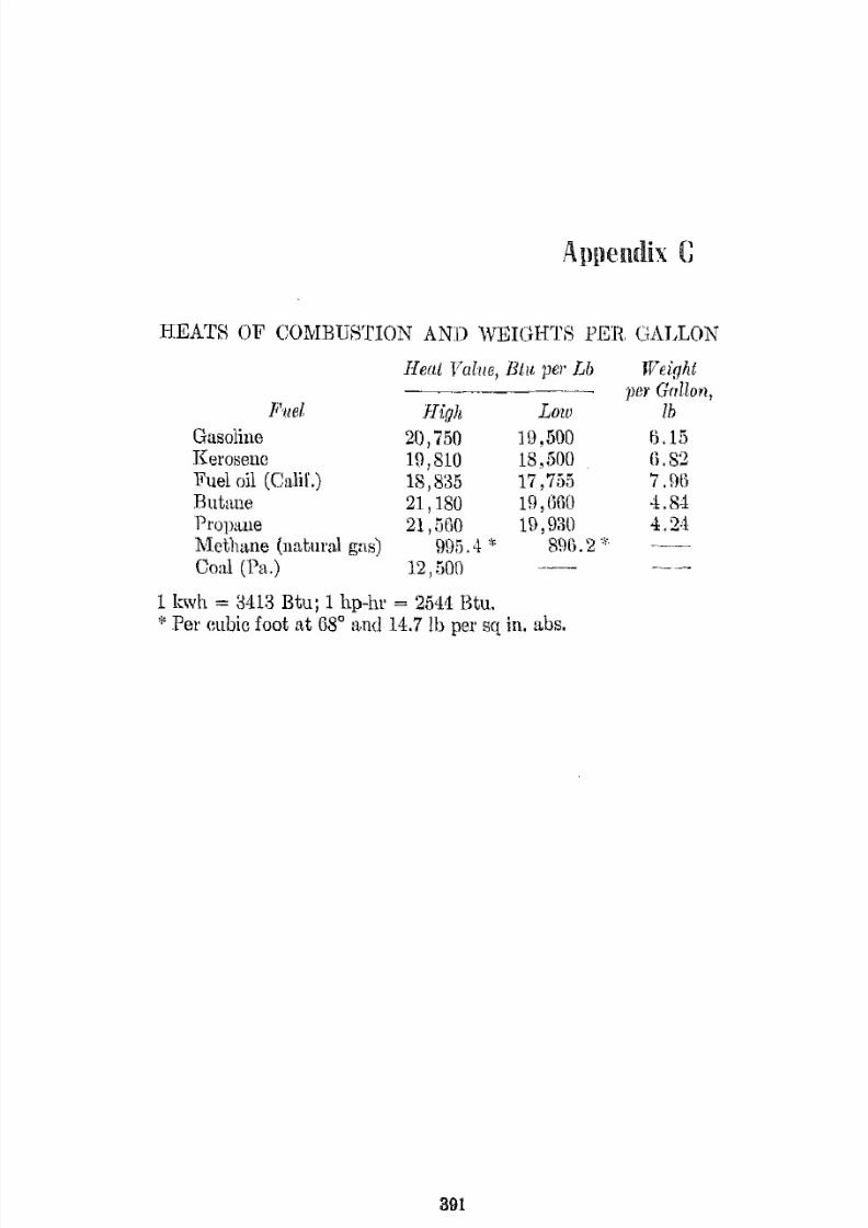
7/16/2019 Engenering Agriculture Perry
http://slidepdf.com/reader/full/engenering-agriculture-perry 411/422
Al1pemHx C
HEATH OF COMBUSTION AND WEIGHTS PER GALLON
GasolineKeroBelle
]i''IIel
Fuel oil (Calif.)
ButanePrOpltlle
Metllane (natural gas)Coal (Pa.)
Heat Value, Btu pet Lb
High
20,750Hl,81018,83521,18021,500
\)95.4
12,500
Low
11),50018,50017,75519,fifiO
19,9303!ll)' 2 *
1 kwh = 3413 Btu; 1 hp-hl' = 2544 Btu.* Pel' cubic foot at 58° and 14.71b pel' sq in. ~ t b s .
891
Weight]leI' Gallon,
Ib
6.15G.S27.nt)4.844.2:1
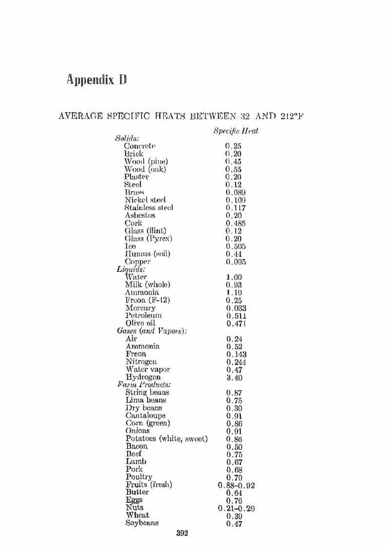
7/16/2019 Engenering Agriculture Perry
http://slidepdf.com/reader/full/engenering-agriculture-perry 412/422
AVERAOE HPECH'fC HEATH BETWEEN AND 212°]<,
Solids:COIH'rot ('
BrickWood (pine)Wood (oak)Plast('l'Steel
B r n ~ ~Nkkc'l steelR t l ~ i l l l e s s steelAsbesj,osCorkGlass (flint)Glass (Pyrex)IcoIIurnllH (Hoil)Copper
Liquids:WHtC'l'
Milk (whole)AmmoniaFreGIl (F-12)MorcllryPetroleumOlive oil
Gases (anri VC!POI'S):Ail'AmmoniaFreonNitrogenWater vaporHydrogen
Farm Products:String beansLima b e a n ~Dry beansCantaloupeCorn (gl'een)OnionsPotatoes (white, sweet)BaconBeefLambPork
PoultryFruits (fresh)ButterEggsNutsWheatSoybeans
392
Sppcijic Heal
0.21'i0.20flA50,5,)0,20(),12
0,089O.lOn0.1170,200,4850,120,200,5050.4<1O,OO!)
1,00
0,031,100,25(j,0330.5110.471
0.240.520,1430,24'10,473,40
0,870.7fi0.300.(110,860,910,8(j0,500.750,670.68
0.700,88-0,920,640,76
0,21-0,290,300,47

7/16/2019 Engenering Agriculture Perry
http://slidepdf.com/reader/full/engenering-agriculture-perry 413/422
SOME PIPE AND TUBING DIl\1ENSIUN:-i
S'l'ANDAUD COf'PBH
S'l'ANDAHD IUON AND S'l'WffiL 1'1PM * TllTlINC; 'i"
Nominnl Actual illJlJ1'oxi1lla/c 81:ze) WaI!8'izc, OD, ID, OD, I'll ckll eS8,
in, vn. In , w. w,I
0.405 0.2i
1
(),0:1Os- -Il'.1 O.MO O.3(i :I 0.030TW0.675 o 4[) 1. 0.030ii' 1
1 0.840 0.62 iJ 0.032' nr1.050 0.82 :1 (I.m2;r 'i f
1 1.315 1.05 1 0.0:3211. .1.1360 1.38 s O . o a . ~4 H
11 1.900 1.61 :1 0.0:']5,"
2 2.375 2.0722
2 2.875 2.47
3 3.500 3.07
S1:ze, Wall Thickness
OD, Range,1/11. in.
-} 0.004-0.04!J
t 0.004-0.0Sa3 0.005-0.13'11i'
! 0.009-0.165:1 0.014-0.238I I
1 0.018-0.31:5
It 0.022-0.313
It 0.025-0.375pT 0.028-0.500
2 0.032-0.625
2t 0.035-0.750
3 0.035-1.000
*Extri1 strengbh pipe with the same OD but with l'mlueed ID is available in 11 number of ranges.
t Various wall thicknesses, the OD remaining constant, [Ire available.Tube types K, L, M for compression and soldered fittingR are t in. largerin OD than the standard tubing (e.g. a t in. type I{ would he il- in. in OD).
t Stainless-steel pipe of the same dimension I'S iron pipe is available.393
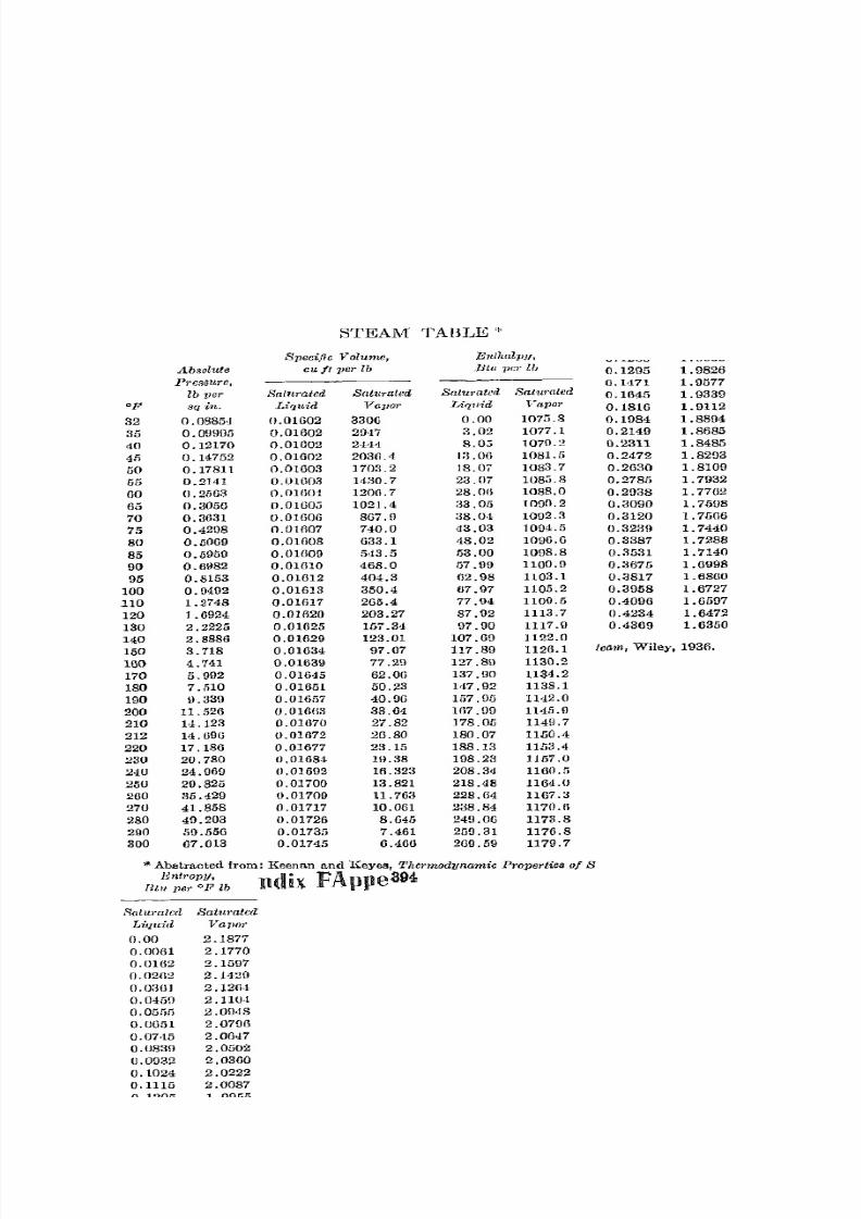
7/16/2019 Engenering Agriculture Perry
http://slidepdf.com/reader/full/engenering-agriculture-perry 414/422
A.ppemlix F
STEAM TABLE *
Specific Volumc, Enthalpy. ]!Jni1'oPY,
Ab.qoZule cu fl1}er lb lJlu pcr llJ UlIJ lUl1' of lb
Pressure,
lb !ler Sai1trated Sal"raled Sa/uratell SaturatedSotiwalcrl 8at'nratclZ
op sq in. L£f]lL't'd lfa1JO )' Liqllid TM101- Li(Juill VallOt
32 0.0885,1 n.01G02 330fj n.oo 1075.8 0.00 2.1877
35 0.09995 0.01602 2!H7 3.02 1077.1 0.0061 2.1770
40 0.12170 0.01002 2-1<11 8.0J 1070.2 0.0162 2.1597
45 0.14752 0.01602 203f1.4 13.0G 1081.5 0.02fl2 2.1420
50 0.17811 0.01603 )703.2 18.0, 10S3.7 O.Oa01 2.12fl.1
(i,5 0.2141 O.()16m 1'130.7 23.07 1083.8 0.0450 2. 110·!
00 0.2563 0.rHOO1 1200.7 28.0(; )088.0 O,05!i1) 2.09,18
65 0.30W 0.0160:; 1021.4 33.05 1090.2 0.0(5) 2.0796
70 0.3631 0.01606 867.9 :18.0·1 1092.3 0.07-15 2.00.17
75 0.4298 0.Olfl07 740.0 ·13.03 1004.5 0.0839 2.0502
80 0.50690.01608 G33.1 48.02 1096.6 0.0932 2.0360
85 0.5959 0.01609 6<13.5 .'i3.00 1098.8 0.1024 2.0222
90 0.6982 O.OlOlO 468.0 57.99 1100.9 0.1115 2.0087
95 0.8153 0.01612 404.3 li2.9S 1103.1 0.1205 1. 9955
100 0.9492 0.01613 350.4 67.97 1105.2 0.1295 1.9826
110 1.2748 0.01617 265.4 77.94 1100.5 0.1<171 1.9577
120 1.0924 0.01620 203.27 87.92 1113.7 0.1545 1.9339
130 2.2225 0.01025 ID7.3'i 97.90 11)7.9 0.1816 1.9112
140 2.8886 0.01629 123.01 107.69 )122.0 0.1984 1.8894
150 3.718 0.01634 97.07 117.89 1126.1 0.2149 1.8685
160 4.7011 0.01639 77.29 127.89 1130.2 0.2311 1.8485
170 5.992 0.0)645 62.00 137.90 1134.2 0.2472 1.8293
180 7.510 0.01051 50.23 147.92 1138.1 0.2630 1.8109
190 \).339 0.01657 40.90 157.05 11<12.0 0.278" 1.7932
200 11.526 o.OJ6m 33.64 Hi7 . \)9 )145.9 O.2()38 1.7762
210 14.123 0.01070 27.82 178.05 1149.7 0.3090 1.7598
212 14. GOG 0.01672 20.80 180.07 1150.4 0.3120 1.71306
220 17.186 0.01677 23.15 188.13 1l5:1.4 0.3239 1.7'140
230 20.780 0.0168·1, l!1.38 198.23 1157.0 0.3387 1.7288
240 24.969 0.01692 HI. 323 208.34 1160.5 0.3531 1.7140
250 29.825 0.01700 13.821 218.48 1164.0 0.367(, 1.6998
200 35.429 0.01709 11.763 228.fl4 11137.3 0.3817 1.6800
270 41. 858 0.01717 10.061 238.84 1170.6 0.3958 1.6727
280 49.203 0.01725 8.045 249.0G 1173.8 0.4096 1.6S!!7
290 59.556 0.01735 7.461 2a9.31 1176.8 0.4234 1.6472
30067.013
0.017456..166 200.59 1179.7 0.4369 1.6350
'" Abstracted from: Keen"n and Keyes, Thermodynamic Properti . of Steam, Wiley. 1936.
394

7/16/2019 Engenering Agriculture Perry
http://slidepdf.com/reader/full/engenering-agriculture-perry 415/422
Absolutfl humidity, 257
Absorptivity, 237
Absorptivity values, 2:17
Accumulator, refrigP.l'ation, 315
Adiabatic process, air-watm'-v:ljJormixture, 261
Aerodynamics of small p a r t . i e l f ~ s , 155
application of, 159
Agrieultuml products, pressure drop
through, 28, 30
Ail' conditioning, process on psychrometric chart, 269
Air flow, branehillg system, design
of, 32
Air horsepower, 114Air lift, 84
Air-operated controls, 349
Air velocities for pneumatic con
veying,204
Amagat's Inw, 256
Ammonia, saturated properties of,
table, 309
Anemometer, hot-wire, 61
characteristics of, 63
rotating-vane, 59
thermocouple, 64
eharaderistics of, M
Angle of repose, 35
Apron conveyors, 189
Aspirating, 15H
Atmosphere, compositioll of, 255
Attrition mills, 132
Batch or bin driers, 290Belt conveyors, belt-loau cross-sec
tion areas and maximulll belt
speeds, table, 183
design of, 182
details of, 180
Index
Belt convevors, characteristics of 1ill)
h O l ' s e p o , ~ e r for, 184 '
Bemoulli equation, 14
Bimotallie t h ( ~ r l l 1 o J l 1 e t e r s , 331
Bill driers, 290Bourdon tube, 48
Brown-Dnvel l1loist,ure t c ~ l e r , 277
Brnsh washers, product, 148
Blleket elevators, U)6
bucket llesign, 200
uischarge from, 197
horsepower of, 200
method of pick up, 199
Bulk densities, table, 390Bnrr mills, 131
characteristics of, 132
By-pass factor, 245
Capillnry tubes, refrigeration, 317
Centrifugal c o m p r e ~ s o r s , refrigera-
Lion, 312
Centrifugal separation, 168
Crntrifuge, 169
Chain, conveying, 186Chain conveyors, classification of,
185
design of, 189
flight speeus of, 189
-llOr"epower of, 190
Cleaning products, 145
COl'fficient of performance, heat
pump, 325
395
rdrigeration, 306CO(lfficienls of friction, v a r i o u ~ ,table, 190
grains, tabll" 36
Coefficients of surface-conductance,
table, 213

7/16/2019 Engenering Agriculture Perry
http://slidepdf.com/reader/full/engenering-agriculture-perry 416/422
396 INDEX
Coefficients of thermal contine! iv-
ity, 212
Column drieJfl, 292
C o m p r e s ~ o r s , rl'friguration, :n 1
Concentrators, 299
C O l l d c n ~ P r s , refngcl atioll, 313
Continuous gravIty-flow driers, 201
COlliroll('rs, llil'-opl'I'a! I'd, :149
no:l[ ing, 847
on-off, 346
"plf-opera! ilH!;, :348
C(lllY(,l'sioll faf'rO! s, tahIr', ClFm
Cost analy",is, 31)2
CORt fl, fixe( I, 35:3
operat ing, 31)3
CL'aue", 206
C['('am separator, 170
Crushers, 132
Cydonc S ( ~ r m m t ( \ \ ' , (lc:,i!l,ll or. 17::1
d i m e n ~ l ( l I l s of, 172
p r c , , ~ u r e drop through, 17·1
liwol'Y of. 171
D.tlLou'" law, 256
Dllr<'Y's formula, 22
D"I'll-hc(1 clt'if'rs, 290
Dphydmtion, aefinition of, 273
Dpnnities, bulk, tabh', 3 ~ ) DDeprecintion, 353
("x]l('cted service liip, 1ahlp, 35\)
fixed-percentage-of-preS(,1l t-value
method of ('[denlation. 356
life expectancy, 357Jlrespnt-worth lllf'l hod of c,t]('uln
tion, 356
fltmight-line method of ralC'1l la-
tion, :354
Dew-point observations, 3'13
Diffuflivity, thermal, 221
Disc and cylinder separators. 163
DivPl'ging bolts for sorting fruits
and vegetables, 150
Drying, definition of, 273Drying equations, 280, 281, 283, 2S1,
285
limitations of, 287
Drying mechanism, cunstant-ratp
period, 280
Dryiup, mechanism, falling-rate pe
riml, 282
Drying p r O C e d l l 1 ' ( ) ~ , batch or bin
rlriers, 2\)0
for agticult,ural materials, 289
TlL'yim;, l'L'()('('RS on psychl'Olll_etric
('hart, 26R
])rying [ l r ( ) ( ' P H ~ t ' S , concenl rMors, 2\)!J
( , ( ) l l ~ t a n t - r a t a period, 279
('nU1111IH1ll9 p,l'flvity-flow rlri('rR,
2\)1
dr'PI'-lwLi calcul:L1 ions, 288
f.lllmg-mtc, perio(l, 282
h!'at and maRS balmll'f', 285
rol,uy (lril'rs, 2\)2
"Pl'lIY driprs, 2\)0
(.my ( I r i p I ~ , 29.5
E('Ollomies, {'ngineering, 7
Eltiuicncy, hydraulic, ]1tllnpS, 79
! ll<'nnal, drying p r o ( ' [ ' ~ S ( , S , 286
volllJlwtl'ir, pumps, 79
Ek('LI ic hygrometer, :l44Emi""ivity, 234
vahll''' of, 1(1])1(', 236
Enprgy, (,lcvatiol1, 12
ftllirl hc:trl, 14
]ll'f'fl:-.ure, 12
: ; i ~ p reduction, requirelllf'nts for,
125
total ItydL[lulic, 13
vclori!y, 13
}I;uC'L'gy balance, mechanical, 11E!l<'L'gy l u s ~ resulLing from sudden
n'locity changes, 27
Engincpring. definition of, 1
En! halJ1Y, total heat., of air-wat 1>1'
vapor mixture, 260
I·;quiiIhriulU moiRLure constants,
table, 279
Equilibriulll lIluist1ll'e curve, defini-
tion of, 278
Equiplllent" selection of, 366Error Liue to compression of ail', 34
EVltluating uncertainties, 3
EvaporaLive conclensers, 313
EvaporaLive-pressure-mn.intn.ining
valves, refrigeration, 322

7/16/2019 Engenering Agriculture Perry
http://slidepdf.com/reader/full/engenering-agriculture-perry 417/422
INDEX 397
Evaporators, refrigemtion, 31,1
]!;xjlallsion valves, refrigeration, 316
Factor of safety, 4
Fnn laws, 115
F[1u seleetion, 11:1
factors for, 111
Fan theory, lOG
Fanning m i l I ~ , 15,)
Fans, axial-flow, 102, 1 0 : ~p8rionnancI' 0 r, 10;;
(,enj.rifngal, 1M
baekward-eurv(,(l-blade, 10:1pcrforlll[l]we of, 110
c:inssifl!Jal ions, 101
(,ombillution-('ll)'\'c(l-blade, per
formance of, 111
forwanl-mlrVe(l-blade, 105
perlOl'llHll1Ce of, 100
gPllcral perfor!ll:lIw(' of, 114
propeller, 102
mdial-flow, 104
st.raight-hlarled, 106performance of, 111
j.ube-rLxi:d, 104
vane-axial, 104
Feed grinding (8('" ;:;;izf' n·tilll,t icm)
l"ill(meSS lllot]nln,;. 122
Fittings, rCRiHI anee of, 25
Fixed costs, 353
Flight eonveyor, hon,CjlO\\'(lr, 1DO
Float vlllveH, re[rigcmtiun, 31G
Floating cont.roller;;, 347Flow proeeS8 ehlll't, 360, a75
Fluid flow, dUlranlerist.if.'s of, If!
streamline(l, 16
through granular pnJ't.ip,1c·,;, 2fJ
lnrbnlent. 16
Fluid hUI'HepOWel', SO
Fluid mechanics, dcsI'l'iption of, 8
Fluid SystPlll, analysis of, n
Fluids, elassiiieation;; of, IlForced convection nel'o,;s pipes,
bankH of pipps, nnt! p l : ! t ( ' ~ ,232
across single ey lilldcl's, 2a2
i l l ~ i r l e pipes, 220
or p lune Alll'faces, 233
Fonder's law of heat. couciuetioll,
221
Freon (1"-12), satur::Lted propertiesof, trrble, 310
Fridioll coefficients, table, 190
Fric·(,joll-frtCt.Or diagranl, 23
Fri(,tioll loss f ~ w t , n r s , fitl iugs, table,
20
Friel ion lo;:sc6, hy(lranlin s.Ystelll, 22
Fm·!. power, nlilities, eil:ll'gps .for,
HOl
c;,(gf: throLtling, 51Gas ('onstant, 255
{;as law, 255
Gear eomprcssors, refrigeration, 312
Glass thermomoters, 329
Grade factors, H4
Gmins, ~ p " c i f l C . gnlVity of, table, 162
Clrauular Illaterials, size, elmmetpr-
isLi"" of, 119
fluid Jlow Ihrough, tahle, 29
c: ' t l ~ h o f llllllliJ(!l', 225Gra.vit;l' ( ~ O l l v e y o r s , 205
Grinding (sec Size re(lueLion)
(irolllHl f e ( ~ c l . fineness modllills
r; l a s s i f i l ~ a [ . . i o l l of, 125
value of, 124
Hammer mills, 128
characteristics of, 130
Heat all(1 maSs balance, dl'yill.1!;
processes, 285
refrigeration system, 318, 310
Heat balance, radiation included,
242
HeaL-exchanger analysis, counter
mul parallel exchangers, 24(;
( ' l ' ( ) ~ s - f i ( ) w exchangers, 2,19
nne flui([ constant. ill tmnpernture,
244
Ht'at. l;xchangers, pressure Limpthl'Ougb, 27
types of, 243
Heat pump, 327
"olllll1creial, for concentrating
orange juice, 327

7/16/2019 Engenering Agriculture Perry
http://slidepdf.com/reader/full/engenering-agriculture-perry 418/422
398 INDEX
Heat, 1.r::tnsfer, by conrluetion, 211,
214by convection, 213, 225
b.y radi::ttion, 214, 231, 238
convection transfcl' in hoiling, 228
forced convection, 229
across pipes, banks of pipps, and
plates, 232
across siugle cylillclerR, 232
inside pipes, 229
plane H1lI'fa('cs, 23::1
Fourier's law, 221
free convection, 226gaseR, 226
liquids, 227
mechunisms of, 211
multirlimensional, 218
steady-stllte, radiution included,
242
steady-state eonduction, cylin
ders, 217
plane "mIls, 214
surfaee cOlldensution of vapors,229
transient heaL conduetioll, 218
Heats of combustion of furls, table,
391
Horsepower, ail', 114
fluid, 89
H O l l ~ i n g , charges for, 361
Humid volume, 259
Humidity, 257
Hydraulic radius, 18
I(le-bank evaporatoJ'R, l'C'frigcraLion,
316
Ideal gus ]uw, 255
Insurance and tuxps, c}mrll:<"'H for,
361
Interest on invpstmeni, 358
Jet-pump thpory, 83
KaLatherll1omcLrr, 60
Kick's law, 126
Labor, charges lor, 362
Layout, procedures for, 369, 377, 378
Lift trucks, 206
Logarithmic mean temperature dif
ference, 246, 248
L o w - ~ i d e - p r e s s l l l ' C switch, refrigera
tioll, 321
Magnf,tie valves, refrigeration, 322
Muinten:mpf', clwrgcs for, 362
Manual oprmtion cconomy, 380
Mnnometpr, micro-, 47!vlallOlncters, correction in, 47
d(,Rrriptioll of, 45
M a , , ~ ,ddillitioll of, 10l\Jalel'iaJs handling, devices for, 179
Mpl'ilallicai puergy balance, 11
Mde!', ammonium chloride, (i6
bellow, 68
eylinder, 71
elise, 71
imlathcrmomclel', 60
low-v('lociLy, 60
mixLures method, 66
nOZzle, 57orifice, 57
piston, 71
pI'Opcllel', 73
rotameter, 74
rotating-vane, 59, 70
"winging-vane, 59
Thomas, 65
venturi, 54
coefficients of, 56
weL gas, 70
MeLIto([ of solution, Newton's, 25
Micromanometer, 47
Milling, deseription of, 118
Mixers, baich, 139
continuous, 111
Mixing, 139
Moisture content, by Brown-Duvel
moisture tester, 277
by dielectric metol's, 277by electrical resistance meters, 277by oven, 276
by toluene distillation, 277
calculation of, 275
dry basis, 274

7/16/2019 Engenering Agriculture Perry
http://slidepdf.com/reader/full/engenering-agriculture-perry 419/422
INDEX 399
Moisture content, official methods,
276
primary meLhods, 276secondary mp.thmls, 277
wet basis, 274
Mollier chart, uses of, 304
MollieI' r,harts, UmmOnltl, Freoll
(F-12), 312
Motion and tinte study, definition
of, 381
Newton's laws of motion, 9
Newton's method of solution, 25Nusselt number, 225
Operating costs, 353
Operation process chart, 3G!l, 370
analysis of, 373
Pereentage humidity, 258
Perforated fioors, IJl'Cssure (11'Op
through, 32
Piezometer, 44Pin board, design of, 382
Pipe dimensions, table, 3ga
Pitot tube, eombined, 52
elementary, 51
static, 43
Planck's law, 234
Plant design and process analysis,
368
Plant layout, procedures for, 369,377, 378
Pneumatic conveyors, 201
air rate and volume, 203
air velocities, table, 204
feeding devices, 204
operating pressure, 205
systems, 202
Pneumatic separators, 159
Potentiometer, for reading therlllo
couple temperatures, 336Power, utilities, fuel, charges for,
361
Pmndtl number, 225
Pressure conversion factors, table,
42
P r e , ~ S L l l ' e drop, agricultUl'a] produets,
28, 30
lwat exr:hangers, 27perforat,pd floors, 32
pnCLlllllltie conveyors, 205
Pres;'Hu'R gage, Bourclon tube, 49
dilLphmgm, 50Pressure head, ,11
P n , ~ s l \ r e observations, '11, 3,12
Presslire thermometem, 331
mnbil'ut temperature compensa-
tion, 333
gas-filled, 334llwreurY-filled, 331
vapol'-pressure-opeJ'ated, 335
Principles of work economy, 381
Process aU[llysis and plant design,
368Proeefs charts, 369
P;;yehrmnetric chart, ail' conditi
tioning, 269('ooling, dehumidifying, 267
heating, 265riesel'i]ltioll of, 257
Ilesign of, 257
drying, 268
graph, 268, 298
mixtures, 266
state factors, 265
uses of, 2135
Pump laws, 94
Pump types, 79
Pumps, air lift, 84
centrifugal, 85
design of, 86
dasses, 78
effect of viscosity on performance
of, 98
evaluating perforlllance of, 79
gem, 79
hydraulic efficiency of, 79
jet, 82theory of, 83
ll1ultisb.ging, 93
performance, testing, rating, 88
performance data for, 89, 90
performance on a system, 97

7/16/2019 Engenering Agriculture Perry
http://slidepdf.com/reader/full/engenering-agriculture-perry 420/422
400 fNDEX
PlUllpo, rcgcncraLivr imbinr, III
rotary, 79
PCriOl'llHlllCC
of,1)2
vane, 81
volum.atria efficiency of, 79
Pyrometcrs, 338
Radiant heal, oXl'han!!:r, 238
equivalent ~ u r f a c e ('onducLnnce
f01", 241
~ h a p e facLurs for, 2H
Rate of flow, gl'Unuinr l11at (,rials, 34
optimum, :3<1Reciprocating C O l l l p r e ~ s o r R , rpfriger
ation, 312
Recorders, temporat me and pres
sure, 345
Reduced materialH, cla;;srs of, 120
Rcfrigemnls, chell1i(':.1 rcactions
from, 308
oil miscibility, 311
pl'operLiC's of, tables, 307, 300, 310
saturated liquid densiLips of,table, 311
selection of, 308
Refrigeration, (lefinHiun of , 302
HefrigeraLinn systt'ms, compressors,
311
controls, 321
lor multiple-cvapomLor f\ystem,
322
defrosting, 319evaporators, 314
expansion valves, 3Hl
heat an(1 mass balance, 318
mechanic:LI, 302, 303
thermodYllflInio process for, 304
moisture in s y ~ t e r n , 308
natural, 302
rating, 306
Relative humidity, 258
observations, 342by hygrometer, 344
Reynolds number, 17, 225
Rittinger's law, 126
Roller sorters, 150
Rotameter, 74
Ro-'fap lIlaeltiul', 120
Rot fir}, ( , O I 1 l p l ' e h S O r ~ , rcfdg,emtioll,
312H ( ) t [ l l ' ~ r (]l'icrs, 202
Rol ury drulll, lll'lldllf't wnRhing by,
1<16
HOllglm<'RR indi(,('s, pipe, table, 22
I ) t ~ m p f ' r conveyors, 186
elwiu for, 186
fif'l'f'cl1 analysis, mdhod uf repor(,
iug, 122
Ht'l'CCllS, l1rr:mgelllf'nt of, 153, 154dmlling ane! sorLing grain, nuts,
ant! scpd, 152
Iw:tlpcr, 153
ROl'ting fmitH allt! \'ogctablcs, 149
i':lUl'f'W convt'yors, H12
('tlpal'it.y of, 193, 1\)4, 195
h O l " ~ t ~ p ( ) w r r , 105
lllaLl'rial I'Iassifieution lIud illciices,
Lable, HW
Rpred of, 194, 195S('ml II'f'ntiug, 141
::';p If-o]wnlt ing controllers, 348
SPjl l t rat ion, eClltl'ifugaI, 168
ImrflH'f' i exturc, 166
i : lqllll '( l tOn4, "ydonC', rleRig,n, 173
dimensiollH, 172
pt't'SSUl'C drop through, 174
theory of, 171
(Ii:;(: :mel L'ylinrlel',163
pncllmatic, 150
HpC'cific gravity, 160
spiral, 162
Nhf'II and tui.Je coudcnserR, refrigera
tion, :313
Shell and Lube pvaporaLol's, refrig
cmiion, 316
Shuffle or shaker waslJOrs, 148
SiC've analysis, method of reporting,
122
Sizc reducers, performance charac
teristics of, 135
Size reduction, crushing, 128
cutting, 127
energy requirements for, 125
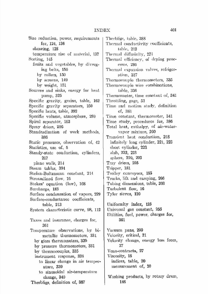
7/16/2019 Engenering Agriculture Perry
http://slidepdf.com/reader/full/engenering-agriculture-perry 421/422
INDEX 401
Size reduction, power, requirements
fol', 12'1, 136
~ h c [ \ r i n g , 128
tcmpcl'atUl'e l'iHC of mal erial, 137
Sorting, 145
fruits and vegetables, by eli ,'crg-
ing belts, HiO
by rollers, 150
by sere{ms, 149
by weight, 151
Sources and sinks, energy for ltr.fl t
pump, 325
Specific gravity, grains, table, ]62Specific gravity separators, 160
Specific heats, table, 3\)2
Specific volume, lltmosphel'e, 259
Spit'lll separator, 162
Spray driers, 296
Standardization of wo!'k methods,
386
Static prCSSll1'CS, observation of, 42
StlLtiStiCS, use of, 5
Stetldy-statc conduction, cylinders,217
plane walls, 21-1
Steam tables. 39,1
Stefan-Boltzmann constant, 2H
Streamlined flow, 16
Stokes' equation (law), 168
Surcharge, 183
Surface condensation of vapors, 229
SUl'faee-conductancc coefficients,
table, 213System ch:ln1cteristic curve, 98, 112
Tax('s and insurance, ebarges fol',
361Tmn]lGl'ature observat,ions, by bi-
metallie thermometers, 831
by glass thermometers, 329
by pressure thermometers, 331
by thermocouples, 335
instrument response, 338to linear change in air temper
ature, 339
to sinusoidal a i r ~ t e m p e r a t l l r echange, 340
Therbligs, definition of, 387
T I 1 ( ' l ' b l i g ~ , I able. il88
TIH'nnal conductivity ,'ocflicients,
l ahk 212ThplTllal diffmivity, 221
Thf'l'mal eHiciency, of drying proc
p ~ , ; e , ; . 286
Thennal ,'xpansion yalvp:,;, refriger
ation, 317
Thermocouple thermometers, 335
Thenuo('ouple wire combinations,
table, : ~ 3 { iThermometer, time constant of, 341
Throttling, ga,ge, 51Time ~ l l l d motion study, definition
of, 381
Time constant, thermometer, 3·11
Time study, prr)ce(\ures for, 386
Total heat, enthalpy, of llir-water-
vapor mixture, 2GO
Transirm t heat [l[mduetion, 218
infinitely loug eylinder, 221, 223
short e,y tillder, 223
Hlab, 222, 223sphere, 220, 223
Tray driers, 295
Tripper, 181
Trolley conveyors, 185
Trucks, lift [tnd carrying, 206
Tubing dimensions, tllble, 393
Turbulent flolV, 16
Tyler sieves, 120
Uniformity index, 123Universal gas constant" 255
Utilities, fllel, power, charges for,
361
V:tt:uum pans, 299
Velocity, critical, 21
Veloeity eh:mge, energy loss from,
27
Vena-contracta, 27
Viscosity, 18indices, table, 20
measurement of, 20
Washing products, by rott-uy drum,
146

7/16/2019 Engenering Agriculture Perry
http://slidepdf.com/reader/full/engenering-agriculture-perry 422/422
402 INDEX
Washing; products, by shuffle or
shaker washers, 148
by soaking, 146with brusheH, 148
with water sprays, 146
Water, cooling with i(:p., 228
Water sprayR, prorluct washing; with,
1<16
'Vater vapor pressure, in the at-
mosphere, 257
Weight sorters, 151Weights pel' gallon, fuels, table, 391Wet-bulb psychrometer, 342
Wet-bulb tomperature, 261
W81 ted perimeter, 18W urk economy prineiples, 381


![PDF] GEORGIA DEPARTMENT OF AGRICULTURE • GARY W. BLACK ...Lynyrd Skynyrd, The Band Perry will headline concert series at Georgia National Fair in Perry Classic Southern rock band](https://img.dokumen.tips/doc/110x75/612df92c1ecc515869428580/georgia-department-of-agriculture-a-gary-w-black-lynyrd-skynyrd-the-band.jpg)